Embed Size (px)
Citation preview

_______________________________________________________________
CREDIT Research Paper
No. 13/01______________________________________________________________
Determinants of Urban Worker Earnings in Ghana and
Tanzania: The Role of Education
by
Priscilla Twumasi Baffour
Abstract
The paper examines the role of education in earnings determination by usingall three rounds of the Urban Worker Surveys of Tanzania and Ghana for2004-2006. We investigate and compare heterogeneity in earningsdeterminants among self-employed (informal), private and public sectorworkers. We examine the role education, individual and householdcharacteristics play in facilitating entry into employment sectors in addition toanalysing the pattern of returns to education along the earnings distribution.After addressing endogeneity and selectivity biases associated with estimatingearnings equations, we find that education plays an important role inpromoting access to formal sector jobs, particularly employment in the publicsector, but has no direct impact on earnings within the sector in both countries.Results from quantile regressions indicate primary and secondary levels ofeducation are inequality-reducing among workers in Tanzania but this is notthe case in Ghana. Tertiary education on the other hand is found to widenearnings inequality in both Tanzania and Ghana.
JEL Classification:
Keywords: Education, Earnings, Employment Sector, Tanzania, Ghana_______________________________________________________________CREDIT, University of Nottingham

CREDIT Research Paper
No. 13/01
Determinants of Urban Worker Earnings in Ghana
and Tanzania: The Role of Education
by
Priscilla Twumasi Baffour
Outline
1. Introduction
2. Literature/ Model
3. Data / Specification
4. Results and Discussion
5. Concluding Comments
The Authors
The author is a Research Student in Development Economics in the School ofEconomics, University of Nottingham.
Contact e-mail: [email protected]
Acknowledgements
I am grateful to Professor Oliver Morrissey and Dr Trudy Owens for valuableguidance and comments.
_______________________________________________________________
Research Papers at www.nottingham.ac.uk/economics/credit/

1
1. Introduction
Human capital development (education) is fundamental to outcomes in modern
labour markets. This is evident in various studies in different countries and
time periods that undoubtedly confirm that better educated individuals earn
higher wages, experience less unemployment and work in more prestigious
occupations than their less educated counterparts. Psacharopoulos (1994)
showed the significant and robust positive relationship between education and
earnings is more or less universal (including middle and low income
countries). Other studies that endorse the positive returns to education
particularly at the primary level include Schultz (1999) and Psacharopoulos
(2002). These have been in part, the justification for the prominent feature of
policy in Sub-Saharan Africa (SSA) towards expanding primary education.
All these findings are based on the numerous theoretical explanations such as
Schultz (1961), Becker (1962; 1964) and Mincer (1974).
Recent empirical evidence on returns to education in Africa is mixed with
some bias towards convexity (see Soderbom and Teal 2003, Kingdon and
Soderbom 2007, Rankin et al 2010) which is a signal of skill shortage at high
educational levels and calls to question policy prescriptions in the region
tailored at primary education expansion. This therefore justifies the need for
more research into returns to education particularly at higher levels of
education.
Urban labour markets in developing countries are generally recognised as
having two distinct sectors, a regulated/protected formal sector and an
unregulated /unprotected informal sector (Pradhan and van Soest, 1995). Fields
(1995) introduced the notion of the ‘murky’ sector by extending Harris and
Todaro’s (1970) model of labour market segmentation by the concurrent
existence of an informal and a formal sector in urban labour markets. Here the
formal sector sets wages above market clearing levels that leaves a large pool
of unemployed. The informal sector therefore seems to absorb many job
seekers who are unable to secure employment in the stagnant formal sector of
employment. Recent empirical evidence on the other hand suggest the
possibility of viewing the informal sector as an efficient outcome of the labour

2
market that utilises technology intensive in unskilled labour that coexist with
the formal sector with comparatively skilled labour at much higher wages.
Maloney et al (2006) present evidence whereby small scale self-employment is
a preferred outcome and not due to inability of such individuals to find
rationed formal sector jobs.
In both Tanzania and Ghana, the self-employed outnumber wage employees by
almost twice in the urban labour market and it is the fastest growing segment
of the labour force across rural and urban areas, typical of most developing
nations particularly in Africa. Among the enormous challenges that face
governments in these countries as a result, is the need to identify development
strategies that can generate new employment and income opportunities to
reduce unemployment and under-employment. An understanding of the
earnings determination process in the informal sector is as a consequence vital
to understanding the labour market and income determination/distribution in
these countries.
Studies which analyse returns to education (determinants of earnings) typically
use the mincerian earnings model by relying on estimation methods such as
Ordinary Least Squares (OLS) or Instrumental Variables (IV); this estimates
the mean effect of schooling and other individual characteristic variables on
earnings. The standard methodology estimates how ‘on average’ schooling and
individual characteristics affect earnings; this yields straightforward
interpretations but may miss crucial information for policy purposes. Recent
empirical evidence by Bushnisky (1994, 1998), Mwabu and Schultz (1996),
Fitzenberger and Kurz (1998), Machado and Mata (2000), Nielsen and
Rosholm (2001), Kingdon and Soderbom (2007) indicate the level and change
in returns to education in the Mincerian model can differ across the earnings
distribution.
This paper consequently, aims to fill gaps in the earnings determination
literature on Africa by investigating and comparing heterogeneity in earnings
determinants across sectors (formal public and private sectors and the informal
(self-employment) sector) for Tanzania and Ghana with particular attention on
schooling. Firstly, we examine the role of education in the labour market in

3
terms of earnings by sector of occupation. Secondly, we examine the role of
education and individual and household characteristics in facilitating entry into
employment sectors (state) in a multinomial logit model of occupational
attainment and subsequently address selectivity bias in the earnings equation
following Heckman (1979) and Lee (1983). This is necessitated by the
important role education plays in labour market success by not only increasing
earnings but by the indirect promotion of entry into well paid occupations. We
further apply quantile regression to look at earnings determinants across
quantiles of the conditional earnings distribution. This enables us to examine
whether returns (premiums) to education and other earnings determinants for
urban workers in both countries are identical for low and high earners and shed
light on whether education ameliorates or worsens existing inequalities.
We utilise the Urban Household Worker Survey (UHWS) on Tanzania and
Ghana. This data is suitable for this study because it provides information on
imputed earnings figures for the self-employed (informal sector) in addition to
the regulated formal sectors (public and private). This allows for comparison
across occupations and shed more light on the importance of heterogeneity in
earnings determination. The study uses all three rounds of the UHWS of 2004,
2005 and 2006 in pooled sample estimations with year dummies to capture all
effects that are common at a particular point in time.
The following section presents our theoretical framework and empirical
literature; this is followed by the methodology in section 3. Section 4 is on the
data and empirical strategy for estimating earning determinants with emphasis
on the role of education. Here we adopt two specifications of the earnings
equation; one is a standard linear model with years of education and a second
model with dummy variables for levels of education. Additional attempt is
made to address the endogeneity bias by using instruments; sample selection
bias due to estimation for sub samples is also addressed. Finally, earnings
functions are estimated by quantile regressions to identify heterogeneities in
earnings along the earnings distribution. Results are presented in section 5 and
the final section concludes.
4
2. Literature/ Model
The estimation of the profitability of investment in education is arrived at
using two different methods, the ‘full’ or ‘elaborate’ method and the ‘earnings
function’ method, these in theory give very similar results. The method
adopted in most studies is dictated by the nature of data available. The
elaborate method uses detailed age-earnings profiles by level of education to
find a discount rate that equates a stream of education benefits to a stream of
education cost at a given point in time. The basic earnings function method is
due to Mincer (1974) and involves the fitting of a semi-log ordinary least
squares regression using the natural logarithm of earnings as the dependent
variable and years of schooling and potential labour market experience and its
square as independent variables. In this semi-log earnings function
specification, the coefficient on years of schooling can be interpreted as the
average private rate of return to an additional year of education, regardless of
the educational level to which this year of schooling refers. The extended
earnings function method is also used to estimate returns to education at
different levels by converting the continuous years of schooling variable into a
series of dummy variables that refer to the completion of the main schooling
cycles (primary, secondary and tertiary education, or drop out of these levels or
even different levels of curriculum (vocational versus general) within an
educational level. The private rate of return to the different levels of education
is consequently derived by comparing adjacent dummy variable coefficients.
Analysis of the demand for education has been driven by the concept of the
human capital pioneered by Schultz (1961), Becker (1964) and Mincer (1974).
Education in human capital theory is seen as an investment of current
resources (the opportunity cost of the time involved as well as any direct costs)
in exchange for future returns (expected higher earnings). The standard model
for the development of empirical estimation of returns to education is based on
the relationship derived by Mincer. The typical human capital theory (Becker,
1964) assumes level of education is chosen to maximise expected present
value of the stream of future incomes net of the costs of education. The basic
assumption in this model is that an individual’s earnings reflects labour
productivity and that investment in human capital in the form of foregone

5
earnings in the past pays off in higher wages in the future Card (1999). With
this, Mincer developed a theoretical model from wage (earnings) equation. The
Mincerian earning function has been used predominantly in many studies due
to the increased availability of micro data. In the original study Mincer (1974)
used 1960 US Census data and used an experience measure known as potential
experience (i.e. current age minus age left full time schooling) and found that
the returns to schooling were 10% with returns to experience of around 8%.
Layard and Psacharopolous (1979) similarly found returns to schooling to be
around 10% in Great Britain.
In the empirical application, the schooling measure is treated as exogenous,
although education is an endogenous choice variable in the underlying human
capital theory. In addition, the Mincer specification of the disturbance term
captures unobserved individual effects such as ability or motivation which also
influence the schooling decision and induce a correlation between schooling
and the error term in the earnings function. If schooling is endogenous then
estimation by least squares methods will yield biased estimates of the return to
schooling.
A number of approaches have been proposed in the literature to deal with
endogeneity problem. First of all, measures of ability have been incorporated
to proxy for unobserved ability. Such studies include IQ and related tests as
proxies (Grilches 1977, Griliches and Mason 1972). This is expected to reduce
the estimated education coefficient if it acts as a proxy for ability, so that the
coefficient on education captures the effect of education alone given that,
ability is controlled for. Results of such studies suggest an upward bias in
results that lack an ability measure. The method of adding ability proxies has
however been criticised in literature because, it is very difficult to develop
ability measures that are not determined by schooling. The second approach
exploits a belief that siblings are more alike than a randomly selected pair of
individuals, since they share common heredity, financial support, geographical
influences and peer influence. The idea behind this strategy is that some of the
unobserved differences that bias a cross-sectional comparison of education and
6
earnings are reduced or eliminated within families.1 This approach attempts to
eliminate omitted variable bias by estimating the return to schooling from
differences between siblings or twins in levels of schooling and earnings. It
uses with-in twins or with-in sibling’s differences in wages and education by
accepting the assumption that unobserved effects are additive and common
within twins. Given that siblings have the same level of ability (the omitted
variable), any estimate of schooling from within family data is expected to
eliminate this bias. This is a modification of a more general fixed effect
framework in individual panel data, where unobserved individual effect is
considered time-invariant. This approach however, has been criticised on two
grounds. First, if ability has an individual component in addition to the family
component, which is not independent of schooling variable, then the within-
family approach may not yield estimates that are less biased than OLS
estimates. Secondly, if schooling is measured with error, it will lead to a larger
fraction of the differences between twins than across the population as a whole
(Ashenfelter et al, 1999). Conclusions from within-twin studies suggest ability
bias is relatively small when measurement error has been controlled for.
The final approach to deal with ability bias, exploits the natural variation in
data caused by different influences in the schooling decision. The core of this
natural experiment approach is to provide a suitable determinant (instrument)
for schooling that is not correlated with the earnings residual. The treatment
group is chosen (though not randomly) independently of individual
characteristics. The treatment and the control groups should be identical in
both observed and unobserved characteristics that affect earnings except for
schooling. The construction of instruments that are uncorrelated with the
earnings residual means instrumental variable (IV) approach will generate a
consistent estimator of the return to schooling. The (IV) estimator proceeds in
two stages; the effect of the instrumental variable on schooling is estimated
first, and then the effect of the instrumental variable on earnings is estimated.
By assumption, given that the instrument is correlated with earnings only
because it influences schooling, the ratio of the effect of the instrument on
1 Within family estimator can be given an IV interpretation; the instrument for schooling is the deviation
of an individual’s schooling from the average for his or her family.

7
earnings to its effect on schooling provides an estimate of the causal effect of
schooling on earnings. The main criticism of IV estimates is the concern that
the instrument may not actually be truly independent of the earnings residual.
IV studies however, differ in terms of results, a number of them indicate the
presence of a downward bias in OLS estimates. Card (1998) proposed an
explanation for this phenomenon that is based on the hypothesis of
heterogeneous returns to schooling that declines at higher levels of schooling.
IV estimates differ from OLS estimates by the extent to which the instrument
influences schooling decisions at different levels. If the instrument influences
decisions primarily at lower levels of schooling, the IV estimator may be
higher than OLS estimator because it reflects the payoff to schooling at lower
rather than higher schooling levels.
In instrumental variables estimation, the probability limit of the IV estimator is
unaffected by measurement error in schooling2. This has the tendency for an
IV estimator to exceed the corresponding OLS estimator of the effect of
schooling on earnings. In addition, the validity of a given IV estimator
critically depends on the assumption that the instruments are uncorrelated with
other latent characteristics of individuals that may affect their earnings.
While recent research on schooling use institutional features of the educational
system to identify causal effect of schooling, family background information
such as mother's and father' s education have been used in most studies either
directly to control for unobserved ability or as instrumental variables for
completed education. The curiosity in family background is driven by the fact
that children's schooling outcomes are very highly correlated with the
characteristics of their parents, particularly with parents' education.
In spite of the strong intergenerational correlation in education, family
background measures as instruments for completed education have been
questioned, even if family background has no independent causal effect on
earnings. However, due to data availability issues especially in Africa, family
background measures continue to be used and considered to be legitimate
instruments. Instrumental variables have been widely used in empirical work
2 Assumes the instrumental variable is uncorrelated with the measurement error in schooling
8
on schooling as a standard solution to the problem of causal inference. The
landmark study by Angrist and Krueger (1991), employed a ‘natural
experiment’ instrument strategy by assuming quarter of birth (interacted with
year or state of birth in some specifications) is uncorrelated with earnings
except through its effect on education through school-start age policy and
compulsory school attainment laws. The study concluded subsequently that,
men born from 1930 to 1959 with birth dates earlier in the year have slightly
less schooling than men born later in the year. This was attributed to
compulsory schooling laws where people born in the same calendar year
typically start school at the same time. As such, individuals born earlier in the
year reach the minimum school-leaving age at a lower grade than those born
later in the year. This allows individuals who want to drop out as soon as it is
legally possible, to leave school with less education. They found IV estimates
of the return to education are on average higher than the corresponding OLS
though the difference between the IV and OLS estimators were statistically
insignificant. Their findings of little differences between OLS and IV estimates
for the United States, suggested schooling endogeneity is not empirically an
important source of parameter bias.
The findings of Angrist and Krueger have attracted a lot of interest and
criticism in literature. Bound et al. (1995) indicate a problem of weak
instruments in some of the specifications in Angrist and Krueger's IV models.
Bound and Jaeger (1996), also criticised Angrist and Krueger's findings with
the proposition that quarter of birth may be correlated with unobserved ability
differences. Bound and Jaeger examined the schooling outcomes of earlier
cohorts of men who were not subject to compulsory schooling institutions and
found some evidence of seasonal patterns. They additionally discussed
evidence from the socio-biology and psychobiology literature which suggests
that season of birth is related to family background and the incidence of mental
illness. This called to question, the explanatory power of the instruments used
9
by Angrist and Krueger.3 Staiger and Stock (1997), used a limited information
maximum likelihood (LIML) approach with quarter of birth interacted with
state of birth and year of birth as instruments to examined the same data used
by Angrist and Krueger (the 1980 Census). They confirmed high IV estimates
above corresponding OLS estimates can make one infer that asymptotically
unbiased estimates of the causal effect of education are even higher.
Card (1999) compared the mean levels of parents' education by quarter of birth
for children under one (1) year of age in a 1940 census in the United States.
The comparison of the mean years of education for mothers and fathers of
children born in each quarter by Card, led to the conclusion that, there is no
indication children born in the first quarter come from relatively disadvantaged
family backgrounds. This suggested the seasonality patterns identified by
Angrist and Krueger are probably not caused by differences in family
background.
A study by Kane and Rouse (1993) about the relative labour market valuation
of credits from regular (4-year) and junior (2-year) colleges made findings that
suggest credits awarded by the two types of colleges are interchangeable.
Consequently, they measure schooling in terms of total college credit
equivalents. Kane and Rouse compared OLS specifications against IV models
that used distance to the nearest 2-year and 4-year colleges and state-specific
tuition rates as instruments in the analysis of earnings effects of college credits.
Their IV estimates were 15-50% above the corresponding OLS specifications.
Card (1995b), examined schooling and earnings differentials associated with
growing up near a college/university and found when college proximity is used
as an instrument for schooling in the Young Men sample of a U.S. National
Longitudinal Survey (NLS), the IV estimator subsequently, is considerably
above the corresponding OLS estimator, though not very precise. This is
consistent with the idea that accessibility matters more for individuals on the
margin of continuing their education. College proximity is found in the study
3 Angrist and Krueger (1992) used the Vietnam-era draft lottery in conjunction with educational
deferments to provide instruments for education in another natural experiment. They again find only
a slight upward bias in the ordinary least squares estimated returns after showing that the
instruments have strong explanatory power.

10
to have a bigger effect for children of less-educated parents and hence suggests
an alternative specification that uses interactions of college proximity with
family background variables as instruments for schooling, and includes college
proximity as a direct control variable. The IV estimate from this interacted
specification is to some extent lower than the estimate using college proximity
alone, but about 30% above the OLS estimate.
Maluccio (1997) applied the school proximity idea on rural Philippines. The
study combined education and earnings information for a sample of young
adults with data for their parents' households which included the distance to
the nearest high school and an indicator for the presence of a local private high
school. The variables show a relatively strong effect on completed education in
the sample and the OLS estimates and conventional IV models that used
school proximity as an instrument, in addition to IV models that include a
selectivity correction for employment status and location. Results from both IV
estimates are considerably above corresponding OLS estimates. Other studies
that have found high IV estimates over OLS include Conneely and Uusitalo
(1997) and Ichino and Winter-Ebmer (1998).
The findings that emerge from the above studies on OLS and IV estimators
lead to the conclusion that instrumental variables estimates of the return to
schooling characteristically exceed the corresponding OLS estimates. With the
assumption on a priori grounds that OLS methods lead to upward-biased
estimates of the true return to education, then, larger IV estimates obtained in
many current studies leads to a dilemma. Bound and Jaeger (1996), Griliches
(1977) and Ashenfelter and Harmon (1998) have all offered hypothesis to
explain this dilemma.
The above studies reviewed and others suggest the returns to education are
biased downward in an ordinary least squares regression, even though it is
unclear how to account for the results. In the case of developing countries, the
evidence is mixed, mostly due to incomparability of results across studies.
Behrman (1990) reviewed existing studies and concluded by citing several
studies that, most standard estimates overstate the return to education. Few of
the studies however simultaneously controlled for endogeneity and

11
measurement error and others used earnings rather than wage data. Strauss
and Thomas (1995) reviewed additional studies and suggests the evidence is
inconclusive and warrant further studies. The study further proposed the use of
an expanded set of instruments that include indicators of the availability of
schooling and household resources measured contemporaneously with an
individual’s schooling decisions.
In Africa, numerous studies on schooling and earnings have used different
methods and instruments to address problems of endogeneity. In a recent study
on Tanzania by Soderbom et al. (2006), repeated cross-section surveys on
Tanzanian and Kenyan manufacturing sectors were used in a control function
approach to correct for endogenous education by instruments. Results
generally, showed a pattern of upward biased OLS estimates contrary to the
more recent studies reviewed for mainly developed countries. Subsequently,
the conclusion from the study was contrary to the conventional view of
concavity between earnings and education. The marginal return to education
was found to increase with increased education in both Tanzania and Kenya,
an indication of a convex earnings function with education.
In a study by Rankin, Sandefur and Teal (2010), the 2004 and 2005 rounds of
the Tanzania and Ghana Household Worker survey were used in a pooled
estimation to investigate the role of formal education and time spent in the
labour market to explain labour market outcomes of urban workers in Ghana
and Tanzania. The study adopted the standard Mincerian earnings function and
controlled for endogenous education by education supply side variables in
addition to family background in four models (self employment, public sector,
small and large). After controlling for selection bias the paper concludes, the
existence of a convex returns to education in self employment though average
returns are low in this sector and a concave returns to education in large firms,
this does not depend on how selection is modelled but depends on selection. In
the public sector however, no returns to education is found in both countries.
A study by Quinn and Teal (2008), used three rounds (2004, 2005 and 2006) of
the Tanzanian Household Worker survey in a panel study to examine
determinants of earnings and earnings growth from 2004-2006. The study

12
pooled all three rounds of the data in an OLS estimation of earnings equation.
Results indicate a significant convex effect of education on earnings, with
substantial heterogeneity between and within sectors. These results are shown
to be robust to control of endogenous education with instruments.
Soderbom et al. (2007), in a study on education, skills and labour market
outcomes in Ghana, used the Ghana Living Standards survey for 1998-99 in a
three sector model of wage employment, self-employed and agricultural
workers. Labour market returns to literacy and numeracy skills in addition to
analysing the pattern of returns to education along the earnings distribution
was examined. The study used household fixed effects earnings function to
address endogeneity of schooling among wage workers and finds the fixed
effects returns to education for men increases but that for women decreases
though none of their estimates was statistically different from their OLS
estimates. The study further corrected for sample selectivity bias by using
Heckman (1979) and Lee (1983) selection correction method and concluded
that, education raises earnings by indirectly helping individuals to gain entry
into high paying occupations (wage employment) but has low direct effects on
earnings. In addition, they found education to be inequality-reducing in wage
employment in Ghana.
In Kenya, Wambugu (2002) used a survey of rural households 1994 to model
employment sector choice in a five way multinomial logit model of
agricultural sector, public sector, private sector, informal sector and unpaid
family workers. The study found high levels of education to increase
probability of participation in formal sector employment, specifically; men
with more than primary education have low probability of entry into the
informal sector whiles those with less than full secondary education have
reduced chances of agricultural employment. Women in households with lands
were found to be less likely to work off the farm. The study concluded that the
highest returns to primary education is in the informal sector while that of
secondary education is highest in the private sector and that correcting for
sample selection bias does not to alter estimates except for women in the
public sector.

13
Studies that have utilised quantile regression method within the Mincerian
framework include Buchinsky (1994), who proves the returns to education in
the U.S increase considerably over the quantiles of the conditional distribution
of wages. Fitzenberger and Kurz (1998), Machado and Mata (2000), all found
varying returns across quantiles of the wage distribution. Mwabu and Schultz
(1996), in a similar manner used quantile regression on a sample of South
African men and obtained varying returns across quantiles. Nielsen and
Rosholm (2001), Kingdon and Soderbom (2007) all applied quantile method
and obtained similar results that confirm heterogeneity in returns to education
along the conditional wage distribution and the justification for quantile
regression technique in returns to education studies. We as a result find it
necessary to adopt this methodology in addition to using the standard
methodologies and addressing the issues of endogeneity in returns to education
estimates in a comparative study on existing data on Tanzania and Ghana.
Methodology
In this section, we discuss the estimation technique used and some of the
econometric issues encountered. We adopt Mincer (1974) model based on the
fundamental assumption that an individual’s earnings reflect his labour
productivity and that investment in human capital in the form of foregone
earnings in the past pays off in higher wages in the future (Card 1999). This
led to the development a theoretical model from which the following wage
equation is derived
2
0 1 i 2 i 3 i i ............................ 1log S ui iw X x x
Where wi is an earnings measure for individual i such as earnings per hour,
week or month. Si represents a measure of schooling, this proxy’s human
capital acquired through formal education, xi is an experience measure
(typically age – the age an individual left school), this captures human capital
acquired on-the-job. Xi is a set of other variables assumed to affect earnings
and ui is the disturbance term which captures all factors other than schooling
and labour market experience that affect wages. The derivation of the

14
empirical model by Mincer implies, under the assumptions made (particularly
of no tuition cost). β1 can be considered the private financial return to
schooling as well as the proportionate effect on wages of an increment in S.
In this study, OLS is used to estimate earnings equations as a baseline in the
following model
+=∝ݓ ߚ + ݑ (2.1)
Here, wi is the monthly earnings of individual i, Xi is a vector of worker
characteristics (list of explanatory variables) and ui is the residual. According
to Card (1999), the choice of time over which to measure earnings is mostly
dictated by data availability. The explanatory variables include the log of hours
of work, education (highest educational level completed), tenure (the duration
on the job as a proxy for experience) and gender dummy to control for
disparities in earnings by sex as well as occupational and firm level variables.
Labour market tenure is included in linear and quadratic form to identify the
shape of tenure earnings relationship. The estimated parameters ,መߚ are
computed by minimising the sample’s sum of squared residuals;
=�ොଶݑ ൫ − �′ߚመ൯ଶ
(2.2)
OLS estimators are the best linear unbiased estimators as suggested by the
Gauss-Markov theorem with minimum variance in the class of all linear
unbiased estimators, on condition that the OLS estimates comply with the
assumptions of the classical linear regression. Violation of any of the
assumptions makes OLS estimates inefficient, possibly biased and inconsistent
(Greene, 2003). The presence of heteroskedasticity violates the assumption of
the classical linear regression of constant conditional variance; this does not
produce biased estimates but incorrect standard errors. We subsequently use
robust standard errors.
Beneath the assumption of no other cost of education rather than foregone
earnings, the estimated coefficient of the education (schooling) variable
directly measures the returns to one additional year of education in terms of
(log) earnings.

15
The use of years of schooling implicitly suggests that one additional year of
schooling, regardless of the current level of education, yields the same return.
This may not be the case if, for example, completed degrees rather than years
of schooling itself are valued in the labour market. As a result, in addition to
the quantitative specification, we allow education to affect earnings in a non-
linear way by the inclusion of dummy variables for the highest completed
educational level in the earnings function. Corresponding coefficients in this
regard, represent the wage premium associated with the different education
levels compared to the reference group (no education). Empirical analysis is
carried out based on three labour market sub-sectors which are public sector,
private sector, self-employment in addition to a pooled model.
Endogeneity bias
Two main sources of bias in OLS estimates of effects of education on earnings
are endogeneity (omitted variable) bias and sample selectivity bias. The former
relates to the concern in earnings literature that education may be positively
correlated with unobserved ability which will lead to an upward bias of
estimates of the returns to education.4 Therefore, to be sure our findings are not
due to the failure to allow for such endogeneity. Instrumental variables are
used to control for endogenous education.
Endogeneity is caused by a correlation between explanatory variables and the
disturbance term. This means;
(ݑ,ݔ)ݒܥ ≠ 0 (2.3)
This results in biased and inconsistent estimates; which is corrected by an
identification of variable(s) that are not correlated with the residual but
correlated with the endogenous variable. If we denote the instrumental
variables as z, the following condition must hold:
4 Belzil and Hansen (2002) find a strong and positive correlation between unobserved ability and
unobserved taste for schooling which leads to a substantial upward bias of OLS estimates of returns to
schooling. However, recent findings in empirical literature indicate that estimated returns rise as a result
of treating education as an endogenous variable, Card (2001).

16
(ݑ,ݖ)ݒܥ = (ݖ,ݔ)ݒܥ�0� ≠ 0 (2.4)
A good instrument is highly correlated with the endogenous variable and
uncorrelated with the residual. If condition 2.4 is satisfied, a two-stage least
squares (2SLS) can produce consistent estimates.
If we assume in a reduced form, schooling is given by
ݏ = .ߙ ݖ + �ߜ (2.5)
Where zi is a vector of instruments independent of δi but uncorrelated with ui in
the structural equation. This requires valid exclusion restrictions (variables
correlated with schooling but uncorrelated with the earnings residual). As a
result, we use family background variables, specifically father and mother’s
education as instruments for education.
Sample Selection bias
OLS estimates are the best linear unbiased estimates if they comply with the
assumptions of the classical linear regression. In this study, there is the
possibility of violation of some of the assumptions for which reason, the
disturbances are no longer normally distributed as expected as .(ଶߪ,0)~ߤ
This suspicion is because in developing countries (Africa), having a job in the
formal wage sector is typical of outcomes in the labour market (selection into
different sectors of employment are correlated with the potential determinants
of earnings). In addition, observations with no earnings information are
excluded, if exclusion of such observations is not random (lower earners are
less likely to work), such sample selection bias may bias OLS estimates.
Estimation of equations over an endogenously selected population requires the
implementation of selection correction methods following Heckman (1979).
When selection is presumed to be over a large number of exclusive choices,
the multinomial logit specification is applied Lee (1983) and Durbin and
McFadden (1984).
We therefore model occupational outcomes by focusing on the way in which
education and other individual and household characteristics influence
people’s decisions to participate in the formal public or private sectors and
17
self-employment relative to unemployment for consistent estimates of the
earning function.
Labour force Participation Model
Participation decision in the labour market is assumed to be a function of
variables that influence a person’s expected offer wage and reservation wage.
An individual chooses to enter the labour market if the offer wage is greater
than the reservation wage. Human capital variables are expected to influence
the offer wage while household characteristics may influence the reservation
wage by affecting productivity in the home and demand for leisure.
The multinomial logit model adopted, assumes each individual selects among
four mutually exclusive alternatives in the labour market: working in the
public sector (indexed pu), working in the private sector (indexed pr), self-
employment in the informal sector (indexed s) and unemployment (indexed u).
An individual compares the maximum utility attainable given each
participation alternative and selects the alternative which yields the maximum
utility.5 Preferences are described by a well-behave utility function whose
arguments include the household time of the individual, a Hicksian composite
commodity and a vector of exogenous constraints on current decision making.
Preferences are maximised subject to time and income constraints with no
uncertainty.
If Vji is the maximum utility attainable for individual i if he/she chooses
participation status j=pu, pr, s, u and suppose this indirect utility function can
be decomposed into a non-stochastic component (S) and a stochastic
component (є):
V�= S�+ є�����������������������������������������������������������������������������������������������(3.1)
5 The specification does not allow the possibility of working concurrently in more than one sector. This
restriction may be unreasonable if individuals work both in a family business and in the formal sector.
However, the data does not have information on multiple job holding. Each person reports one current
employment status.

18
where Sji is a function of observed variables and єji is a function of unobserved
variables. The probability that individual i will select the jth participation status
is given by
Pji = Pr[Vji > � ki ] for k ≠ j, k = ,[ݑ,ݏ,ݎ,ݑ� (3.2)
or, substituting in from (1),
Pji = Pr[Sji – Ski > єk �− є��for k ≠ j, k = [ݑ,ݏ,ݎ,ݑ� (3.3)
If the stochastic components have independent and identical Weibell
distributions, the the difference between the errors (єki - єji) has a logistic
distribution and the choice model is multinomial logit (McFadden, 1974).6
This is a direct extension of a binary logit model to a dependent variable with
several unordered categories since the decision to work in a particular sector is
not sequential or ordered; rather this depends on the sector in which an
individual finds a job.7
In order to estimate this model, a functional form of the non-stochastic
component of the indirect utility function Sji must be specified. When
approximated in a linear form (Sji = βjXi), yielding an empirical specification
of the form
=൯ߚ൫ݔ
+௨൯′ߚ൫ݔ +൯′ߚ൫ݔ exp൫ߚᇱ௦൯+ (௨′ߚ)ݔ
(3.4)
where Xi is a vector of independent variables that explain labour force
participation and βj is the parameter vector.
Coefficients obtained in the logistic estimation serve to provide a sense of the
direction of the effects of the covariates on participation and sector choice in
the labour market but cannot be used for magnitude of impact analysis. To
examine the magnitude of impact, we calculate the average partial effects of
6 Weibull distribution has a unimodal bell shape roughly similar to the normal distribution.
7 Some individuals decide to join the informal sector while awaiting modern wage employment job,
others also leave modern sector jobs to become self-employed in the informal sector and vice versa. The
choices made, do not follow any particular order and this serves as a justification for the MNL model.

19
the covariates on the probability of participation in the different labour market
state.
The criticism of the multinomial logit model is the independence of irrelevant
alternatives (IIA). Bourguignon, Fournier and Gurgand, 2007 in Monte Carlo
experiments, show that the selection bias correction based on the multinomial
logit model can provide fairly good correction for the outcome equation even
when IIA assumption is violated.
Following Heckman (1979) and Lee (1983), the earnings equation can be
corrected for selectivity by including the inverse of Mills ratio8 (selection
correction term) as an additional explanatory variable in the earnings equation.
+=∝ݓ ߚ + +ߣߩ (ଶߪ,0)~ݑ�;ݑ (4.1)
where ݓ is the is monthly earnings of individual i in sector j, Xij represent
explanatory variables, βij are estimated parameters, ߣ is the selectivity
correction term and ߩ measures the effect and direction of non-random
selection into employment sectors, if this is statistically significant, the null
hypothesis of ‘no bias’ is rejected.
Quantile Regression
It is possible that earnings determinants, particularly education may be
different for individuals at different points in the earnings distribution.
Standard OLS techniques concentrate on estimating the mean of the dependent
variable subject to values of the independent variables where variables are
included as uncentred regressors. As an alternative to OLS, quantile regression
is based on the entire sample available and allows us to estimate the return to
education within different quantiles of the earnings distribution (Buchinsky,
1994). In particular, while OLS captures the effect of education and other
covariates of an individual on the mean earnings, quantile regression look at
the determinants at some other points of the earnings distribution for example
8 The inverse Mill’s ratio is defined as =ߣ∅(ுೕ)
ః (ுೕ), where ܪ = )ଵߔ ), ∅(. )
is the standard normal
density function, Φ(.) the normal distribution function, and is the estimated probability that the ith
worker chooses the jth occupation.

20
bottom or top quartile. In essence, we focus on quantile treatment effects of
education and other covariates on earnings rather than on the average treatment
effect and this add value to estimation results.
The estimation of the model at different quantiles enables us to trace the entire
conditional distribution of earnings given a set of regressors. Afterwards,
comparing the estimated returns (premiums) across the whole earnings
distribution, we can infer the extent to which education exacerbates or reduces
underlying inequalities. Particularly, how schooling, individual characteristic,
sector of employment and firm size affect earnings differently at different
points of the conditional distribution of earnings. An additional advantage of
employing this estimation method is that the regression coefficient vector is
not sensitive to outlying values of the dependent variable, as the quantile
regression objective function is a weighted sum of absolute deviations.
Provided error terms are homoscedastic, according to Koenker and Bassett
(1982) and Rogers (1992), this method would be adequate to calculate the
variance –covariance matrix. Rogers (1992), shows in the presence of
heteroscedastic errors, this method understates the standard errors. We
consequently use bootstrapped estimator of standard errors as suggested by
Roger to cater for any such under estimated standard errors. This method
however requires that, there is adequate dispersion of the independent
variables over the earnings distribution to enable identification of coefficients
for each quartile. The Tanzania and Ghana urban household worker surveys
appear satisfactory in this regard.
According to Koenker and Bassett (1978), quantile regression estimation is by
minimising the following equation;
minఉఢோೖ ∑ −௧ݕ|ߠ |ߚ௧ݔ +௧ఢ(௧:௬ஹ௫ఉ) ∑ (1 − −௧ݕ|(ߠ ௧∈(௧:௬�ழ௫ఉ)|ߚ௧ݔ (5.0)
Where yt is the dependent variable, xt is the k by 1 vector of explanatory
variables, β is the coefficient vector and 1 is the quantile to be estimated.
Following Bushnisky (1994, 1998), the quantile regression model of the
earnings function can be specified as follows;
lnݓ�= +ߚ′ݔ �������������������������������������������������������������������ఏݑ (5.1)
21
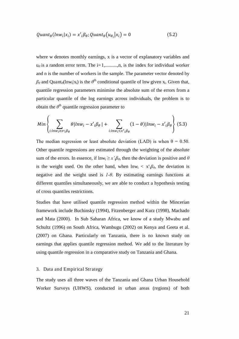
)ఏݐݑ (ݔ|ݓ = =൯ݔఏหݑఏ൫ݐݑ;ఏߚ′ݔ 0 (5.2)
where w denotes monthly earnings, x is a vector of explanatory variables and
uθ is a random error term. The i=1,..........,n, is the index for individual worker
and n is the number of workers in the sample. The parameter vector denoted by
βθ and Quantθ(lnwi|xi) is the θth conditional quantile of lnw given xi. Given that,
quantile regression parameters minimise the absolute sum of the errors from a
particular quantile of the log earnings across individuals, the problem is to
obtain the θth quantile regression parameter to
ܯ ቐ |ߠ −ݓ ఏߚ′ݔ:௪ஹ௫ᇱఉഇ
| + (1 − |(ߠ ݓ
:௪ழ௫ᇲఉഇ
− ఏቑ�(5.3)ߚ′ݔ
The median regression or least absolute deviation (LAD) is when θ = 0.50.
Other quantile regressions are estimated through the weighting of the absolute
sum of the errors. In essence, if lnwi ≥ x’iβθ, then the deviation is positive and θ
is the weight used. On the other hand, when lnwi < x’iβθ, the deviation is
negative and the weight used is 1-θ. By estimating earnings functions at
different quantiles simultaneously, we are able to conduct a hypothesis testing
of cross quantiles restrictions.
Studies that have utilised quantile regression method within the Mincerian
framework include Buchinsky (1994), Fitzenberger and Kurz (1998), Machado
and Mata (2000). In Sub Saharan Africa, we know of a study Mwabu and
Schultz (1996) on South Africa, Wambugu (2002) on Kenya and Geeta et al.
(2007) on Ghana. Particularly on Tanzania, there is no known study on
earnings that applies quantile regression method. We add to the literature by
using quantile regression in a comparative study on Tanzania and Ghana.
3. Data and Empirical Strategy
The study uses all three waves of the Tanzania and Ghana Urban Household
Worker Surveys (UHWS), conducted in urban areas (regions) of both

22
countries9. The samples are based on a stratified random sample of urban
households from the 2000/01 Household Budget Survey (HBS) for Tanzania
whiles that of Ghana is from the 2000 census in Ghana. The surveys have been
conducted in 2004, 2005 and 2006. Survey questions include: levels of
education and other training and qualifications in addition to individual and
household characteristics. Information on jobs include: type and length of each
episode of employment; remuneration; and other sources of income. The unit
of analysis in the data is the individual. The UHWS data has a feature which is
important in answering the questions posed in this paper, as it provides
comparable information including income data on both formal and informal
(self-employment) sector workers. The study uses all three waves of the data
for the respective countries in pooled samples with year dummies to control for
time trend.
The three rounds of the UHWS for Tanzania and Ghana after cleaning consist
of the following for the respective years: 2004 (1818 in Ghana and 653 in
Tanzania), 2005 (895 in Ghana and 443 in Tanzania) and 2006 (309 in Ghana
and 572 in Tanzania). There is a small panel dimension and recall aspect of
the data that is not used in this study.
The sample for Tanzania is summarised in tables 1, 2 and 3 in terms of
employment status by gender, years of education and tenure on the job,
average earnings by employment sector, gender and level of education. As
shown in table 1, individuals active in the labour market are categorised into
formal public sector employment, formal private sector employment, informal
sector (self-employment) and not-working (this includes unpaid family
workers and the unemployed). Overall, the informal sector (self-employment)
category is the largest sector in terms of employment (42.4%), followed by
not-working (33.9%), private (16.5%) and public (7.3%) respectively.
Average years of schooling and tenure on the job for public sector workers are
more than all other sectors. Individuals not-working for income are the least
educated in the sample followed by the self-employed with the private sector
worker being more educated than the self-employed. This suggest the
9 Surveys are conducted by the Centre for the Study of African Economies at the University of Oxford.

23
existence of a hierarchy in occupations in terms of education with public sector
employment at the top consisting of the most well paid and better educated,
private sector as the next and self-employment as the last. Average years of
tenure on the job are higher in self-employment than in private sector.
Generally, the long years of tenure on average depicted in the table across all
sectors may suggest labour turnover is low in the Tanzania labour market.
Important differences also emerge between males and females when we
decompose employment status by gender. Though females constitute 54%
(percent) of the sample, their proportion is less than males in all employment
types, as 41% of females are not-working compared to 25.6% males.
Average monthly earnings by employment sector and gender presented in table
2 shows huge differences in earnings between public sector employed people
and those in either private or self-employment. Average earnings in public
sector are about 133% and 264% more than private sector and self-
employment earnings respectively. However, since earnings distribution is
mostly skewed, the mean can be a misleading measure of central tendency, but
figure 1 shows the distribution of the log of earnings and confirms the
hierarchy in earnings between sectors. Disaggregation of earnings by gender
shows men on average earn more in all sectors than women. A further
disaggregation of earnings by level of education (table 3) indicates incremental
returns by level of education since average earnings to individuals with high
levels of education are more than those with low or no education (table 3).
52% of individuals in the sample have primary education followed by
secondary education of 31%, 13% with no education and 3% with tertiary
education.

24
Table 1: Labour Market Status Distribution by Gender with Education andTenure for Tanzania
Employment Status All (%) Female (%) Male (%) Education(yrs)
Tenure(yrs)
Public 7.30 7.19 7.39 11.91 17.44
Private 16.45 10.84 23.23 8.25 8.91
Self- employment 42.39 40.98 43.74 7.27 10.77
Unemployment 33.86 40.98 25.64 6.33 -
Total 1,465 793 663 7.40 11.04
Source: Calculations from Tanzania UHWS 2004, 2005 and 2006
Table 2: Average Monthly Earnings by Employment Sector and Gender;Tanzania
Employment Sector All ($) Female ($) Male ($)
Mean Std. dev Mean Std. dev Mean Std. dev
Public 134.66 137.96 131.56 146.49 140.54 129.38
Private 57.71 60.69 48.36 46.73 62.95 66.99
Self-employment 36.89 65.56 27.72 33.47 46.99 87.40
Total 52.90 81.63 44.14 69.77 61.33 90.91Source: Calculations from Tanzania UHWS 2004, 2005 and 2006
Table 3: Monthly Earnings by Employment Sector and Educational level;Tanzania
All Public Private Self-employment
Mean Std.dev Mean Std. dev Mean Std. dev Mean Std.dev
No Education 25.08 35.39 64.49 53.47 28.42 31.01 22.46 34.80
Primary 34.92 42.92 69.28 35.40 38.56 33.87 31.66 45.30
Secondary 71.92 82.63 134.24 97.11 81.75 66.89 45.92 70.73
Tertiary 162.76 213.36 208.45 243.54 119.07 114.11 142.71 253.21
Source: Calculations from Tanzania UHWS 2004, 2005 and 2006

25
Figure1: Sample Distribution of Earnings by Sector: Tanzania
Comparable summary of the Ghana sample are provided in tables 4, 5 and 6.
The sample distribution by sector and gender in table 4 shows unlike Tanzania,
the private sector is the largest sector in terms of employment (47%) followed
by not-working for income (29.8), self-employment (22.6%) and public sector
(6.3%) respectively. Decomposition of the sample by sex indicates this pattern
is consistent with the male distribution. Among females, almost the same
proportions of the sample are not-working and in self-employment with the
remaining in private and public sectors respectively. Average years of
schooling are high for the two formal sectors (public and private) with self-
employment as the least in terms of education. Again we find a hierarchy in
occupations with respect to education with public sector at the top, followed by
the private sector, not-working and self-employment. Unlike in Tanzania, the
not-working (unemployed) in Ghana possess mean education that are close to
those in formal sector (private sector), this gives an indication that in Ghana
the unemployed seem to queue for suitable job opportunities in the formal
sector. Average number of years of tenure on the job indicates self-
0.2
.4.6
6 8 10 12 14Log Earnings
Public Private
Self

26
employment is the highest followed by public sector and the least is in the
private sector. Compared to Tanzania, the low overall tenure on the job
suggests labour turnover is high in Ghana.
Average monthly earnings by employment sector and gender in table 5 shows
earnings differences between sectors exist, though not as huge as in Tanzania.
Persons employed in the public sector earn on average about 26% and 49%
more than private sector and self-employed persons respectively as depicted in
figure 2. A disaggregation of earnings by gender shows with the exception of
public sector, average earnings to males are more than females in all sectors.
Earnings by level of education (table 6) indicate incremental returns by level of
education as in Tanzania. Within the Ghana sample, 53.2% have primary
education, 19% have secondary education, followed 20% with no education
and 7.8% with tertiary education. Summary statistics of all variables used in
estimations are presented by country in Tables A1 and A2.
Table 4: Labour Market Status Distribution by Gender with Education andTenure for Ghana
Employment Status All (%) Female (%) Male (%) Education(yrs)
Tenure(yrs)
Public 6.3 3.9 8.7 10.62 6.73
Private 41.3 25.5 56.2 9.09 2.64
Self- employment 22.6 35.0 10.9 6.60 8.79
Not-working 29.8 35.6 24.2 8.21 -
Total 2,396 1,185 1,211 8.16 5.70
Source: Calculations from Ghana UHWS 2004, 2005 and 2006
Table 5: Average Monthly Earnings by Employment Sector and Gender; Ghana
Employment Sector All ($) Female ($) Male ($)
Mean Std. dev Mean Std. dev Mean Std. dev
Public 111.18 100.18 120.85 122.86 107.16 89.56
Private 87.63 124.44 61.42 63.25 97.79 139.96
Self-employment 74.19 180.20 55.87 55.49 131.38 346.60
Total 84.60 145.10 60.71 64.83 104.43 184.84Source: Calculations from Ghana UHWS 2004, 2005 and 2006

27
Table 6: Monthly Earnings by Employment Sector and Educational level; Ghana
All Public Private Self-employment
Mean Std.dev MeanStd.dev
MeanStd.dev
MeanStd.dev
No Education 55.08 101.65 72.40 63.57 46.10 37.58 60.84 126.10
Primary 65.08 72.55 74.40 47.29 61.41 61.61 69.89 90.04
Secondary 93.88 109.93 112.70 90.86 95.18 121.03 75.83 77.95
Tertiary 210.60 334.17 160.28 133.50 210.11 234.71 424.25 402.68
Source: Calculations from Ghana UHWS 2004, 2005 and 2006
Figure 2: Sample Distribution of Earnings by Sector: Ghana
Empirical strategy
We begin our empirical strategy by estimating the earnings function for the
three occupations and a pooled sample using the simple Ordinary Least
Squares (OLS) as the baseline model for Tanzania and Ghana. Here, we focus
on two specifications: a standard linear model with years of education and a
model with dummy variables for highest level of education completed. The
first specification give results that are straightforward to interpret whiles the
0.1
.2.3
.4.5
0 2 4 6 8Log Earnings
Public Private
Self

28
second specification enables us to analyse how returns to education differ
across different levels of education. Additionally attempt is made to address
the problem of endogeneity in specification (1) by the use of parental
education as instruments for education. We further investigate if there is
significant sample selection bias due to estimating the earnings function
separately for the occupational groups on the premise that individuals in these
occupations may not be a random draw from the population. Finally, earnings
functions are estimated by quantile regression (QR) method. If schooling
affects the conditional distribution of the dependent variable differently at
different points in the earnings distribution, then quantile regression is of use
as it allows the contribution of schooling and other covariates to vary along the
distribution of the dependent variable. Unlike OLS which models the mean of
the conditional distribution of the dependent variable the estimation of
earnings equation by quantile regressions is more informative. The use of
quantile regressions enables us to investigate how earnings vary with education
and other occupational characteristics at the 25th (low), 50th (median) and 75th
(upper) percentiles of the earnings distribution. If observations close to the 75th
percentile are indicative of higher ability than at the lower percentile (25th) on
the presumption that such individuals typically have high earnings given their
characteristics, then quantile regression is informative of the effect of
education and other covariates on earnings across individuals with different
ability10.
The earnings equations in this study are estimated for both formal (wage
employment) and informal (self employment) sector workers. Formal sector
employment are further categorised into public and private. Years of schooling
is derived from information on the highest completed educational or vocational
degree by attaching an average number of years to standardised educational
levels based on the educational systems of Tanzania and Ghana respectively.
10 If education is assumed to be exogenous, then quantile regression gives us the return to education for
people with different levels of ability. Arias, Hallock and Sosa-Escudero (2001), give similar
caution by sitting quantile regression studies of returns to education as by Buchinsky 1994;
Machado and Meta 2000; Schultz and Mwabu 1999) to be interpreted with caution since they do not
control for problems of endogeneity bias.
29
4. Empirical Results and Discussion
OLS results of the earnings equation are presented in Table 7 and 8 for
Tanzania and Ghana respectively, similar results with years of schooling are
presented in Tables A3 and A4 in appendix. Earnings function is specified for
the total sample without occupational variables (pooled 1) and with
occupational controls (pooled 2). Control variables include tenure and tenure
square, educational level variables (years of education in appendix) and
gender11 dummy. To evaluate the impact of enterprise characteristics on
earnings, firm size (number of workers) and dummies12 for sector of
employment are introduced in the pooled (2) model. Location dummy is also
used to control for differences in earning opportunities by location. The term
returns to education is commonly used in the Mincerian earnings literature but
the coefficients are not returns in its strictest sense but the gross earnings
premium from an extra year or level of education and not ‘return’ to education
since it does not take into consideration the cost of education. We
consequently interpret our results with this caveat in mind.
Tables A3 and A4 show the average marginal returns (premium) to education
in Tanzania is 11.3% and 7.9% in Ghana. These drop to 7.7% and 6.2%
respectively once we introduce occupational level variables. This highlights
the general tendency to underestimate returns to education in earnings function
that includes occupational level variables. Knight and Sabot (1990) confirm
this by noting education can influence wages by influencing the choice of
occupation, sector or firm size a worker enters. Appleton and Balihuta (1996)
also note this in a study on education and agricultural productivity on Uganda
where inclusion of variable inputs whose usage depends on education in farm
production functions that also include education resulted in the decline of
returns to education estimates. Results from specification (2) with levels of
education in tables 7 and 8 reiterate this fact as coefficient of all schooling
levels relative to no education which captures the premium to education at that
11 Sex dummy equal 1 if respondent is a male and zero otherwise
12 Private and self dummies are in reference to the public sector

30
particular level are higher in pooled (1) than those in pooled (2) in Tanzania
and Ghana respectively.
The average premium to an additional year of schooling in both Tanzania and
Ghana (Tables A3 and A4) are highest in the private sector at 12.1% and 8.7%
respectively. This is followed by the public sector of 6.9% and 8.4% and lastly
in self-employment of 5.7% and 2.3% for Tanzania and Ghana respectively.
The overall greater premium on education in Tanzania is most likely a
reflection of the relative scarcity educated people in Tanzania compared to
Ghana. The low returns to education in self-employment particularly in Ghana
are worrying as self-employment is the fastest growing occupation in both
countries. The implication here is that education may not be an effective means
by which incomes can be increased and poverty levels reduced among the
working population that is growing the fastest.
Results in table 7 indicate, the premiums associated with the different levels of
education are positive and significant in the pooled model for Tanzania, and
particularly so in self-employment and private sector employment. This is an
indication that on average, attainment of an additional level of education,
relative to no education leads to higher earnings in urban Tanzania. A
confirmation of the convex relationship between education and earnings as
individuals with high levels of education earn more compared to those with
low education similar to Quinn and Teal (2008). In Ghana, we find a fairly
similar pattern with the strong convex earnings education relation found
predominantly in the private sector since no earnings premiums are found to be
associated with primary education in the pooled model.
Within the private sector, individuals who work in large firms enjoy earnings
premium of 71.3% in Tanzania and 60.7% in Ghana. Overall, workers in
private and self-employment earn less relative to their counterparts in the
public sector in Tanzania but no such evidence is found in Ghana. In general,
living in Dares Salaam is associated with earnings premium in Tanzania but
this is not the case for living in Accra for Ghana.

31
Table 7: Earnings function estimates; Tanzania
Notes: Dependent variable is the logarithm of monthly earnings. Robust standard errors inparenthesis *** p<0.01, ** p<0.05, * p<0.1
Self Private Public Pooled (1) Pooled (2)
Log of hours 0.579*** 0.193 0.828** 0.469*** 0.457***
(0.140) (0.152) (0.398) (0.104) (0.105)
Tenure 0.006 0.085*** 0.058*** 0.049*** 0.035***
(0.016) (0.024) (0.019) (0.013) (0.013)
Tenure2 0.000 -0.001** -0.001*** -0.001* -0.000
(0.000) (0.001) (0.000) (0.000) (0.000)
Primary 0.444*** 0.915** 0.059 0.651*** 0.535***
(0.169) (0.365) (0.230) (0.150) (0.147)
Secondary 0.669*** 1.549*** 0.631*** 1.292*** 0.953***
(0.184) (0.369) (0.157) (0.155) (0.154)
Tertiary 1.113** 1.914*** 0.676*** 1.986*** 1.218***
(0.464) (0.437) (0.236) (0.228) (0.233)
Sex 0.124 -0.195 0.047 0.021 0.030
(0.111) (0.170) (0.172) (0.087) (0.084)
Firm size 0.713*** 0.511***
(0.164) (0.122)
Private -0.759***
(0.121)
Self -1.102***
(0.128)
Dares Salaam 0.465*** 0.074 0.505*** 0.402*** 0.434***
(0.122) (0.190) (0.169) (0.100) (0.095)
Year dummies Yes Yes Yes Yes Yes
Constant 5.855*** 7.271*** 5.864** 6.050*** 7.270***
(0.789) (0.942) (2.252) (0.596) (0.602)
R2 0.123 0.305 0.312 0.189 0.278
Sample size 610 238 105 953 953

32
Table 8: Earnings function estimates; Ghana
Notes: Dependent variable is the logarithm of monthly earnings. Robust standard errors inparenthesis *** p<0.01, ** p<0.05, * p<0.1
Self Private Public Pooled(1) Pooled(2)
Log of hours 0.027 0.135 0.243 0.023 0.082
(0.191) (0.091) (0.222) (0.083) (0.082)
Tenure 0.109*** 0.048* -0.004 0.063*** 0.071***
(0.033) (0.025) (0.017) (0.020) (0.021)
Tenure2 -0.004*** -0.000 0.001 -0.002** -0.002**
(0.001) (0.001) (0.000) (0.001) (0.001)
Primary -0.015 0.325** -0.000 0.234** 0.158
(0.132) (0.156) (0.345) (0.095) (0.098)
Secondary 0.406** 0.733*** 0.498 0.742*** 0.568***
(0.186) (0.154) (0.354) (0.097) (0.104)
Tertiary 1.244 1.302*** 0.664* 1.356*** 1.071***
(1.090) (0.171) (0.379) (0.120) (0.126)
Sex 0.354 0.215*** 0.109 0.367*** 0.255***
(0.245) (0.079) (0.121) (0.072) (0.082)
Firm size 0.607*** 0.644***
(0.073) (0.071)
Private -0.042
(0.077)
Self 0.062
(0.130)
Accra -0.206 0.004 0.122 0.020 -0.010
(0.232) (0.071) (0.124) (0.062) (0.062)
Year dummies Yes Yes Yes Yes Yes
Constant 2.872*** 2.231*** 2.524** 3.058*** 2.600***
(0.997) (0.505) (1.211) (0.439) (0.436)
R2 0.107 0.295 0.307 0.191 0.237
Sample size 386 737 130 1,253 1,253
OLS estimates of the mincerian equation potentially suffer from sample
selection bias and endogeneity bias. First, we address endogenous education
problem by estimating the earnings function in a two stage least squares
estimation technique using instrumental variables. Parents education (mother
and father’s education) is used as instruments for education due to the high
positive correlation between individual’s education and that of his/her parents.
To check the validity of our instruments, we conduct weak exogeneity test, test
of over-identifying restrictions and Hausman test to confirm endogeneity of
education in our sample. Test results reported in Tables A6 and A7 confirm
the endogeneity of education and the validity of our instruments.

33
Results in Tables A6 and A8 for Tanzania and Ghana show correcting
endogeneity bias changes returns to education estimates as IV estimates are
appreciably higher. The average premium to an additional year of education in
both Tanzania and Ghana increases to 12.5% and 10.9% respectively.
Similarly, it increases to 11% and 15.9% in self-employment and private sector
in Tanzania, but no evidence is found in the public sector. In Ghana, returns to
education in private sector increases to 11.7% but no evidence is found in self-
employment and the public sector. Similar to Rankin, Sandefur and Teal
(2010), within the public sector in both countries we do not find evidence of
returns to an additional year of education. All other variables in the IV
estimation for the two countries drop marginally.
Estimations based on OLS in the subsamples that ignore sample selection bias
is known to lead to biased estimates if for example high ability types
(individuals who are highly motivated and more ambitious) systematically
select into a particular occupation like the private sector. In such a situation,
individuals in the private sector are more motivated and ambitious than the rest
of the population and as such not a random draw from the whole population.
Consequently, we follow Heckman (1979) and Lee (1983) to correct for
sample selection bias in our sub-samples. This is done by first of all modelling
selection into employment state in a multinomial logit model in which not-
working is taken as the base for normalization. Labour market participation in
specific sectors is identified by the use of individual and household
characteristics expected to have direct impact on participation and choice of
employment sector. Variables used include age, educational levels, marital
status and whether an individual has dependent children, household headship
which connotes the level of economic responsibility on the individual, access
to non-labour income and dummy variables for location to control for
differential opportunities in access to jobs based on location. Results of
multinomial logit model are presented Tables A9 and A10. To ascertain
whether the sectoral decomposition of the labour market is justified in the
multinomial model, Wald test is used to test the equality of slope coefficient
vectors associated with each sector choice in both models. The null hypothesis
of equality of coefficients is rejected at 1% level of significance for both

34
countries. This is an indication that the labour markets are heterogeneous and
the decompositions into public, private, self-employment and not-working is
suitable. Average partial effects from multinomial logit model for the two
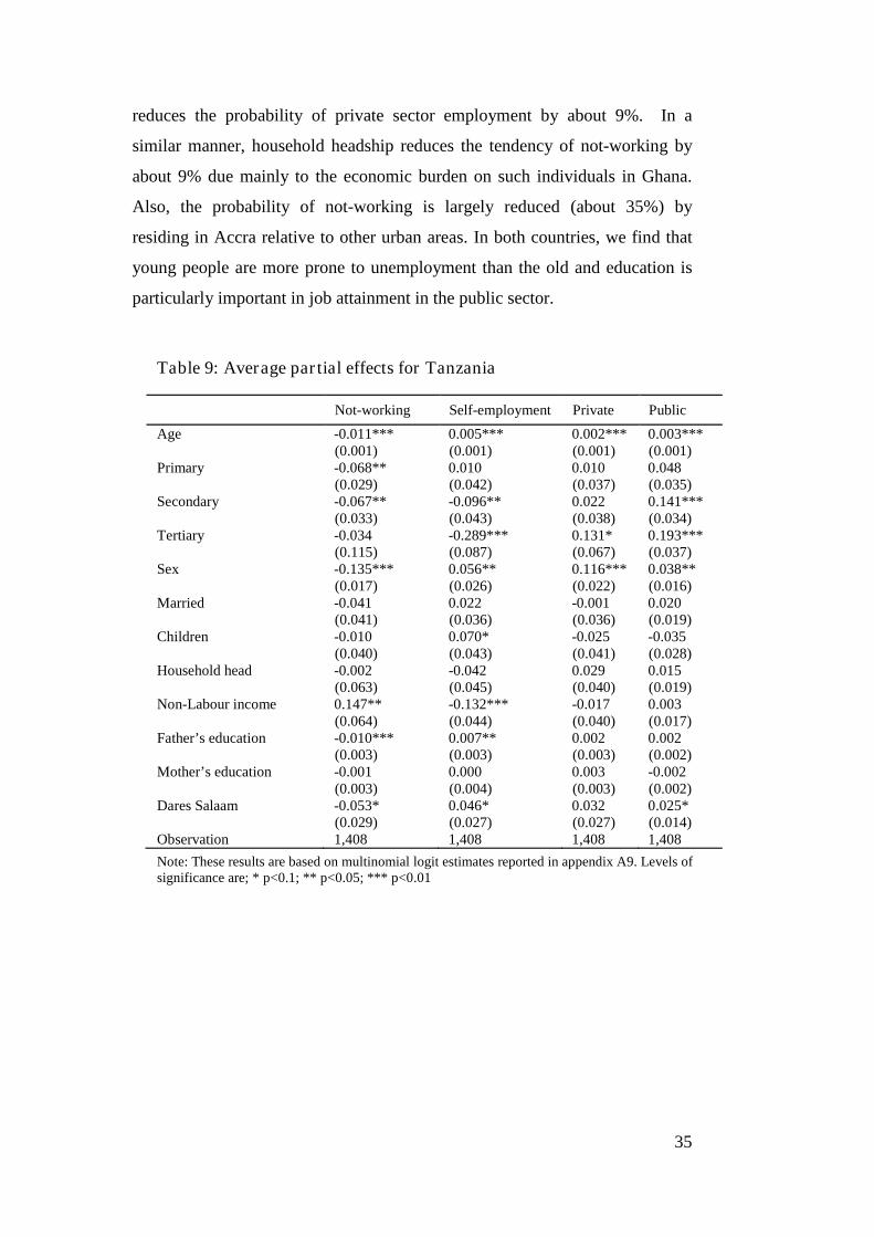
countries are presented in tables 9 and 10.
In Tanzania, age is found increases the probability of participation in all three
employment sectors and decreases the probability of not-working. Having a
primary or secondary education relative to no education reduces the
probability of not-working by about 7% in Tanzania. Secondary and tertiary
education levels reduce the probability of participation in self-employment by
10% and 29% respectively, whereas these levels of education increase the
probability of formal sector employment particularly in the public sector by
14% and 19% accordingly. This is an indication of the existence of preference
for formal sector employment in the Tanzania labour market and the important
role education plays in sector choice. In addition, being a male increase the
probability of employment in all sectors and at reduces not-working
probability. While access to non-labour income increases not-working
probability since such individuals can afford to remain in unemployment due
the availability of resources other than income earned by working. This lends
credence to Appleton et al. (1990) who found asset incomes to have a negative
impact on work decision and participation rates in Cote d’Ivoire. Father’s
education is also found to reduce not-working probability and increase the
probability of self-employment in Tanzania.
In Ghana, average partial effects presented in table 10 highlights a stricter
preference by education for formal sector employment. All levels of education
reduce the likelihood of self-employment in Ghana and increase the
probability of formal sector employment particularly in public sector. Men in
Ghana have increases probability of employment in all sectors and a reduced
probability of not-working. Marriage reduces the probability of not-working
and increases the probability of self-employment whereas access to non-labour
income increases the likelihood of self-employment. This is a reflection of the
phenomenon particularly among low educated women in Ghana who otherwise
would have remained unemployed, are set up in trading by their husbands after
marriage. Having children increases not-working probability by about 8% and
35
reduces the probability of private sector employment by about 9%. In a
similar manner, household headship reduces the tendency of not-working by
about 9% due mainly to the economic burden on such individuals in Ghana.
Also, the probability of not-working is largely reduced (about 35%) by
residing in Accra relative to other urban areas. In both countries, we find that
young people are more prone to unemployment than the old and education is
particularly important in job attainment in the public sector.
Table 9: Average partial effects for Tanzania
Note: These results are based on multinomial logit estimates reported in appendix A9. Levels ofsignificance are; * p<0.1; ** p<0.05; *** p<0.01
Not-working Self-employment Private Public
Age -0.011*** 0.005*** 0.002*** 0.003***(0.001) (0.001) (0.001) (0.001)
Primary -0.068** 0.010 0.010 0.048(0.029) (0.042) (0.037) (0.035)
Secondary -0.067** -0.096** 0.022 0.141***(0.033) (0.043) (0.038) (0.034)
Tertiary -0.034 -0.289*** 0.131* 0.193***(0.115) (0.087) (0.067) (0.037)
Sex -0.135*** 0.056** 0.116*** 0.038**(0.017) (0.026) (0.022) (0.016)
Married -0.041 0.022 -0.001 0.020(0.041) (0.036) (0.036) (0.019)
Children -0.010 0.070* -0.025 -0.035(0.040) (0.043) (0.041) (0.028)
Household head -0.002 -0.042 0.029 0.015(0.063) (0.045) (0.040) (0.019)
Non-Labour income 0.147** -0.132*** -0.017 0.003(0.064) (0.044) (0.040) (0.017)
Father’s education -0.010*** 0.007** 0.002 0.002(0.003) (0.003) (0.003) (0.002)
Mother’s education -0.001 0.000 0.003 -0.002(0.003) (0.004) (0.003) (0.002)
Dares Salaam -0.053* 0.046* 0.032 0.025*(0.029) (0.027) (0.027) (0.014)
Observation 1,408 1,408 1,408 1,408

36
Table 10: Average partial effects for Ghana
Note: results are based on multinomial logit estimates reported in appendix A9. Levels ofsignificance are; * p<0.1; ** p<0.05; *** p<0.01
Not-working
Self-Employment PrivateSector
Public Sector
Age -0.012*** 0.005*** 0.004*** 0.002***(0.001) (0.001) (0.001) (0.001)
Primary -0.029 -0.071*** 0.052* 0.047**(0.023) (0.019) (0.028) (0.022)
Secondary 0.057** -0.164*** 0.042 0.065***(0.027) (0.026) (0.033) (0.023)
Tertiary 0.013 -0.271*** 0.130*** 0.128***(0.039) (0.046) (0.044) (0.024)
Sex -0.019 -0.181*** 0.175*** 0.025**(0.017) (0.017) (0.019) (0.012)
Marriage -0.092*** 0.074*** 0.018 -0.001(0.023) (0.020) (0.027) (0.015)
Children 0.077*** -0.001 -0.094*** 0.018(0.026) (0.024) (0.031) (0.018)
Household head -0.089*** 0.039* 0.056** -0.005(0.023) (0.020) (0.024) (0.012)
Non-Labour income 0.003 0.040** -0.034 -0.008(0.021) (0.019) (0.022) (0.011)
Father’s education 0.008*** -0.002 -0.010** 0.004(0.003) (0.003) (0.004) (0.002)
Mother’s education -0.003 -0.004 0.009** -0.002(0.003) (0.004) (0.004) (0.002)
Accra -0.352*** 0.051*** 0.273*** 0.027***(0.023) (0.017) (0.019) (0.010)
N 2,301 2,301 2,301 2,301
Results with selectivity correction based on the multinomial logit model are
reported in tables 11 and 12. Weighted least squares are applied in the second
stage regression to account for heteroskedasticity present in the model due to
selectivity and standard errors are bootstrap to account for the two stage nature
of the procedure. The results indicate overall, selection bias is not an issue in
the Tanzania sample given that the selection correction term is not significant
in all the three sectors. Similar to Rankin, Sandefur and Teal (2010), no
evidence is found for educational premiums in the public sector. The pattern of
results in the selection corrected model is fairly consistent with the ordinary
least squares results of a positive and convex relationship between education
and earnings particularly in the private sector. In the Tanzania labour market,
being a man in self employment is associated with earnings premium whereas
working in a large firm increases earnings in the private sector.

37
In Ghana, results with sample selection correction are fairly similar to OLS
estimates with a convex earning education relation in private sector. The
selection correction term is however positive and significant in the public
sector but insignificant in the private sector and self-employment. This means
earnings of a worker with average characteristics are higher in this sector than
that of any worker who would be drawn randomly into the public sector.
Conversely, earnings of a worker with average characteristics in either the
private sector or self-employment do not differ significantly from those of a
worker who would be randomly drawn into the sector.
In both countries, we find that education plays an important role in job
attainment particularly in the public sector but within the sector, no evidence
of earnings premium associated with educational levels are found.
Table 11: Selectivity Corrected Earnings Equation Estimates: TanzaniaSelf Private Public
Log of hours 1.017*** -0.269 0.171
(0.145) (0.603) (0.486)
Tenure 0.025 0.022 0.038
(0.017) (0.058) (0.042)
Tenure2 0.000 0.000 -0.001
(0.001) (0.002) (0.001)
Primary 0.660*** 2.633** 0.032
(0.147) (1.188) (0.363)
Secondary 1.172*** 3.511*** 0.462
(0.169) (1.273) (0.503)
Tertiary 0.630*** 4.461*** 0.341
(0.228) (1.199) (0.497)
Sex 0.447*** -0.018 0.105
(0.092) (0.347) (0.318)
Firm size - 0.848*** -
(0.288)
Dare Salaam 0.138 0.316 0.750***
(0.088) (0.328) (0.266)
Selection correction term 0.014 -0.385 0.035
0.225 (0.582) (0.544)
Year dummies Yes Yes Yes
Constant -4.013*** -0.850 2.760
0.817 (3.335) (3.578)Notes: Dependent variable is the log of monthly earnings. Bootstrap standard errors inparenthesis *** p<0.01, ** p<0.05, * p<0.1. Regressions include two year dummies tocontrol for any time specific effects but not included for brevity. Result obtained viaStata Selmlog command.

38
Table 12: Selectivity Corrected Earnings Equation Estimates: GhanaSelf Private Public
Log of hours 0.053 0.091 0.295
(0.204) (0.098) (0.478)
Tenure 0.103*** 0.045 -0.026
(0.038) (0.035) (0.025)
Tenure2 -0.004** 0.000 0.001
(0.001) (0.001) (0.001)
Primary -0.008 0.416** -0.534
(0.147) (0.173) (0.418)
Secondary 0.472** 0.900*** 0.000
(0.227) (0.181) (0.379)
Tertiary 1.413 1.487*** -0.211
(1.125) (0.208) (0.450)
Sex 0.488 0.307** -0.029
(0.319) (0.152) (0.231)
Firm size 0.004*
(0.002)
Accra -0.224 0.042 -0.050
(0.230) (0.162) (0.223)
Selection correction term 0.182 -0.072 0.890*
(0.210) (0.385) (0.536)
Year dummies Yes Yes Yes
Constant 2.918*** 2.451*** 4.545*
(1.042) (0.899) (2.530)Notes: Dependent variable is the log of monthly earnings. Bootstrap standard errors inparenthesis *** p<0.01, ** p<0.05, * p<0.1. Regressions include two year dummies tocontrol for any time specific effects but not included for brevity. Result obtained viaStata Selmlog command.
Heterogeneity in earnings determination
The simple Mincerian earnings equation is based on a restrictive assumption
that the marginal return to education and other earnings determinants are the
same for all individuals. This may not be true in practice since earnings
determinants can vary among individuals due to unobserved factors such as
motivation, ability and initiative. To this end, we examine heterogeneity in
earnings determinants particularly on earnings premiums with educational
levels to determine whether some works benefit more from education than
others and its implications for educational policies and on inequality.
Tables 13 and 14 report regression estimates respectively for the full samples
at three different quantiles, namely, 25th, 50th (median) and 75th of the earnings
distribution for Tanzania and Ghana, OLS results are also reported for
comparison. The results show a consistent pattern with earnings determinants

39
being different at different points in the conditional distribution of earnings. A
test of the null hypothesis of equal covariates effects across quantiles in both
specifications are rejected at 1%; this means all coefficients in the model differ
across quantiles of the earnings distribution, hence the justification for quantile
estimation technique.
Results in table 13 for Tanzania indicate hours of work, tenure, sex and
residence in Dar es Salaam are associated with earnings premium at all
quantiles though not always significant (for tenure and sex at bottom quantile).
Penalties associated with working in the private sector or in self-employment
relative to the public sector are found to be low among the top quantile (75%)
compared to the bottom and median quantiles of conditional earnings
distribution. Similarly, premiums with working in large firms reduce along the
earnings distribution. All educational levels relative to no education as in OLS
estimates, increase earnings along the conditional earnings distribution and
evidence of convex relationship between earnings and education levels are
found at the median and upper quantile of the earnings distribution. The
highest premium to both primary and secondary education in Tanzania is at the
bottom quartile (25th percentile) while that of tertiary level education is largest
at the top quartile (75%) of the conditional earnings distribution. In essence,
we find earnings premium with primary and secondary education to decrease
from the bottom of the earnings distribution to the top whiles the reverse is the
case for tertiary education. We obtain additional support from the F-tests
statistics; the null hypothesis of equality of education level coefficients across
quantiles is rejected for higher against lower quantiles. This is an indication
that among the workers in Tanzania, those with low ability have higher
premiums with primary and secondary education and further suggest these
levels of education are inequality reducing as it lowers the earnings differences
between low and high ability individuals rather than increase it.
In Ghana, hours of work, tenure, sex and residence in Accra increase earnings
along the earnings distribution though not always significantly so at all
quantiles of the conditional earnings distribution (hours of work is significant
at the median and Accra is at the 25th percentile). Firm size premium is highest
at the bottom quantile and decline along the conditional earnings distribution.

40
Table 13: Quantile Regression Estimates for Tanzania
Notes: Dependent variable is the logarithm of monthly earnings. Bootstrap standard errorsin parenthesis *** p<0.01, ** p<0.05, * p<0.1. The F-stat tests the null hypothesis of equalcoefficients (probability of rejecting the null in parenthesis). Regressions include two yeardummies to control for time specific effects but not included for brevity.
OLS 25% 50% 75%Log of hours 0.457*** 0.571*** 0.357** 0.248***
(0.105) (0.202) (0.144) (0.075)Tenure 0.035*** 0.040 0.035* 0.030**
(0.013) (0.027) (0.019) (0.012)Tenure2 -0.000 -0.001 -0.001 -0.000
(0.000) (0.001) (0.000) (0.000)Primary 0.535*** 0.679** 0.397** 0.252**
(0.147) (0.296) (0.200) (0.100)Secondary 0.953*** 1.024*** 0.693*** 0.669***
(0.154) (0.321) (0.179) (0.131)Tertiary 1.218*** 0.794** 0.894** 1.275***
(0.233) (0.351) (0.363) (0.234)Sex 0.030 -0.019 0.179* 0.147***
(0.084) (0.163) (0.092) (0.057)Firm size 0.511*** 0.513*** 0.463*** 0.295**
(0.122) (0.173) (0.103) (0.138)Private -0.759*** -0.838*** -0.677*** -0.458***
(0.121) (0.178) (0.112) (0.115)Self -1.102*** -1.540*** -0.967*** -0.747***
(0.128) (0.242) (0.132) (0.153)Dares Salaam 0.434*** 0.442*** 0.417*** 0.300***
(0.095) (0.151) (0.088) (0.096)Constant 6.924*** 6.691*** 8.126*** 9.249***
(0.600) (1.000) (0.779) (0.433)R2/Pseudo R2 0.278 0.176 0.169 0.202Observations 953 953 953 953
Testing equality ofeducation coefficients:F-Stat (Prob>F)Primary 25% (1, 953) 3.27 (0.0741) 8.27 (0.042)Primary 50% 0.90 (0.342)Secondary 25% 3.82 (0.051) 2.35 (0.126)Secondary 50% 0.02 (0.884)Tertiary 25% 0.11 (0.737) 1.40 (0.238)Tertiary 50% 2.61 (0.107)

41
Table 14: Quantile Regression Estimates for Ghana
Notes: Dependent variable is the logarithm of monthly earnings. Bootstrap standard errors inparenthesis *** p<0.01, ** p<0.05, * p<0.1. The F-stat tests the null hypothesis of equalcoefficients (probability of rejecting the null in parenthesis). Regressions include two yeardummies to control for time specific effects but not included for brevity
OLS 25% 50% 75%Log of hours 0.082 0.110 0.117** 0.038
(0.082) (0.108) (0.055) (0.101)Tenure 0.071*** 0.027 0.038** 0.026*
(0.021) (0.018) (0.017) (0.013)Tenure2 -0.002** -0.000 -0.001 -0.000
(0.001) (0.001) (0.001) (0.000)Primary 0.158 0.143 0.096 0.182**
(0.098) (0.130) (0.074) (0.078)Secondary 0.568*** 0.483*** 0.456*** 0.587***
(0.104) (0.141) (0.071) (0.088)Tertiary 1.071*** 0.730*** 0.975*** 1.205***
(0.126) (0.145) (0.114) (0.079)Sex 0.255*** 0.257*** 0.374*** 0.399***
(0.082) (0.088) (0.050) (0.077)Firm size 0.644*** 0.660*** 0.488*** 0.478***
(0.071) (0.096) (0.073) (0.082)Private -0.042 -0.066 -0.033 0.069
(0.077) (0.104) (0.090) (0.059)Self 0.062 -0.099 0.039 0.277*
(0.130) (0.178) (0.113) (0.157)Accra -0.010 0.115* 0.045 0.025
(0.062) (0.068) (0.049) (0.050)Constant 2.725*** 2.357*** 2.767*** 3.418***
(0.438) (0.653) (0.249) (0.515)R2/Pseudo R2 0.237 0.151 0.160 0.184Observations 1,253 1,253 1,253 1,253
Testing equality ofeducation coefficients:F-Stat (Prob>F)Primary 25% (1, 1248) 0.24 (0.621) 0.16 (0.685)Primary 50% 1.03 (0.312)Secondary 25% 0.06 (0.800) 0.73 (0.392)Secondary 50% 2.44 (0.118)Tertiary 25% 4.58 (0.033) 12.01 (0.071)Tertiary 50% 6.68 (0.010)
All educational levels compared to no education, are associated with earnings
premiums across quantiles in the Ghanaian labour market (though not always
significantly) with larger premiums to high levels of education evident of a
convex relationship between earnings and education. Results from the F-tests
statistics confirm the differential earnings premiums across quantiles. The null
hypothesis of equality of educational level coefficients across quantiles is
rejected for higher against lower quantiles. What emerges from these results is
that, in the Ghanaian labour market, high ability individuals (in the top quartile
42
of the earnings distribution) have more premiums with all levels of education
(primary, secondary and tertiary) compare to low ability earners. Results from
quantile regressions for the different employment sectors are presented in
Tables A11-A16.
5. Conclusion
Identification of the factors that determine earnings in the different labour
market sectors with particular emphasis on the role of education in the various
sectors of employment in urban Tanzania and Ghana was undertaken in this
study with three main objectives; (1) examine the role of education and other
earnings determinants in the labour market by sector of employment; (2)
evaluate the role of education, individual and household characteristics in
selection into the different employment states; and (3) assess the effect of
education and other earnings determinants at different points in the conditional
earnings distribution to determine whether earnings determinants are
homogeneous among workers within countries. Ordinary least squares and
quantile regression techniques were applied, in addition, we attempted to
resolve two main endogeneity issues in the earnings equations which are
omitted variable bias and sample selection bias by the use of instrumental
variables and sample selection correction terms as by Heckman (1979) and Lee
(1983) to achieve the stated objectives.
In both Tanzania and Ghana, we find that education plays an important role in
promoting access to lucrative jobs particularly in the public sector but has no
direct impact on earnings in the public sector. Our results show, a strong
convex education earning relationship is evident in both countries consistent
with Quinn et al, (2008) and Rankin et al, (2010) and particularly so in the
private sector as individuals with high levels of education earn more than those
with low levels of education. We find evidence of sample selection bias within
the public sector in Ghana where individuals positively select themselves into
the sector but no such evidence is found in Tanzania.
Estimated earnings determinants along the earnings distribution indicates
primary and secondary education are inequality-reducing among workers in

43
Tanzania, low ability earners have higher premiums with primary and
secondary education than high ability ones. The situation in the Ghana is, on
the contrary, that high ability earners have higher premiums with primary and
secondary education than low ability ones. In terms of tertiary education, we
find a consistent pattern in both Tanzania and Ghana that it widens earnings
inequality.
The significant sectoral earnings differentials found with OLS are confirmed
by quantile regression estimates on Tanzania. Conditional earnings are lower
in the private sector and in self employment relative to the public sector,
although the gap in earnings is highest at the lower quartile of the earnings
distribution and begins to decrease along the upper tail of the earnings
distribution. However, no such evidence is found for Ghana.
References
Angrist, J. D. And Alan B. Krueger (1991): ‘Does compulsory schoolattendance affect schooling and earnings’, Quarterly Journal of Economics106: 979-1014.
Appleton, S. & Balihuta, A. (1996) “Education and Agricultural Productivity:Evidence from Uganda”. Journal of International Development, 8 (3), 415-444.
Ashenfelter, O., Harmon, C., & Oosterbeek, H. (1999): ‘A review of estimatesof the schooling/earnings relationship, with tests for publicationbias’, Labour economics, 6(4), 453-470.
Becker, G. S. (1964): Human Capital: A Theoretical and Empirical Analysis,with Special Reference to Education, Chicago: University of ChicagoPress.
Beheman, J. (1990): ‘The Action of Human Resource and Poverty on oneanother’, Living Standards Measurement Studies Working Paper 74.Washington, D.C.-World Bank.
Bigsten, A. (1984): ‘Education and income determination in Kenya’, GowerPublishing Company Limited Gower House, Croft Road, Aldershot,England.
Bound, J., Jaeger, D. A. and Becker, M.R. (1995): ‘Problems withInstrumental Variables Estimation when the Correlation between theInstrument and the Endogenous Variables is Weak’, Journal of AmericanStatistical Association 90: 443-450.

44
Bourguignon, F., Fournier, M., and Gurgand, M. (2002): SELMLOG: Satamodule to perfor selection bias correction based on multinomial logitmodel. [online December 2011] available fromhttp://www.crest.fr/pageperso/lmi/gurgand/selmlog.htm.
Bourguignon, F., Fournier, M., and Gurgand, M. (2007): ‘Selection biascorrections based on the multinomial logit model: Monte-Carlocomparisons’, Journal of Economic Surveys, 21(1), 174-205.
Buchinsky M., (1994): ‘Changes in the U.S. Wages Structure 1962-1987:Application of Quantile Regression’ Econometrica 62 405-458.
Card D. (1995b): ‘Using Geographic Variation in College Proximity toEstimate the Return to Schooling’, in Aspects of Labour Market Behaviour:Essays in Honour of John Vanderkamp, ed. by Louis N. Christofides, E.Kenneth Grant and Robert Swidinsky. Toronto: University of TorontoPress (pp. 201-222).
Card, D. (1998): ‘The Causal Effect of Education’, Mimeo, Centre for LabourEconomics, University of California at Berkeley.
Card, D. (2001): ‘Estimating the return to schooling: Progress on somepersistent econometric problems’, Econometrica, 69(5), 1127-1160.
Durbin, J.A. and D. L. McFadden (1984): “An econometric analysis ofresidential electric appliance holdings and consumption”, Econometrica,52: 345-362.
Fields, G.S., (1975): ‘Rural urban migration, urban unemployment andunderemployment, and job-search activity in LDCs’, Journal ofDevelopment Economics 2, no 2, 165-187.
Fitzenberger, B., & Kurz, C. (2003): ‘New insights on earnings trends acrossskill groups and industries in West Germany’, Empirical Economics, 28(3),479-514.
Griliches, Z. and Mason, W. (1972): ‘Education, Income and Ability’, Journalof Political Economy, 80(2), pp. 74-103.
Conneely, K. And Uusitalo, R. (1997): Estimating Heterogeneous TreatmentEffects in the Becker schooling model’, Unpublished discussion paper(Industrial Relations Section, Princeton University).
Griliches, Zvi (1977): ‘Estimating the Returns to Schooling: SomeEconometric Problems’, Econometrica 45: 1-22.
Belzil, C., & Hansen, J. (2004): ‘Earnings dispersion, risk aversion andeducation’, (Vol. 23, pp. 335-358). Emerald Group Publishing Limited.
Harmon, C. and Walker, I. (1995): ‘Estimating the Economic Return ofSchooling for the United Kingdom’, American Economic Review 85: 1278-1286.
Haveman, R. and Wolfe, B. (1984): ‘Schooling and economic well-being: therole of nonmarket effects’, Journal of Human Resources, 19, 377-407.
Heckman, J. J. (1979): ‘Sample selection bias as a specification error’,Econometrica: Journal of the econometric society, 153-161.

45
Heckman, J. and Robb, R.Jr. (1985): ‘Alternative Methods for evaluatingimpact of Interventions: An overview’, Journal of Econometrics, 30(1-2):239-67.
Ichino, A. and Winter-Edmer, R. (1998): ‘The Long-run Educational Cost ofWorld War II’, Unpublished discussion paper (European UniversityInstitute).
Kane, T.J and Rouse C.E (1993): ‘Labour Market Returns to two-and four-year colleges: is a credit to a credit and do degrees matter?’, Working paperno. 4268 (NBER, Cambridge, MA).
Kingdon, G. & Söderbom, M. (2008): ‘Education, Skills, and Labourr MarketOutcomes: Evidence from Ghana’, Working paper series 12. WashingtonDC, World Bank.
Koenker, R. and Bassett G. (1978): ‘Regression quantiles’, Econometrica 46:33-50.
Koenker, R. and Bassett G. (1982): ‘Robust test for heteroskedasticity basedon regression quantiles’, Econometrica 50: 43-61.
Lauer, C. and Steiner, V. (2000): ‘Returns to Education in West Germany –An Empirical Assessment’ ZEW Discussion paper No. 00-04, 2000.
Lee, L. (1983): ‘Generalised Econometric models with selectivity’,Econometrica 51, 507-512.
Machado, JAF. and Mata, J (2000), ‘Sources of increased Wage Inequality’,Mimeo
McFadden, D.L. (1974): ‘Conditional Logit Analysis of Quantitative Choicebehaviour’, in Frontiers in Econometric, ed. By P. Zarembka. New York:Academic Press.
Maluccio, J. (1997): ‘Endogeneity of Schooling in the Wage Function’,Unpublished manuscript (department of Economics, Yale University).
Mincer, J. (1974): ‘Schooling Experience and Earnings’, Columbia UniversityPress: New York.
Mwabu G. and Schultz TP. (1996): ‘Education Returns across Quantiles of theWage function: Alternative explanations for the returns to education byrace in South Africa’, American Economic Review 86(2):334-9.
Skyt Nielsen, H., & Rosholm, M. (2001): ‘The public-private sector wage gapin Zambia in the 1990s: A quantile regression approach’, EmpiricalEconomics, 26(1), 169-182.
Söderbom, M. & Teal, F. (2003): ‘Openness and Human Capital as Sources ofProductivity Growth: An Empirical Investigation’, The Centre for theStudy of African Economies Working Paper Series 188.
Söderbom, M. Teal, F., Wambugu, A. and Kahyarara, G. (2005): ‘TheDynamics of Returns to Education in Kenyan and TanzanianManufacturing’, Global Poverty Research Group Working Paper SeriesGPRG-WPS-017.

46
Strauss, J. and Thomas, D. (1995): ‘Empirical Modelling of HumanResources’, In the handbook of development economics, ed. J. Behrmanand T.N. Srinivasan, 1883-2023. New York: North Holland.
Pradhan, M., A. Van Soest (1995): ‘Formal and Informal Sector Employmentin Urban areas of Bolivia’, Labour Economics, 2:275-97
Psacharopoulos, G. (1994): ‘Returns to Investment in Education: A GlobalUpdate’, World Development 22:9, pp. 1325-1343.
Psacharopoulos, G. and Anthony Patrinos, H. (2002): ‘Returns to investmentin Education: A Further Update’, World Bank Research Paper 2881.Washington D.C: the World Bank.
Quinn S. and Teal F. (2008): ‘Private sector development and incomedynamics: A panel study of the Tanzanian labour market’, CSAEWPS/2008-09.
Rankin N., Sandefur J. and Teal F. (2010): ‘Learning and earning in Africa:Where are the Returns to Education High?’ CSAE WPS/2010-02.
Rogers, W. (1992): ‘Quantile regression standard errors.’ Stata TechnicalBulletin Reprints 3: 77-78
Robert Kivuti Nyaga (2010): ‘Earnings and Employment Sector Choice inKenya’, AERC Research Paper 199.
Schultz, T. W. (1961): ‘Investment in Human Capital’, American EconomicReview, 51 (1), 1-17.
Schultz, T.P. (1999): ‘Health and Schooling Investment in Africa’ Journal ofEconomic Perspectives, 13 (3), 67-88
Todaro, M.P. (1969): ‘A Model of Labour Market Migration and UrbanUnemployment in Less Developed Countries’, American Economic Review39, 138-148
Trost, R.P., and Lee, L. (1984): ‘Technical Training and Earnings: APolychotomous Choice Model with Selectivity’, Review of Economics andStatistics, 66, 151-156
World Bank (1995): ‘Priorities and Strategies for Education: A World BankSector Review’, Washington, D.C: The World Bank, Education and SocialPolicy Department.
Xiaodong, G. and Van Soest, A. (2002): ‘Wage Differentials and Mobilityinto the urban Labour Market: a panel data analysis for Mexico’, LabourEconomics, 9: 513-529.
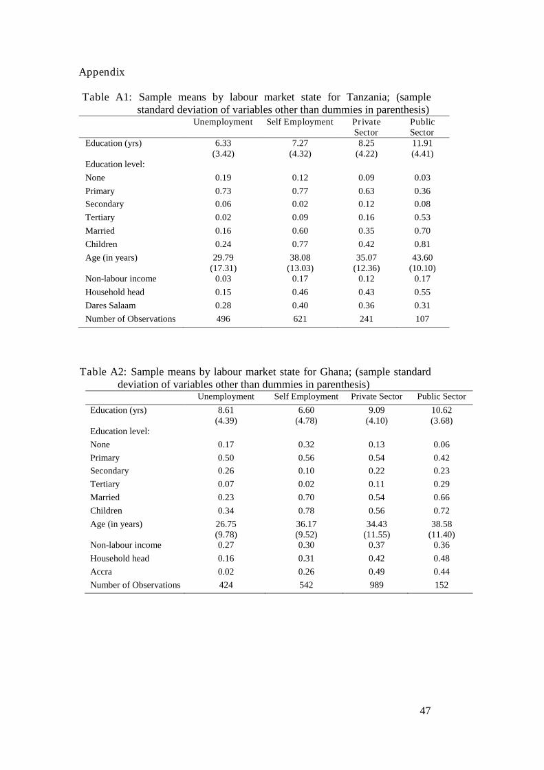
47
Appendix
Table A1: Sample means by labour market state for Tanzania; (samplestandard deviation of variables other than dummies in parenthesis)
Unemployment Self Employment PrivateSector
PublicSector
Education (yrs) 6.33(3.42)
7.27(4.32)
8.25(4.22)
11.91(4.41)
Education level:
None 0.19 0.12 0.09 0.03
Primary 0.73 0.77 0.63 0.36
Secondary 0.06 0.02 0.12 0.08
Tertiary 0.02 0.09 0.16 0.53
Married 0.16 0.60 0.35 0.70
Children 0.24 0.77 0.42 0.81
Age (in years) 29.79(17.31)
38.08(13.03)
35.07(12.36)
43.60(10.10)
Non-labour income 0.03 0.17 0.12 0.17
Household head 0.15 0.46 0.43 0.55
Dares Salaam 0.28 0.40 0.36 0.31
Number of Observations 496 621 241 107
Table A2: Sample means by labour market state for Ghana; (sample standarddeviation of variables other than dummies in parenthesis)
Unemployment Self Employment Private Sector Public Sector
Education (yrs) 8.61(4.39)
6.60(4.78)
9.09(4.10)
10.62(3.68)
Education level:
None 0.17 0.32 0.13 0.06
Primary 0.50 0.56 0.54 0.42
Secondary 0.26 0.10 0.22 0.23
Tertiary 0.07 0.02 0.11 0.29
Married 0.23 0.70 0.54 0.66
Children 0.34 0.78 0.56 0.72
Age (in years) 26.75(9.78)
36.17(9.52)
34.43(11.55)
38.58(11.40)
Non-labour income 0.27 0.30 0.37 0.36
Household head 0.16 0.31 0.42 0.48
Accra 0.02 0.26 0.49 0.44
Number of Observations 424 542 989 152

48
A3: Earnings Equation with years of schooling; Tanzania
Notes: Dependent variable is the log of monthly earnings. Robust standard errors in parenthesis*** p<0.01, ** p<0.05, * p<0.1
Self Private Public Pooled (1) Pooled (2)
Education (yrs) 0.057*** 0.121*** 0.069*** 0.113*** 0.077***
(0.013) (0.019) (0.016) (0.010) (0.010)
Log of hours 0.599*** 0.169 0.860** 0.480*** 0.470***
(0.140) (0.157) (0.369) (0.105) (0.105)
Tenure 0.007 0.081*** 0.049** 0.046*** 0.033***
(0.016) (0.024) (0.019) (0.013) (0.012)
Tenure2 0.000 -0.001** -0.001** -0.000 -0.000
(0.000) (0.001) (0.000) (0.000) (0.000)
Sex 0.106 -0.222 0.033 0.015 0.021
(0.112) (0.162) (0.156) (0.087) (0.084)
Firm size 0.721*** 0.506***
(0.161) (0.120)
Private -0.702***
(0.121)
Self -1.047***
(0.128)
Dares Salaam 0.461*** 0.051 0.491*** 0.398*** 0.427***
(0.122) (0.189) (0.152) (0.099) (0.094)
Year dummies Yes Yes Yes Yes Yes
Constant 5.782*** 7.510*** 5.391*** 5.926*** 7.167***
(0.787) (0.913) (2.034) (0.593) (0.598)
R2 0.127 0.318 0.334 0.199 0.284
Observations 610 238 105 953 953

49
A4: Earnings Equation with years of schooling; Ghana
Notes: Dependent variable is the log of monthly earnings. Robust standard errors in parenthesis*** p<0.01, ** p<0.05, * p<0.1. OLS estimation method
Self Private Public Pooled (1) Pooled (2)
Education (yrs) 0.023* 0.087*** 0.084*** 0.079*** 0.062***
(0.013) (0.011) (0.022) (0.008) (0.008)
Log of hours -0.006 0.142 0.248 -0.009 0.064
(0.199) (0.089) (0.205) (0.085) (0.083)
Tenure 0.106*** 0.042* 0.003 0.060*** 0.070***
(0.033) (0.025) (0.017) (0.020) (0.021)
Tenure2 -0.004*** -0.000 0.000 -0.002* -0.002**
(0.001) (0.001) (0.000) (0.001) (0.001)
Sex 0.361 0.201*** 0.058 0.319*** 0.198**
(0.249) (0.078) (0.110) (0.073) (0.081)
Firm size 0.608*** 0.679***
(0.072) (0.070)
Private -0.108
(0.076)
Self -0.023
(0.127)
Accra -0.250 0.021 0.139 0.041 -0.001
(0.231) (0.069) (0.125) (0.062) (0.062)
Constant 2.988*** 1.906*** 1.924* 3.007*** 2.566***
(1.043) (0.481) (1.087) (0.446) (0.438)
R-squared 0.095 0.278 0.294 0.159 0.216
Observations 387 736 130 1,253 1,253
A5: Earnings equation controlling for endogenous schooling (yrs.); Tanzania
Notes: Dependent variable is the log of monthly earnings. Robust standard errors in parenthesis*** p<0.01, ** p<0.05, * p<0.1. Instrumental variable estimations.
Self Private Public Pooled (1) Pooled (2)Education (yrs) 0.110*** 0.159*** -0.058 0.152*** 0.125***
(0.041) (0.052) (0.089) (0.029) (0.030)Log of hours 0.581*** 0.169 0.580 0.476*** 0.462***
(0.142) (0.149) (0.408) (0.106) (0.105)Tenure 0.007 0.091*** 0.062** 0.043*** 0.034***
(0.017) (0.024) (0.026) (0.013) (0.013)Tenure2 0.000 -0.002*** -0.001** -0.000 -0.000
(0.000) (0.001) (0.001) (0.000) (0.000)Sex -0.008 -0.239 -0.038 -0.039 -0.053
(0.133) (0.159) (0.212) (0.094) (0.090)Firm size 0.700*** 0.480***
(0.176) (0.128)Private -0.520***
(0.166)Self -0.824***
(0.174)Dares Salaam 0.404*** 0.028 0.619*** 0.344*** 0.370***
(0.128) (0.199) (0.200) (0.105) (0.101)Constant 5.524*** 7.155*** 8.513*** 5.679*** 6.650***
(0.858) (0.910) (2.795) (0.650) (0.689)R2 0.098 0.309 0.026 0.178 0.261Observations 571 236 99 906 906

50
A6: Instrumental variable test results for Tanzania
Weak exogeneity testFirst-stage regression summary statistics------------------------------------------------------------------------------------Adjusted Partial RobustVariable R-sq. R-sq. R-sq. F ( 2,893) Prob > F-------------+---------------------------------------------------------------------Education 0.2664 0.2565 0.1049 59.1444 0.0000-----------------------------------------------------------------------------------
Test of exogeneity of instruments (overidentifying restrictions)
Score chi2(1) = .722326 (p = 0.3954)
Hausman test of endogeneity of educationTest: Ho: difference in coefficients not systematic
chi2 (10) = 13.17Prob>chi2 = 0.2144
A7: Instrumental variable test results for Ghana
Weak exogeneity test
First-stage regression summary statistics--------------------------------------------------------------------------------------------Adjusted Partial RobustVariable R-sq. R-sq. R-sq. F (2,1236) Prob > F-------------+----------------------------------------------------------------------------Education 0.2193 0.2117 0.0654 46.5277 0.0000-------------------------------------------------------------------------------------------
Test of exogeneity of instruments (overidentifying restrictions)
Score chi2 (1) = .073593 (p = 0.7862)
Hausman test of endogeneity of educationTest: Ho: difference in coefficients not systematic
chi2 (10) = 19.79Prob>chi2 = 0.0313

51
A8: Earnings equation controlling for endogenous schooling (yrs.); Ghana
Notes: Dependent variable is the log of monthly earnings. Robust standard errors in parenthesis*** p<0.01, ** p<0.05, * p<0.1. Instrumental variable estimations.
Self Private Public Pooled (1) Pooled (2)Education 0.091 0.117*** 0.097 0.119*** 0.106***
(0.062) (0.030) (0.085) (0.021) (0.025)Log of hours -0.042 0.174* 0.234 0.034 0.091
(0.218) (0.096) (0.183) (0.088) (0.084)Tenure 0.095*** 0.041* 0.001 0.062*** 0.067***
(0.033) (0.025) (0.020) (0.020) (0.022)Tenure2 -0.003** -0.000 0.000 -0.002* -0.002**
(0.001) (0.001) (0.001) (0.001) (0.001)Sex 0.164 0.201** 0.083 0.250*** 0.174**
(0.311) (0.079) (0.179) (0.078) (0.080)Firm size 0.547*** 0.591***
(0.094) (0.085)Private -0.061
(0.083)Self 0.103
(0.146)Accra -0.357 0.019 0.141 0.014 -0.010
(0.252) (0.071) (0.123) (0.066) (0.063)Constant 2.861*** 1.501** 1.833 2.472*** 2.039***
(1.098) (0.623) (1.313) (0.518) (0.519)R2 0.024 0.265 0.291 0.134 0.188Observations 385 725 130 1,240 1,240

52
A9: Multinomial logit estimates for Tanzania (Omitted category: Not-working)Self-Employment Private Sector Public Sector
Age 0.337*** 0.326*** 0.697***(0.036) (0.039) (0.095)
Age2 -0.004*** -0.004*** -0.007***(0.000) (0.000) (0.001)
Primary 0.643** 0.589* 1.481**(0.313) (0.344) (0.699)
Secondary 0.387 0.706* 3.111***(0.351) (0.377) (0.697)
Tertiary -0.538 1.077 3.567***(1.159) (1.132) (1.307)
Sex 1.159*** 1.597*** 0.451(0.207) (0.216) (0.356)
Married 0.433 0.314 0.743(0.400) (0.451) (0.525)
Children 0.292 -0.082 -0.487(0.391) (0.450) (0.637)
Household head -0.122 0.183 0.254(0.618) (0.640) (0.695)
Non Labour income -1.629*** -1.187* -1.320*(0.626) (0.648) (0.693)
Father’s education 0.109*** 0.089*** 0.133***(0.032) (0.033) (0.044)
Mother’s education 0.004 0.019 -0.030(0.034) (0.036) (0.050)
Dares Salaam 0.537* 0.551* 0.013(0.288) (0.321) (0.382)
Constant -3.769*** -4.759*** -15.183***(0.933) (1.008) (2.137)
Wald χ2 (D.F) 1187.97 (45)Log-likelihood -1125.82Pseudo-R2 0.35Observations 1,408Standard errors in parenthesis *** Significant at 1% level, ** Significant at 5% level,* Significant at 10% level: Reference categories are; no education, female for sexand Iringa, Arusha, Morogoro, Tanga and Mwanza for region of residence
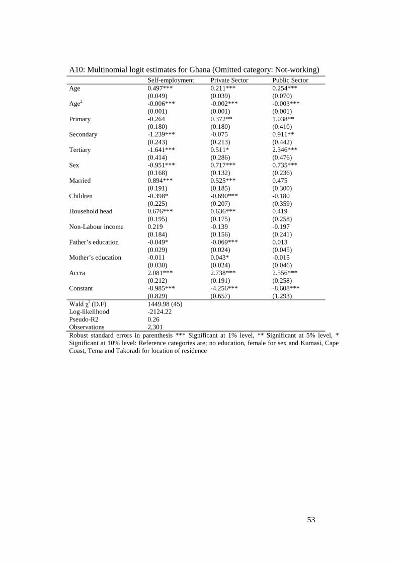
53
A10: Multinomial logit estimates for Ghana (Omitted category: Not-working)
Robust standard errors in parenthesis *** Significant at 1% level, ** Significant at 5% level, *Significant at 10% level: Reference categories are; no education, female for sex and Kumasi, CapeCoast, Tema and Takoradi for location of residence
Self-employment Private Sector Public SectorAge 0.497*** 0.211*** 0.254***
(0.049) (0.039) (0.070)Age2 -0.006*** -0.002*** -0.003***
(0.001) (0.001) (0.001)Primary -0.264 0.372** 1.038**
(0.180) (0.180) (0.410)Secondary -1.239*** -0.075 0.911**
(0.243) (0.213) (0.442)Tertiary -1.641*** 0.511* 2.346***
(0.414) (0.286) (0.476)Sex -0.951*** 0.717*** 0.735***
(0.168) (0.132) (0.236)Married 0.894*** 0.525*** 0.475
(0.191) (0.185) (0.300)Children -0.398* -0.690*** -0.180
(0.225) (0.207) (0.359)Household head 0.676*** 0.636*** 0.419
(0.195) (0.175) (0.258)Non-Labour income 0.219 -0.139 -0.197
(0.184) (0.156) (0.241)Father’s education -0.049* -0.069*** 0.013
(0.029) (0.024) (0.045)Mother’s education -0.011 0.043* -0.015
(0.030) (0.024) (0.046)Accra 2.081*** 2.738*** 2.556***
(0.212) (0.191) (0.258)Constant -8.985*** -4.256*** -8.608***
(0.829) (0.657) (1.293)Wald χ2 (D.F) 1449.98 (45)Log-likelihood -2124.22Pseudo-R2 0.26Observations 2,301

54
A11: Quantile regression estimates with years of schooling for Tanzania
Notes: Dependent variable is the logarithm of monthly earning. Bootstrap standarderrors in parenthesis *** p<0.01, ** p<0.05, * p<0.1.
OLS 25% 50% 75%Log of hours 0.470*** 0.468** 0.350*** 0.268***
(0.105) (0.199) (0.123) (0.061)Tenure 0.033*** 0.042** 0.034** 0.033***
(0.012) (0.020) (0.014) (0.011)Tenure2 -0.000 -0.001 -0.001 -0.001*
(0.000) (0.000) (0.000) (0.000)Education 0.077*** 0.082*** 0.064*** 0.067***
(0.010) (0.017) (0.013) (0.009)Sex 0.021 0.000 0.160 0.157**
(0.084) (0.159) (0.117) (0.061)Firm size 0.506*** 0.537*** 0.418*** 0.314**
(0.120) (0.172) (0.127) (0.150)Private -0.702*** -0.602*** -0.591*** -0.406***
(0.121) (0.165) (0.085) (0.106)Self -1.047*** -1.336*** -0.940*** -0.679***
(0.128) (0.231) (0.125) (0.122)Dares Salaam 0.427*** 0.403*** 0.410*** 0.276***
(0.094) (0.116) (0.098) (0.075)Year dummies Yes Yes Yes YesConstant 6.915*** 7.125*** 8.137*** 8.980***
(0.593) (1.028) (0.768) (0.319)R2/Pseudo R2 0.284 0.176 0.172 0.204Observations 953 953 953 953

55
A12: Quantile regression estimates with years of schooling for Ghana
Notes: Dependent variable is the logarithm of monthly earning. Bootstrap standarderrors in parenthesis *** p<0.01, ** p<0.05, * p<0.1.
OLS 25% 50% 75%Log of hours 0.064 0.145 0.165* 0.085
(0.083) (0.102) (0.090) (0.143)Tenure 0.070*** 0.035*** 0.038*** 0.027*
(0.021) (0.010) (0.014) (0.015)Tenure2 -0.002** -0.000 -0.001 -0.000
(0.001) (0.000) (0.000) (0.000)Education 0.062*** 0.058*** 0.050*** 0.060***
(0.008) (0.012) (0.009) (0.006)Sex 0.198** 0.186*** 0.258*** 0.377***
(0.081) (0.070) (0.054) (0.073)Firm size 0.679*** 0.626*** 0.500*** 0.555***
(0.070) (0.092) (0.057) (0.081)Private -0.108 -0.044 -0.085 -0.024
(0.076) (0.093) (0.092) (0.072)Self -0.023 -0.176 -0.023 0.220**
(0.127) (0.159) (0.120) (0.108)Accra -0.001 0.092 0.032 0.024
(0.062) (0.059) (0.047) (0.042)(0.121) (0.182) (0.115) (0.121)
Year dummies Yes Yes Yes YesConstant 2.698*** 1.868*** 2.447*** 3.088***
(0.436) (0.618) (0.469) (0.754)R2/Pseudo R2 0.216 0.143 0.135 0.143Observations 1,262 1,262 1,262 1,262
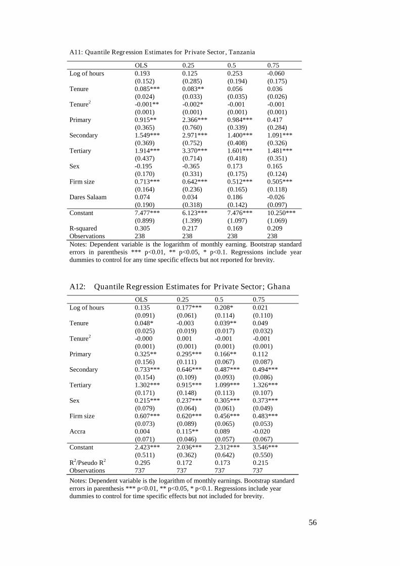
56
A11: Quantile Regression Estimates for Private Sector, Tanzania
Notes: Dependent variable is the logarithm of monthly earning. Bootstrap standarderrors in parenthesis *** p<0.01, ** p<0.05, * p<0.1. Regressions include yeardummies to control for any time specific effects but not reported for brevity.
OLS 0.25 0.5 0.75Log of hours 0.193 0.125 0.253 -0.060
(0.152) (0.285) (0.194) (0.175)Tenure 0.085*** 0.083** 0.056 0.036
(0.024) (0.033) (0.035) (0.026)Tenure2 -0.001** -0.002* -0.001 -0.001
(0.001) (0.001) (0.001) (0.001)Primary 0.915** 2.366*** 0.984*** 0.417
(0.365) (0.760) (0.339) (0.284)Secondary 1.549*** 2.971*** 1.400*** 1.091***
(0.369) (0.752) (0.408) (0.326)Tertiary 1.914*** 3.370*** 1.601*** 1.481***
(0.437) (0.714) (0.418) (0.351)Sex -0.195 -0.365 0.173 0.165
(0.170) (0.331) (0.175) (0.124)Firm size 0.713*** 0.642*** 0.512*** 0.505***
(0.164) (0.236) (0.165) (0.118)Dares Salaam 0.074 0.034 0.186 -0.026
(0.190) (0.318) (0.142) (0.097)Constant 7.477*** 6.123*** 7.476*** 10.250***
(0.899) (1.399) (1.097) (1.069)R-squared 0.305 0.217 0.169 0.209Observations 238 238 238 238
A12: Quantile Regression Estimates for Private Sector; Ghana
Notes: Dependent variable is the logarithm of monthly earnings. Bootstrap standarderrors in parenthesis *** p<0.01, ** p<0.05, * p<0.1. Regressions include yeardummies to control for time specific effects but not included for brevity.
OLS 0.25 0.5 0.75Log of hours 0.135 0.177*** 0.208* 0.021
(0.091) (0.061) (0.114) (0.110)Tenure 0.048* -0.003 0.039** 0.049
(0.025) (0.019) (0.017) (0.032)Tenure2 -0.000 0.001 -0.001 -0.001
(0.001) (0.001) (0.001) (0.001)Primary 0.325** 0.295*** 0.166** 0.112
(0.156) (0.111) (0.067) (0.087)Secondary 0.733*** 0.646*** 0.487*** 0.494***
(0.154) (0.109) (0.093) (0.086)Tertiary 1.302*** 0.915*** 1.099*** 1.326***
(0.171) (0.148) (0.113) (0.107)Sex 0.215*** 0.237*** 0.305*** 0.373***
(0.079) (0.064) (0.061) (0.049)Firm size 0.607*** 0.620*** 0.456*** 0.483***
(0.073) (0.089) (0.065) (0.053)Accra 0.004 0.115** 0.089 -0.020
(0.071) (0.046) (0.057) (0.067)Constant 2.423*** 2.036*** 2.312*** 3.546***
(0.511) (0.362) (0.642) (0.550)R2/Pseudo R2 0.295 0.172 0.173 0.215Observations 737 737 737 737

57
A13: Quantile Regression Estimates for Public Sector, Tanzania
OLS 0.25 0.5 0.75Log of hours 0.828** 0.509 0.447 0.505
(0.398) (0.377) (0.371) (0.319)Tenure 0.058*** 0.068*** 0.047* 0.049
(0.019) (0.018) (0.024) (0.031)Tenure2 -0.001*** -0.002*** -0.001 -0.001
(0.000) (0.001) (0.001) (0.001)Primary 0.059 -0.306 -0.064 0.137
(0.230) (0.232) (0.276) (0.246)Secondary 0.631*** 0.328 0.719** 0.755***
(0.157) (0.216) (0.282) (0.178)Tertiary 0.676*** 0.224 0.578* 0.914**
(0.236) (0.210) (0.313) (0.416)Sex 0.047 0.167 0.051 0.122
(0.172) (0.210) (0.167) (0.128)Dares Salaam 0.505*** 0.318*** 0.202 0.393
(0.169) (0.115) (0.197) (0.284)Constant 5.870** 7.812*** 8.215*** 7.910***
(2.346) (2.464) (2.260) (1.810)R-squared 0.312 0.240 0.168 0.153Observations 105 105 105 105Notes: Dependent variable is the logarithm of monthly earning. Bootstrapstandard errors in parenthesis *** p<0.01, ** p<0.05, * p<0.1. Regressionsinclude year dummies to control for any time specific effects but not reported forbrevity.
A14: Quantile Regression Estimates for Public Sector, Ghana
Notes: Dependent variable is the logarithm of monthly earning. Bootstrapstandard errors in parenthesis *** p<0.01, ** p<0.05, * p<0.1. Regressionsinclude year dummies to control for any time specific effects but not reported forbrevity
OLS 0.25 0.5 0.75Log of hours 0.243 0.410 0.391 0.316
(0.222) (0.248) (0.348) (0.222)Tenure -0.004 -0.011 -0.019 -0.017
(0.017) (0.026) (0.022) (0.026)Tenure2 0.001 0.001 0.001 0.001
(0.000) (0.001) (0.001) (0.001)Primary -0.000 0.157 0.401 0.327
(0.345) (0.227) (0.525) (0.717)Secondary 0.498 0.535* 0.940 0.859
(0.354) (0.308) (0.583) (0.708)Tertiary 0.664* 0.955*** 1.197** 1.133
(0.379) (0.317) (0.550) (0.725)Sex 0.109 -0.005 0.147 0.396***
(0.121) (0.127) (0.128) (0.117)Accra 0.122 0.072 0.139 0.227**
(0.124) (0.173) (0.114) (0.111)Constant 3.300*** 2.267* 2.080 2.579***
(1.219) (1.191) (1.764) (0.961)R-squared 0.307 0.193 0.251 0.314Observations 130 130 130 130

58
A15: Quantile Regression Estimates for Self-employment, Tanzania
Notes: Dependent variable is the logarithm of monthly earning. Bootstrap standarderrors in parenthesis *** p<0.01, ** p<0.05, * p<0.1. Regressions include yeardummies to control for any time specific effects but not reported for brevity.
OLS 0.25 0.5 0.75Log of hours 0.579*** 0.849*** 0.413* 0.309***
(0.140) (0.317) (0.227) (0.083)Tenure 0.006 0.001 0.016 0.026*
(0.016) (0.017) (0.020) (0.016)Tenure2 0.000 0.000 -0.000 -0.001
(0.000) (0.000) (0.001) (0.000)Primary 0.444*** 0.532 0.334** 0.188
(0.169) (0.358) (0.157) (0.154)Secondary 0.669*** 0.675** 0.374* 0.445***
(0.184) (0.313) (0.192) (0.160)Tertiary 1.113** 0.543 0.672 1.349*
(0.464) (0.826) (0.905) (0.704)Sex 0.124 0.065 0.180** 0.206**
(0.111) (0.120) (0.085) (0.097)Dares Salaam 0.465*** 0.605*** 0.551*** 0.364***
(0.122) (0.219) (0.170) (0.089)Constant 6.103*** 4.219** 6.851*** 7.933***
(0.750) (1.745) (1.148) (0.457)R-squared 0.123 0.107 0.064 0.081Observations 610 610 610 610
A16: Quantile Regression Estimates for Self-employment, Ghana
Notes: Dependent variable is the logarithm of monthly earning. Bootstrap standarderrors in parenthesis *** p<0.01, ** p<0.05, * p<0.1. Regressions include yeardummies to control for any time specific effects but not reported for brevity.
OLS 0.25 0.5 0.75Log of hours 0.027 0.191 -0.039 -0.271
(0.191) (0.302) (0.122) (0.364)Tenure 0.109*** 0.067** 0.079*** 0.054*
(0.033) (0.031) (0.010) (0.031)Tenure2 -0.004*** -0.002* -0.002*** -0.001
(0.001) (0.001) (0.000) (0.001)Primary -0.015 -0.174 -0.033 0.214
(0.132) (0.149) (0.098) (0.140)Secondary 0.406** 0.233 0.246 0.578***
(0.186) (0.215) (0.170) (0.186)Tertiary 1.244 0.098 1.079 0.715
(1.090) (1.146) (1.601) (1.961)Sex 0.354 0.801*** 0.529*** 0.618***
(0.245) (0.194) (0.094) (0.208)Accra -0.206 -0.409 0.013 0.025
(0.232) (0.398) (0.280) (0.297)Constant 2.982*** 1.778 3.378*** 4.943**
(0.962) (1.464) (0.613) (1.982)R-squared 0.107 0.057 0.067 0.070Observations 386 386 386 386

59