Detection and Tracking the VanishingPoint on the Horizon

Young-Woo Seo

CMU-RI-TR-14-07

May 2014

The Robotics InstituteCarnegie Mellon University

Pittsburgh, Pennsylvania 15213

c© Carnegie Mellon University

AbstractIn advanced driver assistance systems and autonomous driving vehicles, many

computer vision applications rely on knowing the location of the vanishing point ona horizon. The horizontal vanishing point’s location provides important informationabout driving environments, such as the instantaneous driving direction of roadway,sampling regions of the drivable regions’ image features, and the search direction ofmoving objects. To detect the vanishing point, many existing methods work frame-by-frame. Their outputs may look optimal in that frame. Over a series of frames, however,the detected locations are inconsistent, yielding unreliable information about roadwaystructure. This paper presents a novel algorithm that, using line segments, detects van-ishing points in urban scenes and, using Extended Kalman Filter (EKF), tracks themover frames to smooth out the trajectory of the horizontal vanishing point. The studydemonstrates both the practicality of the detection method and the effectiveness of ourtracking method, through experiments carried out using thousands of urban scene im-ages.

I

Contents1 Introduction 1

2 A Bayes Filter for Tracking a Vanishing Point on the Horizon 22.1 Vanishing Point Detection . . . . . . . . . . . . . . . . . . . . . . . 32.2 Vanishing Point Tracking . . . . . . . . . . . . . . . . . . . . . . . . 4

3 Experiments 9

4 Conclusions and Future Work 10

5 Acknowledgments 11

III

Figure 1: Sample images show the necessity of a vanishing point tracking for real-world, automotive applications. The red circle represents the vanishing points detectedfrom the input images and the green circle represents the vanishing points tracked overframes. The yellow line represents the estimated horizon line. The existing, frame-by-frame vanishing point detection methods would fail when relevant image features arenot present at the input images.

1 IntroductionThis paper presents a simple, but effective method for detecting and tracking the van-ishing point on a horizon appearing in a stream of urban scene images. In urban streetscenes, such detecting and tracking would enable the obtaining of geometric cues of 3-dimensional structures. Given the image coordinates of the horizontal vanishing point,one could obtain, in particular, the information about the instantaneous driving direc-tion of a roadway [5, 11, 14, 16, 17, 18, 20, 21], the information about the imageregions for sampling the features of the drivable image regions [13, 15], the searchdirection of moving objects [12], and computational metrology through homography[19]. Advanced driving assistance systems or self-driving cars can exploit such infor-mation to detect neighboring moving objects and decide where to drive. Such infor-mation about roadway geometry can be obtained using active sensors (e.g., lidars withmulti-horizontal planes or 3-dimensional lidar [23]), but, as an alternative, many re-searchers have studied the use of vision sensors, due to lower costs and flexible usages[1, 2, 5, 12].

A great deal of excellent work has been done in detecting vanishing points on per-spective images of man-made environments; their performances are demonstrated oncollections of images [3, 4, 10, 22]. Most of these methods, in voting on potentiallocations of vanishing points, use low-level image features such as spatial filter re-sponses (e.g., Garbor filters) [15, 11, 18, 25] and geometric primitives (e.g., lines)[10, 19, 21, 22]. To find an optimal vote result, the methods use an iterative algorithmsuch as Expectation and Maximization (EM).

However, these frame-by-frame vanishing point detection methods may be imprac-tical for real-time, automotive applications primarily because 1) they require inten-sive computation per frame and 2) they expect a presence of low-level image features.

1

In particular, it may take longer than a second simply to apply spatial filters to largeparts of or the entire input image. Meanwhile, a vehicle drives a number of meterswith no information about road geometry. Furthermore, these frame-by-frame meth-ods would fail to detect the vanishing point appearing on over- and under-exposed im-ages. Such images are acquired when a host-vehicle is emerging from tunnels or over-passes. Figure 1 (b) shows a sample image acquired when our vehicle emerges froma tunnel. When this happens, these methods would fail to continuously provide infor-mation about the vanishing point’s location. Because of such a practical issue, someresearchers developed Bayes filters to track the vanishing point’s trajectory [15, 21]. Inaddition to the two aforementioned concerns, we have one of our own. In an earlierwork [19], we demonstrated the ability to acquire, using a monocular camera sensor,the information of a vehicle’s lateral motions as well as metrological information ofthe ground plane. To correctly compute metric information such as lateral distances ofa vehicle to both boundaries of the host road-lane, it is critical to accurately estimatethe angle between the road plane and the camera plane. To do this, we detect the van-ishing point on the horizon to estimate the angle between two planes. But, because,image features relevant to detecting the vanishing point are missing in certain frames,our vanishing point detection fails to correctly locate the vanishing point, resulting inincorrect angle measurements and distance computations.

To address these practical concerns, we have developed a novel method of detectingand tracking the vanishing point on the horizon. In what follows, Section 2.1 detailshow we extract line segments from an input image and how we detect, using extractedline segments, the vanishing point on the horizon. Section 2.2 describes our imple-mentation of Extended Kalman Filter (EKF) for tracking the detected vanishing point.Section 3 explains experiments conducted to demonstrate the effectiveness of the pro-posed algorithms and discusses the findings. Finally Section 4 lays out our conclusionsand future work.

The contributions of this paper include 1) a method, based on line segments, forfast detection of vanishing points, 2) a novel vanishing point tracking algorithm basedon a Bayes filter, and 3) empirical validations of the proposed work.

2 A Bayes Filter for Tracking a Vanishing Point on theHorizon

This section details our approach to the problem of detecting and tracking a vanishingpoint on a horizon, in particular, on perspective images of urban streets. A vanishingpoint on a perspective image is the intersection point of two parallel lines. In urbanstreet scenes, as long as the image is under normal exposure, one can obtain plenty ofparallel line pairs, pairs such as longitudinal lane-markings and building contour lines.Section 2.1 describes how we extract lines and, with them, detect vanishing points.The image coordinates of the vanishing points detected from individual frames maybe temporally inconsistent because lines relevant to and important for vanishing pointdetection may not have been extracted. To smooth out the location of vanishing pointsover time, we develop an extended Kalman filter to track vanishing points. Section 2.2

2

Figure 2: (a) A prior for the line classification. (b) An example of line detection andclassification. The red (blue) lines are categorized into the vertical (horizontal) linegroup. The yellow, dashed rectangle represents a ROI for line extraction.

details the procedure and measurement model of our EKF implementation.

2.1 Vanishing Point Detection

Our algorithm detects, by using line segments, vanishing points appearing on a per-spective image. In an urban scene image, one can extract numerous lines from urbanstructures, like man-made structures (e.g., buildings, bridges, overpasses, etc.) and traf-fic devices (e.g., Jersey barriers, lane-markings, curbs, etc.) To obtain these lines, wetried three line-extraction methods: Kahn’s [9, 10], the probabilistic, and the standardHough transform [6]. We found Kahn’s method to work best in terms of the num-ber of resulting lines and their geometric properties, such as lengths or representationfidelity to the patterns of low-level features. To implement Kahn’s method, we firstobtain Canny edges and run the connected component-grouping algorithm to producea list of pixel blobs. For each pixel blob, we compute the eigenvalues and eigenvectorsof the pixel coordinates’ dispersion matrix. The eigenvector, e1, associated with thelargest eigenvalue is used to represent the orientation of a line segment and its length,lj = (θj , ρj) = (atan2(e1,2, e1,1), x cos θ+ y sin θ), where x = 1

nΣkxk, y = 1nΣkyk.

The two parameters, θj and ρj , are used to determine two end points, p1j =

[x1j , y

1j

]and p2

j =[x2j , y

2j

], of the line segment lj . Figure 2 (b) shows an example of line

detection result.Given a set of the extracted lines, L = {lj}j=1,...,|L|, we first categorize them into

one of two groups: vertical LV or horizontal LH , L = LV ∪LH . We do this to use onlya relevant subset of the extracted lines for detecting a particular (vertical or horizontal)vanishing point. For example, if vertical lines were used to find a horizontal vanishingpoint, the coordinates of the resulting vanishing point would be far from optimal. Toset the criteria for this line categorization, we define two planes: h = [0, 0, 1]

T fora horizontal plane and v = [0, 1, 0]

T for a vertical plane in the camera coordinate.We do this because we assume that the horizontal (or vertical) vanishing points lie

3

at a horizontal (or vertical) plane at the front of our vehicle. Figure 2 (a) illustratesour assumption about these priors. We transform, the coordinates of the extractedline segments’ two points into those of the camera coordinates, pcam = K−1pim,where pcam is a point in the camera coordinates, K is the camera calibration matrixof intrinsic parameters, and pim is a point in the image coordinates. We then computethe distance of a line segment, lj = [aj , bj , cj ]

T ,1 to the horizontal, h, and the verticalplane, v. We assign a line to either of two line groups based on the following:

LV ← lj , if lTj · v ≤ lTj · h, (1)LH ← lj , Otherwise

where lTj ·v =[aj ,bj ,cj ]

T [0,1,0]√a2j+b

2j+c

2j

. Figure 2 (b) shows an example of line classification re-

sult; vertical lines are depicted in red, horizontal lines in blue. Such line categorizationresults help us use a subgroup of the extracted lines relevant to computing the verticalor horizontal vanishing point. Our approach of using line segments to detect vanish-ing point is similar to some found in earlier work [10, 21, 22]. All uses line segments(or edges) to detect vanishing points. Our distinguishes itself in terms of line classi-fication. Suttorp and Bucher’s method relied on a heuristic, to cluster lines into leftor right sets for vanishing point detection [21]; Tardif [22] used a J-linkage algorithmto group edges into the same clusters. In contrast, our method distinguishes horizontalline segments from vertical ones by setting priors about the ideal locations of vanishingpoints.

Given two sets of line groups (vertical and horizontal), we run RANSAC [6] tofind the best estimation of a vanishing point. For each line pair randomly selectedfrom the horizontal and vertical line groups, we first compute the cross-product of twolines, vpij = li × lj , to find an intersection point. The intersection point found thusis used as a vanishing point candidate. We then claim the vanishing point candidatewith the smallest number of outliers as the vanishing point for that line group. A linepair is regarded as an outlier if the angle between a vanishing point candidate and thevanishing point obtained from the line pair is greater than a pre-defined threshold (e.g.,5 degrees). We repeat this procedure until a vertical vanishing point is found and morethan one horizontal vanishing point is obtained. The horizontal vanishing point withthe smallest number of outliers is selected as the vanishing point on the horizon. Figure3 shows sample results of vanishing point detection.

2.2 Vanishing Point Tracking

The previous section detailed how we detect vanishing points using line segments ex-tracted from urban structures. Such frame-by-frame detection results, however, maybe inconsistent over frames. This is because some image features (i.e., line segments)relevant to detecting vanishing points on the previous frame may not be available inthe current frame. When this happens, any frame-by-frame, vanishing point detection

1Using two end-points of a line segment, we can represent a line segment in an implicit line equation,where, aj = y1j − y2j , bj = x2

j − x1j , c = x1

jy2j − x2

jy1j .

4

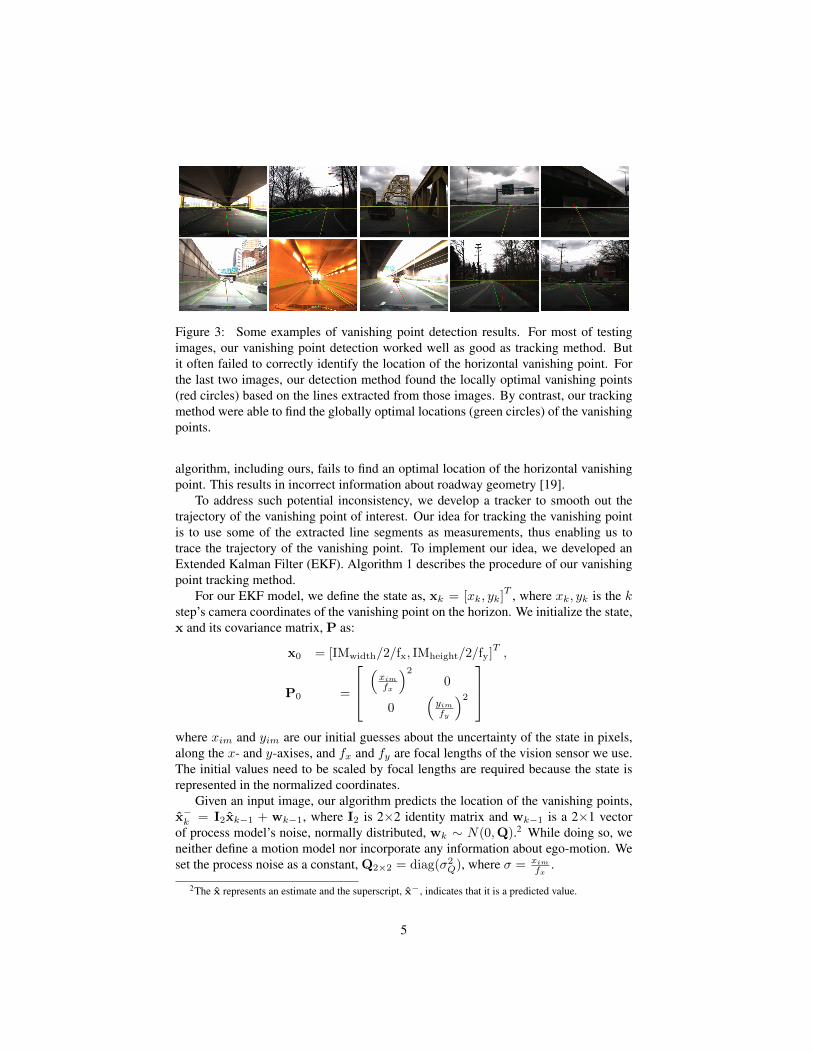
Figure 3: Some examples of vanishing point detection results. For most of testingimages, our vanishing point detection worked well as good as tracking method. Butit often failed to correctly identify the location of the horizontal vanishing point. Forthe last two images, our detection method found the locally optimal vanishing points(red circles) based on the lines extracted from those images. By contrast, our trackingmethod were able to find the globally optimal locations (green circles) of the vanishingpoints.

algorithm, including ours, fails to find an optimal location of the horizontal vanishingpoint. This results in incorrect information about roadway geometry [19].

To address such potential inconsistency, we develop a tracker to smooth out thetrajectory of the vanishing point of interest. Our idea for tracking the vanishing pointis to use some of the extracted line segments as measurements, thus enabling us totrace the trajectory of the vanishing point. To implement our idea, we developed anExtended Kalman Filter (EKF). Algorithm 1 describes the procedure of our vanishingpoint tracking method.

For our EKF model, we define the state as, xk = [xk, yk]T , where xk, yk is the k

step’s camera coordinates of the vanishing point on the horizon. We initialize the state,x and its covariance matrix, P as:

x0 = [IMwidth/2/fx, IMheight/2/fy]T,

P0 =

(xim

fx

)20

0(yimfy

)2

where xim and yim are our initial guesses about the uncertainty of the state in pixels,along the x- and y-axises, and fx and fy are focal lengths of the vision sensor we use.The initial values need to be scaled by focal lengths are required because the state isrepresented in the normalized coordinates.

Given an input image, our algorithm predicts the location of the vanishing points,x−k = I2xk−1 + wk−1, where I2 is 2×2 identity matrix and wk−1 is a 2×1 vectorof process model’s noise, normally distributed, wk ∼ N(0,Q).2 While doing so, weneither define a motion model nor incorporate any information about ego-motion. Weset the process noise as a constant, Q2×2 = diag(σ2

Q), where σ = xim

fx.

2The x represents an estimate and the superscript, x−, indicates that it is a predicted value.

5

Algorithm 1 EKF for tracking the vanishing point.Require: IM, an input image and L, a set of line segments extracted from the input

image, {lj}j=1,...,|L| ∈ LEnsure: xk = [xk, yk]

T , an estimate of the image coordinates of the vanishing pointon the horizon

1: Detect a vanishing point, vph = Detect(IM, L)2: Run EKF iff vphx ≤ IMwidth and vphy ≤ IMheight. Otherwise exit.3: EKF: Prediction4: x−k = f(xk−1) + wk−15: Pk = Fk−1Pk−1F

Tk−1 + Qk−1

6: EKF: Measurement Update7: for all lj ∈ L do8: yj = zj − h(x−k )9: Sj = HjPjH

Tj + Rj

10: Kj = PjHTj S−1j

11: Update the state estimate if yj ≤ τ12: xk = x−k + Kj yj13: Pj = (I2 −KjHj)Pj14: end for

For the measurement update, we first change the representation of an extractedline segment, lj , as a pair of image coordinates of its mid-point and orientation, lj =

[mj , θj ]T , where θj ∈

[−π2 ,

π2

],mj = [mj,x,mj,y]T . Note that the line segments we

use as measurements for EKF are the same ones that used for detecting the vanishingpoint. Our approach is similar to Suttorp and Bucher’s method [21], but both employdifferent measurement models. We then compute the residual, yj , the difference be-tween our expectation on an observation, h(x−k ) and an actual observation zj = θj .

We presume that if a selected line segment, lj , is aligning with the vanishing pointof interest, xk = [xk, yk]

T , the angle between the vanishing point and the orientationof the line should be zero (or very close to zero). Figure 5 illustrates the underlyingidea of our measurement model that investigates the geometric relation between anextracted line and a vanishing point of interest. Based on this idea, we design a modelof what we expect to observe, our observation model, as

h(xk) = tan−1(yk −mj,y

xk −mj,x

)(2)

To linearize this non-linear observation model, we take the first-order, partial derivativeof h(xk), with respect to the state, xk, to derive the Jacobian of the measurementmodel, H.

∂h(xk)

∂x=

[−(yk −mj,y)

d2,

(xx −mj,x)

d2

]= H (3)

where d2 =√

(xk −mj,x)2 + (yk −mj,y)2. We set the measurement noise, vk ∼

6

Figure 4: A comparison of vanishing point locations by the frame-by-frame detectionand by the EKF tracking.

N(0,R) and R1×1 = σ2R, where σ = 0.1 radian. We then compute the innovation Sj

and the Kalman gain Kj for the measurement update.Before actually updating the state using these measurements, we treat individual

line segments differently based on their lengths. This is because the shorter the lengththe higher the chance of the line being a noise measurement.3 To implement this idea,we compute a weight of the line based on its length and heading difference, to updatethe measurement noise.

R = Rmax +

(Rmin −Rmaxlmax − lmin

)|lj | (4)

where Rmax (e.g., 10 degrees) and Rmin (e.g., 1 degree) define the maximum andthe minimum of heading difference in degree, and lmax (e.g., 500) and lmin (e.g., 20)define the maximum and minimum of observable line lengths in pixels, |lj | is the lengthof the line. This equation ensures that we treats the longer line more importantly whenupdating the state and we only use lines of which heading differences are smaller thanthe threshold, τ .

In summary, the task of our EKF is to analyze line measurements to estimate thelocation of the vanishing point on the horizon. Figure 4 shows some example resultsthat one can see the difference of the locations between the detected and the trackedvanishing points.4

We use the tracked vanishing point to compute the (pitch) angle between the cameraplane and the ground plane. The underlying assumption is that the vanishing pointalong the horizon line is exactly mapped to the camera center if the road plane is flatand perpendicular to an image plane. From this assumption, we can derive the locationof the vanishing point on the horizon line as [8]:

vp∗h(φ, θ, ψ) =

[cφsψ − sφsθcψ

cθcψ,−sφsψ − cφsθcψ

cθcψ

]T(5)

3Recall that we extract line segments from Canny’s edge image where short edges may originate fromartificial patterns, not from actual objects’ contours.

4Some of the vanishing point tracking videos are available from, http://www.cs.cmu.edu/˜youngwoo/research.html

7

Figure 5: The line measurement model. The red circle represents the vanishing point,xk, tracked until kth step. θj is the orientation of the jth line, lj , and β is the orientationbetween the line’s mid-point and the vanishing point. The orientation difference is theresidual of our EKF model.

where φ, θ, ψ are yaw, pitch, and roll angle of the camera plane with respect to theground plane and c and s for cos and sin. Since we are interested in estimating thepitch angle, let us suppose that there is no vertical tilt and rolling (i.e., the yaw and theroll angles are zero). Then the above equation yields:

vp∗h(φ = 0, θ, ψ = 0) =

[0

cθ,−sθ

cθ

](6)

Because we assume that there is neither yaw nor roll, we can compute the pitch angleby computing the difference between the y-coordinate of the vanishing point and thatof the principal point of the camera as

θ = tan−1 (|py − vpy|) (7)

where py is the y coordinate of the principal point. Figure 6 shows our setup to verifythe accuracy of our pitch angle estimation. Because no precise angle measurementexists between the two planes, we instead measure the distances between the cameraand markers on the ground to evaluate the accuracy of the pitch angle computation. Wefound that the distance measurements have, on average, a sub-meter accuracy (i.e., lessthan 30cm).

8

Figure 6: A setup for verifying the accuracy of our world-coordinate computationmodel. The intersection point of the two red lines represents the camera center and theintersection point of the two green lines represents a vanishing point computed fromthe two blue lines appearing on the ground.

3 Experiments

To evaluate the performance of our vanishing point detection and tracking algorithm,we drove our robotic car [24] on a route of inter-city highways, to collect some imagedata and the vehicle’s ego-motion data. Our vehicle is equipped with a military-gradeIMU which, in root-mean-square sense, the error of pitch angle estimation is 0.02 withGPS signals (with RTK corrections) or 0.06 degree with GPS outage, when drivingmore than one kilometer or for longer than one minute. The vision sensor installed onour vehicle is PointGrey’s Flea3 Gigabit camera, which can acquire an image frameof 2448×2048, maximum resolution at 8Hz. While driving the route, we ran the pro-posed algorithms as well as the data (i.e., image and vehicle states) collector. Weimplemented the proposed methods in C++ and OpenCV that runs about 20Hz. Thedata collector automatically syncs the high-rate, ego-motion data (i.e., 100Hz) with thelow-rate, image data (i.e., 8Hz). To estimate the camera’s intrinsic parameters, we useda publicly, available toolbox for camera calibration5 and define a rectangle for the lineextraction ROI, x1 = 0, x2 = Iwidth−1, y1 = 1300 and y2 = 1800. We empiricallyfound that Rmax = 10, Rmin = 1, lmax = 500, and lmin = 20 worked best.

5http://www.vision.caltech.edu/bouguetj/calib_doc/

9

Figure 7: A comparison of the estimated pitch angles by an IMU and by the proposedmethod.

We evaluated quantitatively and qualitatively the performance of the presented van-ishing point tracking method.

For the quantitative evaluation, we analyzed the accuracy of the pitch angles esti-mated from the vanishing point tracking. Figure 7 shows the comparison of the pitchangles measured by the IMU and estimated by a monocular vision sensor. Althoughthe pitch angles estimated from our algorithm have some periods underestimate thetrue pitch angles, the two graphs have, at a macro-level, similar shapes where the bluecurve follows the ups-and-downs of the red curve. The mean-square error is 2.0847degrees.

For the qualitative evaluation, we analyzed how useful the output of the trackedvanishing point is in approximating the driving direction of a road way. Figure 8 showssome example results that, within a certain range, the driving directions of roads can belinearly (or instantaneously) approximated by linking the locations of the tracking van-ishing point to the center of the image bottom (i.e., the image coordinates our camerais projected on).

4 Conclusions and Future Work

This paper has presented a novel method of detecting vanishing points and of track-ing a vanishing point on the horizon. To detect vanishing points, we extracted linesand applied RANSAC to the locally optimal vanishing point from a given input im-age. Occasionally, however, our method failed to detect the vanishing point becauserelevant image features were unavailable. Our previous computer vision applicationfor autonomous driving required metric computation to accurately measure the vehi-cle’s lateral motion. To obtain this measurement, one needs an accurate measurementof the angle between the camera and the ground planes. To compute this angle, weused the detected vanishing point. Thus, when the vanishing point location was inac-

10

Figure 8: This figure shows the idea of using results of vanishing point detection toapproximate the driving direction of a roadway. We used such approximated drivingdirections to remove false-positive lane-marking detections [20]. The green blobs arethe final outputs of lane-marking detection and the red blobs are the false-positive lane-marking detections that are removed from the final results.

curately located, it led to an imprecise measurement of the vehicle’s lateral motions.We addressed this jumpy trajectory of the vanishing point by tracking it using EKF.

As future work, we would like to determine the limits of our algorithms and socontinue testing it against various driving environments. In addition, we would like tostudy the relation of ego-vehicle’s motion between in the world coordinates and imagecoordinates and develop a motion model to enhance the performance of our tracking.

5 AcknowledgmentsThe author would like to thank the team members of the General Motors-Carnegie Mel-lon University Autonomous Driving Collaborative Research Laboratory (AD-CRL) fortheir effort.

11

References[1] Nicholas Apostoloff and Alexander Zelinsky, Vision in and out of vehicles: in-

tegrated driver and road scene monitoring, The International Journal of RoboticsResearch, 23(4-5): 513-538, 2004.

[2] Massimo Bertozzi, Alberto Broggi, Alessandro Coati, and Rean Isabella Fedriga,A 13,000 kim intercontinental trip with driverless vehicles: the VIAC experiment,IEEE Intelligent Transportation Sysstem Magazine, 5(1): 28-41, 2013.

[3] James M. Coughlan and A.L. Yuille, Manhattan world: compass direction from asingle image by bayesian inference, In Proceedings of IEEE International Con-ference on Computer Vision (ICCV-99), pp. 941-947, 1999.

[4] A. Criminisi, I. Reid, and A. Zisserman, Single view metrology, InternationalJournal of Computer Vision, 40(2): 123-148, 2000.

[5] Ernst D. Dickmanns, Dynamic Vision for Perception and Control of Motion,Springer, 2007.

[6] David A. Forsyth and Jean Ponce, Computer Vision: A Modern Approach, Pren-tice Hall, 2002.

[7] Richard Hartley and Andrew Zisserman, Multiple View Geometry in ComputerVision, Cambridge University Press, 2003.

[8] Myung Hwangbo, Vision-based navigation for a small fixed-wing airplane in ur-ban environment, Tech Report CMU-RI-TR-12-11, PhD Thesis, The Robotics In-stitute, Carnegie Mellon University, 2012.

[9] P. Kahn and L. Kitchen and E.M. Riseman, A fast line finder for vision-guidedrobot navigation, IEEE Transactions on Pattern Analysis and Machine Intelli-gence, 12(11): 1098-1102, 1990.

[10] Jana Kosecka and Wei Zhang, Video compass, In Proceedings of European Con-ference on Computer Vision (ECCV-02), pp. 476-490, 2002.

[11] Hui Kong, Jean-Yves Audibert, and Jean Ponce, Vanishing point detection forroad detection, In Proceedings of IEEE Conference on Computer Vision and Pat-tern Recognition (CVPR-09), pp. 96-103, 2009.

[12] Joel C. McCall and Mohan M. Trivedi, Video-based lane estimation and track-ing for driver assistance: survey, system, and evaluation, IEEE Transactions onIntelligent Transportation Systems, 7(1): 20-37, 2006.

[13] Ondrej Miksik, Petr Petyovsky, Ludek Zalud and Pavel Jura, Robust detection ofshady and highlighted roads for monocular camera based navigation of UGV, InProceedings of IEEE International Conference on Intelligent Robots and Systems(IROS-11), pp. 64-71, 2011.

12

[14] Ondrej Miksik, Rapid vanishing point estimation for general road detection,In Proceedings of IEEE International Conference on Robotics and Automation(ICRA-12), pp. 4844-4849, 2012.

[15] Peyman Moghadam and Jun Feng Dong, Road direction detection based onvanishing-point tracking, In Proceedings of IEEE International Conference onIntelligent Robots and Systems (IROS-12), pp. 1553-1560, 2012.

[16] Macros Nieto, Luis Salgado, Fernando Jaureguizar, and Julian Cabrera, Stabi-lization of inverse perspective mapping images based on robust vanishing pointestimation, In Proceedings of IEEE Intelligent Vehicles Symposium (IV-07), pp.315-320, 2007.

[17] Marcos Nieto, Jon Arrospide Laborda, and Luis Salgado, Road environment mod-eling using robust perspective analysis and recursive Bayesian segmentation, Ma-chine Vision and Applications, 22:927-945, 2011.

[18] Christopher Rasmussen, Grouping dominant orientations for ill-structured roadfollowing, In Proceedings of IEEE Conference on Computer Vision and PatternRecognition (CVPR-04), pp. 470-477, 2004.

[19] Young-Woo Seo and Raj Rajkumar, Use of a monocular camera to analyze aground vehicle’s lateral movements for reliable autonomous city driving, In Pro-ceedings of IEEE IROS Workshop on Planning, Perception and Navigation forIntelligent Vehicles (PPNIV-2013), pp. 197-203, 2013.

[20] Young-Woo Seo and Raj Rajkumar, Utilizing instantaneous driving direction forenhancing lane-marking detection, In Proceedings of the IEEE Intelligent Vehi-cles Symposium (IV-2014), to appear, 2014.

[21] Thorsten Suttorp and Thomas Bucher, Robust vanishing point estimation fordriver assistance, In Proceedings of IEEE Intelligent Transportation Systems Con-ference (ITSC-06), pp. 1550-1555, 2006.

[22] Jean-Philippe Tardif, Non-iterative approach for fast and accurate vanishing pointdetection, In Proceedings of IEEE International Conference on Computer Vision(ICCV-09), pp. 1250-1257, 2009.

[23] Chris Urmson, The self-driving car logs more miles on newwheels, http://googleblog.blogspot.com/2012/08/the-self-driving-car-logs-more-miles-on.html, 2012.

[24] Junqing Wei, Jarrod Snider, Junsung Kim, John Dolan, Raj Rajkumar, andBakhtiar Litkouhi, Towards a viable autonomous driving research platform, InProceedings of IEEE Intelligent Vehicles Symposium (IV-13), 2013.

[25] Qi Wu, Wende Zhang, and B.V.K Vijaya Kumar, Example-based clear path detec-tion assisted by vanishing point estimation, In Proceedings of IEEE InternationalConference on Robotics and Automation (ICRA-11), pp. 1615-1620, 2011.

13