Embed Size (px)
Citation preview
Detection and Recognition of Traffic Signs
Carlos Filipe Moura Paulo Nº 49306
Dissertação para grau de Mestre em Engenharia Electrotécnica e de Computadores
Júri Presidente: António José Castelo Branco Rodrigues Orientador: Paulo Luís Serras Lobato Correia Vogais: Maria Paula dos Santos Queluz
Setembro de 2007

ii
Acknowledgements
Many people have contributed in making this dissertation possible. I wish to thank all those people for their assistance: To Doctor Paulo Lobato Correia, supervisor of this dissertation, for his permanent support and enthusiasm, for the many comments and suggestions. Never hesitated to transmit his knowledge and was always ready to help when I requested for his help. The overall quality of this dissertation could not been achieved without his aid. To my colleagues of the Image Group of Instituto Superior Técnico, in particular to Catarina Brites, João Ascenso, Tomás Brandão, Henrique Oliveira, José Pedro Quintas, José Diogo Areia, Phooi Yee Lau, Alice Orlich, Matteo Naccari and Luís Ducla Soares, for their friendship. Special thanks to Catarina Brites for her interest and support and also to Luís Ducla Soares for providing some of his work. To all my colleagues in Instituto Superior Técnico, whose friendship and support was crucial on concluding all the disciplines, giving me the opportunity to reach this stage. To my family, especially to my mother Maria that encouraged me to work, even on the bad health times that she had. I am glad that she is not in pain today. To all my friends, that I might have forgotten here.
iii
Abstract
This Thesis proposes algorithms for the automatic detection of traffic signs from photo or video
images, classification into danger, information, obligation and prohibition classes and their recognition to provide a driver alert system.
The used algorithm was optimized to detect, classify and recognize ideal signs of a Portuguese
database sign and slightly tuned after real sign testing. Several examples taken from Portuguese roads are used to demonstrate the effectiveness of the proposed system.
Traffic signs are detected by analyzing color information, notably red and blue, contained on
the images. The detected signs are then classified according to their shape characteristics, as triangular, squared and circular shapes. Combining color and shape information, traffic signs are classified into one of the following classes: danger, information, obligation or prohibition. Both the detection and classification algorithms include innovative components to improve the overall system performance. The recognition of traffic signs is done by comparing the pictogram inside of each sign with the ones of the database. This proved to be the most time consuming stage of the process, proving that a classifying signs into classes is essential for reducing the recognition time.
The overall recognition rate is of approximately 70%, which is not that satisfying since it is
supposed to be used as a safety measures. However, reducing the number of signs to be recognized may greatly improve the recognition rate, since the contour similarity of each sign would probably be reduced. Nevertheless, signs with a special recognition method presented almost perfect results.
Even if the results are not perfect for the present traffic signs, using a different set of signs with
fewer similarities between could greatly improve the recognition rate. Supposing that the future transportation is done with autonomous vehicles, certainly the used signs will be made to be easily detected computationally and not specifically for the human vision.
KEYWORDS Traffic sign detection; Color image analysis; Shape analysis; Feature extraction.
iv
Resumo
Nesta Tese é proposto um algoritmo para detecção automática de sinais de trânsito em
imagens de fotos ou vídeo, sua respectiva classificação em classes nomeadamente, perigo, informação, obrigação e proibição e por fim, o seu reconhecimento de modo a obter um sistema que alerta os condutores dos sinais de trânsito que avista.
O algoritmo usado foi optimizado com base numa base de dados com sinais Portugueses
ideais. A detecção, classificação e reconhecimento foi de seguida melhorada de acordo com testes realizados em sinais reais presentes em fotos tiradas nas estradas Portuguesas. Vários exemplos são apresentados para demonstrar o desempenho do sistema proposto, em sinais portugueses.
Os sinais de trânsito são detectados através de uma análise de cor, especificamente a cor
vermelha e azul, que está presente nas imagens. Os sinais detectados são de seguida classificados de acordo com a sua forma, podendo ser formas triangulares, quadradas ou circulares. Combinando a cor e a forma é possível a classificação dos sinais em cada uma das classes possíveis: perigo, informação, obrigação e proibição. Ambos os algoritmos, detecção e classificação, incluem componentes inovadoras que melhoram o desempenho do sistema. O reconhecimento dos sinais de trânsito é feito comparando a figura, que representa o significado do sinal, contida dentro de cada sinal com cada uma da base de dados. Esta fase apresenta-se como sendo a que mais tempo consome, provando que a divisão dos sinais em classes é essencial para melhorar o desempenho global do sistema.
O reconhecimento global é de 70%, não sendo um resultado satisfatório num sistema que é
suposto ser usado como uma medida de segurança do tráfego automóvel. No entanto, a redução do número de sinais a serem detectados pode aumentar o resultado do reconhecimento, pois a semelhança dos contornos do conteúdo dos sinais iria provavelmente ser menor. De focar que os sinais que tiveram um método de reconhecimento único, foram reconhecidos quase na perfeição.
Mesmo com resultados longe da perfeição para os sinais de trânsito usados, o mesmo método para sinais contendo menos semelhanças entre si podia ser bastante mais eficaz. Supondo que no futuro o transporte é feito usando veículos autónomos, certamente os sinais usados serão especialmente feitos para serem facilmente detectados por um sistema automático e não especificamente para a visão humana.
PALAVRAS CHAVE Detecção de sinais de trânsito; Análise de cor; Analise de forma; Extracção de características.

v
Table of Contents
ACKNOWLEDGEMENTS _______________________________________________________________ II
ABSTRACT ___________________________________________________________________________ III
RESUMO ______________________________________________________________________________ IV
1 INTRODUCTION ___________________________________________________________________ 1
1.1 PROBLEM STATEMENT ____________________________________________________________ 1 1.2 OVERVIEW OF THE STATE OF THE ART ________________________________________________ 1 1.3 THESIS OBJECTIVES ______________________________________________________________ 2 1.4 THESIS ORGANIZATION AND CONTRIBUTION ___________________________________________ 3
2 DETECTION _______________________________________________________________________ 4
2.1 COLOR SEGMENTATION ___________________________________________________________ 6 2.2 IMAGE BINARIZATION, REGION LABELING AND REGION FEATURES ACQUISITION ______________ 12 2.3 REGION ANALYSIS ______________________________________________________________ 15 2.4 ROI EXTRACTION _______________________________________________________________ 22
3 CLASSIFICATION _________________________________________________________________ 25
3.1 TRIANGLE AND SQUARE SHAPE IDENTIFICATION _______________________________________ 25 3.2 CIRCLE SHAPE IDENTIFICATION ____________________________________________________ 27 3.3 TRAFFIC SIGN CLASSIFICATION ____________________________________________________ 29
4 RECOGNITION ___________________________________________________________________ 31
4.1 PICTOGRAM EXTRACTION _________________________________________________________ 32 4.2 CONNECT REGIONS ______________________________________________________________ 40 4.3 CURVATURE SCALE SPACE ________________________________________________________ 44
4.3.1 CSS Representation ___________________________________________________________ 44 4.3.2 CSS Matching _______________________________________________________________ 50
5 RESULTS _________________________________________________________________________ 53
5.1 DETECTION RESULTS ____________________________________________________________ 53 5.2 CLASSIFICATION RESULTS ________________________________________________________ 54 5.3 RECOGNITION RESULTS __________________________________________________________ 54 5.4 OVERALL RESULTS ______________________________________________________________ 60
6 CONCLUSIONS ___________________________________________________________________ 62
REFERENCES _________________________________________________________________________ 63
ANNEX 1 ______________________________________________________________________________ 64
ANNEX 2 ______________________________________________________________________________ 67
vi
List of Figures
Figure 1.1 - Flowchart of proposed system ........................................................................ 3
Figure 2.1 - Blue and red color used on: ............................................................................ 4
Figure 2.2 - Flowchart of Detection ..................................................................................... 5
Figure 2.3 - Bad weather and night conditions. ................................................................. 6
Figure 2.4 - Flowchart of Color Segmentation ................................................................... 6
Figure 2.5 – (a) Functions for detection of red and blue image areas; .......................... 7
Figure 2.6 - Example of the color segmentation process ................................................ 8
Figure 2.7 - Range of colors selected from the input image, after color segmentation,................................................................................................................................................... 8
Figure 2.8 - Color segmentation for a real photo situation .............................................. 8
Figure 2.9 - Hue channel spectrum of HSV color space .................................................. 9
Figure 2.10 - Example of the new color segmentation process .................................... 10
Figure 2.11 - Range of colors selected from the input image, after color segmentation, ....................................................................................................................... 10
Figure 2.12 - Behavior of the two methods for dark regions ......................................... 11
Figure 2.13 - Behavior of the two methods for night photos ......................................... 12
Figure 2.14 - Flowchart of the image binarization, region labeling and region features acquisition .............................................................................................................................. 13
Figure 2.15 – Binarization example #1 ............................................................................. 13
Figure 2.16 - Binarization example #2 .............................................................................. 13
Figure 2.17 – (a) Input image containing two red signs; ................................................ 14
Figure 2.18 – Red labeled image (lired) ............................................................................. 14
Figure 2.19 - Sign basic shape illustration ....................................................................... 15
Figure 2.20 - Flowchart of region analysis ....................................................................... 16
Figure 2.21 – (a) Input image containing a blue sign ..................................................... 16
Figure 2.22 - Sign that is never detected as a single region ......................................... 17
Figure 2.23 - Aspect ratio example ................................................................................... 18
Figure 2.24 - Centroid test example .................................................................................. 18
Figure 2.25 - Two distinct groups of fragment vector ..................................................... 19
Figure 2.26 - (a) Two fragments which are near along the x axis, but non aligned; . 19
Figure 2.27 - (a) Fragments with similar Rf value; .......................................................... 19
Figure 2.28 - (a) Image including Dead End sign; (b) Output image after blue color segmentation and binarization; (c) Detection result ....................................................... 20
Figure 2.29 - Color components of an end of obligation sign ....................................... 20
Figure 2.30 - Region orientation of an end of obligation sign ....................................... 21
Figure 2.31 - Association of red and blue regions example .......................................... 21
Figure 2.32 – (a) End of information sign; (b) hsred; (c) hsblue; (d) Correctly detected sign ......................................................................................................................................... 21
Figure 2.33 - Flowchart of ROI extraction ........................................................................ 22
Figure 2.34 - ROI extraction example ............................................................................... 23
Figure 2.35 - Binarization Example ................................................................................... 24
Figure 2.36 - Problems on filling 'holes' ............................................................................ 24
Figure 3.1 - Circular and elliptical shapes ........................................................................ 25
Figure 3.2 - Shapes with vertices ...................................................................................... 25
vii
Figure 3.3 - Regions tested for corner occurrence ......................................................... 26
Figure 3.4 - (a) Input ROI image; (b) Corner detector result ......................................... 26
Figure 3.5 - Circle rotation invariance ............................................................................... 27
Figure 3.6 - Circle creation with a compass ..................................................................... 27
Figure 3.7 - Examples of line normals .............................................................................. 28
Figure 3.8 - Line orientation on circles, where line length is: ........................................ 28
Figure 3.9 - Circle classification process .......................................................................... 28
Figure 3.10 - Traffic sign classification into the considered classes ............................ 29
Figure 3.11 – Correctly classified signs except STOP sign .......................................... 30
Figure 3.12 - Signs wrongly classified as non signs ....................................................... 30
Figure 3.13 - Non sign detections, after classification results. ...................................... 30
Figure 4.1 - Signs with similar content .............................................................................. 31
Figure 4.2 - Similar pictograms with distinguishable contours ...................................... 31
Figure 4.3 - Flowchart of recognition................................................................................. 32
Figure 4.4 - Pictogram color. .............................................................................................. 33
Figure 4.5 - Red detected regions ..................................................................................... 33
Figure 4.6 - Blue detected regions .................................................................................... 33
Figure 4.7 - Red component of RGB color space ........................................................... 33
Figure 4.8 - Flowchart of pictogram extraction method .................................................. 34
Figure 4.9 - Mask #1 ............................................................................................................ 35
Figure 4.10 – Auxiliar #1 : R channel combined with Mask #1 ..................................... 35
Figure 4.11 - Mask #2 .......................................................................................................... 35
Figure 4.12 - Inverted values of Mask #1 ......................................................................... 36
Figure 4.13 - Non-pictogram pixels of inverted Mask #1 shown with green color ..... 36
Figure 4.14 – Auxiliar #2 - Green colored region of Figure 4.13 .................................. 36
Figure 4.15 - Otsu's method applied to Figure 4.14 ....................................................... 36
Figure 4.16 - Mask #2 with inverted values ..................................................................... 37
Figure 4.17 - Final pictogram extraction result ................................................................ 37
Figure 4.18 - Five real photo signs .................................................................................... 37
Figure 4.19 - Red detected regions ................................................................................... 37
Figure 4.20 - Blue detected regions .................................................................................. 38
Figure 4.21 - Mask #1 .......................................................................................................... 38
Figure 4.22 - Mask #2 .......................................................................................................... 38
Figure 4.23 - Auxiliar #2 ...................................................................................................... 38
Figure 4.24 - Final black pictogram result for each sign. ............................................... 39
Figure 4.25 - Final pictogram result .................................................................................. 39
Figure 4.26 – (a) - SOS sign .............................................................................................. 39
Figure 4.27 – (a) - Red Cross information sign ............................................................... 40
Figure 4.28 – Region connection idea .............................................................................. 40
Figure 4.29 - Active contour used to find the boundaries of a brain [12] .................... 41
Figure 4.30 - Snake using traditional potential force field. ............................................ 41
Figure 4.31 - Snake using GVF external forces .............................................................. 42
Figure 4.32 - GVF snake on a roundabout pictogram .................................................... 42
Figure 4.33 - Snake iterations ............................................................................................ 42
Figure 4.34 - Successful connection of the three regions ............................................. 43
Figure 4.35 – Region connection method on several pedestrian crossing signs ...... 43
viii
Figure 4.36 – Africa contour representation [16] ............................................................. 45
Figure 4.37 - Africa curve evolution .................................................................................. 45
Figure 4.38 - CSS image of Africa ..................................................................................... 46
Figure 4.39 - Flowchart of CSS information retrieval ..................................................... 46
Figure 4.40 - Sign pictogram examples ............................................................................ 47
Figure 4.41 - Sign pictogram contours .............................................................................. 47
Figure 4.42 - Circularity example ....................................................................................... 47
Figure 4.43 - Eccentricity example [17] ............................................................................ 48
Figure 4.44 - N equidistant point‟s selection example .................................................... 48
Figure 4.45 - CSS image example for the implemented method ................................. 49
Figure 4.46 - A danger sign ................................................................................................ 50
Figure 4.47 - The influence of the starting point on the CSS image [19] .................... 51
Figure 4.48 - A contour similar to the one presented on Figure 4.47 .......................... 51
Figure 4.49 - Possible choices for matching the two highest peaks related to contours #1 and #2 .............................................................................................................. 52
Figure 5.1 - Examples of (a) correctly detected and (b) missed signs. ....................... 53
Figure 5.2- Result after classification. (a) classified as circles; .................................... 54
Figure 5.3 - Recognition results for danger signs (see Annex 1.1 ) ............................. 55
Figure 5.4 - Recognition results for prohibition signs (see Annex 1.2 ) ....................... 56
Figure 5.5 - Recognition results for obligation signs (see Annex 1.3 ) ........................ 56
Figure 5.6 - Recognition results for information signs (see Annex 1.4 ) ..................... 57
Figure 5.7 - Recognition results for non-classified signs (see Annex 1.5 ) ................. 57
Figure 5.8 - Influence of sign definition in the recognition result .................................. 58
Figure 5.9 - Influence of sign color in the recognition result .......................................... 58
Figure 5.10 - Incorrectly detected and recognized red bricked wall ............................ 59
Figure 5.11 - Some detection, classification and recognition examples ..................... 59
Figure 5.12 - Some detection, classification and recognition examples ..................... 59
Figure 5.13 - Some detection, classification and recognition examples ..................... 60
ix
List of Tables
Table 2.1 - ROI data vector after region feature analysis ................................................ 5
Table 2.2 - ROI data vector after ROI cropping ................................................................ 5
Table 2.3 - Relationship between region and bounding box area ................................ 17
Table 3.1 - Square and triangle classification results ..................................................... 26
Table 3.2 - Circle classification results ............................................................................. 29
Table 4.1 - Pictogram extraction results ........................................................................... 39
Table 5.1 - Sign Detection Results .................................................................................... 53
Table 5.2 - Detection and classification results for each sign class ............................. 54
Table 5.3 - Recognition results for database signs ........................................................ 57
Table 5.4 - Recognition results for real signs using successfully detected and recognized signs................................................................................................................... 60
Table 5.5 - Recognition results for real signs .................................................................. 61

x
List of Acronyms
CSS Curvature Scale Space FRS Fast Radial Symmetry GPS Global Positioning System GVF Gradient Vector Flow HSV Hue-Saturation-Value color space LRC Lower Right Corner PROMETHEUS Programme for a European Traffic with Highest Efficiency and
Unprecedented Safety RGB Red-Green-Blue color space ROI Regions of Interest TLC Top Left Corner

1
1 Introduction
The introduction of this Thesis is divided into four different sections: Problem Statement, Overview of the State of the Art, Thesis Objectives, Thesis Organization and Contributions. In section 1 are presented the problematic issues related to road traffic, which purposed the origin of this thesis. A brief overview of the State of the Art is done in section 2. In section 3 is presented the objectives and procedure adopted for this Thesis. Finally, chapter organization and contributions are presented in section 4.
1.1 Problem Statement Road traffic assumes a major importance in modern society organization. To ensure that
motorized vehicle circulation flows in a harmonious and safe way, specific rules are established by every government. Some of these rules are displayed to drivers by means of traffic signs that need to be interpreted while driving. This may look as a simple task, but sometimes the driver misses signs, which may be problematic, eventually leading to car accidents. Modern cars already include many safety systems, but even with two cars moving at 40 km/h, their collision consequences can be dramatic.
Although some drivers intentionally break the law not respecting traffic signs, an automatic
system able to detect these signs can be a useful help to most drivers. One might consider a system taking advantage of the Global Positioning System (GPS). It could be almost flawless if an updated traffic sign location database would be available. Unfortunately, few cars have GPS installed and traffic sign localization databases are not available for download. Installing a low price “traffic sign information” receiver on a car could also be a good idea if traffic signs were able to transmit their information to cars. But, such system would be unpractical, requiring a transmitter on each traffic sign.
A system exploiting the visual information already available to the driver is described in this
Thesis. It recognizes traffic signs by analyzing the images/video taken from a camera installed on the car. If an image contains signs, the system gives an output to the driver, indicating the respective sign. This Thesis is tuned for Portuguese signs, more specifically, to detect the database signs presented in Annex 1.
Briefly, the main goal of this Thesis is to detect and classify traffic signs into one of the
classes: information, danger, obligation and prohibition classes. Danger and prohibition signs are characterized by a red border, obligation and information signs by a blue border. Also the recognition of each specific sign is an objective of this Thesis, being the most time consuming routine, as such it is only done for signs of the respective class. Exceptionally, the Yield, Wrong-Way and STOP signs are detected and recognized, not being classified into one of the four previously referred classes.
1.2 Overview of the State of the Art The automatic traffic sign recognition is not a recent theme of study, with work done at over
a decade ago. In the year of 1993, a research program PROMETHEUS (PROgraMme for a European Traffic with Highest Efficiency and Unprecedented Safety) with the goal to do the autonomous driving feasible. For that purpose, visual interpretation was one of the major focuses of the research. However, image processing revealed to be very time consuming, being problematic, since fast responses are needed as cars move at high velocities.
With the evolution of algorithms and processing power, it is possible to process image information within a satisfactory time. Image processing algorithms with the objective of
2
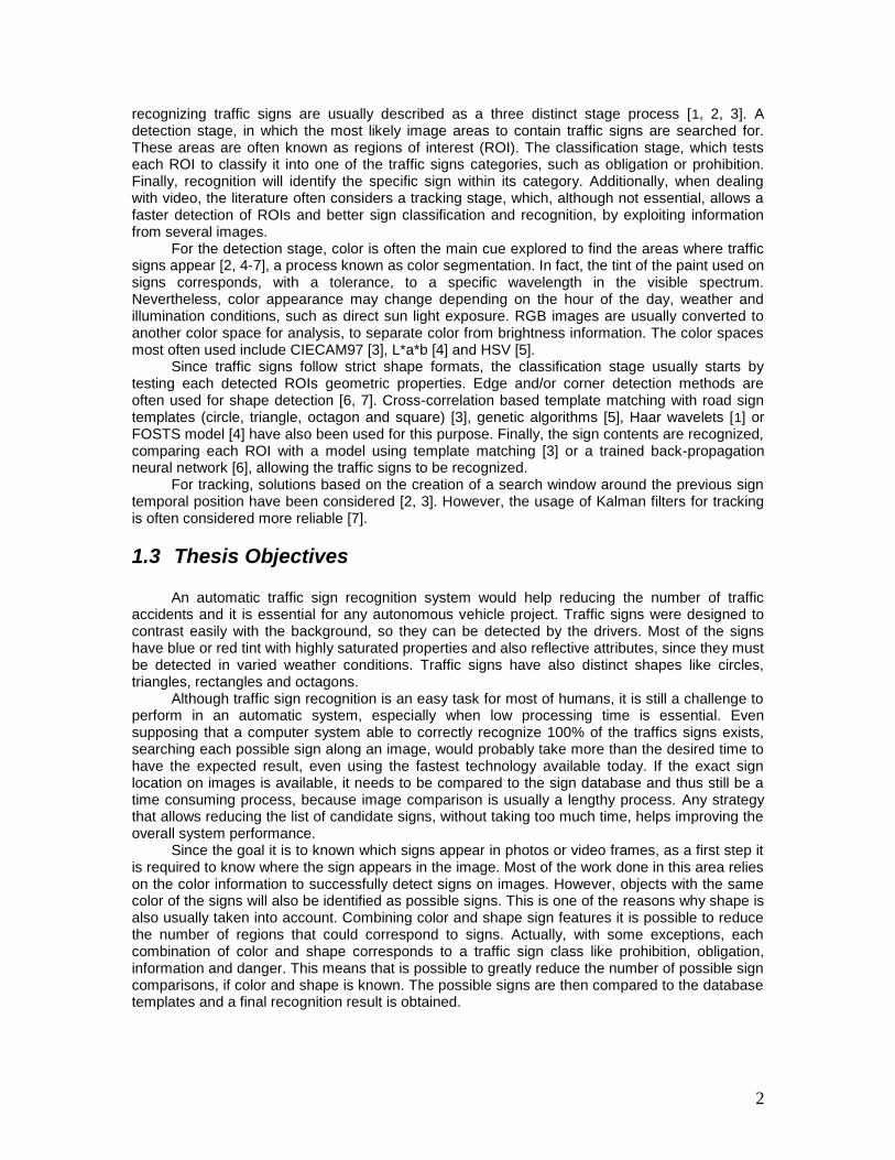
recognizing traffic signs are usually described as a three distinct stage process [1, 2, 3]. A detection stage, in which the most likely image areas to contain traffic signs are searched for. These areas are often known as regions of interest (ROI). The classification stage, which tests each ROI to classify it into one of the traffic signs categories, such as obligation or prohibition. Finally, recognition will identify the specific sign within its category. Additionally, when dealing with video, the literature often considers a tracking stage, which, although not essential, allows a faster detection of ROIs and better sign classification and recognition, by exploiting information from several images.
For the detection stage, color is often the main cue explored to find the areas where traffic signs appear [2, 4-7], a process known as color segmentation. In fact, the tint of the paint used on signs corresponds, with a tolerance, to a specific wavelength in the visible spectrum. Nevertheless, color appearance may change depending on the hour of the day, weather and illumination conditions, such as direct sun light exposure. RGB images are usually converted to another color space for analysis, to separate color from brightness information. The color spaces most often used include CIECAM97 [3], L*a*b [4] and HSV [5].
Since traffic signs follow strict shape formats, the classification stage usually starts by testing each detected ROIs geometric properties. Edge and/or corner detection methods are often used for shape detection [6, 7]. Cross-correlation based template matching with road sign templates (circle, triangle, octagon and square) [3], genetic algorithms [5], Haar wavelets [1] or FOSTS model [4] have also been used for this purpose. Finally, the sign contents are recognized, comparing each ROI with a model using template matching [3] or a trained back-propagation neural network [6], allowing the traffic signs to be recognized.
For tracking, solutions based on the creation of a search window around the previous sign temporal position have been considered [2, 3]. However, the usage of Kalman filters for tracking is often considered more reliable [7].
1.3 Thesis Objectives An automatic traffic sign recognition system would help reducing the number of traffic
accidents and it is essential for any autonomous vehicle project. Traffic signs were designed to contrast easily with the background, so they can be detected by the drivers. Most of the signs have blue or red tint with highly saturated properties and also reflective attributes, since they must be detected in varied weather conditions. Traffic signs have also distinct shapes like circles, triangles, rectangles and octagons.
Although traffic sign recognition is an easy task for most of humans, it is still a challenge to perform in an automatic system, especially when low processing time is essential. Even supposing that a computer system able to correctly recognize 100% of the traffics signs exists, searching each possible sign along an image, would probably take more than the desired time to have the expected result, even using the fastest technology available today. If the exact sign location on images is available, it needs to be compared to the sign database and thus still be a time consuming process, because image comparison is usually a lengthy process. Any strategy that allows reducing the list of candidate signs, without taking too much time, helps improving the overall system performance.
Since the goal it is to known which signs appear in photos or video frames, as a first step it is required to know where the sign appears in the image. Most of the work done in this area relies on the color information to successfully detect signs on images. However, objects with the same color of the signs will also be identified as possible signs. This is one of the reasons why shape is also usually taken into account. Combining color and shape sign features it is possible to reduce the number of regions that could correspond to signs. Actually, with some exceptions, each combination of color and shape corresponds to a traffic sign class like prohibition, obligation, information and danger. This means that is possible to greatly reduce the number of possible sign comparisons, if color and shape is known. The possible signs are then compared to the database templates and a final recognition result is obtained.
3
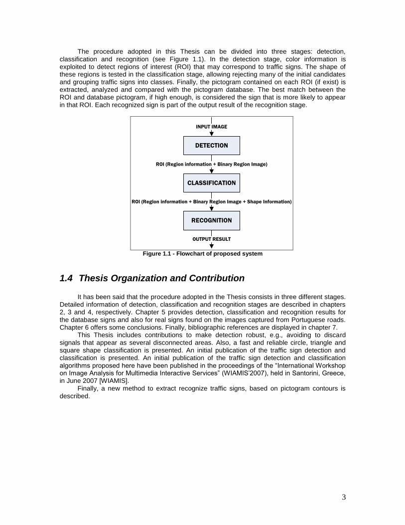
The procedure adopted in this Thesis can be divided into three stages: detection, classification and recognition (see Figure 1.1). In the detection stage, color information is exploited to detect regions of interest (ROI) that may correspond to traffic signs. The shape of these regions is tested in the classification stage, allowing rejecting many of the initial candidates and grouping traffic signs into classes. Finally, the pictogram contained on each ROI (if exist) is extracted, analyzed and compared with the pictogram database. The best match between the ROI and database pictogram, if high enough, is considered the sign that is more likely to appear in that ROI. Each recognized sign is part of the output result of the recognition stage.
DETECTION
CLASSIFICATION
ROI (Region information + Binary Region Image)
INPUT IMAGE
ROI (Region information + Binary Region Image + Shape Information)
RECOGNITION
OUTPUT RESULT
Figure 1.1 - Flowchart of proposed system
1.4 Thesis Organization and Contribution It has been said that the procedure adopted in the Thesis consists in three different stages.
Detailed information of detection, classification and recognition stages are described in chapters 2, 3 and 4, respectively. Chapter 5 provides detection, classification and recognition results for the database signs and also for real signs found on the images captured from Portuguese roads. Chapter 6 offers some conclusions. Finally, bibliographic references are displayed in chapter 7.
This Thesis includes contributions to make detection robust, e.g., avoiding to discard signals that appear as several disconnected areas. Also, a fast and reliable circle, triangle and square shape classification is presented. An initial publication of the traffic sign detection and classification is presented. An initial publication of the traffic sign detection and classification algorithms proposed here have been published in the proceedings of the “International Workshop on Image Analysis for Multimedia Interactive Services” (WIAMIS‟2007), held in Santorini, Greece, in June 2007 [WIAMIS].
Finally, a new method to extract recognize traffic signs, based on pictogram contours is described.
4
2 Detection
The detection of traffic signs, assumes a crucial role in any traffic sign recognition application. In fact, a sign that is not correctly detected cannot be classified and recognized to inform the driver. For instance, when the sign area is not completely detected, bad classification and recognition are likely to occur.
As stated in the introduction, color is explored for sign detection. Each input image is searched for areas that have colors similar to the ones present in traffic signs, resulting in a detection image where each pixel takes values between 0 (black) and 1 (white), where the highest values represent high color similarity. Blue and red colors are the ones to be detected, since, in this Thesis, the detection is tuned for Portuguese signs, where these two colors are the most used. To successfully identify the regions with color characteristics similar to those of traffic signs, the previous detection image is thresholded, resulting in a binarized image, composed by a number of regions (defined by 8-connected white pixels). Also, to easily identify each region found, a unique label number is associated to each one.
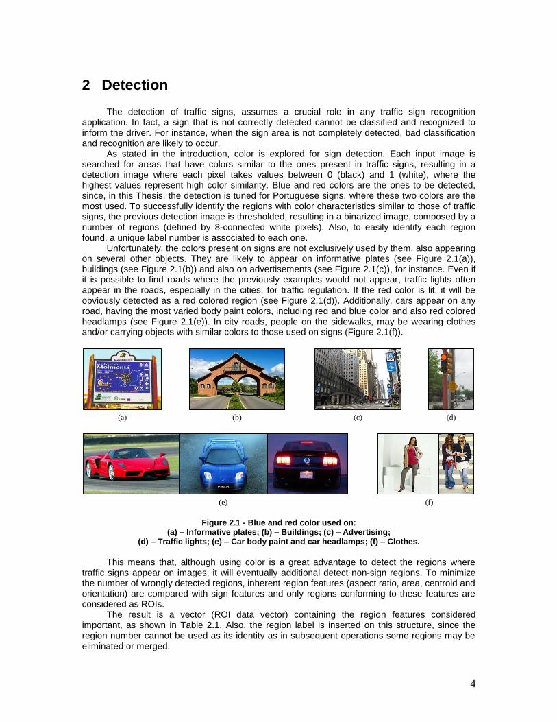
Unfortunately, the colors present on signs are not exclusively used by them, also appearing on several other objects. They are likely to appear on informative plates (see Figure 2.1(a)), buildings (see Figure 2.1(b)) and also on advertisements (see Figure 2.1(c)), for instance. Even if it is possible to find roads where the previously examples would not appear, traffic lights often appear in the roads, especially in the cities, for traffic regulation. If the red color is lit, it will be obviously detected as a red colored region (see Figure 2.1(d)). Additionally, cars appear on any road, having the most varied body paint colors, including red and blue color and also red colored headlamps (see Figure 2.1(e)). In city roads, people on the sidewalks, may be wearing clothes and/or carrying objects with similar colors to those used on signs (Figure 2.1(f)).
(a) (b) (c)
(e) (f)
(d)
Figure 2.1 - Blue and red color used on: (a) – Informative plates; (b) – Buildings; (c) – Advertising;
(d) – Traffic lights; (e) – Car body paint and car headlamps; (f) – Clothes. This means that, although using color is a great advantage to detect the regions where
traffic signs appear on images, it will eventually additional detect non-sign regions. To minimize the number of wrongly detected regions, inherent region features (aspect ratio, area, centroid and orientation) are compared with sign features and only regions conforming to these features are considered as ROIs.
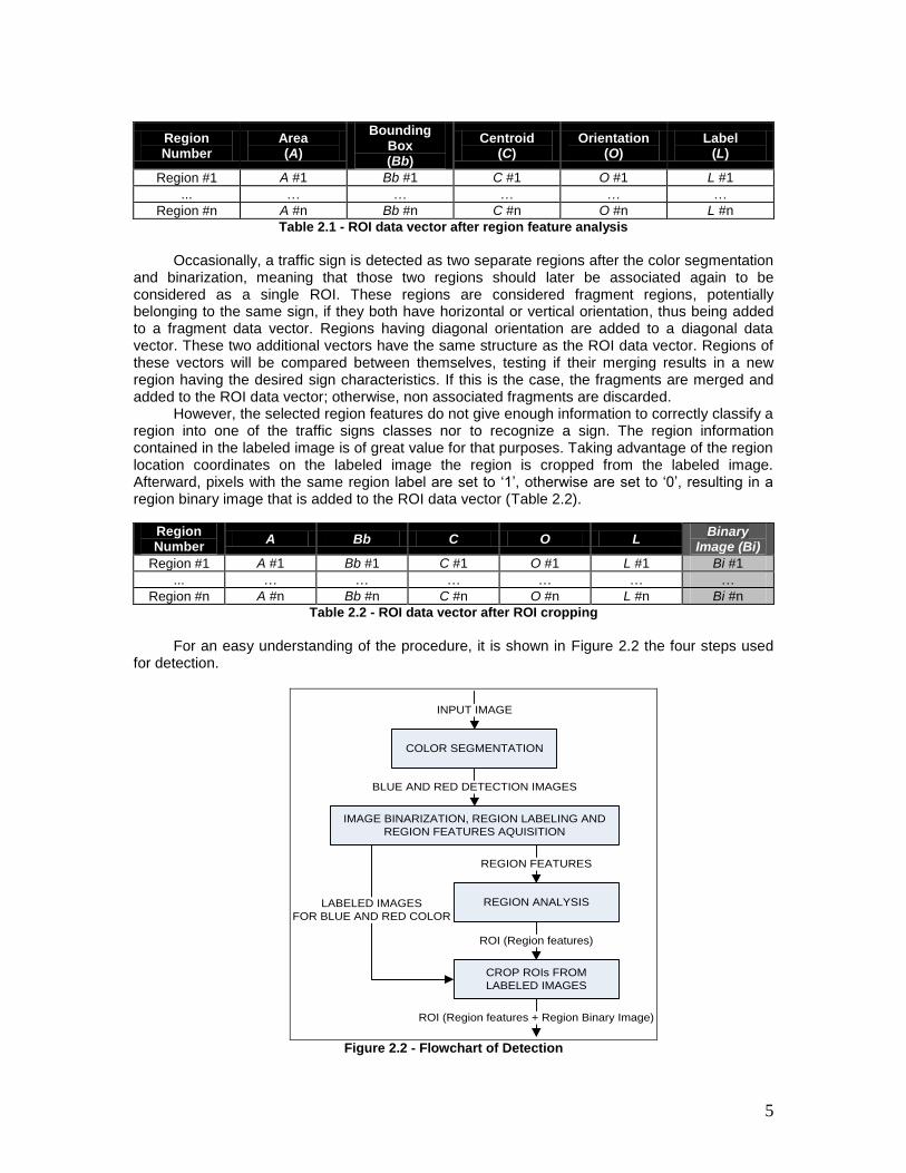
The result is a vector (ROI data vector) containing the region features considered important, as shown in Table 2.1. Also, the region label is inserted on this structure, since the region number cannot be used as its identity as in subsequent operations some regions may be eliminated or merged.
5
Region Number
Area (A)
Bounding Box (Bb)
Centroid (C)
Orientation (O)
Label (L)
Region #1 A #1 Bb #1 C #1 O #1 L #1
... … … … … …
Region #n A #n Bb #n C #n O #n L #n
Table 2.1 - ROI data vector after region feature analysis
Occasionally, a traffic sign is detected as two separate regions after the color segmentation
and binarization, meaning that those two regions should later be associated again to be considered as a single ROI. These regions are considered fragment regions, potentially belonging to the same sign, if they both have horizontal or vertical orientation, thus being added to a fragment data vector. Regions having diagonal orientation are added to a diagonal data vector. These two additional vectors have the same structure as the ROI data vector. Regions of these vectors will be compared between themselves, testing if their merging results in a new region having the desired sign characteristics. If this is the case, the fragments are merged and added to the ROI data vector; otherwise, non associated fragments are discarded.
However, the selected region features do not give enough information to correctly classify a region into one of the traffic signs classes nor to recognize a sign. The region information contained in the labeled image is of great value for that purposes. Taking advantage of the region location coordinates on the labeled image the region is cropped from the labeled image. Afterward, pixels with the same region label are set to „1‟, otherwise are set to „0‟, resulting in a region binary image that is added to the ROI data vector (Table 2.2).
Region Number
A Bb C O L Binary
Image (Bi)
Region #1 A #1 Bb #1 C #1 O #1 L #1 Bi #1
... … … … … … …
Region #n A #n Bb #n C #n O #n L #n Bi #n
Table 2.2 - ROI data vector after ROI cropping
For an easy understanding of the procedure, it is shown in Figure 2.2 the four steps used
for detection.
COLOR SEGMENTATION
IMAGE BINARIZATION, REGION LABELING AND
REGION FEATURES AQUISITION
BLUE AND RED DETECTION IMAGES
INPUT IMAGE
REGION FEATURES
REGION ANALYSIS
CROP ROIs FROM
LABELED IMAGES
ROI (Region features)
ROI (Region features + Region Binary Image)
LABELED IMAGES
FOR BLUE AND RED COLOR
Figure 2.2 - Flowchart of Detection
6
A more detailed explanation of each step will be made in the following subsections.
2.1 Color Segmentation The purpose of the color segmentation step is to separate the color of interest from the others
present in an image, allowing to locate signs on images by searching for their color. This could be a flawless detection method, knowing that sign colors are standardized for each country, however it is likely to find signs that don‟t have exactly the same original color and this difference tends to grow for older signs where the color has changed due to environmental conditions like sun exposure.
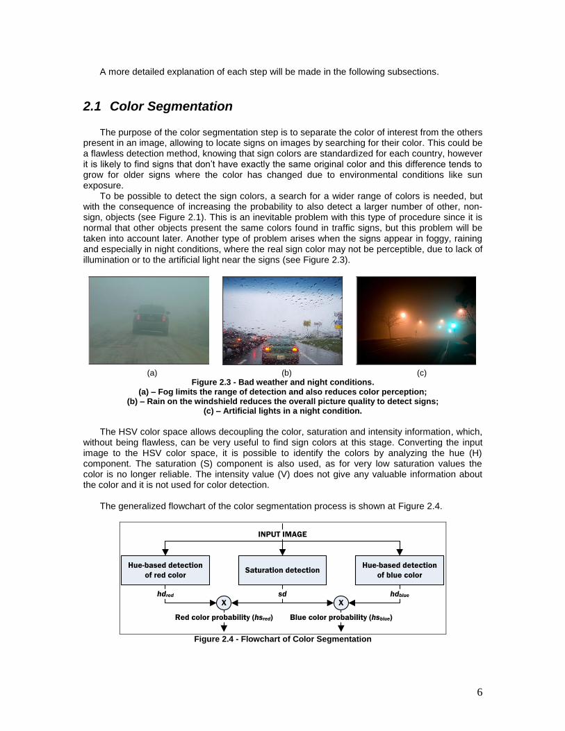
To be possible to detect the sign colors, a search for a wider range of colors is needed, but with the consequence of increasing the probability to also detect a larger number of other, non-sign, objects (see Figure 2.1). This is an inevitable problem with this type of procedure since it is normal that other objects present the same colors found in traffic signs, but this problem will be taken into account later. Another type of problem arises when the signs appear in foggy, raining and especially in night conditions, where the real sign color may not be perceptible, due to lack of illumination or to the artificial light near the signs (see Figure 2.3).
(a) (b) (c)
Figure 2.3 - Bad weather and night conditions. (a) – Fog limits the range of detection and also reduces color perception;
(b) – Rain on the windshield reduces the overall picture quality to detect signs; (c) – Artificial lights in a night condition.
The HSV color space allows decoupling the color, saturation and intensity information, which,
without being flawless, can be very useful to find sign colors at this stage. Converting the input image to the HSV color space, it is possible to identify the colors by analyzing the hue (H) component. The saturation (S) component is also used, as for very low saturation values the color is no longer reliable. The intensity value (V) does not give any valuable information about the color and it is not used for color detection.
The generalized flowchart of the color segmentation process is shown at Figure 2.4.
Hue-based detection
of red colorSaturation detection
Hue-based detection
of blue color
INPUT IMAGE
X Xhdred hdbluesd
Red color probability (hsred) Blue color probability (hsblue)
Figure 2.4 - Flowchart of Color Segmentation
7
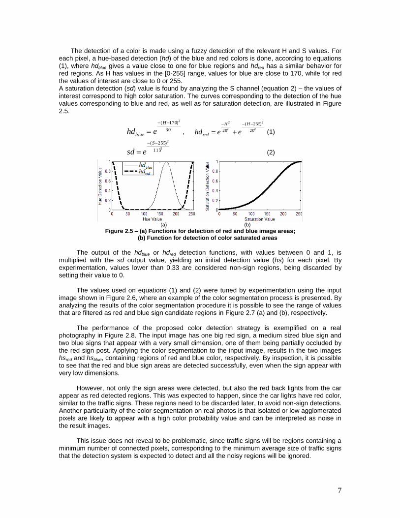
The detection of a color is made using a fuzzy detection of the relevant H and S values. For each pixel, a hue-based detection (hd) of the blue and red colors is done, according to equations (1), where hdblue gives a value close to one for blue regions and hdred has a similar behavior for red regions. As H has values in the [0-255] range, values for blue are close to 170, while for red the values of interest are close to 0 or 255. A saturation detection (sd) value is found by analyzing the S channel (equation 2) – the values of interest correspond to high color saturation. The curves corresponding to the detection of the hue values corresponding to blue and red, as well as for saturation detection, are illustrated in Figure 2.5.
30
)170( 2
H
blue ehd , 2
2
2
2
20
)255(
20
HH
red eehd (1)
2
2
115
)255(
S
esd (2)
(a) (b)
Figure 2.5 – (a) Functions for detection of red and blue image areas; (b) Function for detection of color saturated areas
The output of the hdblue or hdred detection functions, with values between 0 and 1, is
multiplied with the sd output value, yielding an initial detection value (hs) for each pixel. By experimentation, values lower than 0.33 are considered non-sign regions, being discarded by setting their value to 0.
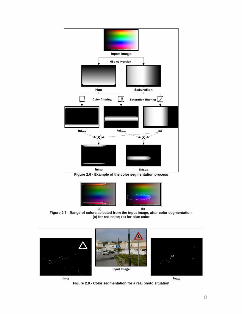
The values used on equations (1) and (2) were tuned by experimentation using the input
image shown in Figure 2.6, where an example of the color segmentation process is presented. By analyzing the results of the color segmentation procedure it is possible to see the range of values that are filtered as red and blue sign candidate regions in Figure 2.7 (a) and (b), respectively.
The performance of the proposed color detection strategy is exemplified on a real
photography in Figure 2.8. The input image has one big red sign, a medium sized blue sign and two blue signs that appear with a very small dimension, one of them being partially occluded by the red sign post. Applying the color segmentation to the input image, results in the two images hsred and hsblue, containing regions of red and blue color, respectively. By inspection, it is possible to see that the red and blue sign areas are detected successfully, even when the sign appear with very low dimensions.
However, not only the sign areas were detected, but also the red back lights from the car
appear as red detected regions. This was expected to happen, since the car lights have red color, similar to the traffic signs. These regions need to be discarded later, to avoid non-sign detections. Another particularity of the color segmentation on real photos is that isolated or low agglomerated pixels are likely to appear with a high color probability value and can be interpreted as noise in the result images.
This issue does not reveal to be problematic, since traffic signs will be regions containing a
minimum number of connected pixels, corresponding to the minimum average size of traffic signs that the detection system is expected to detect and all the noisy regions will be ignored.
8
Color filtering Saturation filtering
HSV conversion
Input Image
Saturation
hdred hdblue sd
X X
Hue
hsbluehsred Figure 2.6 - Example of the color segmentation process
(a) (b)
Figure 2.7 - Range of colors selected from the input image, after color segmentation, (a) for red color; (b) for blue color
Input Image
hsred hsblue Figure 2.8 - Color segmentation for a real photo situation
9
The color segmentation previously presented works very well for a large variety of images with good color definition. However, the color of signs with high brightness is not always detected and a lot of dark areas were often misclassified as a being of sign color. Having said that and looking at Figure 2.7, probably the color tolerance initially considered was not ideal. The dark color pixels should not be detected, since they don‟t have enough color information to allow a confident decision about their color and probably increasing the tolerance for handling brighter images would permit detection of the previously missed detections.
Instead of taking advantage of a typical HSV conversion, a new conversion based on the
HSV has been adopted, as described in the following. To distinguish the method that will be further presented, from the previous one, they will be referred as method #2 and method #1, respectively. For an input image in RGB format, the initial conversion to HSV is done according to equations (3), (4) and (5), where MAX and MIN are equal to the maximum and minimum of (R, G, B) pixel values, respectively.
,24060
,12060
)()( ,36060
)()( ,60
,
BMAXMINMAX
GR
GMAXMINMAX
RB
BGRMAXMINMAX
BG
BGRMAXMINMAX
BG
MINMAXundefined
H (3)
otherwiseMAX
MAXS
,1
0,0 (4)
MAXV (5)
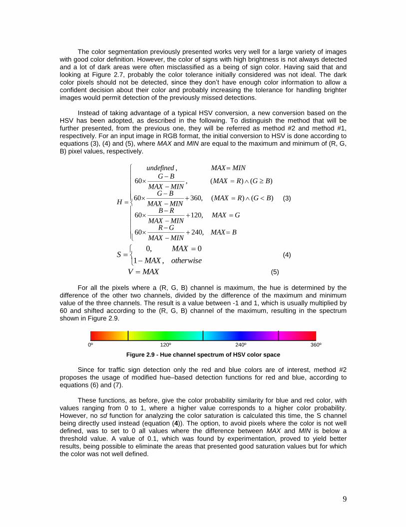
For all the pixels where a (R, G, B) channel is maximum, the hue is determined by the
difference of the other two channels, divided by the difference of the maximum and minimum value of the three channels. The result is a value between -1 and 1, which is usually multiplied by 60 and shifted according to the (R, G, B) channel of the maximum, resulting in the spectrum shown in Figure 2.9.
0º 240º120º 360º
Figure 2.9 - Hue channel spectrum of HSV color space
Since for traffic sign detection only the red and blue colors are of interest, method #2
proposes the usage of modified hue–based detection functions for red and blue, according to equations (6) and (7).
These functions, as before, give the color probability similarity for blue and red color, with
values ranging from 0 to 1, where a higher value corresponds to a higher color probability. However, no sd function for analyzing the color saturation is calculated this time, the S channel being directly used instead (equation (4)). The option, to avoid pixels where the color is not well defined, was to set to 0 all values where the difference between MAX and MIN is below a threshold value. A value of 0.1, which was found by experimentation, proved to yield better results, being possible to eliminate the areas that presented good saturation values but for which the color was not well defined.
10
otherwise
thMINMAXBMAXMINMAX
GR
hdblue
,0
)()(,
1 (6)
otherwise
thMINMAXRMAX,MINMAX
BG
hdred
,0
)()(1 (7)
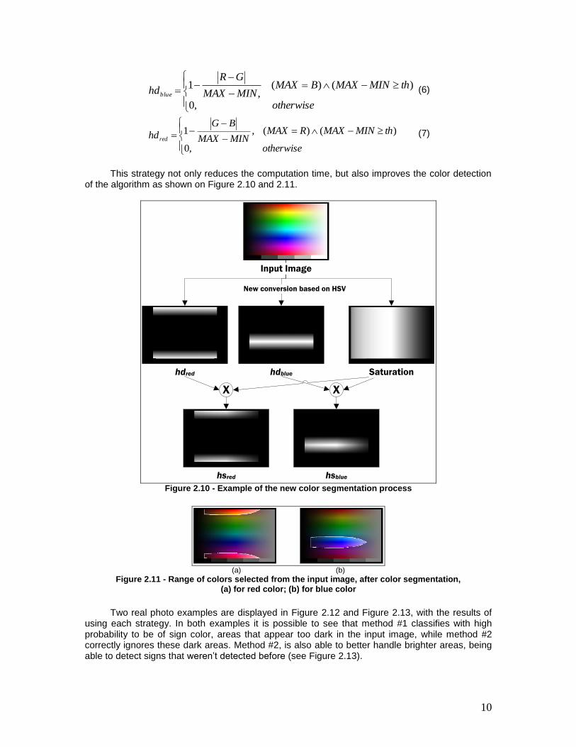
This strategy not only reduces the computation time, but also improves the color detection
of the algorithm as shown on Figure 2.10 and 2.11.
New conversion based on HSV
Input Image
Saturation
X X
hdred hdblue
hsred hsblue Figure 2.10 - Example of the new color segmentation process
(a) (b)
Figure 2.11 - Range of colors selected from the input image, after color segmentation, (a) for red color; (b) for blue color
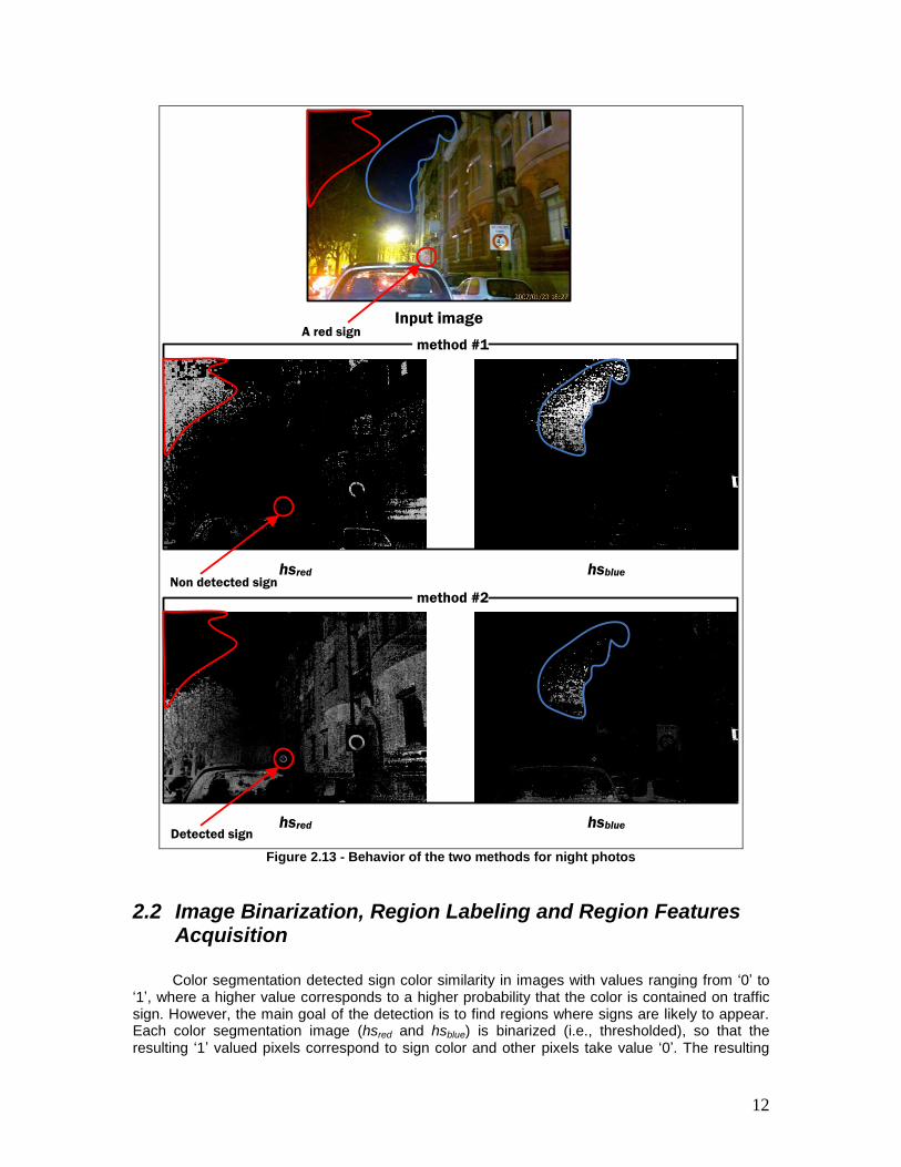
Two real photo examples are displayed in Figure 2.12 and Figure 2.13, with the results of
using each strategy. In both examples it is possible to see that method #1 classifies with high probability to be of sign color, areas that appear too dark in the input image, while method #2 correctly ignores these dark areas. Method #2, is also able to better handle brighter areas, being able to detect signs that weren‟t detected before (see Figure 2.13).
11
In a first impression, it may look that for the night photo example (Figure 2.13), method #1 results are better than method #2 results, since the last one classifies too much regions as red color, when it doesn‟t look that red in the image even if the building has a reddish color. The truth is that night photos usually have low color information and the RGB colors captured by a camera are less precise than for well illuminated photos. Also, the artificial illumination tends to change the color of surroundings and may change the sign color appearance, thus reducing the sign detection.
Nevertheless, it is preferable to detect more non-sign regions, than to miss sign detections,
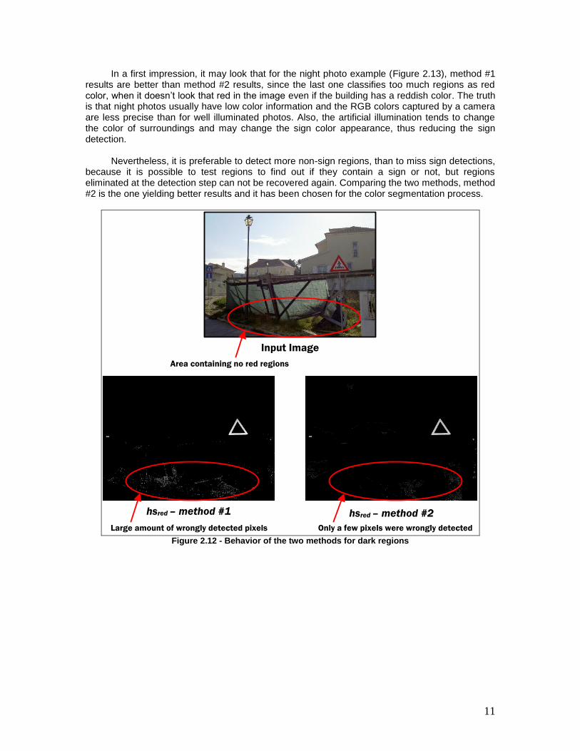
because it is possible to test regions to find out if they contain a sign or not, but regions eliminated at the detection step can not be recovered again. Comparing the two methods, method #2 is the one yielding better results and it has been chosen for the color segmentation process.
hsred – method #2hsred – method #1
Input Image
Area containing no red regions
Large amount of wrongly detected pixels Only a few pixels were wrongly detected Figure 2.12 - Behavior of the two methods for dark regions
12
Input image
hsbluehsred
hsred hsblue
method #2
method #1 A red sign
Non detected sign
Detected sign
Figure 2.13 - Behavior of the two methods for night photos
2.2 Image Binarization, Region Labeling and Region Features Acquisition
Color segmentation detected sign color similarity in images with values ranging from „0‟ to
„1‟, where a higher value corresponds to a higher probability that the color is contained on traffic sign. However, the main goal of the detection is to find regions where signs are likely to appear. Each color segmentation image (hsred and hsblue) is binarized (i.e., thresholded), so that the resulting „1‟ valued pixels correspond to sign color and other pixels take value „0‟. The resulting
13
binary image usually contains more than one detected region, where a region is considered to be any group of 8-connected „1‟ valued pixels. To easily identify each region a label is attributed to each one, resulting in a labeled image. Finally, a set of important region features is acquired for further processing.
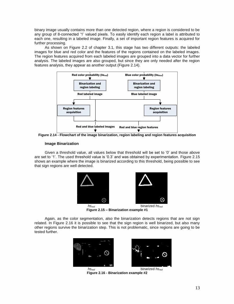
As shown on Figure 2.2 of chapter 3.1, this stage has two different outputs: the labeled images for blue and red color and the features of the regions contained on the labeled images. The region features acquired from each labeled images are grouped into a data vector for further analysis. The labeled images are also grouped, but since they are only needed after the region features analysis, they appear as another output (Figure 2.14).
Binarization and
region labeling
Binarization and
region labeling
Red color probability (hsred) Blue color probability (hsblue)
Red labeled image Blue labeled image
Red and blue labeled images
Region features
acquisition
Region features
acquisition
Red and blue region features
Figure 2.14 - Flowchart of the image binarization, region labeling and region features acquisition
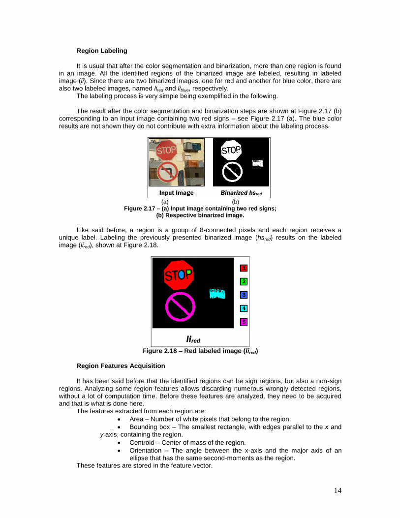
Image Binarization Given a threshold value, all values below that threshold will be set to „0‟ and those above
are set to „1‟. The used threshold value is „0.3‟ and was obtained by experimentation. Figure 2.15 shows an example where the image is binarized according to this threshold, being possible to see that sign regions are well detected.
hsred binarized hsred
Figure 2.15 – Binarization example #1
Again, as the color segmentation, also the binarization detects regions that are not sign
related. In Figure 2.16 it is possible to see that the sign region is well binarized, but also many other regions survive the binarization step. This is not problematic, since regions are going to be tested further.
hsred binarized hsred
Figure 2.16 - Binarization example #2
14
Region Labeling It is usual that after the color segmentation and binarization, more than one region is found
in an image. All the identified regions of the binarized image are labeled, resulting in labeled image (li). Since there are two binarized images, one for red and another for blue color, there are also two labeled images, named lired and liblue, respectively.
The labeling process is very simple being exemplified in the following. The result after the color segmentation and binarization steps are shown at Figure 2.17 (b)
corresponding to an input image containing two red signs – see Figure 2.17 (a). The blue color results are not shown they do not contribute with extra information about the labeling process.
Binarized hsredInput Image (a) (b)
Figure 2.17 – (a) Input image containing two red signs; (b) Respective binarized image.
Like said before, a region is a group of 8-connected pixels and each region receives a
unique label. Labeling the previously presented binarized image (hsred) results on the labeled image (lired), shown at Figure 2.18.
lired
1
2
5
4
3
Figure 2.18 – Red labeled image (lired)
Region Features Acquisition It has been said before that the identified regions can be sign regions, but also a non-sign
regions. Analyzing some region features allows discarding numerous wrongly detected regions, without a lot of computation time. Before these features are analyzed, they need to be acquired and that is what is done here.
The features extracted from each region are:
Area – Number of white pixels that belong to the region.
Bounding box – The smallest rectangle, with edges parallel to the x and y axis, containing the region.
Centroid – Center of mass of the region.
Orientation – The angle between the x-axis and the major axis of an ellipse that has the same second-moments as the region.
These features are stored in the feature vector.
15
2.3 Region Analysis
The regions detected after the color segmentation and binarization exhibit a color very
similar to the one expected to be found on traffic signs. However, the sign color may appear on other objects and so, those objects would be detected too.
In this step, the detected regions are tested for sign features including the region area, aspect ratio, respective centroid and orientation. Only regions with features conforming to the ones expected to be found on traffic signs will be considered as ROI.
The region area is useful to discard regions that appear too small, or too big, knowing that
there are expected sign sizes. Another factor that can be taken into account is that there is a minimum and maximum area percentage of the region bounding box, which must have the desired color to characterize that region as a sign. If a region is below this minimum or above the maximum, it is rejected as a ROI. The relation between the region area and the bounding box area is named as the region fulfillment (Rf).
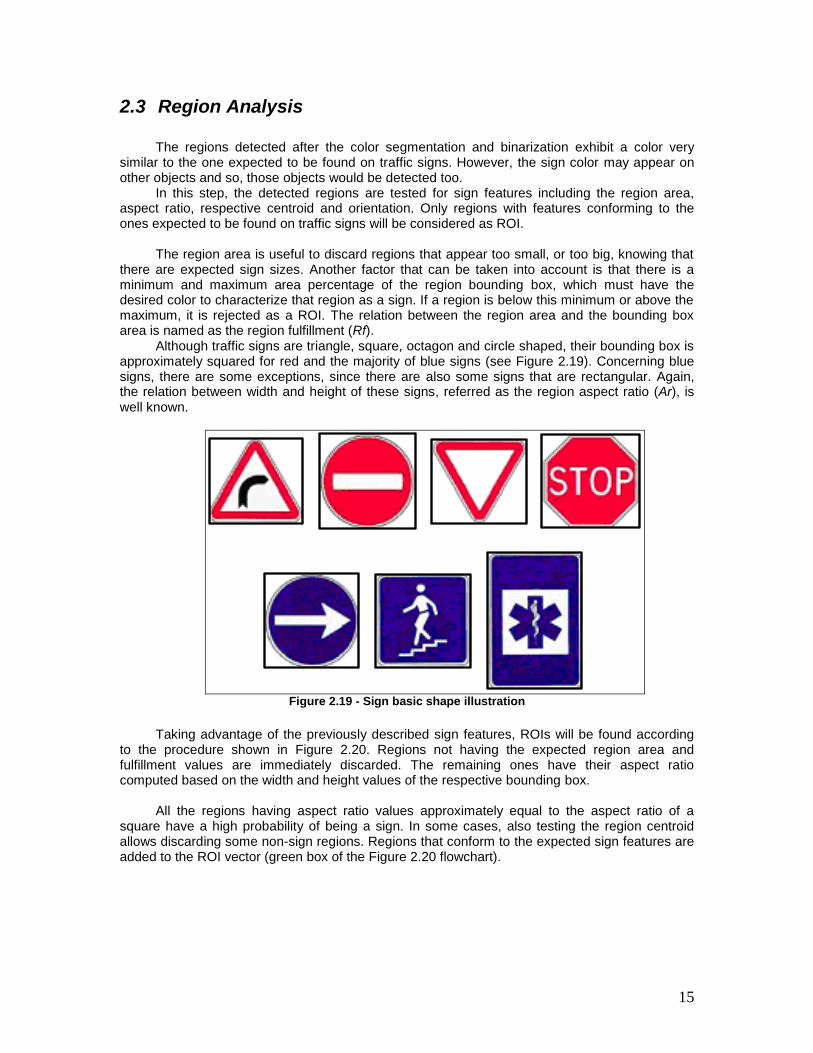
Although traffic signs are triangle, square, octagon and circle shaped, their bounding box is approximately squared for red and the majority of blue signs (see Figure 2.19). Concerning blue signs, there are some exceptions, since there are also some signs that are rectangular. Again, the relation between width and height of these signs, referred as the region aspect ratio (Ar), is well known.
Figure 2.19 - Sign basic shape illustration
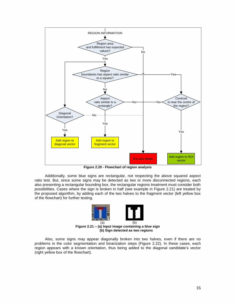
Taking advantage of the previously described sign features, ROIs will be found according
to the procedure shown in Figure 2.20. Regions not having the expected region area and fulfillment values are immediately discarded. The remaining ones have their aspect ratio computed based on the width and height values of the respective bounding box.
All the regions having aspect ratio values approximately equal to the aspect ratio of a
square have a high probability of being a sign. In some cases, also testing the region centroid allows discarding some non-sign regions. Regions that conform to the expected sign features are added to the ROI vector (green box of the Figure 2.20 flowchart).
16
REGION INFORMATION
Region area
and fulfillment has expected
values?
Discard shape
No
Region
boundaries has aspect ratio similar
to a square?
Yes
Add region to ROI
vector
Yes
Centroid
is near the centre of
the region?
Yes
No
Aspect
ratio similar to a
rectangle?
No
Add region to
fragment vector
Yes
Diagonal
Orientation?
Add region to
diagonal vector
Yes
No
No
Figure 2.20 - Flowchart of region analysis
Additionally, some blue signs are rectangular, not respecting the above squared aspect
ratio test. But, since some signs may be detected as two or more disconnected regions, each also presenting a rectangular bounding box, the rectangular regions treatment must consider both possibilities. Cases where the sign is broken in half (see example in Figure 2.21) are treated by the proposed algorithm, by adding each of the two halves to the fragment vector (left yellow box of the flowchart) for further testing.
(a) (b)
Figure 2.21 – (a) Input image containing a blue sign (b) Sign detected as two regions
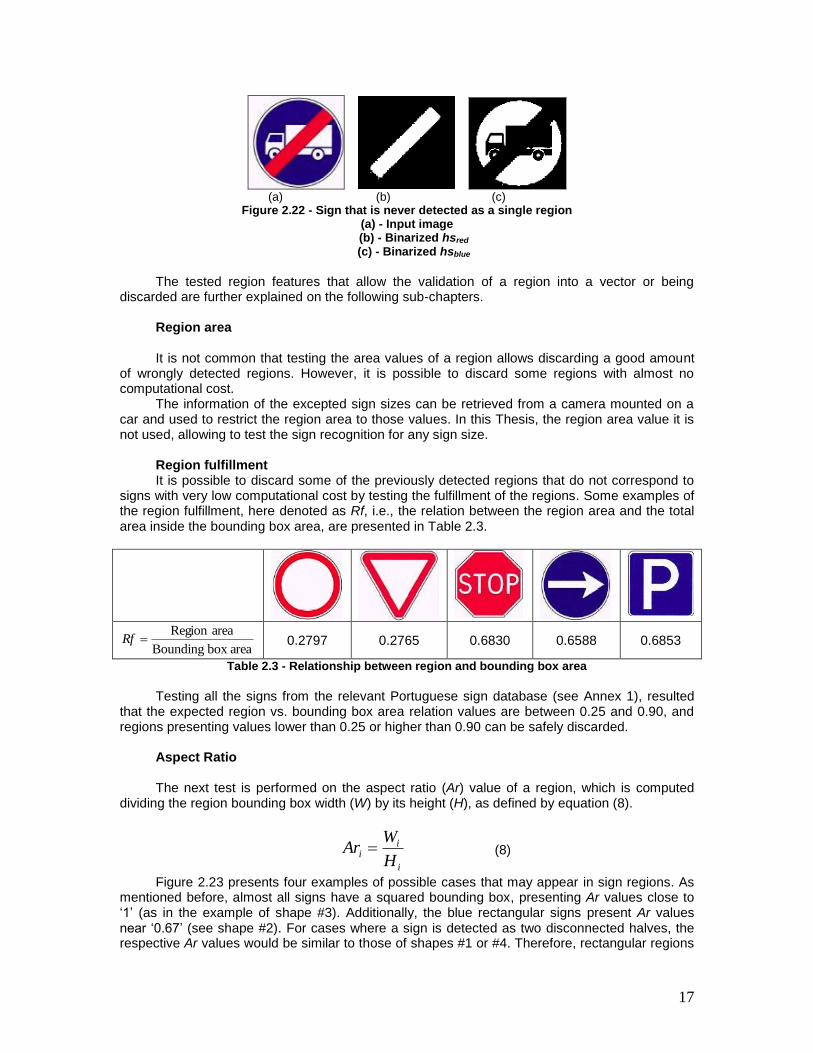
Also, some signs may appear diagonally broken into two halves, even if there are no
problems in the color segmentation and binarization steps (Figure 2.22). In these cases, each region appears with a known orientation, thus being added to the diagonal candidate‟s vector (right yellow box of the flowchart).
17
(a) (b) (c)
Figure 2.22 - Sign that is never detected as a single region (a) - Input image
(b) - Binarized hsred (c) - Binarized hsblue
The tested region features that allow the validation of a region into a vector or being
discarded are further explained on the following sub-chapters. Region area It is not common that testing the area values of a region allows discarding a good amount
of wrongly detected regions. However, it is possible to discard some regions with almost no computational cost.
The information of the excepted sign sizes can be retrieved from a camera mounted on a car and used to restrict the region area to those values. In this Thesis, the region area value it is not used, allowing to test the sign recognition for any sign size.
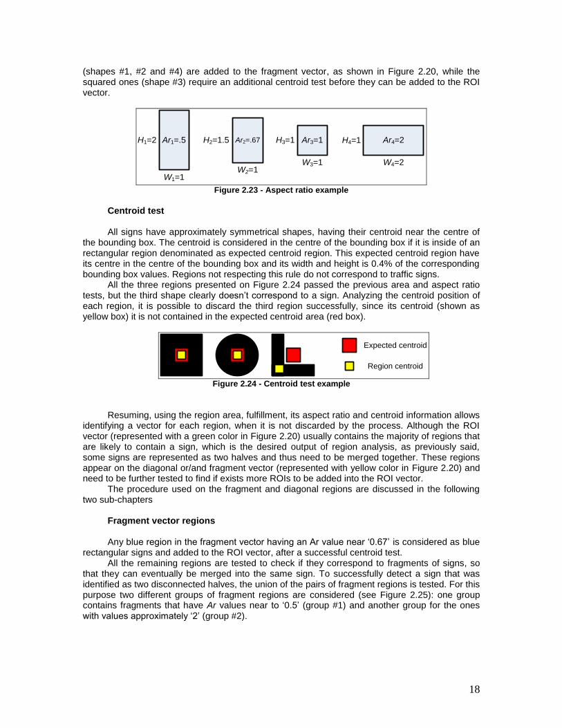
Region fulfillment It is possible to discard some of the previously detected regions that do not correspond to
signs with very low computational cost by testing the fulfillment of the regions. Some examples of the region fulfillment, here denoted as Rf, i.e., the relation between the region area and the total area inside the bounding box area, are presented in Table 2.3.
areabox Bounding
areaRegion Rf 0.2797 0.2765 0.6830 0.6588 0.6853
Table 2.3 - Relationship between region and bounding box area
Testing all the signs from the relevant Portuguese sign database (see Annex 1), resulted
that the expected region vs. bounding box area relation values are between 0.25 and 0.90, and regions presenting values lower than 0.25 or higher than 0.90 can be safely discarded.
Aspect Ratio The next test is performed on the aspect ratio (Ar) value of a region, which is computed
dividing the region bounding box width (W) by its height (H), as defined by equation (8).
i
ii
H
WAr (8)
Figure 2.23 presents four examples of possible cases that may appear in sign regions. As mentioned before, almost all signs have a squared bounding box, presenting Ar values close to „1‟ (as in the example of shape #3). Additionally, the blue rectangular signs present Ar values near „0.67‟ (see shape #2). For cases where a sign is detected as two disconnected halves, the respective Ar values would be similar to those of shapes #1 or #4. Therefore, rectangular regions
18
(shapes #1, #2 and #4) are added to the fragment vector, as shown in Figure 2.20, while the squared ones (shape #3) require an additional centroid test before they can be added to the ROI vector.
Ar1=.5 Ar3=1 Ar4=2
W1=1
W3=1 W4=2
H1=2 H3=1 H4=1Ar2=.67
W2=1
H2=1.5
Figure 2.23 - Aspect ratio example
Centroid test All signs have approximately symmetrical shapes, having their centroid near the centre of
the bounding box. The centroid is considered in the centre of the bounding box if it is inside of an rectangular region denominated as expected centroid region. This expected centroid region have its centre in the centre of the bounding box and its width and height is 0.4% of the corresponding bounding box values. Regions not respecting this rule do not correspond to traffic signs.
All the three regions presented on Figure 2.24 passed the previous area and aspect ratio tests, but the third shape clearly doesn‟t correspond to a sign. Analyzing the centroid position of each region, it is possible to discard the third region successfully, since its centroid (shown as yellow box) it is not contained in the expected centroid area (red box).
Expected centroid
Region centroid
Figure 2.24 - Centroid test example
Resuming, using the region area, fulfillment, its aspect ratio and centroid information allows
identifying a vector for each region, when it is not discarded by the process. Although the ROI vector (represented with a green color in Figure 2.20) usually contains the majority of regions that are likely to contain a sign, which is the desired output of region analysis, as previously said, some signs are represented as two halves and thus need to be merged together. These regions appear on the diagonal or/and fragment vector (represented with yellow color in Figure 2.20) and need to be further tested to find if exists more ROIs to be added into the ROI vector.
The procedure used on the fragment and diagonal regions are discussed in the following two sub-chapters
Fragment vector regions Any blue region in the fragment vector having an Ar value near „0.67‟ is considered as blue
rectangular signs and added to the ROI vector, after a successful centroid test. All the remaining regions are tested to check if they correspond to fragments of signs, so
that they can eventually be merged into the same sign. To successfully detect a sign that was identified as two disconnected halves, the union of the pairs of fragment regions is tested. For this purpose two different groups of fragment regions are considered (see Figure 2.25): one group contains fragments that have Ar values near to „0.5‟ (group #1) and another group for the ones with values approximately „2‟ (group #2).
19
1 2 31 2
Group #1 Group #2
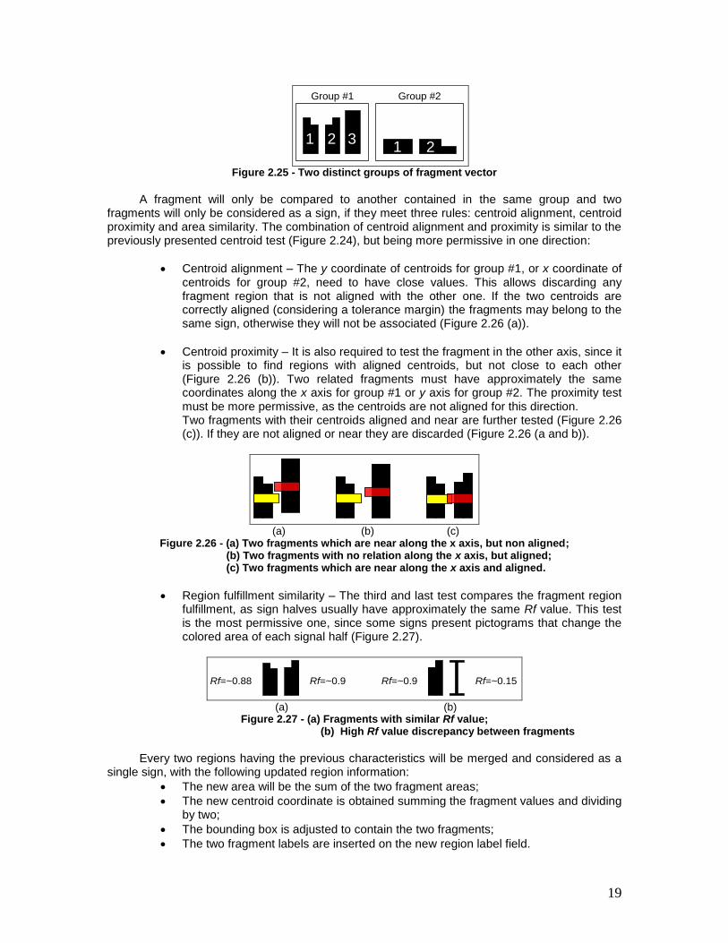
Figure 2.25 - Two distinct groups of fragment vector
A fragment will only be compared to another contained in the same group and two
fragments will only be considered as a sign, if they meet three rules: centroid alignment, centroid proximity and area similarity. The combination of centroid alignment and proximity is similar to the previously presented centroid test (Figure 2.24), but being more permissive in one direction:
Centroid alignment – The y coordinate of centroids for group #1, or x coordinate of centroids for group #2, need to have close values. This allows discarding any fragment region that is not aligned with the other one. If the two centroids are correctly aligned (considering a tolerance margin) the fragments may belong to the same sign, otherwise they will not be associated (Figure 2.26 (a)).
Centroid proximity – It is also required to test the fragment in the other axis, since it is possible to find regions with aligned centroids, but not close to each other (Figure 2.26 (b)). Two related fragments must have approximately the same coordinates along the x axis for group #1 or y axis for group #2. The proximity test must be more permissive, as the centroids are not aligned for this direction. Two fragments with their centroids aligned and near are further tested (Figure 2.26 (c)). If they are not aligned or near they are discarded (Figure 2.26 (a and b)).
(a) (b) (c)
Figure 2.26 - (a) Two fragments which are near along the x axis, but non aligned; (b) Two fragments with no relation along the x axis, but aligned;
(c) Two fragments which are near along the x axis and aligned.
Region fulfillment similarity – The third and last test compares the fragment region fulfillment, as sign halves usually have approximately the same Rf value. This test is the most permissive one, since some signs present pictograms that change the colored area of each signal half (Figure 2.27).
Rf=~0.88 Rf=~0.9 Rf=~0.9 Rf=~0.15
(a) (b)
Figure 2.27 - (a) Fragments with similar Rf value; (b) High Rf value discrepancy between fragments
Every two regions having the previous characteristics will be merged and considered as a
single sign, with the following updated region information:
The new area will be the sum of the two fragment areas;
The new centroid coordinate is obtained summing the fragment values and dividing by two;
The bounding box is adjusted to contain the two fragments;
The two fragment labels are inserted on the new region label field.
20
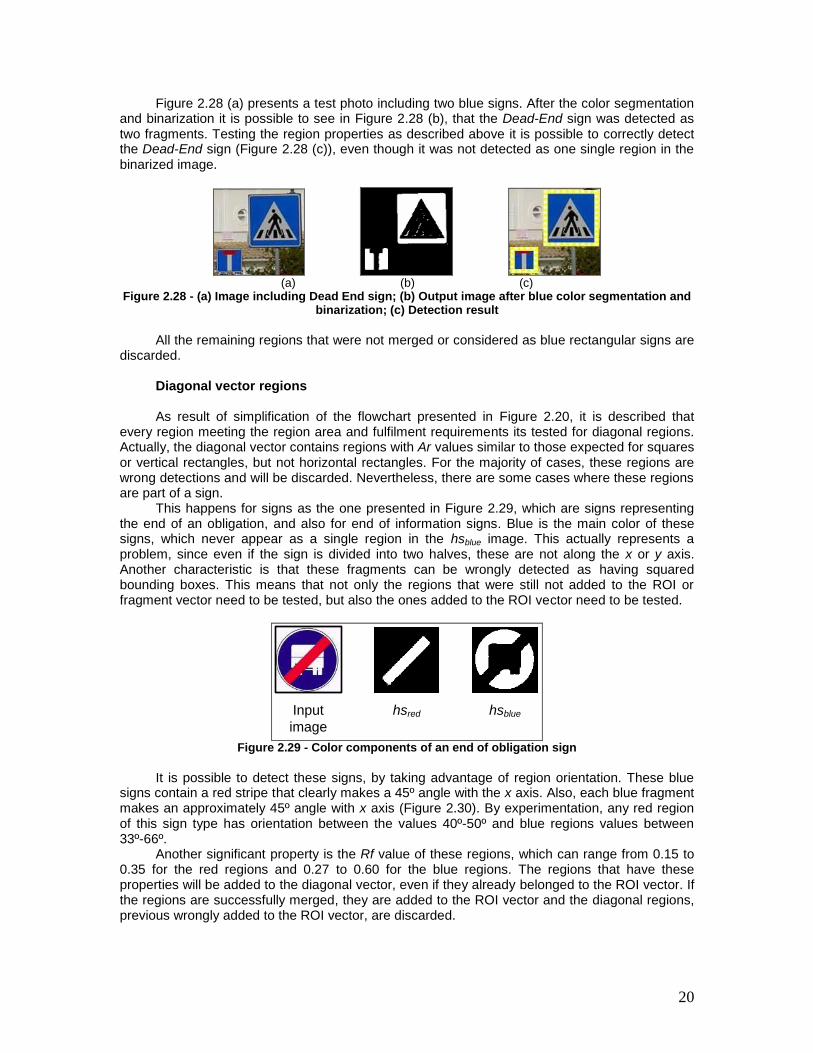
Figure 2.28 (a) presents a test photo including two blue signs. After the color segmentation and binarization it is possible to see in Figure 2.28 (b), that the Dead-End sign was detected as two fragments. Testing the region properties as described above it is possible to correctly detect the Dead-End sign (Figure 2.28 (c)), even though it was not detected as one single region in the binarized image.
(a) (b) (c)
Figure 2.28 - (a) Image including Dead End sign; (b) Output image after blue color segmentation and binarization; (c) Detection result
All the remaining regions that were not merged or considered as blue rectangular signs are
discarded.
Diagonal vector regions As result of simplification of the flowchart presented in Figure 2.20, it is described that
every region meeting the region area and fulfilment requirements its tested for diagonal regions. Actually, the diagonal vector contains regions with Ar values similar to those expected for squares or vertical rectangles, but not horizontal rectangles. For the majority of cases, these regions are wrong detections and will be discarded. Nevertheless, there are some cases where these regions are part of a sign.
This happens for signs as the one presented in Figure 2.29, which are signs representing the end of an obligation, and also for end of information signs. Blue is the main color of these signs, which never appear as a single region in the hsblue image. This actually represents a problem, since even if the sign is divided into two halves, these are not along the x or y axis. Another characteristic is that these fragments can be wrongly detected as having squared bounding boxes. This means that not only the regions that were still not added to the ROI or fragment vector need to be tested, but also the ones added to the ROI vector need to be tested.
Input
image
hsbluehsred
Figure 2.29 - Color components of an end of obligation sign
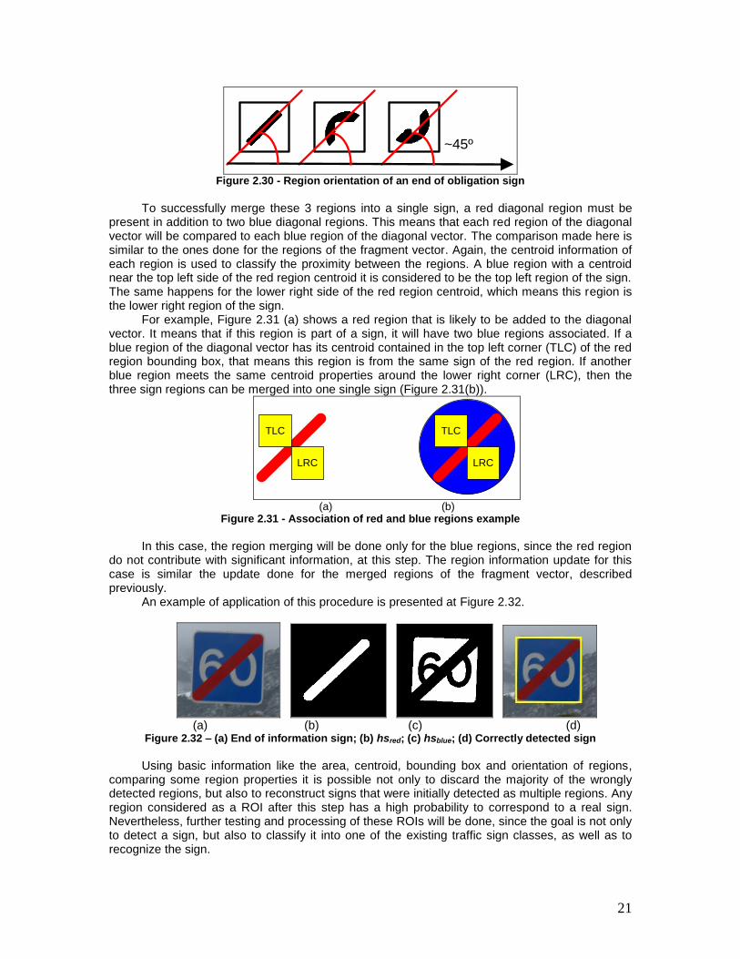
It is possible to detect these signs, by taking advantage of region orientation. These blue
signs contain a red stripe that clearly makes a 45º angle with the x axis. Also, each blue fragment makes an approximately 45º angle with x axis (Figure 2.30). By experimentation, any red region of this sign type has orientation between the values 40º-50º and blue regions values between 33º-66º.
Another significant property is the Rf value of these regions, which can range from 0.15 to 0.35 for the red regions and 0.27 to 0.60 for the blue regions. The regions that have these properties will be added to the diagonal vector, even if they already belonged to the ROI vector. If the regions are successfully merged, they are added to the ROI vector and the diagonal regions, previous wrongly added to the ROI vector, are discarded.
21
~45º
Figure 2.30 - Region orientation of an end of obligation sign
To successfully merge these 3 regions into a single sign, a red diagonal region must be
present in addition to two blue diagonal regions. This means that each red region of the diagonal vector will be compared to each blue region of the diagonal vector. The comparison made here is similar to the ones done for the regions of the fragment vector. Again, the centroid information of each region is used to classify the proximity between the regions. A blue region with a centroid near the top left side of the red region centroid it is considered to be the top left region of the sign. The same happens for the lower right side of the red region centroid, which means this region is the lower right region of the sign.
For example, Figure 2.31 (a) shows a red region that is likely to be added to the diagonal vector. It means that if this region is part of a sign, it will have two blue regions associated. If a blue region of the diagonal vector has its centroid contained in the top left corner (TLC) of the red region bounding box, that means this region is from the same sign of the red region. If another blue region meets the same centroid properties around the lower right corner (LRC), then the three sign regions can be merged into one single sign (Figure 2.31(b)).
TLC
LRC
TLC
LRC
(a) (b)
Figure 2.31 - Association of red and blue regions example
In this case, the region merging will be done only for the blue regions, since the red region
do not contribute with significant information, at this step. The region information update for this case is similar the update done for the merged regions of the fragment vector, described previously.
An example of application of this procedure is presented at Figure 2.32.
(a) (b) (c) (d)
Figure 2.32 – (a) End of information sign; (b) hsred; (c) hsblue; (d) Correctly detected sign
Using basic information like the area, centroid, bounding box and orientation of regions,
comparing some region properties it is possible not only to discard the majority of the wrongly detected regions, but also to reconstruct signs that were initially detected as multiple regions. Any region considered as a ROI after this step has a high probability to correspond to a real sign. Nevertheless, further testing and processing of these ROIs will be done, since the goal is not only to detect a sign, but also to classify it into one of the existing traffic sign classes, as well as to recognize the sign.
22
2.4 ROI Extraction
Even though some sign features were already taken into account, allowing to find regions
with high probability to contain a sign, there is still no indication as to the class to which the sign belongs, or a guarantee that it really is a traffic sign.
Here, sign classification is done by combining shape and color information, where the color is already known to be blue or red. The next step is check if the ROI shape is a triangle, square, octagon or a circle. Instead of doing shape classification by analysis of the full image and since ROIs were already identified, each one can be classified independently, providing more robustness and improving the classification performance.
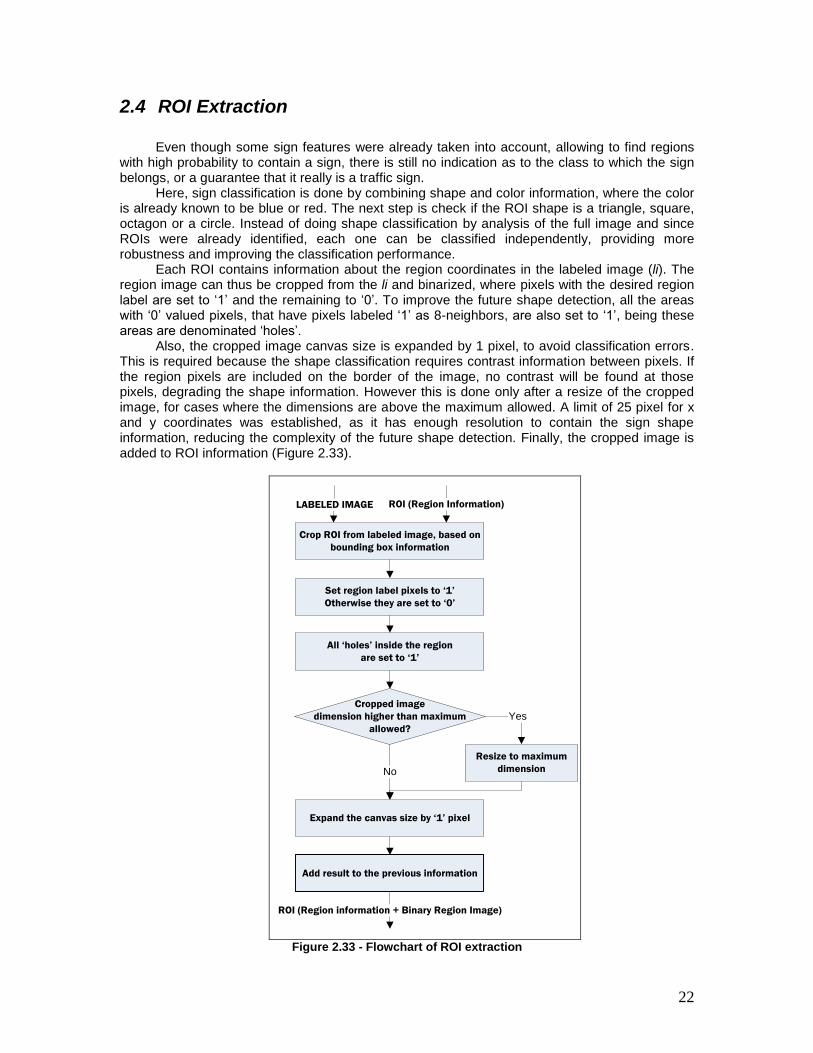
Each ROI contains information about the region coordinates in the labeled image (li). The region image can thus be cropped from the li and binarized, where pixels with the desired region label are set to „1‟ and the remaining to „0‟. To improve the future shape detection, all the areas with „0‟ valued pixels, that have pixels labeled „1‟ as 8-neighbors, are also set to „1‟, being these areas are denominated „holes‟.
Also, the cropped image canvas size is expanded by 1 pixel, to avoid classification errors. This is required because the shape classification requires contrast information between pixels. If the region pixels are included on the border of the image, no contrast will be found at those pixels, degrading the shape information. However this is done only after a resize of the cropped image, for cases where the dimensions are above the maximum allowed. A limit of 25 pixel for x and y coordinates was established, as it has enough resolution to contain the sign shape information, reducing the complexity of the future shape detection. Finally, the cropped image is added to ROI information (Figure 2.33).
Add result to the previous information
ROI (Region Information)
ROI (Region information + Binary Region Image)
LABELED IMAGE
Crop ROI from labeled image, based on
bounding box information
Set region label pixels to ‘1’
Otherwise they are set to ‘0’
All ‘holes’ inside the region
are set to ‘1’
Cropped image
dimension higher than maximum
allowed?
Resize to maximum
dimension
Yes
Expand the canvas size by ‘1’ pixel
No
Figure 2.33 - Flowchart of ROI extraction
23
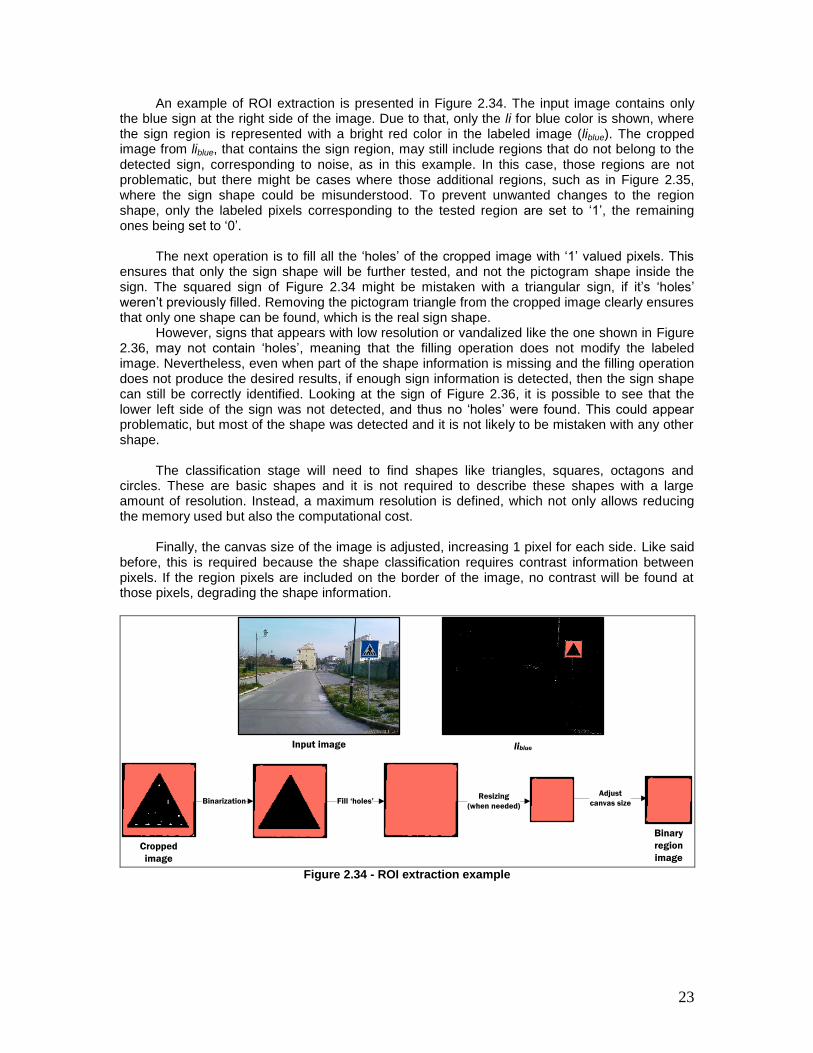
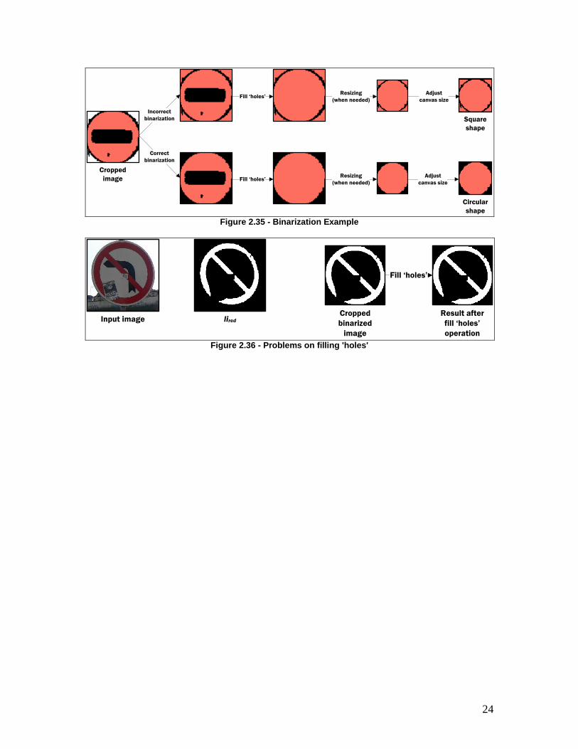
An example of ROI extraction is presented in Figure 2.34. The input image contains only the blue sign at the right side of the image. Due to that, only the li for blue color is shown, where the sign region is represented with a bright red color in the labeled image (liblue). The cropped image from liblue, that contains the sign region, may still include regions that do not belong to the detected sign, corresponding to noise, as in this example. In this case, those regions are not problematic, but there might be cases where those additional regions, such as in Figure 2.35, where the sign shape could be misunderstood. To prevent unwanted changes to the region shape, only the labeled pixels corresponding to the tested region are set to „1‟, the remaining ones being set to „0‟.
The next operation is to fill all the „holes‟ of the cropped image with „1‟ valued pixels. This
ensures that only the sign shape will be further tested, and not the pictogram shape inside the sign. The squared sign of Figure 2.34 might be mistaken with a triangular sign, if it‟s „holes‟ weren‟t previously filled. Removing the pictogram triangle from the cropped image clearly ensures that only one shape can be found, which is the real sign shape.
However, signs that appears with low resolution or vandalized like the one shown in Figure 2.36, may not contain „holes‟, meaning that the filling operation does not modify the labeled image. Nevertheless, even when part of the shape information is missing and the filling operation does not produce the desired results, if enough sign information is detected, then the sign shape can still be correctly identified. Looking at the sign of Figure 2.36, it is possible to see that the lower left side of the sign was not detected, and thus no „holes‟ were found. This could appear problematic, but most of the shape was detected and it is not likely to be mistaken with any other shape.
The classification stage will need to find shapes like triangles, squares, octagons and
circles. These are basic shapes and it is not required to describe these shapes with a large amount of resolution. Instead, a maximum resolution is defined, which not only allows reducing the memory used but also the computational cost.
Finally, the canvas size of the image is adjusted, increasing 1 pixel for each side. Like said
before, this is required because the shape classification requires contrast information between pixels. If the region pixels are included on the border of the image, no contrast will be found at those pixels, degrading the shape information.
Input image liblue
Cropped
image
Binarization Fill ‘holes’Resizing
(when needed)
Adjust
canvas size
Binary
region
image Figure 2.34 - ROI extraction example
24
Cropped
image
Incorrect
binarization
Fill ‘holes’Resizing
(when needed)
Square
shape
Adjust
canvas size
Correct
binarization
Fill ‘holes’Resizing
(when needed)
Circular
shape
Adjust
canvas size
Figure 2.35 - Binarization Example
Input image lired
Cropped
binarized
image
Result after
fill ‘holes’
operation
Fill ‘holes’
Figure 2.36 - Problems on filling 'holes'
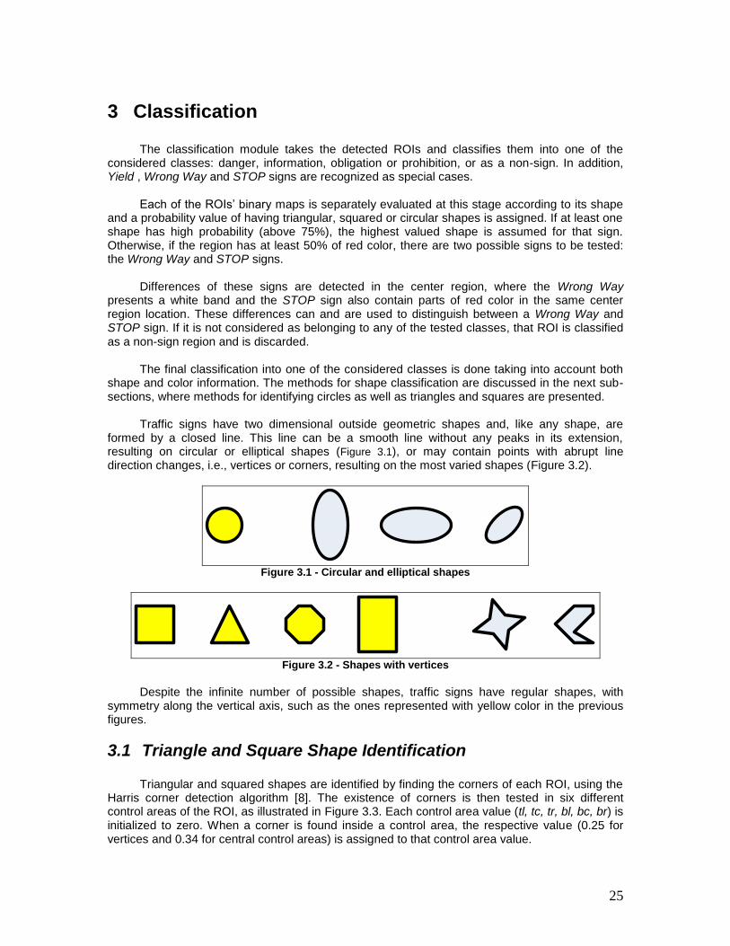
25
3 Classification
The classification module takes the detected ROIs and classifies them into one of the considered classes: danger, information, obligation or prohibition, or as a non-sign. In addition, Yield , Wrong Way and STOP signs are recognized as special cases.
Each of the ROIs‟ binary maps is separately evaluated at this stage according to its shape
and a probability value of having triangular, squared or circular shapes is assigned. If at least one shape has high probability (above 75%), the highest valued shape is assumed for that sign. Otherwise, if the region has at least 50% of red color, there are two possible signs to be tested: the Wrong Way and STOP signs.
Differences of these signs are detected in the center region, where the Wrong Way
presents a white band and the STOP sign also contain parts of red color in the same center region location. These differences can and are used to distinguish between a Wrong Way and STOP sign. If it is not considered as belonging to any of the tested classes, that ROI is classified as a non-sign region and is discarded.
The final classification into one of the considered classes is done taking into account both
shape and color information. The methods for shape classification are discussed in the next sub-sections, where methods for identifying circles as well as triangles and squares are presented.
Traffic signs have two dimensional outside geometric shapes and, like any shape, are
formed by a closed line. This line can be a smooth line without any peaks in its extension, resulting on circular or elliptical shapes (Figure 3.1), or may contain points with abrupt line direction changes, i.e., vertices or corners, resulting on the most varied shapes (Figure 3.2).
Figure 3.1 - Circular and elliptical shapes
Figure 3.2 - Shapes with vertices
Despite the infinite number of possible shapes, traffic signs have regular shapes, with
symmetry along the vertical axis, such as the ones represented with yellow color in the previous figures.
3.1 Triangle and Square Shape Identification
Triangular and squared shapes are identified by finding the corners of each ROI, using the Harris corner detection algorithm [8]. The existence of corners is then tested in six different control areas of the ROI, as illustrated in Figure 3.3. Each control area value (tl, tc, tr, bl, bc, br) is initialized to zero. When a corner is found inside a control area, the respective value (0.25 for vertices and 0.34 for central control areas) is assigned to that control area value.
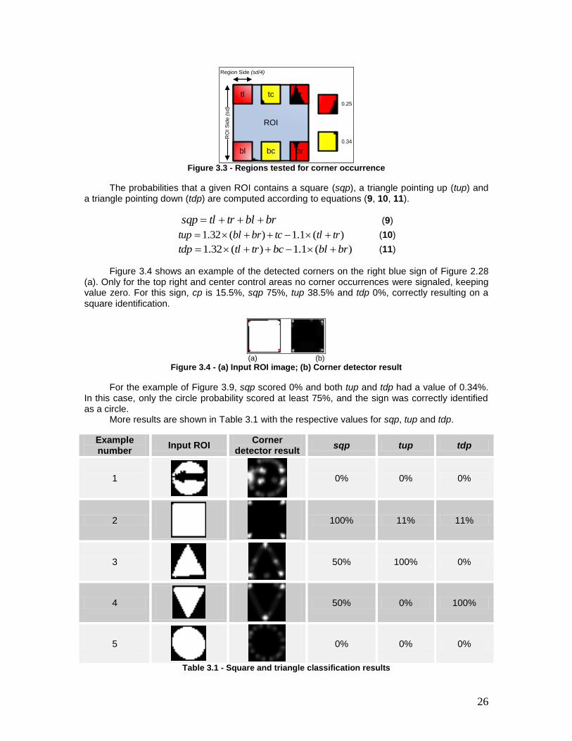
26
ROI
tl
bl
tr
brbc
tc0.25
0.34
RO
I S
ide
(sd
)
Region Side (sd/4)
Figure 3.3 - Regions tested for corner occurrence
The probabilities that a given ROI contains a square (sqp), a triangle pointing up (tup) and a triangle pointing down (tdp) are computed according to equations (9, 10, 11).
brbltrtlsqp (9)
)(1.1)(32.1 trtltcbrbltup (10)
)(1.1)(32.1 brblbctrtltdp (11)
Figure 3.4 shows an example of the detected corners on the right blue sign of Figure 2.28 (a). Only for the top right and center control areas no corner occurrences were signaled, keeping value zero. For this sign, cp is 15.5%, sqp 75%, tup 38.5% and tdp 0%, correctly resulting on a square identification.
(a) (b)
Figure 3.4 - (a) Input ROI image; (b) Corner detector result
For the example of Figure 3.9, sqp scored 0% and both tup and tdp had a value of 0.34%. In this case, only the circle probability scored at least 75%, and the sign was correctly identified as a circle.
More results are shown in Table 3.1 with the respective values for sqp, tup and tdp.
Example number
Input ROI Corner
detector result sqp tup tdp
1
0% 0% 0%
2
100% 11% 11%
3
50% 100% 0%
4
50% 0% 100%
5
0% 0% 0%
Table 3.1 - Square and triangle classification results
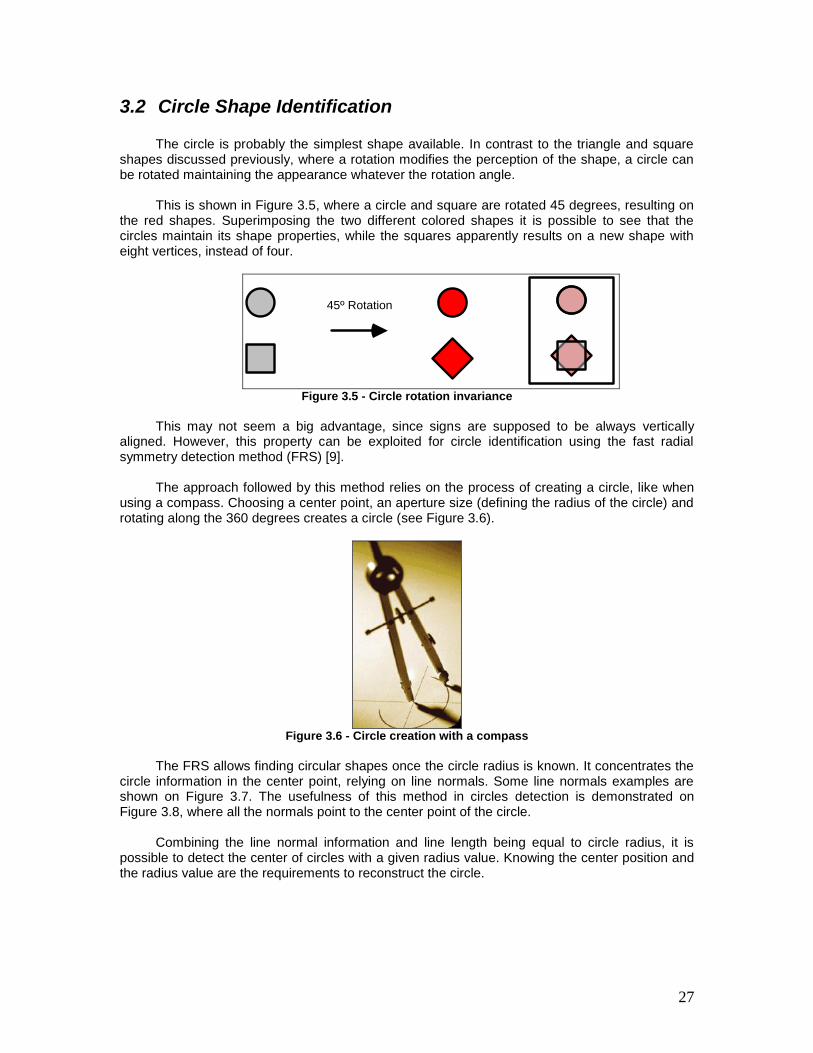
27
3.2 Circle Shape Identification
The circle is probably the simplest shape available. In contrast to the triangle and square shapes discussed previously, where a rotation modifies the perception of the shape, a circle can be rotated maintaining the appearance whatever the rotation angle.
This is shown in Figure 3.5, where a circle and square are rotated 45 degrees, resulting on
the red shapes. Superimposing the two different colored shapes it is possible to see that the circles maintain its shape properties, while the squares apparently results on a new shape with eight vertices, instead of four.
45º Rotation
Figure 3.5 - Circle rotation invariance
This may not seem a big advantage, since signs are supposed to be always vertically
aligned. However, this property can be exploited for circle identification using the fast radial symmetry detection method (FRS) [9].
The approach followed by this method relies on the process of creating a circle, like when
using a compass. Choosing a center point, an aperture size (defining the radius of the circle) and rotating along the 360 degrees creates a circle (see Figure 3.6).
Figure 3.6 - Circle creation with a compass
The FRS allows finding circular shapes once the circle radius is known. It concentrates the
circle information in the center point, relying on line normals. Some line normals examples are shown on Figure 3.7. The usefulness of this method in circles detection is demonstrated on Figure 3.8, where all the normals point to the center point of the circle.
Combining the line normal information and line length being equal to circle radius, it is
possible to detect the center of circles with a given radius value. Knowing the center position and the radius value are the requirements to reconstruct the circle.
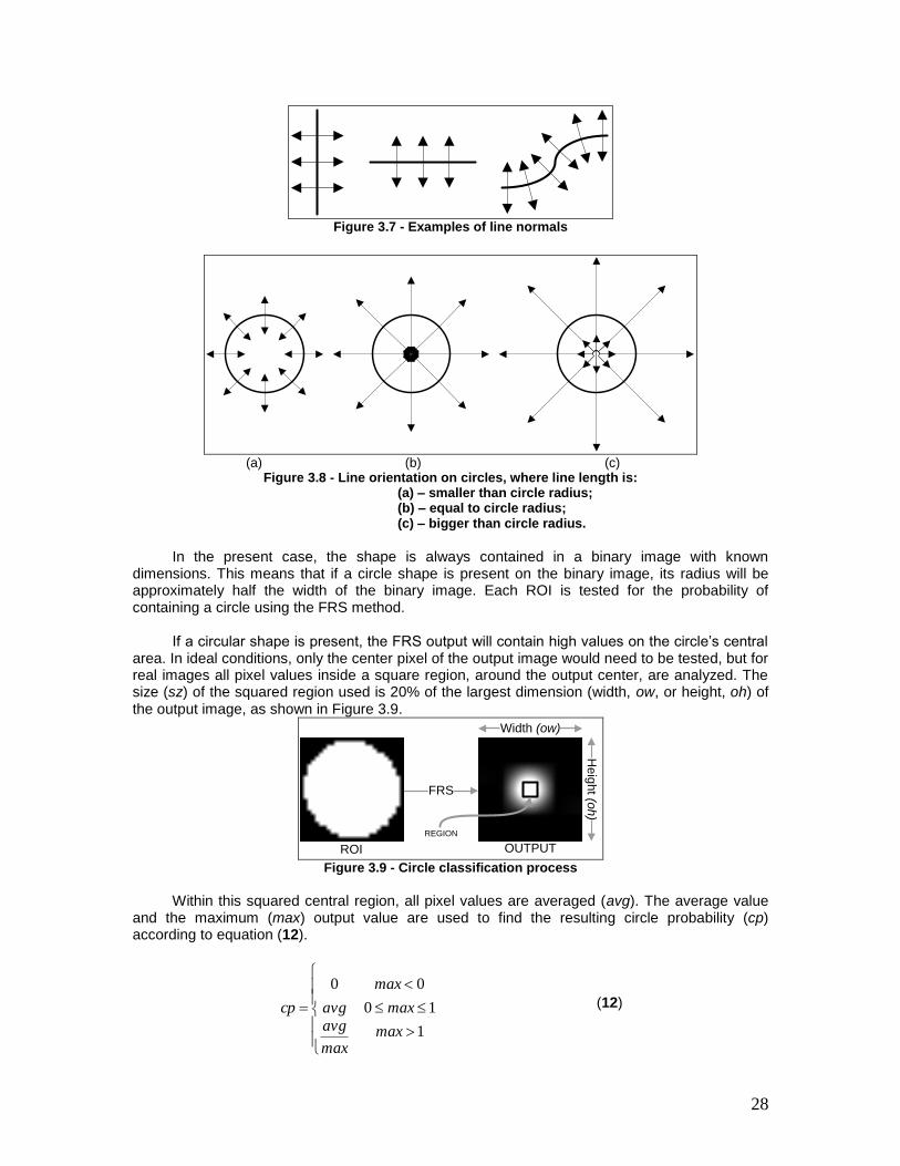
28
Figure 3.7 - Examples of line normals
(a) (b) (c)
Figure 3.8 - Line orientation on circles, where line length is: (a) – smaller than circle radius; (b) – equal to circle radius; (c) – bigger than circle radius.
In the present case, the shape is always contained in a binary image with known
dimensions. This means that if a circle shape is present on the binary image, its radius will be approximately half the width of the binary image. Each ROI is tested for the probability of containing a circle using the FRS method.
If a circular shape is present, the FRS output will contain high values on the circle‟s central
area. In ideal conditions, only the center pixel of the output image would need to be tested, but for real images all pixel values inside a square region, around the output center, are analyzed. The size (sz) of the squared region used is 20% of the largest dimension (width, ow, or height, oh) of the output image, as shown in Figure 3.9.
ROI
FRS
OUTPUT
REGION
He
igh
t (oh
)
Width (ow)
Figure 3.9 - Circle classification process
Within this squared central region, all pixel values are averaged (avg). The average value
and the maximum (max) output value are used to find the resulting circle probability (cp) according to equation (12).
1
10
00
max
max
max
max
avg
avgcp (12)
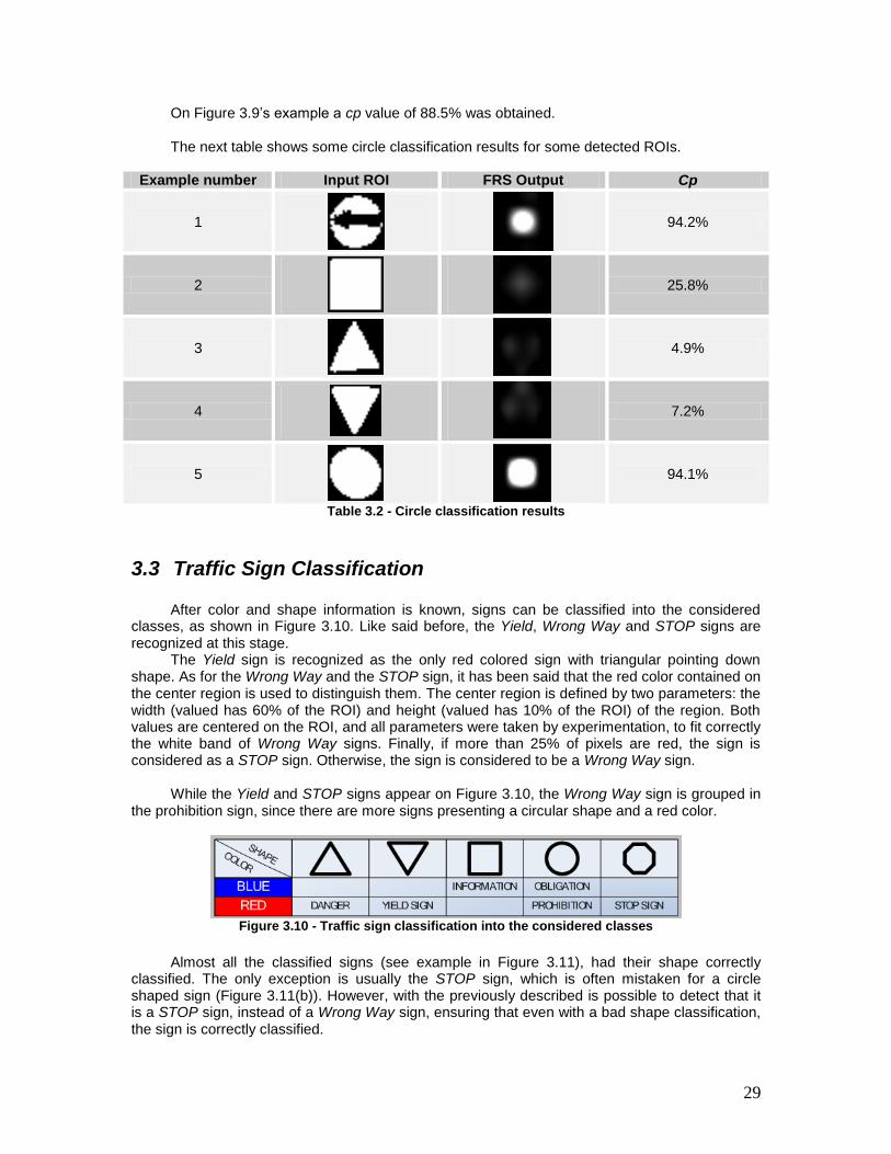
29
On Figure 3.9‟s example a cp value of 88.5% was obtained. The next table shows some circle classification results for some detected ROIs.
Example number Input ROI FRS Output Cp
1
94.2%
2
25.8%
3
4.9%
4
7.2%
5
94.1%
Table 3.2 - Circle classification results
3.3 Traffic Sign Classification After color and shape information is known, signs can be classified into the considered
classes, as shown in Figure 3.10. Like said before, the Yield, Wrong Way and STOP signs are recognized at this stage.
The Yield sign is recognized as the only red colored sign with triangular pointing down shape. As for the Wrong Way and the STOP sign, it has been said that the red color contained on the center region is used to distinguish them. The center region is defined by two parameters: the width (valued has 60% of the ROI) and height (valued has 10% of the ROI) of the region. Both values are centered on the ROI, and all parameters were taken by experimentation, to fit correctly the white band of Wrong Way signs. Finally, if more than 25% of pixels are red, the sign is considered as a STOP sign. Otherwise, the sign is considered to be a Wrong Way sign.
While the Yield and STOP signs appear on Figure 3.10, the Wrong Way sign is grouped in
the prohibition sign, since there are more signs presenting a circular shape and a red color.
Figure 3.10 - Traffic sign classification into the considered classes
Almost all the classified signs (see example in Figure 3.11), had their shape correctly
classified. The only exception is usually the STOP sign, which is often mistaken for a circle shaped sign (Figure 3.11(b)). However, with the previously described is possible to detect that it is a STOP sign, instead of a Wrong Way sign, ensuring that even with a bad shape classification, the sign is correctly classified.
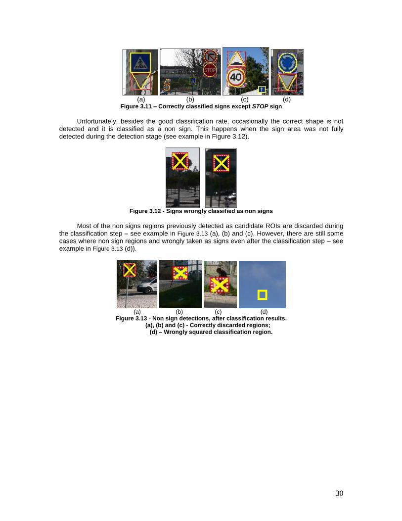
30
(a) (b) (c) (d)
Figure 3.11 – Correctly classified signs except STOP sign
Unfortunately, besides the good classification rate, occasionally the correct shape is not
detected and it is classified as a non sign. This happens when the sign area was not fully detected during the detection stage (see example in Figure 3.12).
Figure 3.12 - Signs wrongly classified as non signs
Most of the non signs regions previously detected as candidate ROIs are discarded during
the classification step – see example in Figure 3.13 (a), (b) and (c). However, there are still some cases where non sign regions and wrongly taken as signs even after the classification step – see example in Figure 3.13 (d)).
(a) (b) (c) (d)
Figure 3.13 - Non sign detections, after classification results. (a), (b) and (c) - Correctly discarded regions;
(d) – Wrongly squared classification region.
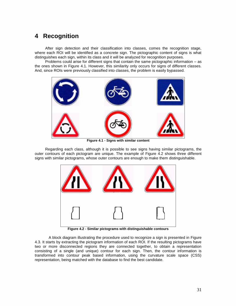
31
4 Recognition
After sign detection and their classification into classes, comes the recognition stage, where each ROI will be identified as a concrete sign. The pictographic content of signs is what distinguishes each sign, within its class and it will be analyzed for recognition purposes.
Problems could arise for different signs that contain the same pictographic information – as the ones shown in Figure 4.1. However, this similarity only occurs for signs of different classes. And, since ROIs were previously classified into classes, the problem is easily bypassed.
Figure 4.1 - Signs with similar content
Regarding each class, although it is possible to see signs having similar pictograms, the
outer contours of each pictogram are unique. The example of Figure 4.2 shows three different signs with similar pictograms, whose outer contours are enough to make them distinguishable.
Figure 4.2 - Similar pictograms with distinguishable contours
A block diagram illustrating the procedure used to recognize a sign is presented in Figure
4.3. It starts by extracting the pictogram information of each ROI. If the resulting pictograms have two or more disconnected regions they are connected together, to obtain a representation consisting of a single (and unique) contour for each sign. Then, the contour information is transformed into contour peak based information, using the curvature scale space (CSS) representation, being matched with the database to find the best candidate.
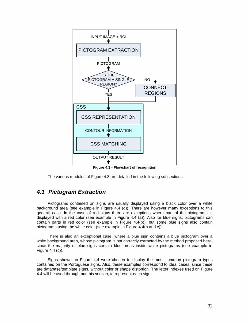
32
PICTOGRAM EXTRACTION
CONNECT
REGIONS
PICTOGRAM
INPUT IMAGE + ROI
CSS REPRESENTATION
CONTOUR INFORMATION
IS THE
PICTOGRAM A SINGLE
REGION?
NO
YES
CSS MATCHING
OUTPUT RESULT
CSS
Figure 4.3 - Flowchart of recognition
The various modules of Figure 4.3 are detailed in the following subsections.
4.1 Pictogram Extraction Pictograms contained on signs are usually displayed using a black color over a white
background area (see example in Figure 4.4 (d)). There are however many exceptions to this general case. In the case of red signs there are exceptions where part of the pictograms is displayed with a red color (see example in Figure 4.4 (a)). Also for blue signs, pictograms can contain parts in red color (see example in Figure 4.4(b)), but some blue signs also contain pictograms using the white color (see example in Figure 4.4(b and c)).
There is also an exceptional case, where a blue sign contains a blue pictogram over a
white background area, whose pictogram is not correctly extracted by the method proposed here, since the majority of blue signs contain blue areas inside white pictograms (see example in Figure 4.4 (c)).
Signs shown on Figure 4.4 were chosen to display the most common pictogram types
contained on the Portuguese signs. Also, these examples correspond to ideal cases, since these are database/template signs, without color or shape distortion. The letter indexes used on Figure 4.4 will be used through out this section, to represent each sign.
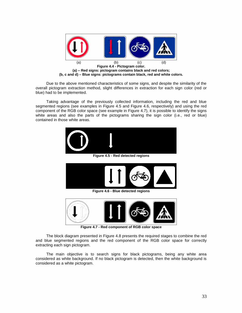
33
(a) (b) (c) (d)
Figure 4.4 - Pictogram color. (a) – Red signs: pictogram contains black and red colors;
(b, c and d) – Blue signs: pictograms contain black, red and white colors.
Due to the above mentioned characteristics of some signs, and despite the similarity of the
overall pictogram extraction method, slight differences in extraction for each sign color (red or blue) had to be implemented.
Taking advantage of the previously collected information, including the red and blue
segmented regions (see examples in Figure 4.5 and Figure 4.6, respectively) and using the red component of the RGB color space (see example in Figure 4.7), it is possible to identify the signs white areas and also the parts of the pictograms sharing the sign color (i.e., red or blue) contained in those white areas.
Figure 4.5 - Red detected regions
Figure 4.6 - Blue detected regions
Figure 4.7 - Red component of RGB color space
The block diagram presented in Figure 4.8 presents the required stages to combine the red
and blue segmented regions and the red component of the RGB color space for correctly extracting each sign pictogram.
The main objective is to search signs for black pictograms, being any white area
considered as white background. If no black pictogram is detected, then the white background is considered as a white pictogram.
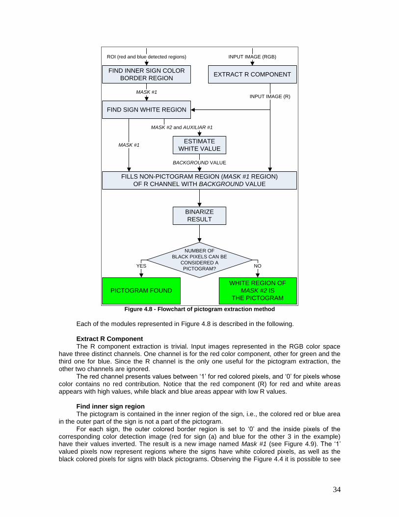
34
FIND SIGN WHITE REGION
WHITE REGION OF
MASK #2 IS
THE PICTOGRAM
MASK #2 and AUXILIAR #1
MASK #1
ESTIMATE
WHITE VALUE
BACKGROUND VALUE
NUMBER OF
BLACK PIXELS CAN BE
CONSIDERED A
PICTOGRAM?NOYES
FILLS NON-PICTOGRAM REGION (MASK #1 REGION)
OF R CHANNEL WITH BACKGROUND VALUE
EXTRACT R COMPONENT
INPUT IMAGE (RGB)
BINARIZE
RESULT
MASK #1
PICTOGRAM FOUND
INPUT IMAGE (R)
FIND INNER SIGN COLOR
BORDER REGION
ROI (red and blue detected regions)
Figure 4.8 - Flowchart of pictogram extraction method
Each of the modules represented in Figure 4.8 is described in the following. Extract R Component The R component extraction is trivial. Input images represented in the RGB color space
have three distinct channels. One channel is for the red color component, other for green and the third one for blue. Since the R channel is the only one useful for the pictogram extraction, the other two channels are ignored.
The red channel presents values between „1‟ for red colored pixels, and „0‟ for pixels whose color contains no red contribution. Notice that the red component (R) for red and white areas appears with high values, while black and blue areas appear with low R values.
Find inner sign region The pictogram is contained in the inner region of the sign, i.e., the colored red or blue area
in the outer part of the sign is not a part of the pictogram. For each sign, the outer colored border region is set to „0‟ and the inside pixels of the
corresponding color detection image (red for sign (a) and blue for the other 3 in the example) have their values inverted. The result is a new image named Mask #1 (see Figure 4.9). The „1‟ valued pixels now represent regions where the signs have white colored pixels, as well as the black colored pixels for signs with black pictograms. Observing the Figure 4.4 it is possible to see
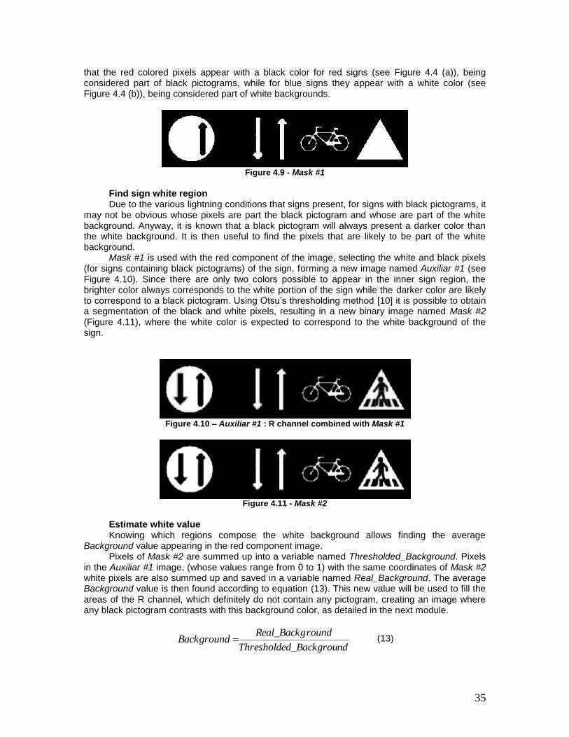
35
that the red colored pixels appear with a black color for red signs (see Figure 4.4 (a)), being considered part of black pictograms, while for blue signs they appear with a white color (see Figure 4.4 (b)), being considered part of white backgrounds.
Figure 4.9 - Mask #1
Find sign white region Due to the various lightning conditions that signs present, for signs with black pictograms, it
may not be obvious whose pixels are part the black pictogram and whose are part of the white background. Anyway, it is known that a black pictogram will always present a darker color than the white background. It is then useful to find the pixels that are likely to be part of the white background.
Mask #1 is used with the red component of the image, selecting the white and black pixels (for signs containing black pictograms) of the sign, forming a new image named Auxiliar #1 (see Figure 4.10). Since there are only two colors possible to appear in the inner sign region, the brighter color always corresponds to the white portion of the sign while the darker color are likely to correspond to a black pictogram. Using Otsu‟s thresholding method [10] it is possible to obtain a segmentation of the black and white pixels, resulting in a new binary image named Mask #2 (Figure 4.11), where the white color is expected to correspond to the white background of the sign.
Figure 4.10 – Auxiliar #1 : R channel combined with Mask #1
Figure 4.11 - Mask #2
Estimate white value Knowing which regions compose the white background allows finding the average
Background value appearing in the red component image. Pixels of Mask #2 are summed up into a variable named Thresholded_Background. Pixels
in the Auxiliar #1 image, (whose values range from 0 to 1) with the same coordinates of Mask #2 white pixels are also summed up and saved in a variable named Real_Background. The average Background value is then found according to equation (13). This new value will be used to fill the areas of the R channel, which definitely do not contain any pictogram, creating an image where any black pictogram contrasts with this background color, as detailed in the next module.
ndd_BackgrouThresholde
roundReal_BackgBackground (13)
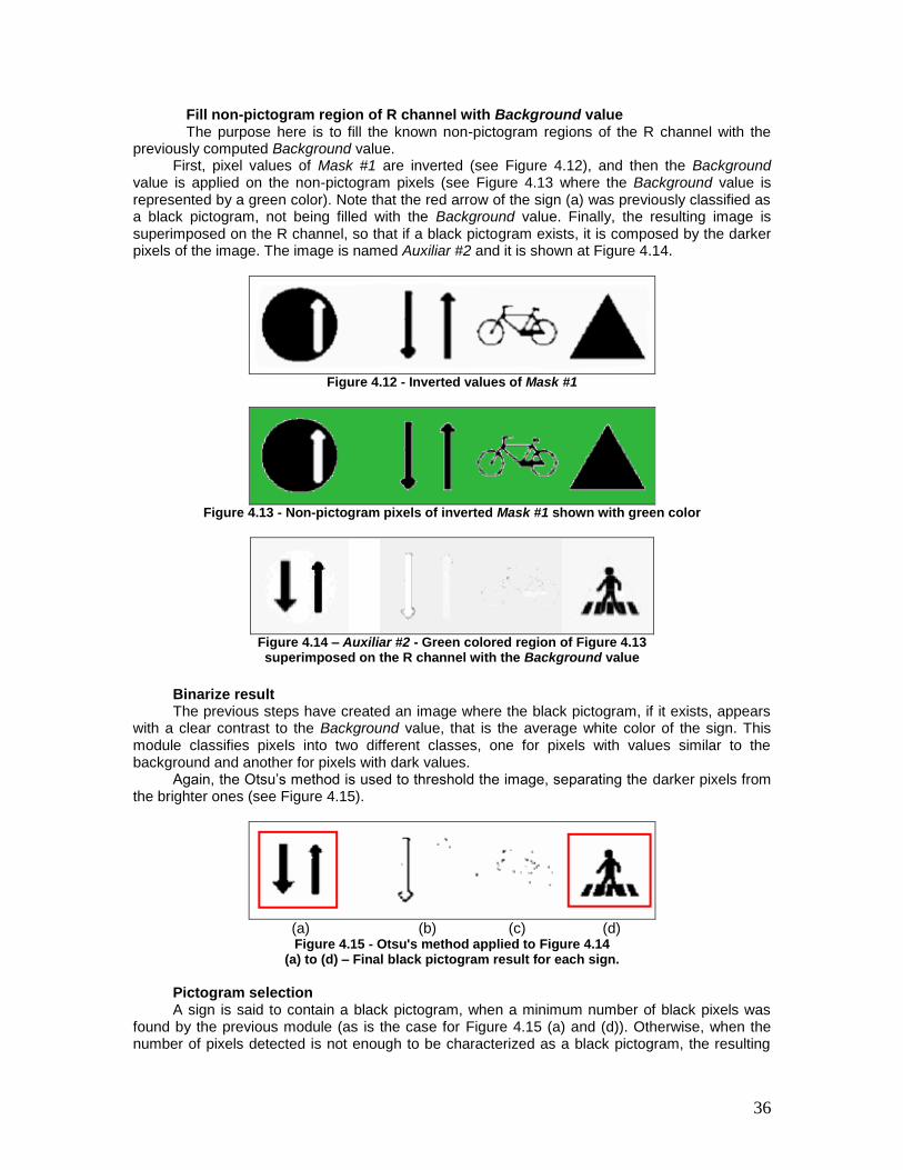
36
Fill non-pictogram region of R channel with Background value The purpose here is to fill the known non-pictogram regions of the R channel with the
previously computed Background value. First, pixel values of Mask #1 are inverted (see Figure 4.12), and then the Background
value is applied on the non-pictogram pixels (see Figure 4.13 where the Background value is represented by a green color). Note that the red arrow of the sign (a) was previously classified as a black pictogram, not being filled with the Background value. Finally, the resulting image is superimposed on the R channel, so that if a black pictogram exists, it is composed by the darker pixels of the image. The image is named Auxiliar #2 and it is shown at Figure 4.14.
Figure 4.12 - Inverted values of Mask #1
Figure 4.13 - Non-pictogram pixels of inverted Mask #1 shown with green color
Figure 4.14 – Auxiliar #2 - Green colored region of Figure 4.13 superimposed on the R channel with the Background value
Binarize result The previous steps have created an image where the black pictogram, if it exists, appears
with a clear contrast to the Background value, that is the average white color of the sign. This module classifies pixels into two different classes, one for pixels with values similar to the background and another for pixels with dark values.
Again, the Otsu‟s method is used to threshold the image, separating the darker pixels from the brighter ones (see Figure 4.15).
(a) (b) (c) (d)
Figure 4.15 - Otsu's method applied to Figure 4.14 (a) to (d) – Final black pictogram result for each sign.
Pictogram selection A sign is said to contain a black pictogram, when a minimum number of black pixels was
found by the previous module (as is the case for Figure 4.15 (a) and (d)). Otherwise, when the number of pixels detected is not enough to be characterized as a black pictogram, the resulting
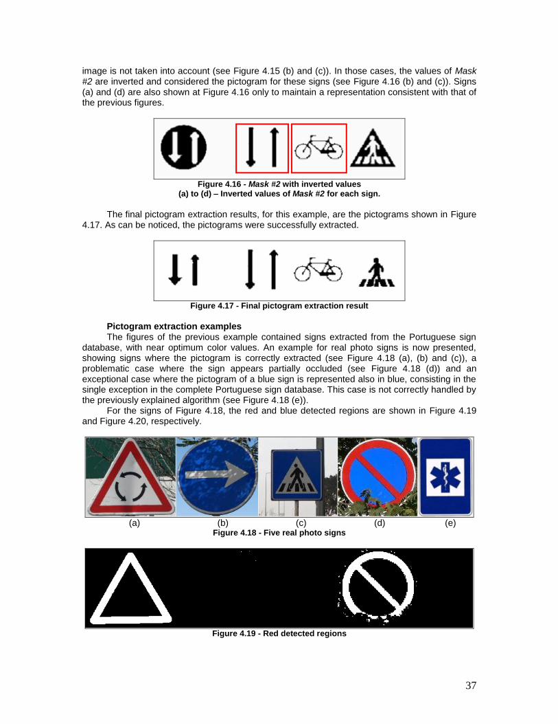
37
image is not taken into account (see Figure 4.15 (b) and (c)). In those cases, the values of Mask #2 are inverted and considered the pictogram for these signs (see Figure 4.16 (b) and (c)). Signs (a) and (d) are also shown at Figure 4.16 only to maintain a representation consistent with that of the previous figures.
Figure 4.16 - Mask #2 with inverted values
(a) to (d) – Inverted values of Mask #2 for each sign.
The final pictogram extraction results, for this example, are the pictograms shown in Figure
4.17. As can be noticed, the pictograms were successfully extracted.
Figure 4.17 - Final pictogram extraction result
Pictogram extraction examples The figures of the previous example contained signs extracted from the Portuguese sign
database, with near optimum color values. An example for real photo signs is now presented, showing signs where the pictogram is correctly extracted (see Figure 4.18 (a), (b) and (c)), a problematic case where the sign appears partially occluded (see Figure 4.18 (d)) and an exceptional case where the pictogram of a blue sign is represented also in blue, consisting in the single exception in the complete Portuguese sign database. This case is not correctly handled by the previously explained algorithm (see Figure 4.18 (e)).
For the signs of Figure 4.18, the red and blue detected regions are shown in Figure 4.19 and Figure 4.20, respectively.
(a) (b) (c) (d) (e)
Figure 4.18 - Five real photo signs
Figure 4.19 - Red detected regions
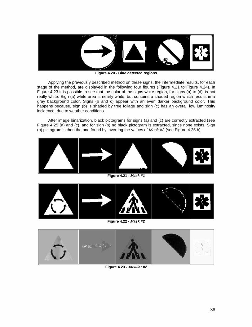
38
Figure 4.20 - Blue detected regions
Applying the previously described method on these signs, the intermediate results, for each
stage of the method, are displayed in the following four figures (Figure 4.21 to Figure 4.24). In Figure 4.23 it is possible to see that the color of the signs white region, for signs (a) to (d), is not really white. Sign (a) white area is nearly white, but contains a shaded region which results in a gray background color. Signs (b and c) appear with an even darker background color. This happens because, sign (b) is shaded by tree foliage and sign (c) has an overall low luminosity incidence, due to weather conditions.
After image binarization, black pictograms for signs (a) and (c) are correctly extracted (see
Figure 4.25 (a) and (c), and for sign (b) no black pictogram is extracted, since none exists. Sign (b) pictogram is then the one found by inverting the values of Mask #2 (see Figure 4.25 b).
Figure 4.21 - Mask #1
Figure 4.22 - Mask #2
Figure 4.23 - Auxiliar #2
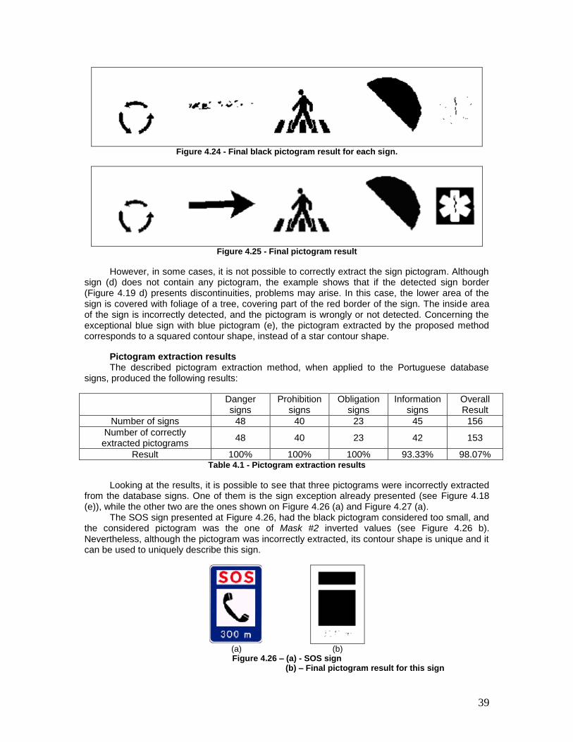
39
Figure 4.24 - Final black pictogram result for each sign.
Figure 4.25 - Final pictogram result
However, in some cases, it is not possible to correctly extract the sign pictogram. Although sign (d) does not contain any pictogram, the example shows that if the detected sign border (Figure 4.19 d) presents discontinuities, problems may arise. In this case, the lower area of the sign is covered with foliage of a tree, covering part of the red border of the sign. The inside area of the sign is incorrectly detected, and the pictogram is wrongly or not detected. Concerning the exceptional blue sign with blue pictogram (e), the pictogram extracted by the proposed method corresponds to a squared contour shape, instead of a star contour shape.
Pictogram extraction results The described pictogram extraction method, when applied to the Portuguese database
signs, produced the following results:
Danger signs
Prohibition signs
Obligation signs
Information signs
Overall Result
Number of signs 48 40 23 45 156
Number of correctly extracted pictograms
48 40 23 42 153
Result 100% 100% 100% 93.33% 98.07% Table 4.1 - Pictogram extraction results
Looking at the results, it is possible to see that three pictograms were incorrectly extracted from the database signs. One of them is the sign exception already presented (see Figure 4.18 (e)), while the other two are the ones shown on Figure 4.26 (a) and Figure 4.27 (a).
The SOS sign presented at Figure 4.26, had the black pictogram considered too small, and the considered pictogram was the one of Mask #2 inverted values (see Figure 4.26 b). Nevertheless, although the pictogram was incorrectly extracted, its contour shape is unique and it can be used to uniquely describe this sign.
(a) (b)
Figure 4.26 – (a) - SOS sign (b) – Final pictogram result for this sign
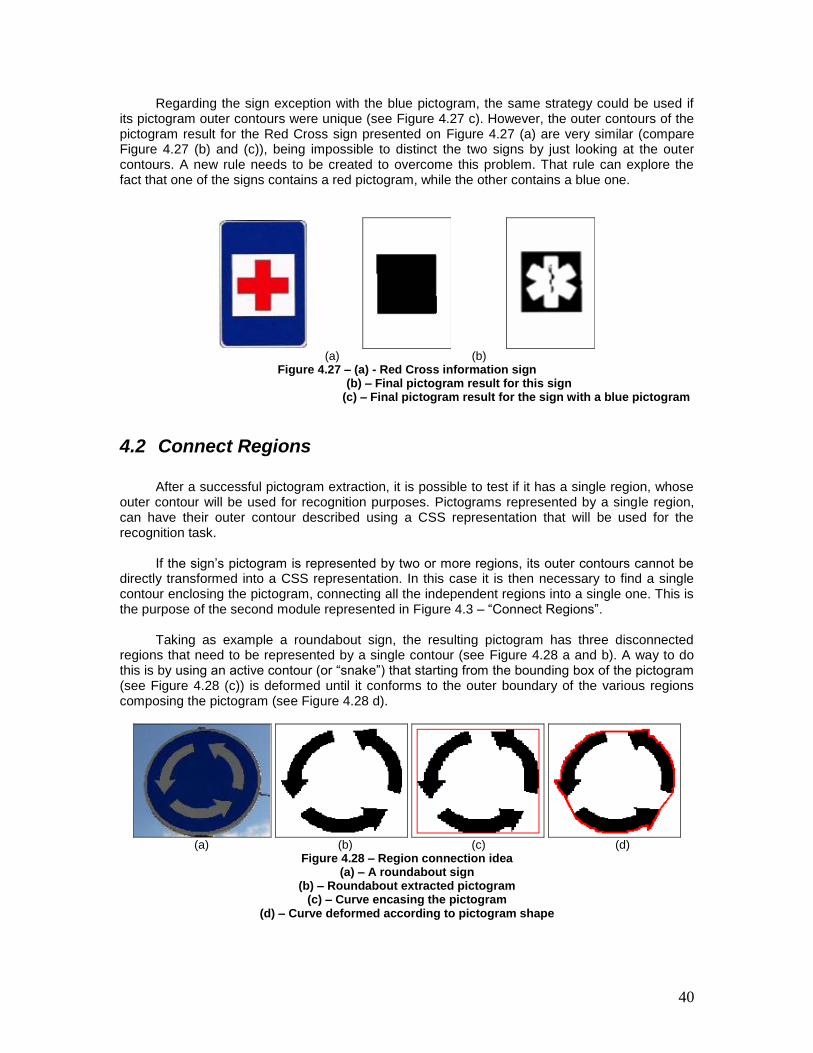
40
Regarding the sign exception with the blue pictogram, the same strategy could be used if its pictogram outer contours were unique (see Figure 4.27 c). However, the outer contours of the pictogram result for the Red Cross sign presented on Figure 4.27 (a) are very similar (compare Figure 4.27 (b) and (c)), being impossible to distinct the two signs by just looking at the outer contours. A new rule needs to be created to overcome this problem. That rule can explore the fact that one of the signs contains a red pictogram, while the other contains a blue one.
(a) (b)
Figure 4.27 – (a) - Red Cross information sign (b) – Final pictogram result for this sign
(c) – Final pictogram result for the sign with a blue pictogram
4.2 Connect Regions
After a successful pictogram extraction, it is possible to test if it has a single region, whose
outer contour will be used for recognition purposes. Pictograms represented by a single region, can have their outer contour described using a CSS representation that will be used for the recognition task.
If the sign‟s pictogram is represented by two or more regions, its outer contours cannot be
directly transformed into a CSS representation. In this case it is then necessary to find a single contour enclosing the pictogram, connecting all the independent regions into a single one. This is the purpose of the second module represented in Figure 4.3 – “Connect Regions”.
Taking as example a roundabout sign, the resulting pictogram has three disconnected
regions that need to be represented by a single contour (see Figure 4.28 a and b). A way to do this is by using an active contour (or “snake”) that starting from the bounding box of the pictogram (see Figure 4.28 (c)) is deformed until it conforms to the outer boundary of the various regions composing the pictogram (see Figure 4.28 d).
(a) (b) (c) (d)
Figure 4.28 – Region connection idea (a) – A roundabout sign
(b) – Roundabout extracted pictogram (c) – Curve encasing the pictogram
(d) – Curve deformed according to pictogram shape
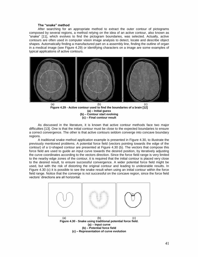
41
The “snake” method After searching for an appropriate method to extract the outer contour of pictograms
composed by several regions, a method relying on the idea of an active contour, also known as “snake” [11], which evolves to find the pictogram boundaries, was selected. Actually, active contours are often used in computer vision image analysis to detect, locate and describe object shapes. Automatically finding a manufactured part on a assembly line, finding the outline of organ in a medical image (see Figure 4.29) or identifying characters on a image are some examples of typical applications of active contours.
(a) (b) (c) Figure 4.29 - Active contour used to find the boundaries of a brain [12]
(a) – Initial guess (b) – Contour start evolving
(c) – Final contour result
As discussed in the literature, it is known that active contour methods face two major
difficulties [13]. One is that the initial contour must be close to the expected boundaries to ensure a correct convergence. The other is that active contours seldom converge into concave boundary regions.
A traditional snake method application example is presented in Figure 4.30, to illustrate the previously mentioned problems. A potential force field (vectors pointing towards the edge of the contour) of a U-shaped contour are presented at Figure 4.30 (b). The vectors that compose this force field are used to guide an input curve towards the desired position, by iteratively adjusting the curve coordinates according to the vectors direction. Since the force field range is very limited to the nearby edge zones of the contour, it is required that the initial contour is placed very close to the desired result, to ensure successful convergence. A wider potential force field might be used, but with the risk of distorting the original contour and leading to undesirable results. In Figure 4.30 (c) it is possible to see the snake result when using an initial contour within the force field range. Notice that the converge is not successful on the concave region, since the force field vectors‟ directions are all horizontal.
(a) (b) (c)
Figure 4.30 - Snake using traditional potential force field. (a) – Input curve
(b) – Potential force field (c) – Representation of curve evolution
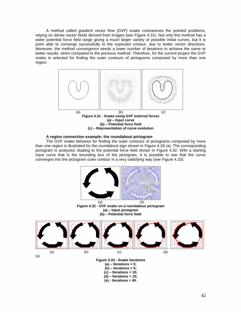
42
A method called gradient vector flow (GVF) snake contravenes the pointed problems, relying on dense vector fields derived from images (see Figure 4.31). Not only this method has a wider potential force field range giving a much larger variety of possible initial curves, but it is point able to converge successfully to the expected contour, due to better vector directions. Moreover, the method convergence needs a lower number of iterations to achieve the same or better results, when compared to the previous method. Therefore, for the current project the GVF snake is selected for finding the outer contours of pictograms composed by more than one region.
(a) (b) (c)
Figure 4.31 - Snake using GVF external forces (a) – Input curve
(b) – Potential force field (c) – Representation of curve evolution
A region connection example: the roundabout pictogram The GVF snake behavior for finding the outer contours of pictograms composed by more
than one region is illustrated for the roundabout sign shown in Figure 4.28 (a). The corresponding pictogram is analyzed, leading to the potential force field shown in Figure 4.32. With a starting input curve that is the bounding box of the pictogram, it is possible to see that the curve converges into the pictogram outer contour in a very satisfying way (see Figure 4.33).
(a) (b)
Figure 4.32 - GVF snake on a roundabout pictogram (a) – Input pictogram
(b) – Potential force field
… (a) (b) (c) (d)
(e) Figure 4.33 - Snake iterations
(a) – Iterations = 0; (b) – Iterations = 5; (c) – Iterations = 10; (d) – Iterations = 15; (e) - Iterations = 40.
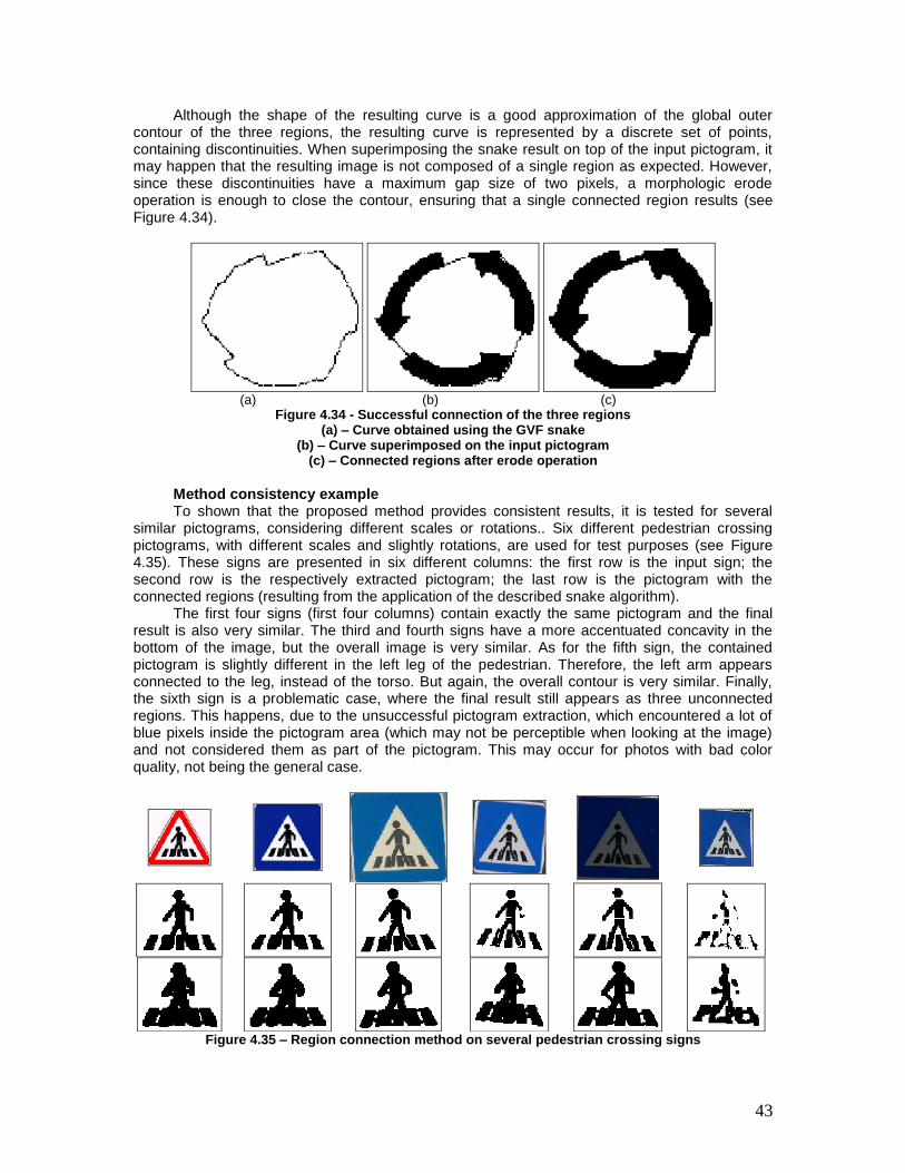
43
Although the shape of the resulting curve is a good approximation of the global outer contour of the three regions, the resulting curve is represented by a discrete set of points, containing discontinuities. When superimposing the snake result on top of the input pictogram, it may happen that the resulting image is not composed of a single region as expected. However, since these discontinuities have a maximum gap size of two pixels, a morphologic erode operation is enough to close the contour, ensuring that a single connected region results (see Figure 4.34).
(a) (b) (c)
Figure 4.34 - Successful connection of the three regions (a) – Curve obtained using the GVF snake
(b) – Curve superimposed on the input pictogram (c) – Connected regions after erode operation
Method consistency example To shown that the proposed method provides consistent results, it is tested for several
similar pictograms, considering different scales or rotations.. Six different pedestrian crossing pictograms, with different scales and slightly rotations, are used for test purposes (see Figure 4.35). These signs are presented in six different columns: the first row is the input sign; the second row is the respectively extracted pictogram; the last row is the pictogram with the connected regions (resulting from the application of the described snake algorithm).
The first four signs (first four columns) contain exactly the same pictogram and the final result is also very similar. The third and fourth signs have a more accentuated concavity in the bottom of the image, but the overall image is very similar. As for the fifth sign, the contained pictogram is slightly different in the left leg of the pedestrian. Therefore, the left arm appears connected to the leg, instead of the torso. But again, the overall contour is very similar. Finally, the sixth sign is a problematic case, where the final result still appears as three unconnected regions. This happens, due to the unsuccessful pictogram extraction, which encountered a lot of blue pixels inside the pictogram area (which may not be perceptible when looking at the image) and not considered them as part of the pictogram. This may occur for photos with bad color quality, not being the general case.
Figure 4.35 – Region connection method on several pedestrian crossing signs
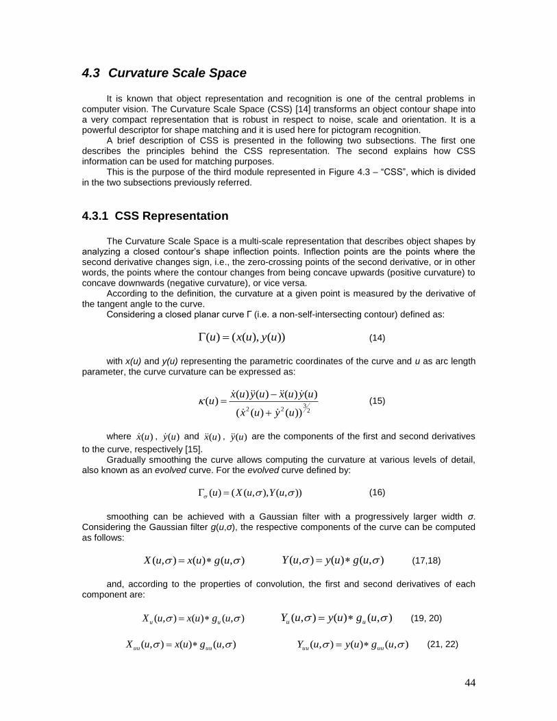
44
4.3 Curvature Scale Space
It is known that object representation and recognition is one of the central problems in computer vision. The Curvature Scale Space (CSS) [14] transforms an object contour shape into a very compact representation that is robust in respect to noise, scale and orientation. It is a powerful descriptor for shape matching and it is used here for pictogram recognition.
A brief description of CSS is presented in the following two subsections. The first one describes the principles behind the CSS representation. The second explains how CSS information can be used for matching purposes.
This is the purpose of the third module represented in Figure 4.3 – “CSS”, which is divided in the two subsections previously referred.
4.3.1 CSS Representation
The Curvature Scale Space is a multi-scale representation that describes object shapes by
analyzing a closed contour‟s shape inflection points. Inflection points are the points where the second derivative changes sign, i.e., the zero-crossing points of the second derivative, or in other words, the points where the contour changes from being concave upwards (positive curvature) to concave downwards (negative curvature), or vice versa.
According to the definition, the curvature at a given point is measured by the derivative of the tangent angle to the curve.
Considering a closed planar curve Г (i.e. a non-self-intersecting contour) defined as:
))(),(()( uyuxu (14)
with x(u) and y(u) representing the parametric coordinates of the curve and u as arc length
parameter, the curve curvature can be expressed as:
23
22 ))()((
)()()()()(
uyux
uyuxuyuxu
(15)
where )(ux , )(uy and )(ux , )(uy are the components of the first and second derivatives
to the curve, respectively [15]. Gradually smoothing the curve allows computing the curvature at various levels of detail,
also known as an evolved curve. For the evolved curve defined by:
)),(),,(()( uYuXu (16)
smoothing can be achieved with a Gaussian filter with a progressively larger width σ.
Considering the Gaussian filter g(u,σ), the respective components of the curve can be computed as follows:
),()(),( uguxuX ),()(),( uguyuY (17,18)
and, according to the properties of convolution, the first and second derivatives of each
component are:
),()(),( uguxuX uu ),()(),( uguyuY uu (19, 20)
),()(),( uguxuX uuuu ),()(),( uguyuY uuuu (21, 22)
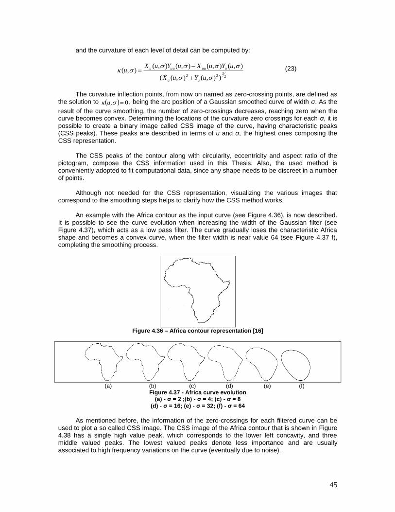
45
and the curvature of each level of detail can be computed by:
23
22 )),(),((
),(),(),(),(),(
uYuX
uYuXuYuXu
uu
uuuuuu
(23)
The curvature inflection points, from now on named as zero-crossing points, are defined as
the solution to 0, u , being the arc position of a Gaussian smoothed curve of width σ. As the
result of the curve smoothing, the number of zero-crossings decreases, reaching zero when the curve becomes convex. Determining the locations of the curvature zero crossings for each σ, it is possible to create a binary image called CSS image of the curve, having characteristic peaks (CSS peaks). These peaks are described in terms of u and σ, the highest ones composing the CSS representation.
The CSS peaks of the contour along with circularity, eccentricity and aspect ratio of the
pictogram, compose the CSS information used in this Thesis. Also, the used method is conveniently adopted to fit computational data, since any shape needs to be discreet in a number of points.
Although not needed for the CSS representation, visualizing the various images that
correspond to the smoothing steps helps to clarify how the CSS method works. An example with the Africa contour as the input curve (see Figure 4.36), is now described.
It is possible to see the curve evolution when increasing the width of the Gaussian filter (see Figure 4.37), which acts as a low pass filter. The curve gradually loses the characteristic Africa shape and becomes a convex curve, when the filter width is near value 64 (see Figure 4.37 f), completing the smoothing process.
Figure 4.36 – Africa contour representation [16]
(a) (b) (c) (d) (e) (f)
Figure 4.37 - Africa curve evolution (a) - σ = 2 ;(b) - σ = 4; (c) - σ = 8
(d) - σ = 16; (e) - σ = 32; (f) - σ = 64
As mentioned before, the information of the zero-crossings for each filtered curve can be
used to plot a so called CSS image. The CSS image of the Africa contour that is shown in Figure 4.38 has a single high value peak, which corresponds to the lower left concavity, and three middle valued peaks. The lowest valued peaks denote less importance and are usually associated to high frequency variations on the curve (eventually due to noise).
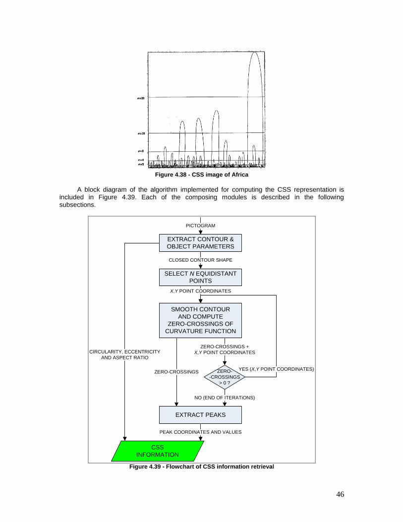
46
Figure 4.38 - CSS image of Africa
A block diagram of the algorithm implemented for computing the CSS representation is
included in Figure 4.39. Each of the composing modules is described in the following subsections.
EXTRACT CONTOUR &
OBJECT PARAMETERS
SELECT N EQUIDISTANT
POINTS
CLOSED CONTOUR SHAPE
PICTOGRAM
X,Y POINT COORDINATES
SMOOTH CONTOUR
AND COMPUTE
ZERO-CROSSINGS OF
CURVATURE FUNCTION
YES (X,Y POINT COORDINATES)ZERO-CROSSINGS ZERO-
-CROSSINGS
> 0 ?
ZERO-CROSSINGS +
X,Y POINT COORDINATES
EXTRACT PEAKS
NO (END OF ITERATiONS)
PEAK COORDINATES AND VALUES
CIRCULARITY, ECCENTRICITY
AND ASPECT RATIO
CSS
INFORMATION
Figure 4.39 - Flowchart of CSS information retrieval
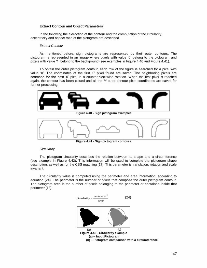
47
Extract Contour and Object Parameters In the following the extraction of the contour and the computation of the circularity,
eccentricity and aspect ratio of the pictogram are described. Extract Contour As mentioned before, sign pictograms are represented by their outer contours. The
pictogram is represented in an image where pixels with value „0‟ belong to the pictogram and pixels with value „1‟ belong to the background (see examples in Figure 4.40 and Figure 4.41).
To obtain the outer pictogram contour, each row of the figure is searched for a pixel with
value „0‟. The coordinates of the first „0‟ pixel found are saved. The neighboring pixels are searched for the next „0‟ pixel in a counter-clockwise rotation. When the first pixel is reached again, the contour has been closed and all the M outer contour pixel coordinates are saved for further processing.
Figure 4.40 - Sign pictogram examples
Figure 4.41 - Sign pictogram contours
Circularity The pictogram circularity describes the relation between its shape and a circumference
(see example in Figure 4.42). This information will be used to complete the pictogram shape description, as well as for the CSS matching [17]. This parameter is translation, rotation and scale invariant.
The circularity value is computed using the perimeter and area information, according to
equation (24). The perimeter is the number of pixels that compose the outer pictogram contour. The pictogram area is the number of pixels belonging to the perimeter or contained inside that perimeter [18].
area
perimeter 2
ycircularit (24)
(a) (b)
Figure 4.42 - Circularity example (a) – Input Pictogram
(b) – Pictogram comparison with a circumference
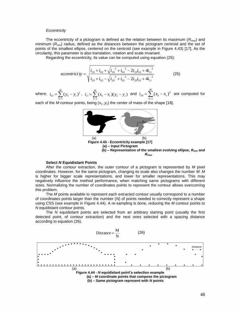
48
Eccentricity
The eccentricity of a pictogram is defined as the relation between its maximum (Rmax) and
minimum (Rmin) radius, defined as the distances between the pictogram centroid and the set of points of the smallest ellipse, centered on the centroid (see example in Figure 4.43) [17]. As the circularity, this parameter is also translation, rotation and scale invariant.
Regarding the eccentricity, its value can be computed using equation (25):
2
110220
2
02
2
200220
2
110220
2
02
2
200220
42
42
iiiiiii
iiiiiiityeccentrici
(25)
where,
M
k
ck yyi1
2
02 )( ,
M
k
ckck yyxxi1
11 ))(( and
M
k
ck xxi1
2
20 )( are computed for
each of the M contour points, being (xc, yc) the center of mass of the shape [18].
(a) (b)
Figure 4.43 - Eccentricity example [17] (a) – Input Pictogram
(b) – Representation of the smallest evolving ellipse, Rmin and Rmax
Select N Equidistant Points After the contour extraction, the outer contour of a pictogram is represented by M pixel
coordinates. However, for the same pictogram, changing its scale also changes the number M: M is higher for bigger scale representations, and lower for smaller representations. This may negatively influence the method performance, when matching same pictograms with different sizes. Normalizing the number of coordinates points to represent the contour allows overcoming this problem.
The M points available to represent each extracted contour usually correspond to a number of coordinates points larger than the number (N) of points needed to correctly represent a shape using CSS (see example in Figure 4.44). A re-sampling is done, reducing the M contour points to N equidistant contour points.
The N equidistant points are selected from an arbitrary starting point (usually the first detected point, of contour extraction) and the next ones selected with a spacing distance according to equation (26).
N
MDistance (26)
Distance
(a) (b)
Figure 4.44 - N equidistant point‟s selection example (a) – M coordinate points that compose the pictogram
(b) – Same pictogram represent with N points
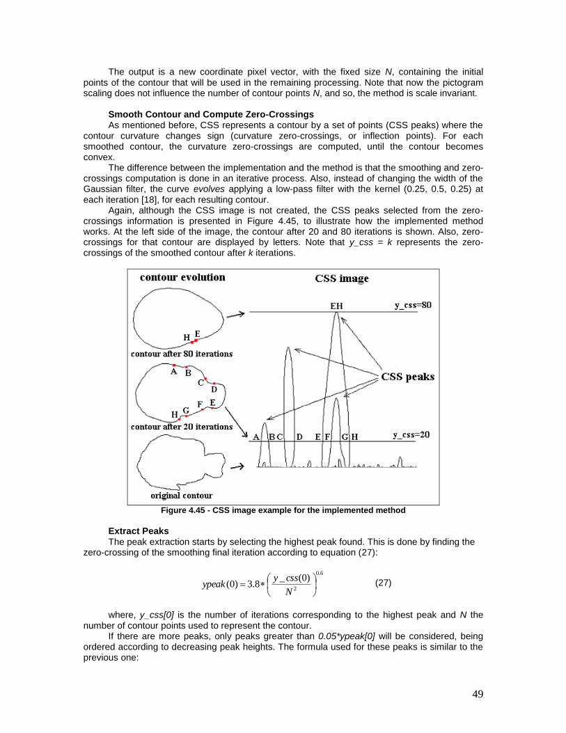
49
The output is a new coordinate pixel vector, with the fixed size N, containing the initial points of the contour that will be used in the remaining processing. Note that now the pictogram scaling does not influence the number of contour points N, and so, the method is scale invariant.
Smooth Contour and Compute Zero-Crossings As mentioned before, CSS represents a contour by a set of points (CSS peaks) where the
contour curvature changes sign (curvature zero-crossings, or inflection points). For each smoothed contour, the curvature zero-crossings are computed, until the contour becomes convex.
The difference between the implementation and the method is that the smoothing and zero-crossings computation is done in an iterative process. Also, instead of changing the width of the Gaussian filter, the curve evolves applying a low-pass filter with the kernel (0.25, 0.5, 0.25) at each iteration [18], for each resulting contour.
Again, although the CSS image is not created, the CSS peaks selected from the zero-crossings information is presented in Figure 4.45, to illustrate how the implemented method works. At the left side of the image, the contour after 20 and 80 iterations is shown. Also, zero-crossings for that contour are displayed by letters. Note that y_css = k represents the zero-crossings of the smoothed contour after k iterations.
Figure 4.45 - CSS image example for the implemented method
Extract Peaks The peak extraction starts by selecting the highest peak found. This is done by finding the
zero-crossing of the smoothing final iteration according to equation (27):
6.0
2
)0(_8.3)0(
N
cssyypeak (27)
where, y_css[0] is the number of iterations corresponding to the highest peak and N the
number of contour points used to represent the contour. If there are more peaks, only peaks greater than 0.05*ypeak[0] will be considered, being
ordered according to decreasing peak heights. The formula used for these peaks is similar to the previous one:
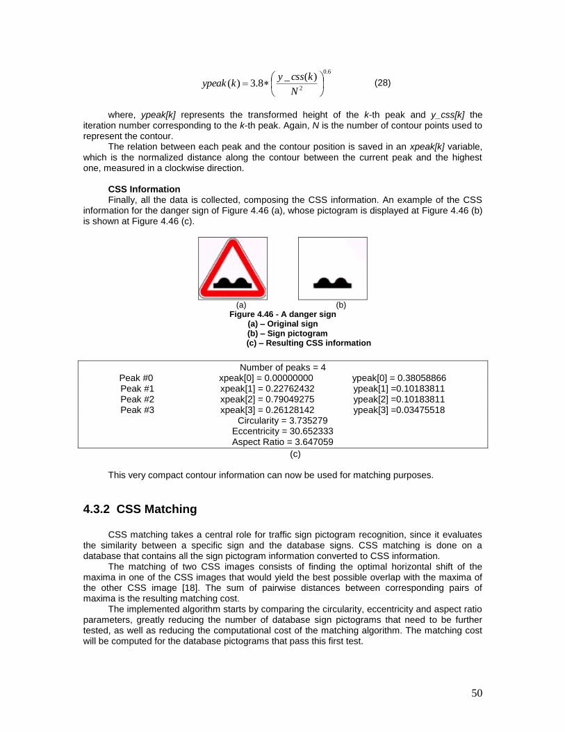
50
6.0
2
)(_8.3)(
N
kcssykypeak (28)
where, ypeak[k] represents the transformed height of the k-th peak and y_css[k] the
iteration number corresponding to the k-th peak. Again, N is the number of contour points used to represent the contour.
The relation between each peak and the contour position is saved in an xpeak[k] variable, which is the normalized distance along the contour between the current peak and the highest one, measured in a clockwise direction.
CSS Information Finally, all the data is collected, composing the CSS information. An example of the CSS
information for the danger sign of Figure 4.46 (a), whose pictogram is displayed at Figure 4.46 (b) is shown at Figure 4.46 (c).
(a) (b)
Figure 4.46 - A danger sign (a) – Original sign
(b) – Sign pictogram (c) – Resulting CSS information
Number of peaks = 4
Peak #0 xpeak[0] = 0.00000000 ypeak[0] = 0.38058866 Peak #1 xpeak[1] = 0.22762432 ypeak[1] =0.10183811 Peak #2 xpeak[2] = 0.79049275 ypeak[2] =0.10183811 Peak #3 xpeak[3] = 0.26128142 ypeak[3] =0.03475518
Circularity = 3.735279 Eccentricity = 30.652333 Aspect Ratio = 3.647059
(c) This very compact contour information can now be used for matching purposes.
4.3.2 CSS Matching CSS matching takes a central role for traffic sign pictogram recognition, since it evaluates
the similarity between a specific sign and the database signs. CSS matching is done on a database that contains all the sign pictogram information converted to CSS information.
The matching of two CSS images consists of finding the optimal horizontal shift of the maxima in one of the CSS images that would yield the best possible overlap with the maxima of the other CSS image [18]. The sum of pairwise distances between corresponding pairs of maxima is the resulting matching cost.
The implemented algorithm starts by comparing the circularity, eccentricity and aspect ratio parameters, greatly reducing the number of database sign pictograms that need to be further tested, as well as reducing the computational cost of the matching algorithm. The matching cost will be computed for the database pictograms that pass this first test.
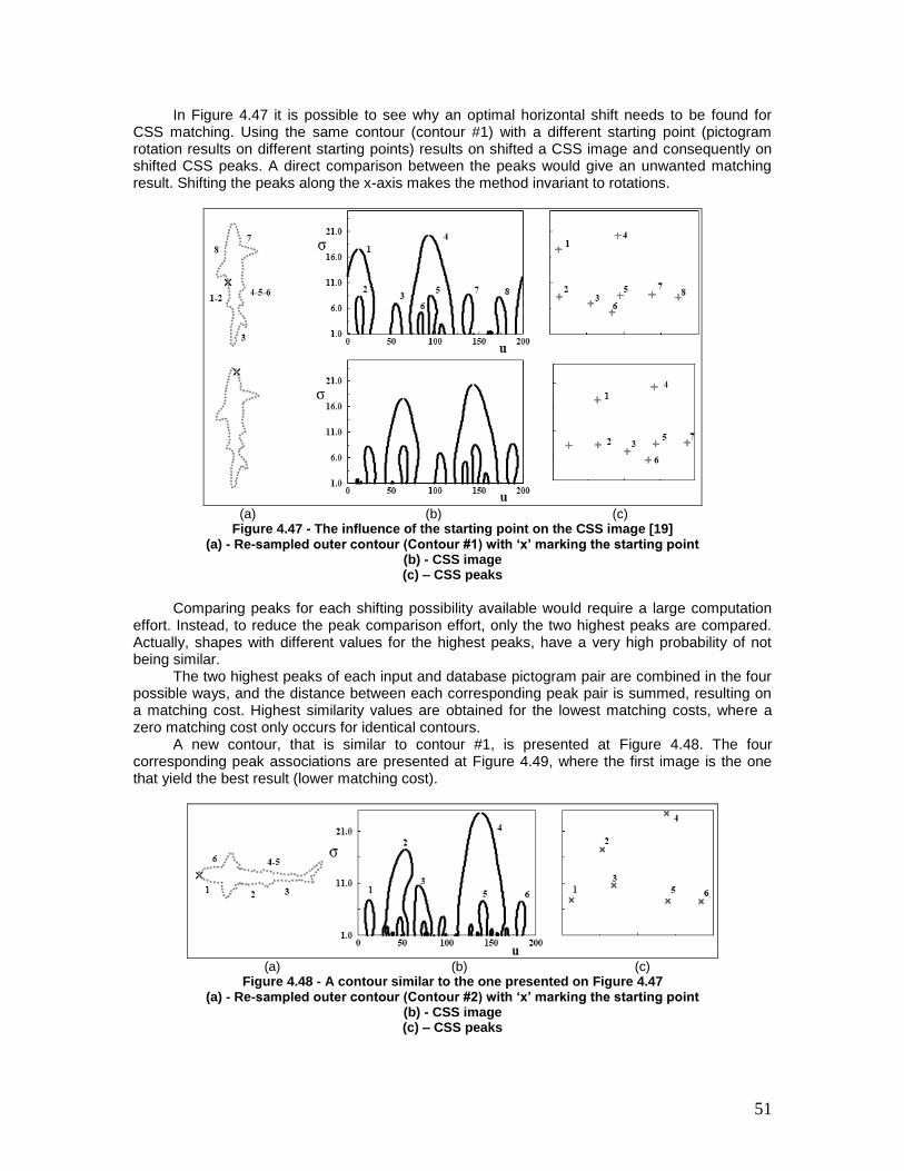
51
In Figure 4.47 it is possible to see why an optimal horizontal shift needs to be found for CSS matching. Using the same contour (contour #1) with a different starting point (pictogram rotation results on different starting points) results on shifted a CSS image and consequently on shifted CSS peaks. A direct comparison between the peaks would give an unwanted matching result. Shifting the peaks along the x-axis makes the method invariant to rotations.
(a) (b) (c)
Figure 4.47 - The influence of the starting point on the CSS image [19] (a) - Re-sampled outer contour (Contour #1) with „x‟ marking the starting point
(b) - CSS image (c) – CSS peaks
Comparing peaks for each shifting possibility available would require a large computation
effort. Instead, to reduce the peak comparison effort, only the two highest peaks are compared. Actually, shapes with different values for the highest peaks, have a very high probability of not being similar.
The two highest peaks of each input and database pictogram pair are combined in the four possible ways, and the distance between each corresponding peak pair is summed, resulting on a matching cost. Highest similarity values are obtained for the lowest matching costs, where a zero matching cost only occurs for identical contours.
A new contour, that is similar to contour #1, is presented at Figure 4.48. The four corresponding peak associations are presented at Figure 4.49, where the first image is the one that yield the best result (lower matching cost).
(a) (b) (c)
Figure 4.48 - A contour similar to the one presented on Figure 4.47 (a) - Re-sampled outer contour (Contour #2) with „x‟ marking the starting point
(b) - CSS image (c) – CSS peaks
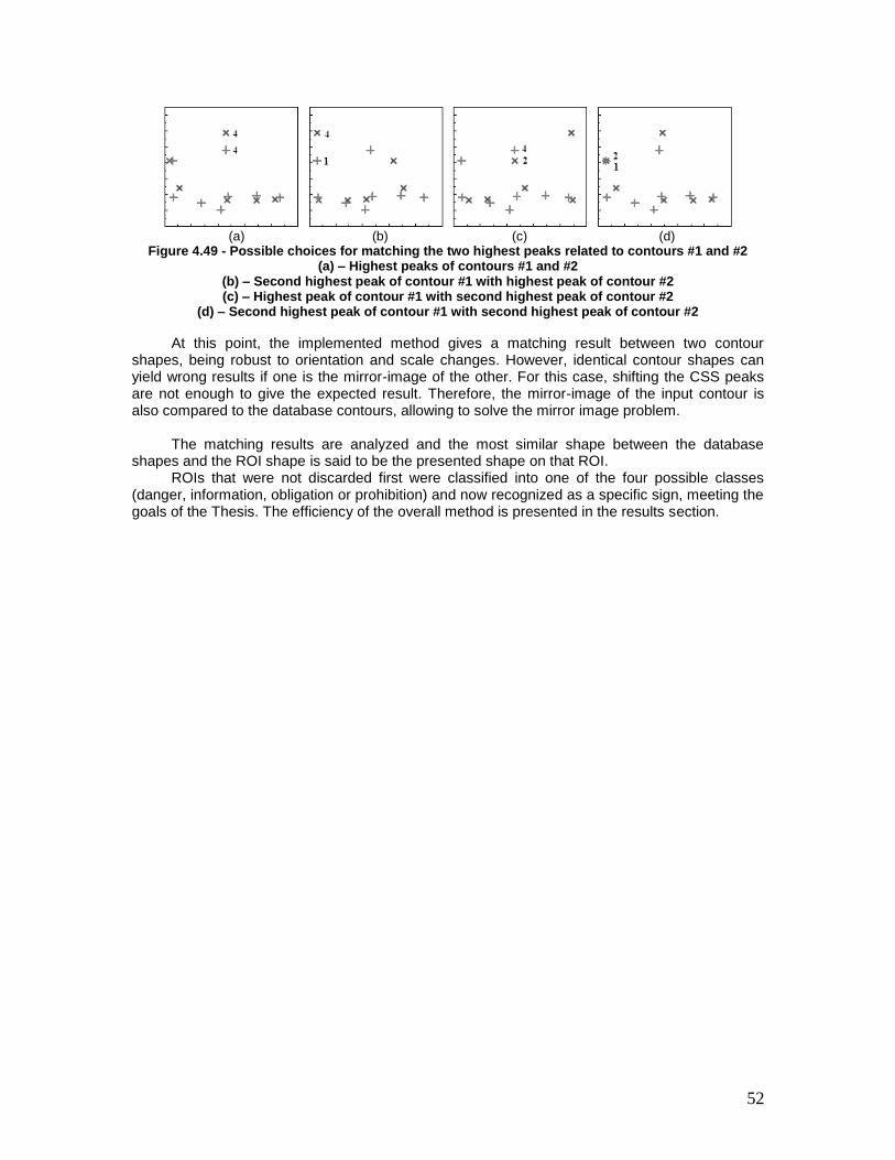
52
(a) (b) (c) (d)
Figure 4.49 - Possible choices for matching the two highest peaks related to contours #1 and #2 (a) – Highest peaks of contours #1 and #2
(b) – Second highest peak of contour #1 with highest peak of contour #2 (c) – Highest peak of contour #1 with second highest peak of contour #2
(d) – Second highest peak of contour #1 with second highest peak of contour #2
At this point, the implemented method gives a matching result between two contour shapes, being robust to orientation and scale changes. However, identical contour shapes can yield wrong results if one is the mirror-image of the other. For this case, shifting the CSS peaks are not enough to give the expected result. Therefore, the mirror-image of the input contour is also compared to the database contours, allowing to solve the mirror image problem.
The matching results are analyzed and the most similar shape between the database
shapes and the ROI shape is said to be the presented shape on that ROI. ROIs that were not discarded first were classified into one of the four possible classes
(danger, information, obligation or prohibition) and now recognized as a specific sign, meeting the goals of the Thesis. The efficiency of the overall method is presented in the results section.
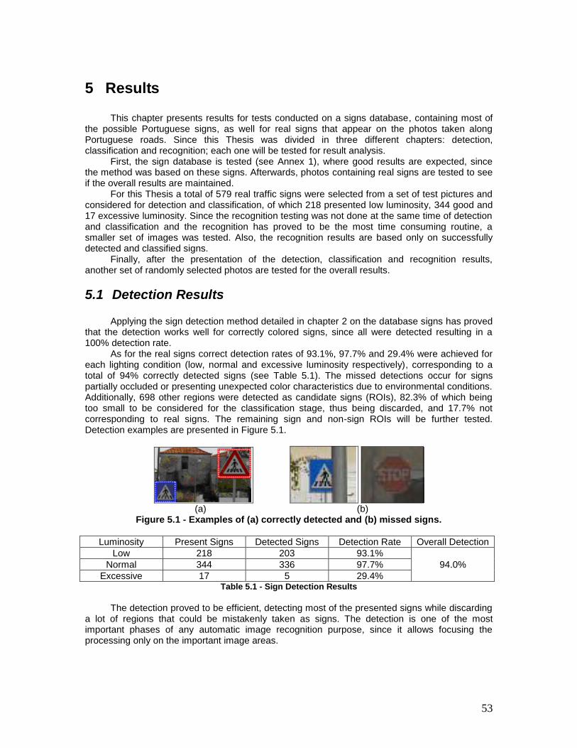
53
5 Results
This chapter presents results for tests conducted on a signs database, containing most of the possible Portuguese signs, as well for real signs that appear on the photos taken along Portuguese roads. Since this Thesis was divided in three different chapters: detection, classification and recognition; each one will be tested for result analysis.
First, the sign database is tested (see Annex 1), where good results are expected, since the method was based on these signs. Afterwards, photos containing real signs are tested to see if the overall results are maintained.
For this Thesis a total of 579 real traffic signs were selected from a set of test pictures and considered for detection and classification, of which 218 presented low luminosity, 344 good and 17 excessive luminosity. Since the recognition testing was not done at the same time of detection and classification and the recognition has proved to be the most time consuming routine, a smaller set of images was tested. Also, the recognition results are based only on successfully detected and classified signs.
Finally, after the presentation of the detection, classification and recognition results, another set of randomly selected photos are tested for the overall results.
5.1 Detection Results Applying the sign detection method detailed in chapter 2 on the database signs has proved
that the detection works well for correctly colored signs, since all were detected resulting in a 100% detection rate.
As for the real signs correct detection rates of 93.1%, 97.7% and 29.4% were achieved for each lighting condition (low, normal and excessive luminosity respectively), corresponding to a total of 94% correctly detected signs (see Table 5.1). The missed detections occur for signs partially occluded or presenting unexpected color characteristics due to environmental conditions. Additionally, 698 other regions were detected as candidate signs (ROIs), 82.3% of which being too small to be considered for the classification stage, thus being discarded, and 17.7% not corresponding to real signs. The remaining sign and non-sign ROIs will be further tested. Detection examples are presented in Figure 5.1.
(a) (b)
Figure 5.1 - Examples of (a) correctly detected and (b) missed signs.
Luminosity Present Signs Detected Signs Detection Rate Overall Detection
Low 218 203 93.1%
94.0% Normal 344 336 97.7%
Excessive 17 5 29.4% Table 5.1 - Sign Detection Results
The detection proved to be efficient, detecting most of the presented signs while discarding
a lot of regions that could be mistakenly taken as signs. The detection is one of the most important phases of any automatic image recognition purpose, since it allows focusing the processing only on the important image areas.
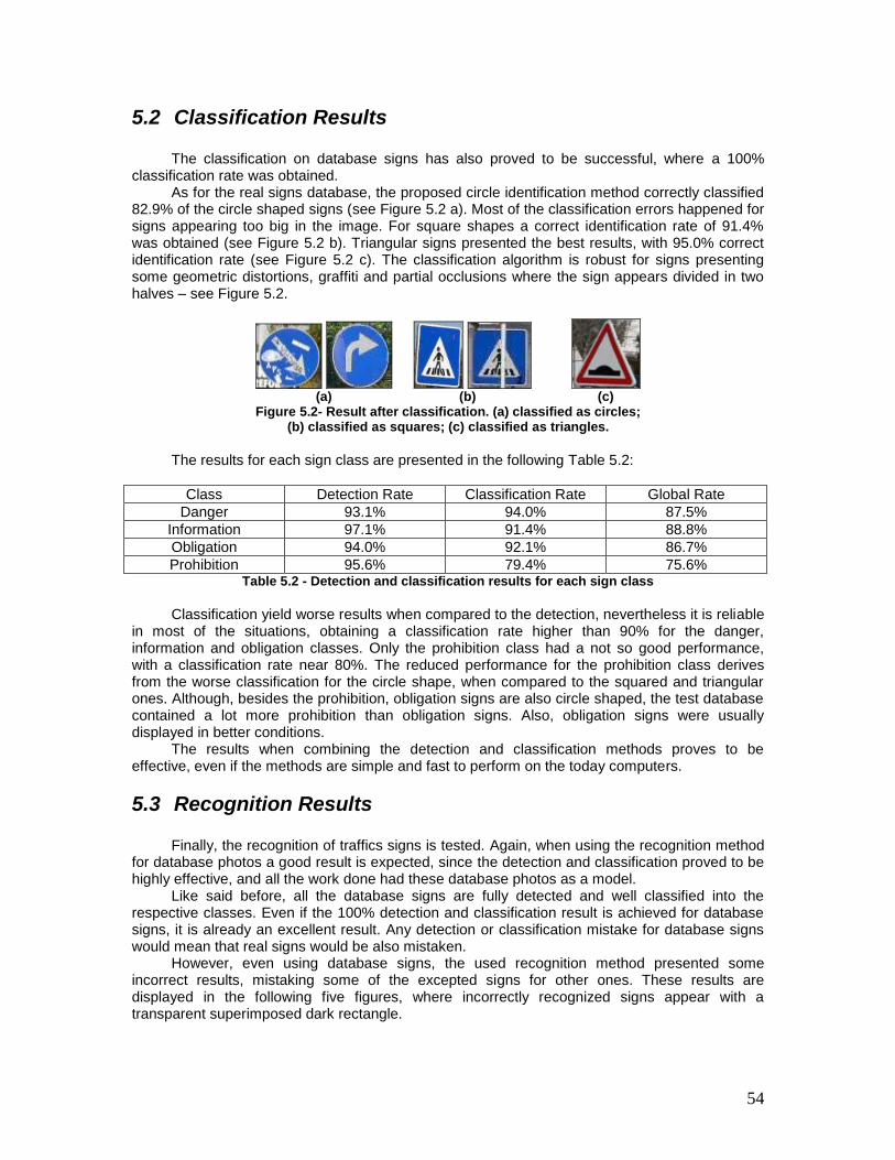
54
5.2 Classification Results The classification on database signs has also proved to be successful, where a 100%
classification rate was obtained. As for the real signs database, the proposed circle identification method correctly classified
82.9% of the circle shaped signs (see Figure 5.2 a). Most of the classification errors happened for signs appearing too big in the image. For square shapes a correct identification rate of 91.4% was obtained (see Figure 5.2 b). Triangular signs presented the best results, with 95.0% correct identification rate (see Figure 5.2 c). The classification algorithm is robust for signs presenting some geometric distortions, graffiti and partial occlusions where the sign appears divided in two halves – see Figure 5.2.
(a) (b) (c)
Figure 5.2- Result after classification. (a) classified as circles; (b) classified as squares; (c) classified as triangles.
The results for each sign class are presented in the following Table 5.2:
Class Detection Rate Classification Rate Global Rate
Danger 93.1% 94.0% 87.5%
Information 97.1% 91.4% 88.8%
Obligation 94.0% 92.1% 86.7%
Prohibition 95.6% 79.4% 75.6% Table 5.2 - Detection and classification results for each sign class
Classification yield worse results when compared to the detection, nevertheless it is reliable
in most of the situations, obtaining a classification rate higher than 90% for the danger, information and obligation classes. Only the prohibition class had a not so good performance, with a classification rate near 80%. The reduced performance for the prohibition class derives from the worse classification for the circle shape, when compared to the squared and triangular ones. Although, besides the prohibition, obligation signs are also circle shaped, the test database contained a lot more prohibition than obligation signs. Also, obligation signs were usually displayed in better conditions.
The results when combining the detection and classification methods proves to be effective, even if the methods are simple and fast to perform on the today computers.
5.3 Recognition Results Finally, the recognition of traffics signs is tested. Again, when using the recognition method
for database photos a good result is expected, since the detection and classification proved to be highly effective, and all the work done had these database photos as a model.
Like said before, all the database signs are fully detected and well classified into the respective classes. Even if the 100% detection and classification result is achieved for database signs, it is already an excellent result. Any detection or classification mistake for database signs would mean that real signs would be also mistaken.
However, even using database signs, the used recognition method presented some incorrect results, mistaking some of the excepted signs for other ones. These results are displayed in the following five figures, where incorrectly recognized signs appear with a transparent superimposed dark rectangle.
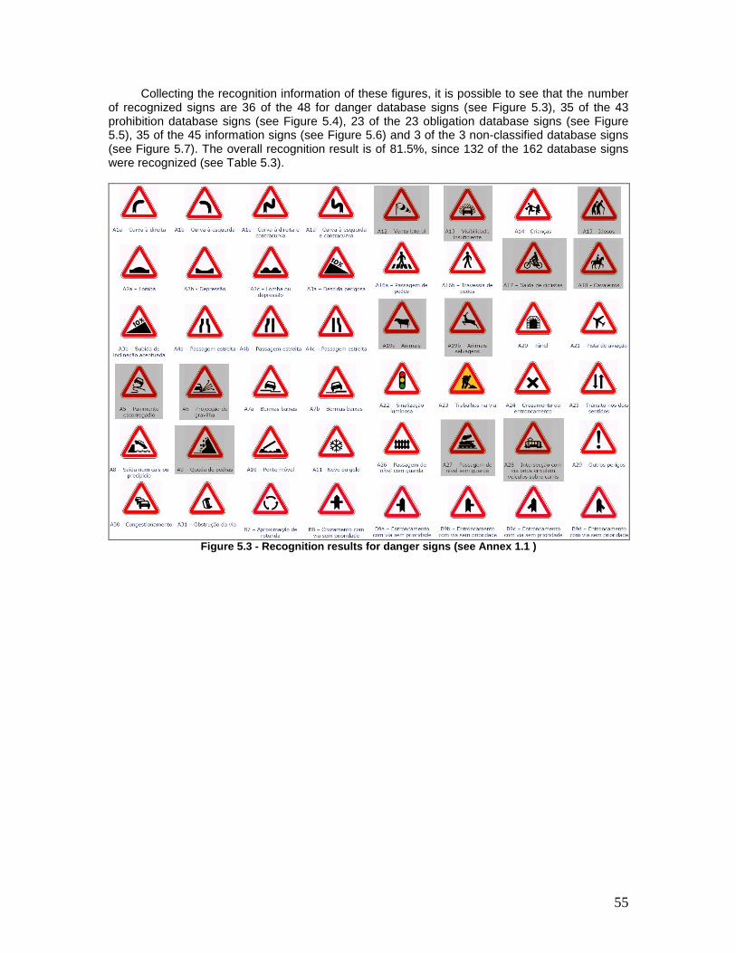
55
Collecting the recognition information of these figures, it is possible to see that the number of recognized signs are 36 of the 48 for danger database signs (see Figure 5.3), 35 of the 43 prohibition database signs (see Figure 5.4), 23 of the 23 obligation database signs (see Figure 5.5), 35 of the 45 information signs (see Figure 5.6) and 3 of the 3 non-classified database signs (see Figure 5.7). The overall recognition result is of 81.5%, since 132 of the 162 database signs were recognized (see Table 5.3).
Figure 5.3 - Recognition results for danger signs (see Annex 1.1 )
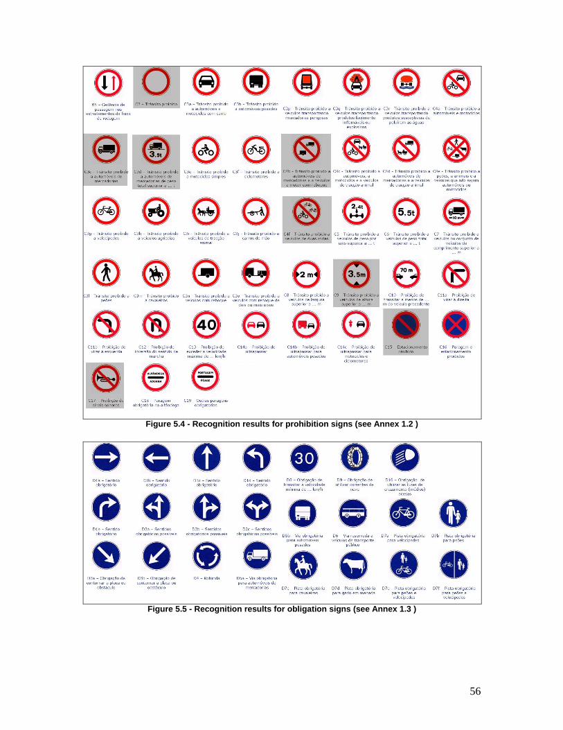
56
Figure 5.4 - Recognition results for prohibition signs (see Annex 1.2 )
Figure 5.5 - Recognition results for obligation signs (see Annex 1.3 )
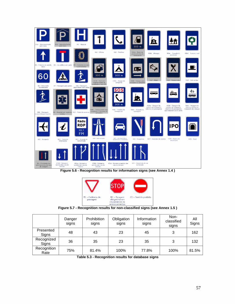
57
Figure 5.6 - Recognition results for information signs (see Annex 1.4 )
Figure 5.7 - Recognition results for non-classified signs (see Annex 1.5 )
Danger signs
Prohibition signs
Obligation signs
Information signs
Non-classified
signs
All Signs
Presented Signs
48 43 23 45 3 162
Recognized Signs
36 35 23 35 3 132
Recognition Rate
75% 81.4% 100% 77.8% 100% 81.5%
Table 5.3 - Recognition results for database signs
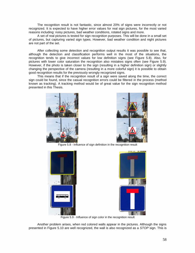
58
The recognition result is not fantastic, since almost 20% of signs were incorrectly or not recognized. It is expected to have higher error values for real sign pictures, for the most varied reasons including: noisy pictures, bad weather conditions, rotated signs and more.
A set of real pictures is tested for sign recognition purposes. This will be done in a small set of pictures, but capturing varied sign types. However, bad weather condition and night pictures are not part of the set.
After collecting some detection and recognition output results it was possible to see that,
although the detection and classification performs well in the most of the situations, the recognition tends to give incorrect values for low definition signs (see Figure 5.8). Also, for pictures with lower color saturation the recognition also mistakes signs often (see Figure 5.9). However, if the photo is taken closer to the sign (resulting in a higher definition sign) or slightly changing the perspective of the camera (resulting in a more colorful sign) it is possible to obtain good recognition results for the previously wrongly recognized signs.
This means that if the recognition result of a sign were saved along the time, the correct sign could be found, since the casual recognition errors could be filtered in the process (method known as tracking). A tracking method would be of great value for the sign recognition method presented in this Thesis.
Figure 5.8 - Influence of sign definition in the recognition result
Figure 5.9 - Influence of sign color in the recognition result
Another problem arises, when red colored walls appear in the pictures. Although the signs
presented in Figure 5.10 are well recognized, the wall is also recognized as a STOP sign. This is
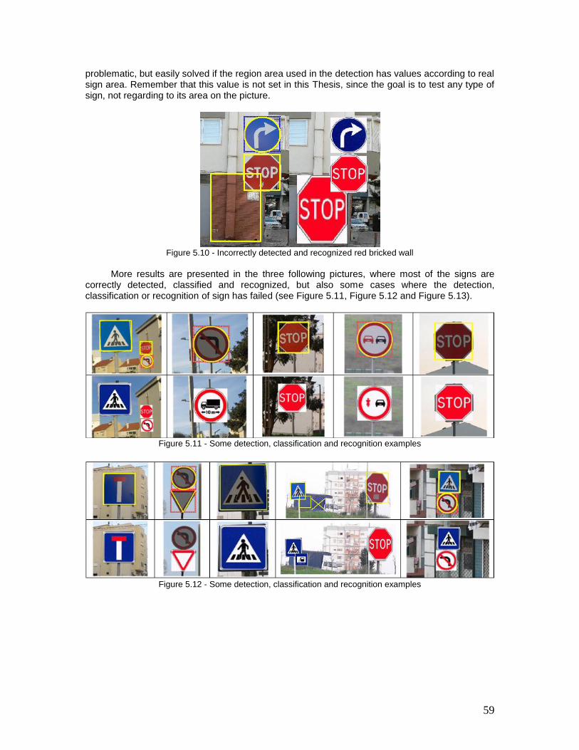
59
problematic, but easily solved if the region area used in the detection has values according to real sign area. Remember that this value is not set in this Thesis, since the goal is to test any type of sign, not regarding to its area on the picture.
Figure 5.10 - Incorrectly detected and recognized red bricked wall
More results are presented in the three following pictures, where most of the signs are
correctly detected, classified and recognized, but also some cases where the detection, classification or recognition of sign has failed (see Figure 5.11, Figure 5.12 and Figure 5.13).
Figure 5.11 - Some detection, classification and recognition examples
Figure 5.12 - Some detection, classification and recognition examples
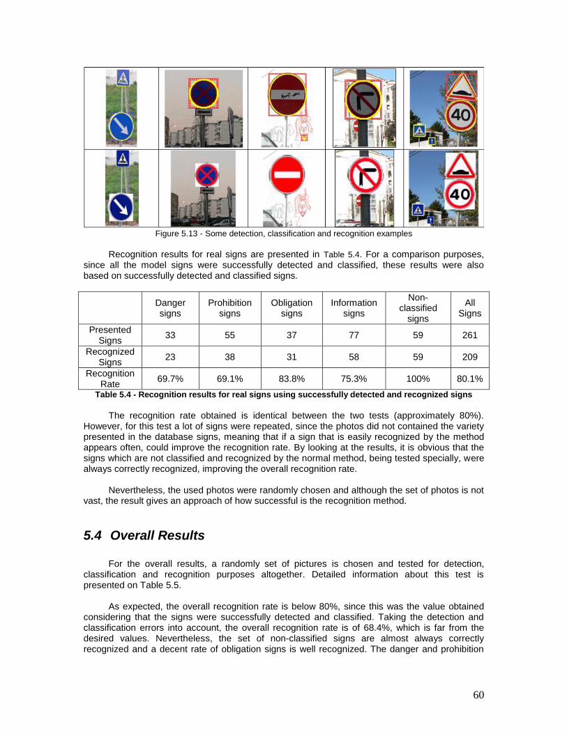
60
Figure 5.13 - Some detection, classification and recognition examples
Recognition results for real signs are presented in Table 5.4. For a comparison purposes,
since all the model signs were successfully detected and classified, these results were also based on successfully detected and classified signs.
Danger signs
Prohibition signs
Obligation signs
Information signs
Non-classified
signs
All Signs
Presented Signs
33 55 37 77 59 261
Recognized Signs
23 38 31 58 59 209
Recognition Rate
69.7% 69.1% 83.8% 75.3% 100% 80.1%
Table 5.4 - Recognition results for real signs using successfully detected and recognized signs
The recognition rate obtained is identical between the two tests (approximately 80%).
However, for this test a lot of signs were repeated, since the photos did not contained the variety presented in the database signs, meaning that if a sign that is easily recognized by the method appears often, could improve the recognition rate. By looking at the results, it is obvious that the signs which are not classified and recognized by the normal method, being tested specially, were always correctly recognized, improving the overall recognition rate.
Nevertheless, the used photos were randomly chosen and although the set of photos is not
vast, the result gives an approach of how successful is the recognition method.
5.4 Overall Results
For the overall results, a randomly set of pictures is chosen and tested for detection,
classification and recognition purposes altogether. Detailed information about this test is presented on Table 5.5.
As expected, the overall recognition rate is below 80%, since this was the value obtained
considering that the signs were successfully detected and classified. Taking the detection and classification errors into account, the overall recognition rate is of 68.4%, which is far from the desired values. Nevertheless, the set of non-classified signs are almost always correctly recognized and a decent rate of obligation signs is well recognized. The danger and prohibition
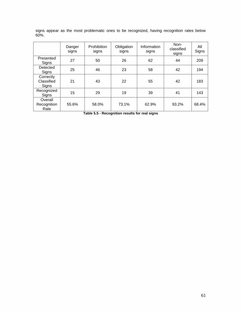
61
signs appear as the most problematic ones to be recognized, having recognition rates below 60%.
Danger signs
Prohibition signs
Obligation signs
Information signs
Non-classified
signs
All Signs
Presented Signs
27 50 26 62 44 209
Detected Signs
25 46 23 58 42 194
Correctly Classified
Signs 21 43 22 55 42 183
Recognized Signs
15 29 19 39 41 143
Overall Recognition
Rate 55.6% 58.0% 73.1% 62.9% 93.2% 68.4%
Table 5.5 - Recognition results for real signs
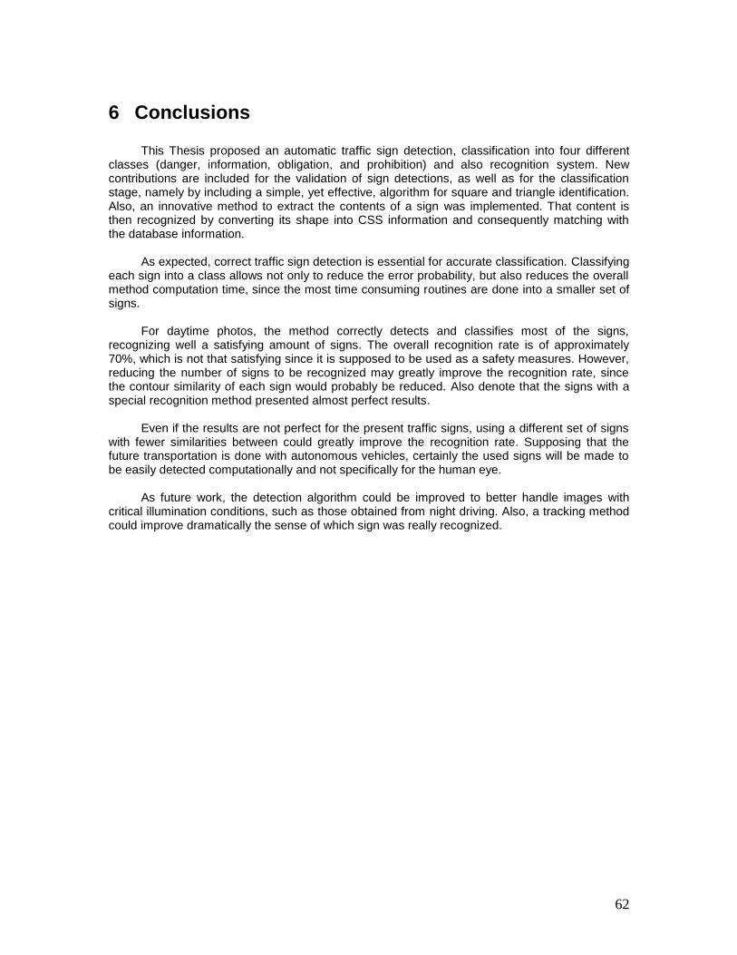
62
6 Conclusions
This Thesis proposed an automatic traffic sign detection, classification into four different classes (danger, information, obligation, and prohibition) and also recognition system. New contributions are included for the validation of sign detections, as well as for the classification stage, namely by including a simple, yet effective, algorithm for square and triangle identification. Also, an innovative method to extract the contents of a sign was implemented. That content is then recognized by converting its shape into CSS information and consequently matching with the database information.
As expected, correct traffic sign detection is essential for accurate classification. Classifying
each sign into a class allows not only to reduce the error probability, but also reduces the overall method computation time, since the most time consuming routines are done into a smaller set of signs.
For daytime photos, the method correctly detects and classifies most of the signs,
recognizing well a satisfying amount of signs. The overall recognition rate is of approximately 70%, which is not that satisfying since it is supposed to be used as a safety measures. However, reducing the number of signs to be recognized may greatly improve the recognition rate, since the contour similarity of each sign would probably be reduced. Also denote that the signs with a special recognition method presented almost perfect results.
Even if the results are not perfect for the present traffic signs, using a different set of signs
with fewer similarities between could greatly improve the recognition rate. Supposing that the future transportation is done with autonomous vehicles, certainly the used signs will be made to be easily detected computationally and not specifically for the human eye.
As future work, the detection algorithm could be improved to better handle images with
critical illumination conditions, such as those obtained from night driving. Also, a tracking method could improve dramatically the sense of which sign was really recognized.
63
References
[1] C. Bahlmann, Y. Zhu, V. Ramesh, M. Pellkofer, T. Koehler, “A system for traffic sign detection, tracking and recognition using color, shape, and motion information”, Proceedings of the Intelligent Vehicles Symposium, IEEE, pp. 255-260, June 2005 [2] S. Estable, J. Schick, F. Stein, R. Ott, R. Janssen, W. Ritter, and Y.J. Zheng, “A Real-Time Traffic Sign Recognition Systems”, Proceedings of the Intelligent Vehicles ’94 Symposium, IEEE, pp. 24-26, October 1994 [3] G.K. Siogkas, and E.S. Dermatas, “Detection, Tracking and Classification of Road Signs in Adverse Conditions”, MELECON 2006, pp. 537-540, May 2006 [4] X.W. Gao, L. Podladchikova, D. Shaposhnikov, K. Hong, and N. Shevtsova, “Recognition of traffic signs based on their colour and shape features extracted using human vision models”, Journal of Visual Communication and Image Representation, October 2005 [5] A. de la Escalera, L.E. Moreno, M.A. Salichs, and J.M. Armingol, “Traffic Sign Detection for Driver Support Systems”, International Conference on Field and Service Robotics, Espoo, Finland, June 2001 [6] A. de la Escalera, L.E. Moreno, M.A. Salichs, and J.M. Armingol, “Road Traffic Sign Detection and Classification”, IEEE Transactions on Industrial Electronics, vol. 44, nº 6, pp. 848-859, December 1997 [7] C.-Y. Fang, S.-W. Chen, and C.-S. Fuh, “Road-sign detection and tracking”, IEEE transactions on vehicular technology, vol. 52, nº 5, pp. 1329-1341, September 2003 [8] C. Harris and M.J. Stephens, “A combined corner and edge detector”, Alvey Vision Conference, pp 147-152, 1988 [9] G. Loy, and A. Zelinsky, “Fast Radial Symmetry for Detecting Points of Interest”, IEEE Transactions on Pattern Analysis and Machine Intelligence, vol. 25, nº 8, pp 959-973, August 2003 [10] N. Otsu, “A threshold selection method from gray-level histogram”, IEEE Transactions on System Man Cybernetics, vol. SMC-9, nº 1, pp 62-66, April 1994 [11] “Active Contours, Deformable Models, and Gradient Vector Flow”, http://iacl.ece.jhu.edu/projects/gvf/ [12] Stella Atkins, SFU Medical and Image Computing Analysis (MICA) Lab, Simon Fraser University, http://www.cs.sfu.ca/~stella/papers/blairthesis/main/node31.html [13] Chenyang Xu and Jerry L. Prince, “Gradient Vector Flow: A New External Force for Snakes”, Department of Electrical and Computer Engineering, The Johns Hopkins University, Baltimore, MD 21218 [14] Farzin Mokhtarian, “Silhouette-Based Isolated Object Recognition through Curvature Scale Space”, IEEE Transactions on Pattern Analysis and Machine Intelligence, vol. 17, nº 5, May 1995 [15] Farzin Mokhtarian, Sadegh Abbasi and Josef Kittler, “Robust and Efficient Shape Indexing through Curvature Scale Space”, Department of Electronic & Electrical Engineering, University of Surrey, England [16] Farzin Mokhtarian and Alan K. Mackworth, “A Theory of Multiscale, Curvature-Based Shape Representation for Planar Curves”, IEEE Transactions on Pattern Analysis and Machine Intelligence, vol. 14, nº8, August 1992 [17] Carla Zibreira, “Descrição e Procura de Vídeo Baseadas na Forma”, Instituto Superior Técnico, Technical University of Lisbon, Portugal, 2000 [18] B. S. Manjunath, Philippe Salembier, Thomas Sikora, “Introduction to MPEG-7: Multimedia Content Description Interface”, ISBN: 978-0-471-48678-7, Hardcover, 396 pages, April 2002 [19] Farzin Mokhtarian, Sadegh Abbasi and Josef Kittler, “Efficient and Robust Retrieval by Shape Content Through Curvature Scale Space”, Proceedings of International Workshop on Image Databases and Multimedia Search, pp 35-42, Amsterdam, The Netherlands, 1996 [WIAMIS] Carlos Paulo, Paulo Correia, “Automatic Detection and Classification of Traffic Signs”, Instituto Superior Técnico, Technical University of Lisbon, Portugal, 2007
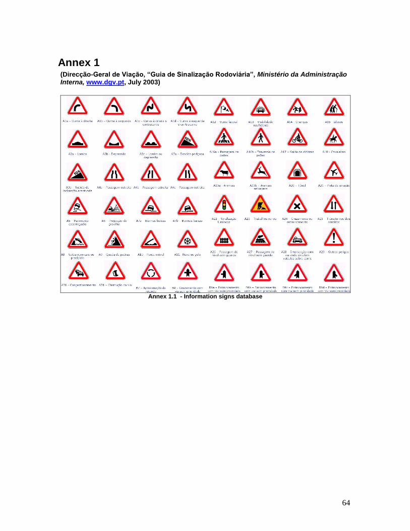
64
Annex 1 (Direcção-Geral de Viação, “Guia de Sinalização Rodoviária”, Ministério da Administração Interna, www.dgv.pt, July 2003)
Annex 1.1 - Information signs database
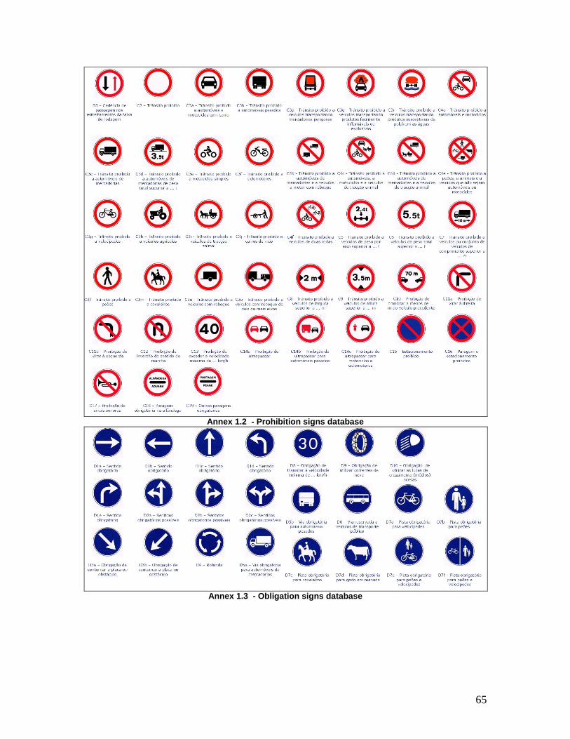
65
Annex 1.2 - Prohibition signs database
Annex 1.3 - Obligation signs database
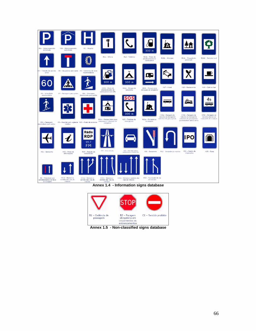
66
Annex 1.4 - Information signs database
Annex 1.5 - Non-classified signs database
67
Annex 2
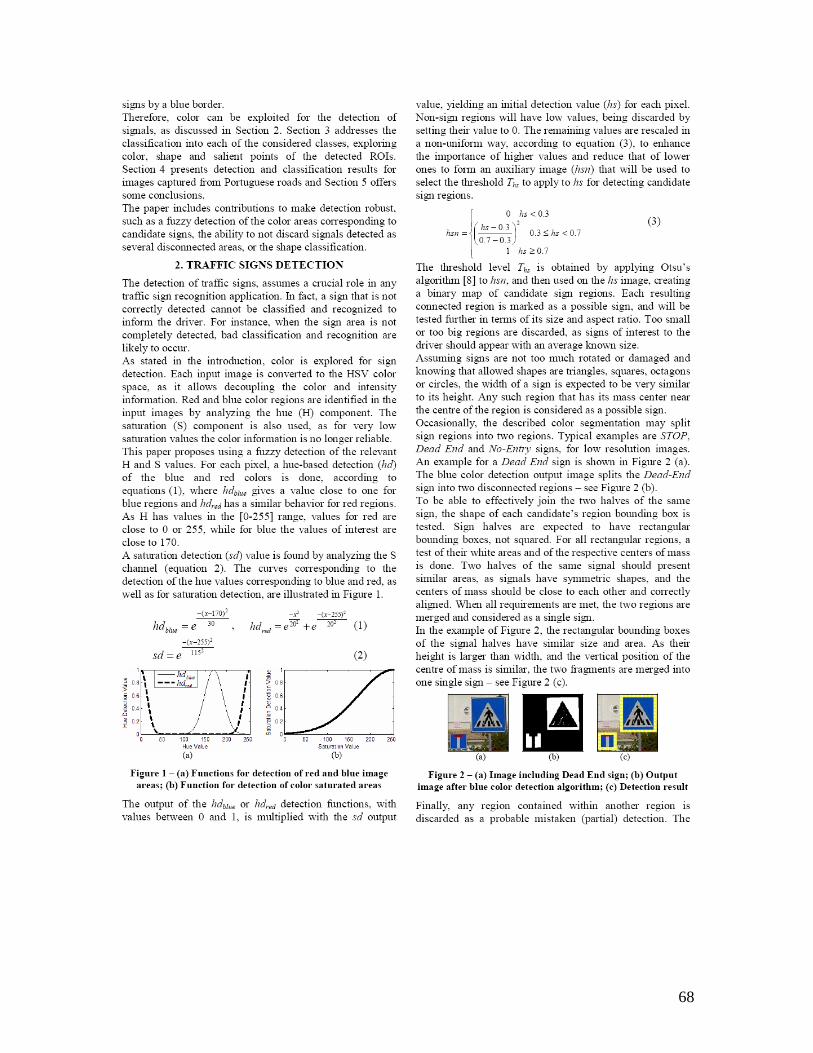
68
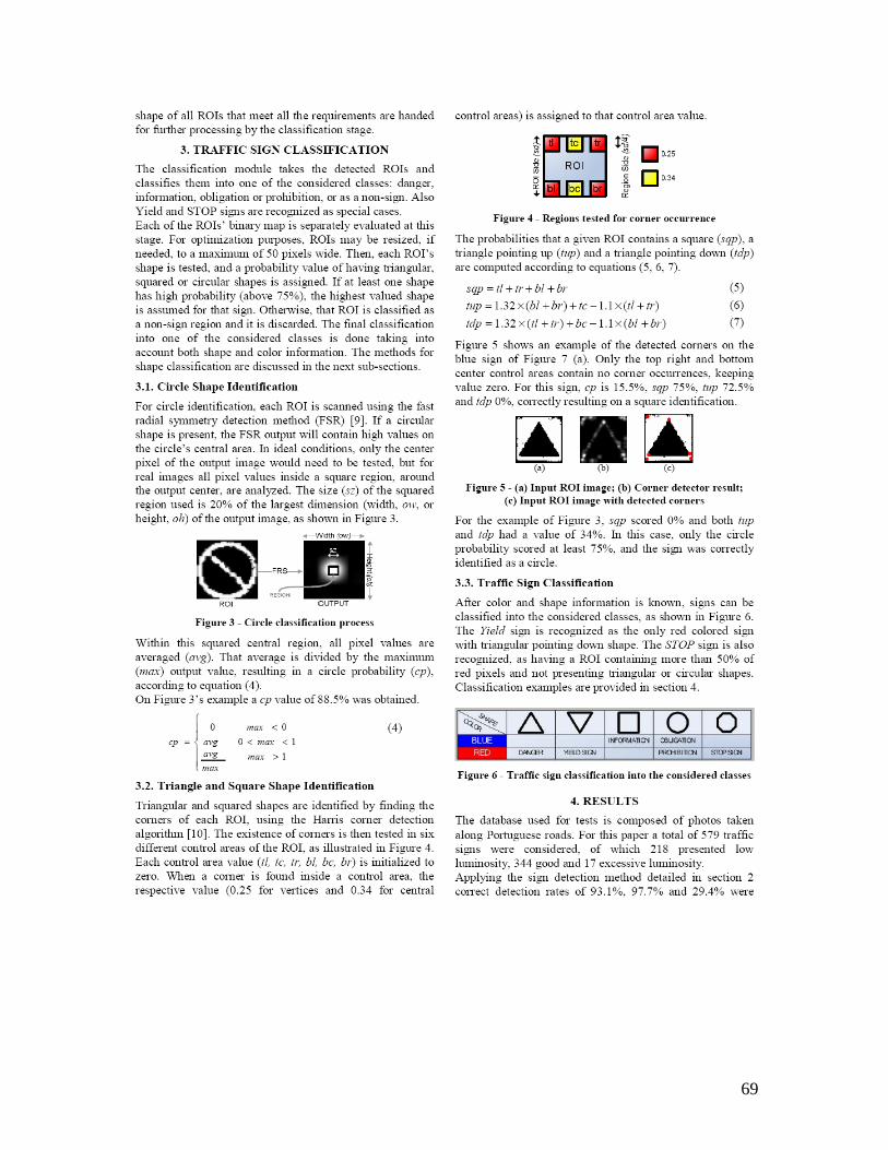
69
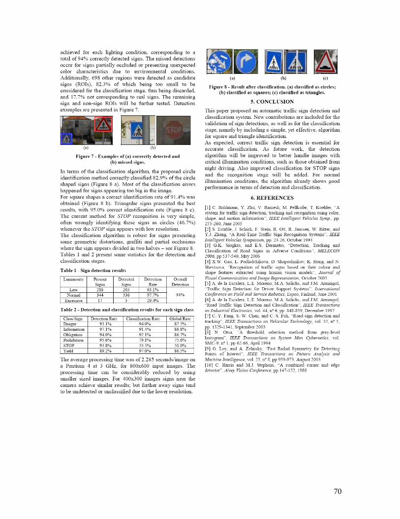
70