DETECTION AND CLASSIFICATION OF POLE-LIKE OBJECTS …

DETECTION AND CLASSIFICATION OF POLE-LIKE OBJECTS

FROM MOBILE MAPPING DATA

K. Fukano a , H. Masuda a, *

a Dept. of Mechanical Engineering and Intelligent Systems, The University of Electro-Communications,

1-5-1 Chofugaoka, Chofu, Tokyo, Japan - (kenta.fukano, h.masuda)@uec.ac.jp

Commission V, ICWG I/Va

KEY WORDS: Mobile Mapping System, classification, point-cloud, recognition, roadside objects, machine learning

ABSTRACT:

Laser scanners on a vehicle-based mobile mapping system can capture 3D point-clouds of roads and roadside objects. Since roadside

objects have to be maintained periodically, their 3D models are useful for planning maintenance tasks. In our previous work, we

proposed a method for detecting cylindrical poles and planar plates in a point-cloud. However, it is often required to further classify

pole-like objects into utility poles, streetlights, traffic signals and signs, which are managed by different organizations. In addition, our

previous method may fail to extract low pole-like objects, which are often observed in urban residential areas. In this paper, we propose

new methods for extracting and classifying pole-like objects. In our method, we robustly extract a wide variety of poles by converting

point-clouds into wireframe models and calculating cross-sections between wireframe models and horizontal cutting planes. For

classifying pole-like objects, we subdivide a pole-like object into five subsets by extracting poles and planes, and calculate feature

values of each subset. Then we apply a supervised machine learning method using feature variables of subsets. In our experiments, our

method could achieve excellent results for detection and classification of pole-like objects.

1. INTRODUCTION

Laser scanners on a vehicle-based mobile mapping system

(MMS) can capture 3D point-clouds of roads and roadside

objects while running on the road. Roadside objects, such as

utility poles, traffic signs, and streetlights, have to be maintained

periodically. Since there are a huge number of roadside objects

in residential areas, their periodic maintenance tasks are very

costly and time-consuming. If 3D digital data of roadside objects

can be efficiently captured using a MMS, the current statuses of

roadside objects will be easily investigated.

In our previous research, we proposed a method for reliably

detecting cylindrical poles and planar plates from noisy point-

clouds captured by a MMS (Masuda et al., 2013). We projected

points on a horizontal plane and extracted high-density regions.

As shown in Figure 1, the projection of pole-like objects

produces high-density regions, and therefore, the search regions

for pole-like objects can be restricted only in high-density regions.

It is often required to further classify pole-like objects into utility

poles, streetlights, traffic signals, traffic signs, and so on, as

shown in Figure 2. Since streetlights, traffic signals, and utility

poles are managed by different organizations, their classification

is very important for asset management and maintenance.

Identification of object classes is also required for shape

reconstruction, because knowledge-based methods are typical for

reconstructing 3D shapes from incomplete point-clouds (Nan et

al., 2010; Nan et al., 2012; Kim et al., 2012; Lin et al., 2013).

Some researchers studied shape classification for pole-like

objects (Yokoyama et al., 2011; Cabo et al., 2014; Yang et al.,

2015; Kamal et al., 2013; Pu et al, 2011; Li and Oude Elberink,

2013). Their methods are based on threshold values of feature

values, which have to be carefully determined by experiments.

For identifying new object classes, new thresholds have to be

* Corresponding author

investigated. Other researchers introduced supervised machine

learning methods for classifying pole-like objects (Golovinsky et

al., 2009; Zhu et al., 2010; Puttonen et al., 2011; Ishikawa et al.,

2012; Lai and Fox, 2009; Munoz et al, 2009; Oude Elberink and

Kemboi, 2014; Weinmann et al, 2014). In machine learning,

threshold values for classification are automatically determined

based on training data. However, their recognition rates were not

high and the numbers of classes were very limited, because pole-

like objects have similar shapes and therefore they have similar

feature values.

Figure 1. Extraction of high-density regions

Figure 2. Classification of pole-like objects

ISPRS Annals of the Photogrammetry, Remote Sensing and Spatial Information Sciences, Volume II-3/W5, 2015 ISPRS Geospatial Week 2015, 28 Sep – 03 Oct 2015, La Grande Motte, France

This contribution has been peer-reviewed. The double-blind peer-review was conducted on the basis of the full paper. Editors: S. Oude Elberink, A. Velizhev, R. Lindenbergh, S. Kaasalainen, and F. Pirotti

doi:10.5194/isprsannals-II-3-W5-57-2015

57

In this paper, we propose a new method for classifying pole-like

objects into representative classes. In our method, we subdivide

a pole-like object into five subsets by extracting cylinders and

planes. Then we apply a supervised machine learning method to

each subdivided subset. Our approach is very effective for pole-

like objects, because many pole-like objects are characterized

using partial shapes except common poles.

We also consider a new method for detecting pole-like objects.

In our previous work, thin or low poles often fails to be extracted,

because their projected points is not very dense, and therefore, it

is difficult to robustly separate pole parts from what are not poles.

Thin and low poles can be observed mainly in urban residential

areas in Japan.

In this paper, we introduce a section-based method for robustly

detecting pole-like objects. We convert a point-cloud into a

wireframe model and search for a sequence of circular cross-

sections of the wireframe model.

In the following, we describe our new extraction method for pole-

like objects. Then we propose a classification method for pole-

like objects in Section 3. In Section 4, we show experimental

results, and finally we conclude our work in Section 5.

2. EXTRACTION OF POLE-LIKE OBJECTS

2.1 Capturing Point-Clouds of Roadside Objects

A MMS is a vehicle on which laser scanners, GPSs, IMUs, and

cameras are mounted, as shown in Figure 3(a). A laser scanner

emits laser beams to objects while rotating the directions of laser

beams, as shown in Figure 3(b). The rotation frequency of laser

beams is determined by the specification of the laser scanner.

MMS data consist of a sequence of 3D coordinates, which are

optionally combined with GPS time, intensity and colors. GPS

time indicates when each coordinate was captured. Since 3D

coordinates are stored in a file in the order of measurement,

points can be sequentially connected in the order of GPS times,

as shown in Figure 4. In this paper, we call sequentially

connected points as scan lines.

2.2 Rough Segmentation of Scan Lines

When a pole-like object is measured using a laser scanner,

relatively short scan lines are generated. Figure 5 (a) ~ (c) show

scan-lines on a wall, a road, and a pole. Most scan-lines on walls

are long straight lines, and ones on roads are long horizontal lines.

On the other hand, scan lines on poles are circular and relatively

short.

To select scan lines on poles, we apply the principal component

analysis to each scan line and calculate eigenvalues λ1, λ2, and λ3

(λ1 λ2 λ3). We select scan lines as candidates of poles when

λ1 < c1 and λ1 / λ2 < c2 are satisfied. The second condition means

that scan-lines on poles are not straight lines but planar curves.

Figure 6 shows scan-lines that were selected as candidates of

poles. In this example, we used c1 = 50cm and c2 = 100 according

to experiments. The result shows that roads and walls can be

effectively eliminated using the two conditions.

We project selected scan-lines onto a horizontal plane, as shown

in Figure 7(a), and convert points into triangles using the

Delaunay triangulation. We generate edges between points only

when two points are vertices of a triangle and their distance is

shorter than a threshold value. The span of scan-lines can be

estimated as v/f, where v [m/sec] is the average speed of the

vehicle, and f [Hz] is the frequency of the laser scanner. In this

paper, we define the threshold value as kv/f, where k is a constant

value based on the variation of the vehicle speed. In our examples,

we supposed v=11.1 [m/sec] and k=2.5. The value of k was

determined by experiments.

We segment scan-lines connected by the Delaunay triangulation

into the same group. Figure 7(b) shows segmented scan-lines.

(a) Mobile mapping system

(b) Trajectory of laser beams

Figure 3. Laser scanning by a mobile mapping system

Figure 4. Point-cloud and scan-lines

(a) Wall (b) Road (c) Pole

Figure 5. Patterns of scan-lines

Figure 6. Selection of candidate scan-lines




58

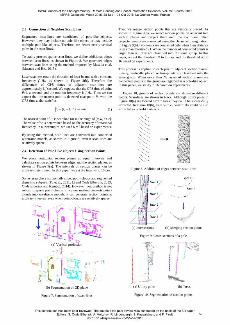
2.3 Connection of Neighbor Scan Lines

Segmented scan-lines are candidates of pole-like objects.

However, they may include no pole-like object, or may include

multiple pole-like objects. Threfore, we detect nearly-vertical

poles in the scan-lines.

To stably process sparse scan-lines, we define additional edges

between scan-lines, as shown in Figure 8. We generated edges

between scan-lines using the method proposed by Masuda et al.

(Masuda and He., 2015).

Laser scanners rotate the direction of laser beams with a constant

frequency f Hz, as shown in Figure 3(b). Therefore the

differences of GPS times of adjacent scan-lines are

approximately 1/f second. We suppose that the GPS time of point

Pi is ti second, and the rotation frequency is f Hz. Then we can

expect that the nearest point is detected near point Pn with the

GPS time tn that satisfies:

min)/1( ftt in (1)

The nearest point of Pi is searched for in the range of [n-w, n+w].

The value of w is determined based on the accuracy of rotational

frequency. In our examples, we used w = 8 based on experiments.

By using this method, scan-lines are converted into connected

wireframe models, as shown in Figure 8, even if scan lines are

relatively sparse.

2.4 Detection of Pole-Like Objects Using Section Points

We place horizontal section planes at equal intervals and

calculate section points between edges and the section planes, as

shown in Figure 9(a). The intervals of section planes can be

arbitrary determined. In this paper, we set the interval to 10 cm.

Some researchers horizontally sliced point-clouds and segmented

them into subparts (Pu et al., 2011; Li and Oude Elberink, 2013;

Oude Elberink and Kemboi, 2014). However their method is not

robust to sparse point-clouds. Since our method converts point-

clouds into wireframe models, it can generate section points at

arbitrary intervals even when point-clouds are relatively sparse.

(a) Vertical projection

(b) Segmentation on 2D plane

Figure 7. Segmentation of scan-lines

Then we merge section points that are vertically placed. As

shown in Figure 9(b), we select section points on adjacent two

section planes and project them onto the x-y plane. Then

projected points are connected using the Delaunay triangulation.

In Figure 9(b), two points are connected only when their distance

is less than threshold D. When the number of connected points is

larger than N1, they are classified into the same group. In this

paper, we set the threshold D to 10 cm, and the threshold N1 to

16 based on experiments.

This process is applied to each pair of adjacent section planes.

Finally, vertically placed section-points are classified into the

same group. When more than N2 layers of section planes are

connected, points in the group are regarded as a pole-like object.

In this paper, we set N2 to 16 based on experiments.

In Figure 10, groups of section points are shown in different

colors. Scan-lines are shown in black. Although utility poles in

Figure 10(a) are located next to trees, they could be successfully

extracted. In Figure 10(b), trees with curved trunks could be also

extracted as pole-like objects.

Figure 8. Addition of edges between scan-lines

(a) Intersections (b) Merging section points

Figure 9. Cross-sections of a pole

(a) Utility poles (b) Trees

Figure 10. Segmentation of section points




59

We can extract original points using section points in the same

group. We suppose that a pole-like object includes section points

P={pi}, and P are generated as the intersection of edges E={ei}.

Then the both end vertices of E are selected as original points on

a pole-like object. Figure 11 shows original points extracted

using section points in Figure 10.

Then we detect additional objects that are attached to poles.

When points on poles are eliminated from segmented scan lines

shown in Figure 7(b), each segment is subdivided into some

connected components. Since attachments of poles are placed at

high positions, components at low positions are discarded. Each

connected component is added to the nearest pole. Figure 12

shows examples of detected pole-like objects. In this figure,

additional components are shown in magenta, and pole-like

objects with attachments are shown in dashed lines.

In this section, we explained the method to extract points on each

pole-like object. In the next section, we discuss how pole-like

objects are classified into utility poles, streetlights, traffic signs,

and so on.

3. CLASSIFICATION OF POLE-LIKE OBJECTS

3.1 Classes of Pole-Like Objects

Pole-like objects include various classes of objects. Since it is

tedious work to manually identify classes of a huge number of

pole-like objects, it is strongly required to automatically classify

pole-like objects. Figure 13 shows examples of pole-like objects,

which include utility poles, traffic signals, traffic signs, direction

boards, streetlights, and trees.

Machine-learning methods are useful for automatically

identifying object classes. In this paper, we consider supervised

machine learning methods, which study the pattern of each class

using labelled training data. In typical methods, each object is

represented using a sequence of values, and a machine learning

system constructs the criteria of classification based on the values.

We describe a sequence of values as a feature vector, and each

variable as a feature variable.

Figure 11. Original points of pole-like objects

Figure 12. Grouping neighbor additional components

Some researchers have proposed classification methods for

point-clouds. Sizes and eigenvalues are often used for

characterizing point-clouds (Golovinsky et al., 2009; Ishikawa et

al., 2012; Yokoyama et al., 2011; Chen et al., 2007; Cabo et al..

2014; Yang et al., 2015). However, conventional feature

variables are not sufficient to distinguish pole-like objects,

because pole-like objects tend to have similar feature values.

Therefore, existing methods could classify pole-like objects into

a single or only a few classes.

To remedy this problem, we subdivide a pole-like object into

several parts by extracting poles and planes. When poles and

planes are extracted and removed from a point-cloud, other parts

can be separated into multiple connected components. Connected

components other than poles give valuable feature variables for

distinguishing pole-like objects.

In this paper, we use the random forest for classifying pole-like

objects (Fukano and Masuda, 2014). The random forest is a

supervised machine learning method, and it is robust to missing

values and outliers in feature values (Breiman, 2001). Since

point-clouds captured by a MMS include a lot of noises and

missing points, the random forest is suitable for our purpose.

(a) Utility pole

(b) Streetlight (c) Highway light

(d) Traffic sign

(e) Direction board

(f) Signal (g) Tree

Figure 13. Pole-like objects on roadsides




60

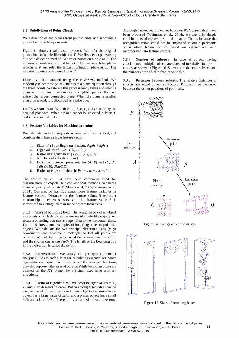
3.2 Subdivision of Point-Clouds

We extract poles and planes from point-clouds, and subdivide a

point-cloud into five point-sets.

Figure 14 shows a subdivision process. We refer the original

point-cloud of a pole-like object as P. We first detect poles using

our pole detection method. We refer points on a pole as A. The

remaining points are referred to as B. Then we search for planar

regions in B and refer the largest continuous plane as C. The

remaining points are referred to as D.

Planes can be extracted using the RANSAC method. We

randomly select three points and create a plane equation through

the three points. We iterate this process many times and select a

plane with the maximum number of neighbor points. Then we

extract the largest connected plane. When the plane is smaller

than a threshold, it is discarded as a false one.

Finally we can obtain five subsets P, A, B, C, and D including the

original point-set. When a plane cannot be detected, subsets C

and D become null sets.

3.3 Feature Variables for Machine Learning

We calculate the following feature variables for each subset, and

combine them into a single feature vector.

1. Sizes of a bounding box: ( width, depth, height )

2. Eigenvalues of PCA: ( λ1, λ2, λ3 )

3. Ratios of eigenvalues: ( λ1/λ2, λ2/λ3, λ1/λ3 )

4. Numbers of subsets: ( num )

5. Distances between point-sets for (A, B) and (C, D):

( dist(A,B), dist(C,D) )

6. Ratios of edge directions in P: ( nh / n, nv / n, na / n )

The feature values 1~4 have been commonly used for

classification of objects, but conventional methods calculated

them only using all points P (Munoz et al, 2009; Weinman et al,

2014). Our method has five times more feature variables in

feature vectors. Distances in the feature values 5 represent

relationships between subsets, and the feature value 6 is

introduced to distinguish man-made objects from trees.

3.3.1 Sizes of bounding box: The bounding box of an object

represents a rough shape. Since we consider pole-like objects, we

create a bounding box that is perpendicular the horizontal plane.

Figure 15 shows some examples of bounding boxes of pole-like

objects. We calculate the two principal directions using (x, y)

coordinates, and generate a rectangle so that all points are

covered. We call the longer edge of the rectangle as the width,

and the shorter one as the depth. The length of the bounding box

in the z direction is called the height.

3.3.2 Eigenvalues: We apply the principal component

analysis (PCA) to each subset for calculating eigenvalues. Since

eigenvalues are equivalent to variances in the principal directions,

they also represent the sizes of objects. While bounding boxes are

defined on the XY plane, the principal axes have arbitrary

directions.

3.3.3 Ratios of Eigenvalues: We describe eigenvalues as λ1,

λ2, and λ3 in descending order. Ratios among eigenvalues can be

used to classify linear objects and planar objects, because a linear

object has a large value of λ1/λ2, and a planar object has a small

λ1/λ2 and a large λ1/λ3. These ratios are added in feature vectors.

Although various feature values based on PCA eigenvalues have

been proposed (Weinman et al., 2014), we use only simple

combinations of eigenvalues in this paper. This is because the

recognition ratios could not be improved in our experiments

when other feature values based on eigenvalues were

incorporated into feature vectors.

3.3.4 Number of subsets: In case of objects having

attachments, multiple subsets are detected in subdivision point-

clouds, as shown in Figure 16. So we count detected subsets, and

the numbers are added to feature variables.

3.3.5 Distances between subsets: The relative distances of

subsets are added to feature vectors. Distances are measured

between the center positions of point-sets.

Figure 14. Five groups of point-sets

Figure 15. Sizes of bounding boxes




61

3.3.6 Ratios of edge directions: A point-cloud is represented

as a wireframe model. Then edges in the wireframe model are

smoothed using the Taubin filter, which is a well-known low-

pass filter for 3D objects (Taubin, 1995). While edges of a tree

have various directions, ones of a man-made object tend to have

horizontal or vertical directions. Figure 17 shows smoothed

edges of a tree and a man-made object. Edges are classified into

three groups based on the angles from the horizontal plane. When

the angle of an edge is less than 30°, it is categorized into the

horizontal group. When the angle is larger than 60°, the edge is

classified into the vertical group. Other edges are categorized into

the angled group. We count the number of edges for each group

and calculate three ratios nh /n, nv /n and na/n, where n is the total

number of points; nh, nv, and na are the numbers of horizontal,

vertical, and angled edges, respectively.

3.4 Classification using Feature Vectors

In the list of feature variables, features 1~4 are calculated for each

of five point-sets; feature 5 is calculated for two pairs (A, B) and

(C, D); feature 6 is calculated only for P. Therefore, we totally

define 55 feature variables, as shown in Table 1.

The number of our feature variables is much larger than ones of

conventional methods. When the random forest is applied to

feature vectors with 55 variables, it automatically constructs

decision trees. If important features are included in variables of

subsets A, B, C, and D, our method can improve recognition

ratios compared to conventional methods, which use only

variables of all points P.

Figure 16. A signal having multiple subsets

Figure 17. Smoothed edges

4. EXPERIMENTAL RESULTS

4.1 Detection of Pole-Like Objects

We extracted poles from point-clouds measured in a residential

district in a Japanese urban city. The number of points was 1.3

hundred millions. A lot of low pole-like objects are included in

this district. In our experiments, we automatically extracted pole-

like objects and displayed them with the whole point-clouds on

the screen. Then we visually verified extracted objects by

comparing to point-clouds on the screen.

We evaluated the recall, precision, and F-measure. F-measure is

a harmonic mean of recall and precision. In this paper, we call

our proposed method as the section-based method. We compared

this method to the projection-based method, which was proposed

by Masuda et al. (Masuda et al., 2013). The projection-based

method projects all points on a 2D plane and searches for circles

in dense regions.

When the projection-based method was applied to point-clouds

captured in a suburban city, the recall was 88% (Masuda et al.,

2013). However, when we applied this method to point-clouds

captured in the urban residential district, the recall was reduced

to 68%, because a lot of low poles were included in this area.

We applied our section-based method to the point-clouds of the

urban residential district. Our method could detect most pole-like

objects, and the recall was improved to 93%. Missing poles were

categorized into two cases. In the first case, points on poles were

largely missing and they were not regarded as poles because of

the small numbers of circles. In the other case, large objects were

directly attached to poles. The precision of the section-based

method was 93%. In failure cases, rainwater pipes attached to

walls and columns of buildings were detected as pole-like objects.

In Table 2, the F-measure is shown with the recall and precision.

The result shows that the success rate of pole detection is largely

improved by the section-based method.

Table 1. Feature variables for pole-like objects

Recall Precision F-Measure

Projection-Based 68% 96% 79.6%

Section-Based 96% 93% 94.5%

Table 2. Detection rates of pole-like objects




62

4.2 Classification of Pole-Like Objects

We evaluated our classification method. We used point-clouds

captured in two different areas to confirm the transferability of

our method. One was captured in a residential district and the

other was captured in a highway in Japan.

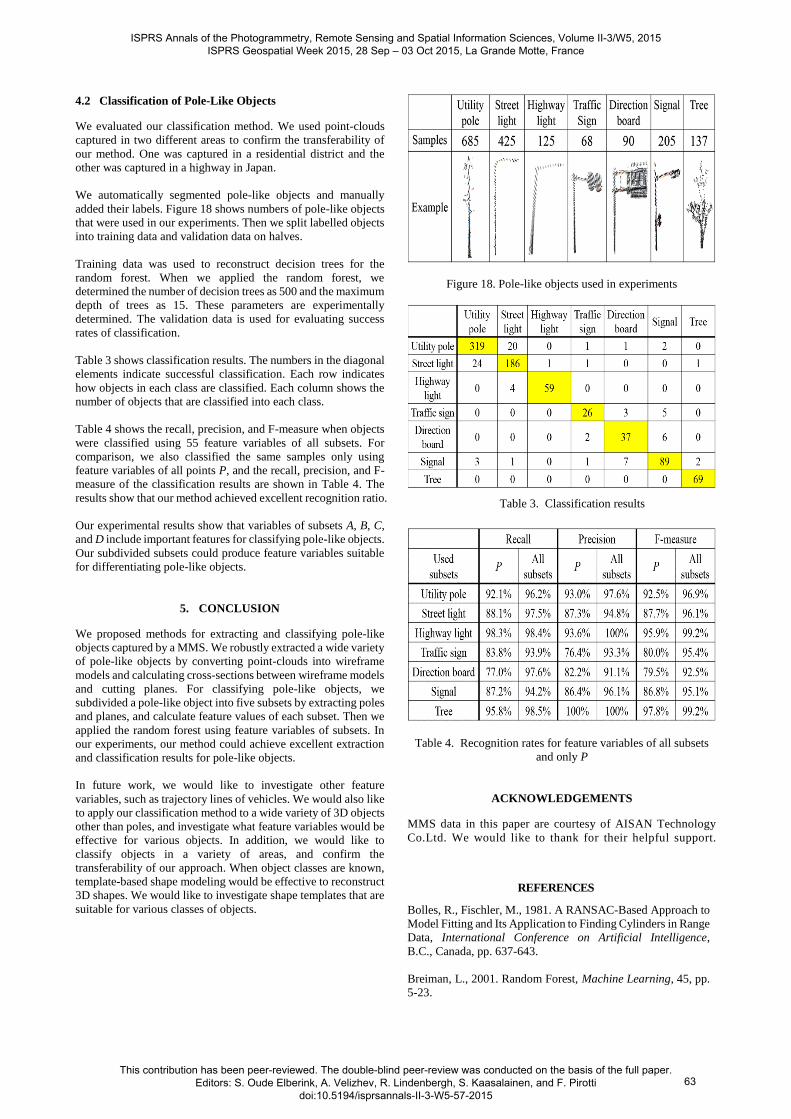
We automatically segmented pole-like objects and manually

added their labels. Figure 18 shows numbers of pole-like objects

that were used in our experiments. Then we split labelled objects

into training data and validation data on halves.

Training data was used to reconstruct decision trees for the

random forest. When we applied the random forest, we

determined the number of decision trees as 500 and the maximum

depth of trees as 15. These parameters are experimentally

determined. The validation data is used for evaluating success

rates of classification.

Table 3 shows classification results. The numbers in the diagonal

elements indicate successful classification. Each row indicates

how objects in each class are classified. Each column shows the

number of objects that are classified into each class.

Table 4 shows the recall, precision, and F-measure when objects

were classified using 55 feature variables of all subsets. For

comparison, we also classified the same samples only using

feature variables of all points P, and the recall, precision, and F-

measure of the classification results are shown in Table 4. The

results show that our method achieved excellent recognition ratio.

Our experimental results show that variables of subsets A, B, C,

and D include important features for classifying pole-like objects.

Our subdivided subsets could produce feature variables suitable

for differentiating pole-like objects.

5. CONCLUSION

We proposed methods for extracting and classifying pole-like

objects captured by a MMS. We robustly extracted a wide variety

of pole-like objects by converting point-clouds into wireframe

models and calculating cross-sections between wireframe models

and cutting planes. For classifying pole-like objects, we

subdivided a pole-like object into five subsets by extracting poles

and planes, and calculate feature values of each subset. Then we

applied the random forest using feature variables of subsets. In

our experiments, our method could achieve excellent extraction

and classification results for pole-like objects.

In future work, we would like to investigate other feature

variables, such as trajectory lines of vehicles. We would also like

to apply our classification method to a wide variety of 3D objects

other than poles, and investigate what feature variables would be

effective for various objects. In addition, we would like to

classify objects in a variety of areas, and confirm the

transferability of our approach. When object classes are known,

template-based shape modeling would be effective to reconstruct

3D shapes. We would like to investigate shape templates that are

suitable for various classes of objects.

Figure 18. Pole-like objects used in experiments

Table 3. Classification results

Table 4. Recognition rates for feature variables of all subsets

and only P

ACKNOWLEDGEMENTS

MMS data in this paper are courtesy of AISAN Technology

Co.Ltd. We would like to thank for their helpful support.

REFERENCES

Bolles, R., Fischler, M., 1981. A RANSAC-Based Approach to

Model Fitting and Its Application to Finding Cylinders in Range

Data, International Conference on Artificial Intelligence, B.C., Canada, pp. 637-643.

Breiman, L., 2001. Random Forest, Machine Learning, 45, pp.

5-23.




63

Cabo, C., Ordonez, C., Garcia-Cortes, S., Martinez, J., 2014. An

algorithm for automatic detection of pole-like street furniture

objects from Mobile Laser Scanner point clouds, ISPRS Journal

of Photogrammetry and Remote Sensing, Vol. 87, pp. 47–56.

Chen, Y.-Z., Zhao, H.-J., Shibasaki, R., 2007. A Mobile System

Combining Lasers Scanners and Cameras for Urban Spatial

Objects Extraction, In: International Conference on Machine

Learning and Cybernetics, Hong Kong, China, Vol. 3, pp.

1729-1733.

Fukano, K., Masuda, H., 2014. Geometric Properties Suitable for

Classification of Pole-like Objects Measured by Mobile Mapping

System, Journal of Japan Society of Civil Engineers, 70, pp.40-

47.

Golovinskiy, A., Kim, V., Funkhouser, T., 2009. Shape-Based

Recognition of 3D Point Clouds in Urban Environments,

International Conference on Computer Vision, Kyoto, Japan,

pp. 2154-2161.

Ishikawa, K., Tonomura, F., Amano, Y., Hashizume, T., 2012.

Recognition of Road Objects from 3D Mobile Mapping Data,

Asian Conference on Design and Digital Engineering, Niseko,

Japan, No. 100101.

Kamal, A., Paul, A., Laurent, C., 2013. Segmentation based

classification of 3D urban point clouds: A super-voxel based

approach with evaluation, Remote Sensing, 5(4), pp.1624-1650.

Kim, Y.-M., Mitra, N.-J., Yan, D., Guibas, L., 2012. Acquiring

3D Indoor Environments with Variability and Repetition,

Transactions on Graphics, 31(6), pp. 138:1-138:11.

Lai, K., Fox, D., 2009. 3D laser scan classification using web data

and domain adaptation, Robotics: Science and Systems V, Seattle,

USA, pp. 1-8.

Li, D., Oude, Elberink, S., 2013. Optimizing detection of road

furniture (pole-like objects) in mobile laser scanner data, ISPRS

Annals of the Photogrammetry, Remote Sensing and Spatial

Information Sciences. Vol. II, Part 5/W2, pp. 163-168.

Lin, H., Gao, J., Zhou, Y., Lu, G., Ye, M., Zhang, C., Liu, L.,

Yang, R., 2013. Semantic Decomposition and Reconstruction

of Residential Scenes from Lidar Data. ACM Transactions on

Graphics, 32(4), pp. 66:1-66:10.

Masuda, H., Oguri, S., He, J., 2013. Shape Reconstruction of

Poles and Plates from Vehicle based Laser Scanning Data,

Informational Symposium on Mobile Mapping Technology,

Tainan, Taiwan.

Masuda, H., He, J., 2015. TIN Generation and Point-cloud

Compression for Vehicle-Based Mobile Systems. Advanced

Engineering Informatics, to appear.

Mitsubishi Electric, 2012. Mobile Mapping System – High-

accuracy GPS Mobile Measurement Equipment,

http://www.mitsubishielectric.com/bu/mms/.

Munoz, D., Bagnell, J. A., Vandapel, N., Hebert, M., 2009.

Contextual classification with functional max-margin markov

networks. Computer Vision and Pattern Recognition, 2009.

CVPR 2009. IEEE Conference, Miami, FL, USA, pp. 975-982.

Nan, L., Sharf, A., Zhang, H., Cohen-Or, D., Chen, B., 2010.

SmartBoxes for Interactive Urban Reconstruction,

Transactions on Graphics, 29(4), pp. 93:1-93:10.

Nan, L., Xie, K., Sharf, A., 2012. A Search-Classify Approach

for Cluttered Indoor Scene Understanding, Transactions on

Graphics, 31(6), pp. 137:1-137:10.

Oude, Elberink, S., Kemboi, B., 2014. User-assisted object

detection by segment based similarity measures in mobile laser

scanner data. ISPRS International Archives of the

Photogrammetry, Remote Sensing & Spatial Information

Sciences, Zurich, Switzerland, Vol. XL, Part 3, pp. 239-246

Pu, S., Rutzinger, M., Vosselman, G., Elberink, S. O., 2011.

Recognizing basic structures from mobile laser scanning data for

road inventory studies, ISPRS Journal of Photogrammetry and

Remote Sensing, Vol. 66(6), pp. S28-S39.

Puttonen, E., Jaakkola, A., Litkey, P., Hyyppä, J., 2011. Tree

classification with fused mobile laser scanning and hyperspectral

data. Sensors, 11(5), pp.5158-5182.

Taubin, G., 1995. A Signal Processing Approach to Fair Surface

Design, ACM SIGGRAPH, pp. 351-358.

Weinmann, M., Jutzi, B., Mallet, C., 2014. Semantic 3D scene

interpretation: a framework combining optimal neighborhood

size selection with relevant features. ISPRS Annals of the

Photogrammetry, Remote Sensing and Spatial Information

Sciences, Zurich, Switzerland, Vol. II, Part 3, pp. 181-188.

Yang, B., Dong, Z., Zhao, G., Dai, W., 2015. Hierarchical

extraction of urban objects from mobile laser scanning data,

ISPRS Journal of Photogrammetry and Remote Sensing, Vol. 99,

pp. 45–57.

Yokoyama, H., Date, H., Kanai, S., Takeda, H., 2011. Pole-like

Objects Recognition from Mobile Laser Scanning Data Using

Smoothing and Principal Component Analysis, ISPRS-

International Archives of the Photogrammetry, Remote Sensing

and Spatial Information Sciences, Vol. XXXVIII, Part 5-W12,

Calgary, Canada, pp. 115-120.

Zhu, X., Zhao, H., Liu, Y., Zhao, Y., Zha, H., 2010. Segmentation

and classification of range image from an intelligent vehicle in

urban environment, The 2010 IEEE/RSJ International

Conference, Taipei, Taiwan, pp.1457-1462.




64

Documents

DETECTION AND CLASSIFICATION OF POLE-LIKE OBJECTS …