No. 9109

DETECTING LEVEL SHIFTS IN TIME SERIES:MISSPECIFICATION AND A

PROPOSED SOLUTION

by

Nathan S. Balke*

Research Paper

Federal Reserve Bank. of Dallas

This publication was digitized and made available by the Federal Reserve Bank of Dallas' Historical Library (FedHistory@dal.frb.org)

No. 9109

DETECTING LEVEL SHIFTS IN TIME SERIES:MISSPECIFICATION AND A

PROPOSED SOLUTION

by

Nathan S. Ba1ke*

June 1991

*Assistant Professor of Economics, Southern Methodist University, Dallas,Texas and Visiting Scholar, Research Department, Federal Reserve Bank ofDallas. I would like to thank Tom Fomby for many helpful discussions and muchencouragement and Mark Wynne for comments on a previous draft. Ellah Pinahelped with the manuscript and tables. The views expressed in this paper aresolely those of the author and should not be attributed to Southern MethodistUniversity or to the Federal Reserve Bank of Dallas or the Federal ReserveSystem.

,

Detecting Level Shifts in Time Series:

Misspecification and a Proposed Solution'

Nathan S. Balke

Assistant Professor of EconomicsSouthern Methodist University

and

Research AssociateFederal Reserve Bank of Dallas

June 1991revised September 1991

Abstract This paper demonstrates the difficulty that traditionalspecification, estimation, detection, and removal outlier detection methodshave in identifying level shifts in time series. A simple modification tothe well-known outlier/level shift detection algorithm described in Tsay(1988) is proposed that dramatically improves the ability to correctlyidentify level shifts. This modification involves combining an outliersearch that is initialized by an ARMA(O,O) model with an outlier search thatemploys a traditionally specified ARMA model. The results of the outliersearches are used to specify a single intervention whose final specificationis then determined by stepwise reduction. This "combinejreduce ll approach isrelatively easy to implement and appears to be quite effective in practice.

Key Words: Level shifts, outliers, ARMA models, intervention models

I would to like thank Tom Fomby for many helpful discussions and muchencouragement and Mark Wynne for comments on a previous draft. Shengyi Guoprovided excellent research assistance. Ellah Pina helped with themanuscript and tables. The views expressed in this paper are solely those ofthe author and should not be attributed to the Federal Reserve Bank of Dallasor the Federal Reserve System.

1

1. Introduction

Anomalies such as outliers and level shifts are quite common in time

series data. For example, Balke and Fomby (1991) examined fifteen

macroeconomic time series and found outliers and/or level shifts in almost

every series. These extraordinary observations (or sequence of extraordinary

observations) are often associated with identifiable events such as wars,

strikes, and changes in policy regimes. In addition, the presence of

outliers and level shifts pose problems for the identification and estimation

of ARIMA models, see Chang (1982), Chang, Tiao, and Chen (1988), and Chen and

Tiao (1990). If the type and dates of these disturbances were known, their

effects could be controlled with intervention analysis, as in Box and Tiao

(1975). In practice, however, the type and date of an intervention is seldom

known a priori.

As a result, methods of identifying and correcting for outliers and

level shifts in time series have recently attracted much interest. Among the

several approaches include robust estimation techniques (Martin (1980)),

Bayesian analysis (Abraham and Box (1979), McCulloch and Tsay (1991)), and

"leave-k-out" diagnostics (Bruce and Martin (1989)). In addition, iterative

procedures proposed and employed by Chang (1982), Tsay (1986), and Chang,

Tiao, and Chen (1988) have been used with success in the identification of

outliers when the number and times of the disturbances are unknown. These

iterative procedures have also been adapted for identification of level

shifts (Chen and Tiao (1990)). Tsay (1988) provides a unified treatment of

outliers and level shifts in the context of these iterative procedures. The

procedure outlined by Tsay is particularly useful for applied work· because it

is quite flexible (it can be used to search for both additive and innovative

2

outliers as well as level shifts) and is relatively easy to implement.

Unfortunately, as I show below, the procedure suggested by Tsay (1988)

does not always perform satisfactorily when level shifts are present. The

iterative procedure described by Tsay consists of several distinct steps:

specifying and estimating an initial ARMA model, detecting outliers based on

a prespecified criteria, removing the outliers, and then respecifying and

reestimating the ARMA model. This sequence is repeated until no remaining

outliers are detected. However, the presence of level shifts causes serious

problems in the specification and estimation of the initial ARMA model (Chen

and Tiao (1990» which in turn affects the subsequent detection and removal

steps. As a consequence, the procedure described by Tsay may misidentify

outliers and level shifts.

To deal with this misspecification problem, I suggest a simple

modification to the outlier identification approach of Tsay. The

modification is as follows:

(i) In addition to conducting an outlier search based on specifying and

estimating an initial ARMA model as originally proposed in Tsay (1988),

a separate search employing an ARMA(O, 0) - -or "white noise" - -model as the

initial ARMA specification is conducted.

(ii) The results from the two outlier searches are combined to form a

single intervention model (Box and Tiao (1975». The final

specification is determined by a stepwise reduction of this

comprehensive intervention model.

This "comb ine/reduce" (hereafter CR) approach appears to be much more capable

of handling level shift outliers than is the original Tsay procedure.

The remainder of the paper is organized as follows. In Section 2, I

3

present two examples using actual data that demonstrate the difficulty the

Tsay procedure can have in correctly identifying level shifts and the

improvement offered by the CR method proposed here. Section 3 describes the

outlier search procedure examined in Tsay (1988) in more detail. The

analytical and Monte Carlo analyses in Section 4 document the problems that

level shifts pose for the traditional outlier search method. In particular,

I examine the sensitivity of the outlier search with respect to the choice of

the initial ARMA specification. In Section 5, I outline a simple

modification to the Tsay (1988) outlier search that was employed on the two

data series examined in Section 2. Two seperate Monte Carlo experiments

suggests that this modification results in a substantial improvement in the

Tsay procedure when level shifts are present.

2. Some Examples

To motivate the problem that level shifts pose for the outlier

identification procedure described by Tsay (1988) and the potential

effectiveness of the proposed modification, I consider two examples.

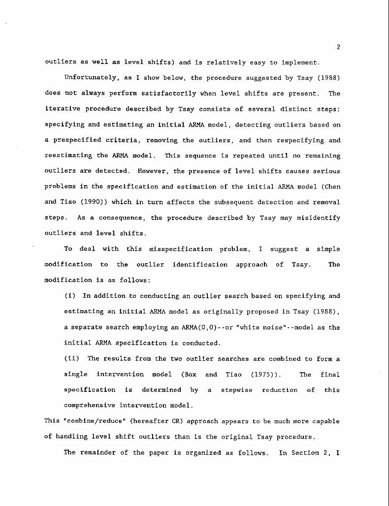
First, consider the quarterly compensation per hour for the nonfarm

business sector in logarithms (series LBCPU from CITIBASE). The Tsay outlier

search procedure results in the following specification for the sample 19S8Q1

to 1990Q2:

(1) (1 - B)Yt - .008 A01960Qlt( .003)

+ [1/(1 - .243B - .234B2 - .229B'(.090) (.091) (.090)

,a. - .0046,

.1SlB')] [ .002 + at](.089) (.001)

where BiXt - Xt - i , and the standard errors are in parentheses. A01960Qlt is

4

an additive outlier intervention with A01960Ql - 1 when t - 1960Ql and 0

otherwise. Figure 1a plots compensation per hour, nonfarm business and the

outlier component for the Tsay procedure (the unconditional sample mean of

the series has been added to the outlier component).

On the other hand, following the combine/reduce (CR) outlier procedure

described briefly in the introduction and in more detail in Section 5 leads

to the following specification:

(2) (1 - B)Yt .007 LS1968Qlt(.001)

+ .005 LS1972Q4t( .001)

.012 LS1982Q2t(.001)

A

". - .0041,

+ .013 A01960Qlt +(.004)

[1/(1 - .127B) J [.009 + at],(.089) (.001)

where LS1968Qlt, LS1972Q4t , and LS1982Q2t are level shift interventions in

which LSdatet - 1 , t ~ date, 0 otherwise. Figure Ib plots compensation and

the outlier/level shift component (with unconditional mean added) for the CR

procedure. These level shifts correspond to the height of the Vietnam War

buildup, the 1972-73 expansion, and the "Volcker disinflation" of 1982. Not

only are these level shifts present in the compensation data, but they also

appear to be present (at very similar dates) in other inflation series such

as the Consumer Price Index and the GNP deflator (Balke and Fomby (1991».

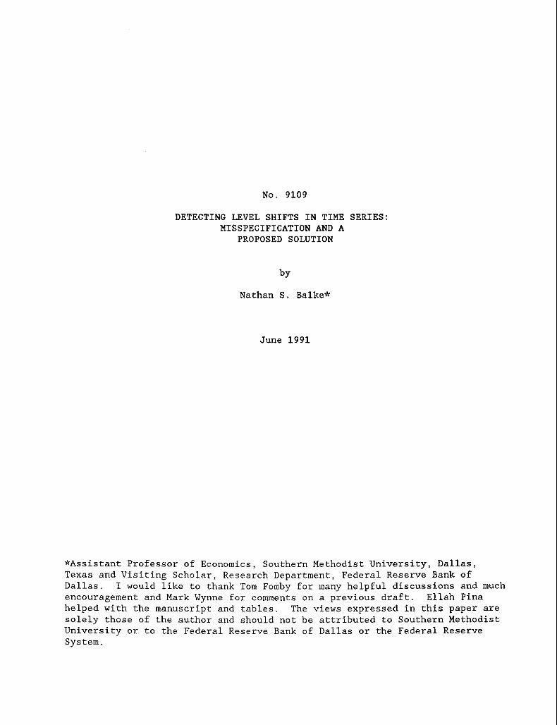
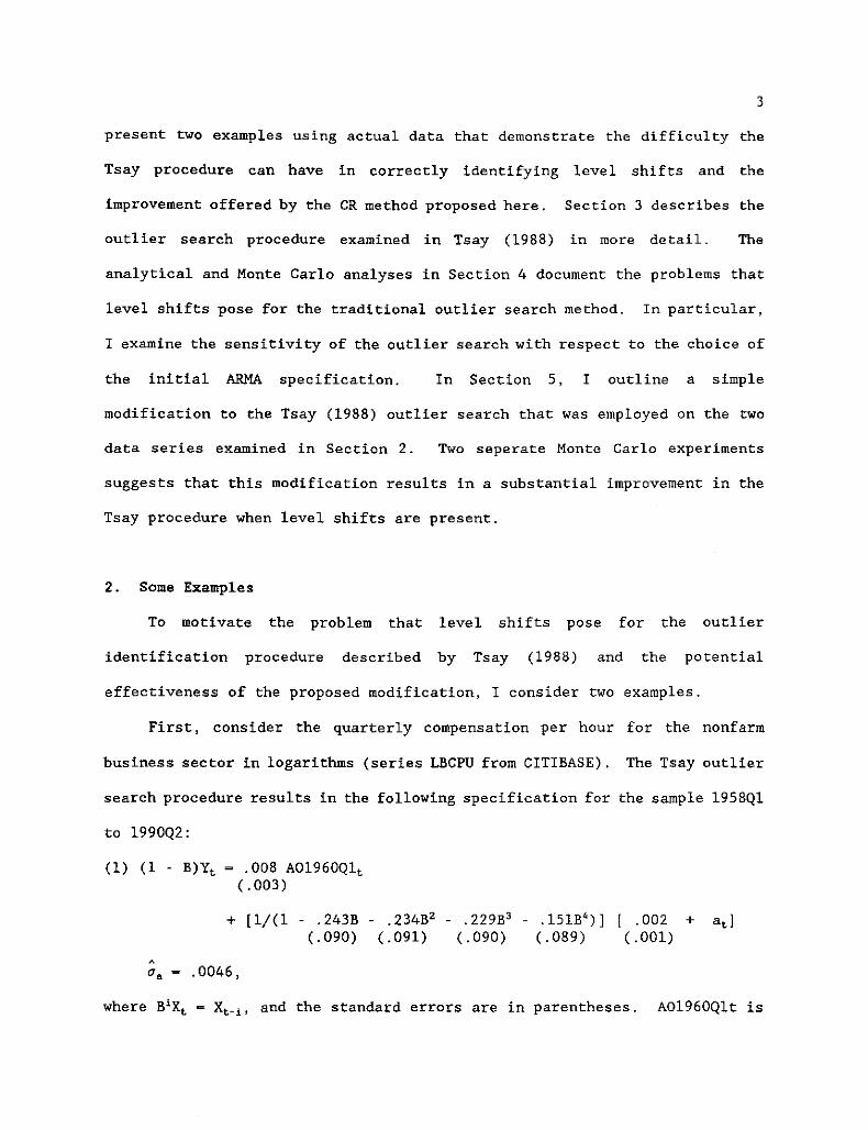
Second, consider the monthly series for car drivers killed and seriously

injured in the United Kingdom (U.K.), in logarithms and with monthly means

extracted, from January 1969 to December 1984. Harvey and Durbin (1986)

examined the killed and seriously injured series to assess the effects of a

U.K. seat belt law that went into effect in February 1983. These data are

published in Harvey (1989), Appendix 2. Using an intervention model (the

intervention variable also includes an anticipatory effect for January 1983),

5

Harvey and Durbin found that the introduction of a seat belt law in 1983

caused a significant reduction in traffic accident casualties.

The Tsay outlier search implies the following final intervention model

[1/(1 - .426B - .308B2(.071) (.074)

.145B3 ) ]

( . 070)-.285 I01983Feb t + at ],(.073 )

0". - .073,

where I01983Febt - 1 if t - February 1983, 0 otherwise. Figure 2a plots the

killed and seriously injured series as well as the outlier component implied

by the Tsay procedure.

intervention model

In contrast, the CR procedure yields the final

(4) Yt - .132 LS1970Febt( .014)

.155 LS1974Novt( .017)

.199 LS1983Jant(.023)

+ [1/(1 - .208B - .167B2)] at,(.073) (.073)

,0". .067.

Figure 2b plots the killed and seriously injured series and outlier component

for the CR procedure.

While both models suggest a sharp reduction in injuries during 1983, the

Tsay outlier search identifies this reduction as an innovative outlier and as

such represents a temporary reduction, while the CR procedure implies a level

shift intervention and a permanent reduction. The combined outlier search

suggests two additional important level shifts (LS1970Feb and LS1974Nov) not

identified by the Tsay outlier search. The November 1974 level shift

probably reflects the effects of the jump in energy prices that occurred

during 1974. McCulloch and Tsay (1991) found level shifts very similar to

those found here (February 1970, January 1975, January and February 1983)

using Bayesian analysis employing a Gibbs Sampler.

Thus, for both data sets, the outlier search procedure described by Tsay

6

(1988) fails to correctly identify some very plausible level shifts. In the

first series t the Tsay outlier search misses what appear to be level shifts,

while in the second series the Tsay outlier search identifies a probable

level shift as an innovative outlier.

3. The Tsay iterative outlier search procedure

Consider the following outlier model described in Tsay (1988). Let

(5) Yt f(t) + Zt,

where Zt (O(B)/4>(B))at , and at is a Gaussian variate with zero mean and

variance a'.. O(B) ~ 1 - 0lB - 0,B2 - ••• - 0lBQ, and 4>(B) - 1 - 4>lB - 4>2B2 -

- 4>lBP. One can think of Zt as the regular component of the time series

The variable f(t) contains anomalous exogenous disturbances such as

outliers and level shifts. Again following Tsay (1988), let

(6) f(t) - Wo (w(B)/o(B)) €~d,>

where €~d~ 1 if t - d and 0 otherwise indicates whether a disturbance occurs

at time d. weB) and o(b) are backshift polynomials that describe the dynamic

effect the disturbance has on Yt . When (w(B)/o(B)) - 1, the disturbance is

an additive outlier (AO); when (w(B)/o(B)) - (O(B)/4>(B)), the disturbance is

an innovative outlier (10); when (w(B)/o(B)) - l/(l-B), the disturbance is a

level shift (LS).

To help identify the presence of outliers and level shifts, Tsay (1988)

proposes several statistics. Define Yt - (4)(B)/O(B))Yt . Define ~(B) - 1 ­

~lB - "'2B2 - ... - 4>(B)/O(B), and '1(B) - 1 - '11B - '12B2 - .,. - ",(B)/(l-B).

Tsay suggests the following test statistics for the various types of

outliers:

7

Am,t Yt/U..

AAO,t P2A,t(Yt - <_,<;T-t "<YtH)/(PA,tU.), and

ALS,. P2L,.(Yt <_,<;T-t '1<YtH)/(PL,tu.),

where p 2A,t - (1 + <_,<;T-t ,,<2)-', p2L,t _ (1 + <_,<;T-t '1<2)-', u2 • is the variance

of at., and T is the sample size. Let Amax =0 max {Aro,max' AAO,max' ALS,max} I where

Aj,m.x - max"tsT (IAj,tl), j - 10, AO, LS. If the Amax statistic exceeds a

prespecified critical value, then an outlier has occurred.

Tsay suggests a sequential algorithm for identifying outliers. First,

estimate an ARMA model and extract the residuals and the residual variance.

Second, search for outliers in the residuals using the statistics described

above. If an outlier is found, remove the effect of the outlier and

recalculate the residuals and residual variance. Continue searching and

adjusting until no more outliers are indicated. Reestimate the ARMA model

using the adjusted series and extract the residuals. Once again, search for

outliers. Stop the algorithm when no additional outliers are found.

4. ARMA specification and outlier identification

Note that the initially estimated ARMA model is the correct

specification of the regular dynamics «8(B)/¢(B)at) under the null

hypothesis of no outliers. If, however, outliers are found, then the initial

ARMA model for the regular component will be misspecified. Unfortunately,

misspecification of the initial ARMA model can lead to misidentification of

outliers. In particular, series in which a level shift is present will

exhibi t a high degree of serial corre lation regardless of the regular

dynamics (Chen and Tiao (1990)). In this case, the initial ARMA model for

the regular dynamics implies greater serial correlation than is in fact the

8

case; therefore, the residuals from this model will not reflect the true

nature of the outlier.

To see the dangers of this misspecification, consider the following

example. Let ~(B) - 1 ~B and 8(B) - 1.

Yt [l/(l-~B)l at, t:5T"

Yt [l/(l-~B) J at + j.l, t > T, .

The size of level shift is given by j.l, and it occurs at T, + 1. The sample

size is given by T. Subtracting the sample mean of the series yields

Yt y [l/(l-~B)] (at a) j.l(T-T, )/T, t :5 T"

Yt y [l/(l-~B)] (at a) + j.lT, /T, t > T"

where a - (l-~) t=lL:T[l/(l-~B) ] adT.

Suppose we estimate an AR(l) model for Yt . Let Yt Yt - Y. The least

squares estimate of the autoregressive parameter,

is inconsistent when j.l # O. Keeping the proportion of the sample before (and

after) the level shift date constant (that is (T-T,)/T and T, /T are constant)

as the sample size increases,

A

(8) pUm ~

where

Notice that the presence of level shifts causes the autoregressive parameter

to be overestimated asymptotically. The degree of the overstatement depends

on the variance of the regular component (u2a/(1-~2» relative to the variance

of the level shift component (j.l2(T-T, )T,/T2). The larger the variance of the

level shift component (that is, the larger the level shift), the more the

autoregressive estimate is biased. Table 1 provides an indication of how

9

serious this bias can be.

This misspecification of the ARMA model in the presence of level shifts

affects the outlier statistics in several ways. First, as mentioned above,

the residuals from the ARMA model will not truly reflect the outlier or level

shift. Second, the filter used to generate the oX statistics will be

misspecified.

In Table 2, a limited Monte Carlo experiment indicates the effects of

this misspecification (see Appendix A for a detailed description of this

experiment). Here, a level shift occurs halfway through the sample, and the

outlier search follows the procedure described in the previous section in

which an ARMA model is estimated first; the initial specification of the ARMA

was set as an AR(l). Table 2 indicates the number of samples in which the

algorithm identified outliers of the various types and whether the identified

outliers were on, close to (T1+l ± 5), or not close to the actual date in

which the level shift occurred. For all experiments, the variance of the

regular component is fixed at 1, while the size of the level shifts and the

AR(l) coefficient varies. The critical value for the outlier classification

was set at 3. Note that it is possible for the outlier procedure to identify

several different outliers for a given sample (replication), which explains

why adding up the identified outliers may exceed the number of Monte Carlo

replications for some parameter settings.

The Monte Carlo experiments described in Table 2 suggest that the

traditional approach of estimating an ARMA model first does not always yield

satisfactory results when a level shift is present. For small level shifts

(~- 1 and ~ - 2), the outlier algorithm might miss the level shift entirely.

For larger level shifts (~- 3 and ~ - 5), the outlier algorithm will often

misidentify the level shift as an innovative outlier.

10

This is especially

true as the persistence of the regular component increases (compare as <p

moves from 0 to 0.8). For example, when p - 5 and ~ - 0.8, estimating the

ARMAmodel first causes the outlier algorithm to correctly identify the level

shift in only 6 percent of the samples while it identifies an innovative

outlier instead of a level shift in 94 percent of the samples. In addition,

even after the outliers have been identified and removed, the autoregressive

parameter of the AR model is still overestimated. This is particularly true

when the level shift is large. Additional Monte Carlo work not reported here

and the analysis below suggests that the misspecification is even more likely

if the level shift occurs early in the sample.

However, suppose that instead of estimating an ARMA model first, no ARMA

filter is applied to the data except for extracting the mean of the series

(or a time trend if one is present). That is, the initial ARMA model is

specified as white noise. Table 3 contains the results of the same Monte

Carlo experiment as in Table 2 except the initial ARMA model was specified as

white noise. After the first iteration of the outlier search, an ARMA model

(here, an AR(l)) was estimated for subsequent iterations as in the

traditional approach.

The results in Table 3 imply that when starting with the white noise

ARMA model, the outlier algorithm correctly identifies the level shift more

times than starting with an estimated ARMA model. Not only is the white

noise model more likely to capture small level shifts, but it is also much

less likely to misidentify a level shift as another type of outlier. The

abili ty to identify level shifts when starting from the white noise ARMA

model is not particularly sensitive to the specification of the regular

11

component (as long as the unconditional variance of the regular component is

held constant). Furthermore, comparing Tables 2 and 3 reveals that the final

estimated AR coefficient is often closer to the true parameter when the white

noise model is used than when an ARMA model is used in the initial iteration;

this is especially true for large level shifts. Thus, starting with the

white noise ARMA model may improve the ability of the outlier identification

algorithm to correctly identify level shifts and to estimate the systematic

dynamics.

Unfortunately, there are some drawbacks to initializing the algorithm

with the white noise model. First, as Table 3 demonstrates, starting with

the white noise model tends to identify too many level shifts. The spurious

identification of level shifts is more severe as the persistence in the

regular component increases (see p 5 and ~ - 0.8, for example). Second,

the white noise model by construction is incapable of distinguishing between

innovative and additive outliers. In fact, as I show below, innovative

outliers tend to show up as a sequence of additive outliers.

To further understand the differences between starting the outlier

algorithm with an estimated ARMA model and starting with a white noise model,

consider the properties of the outlier statistics both under the null

hypothesis of no outliers or level shifts and under the alternative

hypothesis of a level shift. Denote the innovative and level shift outlier

statistics when an AR(l) is estimated by AARra T1+1 and AARLS •T1+1 while the

statistics for the white noise are denoted by Ah'NAO ,I1+1 and )"WNLS ,T1+1"

Consider the example described above. Under the null hypothesis of no

outliers or level shifts (p. - 0), AAR,O T1+1' AARLS Tl+1 and A"'\O Tl+1 - AN (0,1) ,

where AN denotes asymptotic normality. On the other hand, while E[A"'\S Tl+1]

12

- 0, in large samples

Var[>.WI\S,Tl+tl "" 1 + 2 i_1:ET-Tl-1 (T-T1-i)/(T-T1) q,i.

Serial correlation in the systematic dynamics prevents the asymptotic

distribution of AWNLS T1+l from being standard normal, because the denominator

of >.WNLS T1+1 is too low when q, > O. In other words, the standard error of the

white noise, level shift estimate understates the true standard error when q,

> O. This explains why in the Monte Carlo experiment the white noise model

found too many level shifts for cases in which q, was relatively large.

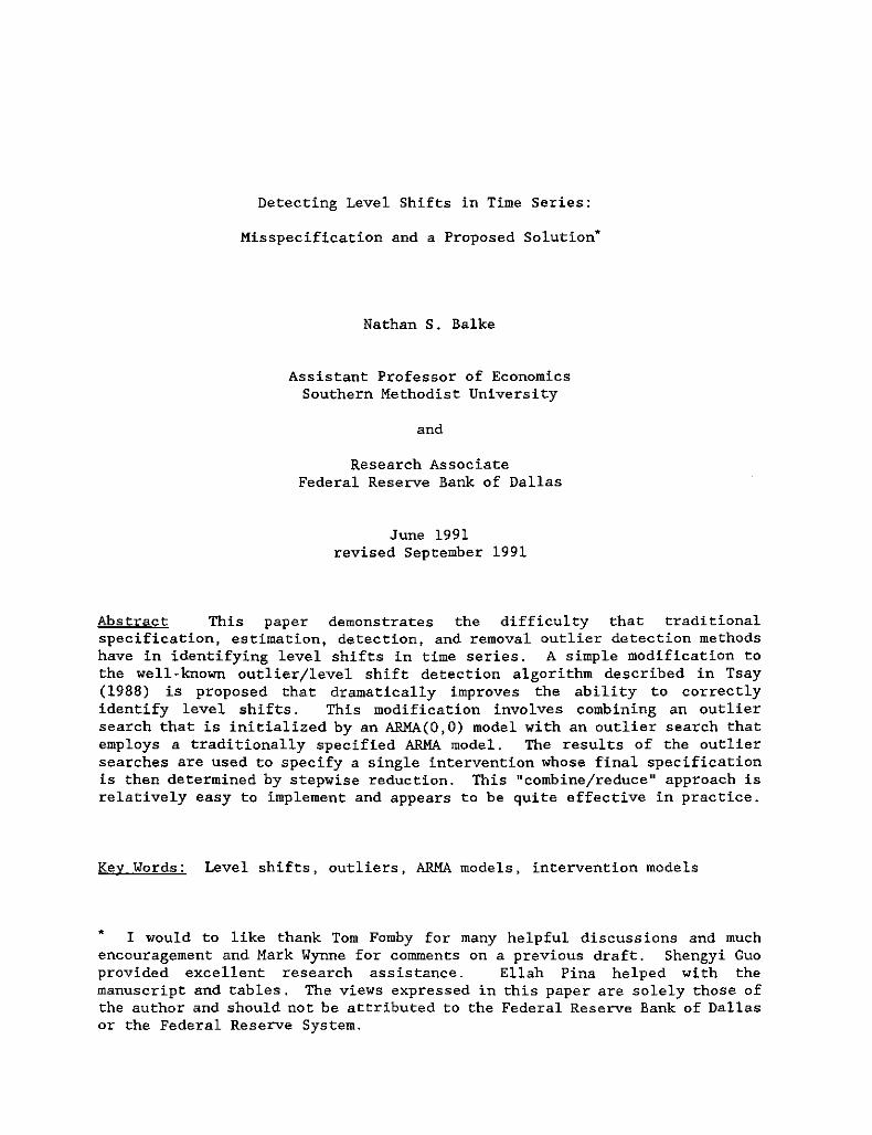
When a level shift occurs (that is, ~ ~ 0), the expected value of the

various statistics at the shift date, T1+l, (taking the estimated parameters

of the ARMA model as given) are

A A

E[>.ARro ,T1+1l [~TtlT + q,1'(T-T1)/T l/a.,

.... 2 A .... .... "-

E[>.ARLs ,T1+1] P L,T1+d~TtlT + q,1'(T-T1)/T + (1-q,)Z(T-T1-l)I'TtiTj/(Pt,T1+1 a.),

A

E[>.WNAo,T1+tl (~Tl/T)/a, and

E[>.WNLS T1+tl (I'T1/T)/(;z/(T-T1»"/Z,

where ~ZL Tl+l = (1 + (l-~)Z(T-Tl-l»,

pUm ;z. _ aZ• + (q,_~)zaz./(l_q,Z) + (l-~)Z~Z(T-Tl)Tl/TZ, and

pUm ;z _ aZ.!(l_q,z) + I'z(T-T1)TtlTz.

Note that misspecification of the initial ARMA model has a direct effect on

the expected value of the outlier statistics of the AR(l) model,

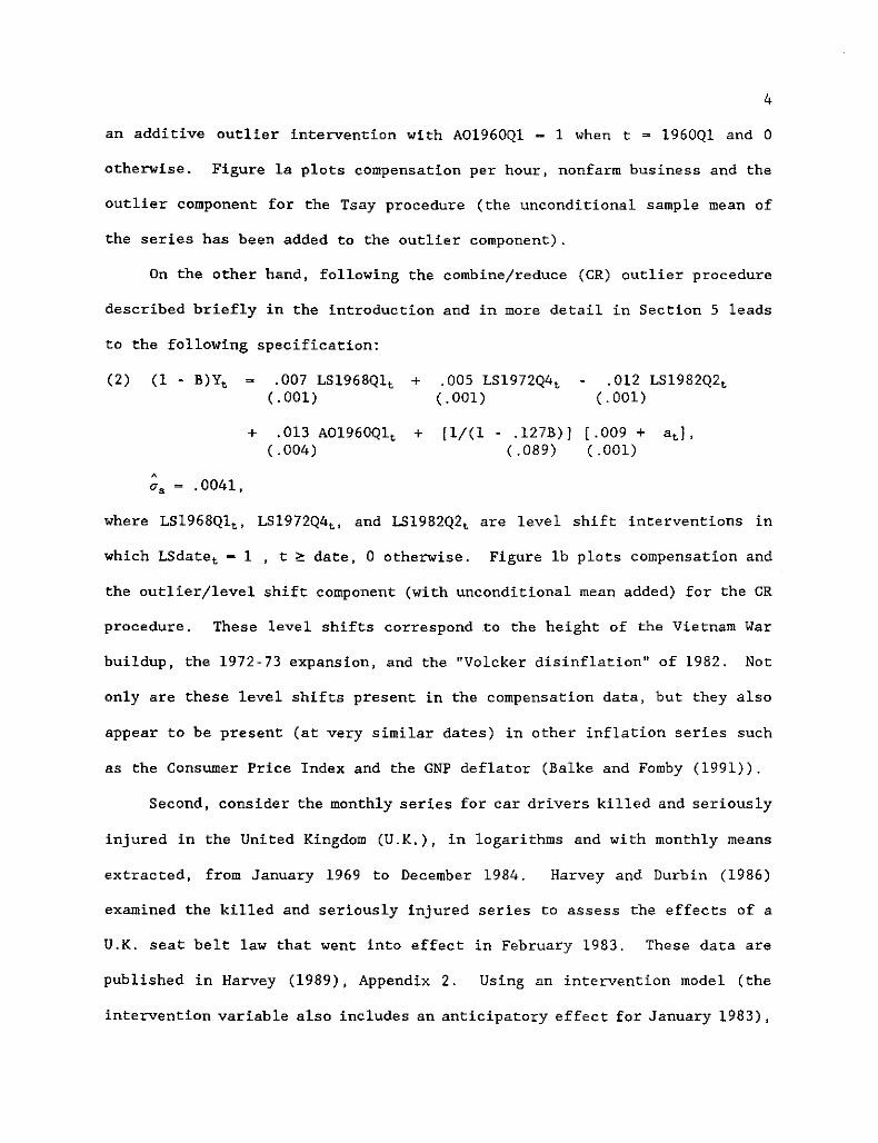
The >. statistics for various level shift sizes are plotted in Figure 3.

Figure 3 shows that the white noise level shift statistic is more sensitive

to small level shifts than the ARMA model statistics are. In fact, for a

critical value of 3, the expected level shift statistics imply that the white

noise model can detect a smaller ~ than can the search in which an ARMA model

is estimated first. Furthermore, when the level shift occurs early in the

13

sample (consider the cases in which T, - 25 with T ~ 100), EpARro ,T1+1] is

often greater than E[>.ARLS ,T1+1]' This suggests that starting with an ARMA

model will systematically misidentify level shifts as innovative outliers.

As ¢ gets larger, this tendency of the ARMA outlier search to misidentify

level shifts as innovative outliers increases. For the case in which T1 = 50

(and higher), E[>.ARro ,T1+,] approaches E[,\ARLS ,T1+,] as the size of the level

shift increases and as ¢ increases, at least with respect to the expected

values of the test statistics. Thus, the search beginning with an estimated

ARMA model is not as sensitive to small level shifts as the white noise

search is, and it is more likely to misclassify a level shift as an

innovative outlier if the level shift occurs early in the sample and if ¢ is

relatively high. These results are consistent with the Monte Carlo

experiment presented in Tables 2 and 3.

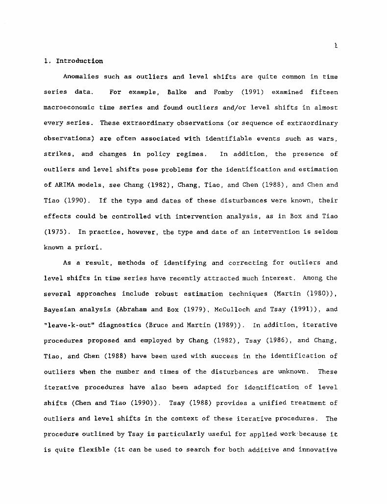
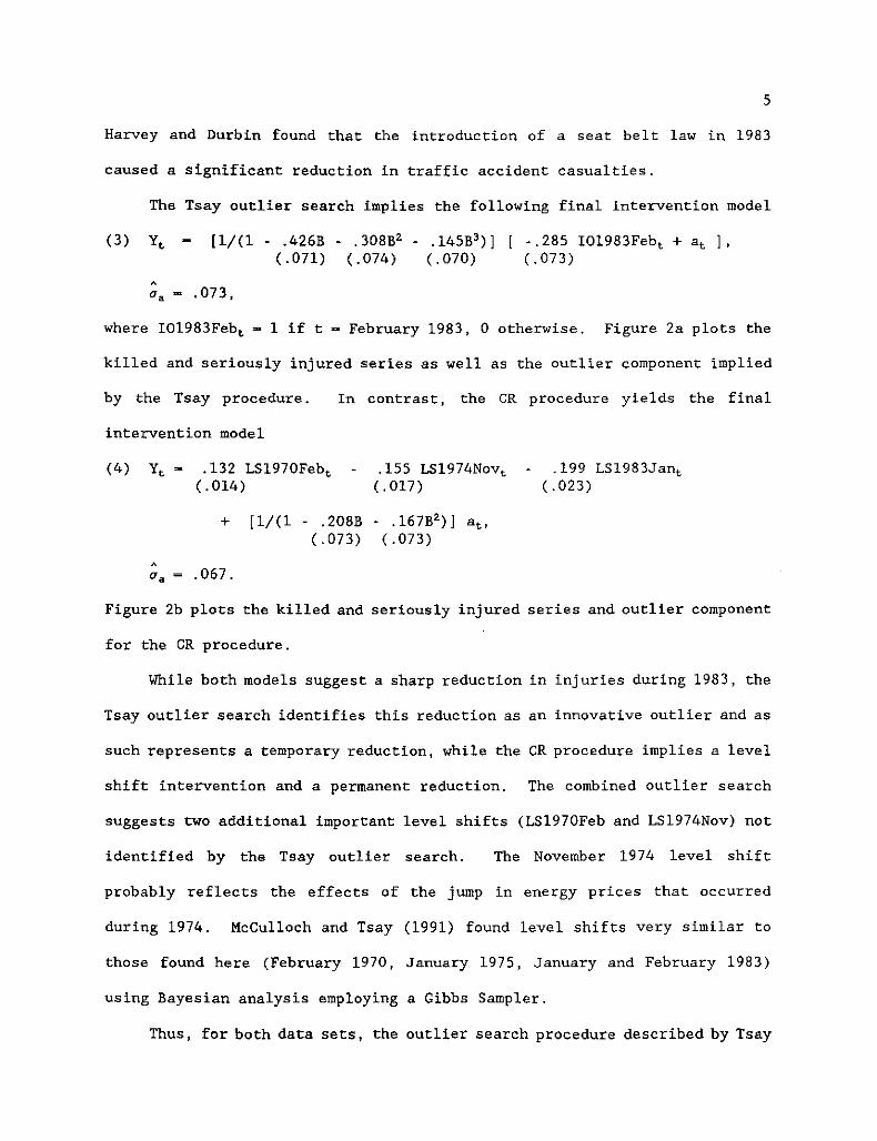
If there is an innovative or additive outlier rather than a level shift,

how do the various statistics perform? Tsay (1986, 1988) and Chang, Tiao,

and Chen (1988) suggest that the traditional approach does fairly well in

identifying and distinguishing innovative and additive outliers. While the

white noise initialization is incapable of modeling an innovative outlier in

the initial iteration, it is possible that an innovative outlier could be

captured by a series of additive outliers. For both start-up models, there

appears to be little danger of misclassifying innovative outliers as level

shifts (as long as the outlier does not occur near the end of the sample).

Figure 4 presents the expected outlier statistics for the case in which there

is an innovative outlier at T,+l - 51 (the size of the innovative outlier is

given by pl. From Figure 4, the white noise model is unlikely to classify

that outlier as a level shift; it is much more likely to classify that

14

outlier as an additive outlier.

5. Proposed methodology

It is clear that the outlier search algorithm advocated by Tsay (1988)

has difficulties in the presence of level shifts. As shown above, starting

the outlier search by specifying and estimating an ARMA model can lead to the

misclassification of outliers in the presence of level shifts. Yet, as

demonstrated by Chang, Tiao, and Chen (1988) and Tsay (1986,1988), the above

algorithm is effective in identifying and classifying additive and innovative

outliers. While starting the search by specifying a white noise model leads

to more effective identification of level shifts than with an ARMA model, it

is incapable of distinguishing between additive and innovative outliers (at

least in the first iteration of the outlier search), and it has a tendency to

identify spurious level shifts.

In this section, I describe in detail a simple extension to the outlier

search procedure outlined by Tsay that attempts to take advantage of the

relative strengths of both outlier searches. I also consider two seperate

Monte Carlo experiments to evaluate the proposed procedure. The first

experiment is a conditional experiment where the number and type of level

shifts and outliers is controlled. The second experiment is an unconditional

experiment where the number as well as timing of the various outliers are

determined randomly. Both experiments suggest that proposed procedure

improves upon the basic Tsay methodology when level shifts are present.

5.1 The Combine/Reduce Procedure

The recommended procedure is as follows:

15

(i) Identify potential outliers and level shifts using the outlier

search method suggested in Tsay (1988) but, in addition to starting from an

estimated ARMA model, run the outlier search starting with the white noise

model as well. These two outlier searches will provide a list of potential

outlier and level shift candidates.

(ii) Combine the outliers from the two searches into a single

intervention model while letting the specification of the ARMA model for the

systematic dynamics of the combined intervention model encompass the ARMA

models suggested by the two outlier searches. Estimate this intervention

model. Eliminate the intervention dummy with the lowest t statistic if this

t statistic is lower than a prespecified critical value. Below I use the

same critical value for the t statistic as I use for the outlier search ( It

statl < 3). Reestimate the intervention model. Continue this stepwise

reduction of the intervention model until all intervention variables have t

statistics greater than the specified critical value. Once outliers have

been identified in this way, reduce the ARMA specification by stepwise

reduction (here I use a more strict criteria of elimination: It-statl < 1).

(iii) As a final check, determine whether the outliers or level shifts

coincide with identifiable historical events that could affect the time

series. For example, in Balke and Fomby (1991), we attempt to match outliers

and level shifts in fifteen macroeconomic time series with identifiable

economic events. In practice, the use of historical introspection can be

quite useful in avoiding overparameterizations that may remain after the

stepwise reduction of the combined interventions.

The proposed procedure allows the maximum flexibility in the

identification of outliers by using the two outlier searches. This procedure

16

lessens the danger of misspecification and misidentification of outliers when

level shifts are present. Yet, the stepwise reduction in the intervention

model increases the chances of weeding out spurious outliers and level

shifts. Of course, the standard errors of the final intervention model are

conditional standard errors (as is the case with the Tsay procedure) and,

therefore, may understate the true uncertainty surrounding the parameter

estimates.

5.2 A Conditional Monte Carlo Experiment

To further evaluate the proposed procedure I I ran two separate Monte

Carlo experiments. In the first experiment, I generated twenty- four data

sets, each one corresponding to a particular combination of outliers, level

shifts, and serial correlation in the regular component (these combinations

are listed under the Actual column of Table 4). The sample length was 100

observations. The regular component was specified as an AR(l) with ~ - 0,

0.4, and 0.8, and I set the unconditional variance of the regular component,

a2a/(1-~2), equal to 1. The date at which an outlier or level shift occurs

was randomly determined subject to the constraint that it cannot happen in

the first ten or last ten observations. The size of the outlier or level

shift was drawn from a N(0,3) distribution; draws whose absolute value are

less than 3 are rejected and another draw is taken in order to ensure that an

outlier of sufficient size is present. The value of the AR parameter, the

particular combination of outliers, as well as the date and size of the

outliers were unknown at the time the data was analyzed; a colleague

generously agreed to randomize the data sets so that I did not know the

contents of the data set before the analysis.

17

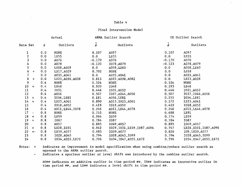
Table 4 summarizes the final specifications obtained by the proposed CR

intervention modeling approach. I compare actual outlier dates with those

indicated by the final intervention model from an ARMA outlier search alone

and with those indicated by the final intervention model from the CR

procedure. The estimated AR(l) coefficients for the regular component are

displayed as well. A 11+" indicates an improvement in the overall

specification from adding the information in the white noise search. A "_"

indicates a case in which using the white noise outlier search adds a

spurious outlier or level shift.

In eight of the twenty-four data sets, including the results of the

white noise outlier search improves the identification and specification of

the final intervention model. In each of these eight cases a level shift was

present. As suggested in the previous section, the ARMA outlier search

sometimes has difficulty when level shifts are present. In data sets 10, 14,

18, 21, and 22, the ARMA search misidentifies level shifts as innovative

outliers. In data sets 6 and 8, the ARMA search misses the level shift

altogether. In addition to providing a better specification of the outliers

and level shifts, including the outliers from the white noise search

dramatically improves the accuracy of the autoregressive parameter estimates

in these data sets. Again, this points out the importance of correctly

capturing the effect of the level shift when estimating the ARMA model. On

the other hand, the white noise outlier search adds spurious outliers or

level shifts for only two data sets; the spurious level shift in data set 17

occurs late in the sample and when the AR coefficient is relatively high (¢

~ 0.8). Of course, I am abstracting from the historical introspection phase

of the CR approach. Potentially, spurious level shifts such as these can be

eliminated after introspection.

18

Nevertheless, estimates of the AR

coefficient are only slightly affected by the spurious level shift. At least

for this experiment, the benefits of including the results from the white

noise outlier search appear to exceed the costs.

To illustrate how the proposed procedure works in practice, consider the

analysis of data set 21. Here, ~ = 0.8 with a level shift of -3.112 in time

period 28 and an innovative outlier of -4.073 in time period 31. Table 5

presents the stepwise reduction of the combined intervention model. It seems

very plausible that the white noise search that picks up an AO at time period

31 and an 10 at time period 32 is really picking up an 10 at time period 31

(as was indicated in the ARMA outlier search). Because the standard error of

the regression falls if 1031 is used instead of A031 and 1032, the

intervention model is specified with an 10 at 31. The subsequent results are

nearly identical if A03l and 1032 are used instead of 1031. Note that the

spurious level shifts suggested by the white noise search (LS30 and LS31) are

eliminated during the stepwise reduction. Even the spurious level shift

suggested by the ARMA search (LS59) is eliminated. Notice that the spurious

outliers, A096 and 1087, were not eliminated from either the ARMA search

intervention model or the combination intervention model.

5.2 An Uncondition Monte Carlo Experiment

The first Monte Carlo experiment was limited in scope, so that we could

determine how well the proposed procedure worked in certain circumstances.

The second Monte Carlo experiment consists of a much more general experiment

and more closely resembles the problem facing an analyst who has little a

priori information about the number or nature of outliers in the sample.

19

Unlike ehe previous experimene, ehe number of level shifes or oueliers ehae

occurred as well as their timing and size were determined randomly. As in

the conditional Monte Carlo experiment, the unconditional experiment suggests

that the combine/reduce approach provides a substantial improvement in the

Tsay procedure when level shifts are present.

Rather than caking the number of level shifes or outliers as fixed, in

this experiment whether a level shift, innovative outlier, or additive

outlier occurred in a given time period was determined by draws from

independent Bernoulli distributions. The probability that a level shift or

outlier occurring in a given time period was set ae 0.01 percent. The only

restriceions concerning the timing of outliers were that level shifts could

noe occur in the lase period of the sample nor ae the beginning of the sample

while innovative outliers could not occur in the lase period of ehe sample.

There were no restriceions on the timing of addieive oueliers. Ie was even

possible for level shifts or differene outlier types occur in the same time

period. The end period restriceion is needed because all three outlier types

are observationally equivalent when they occur on ehe lase dace in the

sample. The size of the level shift or outlier was determined as in the

previous experiment. The sample length equaled 100 observations. The

regular component was an AR(l) with ¢ - 0, 0.4, and 0.8, and u2a/(1-¢2) - 1.

Each experiment consisted of 100 replications.

Tables 6 and 7 describe ehe results of the second Monee Carlo

experiment. Table 6 displays the degree to which the combine/reduce

procedure and the Tsay procedure method correctly classified actual level

shifts, innovative outliers, and additive outliers. If an actual outlier's

date and type were correctly identified, then that outlier was classified as

20

correct. If a procedure correctly identified the type of the actual outlier

and was ± 5 observations from the correct date l then that outlier was

class ified as close. Actual outliers for which the procedure failed to

identify an outlier of any type that was ± 5 observations from the actual

outlier were classified as missed. Actual outliers for which the procedure

identified an outlier that was close (± 5 observations) but of the wrong

type were classified as misidentified.

From Table 6, it is clear that the CR procedure does a much better job

at correctly classifying level shifts than the basic Tsay procedure--the CR

procedure correctly identifies more level shifts than the Tsay procedure

(nearly 30% more). The CR procedure almost always does just as well as the

Tsay procedure at identifying additive and innovative outliers. The Tsay

procedure as we suggested above has a tendency to misidentify level shifts as

innovative outliers and that is reflected in the results of Table 6.

Furthermore, the CR prodecure seems to provide better estimates of the

regular component--the mean squared error of ~ is significantly lower for the

CR procedure as compared to the Tsay procedure. This suggests that the CR

procedure does a better job at characterizing both the true outlier component

and the regular component than the basic Tsay procedure.

As noted before, one potential drawback of the CR procedure was that the

white noise outlier search may be prone to identify spurious level shifts.

In order to assess how well the CR procedure controls for the possibility of

spurious level shifts. Table 7 describes properties of identified level

shifts and outliers for the two procedures. The results reported in Table 7

provide a sense of how confident we can be that an identified outlier is

actually present in the data. If an identified outlier correctly identifies

21

the type and date of an actual outlier, then the identified outlier is

classified as correct. If an identified outlier correctly identified the

type and is ± 5 observations from an actual outlier, the identified outlier

is classified as close. If an identified outlier is not ± 5 observation from

an actual outlier of any type, then identified outlier is classified as

spurious. The remaining identified outliers are close (± 5 observations) to

an actual outlier but are of the incorrect type.

The results reported in Table 7 suggest that the CR procedure is not

appreciably more prone to spurious outliers than the Tsay procedure. Only

when there is substantial serially correlation (~ - 0.8) does the percentage

of spurious level shifts become worrisome, yet the Tsay procedure also is

subject to spurious level shifts at this parameter setting. In fact, for the

most part one can be more confident (for both procedures) about identified

level shifts being correct than about identified innovative or additive

outliers being correct. The reason is that for low values of ~ there is not

much of a difference between additive and innovative outliers and both

procedures are more likely to misclassify these outliers. However, as

pointed out above, the Tsay procedure often indicates that an innovative

outlier has occurred when in fact a level shift is present.

6. Summary

The presence of level shifts poses problems for the iterative outlier

search procedure suggested by Tsay (1988) and others. However, the simple

adjustment to the Tsay algorithm suggested here can eliminate many of these

difficulties. In particular, combining the outlier search based on an

estimated ARMA model with the outlier search based on an ARMA(O,O) model and

22

conducting a stepwise reduction of the resulting intervention model appears

to be a relatively easy and inexpensive way to deal with the possibility of

level shifts at unknown dates. Monte Carlo evidence suggests that the

combine/reduce procedure is substantially better at identifying actual level

shifts than the Tsay procedure yet is not any more prone to identifying

spurious level shifts. How this modification compares with more

sophisticated approaches to level shifts, such as the Bayesian analysis of

McCulloch and Tsay (1991) is still to be examined. The second example in

section 2 suggests that the two methods may yield very similar results.

23

References

Abraham, B., and Box, G. E. P. (1979), "Bayesian Analysis of Some Outlier

Problems in Time Series," Biometrika, 66, 220-236.

Balke, N. S., and Fomby, T. B. (1991), "Large Shocks, Small Shocks, and

Economic Fluctuations: Outliers in Macroeconomic Time Series,lr Working

Paper No. 9101, Federal Reserve Bank of Dallas.

Box, G. E. P., and Tiao, G. C. (1975), "Intervention Analysis with

Applications to Environmental and Economic Problems," Journal of the

American Statistical Association, 70, 70-79.

Bruce, A. G., and Martin, R. D. (1989), "Leave-k-out Diagnostics for Time

Series," Journal of the Royal Statistical Society, Series B, 51, 363­

424.

Chang, I., (1982), "Outliers in Time Series," unpublished Ph D. dissertation,

University of Wisconsin, Dept. of Statistics.

Chang, 1., Tiao, G. C., and Chen, C. (1988), "Estimation of Time Series

Parameters in the Presence of Outliers," Technometrics, 30, 193-204.

Chen, C., and Tiao, G. C. (1990), "Random Level-Shift Time Series Models,

ARIMA Approximations, and Level-Shift Detection," Journal of Business

and Economic Statistics, 8, 83-97.

Harvey, A. C., (1989), Forecasting, Structural Time Series Models and the

Kalman Filter, Cambridge: Cambridge University Press.

Harvey, A. C., and Durbin, J. (1986), " The Effects of Seat Belt Legislation

on British Road Casualties: A Case Study in Structural Time Series

Modelling," Journal of the Royal Statistical Society, Series A, 149:

187-227.

24

Martin, R. D., (1980), IlRobust Estimation of Autoregressive Models, fI in

Directions in Time Series, eds. D. R. Brillenger and G. C. Tiao,

Hayward, CA.: Institute of Mathematical Statistics, 228-254.

McCulloch, R. E., and Tsay, R. S. (1991), "Bayesian Analysis of

Autoregressive Time Series via the Gibbs Sampler, 11 mimeo, Graduate

School of Business, University of Chicago.

Tsay, R. S. (1988), "Outliers, Level Shifts, and Variance Changes in Time

Series," Journal of Forecasting, 7, 1-20.

Tsay, R. S. (1986), "Time Series Model Specification in the Presence of

Outliers," Journal of the American Statistical Association, 81, 132-41.

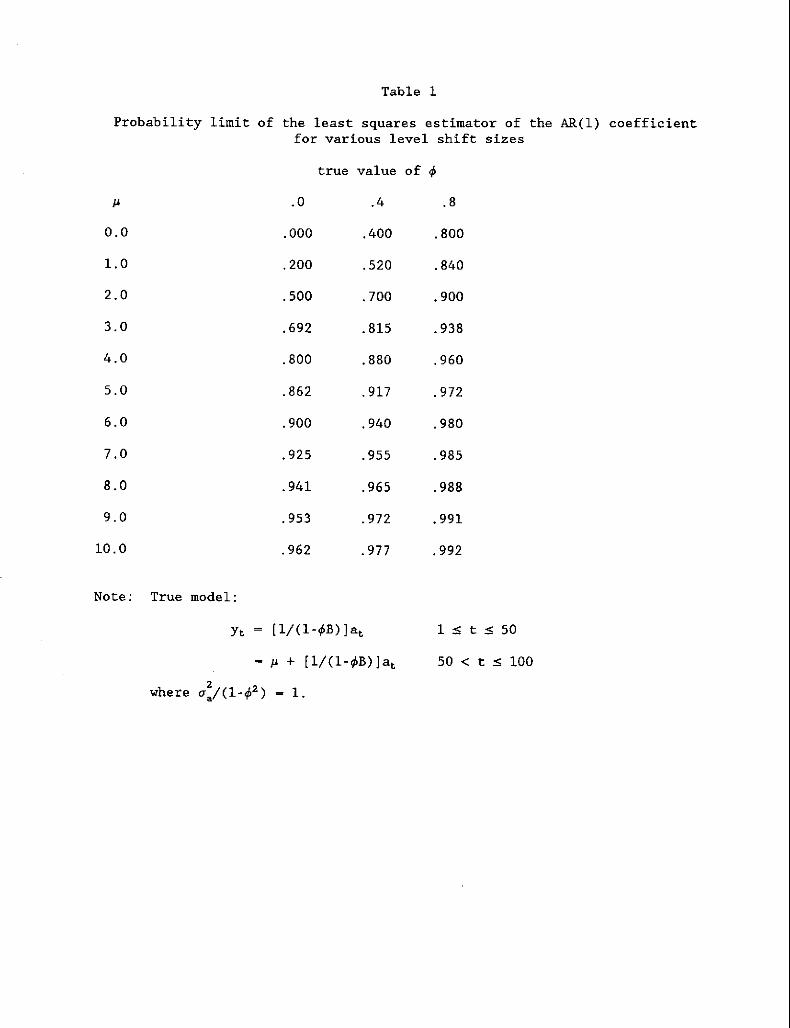
Table 1

Probability limit of the least squares estimator of the AR(l) coefficientfor various level shift sizes

true value of 1>

JJ .0 .4 .8

0.0 .000 .400 .800

1.0 .200 .520 .840

2.0 .500 .700 .900

3.0 .692 .815 .938

4.0 .800 .880 .960

5.0 .862 .917 .972

6.0 .900 .940 .980

7.0 .925 .955 .985

8.0 .941 .965 .988

9.0 .953 .972 .991

10.0 .962 .977 .992

Note: True model:

Yt - [l/(l-1>B) ]at loSt oS 50

- JJ + [l/(l-1>B) ]at 50 < t .:5 100

2where "./(1-1>2) - 1.

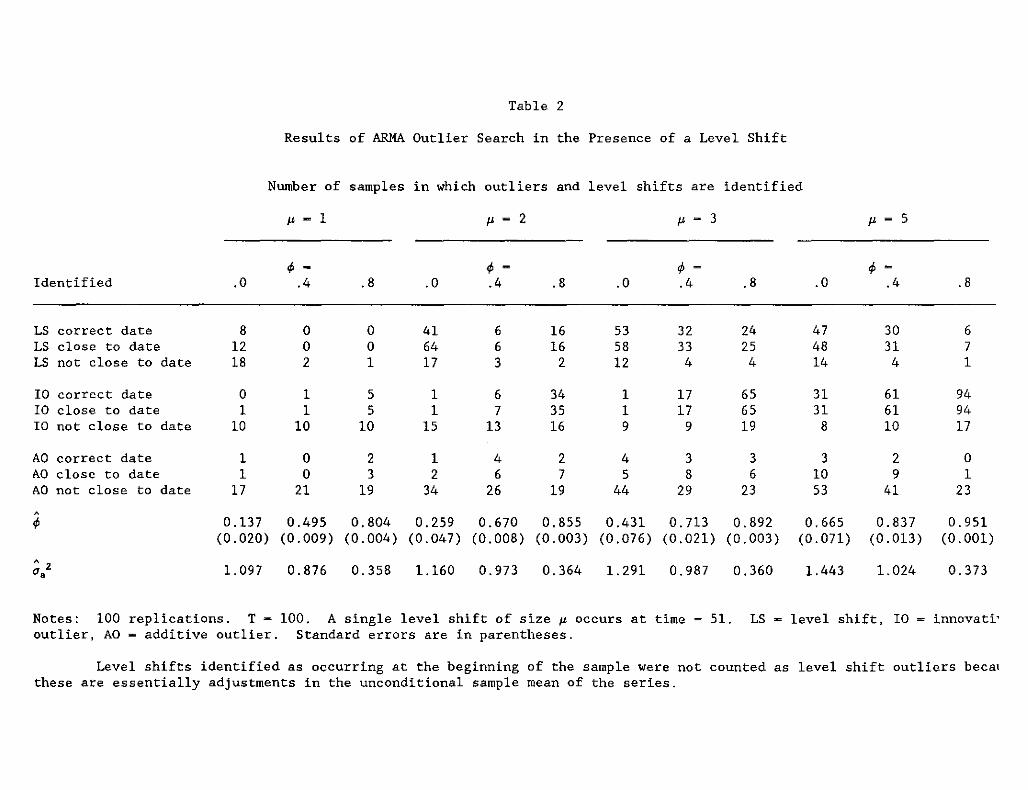
Table 2

Results of ARMA Outlier Search in the Presence of a Level Shift

Number of samples in which outliers and level shifts are identified

Jl - 1 Jl - 2 Jl - 3 Jl - 5

if> - if> - if> - if> -Identified .0 .4 .8 .0 .4 .8 .0 .4 .8 .0 .4 .8

LS correct date 8 0 0 41 6 16 53 32 24 47 30 6LS close to date 12 0 0 64 6 16 58 33 25 48 31 7LS not close to date 18 2 1 17 3 2 12 4 4 14 4 1

10 correct date 0 1 5 1 6 34 1 17 65 31 61 9410 close to date 1 1 5 1 7 35 1 17 65 31 61 9410 not close to date 10 10 10 15 13 16 9 9 19 8 10 17

AO correct date 1 0 2 1 4 2 4 3 3 3 2 0AO close to date 1 0 3 2 6 7 5 8 6 10 9 1AO not close to date 17 21 19 34 26 19 44 29 23 53 41 23A

if> 0.137 0.495 0.804 0.259 0.670 0.855 0.431 0.713 0.892 0.665 0.837 0.951(0.020) (0.009) (0.004) (0.047) (0.008) (0.003) (0.076) (0.021) (0.003) (0.071) (0.013) (0.001)

A 21. 097 0.876 0.358 1.160 0.973 0.364 1. 291 0.987 0.360 1.443 1.024 0.373u.

Notes: 100 replications. T - 100. A single level shift of size Jl occurs at time - 51. LS - level shift, 10 - innovativeoutlier, AO - additive outlier. Standard errors are in parentheses.

Level shifts identified as occurring at the beginning of the sample were not counted as level shift outliers becausethese are essentially adjustments in the unconditional sample mean of the series.

Table 3

Results of White Noise Outlier Search in the Presence of a Level Shift

Number of samples in which outliers and level shifts are identified

I" - 1 I" - 2 I" - 3 I" - 5

1> - 1> - 1> - 1> -Identified .0 .4 .8 .0 .4 .8 .0 .4 .8 .0 .4 .8

LS correct date 23 20 20 70 62 64 93 90 92 100 100 100LS close to date 45 37 39 99 94 87 100 100 99 100 100 100LS not close to date 33 52 75 36 57 87 29 58 87 31 55 86

10 correct date 0 1 5 0 3 11 0 3 19 0 5 2010 close to date 1 2 6 1 4 12 0 4 20 1 6 2110 not close to date 1 9 15 5 10 18 1 11 15 2 9 16

AO correct date 1 0 2 1 1 3 1 1 5 2 0 5AO close to date 1 0 4 1 5 6 1 4 10 4 3 8AO not close to date 27 28 29 30 33 29 25 28 10 29 30 26,1> 0.061 0.385 0.688 0.054 0.378 0.683 0.086 0.399 0.676 0.065 0.390 0.686

(0.012) (0.010) (0.008) (0.011) (0.013) (0.008) (0.010) (0.010) (0.009) (0.010) (0.009) (0.007)

~2 1.023 0.801 0.321 1.009 0.790 0.322 1.048 0.805 0.319 1.013 0.802 0.323•

Notes: 100 replications. T - 100. A single level shift of size I" occurs at time - 51. LSoutlier, AO - additive outlier. Standard errors are in parentheses.

level shift, 10 innovative

Level shifts identified as occurring at the beginning of the sample were not counted as level shift outliers becausethese are essentially adjustments in the unconditional sample mean of the series.

Data Set

123456 +78 +9

10 +111213 +14 +15161718 +19 +2021 +22 +­2324

Notes: +

Table 4

Final Intervention Model

Actual ARMA Outlier Search CR Outlier Search

A A

¢ Outliers ¢ Outliers ¢ Outliers

0.0 NONE 0.107 A097 0.107 A0970.0 LS55 0.0 LS55 0.0 LS550.0 A076 -0.170 A076 -0.170 A0760.0 A078 -0.120 I078,A079 -0.123 A078,A0790.0 LS58,A059 0.0 A058, LS60 . 0.0 A058,LS600.0 LS17,A029 0.702 NONE 0.0 LS180.0 A035,A04l 0.0 A035,A04l 0.0 A035,A04l0.0 LS23,A036,A038 0.813 A022,A038,A082 0.0 LS23,A0380.4 NONE 0.324 NONE 0.324 NONE0.4 LS48 0.920 1048 0.293 LS480.4 IOn 0.446 I03l,A052 0.446 I03l,A0520.4 A056 0.507 I037,A044,A056 0.507 I037,I044,A0560.4 I056,LS8l 0.181 A056,LS8l 0.255 I056,LS8l0.4 LS23,A06l 0.890 AOl3, I023 ,A06l 0.272 LS23,A06l0.4 I018,A052 0.419 I018,A052 0.419 I018,A0520.4 AOll, LS44, 1078 0.246 AOll,LS44,A078 0.246 AOll,LS44,A0780.8 NONE 0.753 NONE 0.688 LS9l0.8 LS59 0.964 1059 O. n4 LS590.8 1087 0.784 1087 0.784 10870.8 A057 0.885 I049,A057 0.885 I049,A0570.8 LS28 ,IOn 0.942 I029,I03l,LS59,I087,A096 0.747 LS28,I03l,I087,A0960.8 LS59,Aon 0.985 I059,Aon 0.826 109, LS59 ,Aon0.8 I028,A045 0.794 I028,A045 ,1099 0.794 1028 ,A045, 10990.8 I034,A055,LS72 0.796 I034,I047,A055,LS72 0.796 I034.I047,A055,LS72

indicates an improvement in model specification when using combine/reduce outlier search asopposed to the ARMA outlier search.indicates a spurious outlier or level shift was introduced by the combine outlier search.

AO## indicates an additive outlier in time period ##, 10## indicates an innovative outlier intime period ##, and LS## indicates a level shift in time period ##.

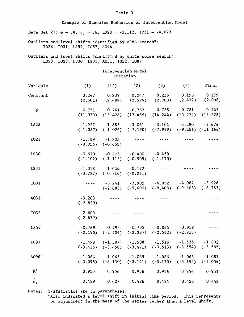
Table 5

Example of Stepwise Reduction of Intervention Model

Data Set 21: ¢ ~ .8, u, - .6, LS28 ~ -3.112, 1031 - -4.073

Outliers and level shifts identified by ARMA search':1028, 1031, LS59, 1087, A096

Outliers and level shifts identified by white noise search':LS28, 1028, LS30, LS31, A031, 1032, 1087

Intervention ModelIteration

Variable

Constant

(1)

0.247(2.501)

0.751(11.939)

(1')

0.239(2.489)

0.761(13.426)

(2)

0.247(2.594)

0.762(13.486)

(3)

0.236(2.703)

0.768(14.244)

(4)

0.196(2.477)

0.781(15.272)

Final

0.179(2.098)

0.747(13.228)

LS28

1028

-1. 927(-1.087)

-1.189(-0.056)

-1.885(-1.026)

-1. 233(-0.658)

-3.061(-7.190)

-3.104(-7.999)

-3.290 -3.674(-9.286) (-11.166)

LS30 -0.670 -0.673 -0.400 -0.450(-1.102) (-1.113) (-0.905) (-1.170)

LS31

1031

A031

1032

LS59

-1. 018(-0.727)

-3.263(-2.829)

-2.603(-2.639)

-0.769(-2.195)

-1.044(-0.714)

-3.241(-2.683)

-0.792(-2.226)

-0.172(-0.261)

-3.905(-5.600)

-0.795(-2.237)

-4.052(-9.403)

-0.844(-2.562)

-4.087(-9.503)

-0.958(-2.913)

-3.928(-8.783)

1087

A096

ttl

-1.498(-3.415)

-1. 064(-3.096)

0.955

(-1.507) -1.508(-3.458) (-3.471)

-1.065 -1.065(-3.130) (-3.141)

0.956 0.956

-1. 516(-3.513)

-1. 066(-3.170)

0.956

-1. 535(-3.554)

-1.068(-3.192)

0.956

-1. 602(-3.585)

-1. 081(-3.054)

0.953

0.429 0.427 0.426 0.424 0.425 0.442

Notes: T-statistics are in parentheses.'Also indicated a level shift in initial time period. This represents

on adjustment in the mean of the series rather than a level shift.

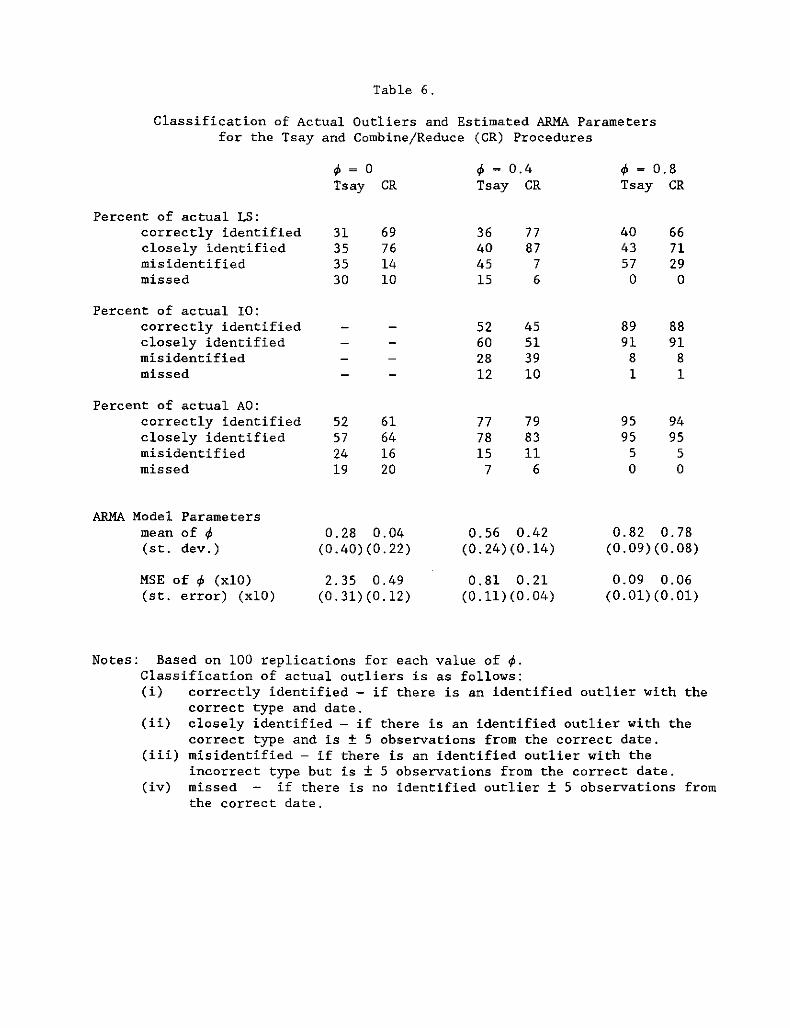
Table 6.

Classification of Actual Outliers and Estimated ARMA Parametersfor the Tsay and Combine/Reduce (CR) Procedures

4> - 0 4> - 0.4 4> - 0.8Tsay CR Tsay CR Tsay CR

Percent of actual LS:correctly identified 31 69 36 77 40 66closely identified 35 76 40 87 43 71misidentified 35 14 45 7 57 29missed 30 10 15 6 0 0

Percent of actual 10:correctly identified 52 45 89 88closely identified 60 51 91 91misidentified 28 39 8 8missed 12 10 1 1

Percent of actual AO:correctly identified 52 61 77 79 95 94closely identified 57 64 78 83 95 95misidentified 24 16 15 11 5 5missed 19 20 7 6 0 0

ARMA Model Parametersmean of 4> 0.28 0.04 0.56 0.42 0.82 0.78(st. dev. ) (0.40)(0.22) (0.24)(0.14) (0.09)(0.08)

MSE of 4> (xlO) 2.35 0.49 0.81 0.21 0.09 0.06(st. error) (xlO) (0.31)(0.12) (0.11)(0.04) (0.01)(0.01)

Notes: Based on 100 replications for each value of 4>.Classification of actual outliers is as follows:(i) correctly identified - if there is an identified outlier with the

correct type and date.(ii) closely identified - if there is an identified outlier with the

correct type and is ± 5 observations from the correct date.(iii) misidentified - if there is an identified outlier with the

incorrect type but is ± 5 observations from the correct date.(iv) missed if there is no identified outlier ± 5 observations from

the correct date.

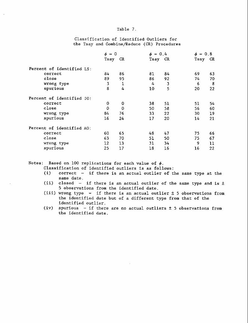
Table 7.

Classification of Identified Outliers forthe Tsay and Combine/Reduce (CR) Procedures

4> ~ a 4> ~ 0.4 4> ~ 0.8Tsay CR Tsay CR Tsay CR

Percent of identified LS:correct 84 86 81 84 69 63close 89 95 86 92 74 70wrong type 3 1 4 3 6 8spurious 8 4 10 5 20 22

Percent of identified 10:correct a a 38 51 51 54close a a 50 58 56 60wrong type 84 76 33 22 30 19spurious 16 24 17 20 14 21

Percent of identified AO:correct 60 65 48 47 75 66close 63 70 51 50 75 67wrong type 12 13 31 34 9 11spurious 25 17 18 16 16 22

same type at the

replications for each value of 4>.of identified outliers is as follows:

if there is an actual outlier of thecorrectsame date.closed if there is an actual outlier of the same type and is ±5 observations from the identified date.wrong type if there is an actual outlier ± 5 observations fromthe identified date but of a different type from that of theidentified outlier.spurious - if there are no actual outliers ± 5 observations fromthe identified date.

(ii)

(iii)

(iv)

Notes: Based on 100Classification( i)

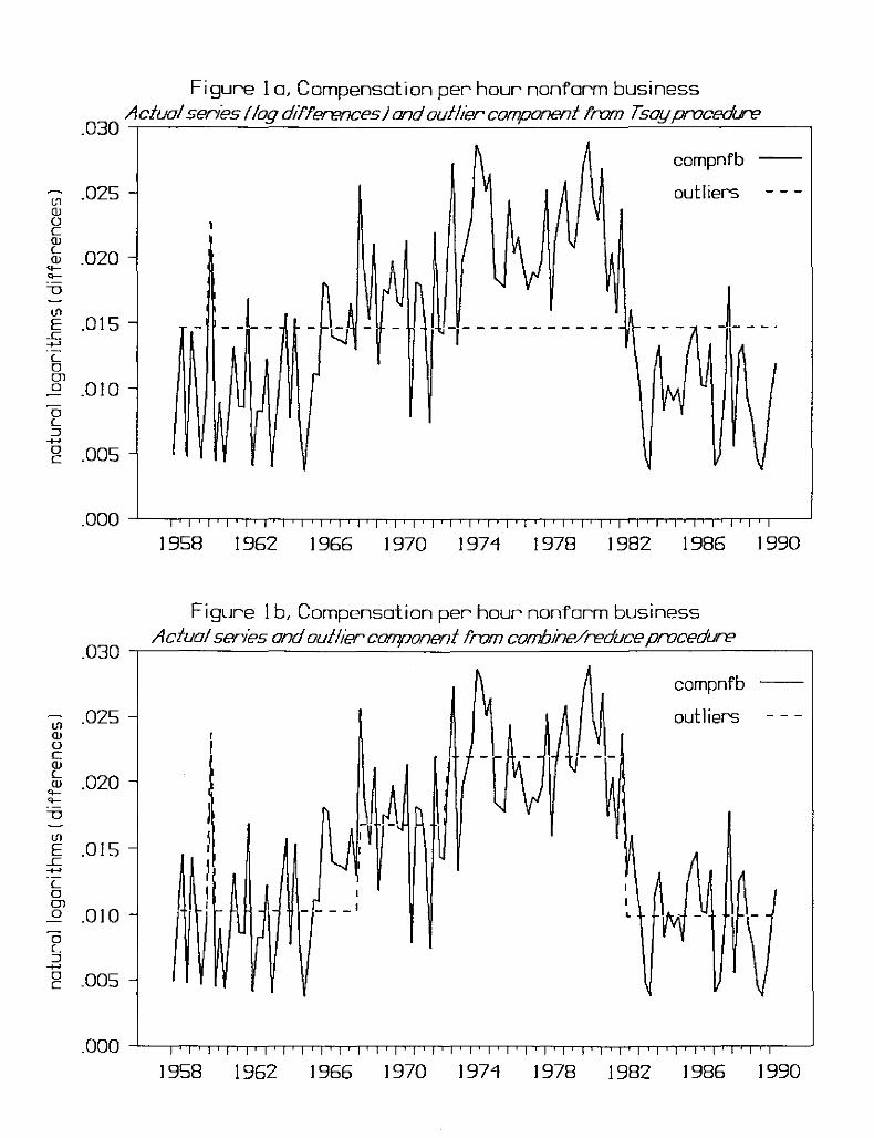
Figure 1a, Compensation per hour nonfarm businessActualseries Ilag dtfferences) andautlier component from Tsayprocedure

.030 --,-------=---------~---------''''-'----------,

co .025OJocOJLOJ .020'l­'l-

Ll

l!lE .015

..c+-'

Lo01o .010oL:::J

+-'

g .005

- --'-- - Q - - -r----------

compnfb

outliers

1958 1962 1966 1970 1974 1978 I 982 1986 1990

Figure 1b, Compensation per hour nonfarm businessActualseries andoutlier component from combine/reduceprocedure

.030 --,-------------'--------------'---------,

LO .025OJocOJL~ .020'l­

Ll

coE .015

..c+-'

Lo01o .010oL:::J

+-'

~ .005 I

lllII

~---'

compnfb

outliers

L

1958 1962 1966 1970 197"1 1978 1982 1986 1990

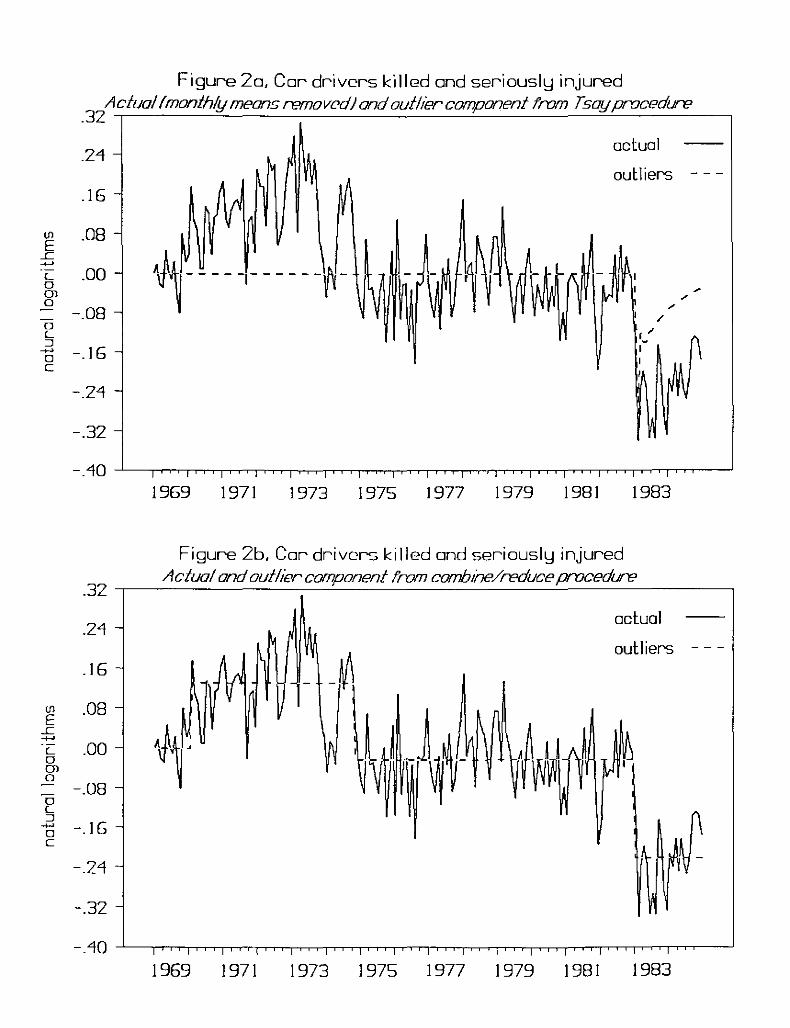
Figure 20, Cor drivers killed and seriousl\d injuredActual(monthly means removed) ondoutlIer component from Tsayprvcedure

.32 ,-----=------,--------'--------=--=---------,

.24 -

W~.16 -

It.08 -co

E

~~- - - - -,- - - - - -~-L-+-'

L .00 - --1 -0 , I"010

-.08 -0L:::J

-+-" -.16 -0c

-.24 -

-.32 -

actual

outliers

1969 1971 1973 1975 1977 1979 1981 1983

Figure 2b. Car drivers killed and seriousl\d injuredActualandoutlier component frvm combine/reduceprvcedure

.32 ,----------,--'-------------'-----------,

.24

.16

co .08E

L-+-'

L .00o01o

-.08oL:::Jo -.16c

-.24

-.32

actual

outliers

1969 1971 1973 1975 1977 1979 1981 1983

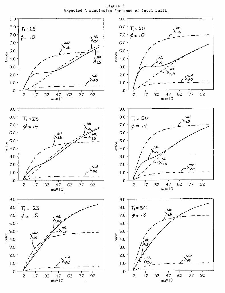
Figure 3Expected A statistics for case of level shift

,,/

//

I 7 32 47 62 77 92mu*IO

2

1";:: 50

f;= .0

9.0,----------------,

8.0

7.0

60

.g 5.0

] 4.0

3.0

20

1.0

.0 -l-'F-,----,r---r-~-__r-_r---lI7 32 47 62 77 92

mu* I0

""- - -

2

90,----------------,

8.0

7.0

6.0

5.0.g

140

-----

9.0

8.0 T, ::: 50 wzJ),.<-5

7.0~= .1 _.L------

.--6.0 ,,/

0 5 .0/

"I

140 ,.3.0 /

/ M.

2.0 / /~).IO w/J

/ ..c~""_1.0 / -/ - -0

tV'

2 17 32 47 62 77 92mu*IO

- - - - -

2 17 32 47 62 77 92mu*IO

9.0 r-----------------,

8.0

7.0

6.0

.g 5.0

1 4.0

3.0

2.0

1.0

.0 -'---r,==-r------,r---r-~-__r-___,---l

9.0

8.0 1";::: 2S7.0 rf: .'8 All

AID..6.0 L" NO!·50

:~/. ~LS ----c ---" / - --

140~

\~/3.0

2.0 It"/" ..,OJ

1.0 I L~A~- - - - - -0

2 17 32 47 62 77 92mu*10

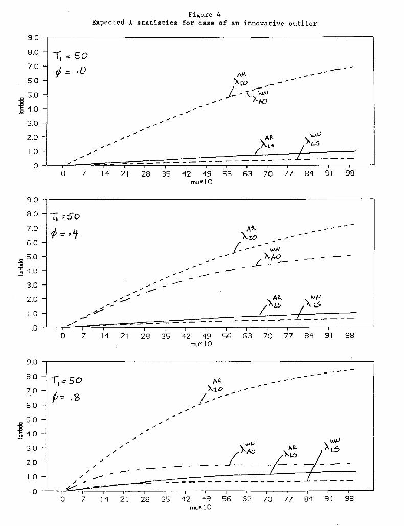
Figure 4Expected A statistics for case of an innovative outlier

9.0

8.0 - -r; =: 507.0 - ¢: ·0 -- --AI< ---6.0 - '>-:tD --,---

50 - 1- - -\.--~(Jo . _ - - Af(J-0

14.0 - -.;-3.0 - ------ "vJrJ2.0 - - -;P-- / "'l..-S-,; LS-1.0 - - f- _:L,;.;

0 -0 7 14 21 28 35 42 49 56 63 70 77 84 91 98

mu"10

9.0

8.0 - I;=:S-O7.0 - A~ ---

¢::·If \..06.0 - f ----;;50 - -- AltO - - -

0 - _.-£.-- --0

:i 4.0 - - -,; - --- -3.0 - ----2.0 - -- '>tr- "'(oJ-::.--- /~LS-- / L51.0 - ~- _.1....-

.0 /' -. -. , ,0 7 14 21 28 35 42 49 56 63 70 77 84 91 98

mu"10

,; --,; - ---- --- --- ---

Appendix for

Detecting Level Shifts in Time Series:

Misspecification and a Proposed Solution

Nathan S. Balke

Assistant Professor of EconomicsSouthern Methodist University

and

Research AssociateFederal Reserve Bank of Dallas

1

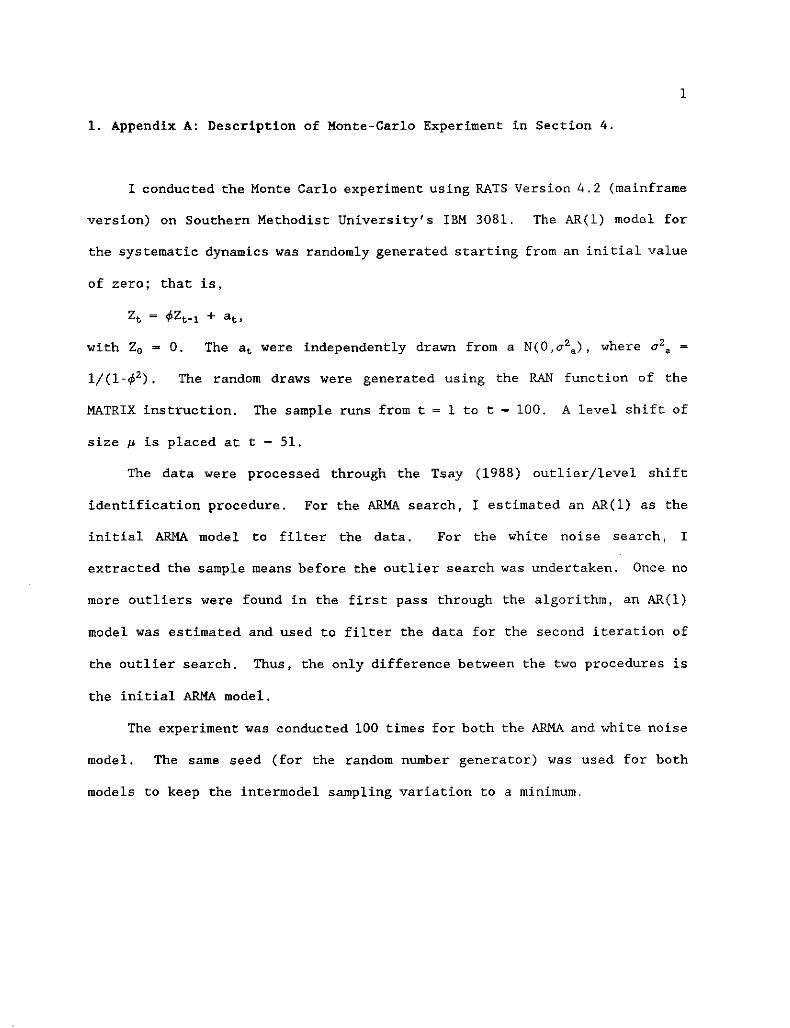
1. Appendix A: Description of Honte-Carlo Experiment in Section 4.

I conducted the Monte Carlo experiment using RATS Version 4.2 (mainframe

version) on Southern Methodist University's IBM 3081. The AR(l) model for

the systematic dynamics was randomly generated starting from an initial value

of zero; that is,

Zt - qlZt-l + at,

wi th Zo O. The at were independently drawn from a N(0, a 2a), where a 2a -

1/(1-ql2) . The random draws were generated using the RAN function of the

MATRIX instruction. The sample runs from t - 1 to t - 100. A level shift of

size p is placed at t - 51.

The data were processed through the Tsay (1988) outlier/level shift

identification procedure. For the ARMA search, I estimated an AR(l) as the

initial ARMA model to filter the data. For the white noise search, I

extracted the sample means before the outlier search was undertaken. Once no

more outliers were found in the first pass through the algorithm, an AR(l)

model was estimated and used to filter the data for the second iteration of

the outlier search. Thus, the only difference between the two procedures is

the initial ARMA model.

The experiment was conducted 100 times for both the ARMA and white noise

model. The same seed (for the random number generator) was used for both

models to keep the intermodel sampling variation to a minimum.

2

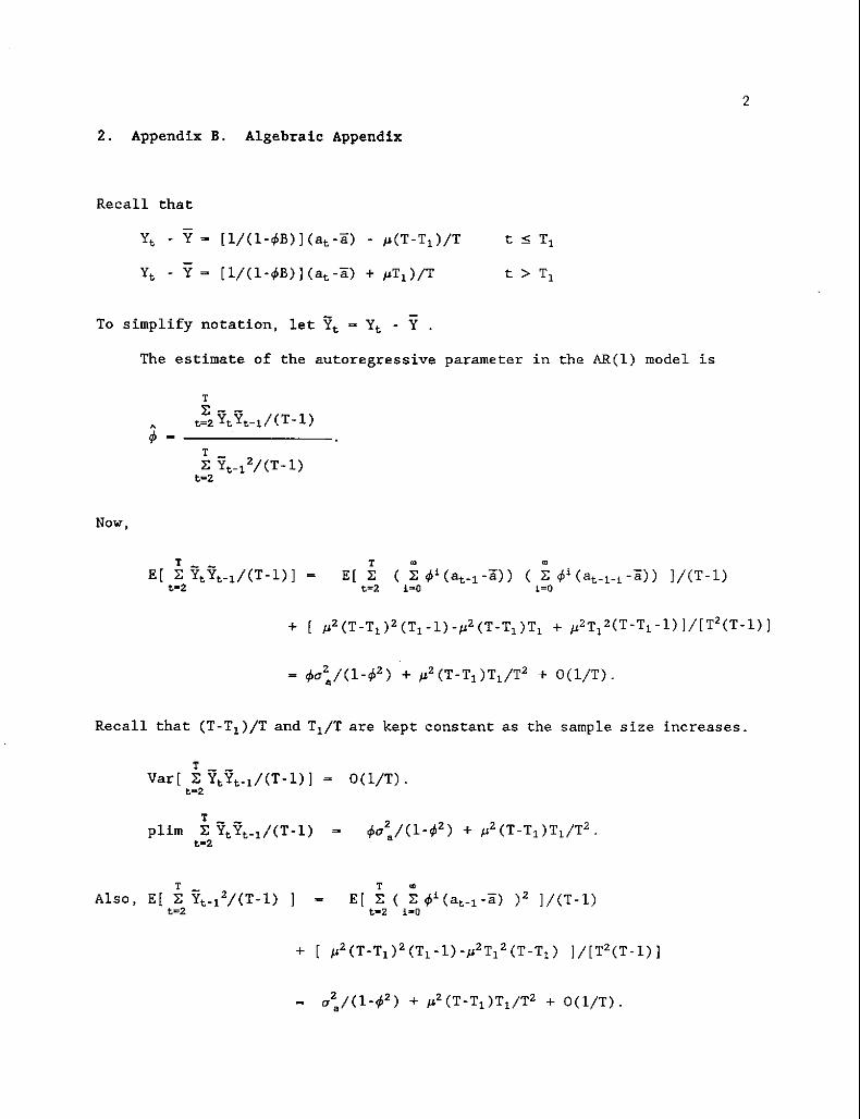
2. Appendix B. Algebraic Appendix

Recall that

Y - [l/(l-4>B) J(at -a) - p(T-T, )/T

Yt - Y - [l/(l-4>B)](at -a) + pT,)/T

To simplify notation, let Yt - Yt - Y

t :5 T,

t > T,

Now,

The estimate of the autoregressive parameter in the AR(l) model is

TE[ :1;

t-2

~ ~

( :1; 4>' (at-l -a» ( :1; 4>' (at-l-i -a» J1(T-l)i-O i=O

Recall that (T-T,)/T and T,/T are kept constant as the sample size increases.

T _ _

Var[ :1; Yt Yt -l /(T-1)] - O(l/T).t-2

T __

plim :1; Yt Yt-,! (T -1)t=2

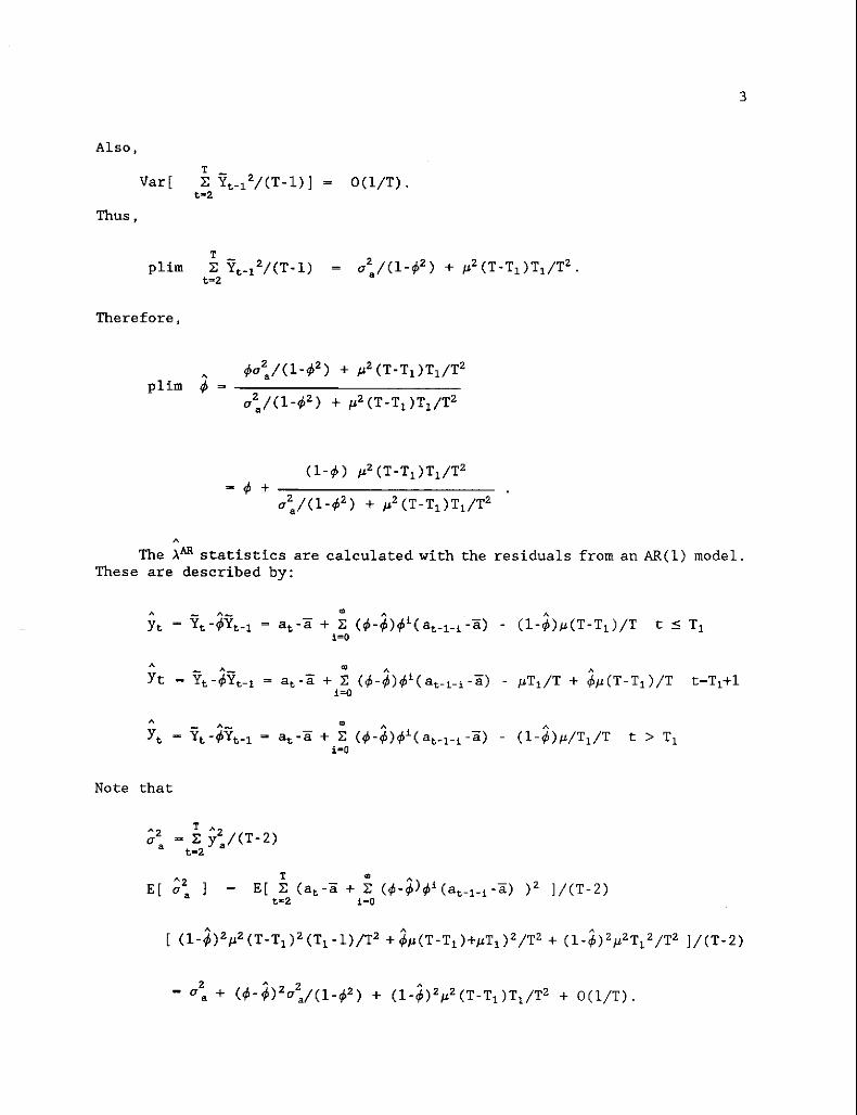
T - 2Also, E[ :1; Yt -l I(T-1)t-2

T ~

E[:1; (:1;4>i(at_l-a) )2 J/(T-1)t-2 i-O

3

Also,T _

Var[ ~ y t _12/(T-l)] - G(l/T).t-2

Thus,

Tplim ~ 'i\_12/(T-l)

t-2

Therefore,

plim

(l-¢) ~2(T-Tl)Tl/T2

- ¢ + -----------a:/(1-¢2) + ~2(T-Tl)Tl/T2

A

The liAR statistics are calculated with the residuals from an AR(l) model.These are described by:

A A_ m A ,Yt - 'It -¢Yt - l - at- a + ~ (¢-¢)¢ (at-l-i -a)

i=O

A A_ m AYt - 'It -¢Yt - l - at-a + L: (¢-¢)¢'( at-l-i -a)

i=O

A A_ m

(¢_¢)¢i( at-l-i -a)Yt - 'It -¢Yt - l - at -a + ~

i-O

Note that

A2 T A2a. - ~ y./(T-2)

t-2

A

~Tl/T + ¢~(T-Tl)/T t-Tl+l

A

(l-¢)~/Tl/T t > Tl

A2E [ a. J

A A A

[ (1_¢)2~2 (T-Tl )2 (Tl -1)/T2 + ¢~(T-Tl )+~T,)2 /T2 + (1_¢)2~2T12 /T2 JI(T-2)

Also,

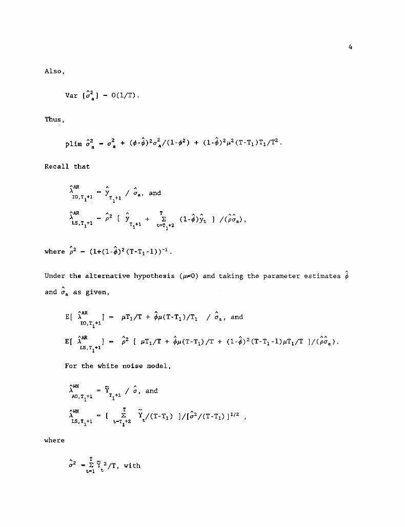
'2Var [a.] - O(l/T).

Thus,

4

plim ~~

Recall that

'AR , ,,\ - Y I a., andIO,T

1+1 T

1+1

'AR ;2 , T , , AA,\ [ Y + }; (l-.p)Yt I(pa.) ,LS , T!+1 T

1+1 t=T

1+2

,Under the alternative hypothesis (~~O) and taking the parameter estimates'll

and ua as given,

, ,~TI/T + .p~(T-Tl)/Tl I a., and

For the white noise model,

,I a, and

where

T};

t-T1+2

, T _a2 _ }; y 2 IT, with

t-l t

5

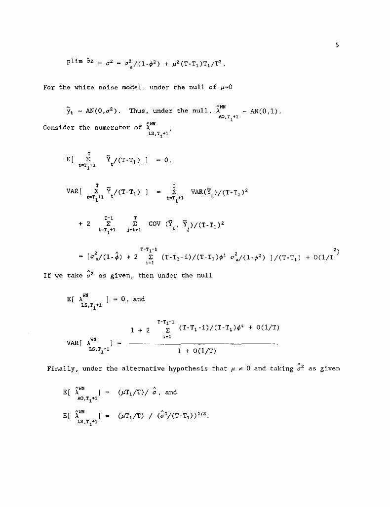
plim 02

For the white noise model, under the null of ~~O

Consider the numerator of

Yt - AN(O,,,2). Thus, under the null,

- O.

VAR[T:E

t"T1+l

T

:E COV (Y , Y)/(T-T, )2j=t+l t j

2 A T-T1-l

- ["./(l-~) + 2 :E1;1

If we takeA

2" as given, then under the null

I + 2 (T-T,-i)/(T-T,)~i + O(l/T)

VAR[I + O(l/T)

A2Finally, under the alternative hypothesis that ~ ~ 0 and taking" as given

AWN AE[ A J (~TtlT)/ ", and

AO,T1+1

E[AWN

J (~TtlT) / (;2/(T-T, » 112.ALS.T 1+1

RESEARCH PAPERS OF THE RESEARCH DEPARTMENTFEDERAL RESERVE BANK OF DALLAS

Available, at no charge, from the Research DepartmentFederal Reserve Bank of Dallas, Station K

Dallas, Texas 75222

9001

9002

9003

9004

9005

Another Look at the Credit-Output Link (Cara S. Lown and Donald W.Hayes)

Demographics and the Foreign Indebtedness of the United States (JohnK. Hill)

Inflation, Real Interest Rates, and the Fisher Equation Since 1983(Kenneth M. Emery)

Banking Reform (Gerald P. O'Driscoll, Jr.)

U.S. Oil Demand and Conservation (S.P.A. Brown and Keith R. Phillips)

9006 Are Net Discount Ratios Stationary?:Value Calculations (Joseph H. Haslag,Slottje)

The Implications for PresentMichael Nieswiadomy and D.J.

9007 The Aggregate Effects of Temporary Government Purchases (Mark A.Wynne)

9008 Lender of Last Resort: A Contemporary Perspective (George G. Kaufman)

9009 Does It Matter How Monetary Policy is Implemented? (Joseph H. Haslagand Scott E. Hein)

9010 The Impact of Differential Human Capital Stocks on Club Allocations(Lori L. Taylor)

9011 Is Increased Price Flexibility Stabilizing? The Role of the PermanentIncome Hypothesis (Evan F. Koenig)

9012 Fisher Effects and Central Bank Independence (Kenneth M. Emery)

9013 Methanol as an Alternative Fuel (Mine K. Yucel)

9101 Large Shocks, Small Shocks, and Economic Fluctuations: Outliers inMacroeconomic Time Series (Nathan S. Balke and Thomas B. Fomby)

9102 Immigrant Links to the Home Country: Empirical Implications for U.S.and Canadian Bilateral Trade Flows (David M. Gould)

9103 Government Purchases and Real Wages (Mark Wynne)

9104 Evaluating Monetary Base Targeting Rules (R.W. Hafer, Joseph H. Haslagand Scott E. Hein)

9105 Variations in Texas School Quality (Lori L. Taylor and Beverly J. Fox)

9106 What Motivates Oil Producers?: Testing Alternative Hypotheses (CarolDahl and Mine Yucel)

9107 Hyperinflation, and Internal Debt Repudiation in Argentina and Brazil:From Expectations Management to the "Bonex" and "CallarI! Plans (JohnH. Welch)

9108 Learning From One Another: The U.S. and European Banking Experience(Robert T. Clair and Gerald P. O'Driscoll)

9109 Detecting Level Shifts in Time Series: Misspecification and aProposed Solution (Nathan S. Balke)