Embed Size (px)
Citation preview
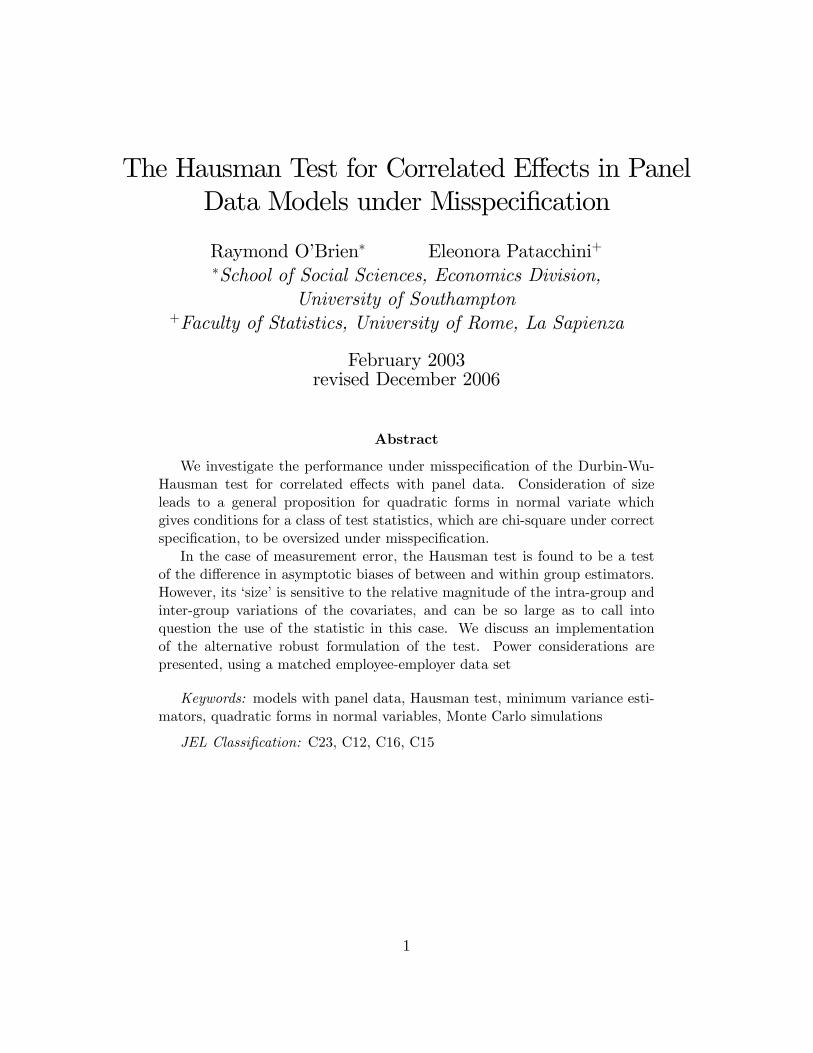
The Hausman Test for Correlated E¤ects in PanelData Models under Misspeci�cation
Raymond O�Brien� Eleonora Patacchini+�School of Social Sciences, Economics Division,
University of Southampton+Faculty of Statistics, University of Rome, La Sapienza
February 2003revised December 2006
Abstract
We investigate the performance under misspeci�cation of the Durbin-Wu-Hausman test for correlated e¤ects with panel data. Consideration of sizeleads to a general proposition for quadratic forms in normal variate whichgives conditions for a class of test statistics, which are chi-square under correctspeci�cation, to be oversized under misspeci�cation.In the case of measurement error, the Hausman test is found to be a test
of the di¤erence in asymptotic biases of between and within group estimators.However, its �size�is sensitive to the relative magnitude of the intra-group andinter-group variations of the covariates, and can be so large as to call intoquestion the use of the statistic in this case. We discuss an implementationof the alternative robust formulation of the test. Power considerations arepresented, using a matched employee-employer data set
Keywords: models with panel data, Hausman test, minimum variance esti-mators, quadratic forms in normal variables, Monte Carlo simulations
JEL Classi�cation: C23, C12, C16, C15
1

1 Introduction
The Hausman test is the standard procedure used in empirical panel data analysisin order to discriminate between the �xed e¤ects and random e¤ects model. 1 Thegeneral set up can be described as follows. Suppose that we have two estimators fora certain parameter � of dimension K � 1: One of them , b�r, is robust, i.e. consistentunder both the null hypothesis H0 and the alternative H1, the other, b�e; is e¢ cientand consistent under H0 but inconsistent under H1: The di¤erence between the twois then used as the basis for testing. Hausman, (1978) shows that, under appropriate
assumptions, under H0 the statistic h based on�b�R � b�E� has a limiting chi-squared
distribution:
h =�b�r � b�e�0 hdV ar �b�r � b�e�i�1 �b�r � b�e� a� �2K :
If this statistic lies in the upper tail of the chi-square distribution we reject H0: Ifthe variance matrix is consistently estimated, the test will have power against anyalternative under which b�r is robust and b�e is not. Holly (1982) discusses the powerin the context of maximum likelihood.Hausman also shows that, again under appropriate assumptions,
V ar�b�r � b�e� = V ar �b�r�� V ar �b�e�
It is well known that the assumptions used are su¢ cient but not necessary, as dis-cussed in Ruud (2000), or Wooldridge (1995, 2002), or Newey and McFadden (1994).
Further, while it may be convenient to estimate V ar�b�r � b�e� using this result, one
can argue that using
V ar�b�r � b�e� = V ar �b�r�� 2Cov �b�r;b�e�+ (V ar �b�e�
may be more robust, and the trade-o¤ between robustness and power should beconsidered.The plan of the paper is as follows. Section 2 presents a robust formulation of the
Hausman test for correlated e¤ects, which is based on the construction of an auxiliaryregression. We explain and discuss to what extent the use of arti�cial regressions mayallow us to construct tests based on the di¤erence between two estimators in a paneldata model without making strong assumptions about the disturbances. The motiva-tion underlying the implementation of the robust test is that the size distortion of thestandard Hausman test in cases of misspeci�cation of the variance-covariance matrixof the disturbances may be serious. This is investigated in Section 3. We formulate
1This approach is also used by Durbin (1954) and Wu (1973). For this reason tests based on thecomparison of two sets of parameter estimates are also called Durbin-Wu-Hausman tests, or DWH.For simplicity of exposition we will refer to the Hausman (1978) set up.
2
a general proposition for positive-de�nite quadratic forms in normal variate whichgives conditions for a class of test statistics, which are chi-square under correct spec-i�cation, to be oversized under misspeci�cation. We then investigate measurementerror in panels.Section 4 compares the power of the standard Hausman test and the robust formu-
lation presented in Section 2 using a Monte Carlo experiment. Section 5 concludes.
2 A robust test by arti�cial regression
Consider the model
yit = x0
it� + �i + vit; i = 1; :::; N; t = 1; :::; T (1)
where xit is a K � 1 vector of stochastic regressors, �i � iid�0; �2�
�; vit � iid (0; �2)
are uncorrelated with xit and Cov (�i; vit) = 0:De�ning the disturbance term
"it = �i + vit;
the variance-covariance matrix of the errors is
�(NT�NT )
= IN
where
=
0B@ �2� + �2 : : : �2�
.... . .
...�2� : : : �2� + �
2
1CA = �2IT + �2� ��
0(2)
and � is a column vector of T ones.The unobserved heterogeneity implies correlation over time for single units, but
there is no correlation across units.Hausman and Taylor (1981) propose three di¤erent speci�cation tests for the null
hypothesis of uncorrelated e¤ects: one based on the di¤erence between the WithinGroups and the Balestra-Nerlove estimator, another on the di¤erence between theBalestra-Nerlove and the Between Groups and a third on the di¤erence between theWithin Groups and the Between Groups. They show that the chi-square statisticsfor the three tests are numerically identical. We now analyze the Hausman statisticconstructed on the di¤erence between the Within Groups and the Balestra-Nerloveestimator, commonly used in empirical work.Let
� =�2
�2 + T�2�:
We write the Balestra-Nerlove estimator (Balestra and Nerlove, 1966) as a functionof the variables in levelsb�BN = �X 0
QX + �X0MX
��1 �X
0Q+ �X
0M�Y (3)
3
where
Q = IN Q+;
Q+ = IT �1
Tii0;
M = IN M+;
M+ =1
Tii0= IT �Q+;
X =
26664X1
X2...XN
37775 ; Y =26664y1y2...yN
37775 ; Xi =
26664x0i1x0i2...x0iT
37775 ; yi =26664yi1yi2...yiT
37775 :Q+ is the matrix that transforms the data to deviations from the individual timemean, M+ is the matrix that transforms the data to averages. Rearranging
b�BN = hX 0[�INT + (1� �)Q]X
i�1X
0[�INT + (1� �)Q]Y: (4)
The variance is
V ar(b�BN) = �2 hX 0[�INT + (1� �)Q]X
i�1: (5)
Similarly, using the Q matrix de�ned in formula (3), we write also theWithin Groupsestimator as a function of the initial variables in levels
b�WG =hX
0QX
i�1X
0QY: (6)
The variance isV ar(b�WG) = �
2hX
0QX
i�1: (7)
Also,Cov(b�BN ; b�WG) = V ar(
b�BN):This is symmetric, and thus equal to Cov(b�WG; b�BN). Therefore, we obtain
V ar(b�BN � b�WG) = V ar(b�WG)� V ar(b�BN):The equality (??) holds for � known or otherwise �xed.As we said, the case of estimated � can be treated by using the Hausman-Taylor
result that an algebraically identical test statistic can be constructed using the dif-ference between b�WG and the Between Groups estimator b�BG: We obtain
(b�WG � b�BG)0 hV ar(b�WG) + V ar(b�BG)i�1 (b�WG � b�BG)
4
as the estimators have zero covariance when we de�ne the Between Groups estimatoras usual: b�BG = �X 0
MX��1
X0MY
V ar(b�BG) = �2(1 + �T ) hX 0MX
i�1; � = �2�=�
2: (8)
In this form, we can see that estimating �2 and � (or �2�) a¤ects only the variancematrix of the test statistic.A robust version of the Hausman test can be based on the use of an arti�cial
regression. We estimate directly the variance of the di¤erence of the two estimators.Moreover, this provides an estimate for this variance that is consistent and robustto heteroscedasticity and/or serial correlation of arbitrary form in the within groupscovariance matrix of the random disturbances. These estimators are obtained usingWhite�s formulae (White, 1984). It will be made clear to what extent the applicationof White�s heteroscedasticity consistent estimators of covariance matrices in a paneldata framework may also allow for the presence of dynamic e¤ects within groups.Di¤erent arti�cial regressions have been proposed in the panel data literature to
test for the presence of random individual e¤ects, such as a Gauss-Newton regressionby Baltagi (1996) or that proposed by Ahn and Lo (1996). However, the assumptionof initial spherical disturbances has not been relaxed. As shown by Baltagi (1997,1998), under the assumption of spherical disturbances, the three approaches, i.e. theHausman speci�cation test, the Gauss-Newton regression and the regression proposedby Ahn and Lo, yield exactly the same test statistic. Arellano (1993) �rst noted in thesame panel data framework that an auxiliary regression can also be used to obtain ageneralized test for correlated e¤ects which is robust to heteroscedasticity and corre-lation of arbitrary forms in the disturbances. Davidson and MacKinnon (1993) list atleast �ve di¤erent uses for arti�cial regressions including the calculation of estimatedcovariances matrices. We will use this device to estimate directly the variance be-tween the two estimators without using equality (??). Furthermore, the applicationof White�s formulae (White, 1984) in the panel data case will lead to heteroscedastic-ity and autocorrelation consistent estimators of such variance. Therefore, we can usean arti�cial regression to construct a test for the comparison of di¤erent estimatorswhich is robust to deviations from the assumption of spherical disturbances. Fromnow on we will call this technique the HR-test, for Hausman-Robust test.Next we present the auxiliary regression that was proposed by Arellano (1993) to
test for random versus �xed e¤ects in a static panel data model.Consider the general panel data model for individual i
yi(T�1)
= Xi(T�K)
� + vi(T�1)
; i = 1; :::; N:
This system of T equations in levels can be transformed into (T � 1) equations in
5
deviations and one in averages. We obtain�y�i = x
�i� + �
�i �! (T � 1) equations
yi = xi� + �i �! 1 equation.
Estimating by OLS the N(T � 1) equations in orthogonal deviations from individualtime-means we obtain the Within Groups estimator, i.e. b�WG: Estimating by OLSthe N average equations we obtain the Between Groups estimator, i.e. b�BG:Let
�WG = E�b�WG
�and
�BG = E�b�BG� :
Rewrite the system as�y�i = x
�i�WG + �
�i � x�i�BG + x�i�BG
yi = xi�BG + �i:
Rearranging, we obtain�yi = x
�i (�WG � �BG) + x�i�BG + ��i
yi = xi�BG + �i:
Call
Y +i =
�y�iyi
�;W+
i =
�x�i x�i0 xi
�;
�+ =
��1�2
�=
��WG � �BG
�BG
�; �+i =
���i�i
�:
The augmented auxiliary model is
Y +i = W+i �
+ + �+i ; i = 1; :::; N: (9)
If we estimate �+ by OLS, we obtain directly the variance of the di¤erence of thetwo estimators in the upper left part of the variance-covariance matrix of �+: If wethen estimate this covariance matrix using the White�s formulae and we perform aWald test on appropriate coe¢ cients, we obtain a reliable HR-test comparing the twoestimators we are interested in, namely b�WG and b�BG. As �rst noted by Arellano(1993), under the assumption of spherical disturbances a Wald test on appropriatecoe¢ cients in the auxiliary regressions is equivalent to the standard Hausman test.Appendix 1 provides an analytical derivation of the result below.Let
H+ =1
Ti0; H = IN H+; H 0H =
1
TMb�BG = [(HX)0(HX)]�1(HX)0(HY ) = (X 0MX)�1X 0MYb�WG = [(QX)0(QX)]�1(QX)0(QY ) = (X 0QX)�1X 0QY
6
Further, let G+ be Arellano and Bover�s (1990) forward orthogonal deviations matrix,(T � 1)� T; such that
G+i = 0; G+G+0= I(T�1); G
+0G+ = Q+ = IT �1
Tii0
G = IN G+; G0G = Q;GG0 = IN I(T�1) = IN(T�1)b�WG = [(GX)0(GX)]�1(GX)0(GY ) = (X 0QX)�1X 0QY
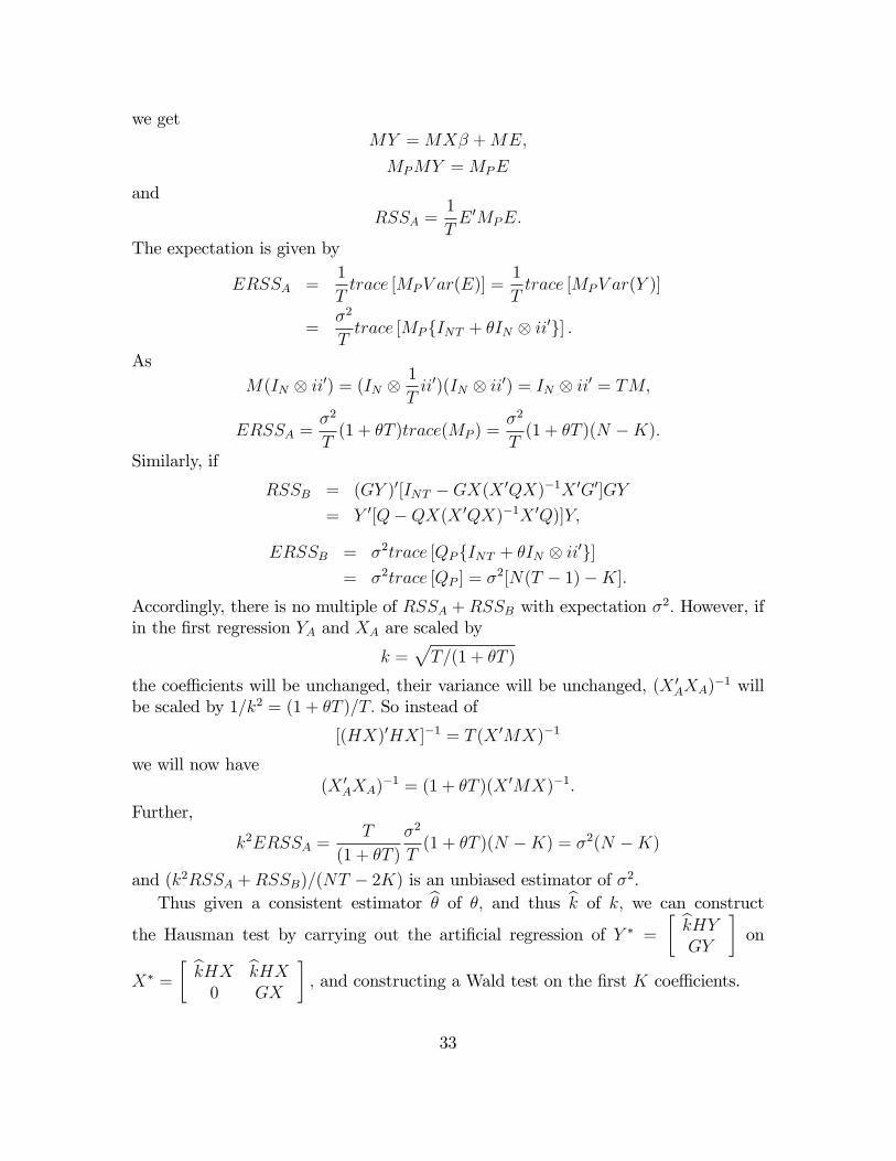
Ifk =
pT=(1 + T�)
then after using the residuals from the Between and Within regressions to calculatea consistent estimator b� of �; and thus bk of k; we can construct the Hausman test bycarrying out the arti�cial regression of Y � =
� bkHYGY
�on X� =
� bkHX bkHX0 GX
�;
and constructing a Wald test on the �rst K coe¢ cients. Such a test we refer to asan HR (Hausman Robust) test.In what follows, we will clarify to what extent an application of White�s formulae
for estimators of covariances matrices (White, 1984) in a panel data context providesa consistent estimator which is robust to heteroscedasticity and arbitrary correlationin the covariance matrix of the random disturbances. It may also control for thepresence of �xed e¤ects. This latter possibility may be accommodated if we makefurther assumptions, i.e. cross-sectional heteroscedasticity which takes on a �nitenumber of di¤erent values.Consider a simple panel data framework without �xed e¤ects
yi1 = �xi1 + "i1yi2 = �xi2 + "i2;...yiT = �xiT + "iT ; i = 1; :::; N;
where
E(�i�0
i) =
0B@ �2 : : : 0...
. . ....
0 : : : �2
1CA = �2IT = �:
Assume that in the complete model
(NT�NT )
= I � =
0BBB@� 0 : : : 0
0 �...
......
.... . . 0
0 : : : 0 �
1CCCA : (10)
7
De�ne
Xi =
0B@ xi1...xiT
1CA(T�1)
yi =
0B@ yi1...yiT
1CA(T�1)
�i =
0B@ "i1..."iT
1CA(T�1)
and rewrite the model as
yi(T�1)
= Xi�(T�1)
+ �i(T�1)
; i = 1; :::; N: (11)
This formulation allows us to consider panel data in the framework de�ned in White(1984). If we assume no cross-sectional correlation and N ! 1; all the hypothesesunderlying the derivation of White�s results are satis�ed. Hence, Proposition 7.2 inWhite (1984, p. 165) applies.
b� = N�1NXi=1
b�ib�i0 p�! � (12)
and b = I b� p�! :
However, while with uni-dimensional data sets we obtain heteroscedasticity consistentestimators because �i is a scalar, in the two dimensional case �i is a vector and weobtain a consistent estimator of the whole matrix �. Hence, by applying the result(12) in the panel data case we obtain a consistent estimator of the variance covariancematrix of the disturbances that also allows for the presence of dynamic e¤ects withingroups.Therefore, the estimators of the variance of the OLS estimators of � in the panel
data model (11) can be obtained by
\V ar(�) =
"NXi=1
�X
0
iXi
�#�1 NXi=1
X 0ibXi
"NXi=1
�X
0
iXi
�#�1: (13)
As stated by Arellano (1993), they are heteroscedasticity and autocorrelation con-sistent. Such estimators are the ones used in the implementation of the HR-test.This case is referred in White (1984) as contemporaneous covariance estimation.Woodridge (2002) also discusses robusti�cation of this and other Hausman tests inthe panel-data context.However, White (1984) also implements consistent estimators in another case that
explicitly takes into consideration a grouping structure of the data. Consider againthe panel data model (11). Replace assumption (10) by
8
(NT�NT )
=
0BBB@�1 0 : : : 0
0 �2...
......
.... . . 0
0 : : : 0 �N
1CCCA :In this context, in a slightly di¤erent notation from that used by White (1984, p.172-173), suitable for the panel data framework, we can obtain consistent estimators ofthe covariance matrix usingb = diag(b�1; b�2; : : : b�N)where b�i = T�1b�ib�i0:In other words, recall that White standard errors for OLS require the estimation
of (X0X)�1X 0X(X 0X)�1 without estimating the elements of the diagonal matrix individually. In the panel data model, is block diagonal, but for �xed T , asN ! 1, the corresponding estimator can be constructed. The resulting varianceestimator is not only robust to autocorrelation of arbitrary form within groups butit also allows for the possibility that individual error covariance matrices may di¤eracross groups. White�s second suggestion does not seem to have been implemented.
3 The Size of the Test
In this section we investigate the size distortion which occurs in the use of the standardHausman test when the basic assumptions (Lemma 2.1 in Hausman 1978) are notsatis�ed.Consider the panel data model (1) presented in Section 1. The Hausman test
investigates the presence of speci�cation errors of the form Cov(xit; �i) 6= 0: Therobust version proposed in Section 2 tests such orthogonality assumption betweenexplanatory variables and disturbances in presence of other forms of misspeci�cation.In particular we are interested in a possible misspeci�cation in the variance-covariancematrix of the disturbances arising, for instance, from the presence of measurementerrors in variables. This case may be the rule rather than the exception in appliedstudies.We want to test the hypothesis
Ho : Cov(xit; �i) = 0 (14)
against the alternativeH1 : Cov(xit; �i) 6= 0;
whenV ar("ijxit) 6= i: (15)
9
Hausman (1978) shows that under Ho the test statistic
h = bq0bV (bq)�1bq � �2K (16)
where, V (bq) is the asymptotic variance of q; and K is the length of q. The same teststatistic is obtained if we consider the vector bq equal to
bq1 = (b�WG � b�BN);or bq2 = (b�BG � b�BN);or bq3 = (b�WG � b�BG):
As Hausman and Taylor (1981) pointed out they are all nonsingular transforma-tions of one another. The estimate of the variance covariance matrix used in the threecases is
bV (bq1) = bV (b�WG)� bV (b�BN);or bV (bq2) = bV b�BG)� bV (b�BN);or bV (bq3) = bV (b�WG) + bV (b�BG):
If we are in presence of misspeci�cation of the form (15), none of the aboveexpressions gives a consistent estimate of the variance-covariance matrix, even underHo. The distribution of the test statistic under Ho need to be investigated. Thenominal size may be quite di¤erent from the observed one.To investigate the size distortion under normality, we use the distributions of
quadratic forms in normal random variables.2 In particular, we use the followingLemma.3
Lemma 1 (in Lemma 3.2 in Vuong, 1989). Let x � NK(0; V ); with rank (V ) �K; and let A be an K � K symmetric matrix. Then the random variable x0Ax isdistributed as a weighted sum of chi-squares with parameters (K; ); where is thevector of eigenvalues of AV:
This implies that x0Ax is �2r; where r = rank(A), if and only if AV is idempotent(Muirhead, 1982, Theorem 1.4.5).If A = V �1; i.e. in cases of no misspeci�cation, AV is idempotent. The theorem
is satis�ed and result (16) holds. The test statistic gives correct signi�cance levels.If A 6= V �1 but AV is idempotent then rank (A) < K and/or rank (V ) < K but
still (16) holds. We omit this case for simplicity of exposition.
2See, among others, Murihead (1982, Ch. 1), Johnson and Kotz (1970, Ch.29).3This Lemma holds also in the asymptotic case (using the Continuous Mapping Theorem, e.g.
White, 1984, Lemma 4.27).
10
If A 6= V �1 and AV is not idempotent, implying that the eigenvalues of AV arenot 0 or 1, the asymptotic distribution of the Hausman test under Ho is a weightedsum of central chi-squares
h �KXi=1
�iz2i
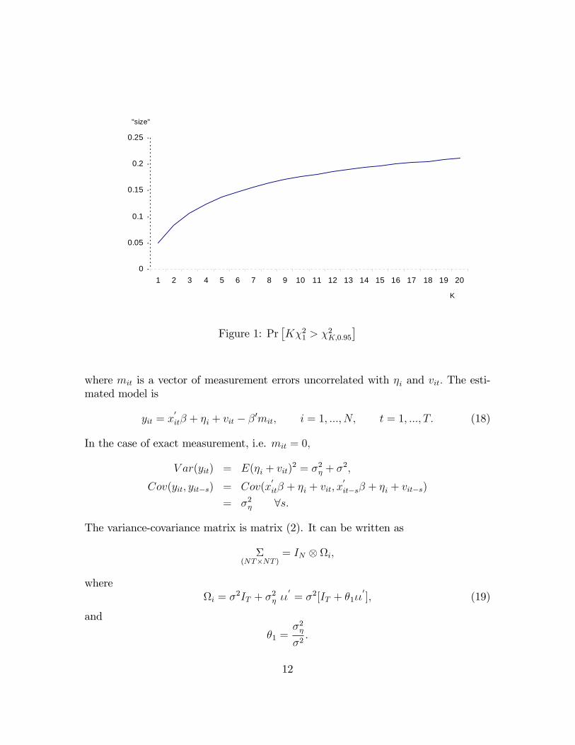
where z2i � �21 and �i are the eigenvalues of AV: This implies that the signi�cancelevels of the standard Hausman test are not correct.Consider �rst the limiting case where �1 ! K; �i ! 0; i = 2; ::; K: Figure 1
illustrates numerically that
Pr�K�21 > �
2K;�
�> �
where �2K;� is the critical value for a test of size � under the �2r distribution. In this
illustration � is set equal to 0.05.
In general we distinguish two e¤ects: a scale e¤ect ifKPi=1
�i 6= K, which is pre-
dictable (e.g. if �i = 2 8 i; h � 2�2K and a dispersion e¤ect if �i 6= �j; even ifKPi=1
�i = K: We normalize the weights and we conjecture that the dispersion e¤ect
is maximized in the tail of the distribution if we put all the weight on the largesteigenvalue, say the �rst one. Indeed, a thorough numerical investigation for K = 2,3 and 4 veri�es that this is the case, at least for these K values, when testing withsize less than 21.5%:Figure 1 shows Pr
�K�21 > �
2K;0:95
�, the probability that K� a �21 exceeds the 5%
critical value for a �2K . The graph shows that the size distortion is an increasingfunction of K: For instance, K = 2,3,4 gives worst-case sizes of 8.3%, 10.7%, and12.4%, while if K is equal to 14, the size is almost 4 time larger than the nominalsize. Appendix 2 provides details of the numerical investigation, and considers ananalytic approach.In certain simple contexts an expression for the eigenvalues of AV can be ana-
lytically derived. For instance, a common source of misspeci�cation in the variancecovariance matrix occurs when elements of the regressor matrix contain measurementerrors.Suppose the true model is
yit = z0
it� + �i + vit; i = 1; :::; N; t = 1; :::; T (17)
where z0it is a 1 �K vector of theoretical variables, �i � iid
�0; �2�
�; vit � iid (0; �2)
uncorrelated with the columns of zit and Cov (�i; vit) = 0: The observed variables are
xit = zit +mit;
11
0
0.05
0.1
0.15
0.2
0.25
1 2 3 4 5 6 7 8 9 10 11 12 13 14 15 16 17 18 19 20
K
"size"
Figure 1: Pr�K�21 > �
2K;0:95
�
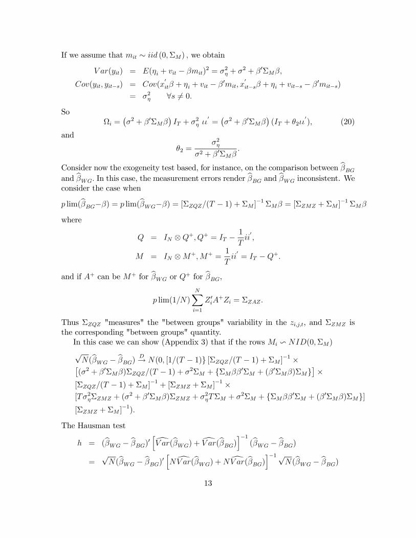
where mit is a vector of measurement errors uncorrelated with �i and vit: The esti-mated model is
yit = x0
it� + �i + vit � �0mit; i = 1; :::; N; t = 1; :::; T: (18)
In the case of exact measurement, i.e. mit = 0;
V ar(yit) = E(�i + vit)2 = �2� + �
2;
Cov(yit; yit�s) = Cov(x0
it� + �i + vit; x0
it�s� + �i + vit�s)
= �2� 8s:
The variance-covariance matrix is matrix (2). It can be written as
�(NT�NT )
= IN i;
wherei = �
2IT + �2� ��
0= �2[IT + �1��
0]; (19)
and
�1 =�2��2:
12
If we assume that mit � iid (0;�M) ; we obtain
V ar(yit) = E(�i + vit � �mit)2 = �2� + �
2 + �0�M�;
Cov(yit; yit�s) = Cov(x0
it� + �i + vit � �0mit; x0
it�s� + �i + vit�s � �0mit�s)
= �2� 8s 6= 0:
Soi =
��2 + �0�M�
�IT + �
2� ��
0=��2 + �0�M�
�(IT + �2��
0); (20)
and
�2 =�2�
�2 + �0�M�:
Consider now the exogeneity test based, for instance, on the comparison between b�BGand b�WG: In this case, the measurement errors render b�BG and b�WG inconsistent. Weconsider the case when
p lim(b�BG��) = p lim(b�WG��) = [�ZQZ=(T � 1) + �M ]�1�M� = [�ZMZ + �M ]
�1�M�
where
Q = IN Q+; Q+ = IT �1
Tii0;
M = IN M+;M+ =1
Tii0= IT �Q+:
and if A+ can be M+ for b�WG or Q+ for b�BG,
p lim(1=N)NXi=1
Z 0iA+Zi = �ZAZ :
Thus �ZQZ "measures" the "between groups" variability in the zi;j;t, and �ZMZ isthe corresponding "between groups" quantity.In this case we can show (Appendix 3) that if the rows Mi v NID(0;�M)pN(b�WG � b�BG) D! N(0; [1=(T � 1)g [�ZQZ=(T � 1) + �M ]�1 ��(�2 + �0�M�)�ZQZ=(T � 1) + �2�M + f�M��0�M + (�0�M�)�Mg
��
[�ZQZ=(T � 1) + �M ]�1 + [�ZMZ + �M ]�1 �
[T�2��ZMZ + (�2 + �0�M�)�ZMZ + �
2�T�M + �
2�M + f�M��0�M + (�0�M�)�Mg][�ZMZ + �M ]
�1):
The Hausman test
h = (b�WG � b�BG)0 hdV ar(b�WG) +dV ar(b�BG)i�1 (b�WG � b�BG)=
pN(b�WG � b�BG)0 hNdV ar(b�WG) +NdV ar(b�BG)i�1pN(b�WG � b�BG)
13
will have the same asymptotic distribution as
ha =pN(b�WG � b�BG)0p lim hNdV ar(b�WG) +NdV ar(b�BG)i�1pN(b�WG � b�BG)
and we also show in Appendix 3 that
NdV ar(b�WG)
p! f�2 + �0�M� � �0�M�
1
(T � 1)�ZQZ + �M��1
�M�g �
[�ZQZ + (T � 1)�M ]�1 :
Further
NdV ar(b�BG)p! fT�2� + �2 + �0�M� � �0�M [�ZMZ + �M ]
�1�M�g �[�ZMZ + �M ]
�1
Thus in terms of the notation of Lemma 3, for the asymptotic distribution
V = [1=(T � 1)g [�ZQZ=(T � 1) + �M ]�1 ��(�2 + �0�M�)�ZQZ=(T � 1) + �2�M + f�M��0�M + (�0�M�)�Mg
��
[�ZQZ=(T � 1) + �M ]�1 + [�ZMZ + �M ]�1 �
[T�2��ZMZ + (�2 + �0�M�)�ZMZ + �
2�T�M + �
2�M + f�M��0�M + (�0�M�)�Mg][�ZMZ + �M ]
�1):
and
A =
"f�2 + �0�M� � �0�M
h1
(T�1)�ZQZ + �M
i�1�M�g � [�ZQZ + (T � 1)�M ]�1
+fT�2� + �2 + �0�M� � �0�M [�ZMZ + �M ]�1�M�g � [�ZMZ + �M ]
�1
#�1
Note that when � = 0; then AV = I:
V = [1=(T � 1)] [�ZQZ=(T � 1) + �M ]�1 ���2�ZQZ=(T � 1) + �2�M
�� [�ZQZ=(T � 1) + �M ]�1
+ [�ZMZ + �M ]�1 � [T�2��ZMZ + �
2�ZMZ + �2�T�M + �
2�M ] [�ZMZ + �M ]�1
= [1=(T � 1)]�2 [�ZQZ=(T � 1) + �M ]�1
+ [�ZMZ + �M ]�1 (T�2� + �
2)[�ZMZ + �M ] [�ZMZ + �M ]�1
= [1=(T � 1)]�2 [�ZQZ=(T � 1) + �M ]�1
+(T�2� + �2) [�ZMZ + �M ]
�1
14
A =��2 [�ZQZ + (T � 1)�M ]�1 + fT�2� + �2g � [�ZMZ + �M ]
�1��1so AV = I:When �M = 0; we obtain the usual results for the standard case withoutmeasurement error,
V = �2[1=(T � 1)g [�ZQZ=(T � 1)]�1 + [T�2� + �2] [�ZMZ ]�1
A =��2��1ZQZ + fT�2� + �2g��1ZMZ
��1:
Now let �Q = �ZQZ=(T � 1); ��2 = �2 + �0�M�; c =�M�; ���2 = ��2 + T�2�;so
V = [1=(T � 1)] [�Q + �M ]�1���2[�Q + �M ] + cc
0� [�Q + �M ]�1 +[�ZMZ + �M ]
�1 ����2[�ZMZ + �M ] + cc0� [�ZMZ + �M ]
�1
= [1=(T � 1)]���2[�Q + �M ]
�1 + dd0�+����2[�ZMZ + �M ]
�1 + ee0�
where d = [�Q + �M ]�1 c; and e = [�ZMZ +�M]
�1c: These are just the inconsisten-cies, which we are assuming equal.
A =
�1=(T � 1)f��2 � c0 [�Q + �M ]�1 cg � [�Q + �M ]�1+f���2 � c0 [�ZMZ + �M ]
�1 cg � [�ZMZ + �M ]�1
��1The simplest case to examine is when �Q = �ZMZ , p lim b�WG = p lim
b�BG for all�; let �QM = �Q + �M = �ZMZ + �M : Noting d = e; we have
V = �+2�QM�1 + 2dd0
where
�+2 = [1=(T � 1)]��2 + ���2
= [T=(T � 1)]��2 + T�2�
A = [�++2��1QM ]�1
where
�++2 = [1=(T � 1)]f��2 � c0��1QMcg+ ���2 � c0��1QMc;= [T=(T � 1)][��2 � c0��1QMc] + T�2�
and AV has the same eigenvalues as
A1=2V A1=2 =�+2
�++2I +
2
�++2�QM
1=2dd0�QM1=2
and has K � 1 eigenvalues ofk = �+2=�++2
15
and one of
k + (2=�++2)d0�QMd = k+(2=�++2)c0��1QMc
= k+(2=�++2)�0�M��1QM�M�:
Thus the size distortion depends on scalar quantities,
k =�+2
�++2=
1
1� k� ;
k� =�+2 � �++2
�+2=
�0�M��1QM�M�
[T=(T � 1)]f�2 + �0�M�g+ T�2�
and the larger root is
�+2
�++2+
2
�++2k��+2 =
1
1� k� [1 + 2k�] :
�0�M��1QM�M� = �0�
1=2M [�
1=2M (�Q + �M)
�1�1=2M ]�
1=2M �
= �0�1=2M [�
�1=2M �Q�
�1=2M +I]�1�
1=2M �
If we now write = �
1=2M �
is the vector of parameters in the model
yi = [Zi +Mi] ��1=2M �
1=2M � + �ii+ "i
= Z�i +M�i + �ii+ "i
where the rows ofMi are NID(0; I) and Z�i = Zi��1=2M ) Zi = Z
�i �
1=2M ) Z 0iM
+Zi =
�1=2M Z�0i M
+Z�i �1=2M
k� = 0[��1=2M �ZMZ�
�1=2M +I]�1 =�+2
= 0 [�Z�MZ� + I]�1 =
�[T=(T � 1)]f�2 + 0 g+ T�2�
�(21)
The components of the variance of yi;t are
V ar(yi;t) = 0 + �2� + �
2
so an interpretation of our result is that if one takes one component of the variance, 0 ; downweights it by the between sums of squares of the unobserved �true�variables(in the model with standardised measurement errors), to produce 0 [�Z�MZ� + I]
�1 ;then the �size�distortion depends on k�, as in (21), and the asymptotic distributionof the Hausman test is not �2(K); but a weighted sum of K �2(1); K � 1 weights
16
being 1=(1 � k�); with one of [1 + 3k�=(1� k�)] : It also follows that a lower boundto the distortion is provided by multiplying a �2(K) by 1=(1� k�):A number of quali�cations are in order. This only occurs if the inconsistency of
within and between estimators is equal, and, further, the within group sum of squaresmatrix, and between group sum of squares matrix, are equal:
�ZMZ ;= limN!1
1
N
NXi=1
ZiM+Zi;= �Q;=
1
T � 1 limN!1
1
N
NXi=1
ZiQ+Zi:
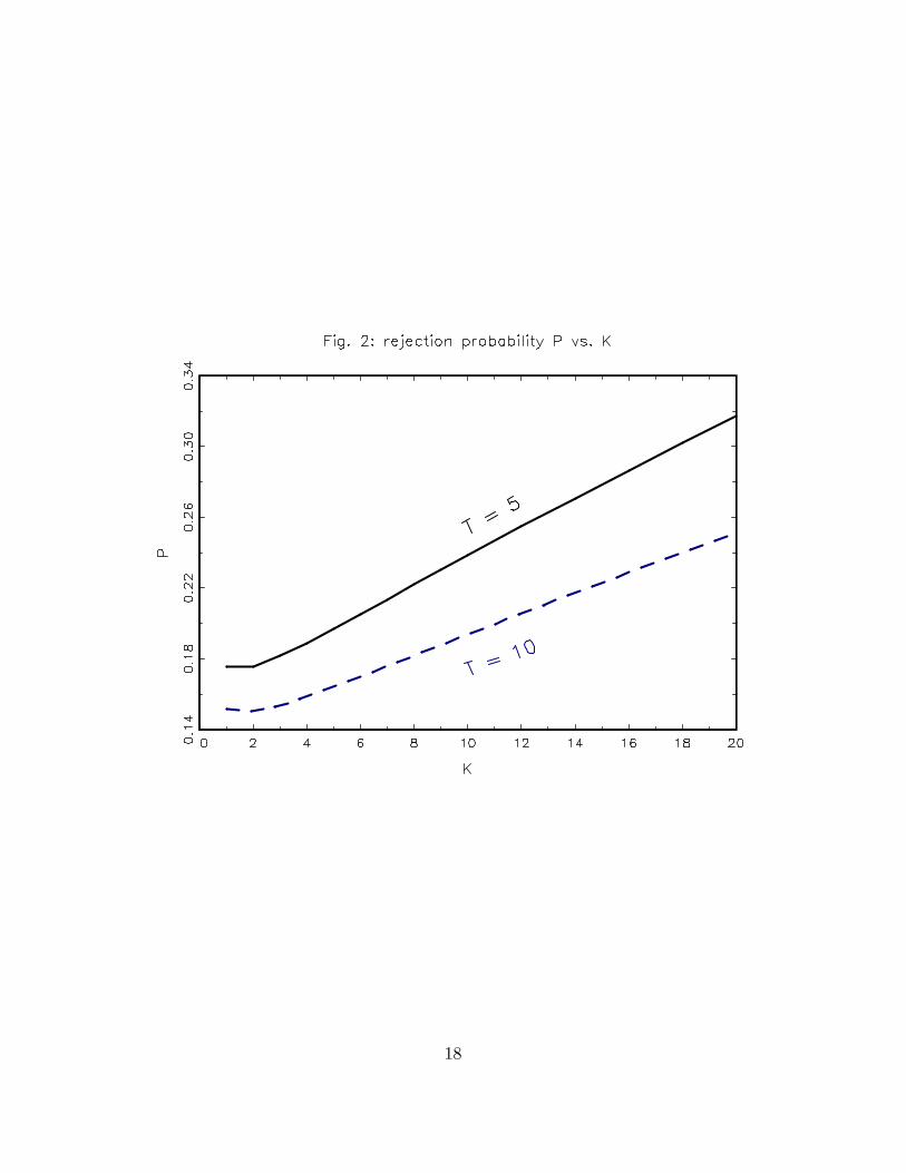
The equality of p lim(b�BG � �) and p lim(b�WG � �) is required to ensure that theasymptotic �size�is not 1. (Thus the Hausman test can be regarded as a (consistent)test of equality of these �inconsistencies�).The equality of �ZMZ and �Q simpli�esthe result and is an aid to interpretability. We also assume that the rows of Mi,the measurement errors, are NID(0;�M): Some assumption about fourth momentsis required, and this appears the simplest.We can plot the size distortion for assumed values of T;K; 0 ; 0 [�Z�MZ� + I]
�1 ; �2�and �2: If T = 5 or 10; 1 � K � 20; 0 = 1; �2� = �2 = 0:1; and 0 [�Z�MZ� + I]
�1 =0:5; we have Figure 2.We can relax the assumption that �Q = �ZMZ by observing that V is of the form
V = k1B + k2C + d�d�0
and A is of the formA = (k3B + k4C)
�1
where
B = [�Q + �M ]�1; C = [�ZMZ + �M ]
�1
k1 = [1=(T � 1)]��2; k2 = ���2
d� = f1 + 1=(T � 1)g1=2d = fT=(T � 1)g1=2d;k3 = 1=(T � 1)f��2 � c0B�1cg; <k1k4 = f���2 � c0C�1cg; < k2
and B and C are positive de�nite. We see that A is �too small�, and the test will beoversized.
V = B1=2[k1I + k2B�1=2CB�1=2 +B�1=2d�d�0B�1=2]B1=2
A�1 = B1=2[k3I + k4B�1=2CB�1=2]B1=2
LetD = B�1=2CB�1=2 = P�P 0
17
18
where P is orthogonal, � diagonal, with as diagonal elements �i the eigenvalues ofD. Then
V = B1=2P [k1I + k2� + P0B�1=2d�d�0B�1=2P ]P 0B1=2
A =�B1=2P [k3I + k4�]P
0B1=2��1
= B�1=2P [k3I + k4�]�1P 0B�1=2
and thus
AV = B�1=2P [k3I + k4�]�1[k1I + k2� + P
0B�1=2d�d�0B�1=2P ]P 0B1=2
= B�1=2P [diag([k3 + k4�i]�1)fdiag(k1 + k2�i)
+P 0B�1=2d�d�0B�1=2Pg]P 0B1=2
which has the same eigenvalues as
fdiag(k1 + k2�ik3 + k4�i
)
+diag([k3 + k4�i]�1fP 0B�1=2d�d�0B�1=2Pg
The second matrix has rank 1, and the eigenvalues of the whole matrix are boundedbetween the smallest of k0;i = (k1 + k2�i)=(k3 + k4�i) and the largest of k0;i +d�0B�1d�=(k3 + k4�i): �i are the eigenvalues of D = B�1=2CB�1=2; or of B�1C =[�Q + �M ][�ZMZ + �M ]
�1: d = [�Q + �M ]�1 c = [�ZMZ +�M]
�1c =Bc =Cc
d�0B�1d� = fT=(T � 1)gc0Bc = fT=(T � 1)g�0�M [�ZMZ + �M ]�1�M�
= fT=(T � 1)g 0 [�Z�MZ� + I]�1
k1 = [1=(T � 1)]��2; ��2 = �2 + �0�M� = �2 + 0 k2 = ���2 = ��2 + T�2�
k3 = 1=(T � 1)f��2 � c0B�1cg =1=(T � 1)��2 + 0 � 0 [�Z�MZ� + I]
�1 �<k1
k4 = f���2 � c0C�1cg = �2 + 0 + T�2� � 0 [�Z�MZ� + I]�1 < k2
Thus
�+2 = [1=(T � 1)]��2 + ���2 = k1 + k2�++2 = [1=(T � 1)]f��2 � c0��1QMcg+ ���2 � c0��1QMc =k3 + k4
k0;i =k1 + k2�ik3 + k4�i
=k1 + k2 + k2(�i � 1)k3 + k4 + k4(�i � 1)
=�+2[1 + k2(�i � 1)=�+2]�++2[1 + k4(�i � 1)=�++2]
= k[1 + k2(�i � 1)=�+2][1 + k4(�i � 1)=�++2]
19
Thus comparing this case with the B = C case, we are introducing more variabilityinto the eigenvalues, which as we have seen , may well increase the �size�of the test.(Thus the �size�is sensitive to the relative magnitude of the intra-group and inter-group variations of the covariates, �ZQZ and �ZMZ). Our conclusion is somewhatdispiriting: a signi�cant Hausman statistic may arise from measurement error, as itis implicitly comparing the inconsistencies: but cannot be used to test if the inconsis-tencies are equal, as the �size�may considerably exceed its nominal value, even whenthe inconsistencies are equal.
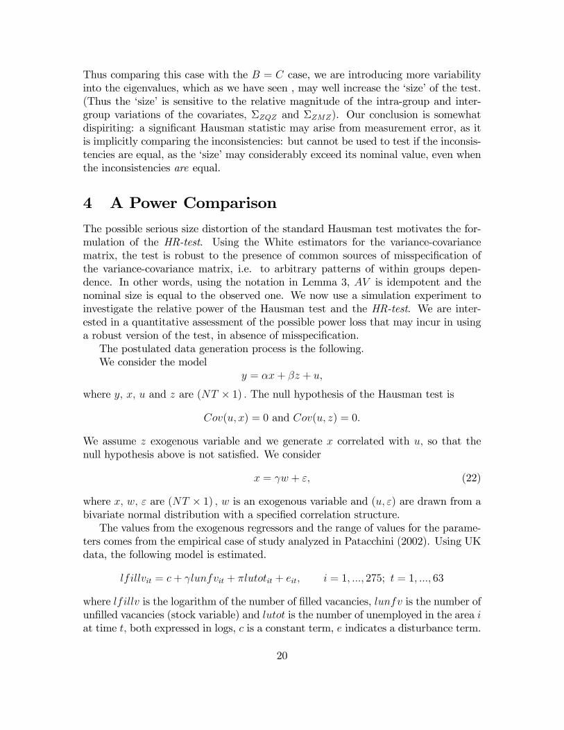
4 A Power Comparison
The possible serious size distortion of the standard Hausman test motivates the for-mulation of the HR-test. Using the White estimators for the variance-covariancematrix, the test is robust to the presence of common sources of misspeci�cation ofthe variance-covariance matrix, i.e. to arbitrary patterns of within groups depen-dence. In other words, using the notation in Lemma 3, AV is idempotent and thenominal size is equal to the observed one. We now use a simulation experiment toinvestigate the relative power of the Hausman test and the HR-test. We are inter-ested in a quantitative assessment of the possible power loss that may incur in usinga robust version of the test, in absence of misspeci�cation.The postulated data generation process is the following.We consider the model
y = �x+ �z + u;
where y; x; u and z are (NT � 1) : The null hypothesis of the Hausman test is
Cov(u; x) = 0 and Cov(u; z) = 0:
We assume z exogenous variable and we generate x correlated with u; so that thenull hypothesis above is not satis�ed. We consider
x = w + "; (22)
where x; w; " are (NT � 1) ; w is an exogenous variable and (u; ") are drawn from abivariate normal distribution with a speci�ed correlation structure.The values from the exogenous regressors and the range of values for the parame-
ters comes from the empirical case of study analyzed in Patacchini (2002). Using UKdata, the following model is estimated.
lfillvit = c+ lunfvit + �lutotit + eit; i = 1; :::; 275; t = 1; :::; 63
where lfillv is the logarithm of the number of �lled vacancies, lunfv is the number ofun�lled vacancies (stock variable) and lutot is the number of unemployed in the area iat time t; both expressed in logs, c is a constant term, e indicates a disturbance term.
20
The estimates of and �; 0:5 and 0:4, have been used in the simulation experimentfor � and � respectively. Also, the best prediction for un�lled vacancies (lunfv) isfound to be
lunfvit = 1:2 ln otvit; i = 1; :::; 275; t = 1; :::; 63;
where lnotv is the logarithm of the number of monthly noti�ed vacancies (�ow vari-able). In our experiment design, the real values for lutot and lnotv have been used asexogenous variables, i.e. respectively z and w: The endogenous variable lunfv, i.e.x, has been constructed according to the structure (22)
x = 1:2w + ":
The equation estimated isy = 0:5x+ 0:4z + u;
where (u; ") are constructed as draws from a multivariate normal distribution withthe speci�ed correlation coe¢ cient rho of (0; 0:05; 0:10; : : : ; 0:95):Six sample sizes, typically encountered in applied panel data studies are used.
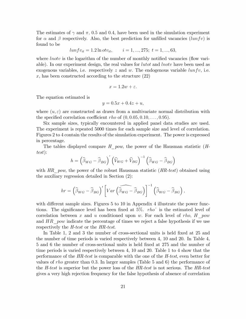
The experiment is repeated 5000 times for each sample size and level of correlation.Figures 2 to 4 contain the results of the simulation experiment. The power is expressedin percentage.The tables displayed compare H_pow, the power of the Hausman statistic (H-
test):
h =�b�WG � b�BG�0 �bVWG + bVBG��1 �b�WG � b�BG�
with HR_pow, the power of the robust Hausman statistic (HR-test) obtained usingthe auxiliary regression detailed in Section (2):
hr =�b�WG � b�BG�0 � \
V ar�b�WG � b�BG���1 �b�WG � b�BG� ;
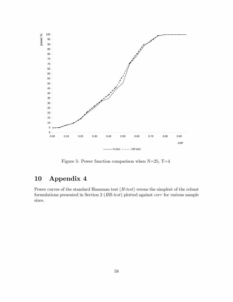
with di¤erent sample sizes. Figures 5 to 10 in Appendix 4 illustrate the power func-tions. The signi�cance level has been �xed at 5%. rho^ is the estimated level ofcorrelation between x and u conditioned upon w: For each level of rho; H_powand HR_pow indicate the percentage of times we reject a false hypothesis if we userespectively the H-test or the HR-test.In Table 1, 2 and 3 the number of cross-sectional units is held �xed at 25 and
the number of time periods is varied respectively between 4, 10 and 20. In Table 4,5 and 6 the number of cross-sectional units is held �xed at 275 and the number oftime periods is varied respectively between 4, 10 and 20. Table 1 to 4 show that theperformance of the HR-test is comparable with the one of the H-test, even better forvalues of rho greater than 0:3: In larger samples (Table 5 and 6) the performance ofthe H-test is superior but the power loss of the HR-test is not serious. The HR-testgives a very high rejection frequency for the false hypothesis of absence of correlation
21
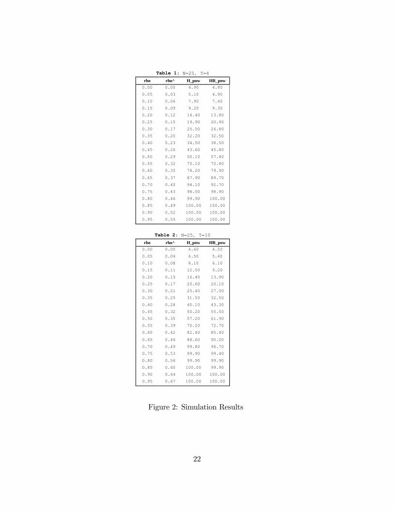
Table 1: N=25, T=4
rho rho^ H_pow HR_pow0.00 0.00 4.90 4.80
0.05 0.03 5.10 4.90
0.10 0.06 7.90 7.40
0.15 0.09 9.20 9.30
0.20 0.12 14.40 13.80
0.25 0.15 19.90 20.90
0.30 0.17 25.50 26.80
0.35 0.20 32.20 32.50
0.40 0.23 34.50 38.50
0.45 0.26 43.60 45.80
0.50 0.29 50.10 57.40
0.55 0.32 70.10 70.80
0.60 0.35 78.20 79.90
0.65 0.37 87.90 89.70
0.70 0.40 94.10 92.70
0.75 0.43 98.50 98.90
0.80 0.46 99.90 100.00
0.85 0.49 100.00 100.00
0.90 0.52 100.00 100.00
0.95 0.55 100.00 100.00
Table 2: N=25, T=10
rho rho^ H_pow HR_pow0.00 0.00 4.60 4.50
0.05 0.04 6.50 5.40
0.10 0.08 8.10 6.10
0.15 0.11 12.50 9.20
0.20 0.15 16.40 13.90
0.25 0.17 20.60 20.10
0.30 0.21 25.40 27.50
0.35 0.25 31.50 32.50
0.40 0.28 40.10 43.30
0.45 0.32 50.20 55.50
0.50 0.35 57.20 61.90
0.55 0.39 70.20 72.70
0.60 0.42 82.40 85.40
0.65 0.46 88.60 90.00
0.70 0.49 99.80 96.70
0.75 0.53 99.90 99.40
0.80 0.56 99.90 99.90
0.85 0.60 100.00 99.90
0.90 0.64 100.00 100.00
0.95 0.67 100.00 100.00
Figure 2: Simulation Results
22
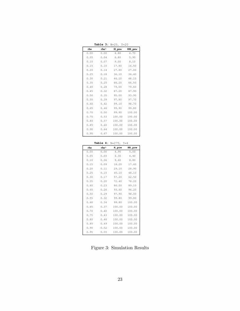
Table 3: N=25, T=20
rho rho^ H_pow HR_pow0.00 0.00 4.80 4.70
0.05 0.04 6.80 5.90
0.10 0.07 9.00 8.10
0.15 0.10 17.80 16.50
0.20 0.14 27.80 27.00
0.25 0.18 36.10 36.40
0.30 0.21 46.20 48.10
0.35 0.25 66.20 66.50
0.40 0.28 79.00 79.60
0.45 0.32 87.20 87.90
0.50 0.35 95.00 93.90
0.55 0.39 97.80 97.70
0.60 0.42 99.10 98.70
0.65 0.46 99.90 99.80
0.70 0.50 99.90 100.00
0.75 0.53 100.00 100.00
0.80 0.57 100.00 100.00
0.85 0.60 100.00 100.00
0.90 0.64 100.00 100.00
0.95 0.67 100.00 100.00
Table 4: N=275, T=4
rho rho^ H_pow HR_pow
0.00 0.00 4.90 5.00
0.05 0.03 6.30 6.40
0.10 0.06 9.60 8.80
0.15 0.09 18.20 17.60
0.20 0.11 29.10 28.90
0.25 0.15 45.10 48.10
0.30 0.17 57.20 62.50
0.35 0.20 72.40 78.20
0.40 0.23 86.00 89.10
0.45 0.26 93.60 96.20
0.50 0.29 97.90 98.00
0.55 0.32 99.80 99.80
0.60 0.34 99.80 100.00
0.65 0.37 100.00 100.00
0.70 0.40 100.00 100.00
0.75 0.43 100.00 100.00
0.80 0.46 100.00 100.00
0.85 0.49 100.00 100.00
0.90 0.52 100.00 100.00
0.95 0.55 100.00 100.00
Figure 3: Simulation Results
23

Table 5: N=275, T=10
rho rho^ H_pow HR_pow
0.00 0.00 5.00 4.90
0.05 0.03 9.80 6.40
0.10 0.06 26.10 15.10
0.15 0.09 61.00 34.00
0.20 0.12 87.80 55.10
0.25 0.15 97.80 74.10
0.30 0.18 98.90 86.50
0.35 0.20 99.80 93.40
0.40 0.23 99.90 97.90
0.45 0.26 100.00 98.90
0.50 0.29 100.00 99.90
0.55 0.32 100.00 100.00
0.60 0.35 100.00 100.00
0.65 0.38 100.00 100.00
0.70 0.41 100.00 100.00
0.75 0.44 100.00 100.00
0.80 0.47 100.00 100.00
0.85 0.50 100.00 100.00
0.90 0.53 100.00 100.00
0.95 0.55 100.00 100.00
Table 6: N=275, T=20
rho rho^ H_pow HR_pow
0.00 0.00 5.10 4.70
0.05 0.03 18.40 6.40
0.10 0.06 59.70 18.90
0.15 0.09 91.10 40.10
0.20 0.12 99.80 62.40
0.25 0.15 99.90 75.50
0.30 0.18 99.90 87.40
0.35 0.20 100.00 94.10
0.40 0.23 100.00 98.90
0.45 0.26 100.00 100.00
0.50 0.29 100.00 100.00
0.55 0.32 100.00 100.00
0.60 0.35 100.00 100.00
0.65 0.38 100.00 100.00
0.70 0.41 100.00 100.00
0.75 0.44 100.00 100.00
0.80 0.47 100.00 100.00
0.85 0.50 100.00 100.00
0.90 0.53 100.00 100.00
0.95 0.56 100.00 100.00
Figure 4: Simulation Results
24
between x and u; starting from levels of correlation around 0:3 (86:5% and 87:4%respectively in Table 5 and 6) and it detects the endogeneity problem almost surelyas soon as rho is higher than 0:4 (97:9% and 98:9% respectively in Table 5 and 6).Taking the results as a whole, the simulation experiment provides evidence that theperformance of the HR-test in terms of power is satisfying in large samples and evenbetter than the one given by the H-test in small samples.In addition, it is worthwhile noting that a version of the Hausman test imple-
mented in most econometric software, which is generally used in empirical studies, isthe one based on the comparison between b�WG and b�BN , i.e.
h =�b�WG � b�BN�0 �bVWG � bVBN��1 �b�WG � b�BN� :
The problem related with this approach is that, in �nite samples, the di¤erencebetween the two estimated variance-covariance matrices of the parameters estimates(i.e. bVWG � bVBG) may not be positive de�nite. In this cases, the use of a codeimplementing a di¤erent Hausman statistic or the formulation of the Hausman testusing an auxiliary regressions (e.g. the one proposed by Davidson and McKinnon(1993, p. 236), which is now already implemented in some statistical packages, or the(robust) one presented in this paper) are needed to obtain a test outcome.
5 Conclusions
Our recommendation is to use the Hausman test framework for the comparison ofappropriate panel data estimators and to construct a version of the test robust todeviations from the classical errors assumption, as proposed in this paper. This test,the HR-test, gives correct signi�cance levels in common cases of misspeci�cation of thevariance-covariance matrix and has a power comparable to the Hausman test whenno evidence of misspeci�cation is present. The power of the HR-test can be evenhigher in small samples. It can be easily implemented using a standard econometricpackage.The relationship between the eigenvalues corresponding to the quadratic form
that is the Hausman test statistic, and the size of the test, needs to be established ingenerality. A proof is under construction.
25
6 References
References
[1] Arellano, M. (1993). On the Testing of Correlated E¤ects with Panel Data,Journal of Econometrics, 59, 87-97.
[2] Ahn, S.C. and Low, S. (1996). A Reformulation of the Hausman Test for Regres-sion Models with Pooled Cross Sectional Time Series Data, Journal of Econo-metrics, 71, 309-319.
[3] Balestra, P. and Nerlove, M. (1966). Pooling Cross Section and Time Series Data,Econometrica, 34, 585-612.
[4] Baltagi, B.H. (1996). Testing for Random Individual and Time E¤ects using aGauss-Newton Regression, Economics Letters, 50, 189-192.
[5] Baltagi, B.H. (1997). Problems and Solutions, Econometric Theory, 13, 757.
[6] Baltagi, B.H. (1998). Problems and Solutions, Econometric Theory, 14, 527.
[7] Davidson, R. and MacKinnon, J.G. (1993). Estimation and Inference in Econo-metrics, Oxford University Press.
[8] Durbin, J. (1954). Errors in Variables. Review of the International StatisticalInstitute, 22, 23-32.
[9] Golub, G.H. and Van Loan, C.F. (1983). Matrix Computations, third edition,North Oxford Academic Press.
[10] Griliches, Z. and Hausman, J.A. (1986). Error in Variables in Panel Data, Journalof Econometrics, 31, 93-118.
[11] Hansen, L. (1982). Large Sample Properties of Generalized Method of MomentEstimators, Econometrica, 50, 517-533.
[12] Hausman, J.A. (1978). Speci�cation Tests in Econometrics, Econometrica, 46,1251-1271.
[13] Hausman, J.A. and Taylor, W.E. (1981). Panel Data and Unobservable Individ-ual E¤ects, Econometrica, 49, 1377-1398.
[14] Holly, A. (1982). A Remark on Hausman�s Speci�cation Test, Econometrica, 50,749-760.
[15] Johnson, N.L. and Kotz, S. (1970). Continuous Univariate Distributions, NewYork: John Wiley and Sons.
26

[16] Kakwani, N.C. (1967). The Unbiasedness of Zellner�s Seemingly Unrelated Re-gression Equation Estimators, Journal of the American Statistical Association,82, 141-2
[17] Maddala, G.S. (1971). The Use of Variance Components Models in Pooling CrossSection and Time Series Data, Econometrica, 39, 341-358.
[18] Magnus, J.R. and H. Neudecker, (1988)Matrix Di¤erential Calculus John Wileyand Sons.
[19] Muirhead, R.J. (1982). Aspects of Multivariate Statistical Theory, New York:John Wiley and Sons.
[20] Newey, W. K. and D. McFadden (1994), "Large Sample Estimation and Hypoth-esis Testing," in Handbook of Econometrics, vol. iv, ed. by R. F. Engle and D.L. McFadden, pp. 2111-2245, Amsterdam: Elsevier.
[21] Nerlove, M. (1971). A Note on Error Components Models, Econometrica, 39,383-396.
[22] O�Brien, R.J. and Patacchini, E. (2003) Testing the Exogeneity Assumption inPanel Data Models with "Non-Classical" Disturbances, Discussion Papers inEconomics and Econometrics 0302, University of Southampton
[23] Patacchini, E. (2002). Unobservable Factors and Panel Data Sets: the Case ofMatched Employee-Employer Data, Discussion Papers in Economics and Econo-metrics 0202, University of Southampton.
[24] Ruud, P. (2000) An Introduction to Classical Econometric Theory. Oxford: Ox-ford University Press
[25] Vuong, Q. (1989). Likelihood Ratio Tests for Model Selection and Non-NestedHypotheses, Econometrica, 57, 307-333.
[26] Sheil, J. and O�Muircheartaigh, I. (1977) Algorithm AS106: The Distributionof Non-Negative Quadratic Forms in Normal Variables, Applied Statistics, 26,92-98
[27] White, H. (1984). Asymptotic Theory for Econometricians, Academic Press, NewYork.
[28] Wooldridge, J.M. (1995), second edition (2002) Econometric Analysis of CrossSection and Panel Data. Cambridge, Mass: MIT Press
[29] Wu, D. (1973). Alternatives Tests of Independence between Stochastic Regressorsand Disturbances. Econometrica, 41, 733-750.
27
7 Appendix 1
Lemma 2 If
b� = (X 0X)�1X 0y; b�� = (X�0X�)�1X�0y;
X� = XA; jAj 6= 0;b" = y �Xb�;b"� = y �X�b��;then
(X�0X�)�1 = A�1(X 0X)�1A0�1b�� = A�1b�b"� = b"Proof.
(X�0X�)�1 = (A0X 0XA)�1 = A�1(X 0X)�1A0�1:b�� = (X�0X�)�1X�0y = A�1(X 0X)�1A0�1A0X 0y = A�1b�:b"� = y �X�b�� = y �XAA�1b� = y �Xb� = b"Lemma 3 If b�A = (X 0
AXA)�1X 0
AyA;b�B = (X 0
BXB)�1X 0
ByB;b"A = yA �XAb�A;b"B = yB �XB
b�BX� =
�XA XA
0 XB
�; y� =
�yAyB
�; b�� = (X�0X�)�1X�0y
b"� = y� �X�b��then b�� = " b�A � b�Bb�B
#;b"� = � b"Ab"B
�Proof. Let
X =
�XA 00 XB
�;) X� = X
�I I0 I
�= XA say
A�1 =
�I �I0 I
�Further, it is an exercise in elementary matrix algebra to show that
b� = (X 0X)�1X 0y =
" b�Ab�B#;b" = y �Xb� = � b"Ab"B
�:
28
So applying Lemma 2,
b�� = A�1b� = � I �I0 I
�" b�Ab�B#=
" b�A � b�Bb�B#
and b"� = b" = � b"Ab"B�
Return now to model (9). Results (??) and (??) in Lemma ?? directly followfrom the application of Lemma 2 and 3. Next, we will prove the remaining result inLemma ??, i.e. equality (??).Let
H+ =1
Ti0; H = IN H+; H 0H =
1
TMb�bg = [(HX)0(HX)]�1(HX)0(HY ) = (X 0MX)�1X 0MYb�wg = [(QX)0(QX)]�1(QX)0(QY ) = (X 0QX)�1X 0QY
Further, let G+ be Arellano and Bover�s (1990) forward orthogonal deviations matrix,(T � 1)� T; such that
G+i = 0; G+G+0= I(T�1); G
+0G+ = Q+ = IT �1
Tii0
G = IN G+; G0G = Q;GG0 = IN I(T�1) = IN(T�1)b�wg = [(GX)0(GX)]�1(GX)0(GY ) = (X 0QX)�1X 0QY
and identifying HX and HY with XA and YA; GX and GY with XB and YB; we
see that the arti�cial regression of Y � =�HYGY
�on X� =
�HX HX0 GX
�gives
coe¢ cients b�� = " b�bg � b�wgb�wg#: In this case,
V ar(Y �) =
�HV ar(Y )H 0 0
0 GV ar(Y )G0
�:
If � = �2�=�2we have
GV ar(Y )G0 = �2G(INT + �IN ii0)G0
= �2GG0 as G+i = 0
= �2IN(T�1)
29
and
HV ar(Y )H 0 = �2H(INT + �IN ii0)H 0
= �2[IN H+](INT + �IN ii0)[IN H+0]
= �2[IN (H+H+0) + �IN (H+ii0H+0):
AsH+ =
1
Ti0; H+i = 1; H+H+0 =
1
T;
HV ar(Y )H 0 = �2[1
TIN + �IN ] =
�2
T(1 + T�)IN :
Assembling our results,
V ar(Y �) =
��2
T(1 + T�)IN 0
0 �2IN(T�1)
�:
If now eX =
�HX 00 GX
�;
V ar(b��) = (X�0X�)�1X�0V ar(Y �)X�(X�0X�)�1
= A�1( eX 0 eX)�1 eX 0V ar(Y �) eX( eX 0 eX)�1A�10 :Next, we calculate this variance by separating the di¤erent components.eX 0V ar(Y �) eX =
�X 0H 0 00 X 0G0
� ��2
T(1 + T�)IN 0
0 �2IN(T�1)
� �HX 00 GX
�= �2
�X 0H 0 00 XG0
� �(� + 1=T )HX 0
0 GX
�= �2
�(�=T + 1=T 2)X 0MX 0
0 X 0QX
�.
( eX 0 eX)�1 = � T (X 0MX)�1 00 (X 0QX)�1
�:
Thus( eX 0 eX)�1 eX 0V ar(Y �) eX 0( eX 0 eX)�1= �2
�T (X 0MX)�1 0
0 (X 0QX)�1
���
(�=T + 1=T 2)X 0MX 00 X 0QX
� �T (X 0MX)�1 0
0 (X 0QX)�1
�= �2
�(T� + 1)(X 0MX)�1 0
0 (X 0QX)�1
�
30
and
A�1( eX 0 eX)�1 eX 0V ar(Y �) eX 0( eX 0 eX)�1A�10= �2
�I �I0 I
� �(T� + 1)(X 0MX)�1 0
0 (X 0QX)�1
� �I 0�I I
�= �2
�(T� + 1)(X 0MX)�1 �(X 0QX)�1
0 (X 0QX)�1
� �I 0�I I
�= �2
�(T� + 1)(X 0MX)�1 + (X 0QX)�1 �(X 0QX)�1
�(X 0QX)�1 (X 0QX)�1
�: (23)
We now need to �nd the variance-covariance matrix the arti�cial regression willassume. This will be proportional to
(X�0X�)�1 = (A0 eX 0 eXA)�1 = A�1( eX 0 eX)�1A�10=
�I �I0 I
� �T (X 0MX)�1 0
0 (X 0QX)�1
� �I 0�I I
�=
�T (X 0MX)�1 � (X 0QX)�1
0 (X 0QX)�1
� �I 0�I I
�=
�T (X 0MX)�1 + (X 0QX)�1 � (X 0QX)�1
� (X 0QX)�1 (X 0QX)�1
�: (24)
By comparing (23) with (24) it appears that an arti�cial regression is a valuable deviceto estimate a suitable variance-covariance matrix. This variance is estimated using a(White) robust OLS estimator which uses a consistent estimator of X�0V ar(Y �)X�
under the assumption that V ar(Y �) is diagonal. Next, we derive this consistentestimator. Following the steps used in the derivation of V ar(b��) above, we separatethe di¤erent components.
eX 0V ar(Y �) eX=
�X 0H 0 00 X 0G0
� ��2 00 �2
� �HX 00 GX
�= �2
�X 0H 0 00 X 0G0
� � 00
� �HX 00 GX
�= �2
�X 0H 0 00 X 0G0
� �HX 00 GX
�= �2
�XH 0HX 0
0 X 0G0GX
�:
( eX 0 eX)�1 = � T (X 0MX)�1 00 (X 0QX)�1
�:
31

Thus
( eX 0 eX)�1 eX 0V ar(Y �) eX 0( eX 0 eX)�1= �2
�T (X 0MX)�1 0
0 (X 0QX)�1
���
XH 0HX 00 X 0G0GX
� �T (X 0MX)�1 0
0 (X 0QX)�1
�= �2
�T (X 0MX)�1 (XH 0HX) 0
0 (X 0QX)�1 (X 0G0GX)
���
T (X 0MX)�1 00 (X 0QX)�1
�= �2
�T 2(X 0MX)�1 (XH 0HX) (X 0MX)�1 0
0 (X 0QX)�1 (X 0G0GX) (X 0QX)�1
�:
LetB = T 2(X 0MX)�1 (XH 0HX) (X 0MX)�1
andD = (X 0QX)
�1(X 0G0GX) (X 0QX)
�1:
So
A�1( eX 0 eX)�1 eX 0V ar(Y �) eX 0( eX 0 eX)�1A�10= �2
�I �I0 I
� �B 00 D
� �I 0�I I
�= �2
�B �D0 D
� �I 0�I I
�= �2
�B +D �D�D D
�:
The residuals from this regression of Y � =�HYGY
�on X� =
�HX HX0 GX
�to give
coe¢ cients b�� = " b�bg � b�wgb�wg#can be obtained by stacking those from HY on HX
above those from GY on GX: The �rst set will yield sum of squares
RSSA = (HY )0[IN � (HX)T (X 0MX)�1(X 0H 0)]HY
=1
TY 0(M �MX(X 0MX)�1X 0M)Y:
Note that (M �MX(X 0MX)�1X 0M) =MP is idempotent, and MPMX = 0:Note than if the write the model as
Y = X� + E
32
we getMY =MX� +ME;
MPMY =MPE
andRSSA =
1
TE 0MPE:
The expectation is given by
ERSSA =1
Ttrace [MPV ar(E)] =
1
Ttrace [MPV ar(Y )]
=�2
Ttrace [MPfINT + �IN ii0g] :
AsM(IN ii0) = (IN
1
Tii0)(IN ii0) = IN ii0 = TM;
ERSSA =�2
T(1 + �T )trace(MP ) =
�2
T(1 + �T )(N �K):
Similarly, if
RSSB = (GY )0[INT �GX(X 0QX)�1X 0G0]GY
= Y 0[Q�QX(X 0QX)�1X 0Q)]Y;
ERSSB = �2trace [QPfINT + �IN ii0g]= �2trace [QP ] = �
2[N(T � 1)�K]:Accordingly, there is no multiple of RSSA + RSSB with expectation �2: However, ifin the �rst regression YA and XA are scaled by
k =pT=(1 + �T )
the coe¢ cients will be unchanged, their variance will be unchanged, (X 0AXA)
�1 willbe scaled by 1=k2 = (1 + �T )=T: So instead of
[(HX)0HX]�1 = T (X 0MX)�1
we will now have(X 0
AXA)�1 = (1 + �T )(X 0MX)�1:
Further,
k2ERSSA =T
(1 + �T )
�2
T(1 + �T )(N �K) = �2(N �K)
and (k2RSSA +RSSB)=(NT � 2K) is an unbiased estimator of �2:Thus given a consistent estimator b� of �; and thus bk of k; we can construct
the Hausman test by carrying out the arti�cial regression of Y � =� bkHYGY
�on
X� =
� bkHX bkHX0 GX
�; and constructing a Wald test on the �rst K coe¢ cients.
33
8 Appendix 2
8.1 Numerical investigation
A simple search was used to investigate
Pr
"KXi=1
�iz2i > c
#= P (c;�);zi � NID(0; 1):
Visiting p points per unit interval, each of the �i takes pK+1 values. AsPK
i=1 �i = K;there are only K � 1 �i to be set. In general, the search is over a line/area/volume1=(K � 1)!. Further, as P is invariant to the ordering of the �i; one need serach afraction 1=K! of the space. Thus the number of points to be searched is of the orderof (Kp)K�1=[K!(K�1)!] for each value of c: Setting p = 100, so one increment for the�i is 0.01, one has 100; 7; 500, and 444; 444 points for K = 2; 3; 4. End e¤ects makethe requirement slightly more, e.g. 460,770. Thus the computational e¤ort growsrapidly. There are also convergence problems with the Sheil and O�Muircheartaigh(1977) algorithm used for the calculation, as the number of terms required exceeds2,000 if one �i is small, say 0.01, and c is large (P � 0:1). If one value of c may require8 minutes calculation using Gauss on a 3 GHz PC, K = 5 might require around 7hours. A theoretical analysis, however, is not straightforward, as we note below.The pattern discovered by the numerical investigation is that the "polar" case,
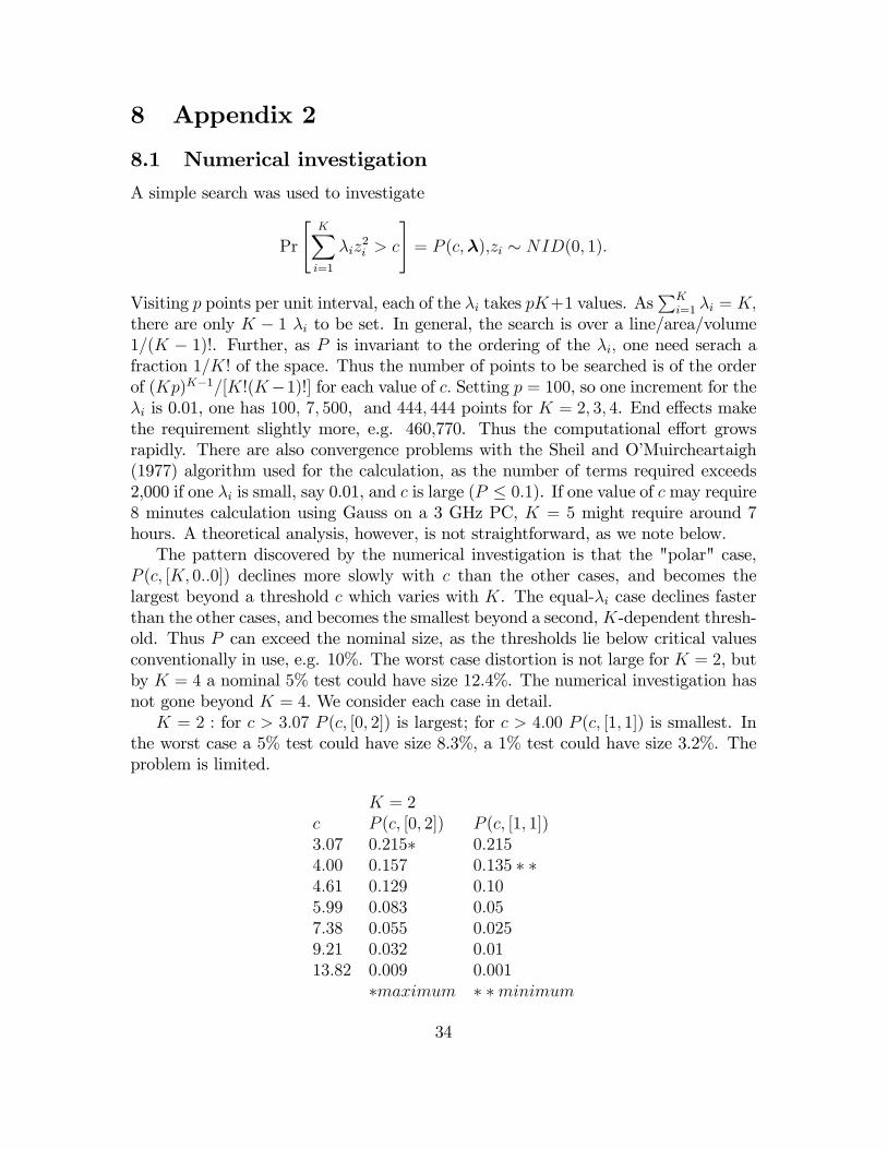
P (c; [K; 0::0]) declines more slowly with c than the other cases, and becomes thelargest beyond a threshold c which varies with K. The equal-�i case declines fasterthan the other cases, and becomes the smallest beyond a second,K-dependent thresh-old. Thus P can exceed the nominal size, as the thresholds lie below critical valuesconventionally in use, e.g. 10%. The worst case distortion is not large for K = 2, butby K = 4 a nominal 5% test could have size 12.4%. The numerical investigation hasnot gone beyond K = 4: We consider each case in detail.K = 2 : for c > 3:07 P (c; [0; 2]) is largest; for c > 4:00 P (c; [1; 1]) is smallest. In
the worst case a 5% test could have size 8.3%, a 1% test could have size 3.2%. Theproblem is limited.
K = 2c P (c; [0; 2]) P (c; [1; 1])3:07 0:215� 0:2154:00 0:157 0:135 � �4:61 0:129 0:105:99 0:083 0:057:38 0:055 0:0259:21 0:032 0:0113:82 0:009 0:001
�maximum � �minimum
34
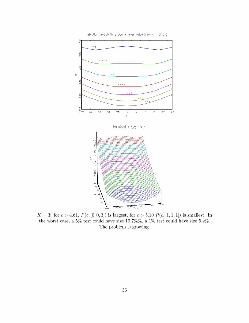
K = 3: for c > 4:61; P (c; [0; 0; 3]) is largest, for c > 5:10 P (c; [1; 1; 1]) is smallest. Inthe worst case, a 5% test could have size 10.7%%, a 1% test could have size 5.2%.
The problem is growing.
35
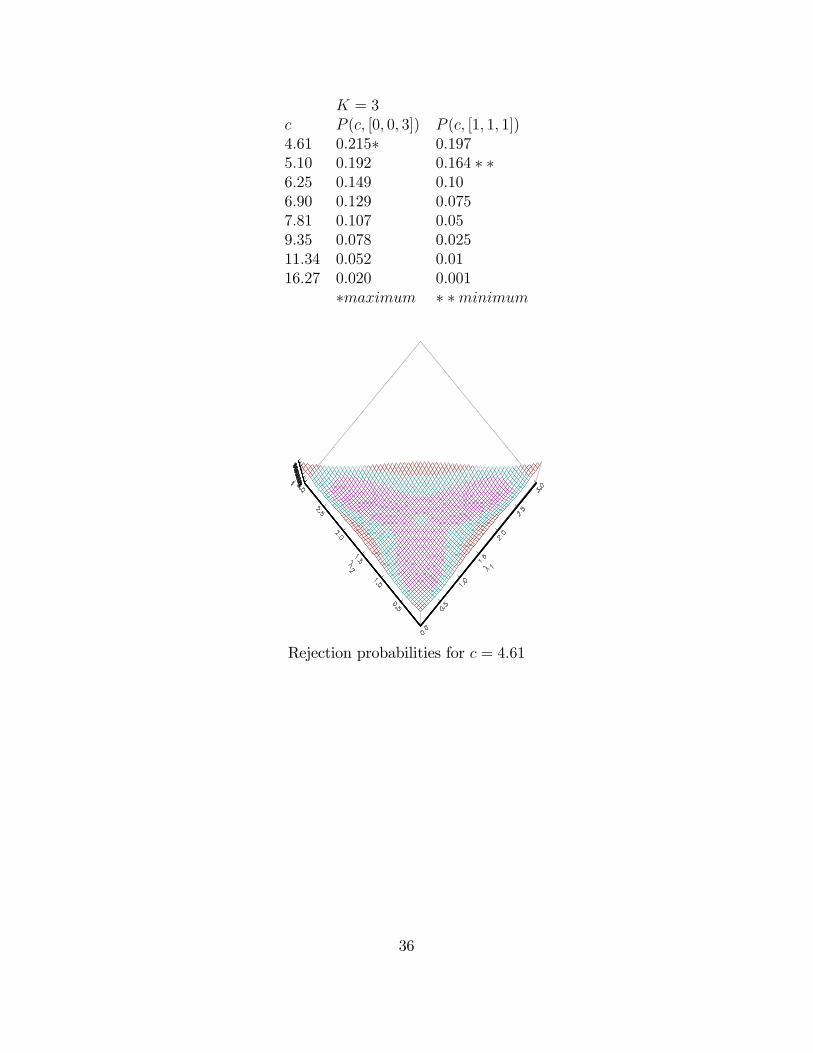
K = 3c P (c; [0; 0; 3]) P (c; [1; 1; 1])4:61 0:215� 0:1975:10 0:192 0:164 � �6:25 0:149 0:106:90 0:129 0:0757:81 0:107 0:059:35 0:078 0:02511:34 0:052 0:0116:27 0:020 0:001
�maximum � �minimum
Rejection probabilities for c = 4:61
36
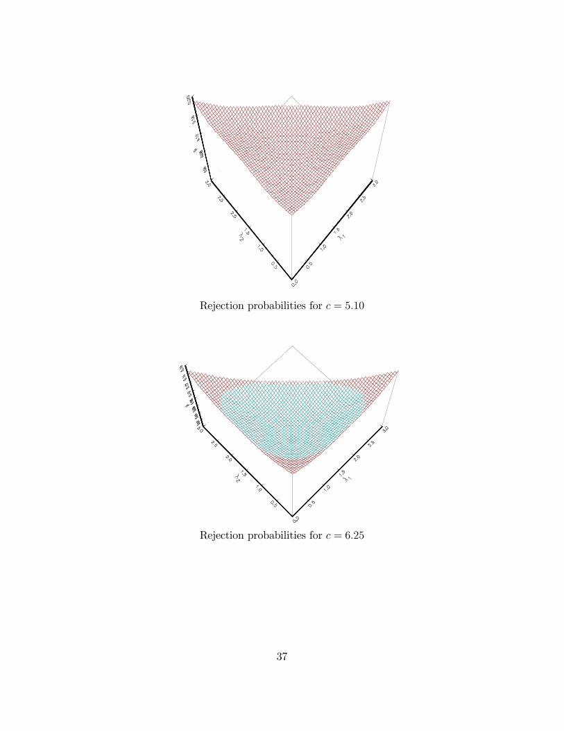
Rejection probabilities for c = 5:10
Rejection probabilities for c = 6:25
37

Rejection probabilities for c = 6:90
Rejection probabilities for c = 7:81
38
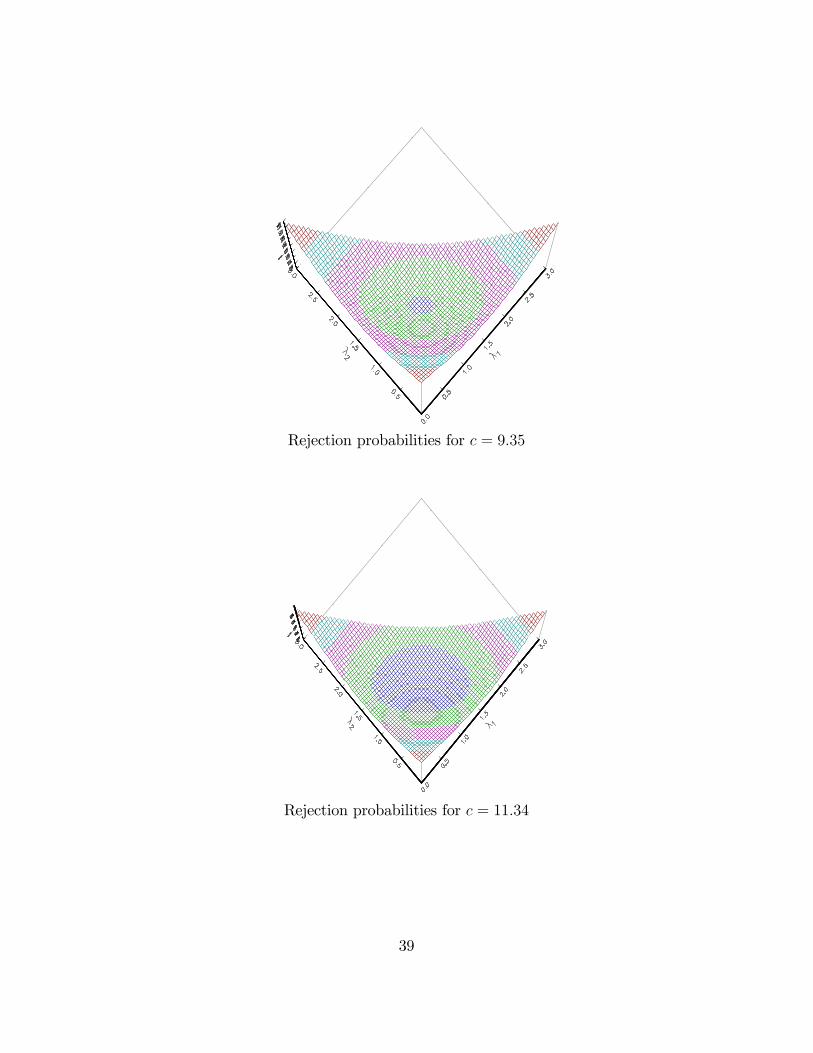
Rejection probabilities for c = 9:35
Rejection probabilities for c = 11:34
39

Rejection probabilities for c = 16:27
K = 4: for c > 6:15; P (c; [0; 0; 0; 4]) is largest, for c > 6:26 P (c; [1; 1; 1; 1]) issmallest. In the worst case, a 5% test could have size 12.4%%, a 1% test could havesize 6.8%. The problem continues to grow, and the worst cases begin to distort
inferences.K = 4
c P (c; [0; 0; 0; 4]) P (c; [1; 1; 1; 1])6:15 0:215� 0:1886:26 0:211 0:181 � �7:78 0:163 0:108:50 0:145 0:0759:49 0:124 0:0511:14 0:095 0:02513:28 0:068 0:0116:27 0:032 0:001
�maximum � �minimum
8.2 Analysis
If one considers a perturbation of the � vector from [�1; �2; �3; ::; �K ] to [�1+�; �2��; �3; ::; �K ], starting from � = [1; 1; ::; 1] on can visit every required point in �-space
40
in at most K steps. So one can �nd
@P (�;�;c)
@�=
1
2(�1 +�)2[cP (�;�;c)� � (�1 +�)P (�;�;c)]
� 1
2(�2 ��)2[cP (�;�;c)�� � (�2 ��)P (�;�;c)] :
In P , all �2 have 1 degree of freedom, in P � �1 multiplies a �2(3); as does �2 inP ��. As the P s are bounded, the derivative appears to diverge as �! �2: This mayor may not relate to the convergence problems noted above.
41
9 Appendix 3
We de�ne Between Groups and Within Groups estimators as usual:
b�BG =�X
0MX
��1X
0MY
b�WG =�X
0QX
��1X
0QY
where
Q = IN Q+;
Q+ = IT �1
Tii0;
M = IN M+;
M+ =1
Tii0= IT �Q+;
X =
26664X1
X2...XN
37775 ; Y =26664y1y2...yN
37775 ; Xi =
26664x0i1x0i2...x0iT
37775 ; yi =26664yi1yi2...yiT
37775 :Q+ is the matrix that transforms the data to deviations from the individual timemean, M+ is the matrix that transforms the data to averages.Suppose the true model is
yit = z0
it� + �i + vit; i = 1; :::; N; t = 1; :::; T
where z0it is a 1 �K vector of theoretical variables, �i � iid
�0; �2�
�; vit � iid (0; �2)
uncorrelated with the columns of zit and Cov (�i; vit) = 0: The observed variables are
xit = zit +mit;
where mit is a K � 1 measurement error uncorrelated with �i and vit: The estimatedmodel is
yit = x0
it� + �i + vit �m0it�; i = 1; :::; N; t = 1; :::; T:
In the case of exact measurement, mit = 0: So
yi = Xi� + �ii+ �i �Mi� = Xi� + � i;
say, where i is a column of T 1s,
�i =
26664vi1vi2...viT
37775 ;Mi =
26664m0i1
m0i2...m0iT
37775 :42
To consider the �generic�estimator, let
b�AG =�X
0AX
��1X
0AY
=
"NXi=1
X0
iA+Xi
#�1 NXi=1
X0
iA+yi
= � +
"NXi=1
X0
iA+Xi
#�1 NXi=1
X0
iA+� i;
where A = Q or M as appropriate, and
NXi=1
X0
iA+� i =
NXi=1
X0
iA+ [�ii+ �i �Mi�]
=NXi=1
[Zi +Mi]0A+ [�ii+ �i �Mi�] ;
where
Zi =
26664z0i1z0i2...z0iT
37775 :Given our assumptions,
E
"NXi=1
X0
iA+� i
#= �E
"NXi=1
M 0iA
+Mi�
#:
LetMi = [Mi1; ::;MiK ]
so the r � s�th element of M 0iA
+Mi has expectation
tr(E[M 0irA
+Mis]) = E[tr(MisM0irA)] = tr(�MrsITA) = �Mrstr(A)
if we assumemij are possibly correlated only contemporaneously within groups. Thus
E
"NXi=1
X0
iA+� i
#= �
"tr(A)
NXi=1
�M�
#= �tr(A)N�M�:
If we write
Xi = Zi +Mi
X0
iA+Xi = (Zi +Mi)
0A+(Zi +Mi) = Z0iA
+Zi + Z0iA
+Mi +M0iA
+Zi +M0iA
+Mi
43
and taking the Z as non-stochastic,
E(X0
iA+Xi) = Z
0iA
+Zi + E(M0iA
+Mi) = Z0iA
+Zi + tr(A)�M :
If we make appropriate assumptions about Zi to ensure that (1=N)PN
i=1 Z0iA
+Ziconverges to an appropriate limit, say �ZAZ ; then
b�AG = � +
"NXi=1
X0
iA+Xi
#�1 NXi=1
X0
iA+� i
p! � + p lim
"1
N
NXi=1
X0
iA+Xi
#�1p lim
1
N
NXi=1
X0
iA+� i
= � ���ZAZ + tr(A
+)�M��1
tr(A+)�M�:
For b�BG,A+ =M+ =
1
Tii0 ) tr(A) = 1
so b�BG p! � � [�ZMZ + �M ]�1�M�:
For b�WG;
A+ = Q+ = IT �1
Tii0 ) tr(A) = T � 1
so
b�WG
p! � � (T � 1) [�ZQZ + (T � 1)�M ]�1�M�= � � [�ZQZ=(T � 1) + �M ]�1�M�
These formulae are comparable, as �ZQZ grows with T: Indeed, if �ZQZ=(T � 1) ��ZMZ ; that is, the between sum of squares and the within sum of squares are roughlyproportional to the number of terms contributing to each, then
� = p lim(b�BG � b�WG) � 0:
We turn next to the estimation of the variance of the disturbances. For the genericestimation
b"AG = AY � AXb�AG = AY � AX �X 0AX
��1X
0AY;
Y = X� + �
where� =
�� 01; � � � � 0N
�0:
44
Substituting
b"AG = AX� + A� � AX�X
0AX
��1X
0A(X� + �)
= A� � AX�X
0AX
��1X
0A�:
Consider
b"0AGb"AG = � 0A� � � 0AX�X
0AX
��1X
0A�
=NXi=1
� 0iA+� i � � 0AX
�X
0AX
��1X
0A�:
AsA+� i = A
+ [�ii+ �i �Mi�] ;
1
N(T � 1)
NXi=1
� 0iA+� i
p! 1
T � 1��2�i
0A+i+tr(A+)f�2 + �0�M�g�:
If A+ = Q+ = IT � 1Tii0; tr(A+) = T � 1;
1
N(T � 1)
NXi=1
� 0iQ+� i
p! f�2 + �0�M�g:
If A+ =M+ = 1Tii0= IT �Q+; tr(A+) = 1;
1
N
NXi=1
� 0iM+� i
p!��2�i
0A+i+tr(A+)f�2 + �0�M�g�= T�2� + �
2 + �0�M�:
The other component in the �natural�variance estimate b"0AGb"AG=(N(T � 1)) is� 0AX
�X
0AX
��1X
0A�
We are assuming that (1=N)PN
i=1 Z0iA
+Zi converges to an appropriate limit, say�ZAZ ; and thus
1
N
NXi=1
X0
iA+Xi
p! �ZAZ + tr(A+)�M
Further, that
p lim1
N
NXi=1
X0
iA+� i = tr(A
+)�M�
45
Thus
1
N� 0AX
�X
0AX
��1X
0A� =
"1
N
NXi=1
X0
iA+� i
#0 "1
N
NXi=1
X0
iA+Xi
#�11
N
NXi=1
X0
iA+� i
p!�tr(A+)�M�
�0 ��ZAZ + tr(A
+)�M��1
tr(A+)�M�
= tr(A+)�0�M
�1
tr(A+)�ZAZ + �M
��1�M�
If A+ = Q+ = IT � 1Tii0; tr(A+) = T � 1;
1
N(T � 1)�0QX
�X
0QX
��1X
0Q�
p! �0�M
�1
(T � 1)�ZQZ + �M��1
�M�:
If A+ =M+ = 1Tii0= IT �Q+; tr(A+) = 1;
1
N� 0MX
�X
0MX
��1X
0M�
p! �0�M [�ZMZ + �M ]�1�M�:
Thus
1
N(T � 1)b"0WGb"WGp! f�2 + �0�M� � �0�M
�1
(T � 1)�ZQZ + �M��1
�M�g (25)
and1
Nb"0BGb"BG p! T�2� + �
2 + �0�M� � �0�M [�ZMZ + �M ]�1�M�: (26)
Finally, we require V ar(b�AG): We haveb�AG = � � ��ZAZ + tr(A+)�M��1 tr(A+)�M�:and thus under appropriate assumptions
pNhb�AG � � + ��ZAZ + tr(A+)�M��1 tr(A+)�M�i
D! N(0;��ZAZ + tr(A
+)�M��1 �
V ar
"1pN
(NXi=1
X0
iA+� i � tr(A+)�M�
)#��ZAZ + tr(A
+)�M��1):
AsNXi=1
X0
iA+� i =
NXi=1
[Zi +Mi]0A+ [�ii+ �i �Mi�] ;
E
"NXi=1
X0
iA+� i
#= �
"tr(A+)
NXi=1
�M�
#= �tr(A+)N�M�:
46
V ar
"NXi=1
X0
iA+� i
#= V ar
"NXi=1
[Z 0iA+ +M 0
iA+] [�ii+ �i �Mi�]
#
= V ar
"NXi=1
�Z 0iA
+�ii+Z0iA
+�i � Z 0iA+Mi�+M 0iA
+�ii+M0iA
+�i �M 0iA
+Mi�
�#where A+ = Q+ = IT � 1
Tii0or = M+ = 1
Tii0= IT � Q+: We are assuming no
correlation between groups. We thus need to evaluate
V ar(X0
iA+� i) = V ar
�Z 0iA
+�ii+Z0iA
+�i � Z 0iA+Mi�+M 0
iA+�ii+M
0iA
+�i �M 0iA
+Mi�
�= V ar[a+ b+ c+ d+ e+ f ]
say, whereE(X
0
iA+� i) = �tr(A+)�M� = E(f)
and if u is a random vector,
V ar(u) = E�[u�E(u)][u�E(u)]0
:
Thus
V ar(X0
iA+� i) = E(aa0) + E(bb0) + E(cc0)
+Cov(cf 0) + Cov(fc0) + E(dd0)
+E(ee0) + V ar(f):
asE(ad0) = �2�Z
0iA
+ii0A+E(Mi) = 0;
E(be0) = �2Z 0iA+E(Mi) = 0;
E(cd0) = E(�Z 0iA+Mi�v0iA
+Mi) = 0;
E(ce0) = E(�Z 0iA+Mi�i�iA+Mi) = 0;
E(de0) = E(M 0iA
+�ii�0iA
+Mi) = 0;
Cov(df 0) = Cov(M 0iA
+�ii;M0iA
+Mi�0) = 0;
andCov(ef 0) = E(M 0
iA+�i;M
0iA
+Mi�0) = 0;
assuming that the appropriate fourth order cross moments are zero, or, more strongly,that �i; �i; and Mi are independent. Of the 36 possible terms, 8 are non-zero, and 2of these are obtained by transposition. Further,
V ar(X0
iA+� i)
= �2�Z0iA
+ii0A+Zi + �2Z 0iA
+Zi + E(Z0iA
+Mi��0M 0
iA+Zi)
+Cov(cf 0) + Cov(fc0) + �2�E(M0iA
+ii0A+Mi) +
�2E(M 0iA
+Mi) + V ar(f)
47
We show below that
E(Z 0iA+Mi��
0M 0iA
+Zi) = �0�M�Z
0iA
+Zi
E(M 0iA
+Mi) = tr(A+)�M
E(M 0iA
+ii0A+Mi) = i0A+i�M
and that under assumptions of normality, that is if W is a matrix with i.i.d. rowsv N(0;�W )
V ar(W0AW�) = tr(A2) f�W��0�W + (�
0�W�)�Wg :Thus
V ar(f) = V ar(M 0iA
+Mi�)
= tr(A+2) f�M��0�M + (�0�M�)�Mg
Under these assumptions,
Cov(cf 0) = Cov(Z 0iA+Mi�;M
0iA
+Mi�) = 0:
Thus
V ar(X0
iA+� i)
= �2�Z0iA
+ii0A+Zi + �2Z 0iA
+Zi +
�0�M�Z0iA
+Zi + �2�i0A+i�M +
�2tr(A+)�M + tr(A+2) f�M��0�M + (�
0�M�)�Mg :Finally
pNhb�AG � � + ��ZAZ + tr(A+)�M��1 tr(A+)�M�i
D! N(0;��ZAZ + tr(A
+)�M��1 ��
T�2��ZAMAZ + (�2 + �0�M�)�ZAZ + �
2�i0A+i�M+
�2tr(A+)�M + tr(A+2) f�M��0�M + (�0�M�)�Mg
���
�ZAZ + tr(A+)�M
��1):
wherelimN!1
1
NZ 0iA
+ii0A+Z = T limN!1
1
NZ 0iA
+MA+Z
and A+ = Q+ = IT � 1Tii0or =M+ = 1
Tii0= IT �Q+: So
pNhb�WG � � + [�ZQZ=(T � 1) + �M ]
�1�M�i
D! N(0; [�ZQZ + (T � 1)�M ]�1 ��(�2 + �0�M�)�ZQZ+
�2(T � 1)�M + (T � 1) f�M��0�M + (�0�M�)�Mg
��
[�ZQZ + (T � 1)�M ]�1):
48
and the variance matrix can be written
[1=(T � 1)g [�ZQZ=(T � 1) + �M ]�1 ��(�2 + �0�M�)�ZQZ=(T � 1) + �2�M + f�M��0�M + (�0�M�)�Mg
��
[�ZQZ=(T � 1) + �M ]�1 :
ThuspNhb�BG � � + [�ZMZ + �M ]
�1�M�i
D! N(0; [�ZMZ + �M ]�1 ��
T�2��ZMZ + (�2 + �0�M�)�ZMZ + �
2�T�M+
�2�M + f�M��0�M + (�
0�M�)�Mg
��
[�ZMZ + �M ]�1):
To complete our analysis, and obtain the limiting variance of b�WG � b�BG, we needCov(b�WG
c; �BG): This would be zero except for the measurement error. Accordingly,we require only some terms of
Cov(X0
iM+� i; X
0
iQ+� i):
Remembering
X0
iA+� i
= [Z 0iA+ +M 0
iA+] [�ii+ �i �Mi�]
= Z 0iA+�ii+Z
0iA
+�i � Z 0iA+Mi� +M0iA
+�ii+M0iA
+�i �M 0iA
+Mi�
and as Q+ = IT � 1Tii0;M+ = 1
Tii0= IT �Q+;M+i = i;Q+i = 0;M+Q+ = 0; consider
X0
iM+� i
= Z 0i�ii+Z0iM
+�i � Z 0iM+Mi� +M0i�ii+M
0iM
+�i �M 0iM
+Mi�
= aM + bM+cM+dM+eM+fM , say
and
X0
iQ+� i
= Z 0iQ+�i � Z 0iQ+Mi�+M
0iQ
+�i �M 0iQ
+Mi�
= bQ+cQ+eQ+fQ, say.
Of the 24 possible covariances in Cov(X0iM
+� i; X0iQ
+� i); aM and dM have zero co-variance with X
0iQ
+� i under our assumption that �i is uncorrelated with �i and Mi;
Cov(bM ;bQ) = E(Z0iM
+�i(Z0iQ
+�i)0) = 0
49
as E(�i� 0i) = �2IT and M+Q+ = 0: Similarly Cov(bM ; eQ) = Cov(eM ;bQ) =Cov(eM ; eQ) = 0: Cov(bM ; cQ) = Cov(bM ; fQ) = Cov(eM ; cQ) = Cov(eM ; fQ) underour assumption that �i is uncorrelated withMi:Again, Cov(cM ;bQ) = Cov(cM ; eQ) =Cov(fM ;bQ) = Cov(fM ; eQ) = 0: This just leaves the 4 terms involving the measure-ment error,
Cov(cM ; cQ) = E(Z 0iM+Mi�(Z
0iQ
+Mi�)0)
Cov(cM ; fQ) = E(Z 0iM+Mi�(M
0iQ
+Mi�)0)
Cov(fM ; cQ) = E(M 0iM
+Mi�(Z0iQ
+Mi�)0)
Cov(fM ; fQ) = Cov(M 0iM
+Mi�;M0iQ
+Mi�)
Taking them in order, E(Mi��0Mi) has j; k-th element
E(m0i(j)�mi(k)�) = �
0E(mi(k)m0i(j))� = �j;k�
0�M�
where m0i(k) is the k-th row of Mi, and thus
Cov(cM ; cQ) = Z 0iM+E(Mi��
0Mi)Q+Zi)
0)
= �0�M�Z0iM
+ITQ+Zi)
0) = 0:
Cov(cM ; fQ) = E(Z 0iM+Mi��
0M 0iQ
+Mi)
= Z 0iM+E(Mi��
0M 0iQ
+Mi):
The expectation has j; k-th element
E(m0i(j)��
0M 0iQ
+mi(k))
= E(m0i(j)�m
0i(k)Q
+Mi)�
= E[(mi(j)m0i(k))
0(�Q+Mi�)
= EKXr=1
mi;j;r
KXs=1
mi;k;s
h�rq
+0(k)Mi�
i= E
KXr=1
�rmi;j;r
KXs=1
mi;k;s
TXt=1
q+kt
KXu=1
mi;t;u�u
= E
KXr=1
�r
TXt=1
q+kt
KXu=1
�u
KXs=1
mi;j;rmi;k;smi;t;u
usinga0bc0d = (a c)0(b d):
We are assuming all third order moments are zero, and thus this expectation will bezero, as will Cov(fM ; cQ): This leaves
Cov(fM ; fQ) = Cov(M0iM
+Mi�;M0iQ
+Mi�)
50
However, under assumptions of Normality, M+Q+ = 0 ensures that M 0iM
+Mi andM 0iQ
+Mi are independently distributed, and hence the covariance will be zero.We can now assemble the Hausman test statistic for the measurement error case.
One would calculate
h
= (b�WG � b�BG)0 hdV ar(b�WG) +dV ar(b�BG)i�1 (b�WG � b�BG)=
pN(b�WG � b�BG)0 hNdV ar(b�WG) +NdV ar(b�BG)i�1pN(b�WG � b�BG)NdV ar(b�WG)
= N1
N(T � 1)b"0WGb"WG
"NXi=1
X0
iQ+Xi
#�1
=1
N(T � 1)b"0WGb"WG
"1
N
NXi=1
X0
iQ+Xi
#�1p! f�2 + �0�M� � �0�M
�1
(T � 1)�ZQZ + �M��1
�M�g �
[�ZQZ + (T � 1)�M ]�1
NdV ar(b�BG)= N
1
Nb"0BGb"BG
"NXi=1
X0
iM+Xi
#�1
=1
Nb"0BGb"BG
"1
N
NXi=1
X0
iM+Xi
#�1p! fT�2� + �2 + �0�M� � �0�M [�ZMZ + �M ]
�1�M�g �[�ZMZ + �M ]
�1
using A+ = Q+ = IT � 1Tii0or =M+ = 1
Tii0= IT �Q+;
1
N
NXi=1
X0
iA+Xi
p! �ZAZ + tr(A+)�M
1
N(T � 1)b"0WGb"WG (27)
p! f�2 + �0�M� � �0�M�
1
(T � 1)�ZQZ + �M��1
�M�g (28)
51
1
Nb"0BGb"BG (29)
p! T�2� + �2 + �0�M� � �0�M [�ZMZ + �M ]
�1�M�: (30)
However, under the assumption that
[�ZQZ=(T � 1) + �M ]�1�M� = [�ZMZ + �M ]�1�M�
pN(b�WG � b�BG)
D! N(0; [1=(T � 1)g [�ZQZ=(T � 1) + �M ]�1 ��(�2 + �0�M�)�ZQZ=(T � 1) + �2�M + f�M��0�M + (�0�M�)�Mg
��
[�ZQZ=(T � 1) + �M ]�1 + [�ZMZ + �M ]�1 �
[�2��ZMZ + (�2 + �0�M�)�ZMZ + �
2�T�M + �
2�M + f�M��0�M + (�
0�M�)�Mg][�ZMZ + �M ]
�1):
9.1 A matrix result
If U is a random, K �K matrix, and � is a �xed K � 1 vector, V ar(U�) has i; i-thelement
V ar(u0(i)�) = �0V ar(u(i))�
if u0(i) is the i-th row of U: Similarly,V ar(U�) has i; j-th element
Cov(u0(i)�;u0(j)�) = �
0Cov(u(i);u(j))�:
Considering K = 2,
V ar(U�) =
��0 00 �0
� �V ar(u(1)) Cov(u(1);u(2))
Cov(u(2);u(1)) V ar(u(2))
� �� 00 �
�= (I2 �0)V ar(vec(U0))(I2 �)
Thus we can see that in general
V ar(U�) =(IK �0)V ar(vec(U0))(IK �)
So V ar((W0AW�) can be written in terms of V ar(vec(W0AW)), as A is symmetric.
9.2 Cov(Z0AW�;W0AW�)
This covariance matrix is given by
E(Z0AW��0W0AW) = Z0AE(W��0W0AW):
52
W��0W0AW has i-th row w0(i)��
0W0AW and thus i; j-th element
w0(i)��
0W0Awj =
KXl=1
wil�l
! KXm=1
�mw0mAwj
!
=
KXl=1
wil�l
! KXm=1
�m
TXt=1
TXs=1
wtmatswsj
!The product wilwtmwsj always has zero expectation, under the assumption that oddmoments of order 3 and 4 are zero.
9.3 E(Z 0A+M��0M 0A+Z)
E(Z 0A+M��0M 0A+Z) = Z 0iA+E(M��0M 0)A+Z
M��0M 0 has i; j-th element
m0(i)��
0m(j) =
"KXr=1
mir�r
#"KXs=1
mjs�s
#:
E(m0(i)��
0m(j)) = �ij
KXr=1
KXs=1
�Mrs�r�s = �ij�0�M�:
ThusE(Z 0A+M��0M 0A+Zi) = �
0�M�Z0A+Z
9.4 E(M 0A+M)
M 0A+M has i; j-th element
m0iA
+mj =TXt=1
TXs=1
mtiatsmsj;
E(m0iA
+mj) =
TXt=1
TXs=1
�tsats�Mij = �Mijtr(A+)
E(M 0A+M) = tr(A+)�M
9.5 E(M 0iA
+ii0A+Mi)
M 0A+ii0A+M is of the form M 0aa0M . Following the analysis for E(M 0A+M); weobtain
E(M 0aa0M) = tr(aa0)�M = a0a�M
E(M 0iA
+ii0A+Mi) = i0A+i�M
53
9.6 V ar(vec(W0AW)) and V ar(W0AW�) under Normality
Magnus and Neudecker (1988), p. 251, Theorem 12, provide, if x v N(0;); and Ais n� n; symmetric,
E(x0Ax) = tr(A)
V ar(x0Ax) = 2tr(AA) + 4�0AA�
We need to generalise this to a matrix normal W; of order T �K; but assume thatthe rows ofW are NID(0;�): The typical covariance required is Cov(w0iAwj; w
0rAws)
where wi is the i-th column of W: Consider
Qi;j =�w0i w0j
� � 0 AA 0
� �wiwj
�= 2w0iAwj:
As �wiwj
�v N(0;
��ii �ij�ij �jj
� IT )
V ar(Qi;j) = 2tr
"���0 11 0
� A
����ii �ij�ij �jj
� IT
��2#
= 2tr
"����ij �jj�ii �ij
� A
��2#
V ar(w0iAwj) =1
2tr
"��ij �jj�ii �ij
�2#tr(A2):
using (AB)(C D) = (AC) (BD); and tr(AB) = tr(A)tr(B): Consider next
Qi;j;r;s =�w0i w0j w0r w0s
� 26640 A 0 0A 0 0 00 0 0 A0 0 A 0
37752664wiwjwrws
3775 = 2w0iAwj + 2w0rAws:Now
V ar(Qi;j;r;s) = 4V ar(w0iAwj) + 4V ar(w
0rAws) + 8Cov(w
0iAwj; w
0rAws):
Applying our previous result
V ar(Qi;j;r;s) = 2tr
26648>><>>:0BB@26640 1 0 01 0 0 00 0 0 10 0 1 0
3775 A1CCA0BB@2664�ii �ij �ir �is�ij �jj �jr �js�ir �jr �rr �rs�is �js �rs �ss
3775 IT1CCA9>>=>>;23775
= 2tr
26642664�ij �jj �jr �js�ii �ij �ir �is�is �js �rs �ss�ir �jr �rr �rs
377523775 tr(A2)
54
Thus
Cov(w0iAwj; w0rAws) =
1
4tr(A2)
8>><>>:tr2664�ij �jj �jr �js�ii �ij �ir �is�is �js �rs �ss�ir �jr �rr �rs
37752
�tr �
�ij �jj�ii �ij
�2!� tr
��rs �ss�rr �rs
�2!):
In general,
tr
�B CC� D
�2!� tr(B2)� tr(C2)
= tr
��B CC� D
� �B CC� D
��� tr(B2)� tr(C2)
= tr
��B2 + CC� ?
? D2 + C�C
��� tr(B2)� tr(C2)
= tr(B2 + CC�) + tr(D2 + C�C)� tr(B2)� tr(C2)= tr(CC�) + tr(C�C) = 2tr(CC�):
In our case
CC� =
��jr �js�ir �is
� ��is �js�ir �jr
�=
��jr�is + �js�ir 2�jr�js
2�ir�is �jr�is + �js�ir
�Cov(w0iAwj; w
0rAws) = tr(A2) [�jr�is + �js�ir]
This can be veri�ed with some algebra, using x = [X1; ::; Xn]0 v N(0;))
E(XiXjXkXl) = !ij!kl + !ik!kl + !il!jk
(Anderson, 1958, p. 39). Our result also exhibits the necessary invariance to theordering of i; j; r; s: AsW 0AW has w0iAwj as i; j-th element, vec(W
0AW ) has i varyingmore rapidly than j, so if
k = n(j � 1) + i; l = n(s� 1) + r
then V ar(vec(W 0AW ) has k; l-th elementCov(w0iAwj; w0rAws) = tr(A
2) [�jr�is + �js�ir]If K = 2; the pattern of subscripts is266664i; jnl;m 1; 1 2; 1 1; 2 2; 21; 1 1; 1; 1; 1 + 1; 1; 1; 1 1; 2; 1; 1 + 1; 1; 1; 2 1; 1; 1; 2 + 1; 2; 1; 1 1; 2; 1; 2 + 1; 2; 1; 22; 1 1; 1; 2; 1 + 1; 1; 2; 1 1; 2; 2; 1 + 1; 1; 2; 2 1; 1; 2; 2 + 1; 2; 2; 1 1; 2; 2; 2 + 1; 2; 2; 21; 2 2; 1; 1; 1 + 2; 1; 1; 1 2; 2; 1; 1 + 2; 1; 1; 2 2; 1; 1; 2 + 2; 2; 1; 1 2; 2; 1; 2 + 2; 2; 1; 22; 2 2; 1; 2; 1 + 2; 1; 2; 1 2; 2; 2; 1 + 2; 1; 2; 2 2; 1; 2; 2 + 2; 2; 2; 1 2; 2; 2; 2 + 2; 2; 2; 2
377775 ;
55
and
V ar(vec(W0AW))
= tr(A2)
26642�21;1 2�1;1�1;2 2�1;2�1;1 2�21;2
2�1;1�2;1 �1;1�2;2 + �212 �1;1�2;2 + �
212 2�1;2�2;2
2�2;1�1;1 �1;1�2;2 + �212 �1;1�2;2 + �
212 2�2;2�1;2
2�21;2 2�2;1�2;2 2�2;2�2;1 2�22;2
3775 : (31)
We notice that the symmetry of W 0AW implies an implicit duplication in the vecoperator, and ensures that in the last array, column 2 = column 3 and row 2 = row3. Now stacking
Cov(w0iAwj; w0rAws) = tr(A
2) [�jr�is + �js�ir]
vertically, �rst on i; we have
Cov(W 0Awj; w0rAws) = tr(A
2) [�jr�s + �js�r]
then with respect to j;
Cov(vec(W 0AW ); w0rAws) = tr(A2) [�r �s + �s �r] :
where �r is the r-th column of �: Then we stack horizontally, �rst with respect to r,
Cov(vec(W 0AW );W 0Aws) = tr(A2) [� �s + �s �]
then with respect to s;
Cov(vec(W 0AW; vec(W 0AW )
= tr(A2)f�� �1 � � � � �K
�+ � �g
= V ar(vec(W 0AW )):
Finally, we need
V ar(W 0AW�)
= (IK �0)tr(A2)f�� �1 � � � � �K
�+ � �g(IK �)
= tr(A2)��� �0�1 � � � � �0�K
�+ � �0�
(IK �)
= tr(A2)��� �0�1 � � � � �0�K
�(IK �) + � (�0��)
= tr(A2)
���0�1 � � � � �0�K �
�(IK �) + � (�0��)
= tr(A2) f([�0�] �)(IK �) + � (�0��)g= tr(A2) f(�0�) ��) + (�0��)�g = tr(A2) f���0� + (�0��)�g :
Checking this for K = 2;
�=
��1�2
�;�=
��11 �12�12 �22
�;
56
and after some algebra
V ar(W 0AW�)
= tr(A2)
�2�21�
211 + 4�1�2�11�12 + �
22(�11�22 + �
212)
2�21�12�11 + �2�1(3�212 + �11�22) + 2�
22�12�22
2�21�12�11 + �2�1(3�212 + �11�22) + 2�
22�12�22
2�22�222 + 4�1�2�22�12 + �
21(�22�11 + �
212)
�which again can be obtained directly from (31).
57
0
5
10
15
20
25
30
35
40
45
50
55
60
65
70
75
80
85
90
95
100
0.00 0.10 0.20 0.30 0.40 0.50 0.60 0.70 0.80 0.90
corr
pow
er %
Htest HRtest
Figure 5: Power function comparison when N=25, T=4
10 Appendix 4
Power curves of the standard Hausman test (H-test) versus the simplest of the robustformulations presented in Section 2 (HR-test) plotted against corr for various samplesizes.
58
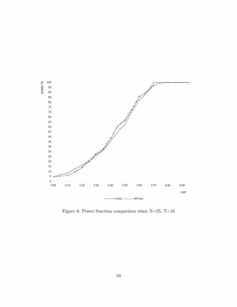
0
5
10
15
20
25
30
35
40
45
50
55
60
65
70
75
80
85
90
95
100
0.00 0.10 0.20 0.30 0.40 0.50 0.60 0.70 0.80 0.90
corr
pow
er %
Htest HRtest
Figure 6: Power function comparison when N=25, T=10
59
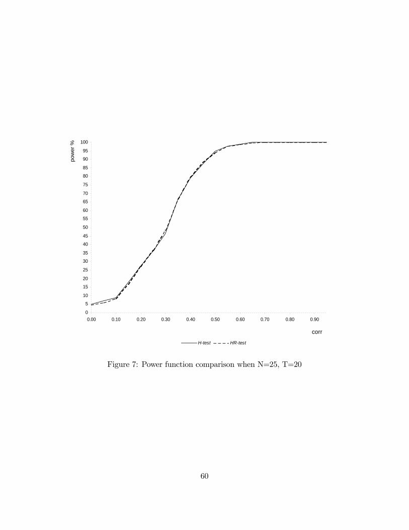
0
5
10
15
20
25
30
35
40
45
50
55
60
65
70
75
80
85
90
95
100
0.00 0.10 0.20 0.30 0.40 0.50 0.60 0.70 0.80 0.90
corr
pow
er %
Htest HRtest
Figure 7: Power function comparison when N=25, T=20
60
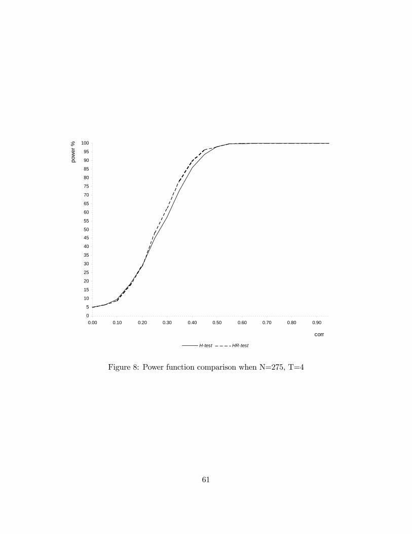
0
5
10
15
20
25
30
35
40
45
50
55
60
65
70
75
80
85
90
95
100
0.00 0.10 0.20 0.30 0.40 0.50 0.60 0.70 0.80 0.90
corr
pow
er %
Htest HRtest
Figure 8: Power function comparison when N=275, T=4
61
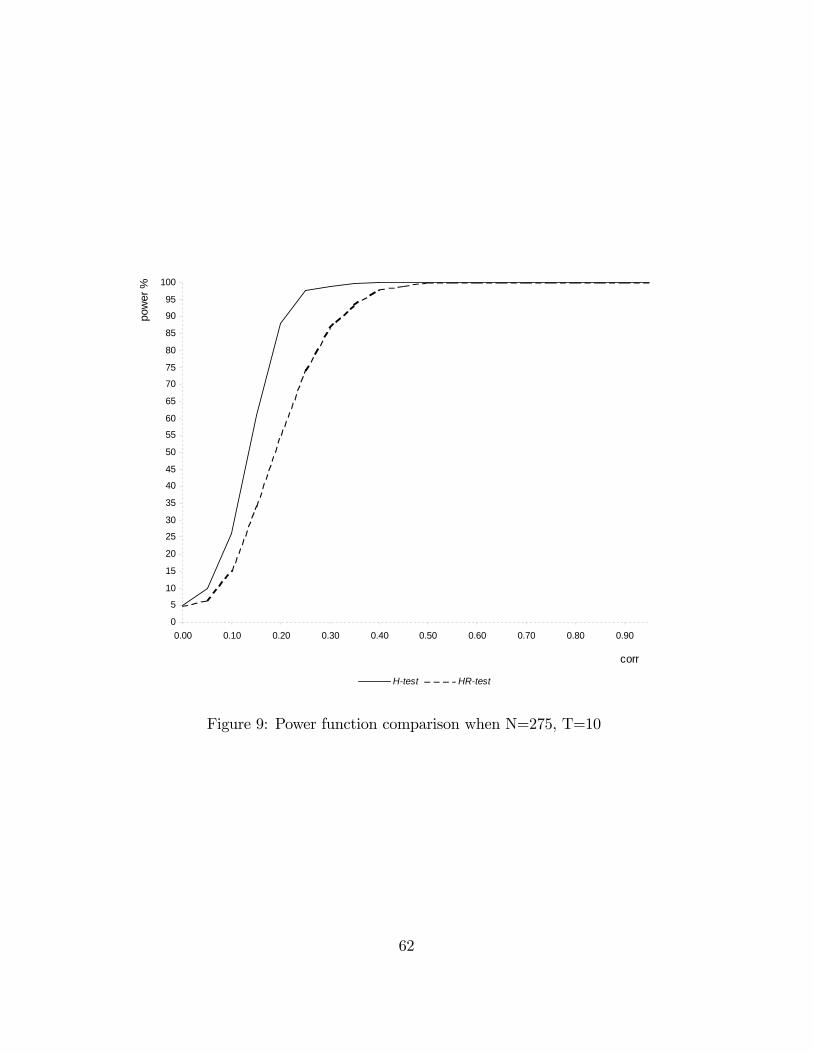
0
5
10
15
20
25
30
35
40
45
50
55
60
65
70
75
80
85
90
95
100
0.00 0.10 0.20 0.30 0.40 0.50 0.60 0.70 0.80 0.90
corr
pow
er %
Htest HRtest
Figure 9: Power function comparison when N=275, T=10
62
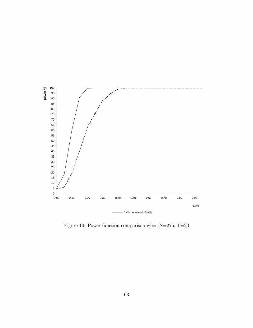
0
5
10
15
20
25
30
35
40
45
50
55
60
65
70
75
80
85
90
95
100
0.00 0.10 0.20 0.30 0.40 0.50 0.60 0.70 0.80 0.90
corr
pow
er %
Htest HRtest
Figure 10: Power function comparison when N=275, T=20
63