Embed Size (px)
Citation preview

0
UNIVERSITY OF CANTERBURY
Design-to-Resource (DTR) using
SMC Turbine Adaptive Strategy Design Process of Low Temperature Organic Rankine
Cycle (LT-ORC)
A thesis submitted in partial fulfilment of the requirements for the
Degree
Of Doctor of Philosophy in Mechanical Engineering
in the University of Canterbury
by Choon Seng Wong
University of Canterbury
2015

1
Supervisors
Prof. Susan Krumdieck Senior Thesis Supervisor, University of
Canterbury, NZ
Dr. Sid Becker Thesis Co-Supervisor, University of Canterbury,
NZ
Dr. Nicholas Baines Thesis Supervisory Committee Member/
Technical Consultant, NREC Concepts, UK
Special Acknowledgement to the following people in supporting the research
project and development of this thesis.
Assoc. Prof. Mark Jermy University of Canterbury, NZ
Assoc. Prof. Mathieu Sellier University of Canterbury, NZ
Dr. Don Clucas University of Canterbury, NZ
Dr. Boaz Habib Heavy Engineering Research Association, NZ
Jevon Priestly Allied Industrial Engineering, NZ
UC ORC Research Teams:
David Meyer, Leighton Taylor, Michael Southon, Ariff Ghazali
This author is funded by Heavy Engineering Educational & Research Foundation
(HEERF) in supporting this research project.

2
Contents Abstract __________________________________________________________________ 7
1.0 Introduction _________________________________________________________ 9
1.1 The Problem ___________________________________________________________ 10
1.2 Standard Design-to-Resource approach _____________________________________ 11
1.3 Design-to-Resource approach for low temperature ORC ________________________ 14
1.4 The Contribution ________________________________________________________ 16
1.4 SMC Adaptive Strategy ___________________________________________________ 19
1.5 Challenges in development of the SMC-DTR __________________________________ 20
1.6 Thesis Layout ___________________________________________________________ 21
1.7 References _____________________________________________________________ 23
Background _______________________________________________________________ 25
2.0 Literature Review ____________ 25
2.1 Background of Organic Rankine Cycle _______________________________________ 27
2.2 Selection of Working Fluid for ORC _________________________________________ 32
2.3 Industrial ORC Technology: A brief summary _________________________________ 39
2.4 State of the Art of ORC Turbines and Expanders _______________________________ 43
2.5 References _____________________________________________________________ 53
3.0 Thermodynamic Cycle Model ________________________________________ 63
3.1 Thermodynamic Analysis of an Organic Rankine Cycle __________________________ 65
3.1.1 Pre-heater and Evaporator Analysis________________________________________________ 66
3.1.2 Turbine Analysis _______________________________________________________________ 66
3.1.3 Condenser Analysis _____________________________________________________________ 67
3.1.4 Pump Analysis _________________________________________________________________ 67
3.1.5 Cycle Analysis _________________________________________________________________ 68
3.1.6 Numerical Model ______________________________________________________________ 69
3.2 Cycle Design Approach and Example ________________________________________ 71

3
3.3 References _____________________________________________________________ 77
3.4 References _____________________________________________________________ 77
4.0 Define Turbine Specification ________________________________________ 78
4.1 Introduction ___________________________________________________________ 80
4.2 Calculation of Shaft Speed and Turbine Diameter _____________________________ 82
4.3 Calculation of Number of Stages ___________________________________________ 83
4.4 Case Studies for Turbine/Expander Selection _________________________________ 86
4.5 Conclusion _____________________________________________________________ 88
4.6 References _____________________________________________________________ 89
Investigative Study _________________________________________________________ 90
5.0 Preliminary Design of Radial Inflow Turbine _______________________________ 90
5.1 Introduction ___________________________________________________________ 93
5.2 Standard Preliminary Design Approach ______________________________________ 95
5.2.1 Preliminary Design ________________________________________________________________ 96
5.2.2 Thermo-physical and Thermodynamic Properties _______________________________________ 99
5.2.3 Perfect Gas Model ________________________________________________________________ 99
5.2.4 Real Gas Model __________________________________________________________________ 101
5.2.5 Nozzle and Rotor Design __________________________________________________________ 104
5.2.6 Turbine Loss Model ______________________________________________________________ 106
5.2.7 Validation of Turbine Empirical Loss Model ___________________________________________ 110
5.2.8 Optimization of Objective Function __________________________________________________ 111
5.2.9 Numerical Mathematical Model ____________________________________________________ 112
5.3 Case Study for Low-Temperature Geothermal Brine __________________________ 113
5.4 Conclusion ____________________________________________________________ 120
5.5 References ____________________________________________________________ 121
Components of the SMC Adaptive Strategy ____________________________________ 123
6.0 Meanline Analysis of Radial Inflow Turbine ______________________________ 123
6.1 Introduction __________________________________________________________ 125
6.2 Turbine Loss Model _____________________________________________________ 127
4
6.3 Validation of Turbine Empirical Loss Model _________________________________ 131
6.4 References ____________________________________________________________ 133
7.0 CFD Analysis of Radial Inflow Turbine ___________________________________ 134
7.1 Introduction __________________________________________________________ 136
7.2 CFD Methodology ______________________________________________________ 138
7.2.1 Generation of Solid Models _____________________________________________________ 139
7.2.2 Meshing _____________________________________________________________________ 141
7.2.3 Details of Modelling the Physics _________________________________________________ 144
7.2.4 Solver _______________________________________________________________________ 148
7.3 Grid Independence Study ________________________________________________ 149
7.4 Validation of the CFD Model _____________________________________________ 151
7.5 Conclusion ____________________________________________________________ 152
7.6 References ____________________________________________________________ 153
8.0 Similarity Analysis _______________________________________ 154
8.1 Introduction __________________________________________________________ 156
8.2 Methodology _____________________________________________________________ 158
8.2.1 Similarity Analysis _____________________________________________________________ 159
8.2.2 Scaling Approach for Different Compressible Fluids __________________________________ 160
8.2.3 Evaluation of Aerodynamic Performance using CFD Analysis ___________________________ 161
8.3 Result ________________________________________________________________ 163
8.4 Discussion ____________________________________________________________ 169
8.5 Conclusion ____________________________________________________________ 178
8.6 References ____________________________________________________________ 179
Application of the SMC-DTR Approaches ______________________________________ 181
9.0 Application of the SMC-DTR using Meanline Analysis ______________________ 181
9.1 Introduction __________________________________________________________ 183
9.2 Application of the SMC-DTR approach in a waste heat recovery (WHR) system _____ 186
9.2.1 Heat source and heat sink: ______________________________________________________ 186
9.2.2 Cycle design and fluid selection: _________________________________________________ 186

5
9.2.3 Define turbine specification: ____________________________________________________ 187
9.2.4 Matching existing turbines: _____________________________________________________ 188
9.2.5 Design of Nozzle Vanes: ________________________________________________________ 189
9.2.6 Application of the SMC adaptive strategy __________________________________________ 191
9.2.6 Mechanical design and system integration: ________________________________________ 196
9.3 Conclusion ____________________________________________________________ 201
9.4 References ____________________________________________________________ 202
10.0 Application of the SMC-DTR using CFD Analysis on Turbine with Fix Nozzle Vane 204
10.1 Introduction _____________________________________________________________ 206
10.2 Application of the SMC-DTR Approach to Design an Air-Cooled Binary Plant _______ 209
10.2.1 Heat source and heat sink ____________________________________________________ 210
10.2.2 Cycle design and fluid selection _______________________________________________ 211
10.2.3 Define turbine specification: __________________________________________________ 212
10.2.4 Matching existing turbines: ___________________________________________________ 213
10.2.5 Application of the SMC Adaptive Strategy _______________________________________ 213
10.3 Conclusion ____________________________________________________________ 225
10.4 References ____________________________________________________________ 227
11.0 Application of the SMC-DTR using CFD Analysis on Turbine with Variable Nozzle
Vane ______________________________________ 228
11.1 Introduction __________________________________________________________ 230
11.2 Test Subject – Automotive Turbocharger with Variable Nozzle Vanes ____________ 232
11.3 Performance Optimization using Variable Nozzle Vanes _______________________ 233
11.4 Application of the SMC-DTR Approach in Heat Source with Variable Mass Flow ____ 241
11.4.1 ORC System _______________________________________________________________ 241
11.4.2 Application of the SMC Adaptive Strategy _______________________________________ 243
11.5 Discussion – Performance Evaluation of Variable Nozzle Vanes _________________ 247
11.6 Conclusion ____________________________________________________________ 251
11.7 References ____________________________________________________________ 252
12.0 Conclusion _________________________________________________________ 253
12.1 Summary _____________________________________________________________ 254

6
12.1.1 Background _______________________________________________________________ 254
12.1.2 Investigative Study _________________________________________________________ 255
12.1.3 Components of the SMC Adaptive Strategy______________________________________ 255
12.1.4 Application of the SMC-DTR Approaches ________________________________________ 257
12.2 Perspectives __________________________________________________________ 260

7
Abstract
Low grade heat source has a huge amount of power generation potential from the
industrial waste heat, and the untapped low temperature geothermal reservoirs. A suitable
turbine for these heat resources is usually not available from the market. A turbine can be
designed and developed but it requires the knowledge based engineering (KBE) in the turbine
technology with high engineering development cost. It is not cost effective to follow the
conventional turbine design and development pattern for each set of working fluid and
operating condition for ORC system. Another solution is to select and adapt the off-the-shelf
turbines for the given heat resources. The objective of this thesis is to define and develop the
design-to-resource (DTR) methodology coupled with the SMC turbine adaptive strategy,
named SMC-DTR approach. . The SMC strategy consists of three different analysis techniques;
similarity analysis, meanline analysis, and computational fluid dynamics (CFD) method, to
analyse the turbine performance for application and working fluid different from the original
design. This strategy allows the design and optimization of an ORC system for low temperature
resources by adapting the off-the-shelf radial inflow turbines for various heat resource
condition.
The SMC-DTR approach was applied in three different resources condition. The
numerical study shows that the off-the-shelf radial inflow turbines are feasible to be adapted as
ORC turbines but the turbine efficiency would deteriorate. The performance of automotive
turbocharges deteriorates up to 20% whereas the gas turbine performance changes up to 10%
if the working fluid is changed from air to refrigerants, including R134a, R245fa, and
isobutane. Most of the off-the-shelf turbines are designed for sub-sonic expansion. If they are
used for supersonic expansion, the turbine efficiency deteriorates when the expansion ratio
increases. The rotor blade passage chokes, and the flow accelerates downstream of the rotor
throat. This leads to the high swirl angle at the turbine outlet and high turbine loss in term of
kinetic energy, which is reflected in the low turbine efficiency.
The application of the SMC-DTR approach also shows that a radial inflow turbine with
fixed nozzle vanes can be selected and adapted for two different resource condition: constant
heat source and heat sink condition, and constant heat source condition with varying heat sink
temperature. The turbine efficiency and the thermal efficiency of the thermodynamic cycle

8
change up to 2% when the heat sink temperature changes from 10 to 23°C. However, a radial
turbine with fixed nozzle vanes is not suitable for the heat source with varying flow rate. If the
mass flow is reduced by 25% off the design value, the turbine performance and the
thermodynamic cycle performance drop significantly. A variable nozzle turbine has to be
selected for adaptation for the heat source with varying mass flow for optimal performance.
The thesis also evaluated the suitability of off-the-shelf turbines as ORC turbine and
proposed a number of design changes. Automotive turbochargers and gas turbines cannot be
applied directly as the ORC turbines since they are originally designed for air. A mechanical
system design has to be performed to be used with refrigerants.

9
1.0 Introduction
This chapter describes the key contribution from this thesis work, provides the context of the
contribution in the field, and gives the thesis organization. Geothermal energy is a promising
low-carbon energy resource. The major technical barrier to expanded power generation from
low-temperature resources is the lack of available expansion machines (or turbines). There is
a growing body of literature describing thermodynamic cycle analysis, organic working fluids
and component design for organic Rankine cycle (ORC) energy converters. If it was possible
to simply order an expansion machine or a turbine for a given mass flow, expansion ratio and
working fluid from a manufacturer, then the plant development cost would be the only barrier.
Many of the early experimental sub-MW ORC researchers used positive displacement devices
such as scrolls and screws. There are many developmental challenges and limitations with
positive displacement machines, but they pale in comparison to the work of developing a
turbine. The axial steam turbine is the work-horse of power generation, and large-scale
geothermal power systems rely on commercially developed axial turbines for both flash steam
plant, and binary ORC plant. The axial turbine is scalable and versatile, but its application is
limited in the small scale and low-temperature range.
It is possible to develop a radial turbine for a given application through the standard R&D
process. However, the cost of developing one turbine for one condition and one working fluid
is far in excess of research funding available in New Zealand. The strategy explored in this
thesis is to analyse and adapt existing radial inflow turbines for an organic working fluid and
pressure ratio for the thermodynamic cycle best suited to a particular resource. The strategy
would utilize the radial turbine for a different application and working fluid than the original
design. The key contribution in this thesis is the development and demonstration of the turbine
analysis strategy for the SMC turbine adaptation approach. The SMC approach makes strategic
use of Similarity, Meanline and Computational Fluid Dynamics analyses, and is integrated to
the proposed design-to-resource (DTR) method for low temperature resources to form SMC-
DTR approach.

10
1.1 The Problem
A geothermal resource can be exploited by matching the resource to an existing power
conversion system (such as Ormat Energy Convertor) [1], or by designing a power conversion
system based on the given resource. Power conversion units are commercially available for
high temperature resources; steam-based Rankine cycle from General Electric (GE) and an
organic Rankine cycle using n-Pentane as working fluid from Ormat [1]. The commercially
available systems have been developed over many years, specifically with one working fluid
and one turbine design that can be scaled to different power range by increasing the number of
stages. The problem is the large amount of research funding and development time needed to
develop ORC systems based on other working fluids for use in lower temperature ranges. It is
not practical to follow the historical pattern of research and experimental development,
particularly in New Zealand with limited research funding support for fundamental Mechanical
Engineering science that would be needed for development of a radial turbine for an organic
working fluid. This thesis proposes a way to explore the possible adaptation of existing turbines
to ORC applications using the modern turbine design and analysis tools.

11
1.2 Standard Design-to-Resource approach
The low temperature resources require a design of the energy conversion system that is
different to the high temperature resources in two aspects:
1) Organic Rankine cycle has a higher thermal efficiency than a conventional steam-based
Rankine cycle for low temperature resources [2]. However, the energy conversion
system has to be designed and handled with care as all organic working fluids are costly
and either flammable, toxic or having high greenhouse gas potential [3].
2) Multi-stage axial turbine is commonly used for steam Rankine cycle with high resource
temperature [4]. However, different types of turbines are better match for the pressure
ratio and working fluid for the low temperature resources, such as radial inflow turbine
[5-8], radial outflow turbine [9], scroll expander [10], and screw expander [11, 12].
An organic Rankine cycle for low temperature resources can be designed and developed using
the standard design-to-resource (DTR) approach, as illustrated in Figure 1.1. A thermodynamic
model of an organic Rankine cycle is designed based on the given heat resource and heat sink
condition, by applying rules for heat exchanger pinch-points, degree of superheat, maximum
pressure, and critical temperature of the working fluid. A parametric study is performed to
select the optimal working fluid for maximum cycle efficiency. The type of the system
components are selected to match the heat transfer requirements and pump conditions. The
individual components would need to be designed, developed, and tested in the OEC system.
All the components (heat exchangers and turbine) are assembled and a field test is performed.

12
Figure 1.1: Standard DTR approach for low temperature resources
The standard DTR approach for commercial development of low temperature resources
would only be successful if turbines were available in the market for the working fluids used
in the binary power plant. The conventional turbine design and development approach is
illustrated in Figure 1.2 [13]. An iterative cycle of in-depth engineering design and analysis
steps are required. Preliminary design means matching the available pressure drop, mass flow,
and inlet and exit enthalpies to the desired turbine speed and turbine principal geometry to
achieve the best efficiency. The detailed design investigations include aerodynamic design of
blade profile, finite element analysis (FEA) on structural integrity of the blade, computational
fluid dynamics (CFD) analysis on aerodynamic performance, rotor-dynamic analysis, and
system integration of turbine and auxiliary components. The resulting turbomachine design is
then embodied by manufacture of prototype, and laboratory testing. The testing results feed
Heat resource & heat sink
Cycle design & fluid
selection
Selection of vaporizer and
condenser types
Design and development
of heat exchanger
Components’ testing
System assembly
Field test of power plant
Selection of turbine’s
types
Design and development
of turbine (Figure 1.2)

13
back into the design and the design cycle proceeds with the objective of improving the design
of the next generation of turbines.
Figure 1.2: Standard turbine design and development approach [13]
Each step of the process requires in-depth engineering knowledge and experience, also
known as knowledge-based engineering (KBE). Jet engines for airliners and steam turbines for
power plants continue to undergo research and development cycles to improve efficiency and
reliability. Mass-manufactured turbomachines in consumer products like vacuum cleaners,
fans and pumps also require KBE and investment in R&D to achieve cost targets. The thing
that all of the conventional turbomachines have in common, is that they represent further
development of existing turbines for the same working fluid under similar working conditions.
The challenge for ORC development is the lack of this existing platform for expander
technology using organic fluids for power generation. Ormat is a successful geothermal power
plant developer because they have essentially built up their own KBE and axial turbine design
platform for pentane. Ormat can then design the Ormat energy converter (OEC) unit to suit a
range of high temperature resource situations. Thus, the conventional DTR approach is to use
an existing design platform and scale the size of the existing technology to optimize a given
resource.

14
1.3 Design-to-Resource approach for low temperature ORC
The design and development of a turbine for low temperature resources with low
potential power output entails a high investment cost, and a high capital cost per kilowatt hour,
attributed to the complexity of the aforementioned process and low amount of power
generation. Thus, low temperature ORC (LTORC) developers have focused on using
turbomachine technology developed for refrigerants. Given the lower generation potential of
LTORC, leveraging an existing technology is a logical approach.
a. Scroll compressors have been adapted as scroll expanders for micro-scale ORC system
with potential power output of a few kilowatts [14-19].
b. The feasibility of adapting different positive displacement machines have been studied,
including vane expander and piston expander (reported in a review by Bao [20]) using
organic working fluids for power conversion system less than 100 kW.
c. A refrigeration system has been re-purposed by replacing the centrifugal impeller with
a radial inflow turbine, and changing the working fluid from R245fa to R134a to match
the heat source condition [21-23].
d. A turbocharger using air as working medium has been re-purposed as an ORC turbine
using organic working medium [24], but no details are found regarding the adaptation
strategy and the turbine performance.
Among these adaptive solutions, the conversion of scroll compressors into scroll expanders
allows the development of the small scale power conversion units with potential power output
up to 30 kW [25]. The conversion of other positive displacement machines such as the vane
expander and piston expander results in a low turbine efficiency of less than 70% [20], and the
converted machines are limited to small power conversion units with less than a few hundred
kilowatts. The repurposing of a refrigeration system can reduce the investment cost but a
turbine has to be designed using the conventional turbine design and analysis approach [21].
The repurposing of a turbocharger as an ORC turbine using different working fluid is an
interesting concept. This approach reduces the investment cost and allows the design and build
of energy conversion units without necessitating a strong KBE in turbine technology. However,
the one known project was reported by Barber Nichols for a US Military project, and no details
were available regarding the adaptation process, analysis strategy, and the performance of the
adapted turbines.

15
The gap to be filled by the work in this thesis is the lack of strategy to analyse and adapt
existing radial inflow turbines for working fluid and application different from the original
design. In this thesis, the existing turbines investigated are commercially available off-the-shelf
turbines which do not require custom manufacturer. The selection of a suitable turbine from
the existing turbines is carried out to match the resource condition or to match the cycle design.
The adaptation of the turbine is defined as the utilization of turbine nozzle and rotor, and
modification of mechanical system design (re-design the casing, re-design the lubrication
system, and re-select the bearing) for a different working fluid and application. The turbine
adaptation approach covers only one type of turbine, a radial inflow air or gas turbine. Other
types of turbines, such as axial turbine, radial outflow turbine, and positive displacement
machines are not considered in this thesis research, but could also be investigated using the
proposed adaptation approach. The radial inflow turbine is selected as the core subject of the
adaptation approach for the following reasons:
a. Radial inflow turbine is suitable for energy conversion units with a wide range of
potential power output, from a few kilowatts to a few megawatts [25].
b. Radial inflow turbine is suitable for low temperature resources with a lower system
pressure ratio than high temperature resources.
c. Radial inflow turbine shows a higher isentropic efficiency than positive displacement
machines.
d. Radial inflow turbine is relatively simple to manufacture and assemble compared to the
multi-stage axial turbine.
e. Radial inflow turbines are commercially available in different geometry and size as
automotive turbochargers and micro gas turbines with a lower price tag, compared to
commercially available steam turbines.
The strategy of the turbine adaptation approach and the questions to be addressed are presented
in detail in the subsequent section.

16
1.4 The Contribution
The contribution of this thesis is engineering gap for adaptation of existing radial inflow
turbines for working fluid different from the original design. Up to the time of writing this
thesis, no open literature was found regarding the analysis and adaptation of existing turbines
to different working fluids (except the publications by the author). The turbine analysis strategy
is named the SMC adaptation strategy, where S refers to similarity analysis, M refers to
meanline analysis, and C refers to computational fluid dynamic (CFD) analysis. The SMC
approach is needed because the standard approach is not possible given research investment
constraints. The SMC turbine adaptation strategy forms the backbone of the new iterative
LTORC design-to-resource (DTR) method developed in this thesis. The new DTR method with
integrated SMC analysis is named SMC-DTR, and illustrated in Figure 1.3.
The SMC-DTR turbine adaptation approach includes:
a. Define turbine specification.
b. Matching existing turbines to the heat resources
c. SMC adaptive strategy
d. Mechanical design and system integration
e. Laboratory testing
The SMC adaptive strategy allows the engineers to study the performance of existing turbines
for the working fluid determined from the cycle design, and match the turbines to different
resources. If the turbine efficiency using the working fluid from the cycle design does not fall
within an acceptable range, the calculation process is repeated using another working fluid or
another turbine, as shown in Figure 1.3. Only the process enclosed in the dotted box is
presented in this thesis. The differences between the new DTR and the standard DTR approach
are presented in Table 1.1.

17
Table 1.1: Differences between the standard DTR and new DTR methods
Standard DTR approach New DTR approach
Turbine development
strategy
Turbine is designed using the
turbine design wheel in
Figure 1.2.
Existing radial gas turbine is
selected and adapted to the
cycle design.
Numerical calculation Forward analysis. The turbine
is designed based on the
working fluid.
Iterative analysis. Different
turbines can be analysed
using the SMC approach for
different working fluid to
optimize the cycle
performance.

18
Figure 1.3: SMC-DTR approach for low temperature resources
Heat resource & heat sink
Cycle design & fluid
selection
Selection of vaporizer and
condenser types
Design and development
of heat exchanger
Components testing
System assembly
Field test of power plant
Define turbine
specification
Matching existing
turbines (rotor, or nozzle
and rotor)
SMC Strategy
Mechanical design and
system integration
Laboratory testing
Turbine Adaptation Process

19
1.4 SMC Adaptive Strategy
The SMC adaptive strategy involves three turbine analysis techniques; similarity
analysis, meanline analysis, and CFD analysis. The SMC strategy is unique because the turbine
performance is investigated using the most relevant and informative analysis for the given
situation. The similarity analysis is performed only if the turbine performance map is available.
If the turbine performance map is not available, the meanline analysis is performed. The turbine
efficiency using the selected working fluid is evaluated using either the similarity analysis or
the meanline analysis. If the turbine efficiency does not fall into an acceptable range, the
working fluid can be re-selected from the cycle design, or the turbine can be re-selected. The
CFD analysis is performed if the efficiency of the selected turbine is acceptable, or there is
only one available turbine. The decision flow chart of the SMC approach is illustrated in Figure
1.4.
Figure 1.4: SMC analysis approach
Similarity Analysis
Meanline Analysis
CFD Analysis
1
2
3
Mechanical design
Selection of Turbine
η is acceptable?
Yes
No
Cycle design (re-select fluid) or turbine
selection (re-select existing turbines)
1: Turbine performance map (using air as working medium) is available.
2: Turbine performance map is not available.
3: Only one existing turbine is available.

20
1.5 Challenges in development of the SMC-DTR
A number of research works are required to address the following issues in order to
complete the SMC-DTR approach.
a. A turbine is typically designed for a specific set of working fluid and operating
condition. Is it feasible to adapt existing gas turbines for organic working fluid?
b. What components of a radial gas turbine can be retained and what components have to
be re-designed if the working fluid is changed from air to organic working fluid, such
as isobutane or R245fa?
c. A turbine preliminary design approach can be used to select an existing turbine with
the closest dimension and geometry to the design output from the preliminary design.
The turbine preliminary design approach has been developed using ideal gas law
assuming constant isobaric specific heat [26], before the work of this thesis is
performed. What is the difference in the design output from the preliminary design
approach using different gas models (ideal gas and real gas model)?
d. Similarity analysis can scale a turbine from one operating condition to another, and
scale a turbine for different turbine diameter if the working fluid is the same [27].
However, similarity analysis cannot scale a turbine from one working fluid to another,
especially if the working fluid is compressible. What is the appropriate assumption or
approach to perform the similarity analysis for different working fluid?
e. How to optimize the cycle performance using the adapted turbines if the resource
condition is changing?
The aforementioned challenges were successfully investigated in this thesis. The main
components of the SMC analysis approach were investigated and applied separately for each
case study, in order to exhibit the feasibility of the components as standalone analysis
approaches.

21
1.6 Thesis Layout
The aim of this thesis is to develop the SMC-DTR approach for low temperature resources with
different resources’ behaviour, and the main contribution of this thesis is to develop the key
component, SMC analysis approach.
Background
Chapter 2 presents the literature review of organic Rankine cycle (ORC) as the key technology
in energy conversion units for low temperature resources. The literature review covers the
background of ORC, selection of working fluid, development of the industrial ORC units, and
state of the art of turbines and expanders.
Chapter 3 presents the numerical calculation of the standard thermodynamic modelling of the
ORC system using Engineering Equation Solver (EES), an essential component of the SMC-
DTR approach. This component is coupled to the SMC adaptive strategy to optimize the cycle
performance. This component allows the engineers to select the working fluid and determine
the turbine operating condition for maximum system performance.
Chapter 4 presents the standard approach to define the turbine specification: calculating the
shaft speed, turbine wheel diameter, and number of stage using a standard turbine specific
speed-specific diameter performance chart.
Investigative Study
Chapter 5 presents the radial inflow turbine preliminary design method. This component
allows the users to match existing turbines to the cycle design with different working fluid. The
turbine designed using ideal gas model (with constant specific heat) and real gas model are
compared.
Components of the SMC Approach
Chapter 6 presents the meanline analysis of radial inflow turbine and the model validation.
Chapter 7 presents the CFD method in analysing a radial inflow turbine using ANSYS
Turbomachinery software. An industrial gas turbine is presented to validate the CFD model.

22
Chapter 8 presents the similarity analysis approach to scale a turbine from air (behaves as
ideal gas) to organic working fluid (behaves as real gas). Three different variable parameter
sets are established and investigated, known as perfect gas approach, variable pressure ratio
approach, and constant specific speed approach. The most feasible and accurate approach are
selected and applied in the similarity analysis component in the SMC approach. An industrial
gas turbine is selected as the test subject in this chapter. A correction chart is developed to
extend the application of the selected approach for different pressure ratio.
Application of SMC-DTR approach
Chapter 9 presents the application of the SMC-DTR approach for two nozzle-less automotive
turbochargers without the turbine performance map in designing the ORC system. This chapter
presents the cycle design and fluid section, calculation of the turbine specification, meanline
analysis of the SMC adaptive strategy, and the mechanical system design to adapt the
automotive turbochargers into ORC turbines.
Chapter 10 presents the application of a radial gas turbine with fixed nozzle vanes using the
SMC-DTR approach for a resource condition with constant heat source condition and varying
heat sink temperature. The CFD analysis of the SMC adaptive strategy is applied to evaluate
the turbine performance, and the flow field across the turbine blade passage was compared for
different working fluids.
Chapter 11 presents the application of a variable nozzle turbocharger using the SMC-DTR
approach for a resource condition with constant heat sink temperature and varying heat source
flow rate. The first section presents the investigate study to optimize the turbine performance
using variable nozzle vanes. The second section demonstrates the application of the SMC-DTR
approach to optimize the cycle performance. The third section discusses the losses within the
variable nozzle vanes at different vane angle.
Conclusion
Chapter 12 presents the summary and the implications of the lessons from each section, and
the author’s perspective of this research work.

23
1.7 References
1. Nasir, P., et al., Utilization of Turbine Waste Heat to Generate Electric Power at
Neptune Plant. 2004.
2. Vankeirsbilck, I., et al., Organic rankine cycle as efficient alternative to steam cycle for
small scale power generation. Proceedings of 8 th International Conference on Heat
Transfer, Fluid Mechanics and Thermodynamics, Pointe Aux Piments (Mauritius),
2011.
3. Chen, H., D.Y. Goswami, and E.K. Stefanakos, A review of thermodynamic cycles and
working fluids for the conversion of low-grade heat. Renewable and Sustainable Energy
Reviews, 2010. 14(9): p. 3059-3067.
4. Meher-Homji, C.B. ‘The Historical Evolution of Turbomachinery. in Proceedings of
the 29th Turbomachinery Symposium, Texas A&M University, Houston, TX. 2000.
5. Clemente, S., et al., Bottoming organic Rankine cycle for a small scale gas turbine: A
comparison of different solutions. Applied Energy, 2013. 106: p. 355-364.
6. Agahi, R. Application of an Inflow Radial Turbine in a Geothermal Organic Rankine
Cycle Power Plant. in 35th New Zealand Geothermal Workshop. 2013. Rotorua, New
Zealand.
7. Ventura, C., et al., Preliminary Design and Performance Estimation of Radial Inflow
Turbines: An Automated Approach. Journal of Fluids Engineering-Transactions of the
Asme, 2012. 134(3).
8. Marcuccilli, F. and D. Thiolet. Optimizing Binary Cycles Thanks to Radial Inflow
Turbines. in Proceedings world geothermal congress. 2010. Bali, Indonesia.
9. EXERGY Radial Outflow Turbine.
10. Song, P., et al., A review of scroll expanders for organic Rankine cycle systems. Applied
Thermal Engineering, 2013(0).
11. Smith, I.K., et al., Steam as the working fluid for power recovery from exhaust gases
by means of screw expanders. Proceedings of the Institution of Mechanical Engineers
Part E-Journal of Process Mechanical Engineering, 2011. 225(E2): p. 117-125.
12. Smith, I.K., N. Stosic, and A. Kovacevic, Screw expanders increase output and
decrease the cost of geothermal binary power plant systems. Proc. Of the Geothermal
Resources Council Annual Meeting, Reno, Nevada-USA, September, 2005: p. 25-28.
13. Baines, N. ENGR408-ENME 627-S1 Special Topic in Engineering: Turbomachinery.
2014.
14. Declaye, S., et al., Experimental study on an open-drive scroll expander integrated into
an ORC (Organic Rankine Cycle) system with R245fa as working fluid. Energy, 2013.
55: p. 173-183.
24
15. Lemort, V., S. Declaye, and S. Quoilin, Experimental characterization of a hermetic
scroll expander for use in a micro-scale Rankine cycle. Proceedings of the Institution
of Mechanical Engineers. Part A, Journal of power and energy, 2012. 226(1): p. 126.
16. Oralli, E., Conversion of a Scroll Compressor to an Expander for Organic Rankine
Cycle: Modeling and Analysis. 2010, University of Ontario Institute of Technology
(Canada): Canada.
17. Harada, K.J., Development of a small scale scroll expander. 2010.
18. Mathias, J.A., et al., Experimental Testing of Gerotor and Scroll Expanders Used in,
and Energetic and Exergetic Modeling of an Organic Rankine Cycle. Journal of Energy
Resources Technology-Transactions of the Asme, 2009. 131(1).
19. Lemort, V. and S. Quoilin, Designing scroll expanders for use in heat recovery Rankine
cycles, in International Conference on Compressors and Their Systems. 2009. p. 2010.
20. Bao, J. and L. Zhao, A review of working fluid and expander selections for organic
Rankine cycle. Renewable and Sustainable Energy Reviews, 2013. 24: p. 325-342.
21. Brasz, J.J. and B.P. Biederman, Power generation with a centrifugal compressor. 2010,
Google Patents.
22. Brasz, J.J. and B.P. Biederman, Turbine with vaned nozzles. 2007, Google Patents.
23. Biederman, J.J.B.B.P., Organic Rankine Cycle Waste Heat Applications 2002, Carrier
Corporation: US.
24. Buerki, T., et al., Use of a Turbocharger and Waste Heat Conversion System. 2010, EP
Patent 2,092,165.
25. Quoilin, S., S. Declaye, and V. Lemort, Expansion Machine and fluid selection for the
Organic Rankine Cycle. 2010.
26. Moustapha, H., et al., Axial and Radial Turbines. 2003: Concepts Eti.
27. Japikse, D. and N.C. Baines, Introduction to turbomachinery. 1995: Concepts ETI.

25
Background
2.0 Literature Review

26
The aim of this thesis is to present the SMC-DTR approach for low temperature
resources, and the main contribution of this thesis is to develop the key component, SMC
adaptive strategy. This chapter presents a background study of Organic Rankine cycle, choice
of working fluids, industrial development of ORC technologies, and the current state of the art
of turbines and expanders in the ORC application. The aim of this chapter is to present a
background information on the current technology and development of ORC from research
perspective and industrial development. The working fluid is one of the key components to be
selected to optimize the system performance of ORC. An extensive study has been performed
by a number of researchers and the result from their researches was compiled in this chapter.
The literature review reveals that R245fa is the most recommended working fluid for an
optimal ORC system. The later part of this chapter presents a comprehensive literature review
on different turbines and expanders technologies for ORC, including axial turbine, radial
inflow turbine, radial outflow turbine, scroll expander, screw expander, and other positive
displacement machines. This literature review introduces the current design and development
of turbines and expanders for low temperature ORC system. This review also reinstates the
engineering gap that was presented in the previous chapter: lack of strategy to analyse and
adapt an existing turbine for different working fluid.

27
2.1 Background of Organic Rankine Cycle
Different thermodynamic cycles have been developed to convert potential energy and
internal energy of fuel or natural heat sources into something useful, such as electricity,
domestic water heating, and mechanical drive. The increasing demand for electricity in urban
development has led to constant improvement in the thermodynamic cycle. 67.2% of the world
electricity production in year 2010 was contributed by power plants burning fossil fuel [1],
indicating that the steam Rankine cycle is the backbone of the power generation. The maximum
achievable efficiency is 35% for a sub-critical steam plant, 40% for a super-critical steam plant,
45% for an ultra-super-critical steam plant, and 50% for an advanced ultra-super-critical steam
plant [2]. The energy supply system using fossil fuels has to be phased out gradually and
replaced by different alternative renewable energy conversion systems. Among the
alternatives, geothermal energy utilizing Organic Rankine Cycle (abbreviated to ORC) shows
a very good reliability with simple cycle design and minimal engineering components.
Conventional Rankine cycle is a thermodynamic cycle using steam as working fluid
with four main components: feed pump, turbine or expansion machine, evaporator, and
condenser. The basic principle of the conventional Rankine cycle is described briefly:
Heat transfer occurs between the heat source and the steam within the evaporator.
The high temperature and high pressure steam is then expanded across the turbine to
the condenser pressure, where the fluid energy is transferred to drive the turbine and
the generator to generate electricity.
The low temperature/pressure steam is cooled down from saturated steam to sub-cooled
region (water).
The water is pumped from the condensation pressure to the evaporation pressure, before
the water is evaporated in the evaporator. The thermodynamic cycle is repeated.
In an ideal thermodynamic cycle, the heat transfer across the condenser and the evaporator is
reversible and isobaric, and the compression and expansion processes are isentropic and
reversible, as illustrated in Figure 2.1.

28
(a)
(b)
Figure 2.1: Schematic diagram (a) and (b) temperature-entropy diagram of a simple Rankine cycle
[3]
29
The conventional Rankine cycle using steam is, however, not suitable to extract energy
from a low temperature heat source. A numerical comparison between steam and a number of
refrigerants (Toluene, n-Pentane, solkatherm, OMTS, HMDS and cyclopentane) in Rankine
cycle shows that the Rankine cycle using refrigerants exhibits a higher cycle efficiency than
using water [4]. Water (and steam) is not a cost effective solution when the heat sink of the
Rankine cycle is close to ambient temperature from a thermodynamic standpoint. A low
condensation pressure smaller than 0.1 bar is required, implying a high specific volume of
steam with large turbine rotors and large condensers. The very low condensation pressure also
implies the high expansion ratio across the turbine, and a multi-stage turbine is usually required
for maximum cycle efficiency [5]. Water is classified as wet fluid, in which a certain amount
of superheat is required to avoid the excessive formation of droplets at the end of the expansion
process [6]. Large turbine rotors with multiple stages configuration, large condenser, and high
temperature-resistant materials, incurs a high capital cost for material, manufacturing, and
assembly. All these issues have led to the popularity of ORC system in the low temperature
heat source application.
ORC is similar to the convetional Rankine cycle with different working medium instead
of steam. A number of different configurations are evolved from a simple ORC system,
including Kalina cycle, super-critical ORC system, and ORC system with recuperator. Kalina
cycle is more complicated than a simple ORC system, with many extra features to maximize
the cycle performance with the ammonia-water mixture, such as re-heat, re-generative heating,
super-critical pressure and dual pressure configurations [7]. A comparison study was
performed between a Kalina cycle and a simple ORC system from a thermodynamic standpoint
[8]. Kalina cycle and ORC system produce very similar amount of electric power (at 1,600
kW) but Kalina cycle requires a much higher system pressure at 100 bar, as compared to the
low system pressure of about 10 bar for ORC system [8]. Super-critical ORC system is another
form of ORC system with the evaporation temperature higher than the critical temperature of
the chosen working medium. The main advantage of a super-critical ORC system is higher
power output, thermal efficiency, and Carnot cycle efficiency as compared to a sub-critical
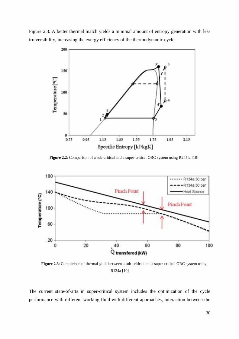
ORC system, due to the higher temperature of the heat input [9]. The enthalpy drop in a super-
critical ORC system is higher which yields a higher amount of useful power, compared to a
sub-critical ORC system with the same turbine inlet temperature, as illustrated in Figure 2.2.
The temperature glide of the super-critical fluid allows a better thermal match with the heat
source temperature within the evaporator, than the fluid below the critical point, as shown in
30
Figure 2.3. A better thermal match yields a minimal amount of entropy generation with less
irreversibility, increasing the exergy efficiency of the thermodynamic cycle.
Figure 2.2: Comparison of a sub-critical and a super-critical ORC system using R245fa [10]
Figure 2.3: Comparison of thermal-glide between a sub-critical and a super-critical ORC system using
R134a [10]
The current state-of-arts in super-critical system includes the optimization of the cycle
performance with different working fluid with different approaches, interaction between the

31
fluid properties and cycle performance, different applications of super-critical cycle, and the
application of zeotropic mixtures [11]. However, the application of super-critical cycle is still
limited as some organic working fluid tend to decompose at high temperature [6]. R245fa might
decompose over 250˚C and produce hydrofluoric acid and carbonyl halides [6]. The high
pressure specification for super-critical ORC requires high pressure-resistant materials for the
piping construction and advanced sealing techniques to avoid the leakage of refrigerants into
the atmosphere.

32
2.2 Selection of Working Fluid for ORC
Selection of suitable working fluid would determine the maximum achievable cycle
efficiency and installed cost of the ORC system. A suitable working fluid has to be determined
in a preliminary cycle design phase to provide an estimation in system’s cost and system
performance to the site owner. The thermodynamic properties of the organic working fluid are
briefly discussed, and the corresponding effects on the ORC system are presented.
Type of working fluid based on saturation vapour curve
The organic working fluids are categorized by the gradient of the saturation curve in a
temperature-entropy (T-s) diagram [12], as shown in Figure 2.4. There are three types of
working fluid, namely wet fluid, dry fluid and isentropic fluid. Wet fluid is characterized with
a negative gradient in a T-s diagram, such as water and ammonia. A minimum amount of
superheat is required at the turbine inlet to avoid the formation of droplets during the expansion
process within the expansion machines. The droplets would impinge on the surface of the
rotating parts of a positive displacement machines or blade surface of a turbine, causing the
cavitation effects and surface damage. An excessively high degree of superheat would,
however, reduce the overall cycle efficiency. Compromise is required to maintain the cycle
efficiency within an acceptable range without sacrificing the life cycle of the turbine. A
common practise in steam plant application is to maintain the minimum dryness fraction above
85% without having an excessive amount of superheat at the turbine inlet [13]. The application
of the wet fluid requires frequent maintenance and overhaul of the turbines.
Dry fluid and wet fluid are better candidates for ORC application without the concern
of condensation along the expansion process. Dry fluid is characterized by the positive gradient
in the T-s diagram. Superheat is not recommended when dry fluid is used as the overall cycle
efficiency would be reduced [14]. If superheat is applied in dry fluid at the turbine inlet, there
would be a larger amount of superheat at the turbine outlet. A larger heating load is required to
apply the superheat and a larger amount of cooling load is required to cool the working fluid
to sub-cooled state, hence reducing the thermal efficiency of the overall cycle. An isentropic
fluid is defined with the close-to-vertical line type of gradient in the T-s diagram such as R245fa
[6]. Isentropic fluid allows the expansion process along the vertical lines in the T-s diagram,
without any condensation. The isentropic fluid is superior compared to the dry fluid as the ORC
working fluid since the isentropic fluid is not excessively superheated at the turbine outlet, in

33
which the cooling load requirement of the condenser is lesser compared to the application of
dry fluid.
Figure 2.4: Temperature-entropy (T-s) diagram of working fluid [15]
Boiling point, freezing point and critical point
The thermodynamics properties of the selected fluid were found to have certain type of
correlations with the thermal efficiency of the ORC. The impact of the boiling temperature of
the working fluid was studied numerically by Mago [16] using different dry fluid, such as
R113, R123, R245ca and iso-butane. The study reveals that the optimal performance of the
ORC system was achieved by the fluid with highest boiling point. The result does not agree
with the study by Aljundi, which demonstrates that the optimal working fluid is not necessary
the working fluid with the highest boiling point [17]. However, a numerical study by Saleh has
validated the hypothesis that the fluid from the same family with the highest boiling point
contribute to the highest ORC thermal efficiency [18]. The correlation between the critical
temperature of the working fluid, expansion ratio across the turbine, and the condensing
temperature has been discussed [13]. A study by Bruno [19] shows that the working fluid with
higher critical temperature result in higher thermal efficiency. The finding is supported by a
study by Wang, in which the ORC system efficiency decreases when the working fluid with
smaller critical temperature were applied in waste heat recovery application [20]. The freezing
point of the fluid does not have direct correlation with the ORC performance. The freezing

34
point of the selected fluid has to be lower than the cycle lowest operating temperature to avoid
choking the condenser.
Compatibility and stability
Organic working fluids usually undergo deterioration and decomposition when the
temperature is much higher than the critical point. Hence, the application in super-critical
region with very high operating temperature has to be taken care of [12]. Organic working fluid
usually exhibits different types of non-favourable properties, such as high flammability in n-
Pentane and toxicity in ammonia. An ideal fluid would be non-corrosive, non-toxic, non-
flammable, non-fouling and compatible with the plant design and plant material. ASHRAE
refrigerant safety classification can be used to indicate the safety level of the fluid [6].
Environmental impact
The main parameters for the consideration of the environmental effects are ozone
depletion potential (ODP), global warming potential (GWP), atmospheric lifetime (ALT),
flammability (F) and toxicity (C). Some of the working fluid have been phased out by Montreal
Protocol such as R-11, R-12, R-113, R-114, R-115 and others will potentially be phased out at
2020 and 2030 such as R-21, R-22, R-123, R-124, R141b [6]. The fluid in consideration for
the ORC system should exclude the soon-to-be-phased-out fluid.
Molecular weight
The molecular weight of the working fluid shows a direct correlation with the turbine
efficiency. Harinck et al. reported that the organic working fluid with higher molecular weight
is preferable for better turbine efficiency [21]. A study by Stijepovic et al. [22] shows that the
increase in molecular weight increases the size parameter, thus increasing the turbine
efficiency, based on equation (2.1). The size parameter, SP, was first derived mathematically
by Macchi [23] using the correlation of specific speed and specific diameter, which was further
simplified by Stijepovic as a function of molar mass, F, molecular weight, M, density at the
turbine exit, ρ, and isentropic drop across the turbine stage at the given pressure ratio, Δhis.
0.25
is
F MSP
h
(13.1)
Though the molecular weight has a positive effect on the turbine performance, evaporator and
condenser with higher heat transfer area are required to compensate the increase in the specific

35
volume of the fluid in vapour form [13]. The effect of the molecular weight on the other turbine
performance index such as work output and pressure ratio has not been investigated.
Latent heat, density and specific heat
High vaporization latent heat, high density and low specific heat are favourable for the
ORC performance and turbine design. High vaporization latent heat allows most of the heat
transfer within the evaporator and minimizes the need of super-heating [24]. Low liquid
specific heat allows the minimal pump power requirement [25]. A study by Bao, however,
shows that there is no direct correlation between the specific work of the liquid and the pump
power requirement [13]. High density fluid is favourable to allow the installation of smaller
size of turbines and heat exchangers units as evaporator and condensers for the similar power
output.
Quantitative Screening Parameters for the Working Fluid
This quantitative method is proposed by Kuo [12] to evaluate the optimal fluid for the
ORC system from the standpoint of the cycle performance. Two parameters have been
proposed, namely Jacob number and Figure of Merit. Jacob number serves as a screening
indicator for different working fluid while figure of merit can be used for screening of the same
fluid under different operating conditions. Kuo et al. [12] found that lower Jacob number and
figure of merit result in higher system thermal efficiency. Jacob number is defined as the ratio
of sensible heat transfer and latent heat of evaporation.
p
fg
C TJa
h
(13.2)
0.8
0.1 cond
evap
TFOM Ja
T (13.3)
Where Cp is specific heat at constant pressure, hfg is latent heat of evaporation, FOM is figure
of merit, Ja is Jacob number, Tevap is evaporating temperature, Tcond is condensing temperature,
and ΔT is the difference of evaporating temperature and condensing temperature of the
thermodynamic cycle.

36
Summary of Proposed Working Fluid for ORC based on Current State-of-Art
Selection of optimal working fluid for the ORC system using different objective
functions, such as cycle performance, exergy efficiency, and heat-exchange areas, has been
performed extensively for the past decades, in both numerical simulation and experimental
validations. Different types of application have different optimal working fluid. Research in
working fluid selection with corresponding field application is compiled in Table 2.1. Among
the working fluids, the most recommended fluid for ORC is R245fa, followed by R236ea
and benzene for sub-critical ORC system.

37
Table 2.1: Recommended fluid from the past research with different screening criteria
Authors Application Cycle Cond.
Temp (0C)
Evap. Temp
(0C) Considered Fluid
Recommended fluid (Efficiency / Net
Power Output/cost per kWh)
Guo et al. (2011) [9, 26] Geothermal
subcritical
ORC 35 90 * 27 fluid R236ea, E170, R600, R141b
trans-
critical 25 80 - 120 *
Natural and conventional fluid
R125, R32, R143a
trans-
critical 25 >100 * R218, R143a, R32
Wang et al. (2011) [27] Waste Heat
Recovery
Sub-
critical 27 - 87 0.2 - 2 Mpa
R245fa, R245ca, R236ea, R141b,
R123, R114, R113, R11, Butane
R245fa, R245ca (environmental
friendly) and R113, R123, R11, R141b
(high performance)
Vankeirsbilck et al. (2011)
[4]
Waste Heat
Recovery
Sub-
critical 40 120-350*
R245fa, Toluene, (cyclo)-pentane,
Solkatherm, 2 silicone oils (MM and
MDM), OMTS, HDMS
Toluene, OMTS, HMDS, cyclo-pentane
Rayegan and Tao (2011)
[28] Solar
Sub-
critical 25
130 Refrigerants and non-refrigerants
(117 fluid)
refrigerant (R245fa, R245ca), non-
refrigerant (Acetone, Benzene)
85 refrigerant (R245fa, R245ca, E134),
non-refrigerant (Cyclohexane, Benzene)
Kuo, Hsu, Cliohang, Wang
(2011) [12]
Not specified
(50kW)
Sub-
critical 45 108
R123, R236fa, R245fa, R600, n-
Pentane
R123 followed by n-Pentane, R245fa,
R600, R236fa
Aljundi (2011) n/a n/a 30 50-140
RC-138,R227ea, R113, isobutane,
n-butane, n-hexane, isopentane, neo-
pentane, R245fa, R236ea, C5F12,
R235fa
n-hexane
Papadopoulos et al. (2010)
[25] n/a
Sub-
critical n/a n/a
Hydrocarbons, Hydrofluorocarbons,
conventional fluid R611
Mikielewicz and
Mikielewicz (2010) CHP n/a 50 170
R365mfc, Heptane, Pentane, R12,
R141b, Ethanol Ethanol

38
Fankam et al. (2009) Solar Sub-
critical 35 60 - 100 Refrigerants R125a, R600, R290
Tchanche et al. (2009) Solar n/a 35 60-100 Refrigeratns R152a, R600, R290
Facao (2009) Solar n/a 45 120 / 230
Water, n-Pentane, HFE7100,
Cyclohexane, Toluene, R245fa, n-
dodecane, iso-butane
n-dodecane
Dai (2009) [29] Waste heat
recovery n/a 25 145*
Water, ammonia, butane, isobutane,
R11, R123, R141b, R236ea,
R245ca, R113
R236ea
Desai (2009) [30] Waste heat
recovery n/a 40 120
Alcanes, Benzene, R113, R123,
R141b, R236ea, R245ca, R245fa,
R365mfc, Toluene
Toluene, Benzene
Gu (2009) Waste heat
recovery n/a 50 80-220 R600a, R245fa, R123, R113 R113 and R123
Saleh et al. (2007) Geothermal Sub-
critical 30 100
Alkanes, fluorinated alkanes, ethers
and fluorinated ethers
RE134, RE245, R600, R245fa, R245ca,
R601
Drescher and Bruggemann
(2007) Biosmass CHP n/a 90* 250 - 350 *
ButylBenzene, Propylbenzene,
Ethylbenzene, Toluene, OMTS Alkyl Benzenes
Hettiarachchia et al. (2007)
[3] geothermal
Sub-
critical 30* 70-90 Ammonia, n-Pentane, R123, PF5050 Ammonia
Lemort et al. (2007) Waste Heat
Recovery
Sub-
critical 35 60-100 R245fa, R123, R134a, n-Pentane R123, n-Pentane
Borsukiewicz-Gozdur and
Nowak (2007) Geothermal
Sub-
critical 25 80-115
propylene, R227ea, RC318, R236fa,
ibutane, R245fa Propylene, R227ea, R245fa
El Chammas and Clodic
(2005)
Waste Heat
Recovery
(Internal
Combustion
Engine)
n/a 55 (100 for
water)
60 - 150
(150 - 260
for water)
Water, R123, isopentane, R245ca,
R245fa, butane, isobutene, R152a Water, R245ca and Iso-pentane
Maizza and Maizza [24] n/a Sub-
critical 35-60 80-110 Unconventional working fluid R123, R124
* indicate temp of heat source/heat sink **the table is extended from [31] and [32]

39
2.3 Industrial ORC Technology: A brief summary
ORMAT has commercialized the ORC system and manufactured small power units in
Massachusetts in early 1970 [33]. The company has ventured into geothermal application,
installing the first ORMAT Energy Convertor (OEC) in Wabuska facility outside of Yerington,,
Nevada in 1984. ORMAT has then expanded the business worldwide with over 626 MW
geothermal plants, and over 1,750 MW of installed OEC capacity in year 2014 [33]. Turboden
is another leading company in development and production of ORC technology, based in Italy
and founded by Mario Gaia, Professor of Energy at the Politecnico di Milano [34]. Turboden
manufactures ORC units from 300 kW for combined heat and power (CHP) application in early
1980 [35]. Turboden has expanded the business and developed the off-the-shelf ORC units
between 300 kW and 10 MW [34]. Both ORMAT and Turboden are the pioneers of the
commercial ORC products with their extensive experiences in the field over decades. Figure
1.6 shows the number of the ORC sites and the power distributions of the ORC sites installed
by a number of ORC companies. ORMAT has the largest installed capacities whereas Turboden
has the most number of sites in the market. The figure also shows a number of ORC
manufacturers, including Tri-O-Gen, UTC Power, BNI, Electratherm, and etc. A market
analysis on the commercial ORC technologies was performed and the current ORC
manufacturers and suppliers with their corresponding technologies were presented in Table 2.2.
(a)
44%
24%
22%
3%2%
1%2%
1% 1% 0%
0%
Number of ORC sites installed by vendors
Turboden
Ormat
Maxxtec / Adoratec
GMK
Tri-O-Gen
UTC Power
BNI
Eletractherm
Enex / Geysir
Cryostar
Calnetix

40
(b)
Figure 2.5: (a) The sites installed and b) the total power distributions by the major ORC manufacturers [36]
9%
86%
3% 2%
Power distributions of the ORC sites installed
Turboden
Ormat
Maxxtec / Adoratec
Others

41
Table 2.2: Summary of some ORC manufacturers with the corresponding technology and products
Suppliers Types of Heat
Source
Heat Source
Temp. Heat Carrier
Thermal
Input (kW) Power Output Units Technology
Ormat
Geothermal
Low - High Geothermal fluid/steam n/a
250 kW to 20 MW
OEC (Custom-made) Fluid: n-pentane Heat Recovery (200 kWe to 72
MWe)
Solar
Turboden
(UTC)
Biomass
in300/out240 Thermal Oil 3340 to
12020
643 kW to 2304
Kw TD6CHP - TD22CHP n/a
in310/out210 Thermal Oil 4155 to
13075 1 MW to 3 MW
TURBODEN 12 HRS &
TURBODEN 24 HRS n/a
Heat Recovery
240 - 310 Exhaust gas, refineries
hot streams, jacket
cooling water of engines,
condensing organic fluid
2.5 MW to
50 MW 600 Kw to 10 MW
TURBODEN 6/7HR -
TURBODEN 50 to 100
HR
Fluid: OMTS,
Solkatherm
Axial Turbines
in310/out210 4155 to
13075 1 MW to 3 MW
TURBODEN 12 HRS &
TURBODEN 32 HRS n/a
Geothermal Min 91 degree C Hot water/steam n/a 280 kW PureCycle® power system n/a
1.5 MW n/a n/a
Infinity
Turbine ® Heat Recovery
Below 100
degree C (>80
degree C)
Compressed air, steam,
water, etc. n/a
5kW-10kW,
50,250 kW
IT50, IT10, IT250, Itmine
or Itxr
Fluid: R134a
Radial Turboexpander
GE Energy Heat Recovery in143/out127
Pressurized Hot
Water,saturated steam,
gas
980 kW 125 kW Clean Cycle™ 125
Maxxtec /
Adoratec Biomass 320/245 Thermal Oil
1650 kW to
12970 kW
300 kW to 2400
kW
AD300 TF-plus -
AD2400TF-plus Fluid : OMTS
GMK Heat Recovery 300 degree C Thermal Oil 3.5 - 10.0
MW 0.5 - 5.0 MW INDUCAL®
3000 rpm multi-stage
axial turbines (KKK)

42
Fluid: GL160 (GMK
patented)
Biomass 350 degree C Thermal Oil 3.5 - 10.0
MW 0.5 - 2.0 MW ECOCAL® n/a
Geothermal 100 °C up to
250 °C Thermal waters
3.5 - 125.0
MW 0.5 - 15.0 MW GEOCAL® n/a
TRI-O-GEN Heat Recovery > 350 degree C Toluene (direct exposed
to heat source)
450 - 900
kWth 60 - 165 kWe Tri-O-Gen ORC Turbo Expander
Calnetix
Technologies Heat Recovery n/a n/a n/a 125 kW
Thermapower™ Organic
Rankine Cycle (ORC)
Modules
n/a
ElectraTherm
Heat Recovery
88 °C -116°C
Other Liquid Waste Heat
Sources
n/a 18 - 65 kWe Series 4000 Green
Machine Twin Screw Expander Solar Hot Water Heat Source
Biomass Thermal Oils
Geothermal Hot Water Heat Source
Cryostar Geothermal 100 – 400 °C n/a n/a 1.5 MW (France)/
3.3MW (Germany) n/a
Radial Inflow Turbine
Fluid: R245fa, R134a
koehler-ziegler Waste Heat 90 – 200 °C n/a n/a 50 – 200 kWe n/a
Fluid: Hydrocarbons
Steam Turbine (screw
expander)
Free Power Waste Heat 180 – 225 °C n/a n/a n/a FP85, FP 100, FP 120 n/a
Note: The table is compiled from [31] and further extended from the official website from the relevant companies
43
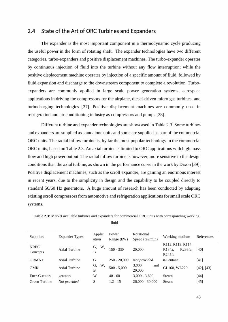
2.4 State of the Art of ORC Turbines and Expanders
The expander is the most important component in a thermodynamic cycle producing
the useful power in the form of rotating shaft. The expander technologies have two different
categories, turbo-expanders and positive displacement machines. The turbo-expander operates
by continuous injection of fluid into the turbine without any flow interruption; while the
positive displacement machine operates by injection of a specific amount of fluid, followed by
fluid expansion and discharge to the downstream component to complete a revolution. Turbo-
expanders are commonly applied in large scale power generation systems, aerospace
applications in driving the compressors for the airplane, diesel-driven micro gas turbines, and
turbocharging technologies [37]. Positive displacement machines are commonly used in
refrigeration and air conditioning industry as compressors and pumps [38].
Different turbine and expander technologies are showcased in Table 2.3. Some turbines
and expanders are supplied as standalone units and some are supplied as part of the commercial
ORC units. The radial inflow turbine is, by far the most popular technology in the commercial
ORC units, based on Table 2.3. An axial turbine is limited to ORC applications with high mass
flow and high power output. The radial inflow turbine is however, more sensitive to the design
conditions than the axial turbine, as shown in the performance curve in the work by Dixon [39].
Positive displacement machines, such as the scroll expander, are gaining an enormous interest
in recent years, due to the simplicity in design and the capability to be coupled directly to
standard 50/60 Hz generators. A huge amount of research has been conducted by adapting
existing scroll compressors from automotive and refrigeration applications for small scale ORC
systems.
Table 2.3: Market available turbines and expanders for commercial ORC units with corresponding working
fluid
Suppliers Expander Types Applic
ation
Power
Range (kW)
Rotational
Speed (rev/min) Working medium References
NREC
Concepts Axial Turbine
G, W,
B 150 - 330 20,000
R112, R113, R114,
R134a, R236fa,
R245fa
[40]
ORMAT Axial Turbine G 250 - 20,000 Not provided n-Pentane [41]
GMK Axial Turbine G, W,
B 500 - 5,000
3,000 and
20,000 GL160, WL220 [42], [43]
Ener-G-rotors gerotors W 40 - 60 3,000 - 3,600 Steam [44]
Green Turbine Not provided S 1.2 - 15 26,000 - 30,000 Steam [45]

44
COGEN
Microsystems Piston expander
W,
CHP < 20 Not provided Not provided [46]
Infinity Turbine Radial inflow
turbine G, W 10 - 250 3,600 R245fa, R134a [47]
Verdicorp Radial inflow
turbine W 20 - 115 Up to 45,000 R245fa [48]
Tri-O-Gen Radial inflow
turbine W, B 60 - 165 25,000 Toluene [43], [49]
GE Energy Radial inflow
turbine W 125 26,500 R245fa [43], [50]
Zuccato-
Energia
Radial inflow
turbine W 50, 150 15,000 R245fa [51]
Cryostar Radial inflow
turbine
W,
CHP 500 - 15,000 6,000 - 33,000 Not provided [52]
Atlas Copco
Radial inflow
turbine/ Axial
Turbine
G, W 200 - 25,000 14,000* Isobutane * [53]
Turboden
Radial inflow
turbine/ Axial
Turbine
G, W,
B, CHP 200 - 15,000 Not provided R134a, Steam [34], [54]
Exergy Radial outflow
turbine
G, W,
B 400 - 5,500 3,000 Steam [55]
Exa-Energie Screw expander W,
CHP 15 - 150 3,000 - 3,600
R245fa, R134a,
Toluene [56]
Electra-Therm Screw expander W,
CHP, B 35 - 110 3,000 - 3,600 R245fa [43]
Air Squared Scroll expander W 1 - 10 3,000 - 3,600 R245fa [52]
ENEFTECH Scroll expander W,
CHP 5 - 30 3,000 R245fa [57]
Icenova
Engineering Scroll expander W 15, 30 3,000 - 3,600 R245fa [56]
The design and development of expansion machines for ORC system involves a number
of research in different fields, including modelling improvement in the cycle preliminary design
phase, application of more accurate equations of state (EoS) to model the real gas effects,
advanced improvement in design and analysis of axial and radial turbines, and evaluation of
the feasibility of different positive displacement machines, such as scroll expander, screw
expander, vane expander, and piston expander. An ORC system has to be modelled to
determine the optimal cycle configuration and working fluid for the best cycle performance
before conducting a detailed design analysis on the system components. A number of
assumptions is usually made to reduce the computational efforts, including the constant
efficiency of pump and turbine. One of the disadvantages of assuming the constant efficiency
of the pump and the turbine is the system performance and the turbine performance cannot be

45
represented precisely at different operating condition. The turbine performance is very sensitive
to the type of machines and the operating condition. Radial inflow turbine is more sensitive to
the design point compared to axial turbine, in which the representation of the off-design
performance of the radial inflow turbine would be deviated significantly from the actual
condition if the performance is assumed constant [39]. Different turbine modelling approaches
have been incorporated into the cycle preliminary design phase to improve the accuracy of the
cycle model, as the following:
the isentropic efficiency of the turbine has been modelled as a function of volumetric
flow rate of the working fluid and enthalpy drop across the turbine [58],
the isentropic efficiency has been modelled as a function of specific speed, volumetric
expansion ratio, and the size parameter [59], and
the turbine design and meanline analysis program has been coupled to the cycle
design [60-62]
One of the innovations in current ORC technology is the application of scroll machines
as the expanders to generate electricity in the range of a few kilowatts to thirty kilowatts. An
initiative has been taken by a few researchers to convert the scroll compressors from
automobile application and from refrigeration system into scroll expanders [63-67]. The
conversion of the scroll compressors into scroll expanders is feasible with an acceptable range
of isentropic efficiency for the expanders. Different types of industrial scroll compressors have
been investigated and converted into expansion machines for ORC, with the maximum
efficiency between 70 and 80% for hermetic refrigeration scroll compressors [68-71], 60 and
70% for open-drive automotive scroll compressors [72-74], 70 and 78% for scroll air
compressors [66, 75, 76], and 80% for semi-hermetic automotive compressor [77]. Three
different modelling techniques have been developed to study the steady state performance and
the dynamic behaviour of the scroll expander, namely deterministic model, semi-empirical
model, and empirical model. Deterministic model is the full mathematical model describing
the dynamic motion of the scroll expander for the full revolution, coupled to the conservation
of mass flow, leakage model, suction pressure and discharge pressure loss [78-80], and the heat
transfer between the fluid, casing, and the atmosphere. The deterministic model is able to
provide the information of the variation of mass flow with the rotation angle, under-expansion
or over-expansion, and shaft power as a function of the shaft speed without conducting an
experiment. Empirical model has been developed to correlate the operating parameters to the

46
performance parameters. Fundamental thermodynamics behaviour is, in most cases, ignored in
the empirical model. Semi-empirical model has been developed by taking into account of the
mass balance, pressure drop, expansion process, and heat balance of the scroll system. Eight
model parameters were identified and the values were determined from the experimental
measurements [66]. The semi-empirical model was then applied to investigate the mass flow
and shaft power at different pressure ratio with maximum deviation of less than 5% [66]. One
of the interesting experimental works for scroll expanders is the investigation of the breakdown
of losses of a scroll expander [69]. The study shows that both the mechanical loss and the motor
loss contribute to the low isentropic efficiency of the scroll expander, even at the optimal
operating condition. Other than the adaptation of scroll compressors as scroll expanders, a
design procedure, known as 8-dimensional planar curve framework, was adapted for the
geometrical design of scroll expanders [81]. The method was demonstrated by designing a
scroll geometry for a 3 kWe ORC system with maximum isentropic efficiency of 85% [81].
There are different positive displacement machines suitable for the application in an
ORC system. Among the machines, screw expander is another popular technology with low
flow and low power output less than 250 kWe. Screw expander is comprised of either a helical
rotor or a pair of helical rotors with a casing. The volume between the rotors and the casing
changes as a function of the rotational angle. The power is transferred from the expansion of
the fluid to the rotor shafts by the pressure difference on the rotors, which changes with the
fluid volume during the rotation [82].The technology of screw machine has been studied
extensively by Smith [83-92] over 20 years in different applications with different modelling
techniques, including thermodynamic analysis [84], full flow field study using computational
fluid dynamics (CFD) [83] and fluid-solid interactions [93]. The main suppliers for screw
machines for ORC application include Electratherm (twin screw expander), BEP Europe
(mono screw machine), and Opcon (Lysholm expanders) [94]. The current research study of
screw expander includes the development of an empirical-based model for expander’s
performance [95], experimental study of an ORC system using screw expander [96],
preliminary testing of a screw expander by using a compressed air test rig [97], and evaluation
of the performance of the screw expander was evaluated with different intake pressure [98] and
different clearance between the rotors and the casing [99]. The screw expander technology has
been evaluated using three-dimensional CFD model to study the performance of different
designs under different pressure ratio [100] and evaluate the development of pressure
distribution using single phase flow and two phase flow [101].

47
Ge-rotor, piston expander, and rotary vane expander are less popular than the scroll
expander. A scroll expander and a ge-rotor were tested using R123 [70] at 3 kWe and 2 kWe
with isentropic efficiency of 83% and 85%, respectively. A small ge-rotor with built-in volume
ratio of 2 was tested with nominal power of 10 We with an isentropic efficiency of 11% [102].
The low isentropic efficiency is attributed to the large frictional force at small power, which
could be improved for an optimal ORC unit. Ener-G-Rotors produces ge-rotors as commercial
ORC expander units with nominal power of 40 and 60 kWe. Piston expander and rotary vane
expander are potential ORC expansion machines with low isentropic efficiency [13]. A number
of drawbacks in utilizing the piston expander as expansion machines were stated [13],
including lubrication issues and poor breathing characteristics attributed to the high frictional
losses across the valves. Two research prototype units of piston expander were tested using
carbon dioxide as the working medium, with isentropic efficiency of 11% [103] and 62% [104].
A rotary vane expander (adapted from an air motor) was tested [105] using HFE7000 with a
measured power of 860.7We and approximately 55% isentropic efficiency. A number of
prototype research of the piston expander and vane expander was presented in Table 2.4. The
application of these machines in the ORC application is limited due to the low isentropic
efficiency of the piston expander and vane expander, attributed to the poor sealing, high
leakage flow, and high frictional losses between the contacting surfaces. A high isentropic
efficiency is usually favourable commercially to increase the energy return on investment
(EROI), which further impedes the research development of these machines.
Table 2.4: The prototype research of reciprocating piston expander and rotary vane expander [13]
Researchers Type of machines Working
fluid
Max. Isentropic
efficiency (%)
Power
(kW)
Pressure
ratio
Baek et al. [106] Reciprocating piston
expander CO2 10.5 24 2.1
Zhang et al. [107] Reciprocating piston
expander CO2 62 - 2.4
Mohd et al. [108] Rotary vane expander R245fa 48 0.03 24
Yang et al. [109] Rotary vane expander CO2 23 - -
Qiu et al. [105] Rotary vane expander HFE7000 55 1.7 2.1
The radial inflow turbine is the most popular solution for the ORC application, from a
few kWe to a few MWe. An ORC expansion machine has to be able to handle the expansion
of dense gas at high pressure ratio, with low flow rate and low enthalpy drop. A single stage

48
radial inflow turbine is more superior than a single stage axial turbine for the following reasons
[110]:
A radial inflow turbine can be optimized for different geothermal resources through
minor changes.
High turbine efficiency can be achieved for part-load condition using variable inlet
guide vanes.
The turbine blade profile is less sensitive to the deviation from manufacturing,
compared to axial turbine.
The blade structure is more robust under high blade loading with high density fluid.
Radial inflow turbine shows a better rotor-dynamic stability and higher stiffness.
Different researches have been conducted extensively on the radial inflow turbine, prior to the
development of the ORC technology, mainly in turbocharging and gas turbine sectors. The
conventional design and development process of a radial inflow turbine is very intricate, and
one of the design approaches has been proposed by Baines, as illustrated in Figure 2.6 [111].
The preliminary design stage uses the least computational effort with the highest efficiency
improvement for the turbine design. The preliminary design process aims to provide the overall
geometry of the turbine by calculating the velocity vector at the turbine inlet and the exit, and
solve the law of conservation of mass, energy, and momentum to determine the mass flow rate
and the thermodynamic conditions at each stations. A number of preliminary design approaches
using meanline analysis has been developed about half a century ago [112-114]. The
preliminary design approaches have been coupled to different optimization methods to provide
the best geometry based on the weighted specifications as outlined by the designers. One of the
evolutionary algorithms, known as Genetic Algorithm (GA), is commonly applied by a number
of researchers [115-119]. Other optimization techniques have been coupled to the preliminary
design phase, such as particle swarm optimization [120], multi-objective optimization [61],
and DIRECT algorithm [60]. The preliminary design of radial turbine has been commonly
implemented using the perfect gas assumption to reduce the computational effort but the
thermodynamic properties of hydrocarbons or refrigerants in an ORC system do not agree well
with the ideal gas law [21]. Hence, the fluid database has often been coupled to the preliminary
design program to improve the accuracy of the turbine design model [121, 122]. Aerodynamic
study on the turbine blade profile gains increased attention, especially for the ORC turbine due
to the use of dense gas, with behaviour deviated significantly from the ideal gas law.
Aerodynamic analysis was performed across the ORC turbine to investigate the unsteady

49
interaction between nozzle vanes and rotor blade for transonic flow [123] and the detailed
analysis of shock wave patterns evolution within the blade passage [124]. Aerodynamic study
was also conducted to model the supersonic flow within the blade passage of the nozzle vanes
[125-127] to improve the nozzle design. One of the concerns of the ORC turbine is the turbine
performance in different operating conditions, as the pressure ratio and mass flow rate of the
ORC would fluctuate as a function of ambient temperature for a air-cooled geothermal binary
plant [128]. The radial inflow turbine is very sensitive to the operating condition, compared to
axial turbine [39]. The performance gain of the application of variable inlet guide vanes in an
ORC turbine was investigated numerically [53] and experimentally [129] in a geothermal
binary plant for a wide range of operating conditions.
Figure 2.6: The design approach of turbine [111]
Radial outflow turbine is another innovative solution proposed and installed by
EXERGY for geothermal, biomass and waste heat recovery application [130]. The gas flow is
directed into the smaller wheel side and out from the turbine at the larger wheel side. The radial
outflow turbine was reported to spin at low speed, with a large pressure ratio across multiple
stages on a single disk. However, the radial outflow turbine tends to demonstrate a lower
specific work output compared to an axial turbine and a radial inflow turbine with similar size
[111]. An in-house design program for radial outflow turbine, known as zTurbo incorporating

50
the meanline analysis and optimization approach has been developed [131, 132]. The pressure
field of the design outcome has been analysed and validated using an in-house through-flow
solver, TzFlow [132]. The complex flow field in the radial outflow turbine was studied using
ANSYS-CFX and the interaction between compressible flow effects on the blade profile design
has been presented [133].
Axial turbine is a turbomachine for high flow rate and high pressure ratio. The axial
turbine technology was developed over half a century ago in military and aerospace
applications, which was then extended into the power generation application as steam turbine
and gas turbine. Different empirical losses models were developed and validated for air and
steam applications, including Ainley-Mathieson model [134], Craig-Cox model [135], Kacker-
Okapuu model [136], and etc. The comparison between different empirical loss models for the
ORC application [137] shows some discrepancies in the performance evaluation. A concept
and design of an ORC cascade wind tunnel was proposed [138] with the aim to develop loss
correlations of different aerofoil profile for ORC application. A commercial turbine design
package, AxStream, incorporating the conventional design approach with real fluid database,
was used to design a single stage axial turbine for R245fa with rated power of 250 kWe and
estimated isentropic efficiency over 80% [139]. The axial flow configuration also allows the
use of the multiple stage of axial turbines for high expansion ratio (up to 20:1 with a 4-stage
configuration) with high isentropic efficiency [40]. Axial turbine, however, is not suitable for
small system with low volumetric flow rate. A full admission axial turbine was designed for n-
Pentane with rated power of 2 kWe [140]. The isentropic efficiency was found at 57% at the
design point as compromise was required for a feasible design. A partial admission turbine was
designed and tested for low flow application with measured isentropic efficiency of 53% [141].
The application of accurate gas model to predict the thermodynamic properties of the
selected fluid is crucial in both turbine design and performance analysis. The adaptation of
perfect gas model would yield large deviations up to 25% in density, sonic velocity, and total
pressure loss, and 10% in Mach number, pressure and temperature distribution [142]. Another
study by Lujan [143] shows that the maximum relative deviations using ideal gas equation are
over 100% for pressure and heat capacity at constant volume, less than 70% for local speed of
sound and heat capacity at constant pressure, and 50% for internal energy and enthalpy of the
fluid. Though the deviation in the estimation of thermodynamic properties is significant, the
distribution of thermodynamic properties in the flow field using ideal gas equation is similar
to the flow field using real gas model [144]. A numerical study by Michele et al. [124] reports

51
that the use of perfect gas is not able to capture the working fluid behaviour across the whole
expansion process accurately, but the behaviour within a single component (such as nozzle or
rotor) was predicted successfully. A number of non-dimensional parameters deduced from
similarity criterion was compared for a turbine using two different fluid, namely R245fa and
air [145]. A large deviation in the non-dimensional parameters was found, and the error was
attributed to the influence of the specific heat ratio [145]. The summary of the review of the
current state-of-art of ORC expansion machine was illustrated by a fish bone diagram in Figure
2.7.
The current researches on the ORC turbine can generally be divided into two main
categories: the adaptation of the positive displacement machines for the ORC application, and
the improved numerical model to optimize the current turbine design and analysis in terms of
steady and unsteady flow. The adaptation of the turbine from one working fluid into another is
yet to be investigated or studied. Hence, the main contribution of this thesis is to fill in this
engineering gap by presenting the SMC-DTR approach to design and optimize the ORC system
to the resource condition by adapting the off-the-shelf turbines.

52
Figure 2.7: Current state-of-art of ORC expansion machines
ORC Similarity Concept Gas Model Other machines
Axial Radial Screw Expander Scroll Expander
Deviations in
thermodynamics
using different EoS
Deviations in ideal
gas model and real
gas model
Deviations in flow
physics and blade
loading
Optimization using GA
in preliminary design
Radial outflow
(preliminary, in-
house-code, CFD
of nozzle)
FEA (thermal
load, global stress)
Unsteadiness due
to shock from
nozzle TE
CFD (flow physics,
losses due to dense gas,
through flow analysis,
distribution of force and
entropy gain in rotor)
Supersonic
flow in nozzle
Preliminary
design
Couple to
turbine loss
model
Optimization
Working fluid
selection
Analytical &
Empirical model
CFD model of
fluid expansion
Experimental
validation
Conversion from
compressor
Geometrical
optimization
Analytical, empirical/
semi-empirical model
Experimental
evaluation
Conventional
design process
Partial admission
for very small flow
rate (modelling &
experiment)
Compare diff.
losses models
if real gas is
used
Justify the
importance of
specific heat
Performance
prediction and
aerodynamic
loading for single
components
Validation
against one
channel CFD
model
Selection chart
(screw & scroll)
Conversion of
air motor
Conversion of
vane expander
Feasibility of
piston expander
Retrofit of
refrigeration system
ORC
Expansio
n Machine
53
2.5 References
1. Agency, I.E. IEA Electricity Information 2012. 2012.
2. Overview of Existing Power Generation Turbine Designs. 2000 - 2014, SoftInWay
Incorporation.
3. Madhawa Hettiarachchi, H.D., et al., Optimum design criteria for an Organic Rankine
cycle using low-temperature geothermal heat sources. Energy, 2007. 32(9): p. 1698-
1706.
4. Vankeirsbilck, I., et al., Organic rankine cycle as efficient alternative to steam cycle for
small scale power generation. Proceedings of 8 th International Conference on Heat
Transfer, Fluid Mechanics and Thermodynamics, Pointe Aux Piments (Mauritius),
2011.
5. Li, J., et al., Energetic and exergetic investigation of an organic Rankine cycle at
different heat source temperatures. Energy, 2012. 38(1): p. 85-95.
6. Chen, H., D.Y. Goswami, and E.K. Stefanakos, A review of thermodynamic cycles and
working fluids for the conversion of low-grade heat. Renewable and Sustainable Energy
Reviews, 2010. 14(9): p. 3059-3067.
7. Zhang, X., M. He, and Y. Zhang, A review of research on the Kalina cycle. Renewable
and Sustainable Energy Reviews, 2012. 16(7): p. 5309-5318.
8. Bombarda, P., C.M. Invernizzi, and C. Pietra, Heat recovery from Diesel engines: A
thermodynamic comparison between Kalina and ORC cycles. Applied Thermal
Engineering, 2010. 30(2–3): p. 212-219.
9. Guo, T., H. Wang, and S. Zhang, Comparative analysis of natural and conventional
working fluids for use in transcritical Rankine cycle using low‐temperature geothermal
source. International Journal of Energy Research, 2011. 35(6): p. 530-544.
10. Karellas, S., A. Schuster, and A.-D. Leontaritis, Influence of supercritical ORC
parameters on plate heat exchanger design. Applied Thermal Engineering, 2012. 33–
34(0): p. 70-76.
11. Radulovic, J. and N.I. Beleno Castaneda, On the potential of zeotropic mixtures in
supercritical ORC powered by geothermal energy source. Energy Conversion and
Management, 2014. 88(0): p. 365-371.
12. Kuo, C.-R., et al., Analysis of a 50kW organic Rankine cycle system. Energy, 2011.
36(10): p. 5877-5885.
13. Bao, J. and L. Zhao, A review of working fluid and expander selections for organic
Rankine cycle. Renewable and Sustainable Energy Reviews, 2013. 24: p. 325-342.
14. Hung, T.C., T.Y. Shai, and S.K. Wang, A review of organic rankine cycles (ORCs) for
the recovery of low-grade waste heat. Energy, 1997. 22(7): p. 661-667.

54
15. Shu, G., et al., Parametric and working fluid analysis of a dual-loop organic Rankine
cycle (DORC) used in engine waste heat recovery. Applied Energy, 2014. 113(0): p.
1188-1198.
16. Mago, P.J., et al., An examination of regenerative organic Rankine cycles using dry
fluids. Applied thermal engineering, 2008. 28(8): p. 998-1007.
17. Aljundi, I.H., Effect of dry hydrocarbons and critical point temperature on the
efficiencies of organic Rankine cycle. Renewable Energy, 2011. 36(4): p. 1196-1202.
18. Saleh, B., et al., Working fluids for low-temperature organic Rankine cycles. Energy,
2007. 32(7): p. 1210-1221.
19. Bruno, J.C., et al., Modelling and optimisation of solar organic rankine cycle engines
for reverse osmosis desalination. Applied Thermal Engineering, 2008. 28(17): p. 2212-
2226.
20. Liu, B.T., K.H. Chien, and C.C. Wang, Effect of working fluids on organic Rankine
cycle for waste heat recovery. Energy, 2004. 29(8): p. 1207-1217.
21. Harinck, J., Super-and Transcritical Fluid Expansions, in Mechanical, Maritime and
Materials Engineering. 2010, Delft University of Technology.
22. Stijepovic, M.Z., et al., On the role of working fluid properties in Organic Rankine
Cycle performance. Applied Thermal Engineering, 2012. 36: p. 406-413.
23. Macchi, E. and A. Perdichizzi, Efficiency prediction for axial-flow turbines operating
with nonconventional fluids. ASME Journal of Engineering for Power, 1981. 103: p.
718e24.
24. Maizza, V. and A. Maizza, Working fluids in non-steady flows for waste energy
recovery systems. Applied Thermal Engineering, 1996. 16(7): p. 579-590.
25. Papadopoulos, A.I., M. Stijepovic, and P. Linke, On the systematic design and selection
of optimal working fluids for Organic Rankine Cycles. Applied Thermal Engineering,
2010. 30(6-7): p. 760-769.
26. Guo, T., H. Wang, and S. Zhang, Fluids and parameters optimization for a novel
cogeneration system driven by low-temperature geothermal sources. Energy, 2011.
27. Wang, E.H., et al., Study of working fluid selection of organic Rankine cycle (ORC) for
engine waste heat recovery. Energy, 2011. 36(5): p. 3406-3418.
28. Rayegan, R. and Y.X. Tao, A procedure to select working fluids for Solar Organic
Rankine Cycles (ORCs). Renewable Energy, 2011. 36(2): p. 659-670.
29. Dai, Y., J. Wang, and L. Gao, Parametric optimization and comparative study of
organic Rankine cycle (ORC) for low grade waste heat recovery. Energy Conversion
and Management, 2009. 50(3): p. 576-582.
30. Desai, N.B. and S. Bandyopadhyay, Process integration of organic Rankine cycle.
Energy, 2009. 34(10): p. 1674-1686.

55
31. Quoilin, S. and V. Lemort. Technological and economical survey of Organic Rankine
Cycle systems. in 5th European Conference Economis and Management of Energy in
Industry. 2009. Algarve, Portugal.
32. Quoilin, S., et al., Thermo-economic optimization of waste heat recovery Organic
Rankine Cycles. Applied Thermal Engineering, 2011. 31(14–15): p. 2885-2893.
33. Nordquist, J., DOE’s Quadrennial Energy Review Stakeholder Meeting
Natural Gas Transmission, Storage & Distribution. 2014: Pittsburgh, PA.
34. [cited 2014 3rd Sept]; Available from: http://www.turboden.eu/en/home/index.php.
35. Bronicki, L. Short review of the long history of ORC power systems. in 2nd
International Seminar on ORC Power Systems (ORC2013), Rotterdam, Oct. 2013.
36. Enertime. Markets and actors in Organic Rankine Cycle. 2009 [cited 2012 15th June];
Available from: http://www.cycle-organique-rankine.com/market-markers.php#2.
37. Meher-Homji, C.B. ‘The Historical Evolution of Turbomachinery. in Proceedings of
the 29th Turbomachinery Symposium, Texas A&M University, Houston, TX. 2000.
38. Hundy, G., A.R. Trott, and T. Welch, Refrigeration and Air-conditioning. 2008:
Butterworth-Heinemann.
39. Dixon, S.L. and C. Hall, Fluid Mechanics and Thermodynamics of Turbomachinery.
2010, Butterworth-Heinemann: Burlington.
40. David Japikse, F.D.B., Maxwell Hurgin, Keith Patch. Development of a 300 kWe
Integrated Axial Turbine and Generator for ORC Applications. in 2nd Internal Seminar
on ORC Power Systems: Turbo Expanders II. 2013. De Doelen, Rotterdam, The
Netherlands: American Society of Mechanical Engineers (ASME).
41. Nasir, P., et al., Utilization of Turbine Waste Heat to Generate Electric Power at
Neptune Plant. 2004.
42. GMK. [cited 2014 22nd Sept]; Available from: http://www.gmk.info/.
43. Quoilin, S., et al., Techno-economic survey of Organic Rankine Cycle (ORC) systems.
Renewable and Sustainable Energy Reviews, 2013. 22(0): p. 168-186.
44. Newell, M. [cited 2004 29th Aug]; Available from: http://www.ener-g-rotors.com/.
45. Green Turbine, in Green Turbine. Netherlands.
46. Microsystems, C. How our Technology Works. [cited 2014 22nd Sept]; Available from:
http://www.cogenmicro.com/.
47. Giese, G. [cited 2014 20th Sept]; Available from:
http://www.infinityturbine.com/ORC/.
48. Ron Conry, S.M., Randolph Dietzel, Joost Brasz. The Verdicorp ORC Turbine. in 1st
International Seminar on ORC Power Systems. 2011. Aula Conference Centre, TU
Delft, The Netherlands.

56
49. Buijtenen, J.v. Design, Development and Operation of the TRI-O-GEN ORC Power
Unit. in 1st International Seminar on ORC Power Systems. 2011. Aula Conference
Centre, TU Delft, The Netherlands.
50. Stephen F. Anderson, P.B.B., PE; Betty Riley City of Klamath Falls, Oregon:
Geothermal Power Plant Feasibility Study. 2011.
51. Energia, Z. [cited 2014 25th Aug]; Available from: http://www.zuccatoenergia.it/.
52. [cited 2014 2nd Sept]; Available from: http://airsquared.com/products/expanders.
53. Agahi, R. and C. Spadacini. Comparison between Variable and Fixed Geometry
Turbine in Geothermal Power Plants. in Proceedings World Geothermal Congress.
2010. Bali, Indonesia.
54. Holdmann, G., The Chena Hot Springs 400kW geothermal power plant: experience
gained during the first year of operation. Chena Geothermal Power Plant Report, Chena
Power Plant, Alaska, 2007: p. 1-9.
55. [cited 2014 12th Sept]; Available from: http://exergy-orc.com/.
56. Fredella, L., Preliminary Study of a Network Micro-co-generative ORC System in
Mechanical, Nuclear , Aviation and Metallurgical Engineering Department. 2012 -
2013, Universit of Bologna: Italy. p. 133.
57. Qiu, G., H. Liu, and S. Riffat, Expanders for micro-CHP systems with organic Rankine
cycle. Applied Thermal Engineering, 2011. 31(16): p. 3301-3307.
58. Ghasemi, H., et al., Modeling and optimization of a binary geothermal power plant.
Energy, 2013. 50(0): p. 412-428.
59. Lazzaretto, A. and G. Manente, A New Criterion to Optimize ORC Design Performance
using Efficiency Correlations for Axial and Radial Turbines. International Journal of
Thermodynamics, 2014. 17(3).
60. Rahbar, K., et al., Modelling and optimization of organic Rankine cycle based on a
small-scale radial inflow turbine. Energy Conversion and Management, 2015. 91: p.
186-198.
61. Persky, R., E. Sauret, and L. Ma. Optimisation methods for coupled thermodynamic
and 1D design of radial-inflow turbines. in ASME 2014 4th Joint US-European Fluids
Engineering Division Summer Meeting collocated with the ASME 2014 12th
International Conference on Nanochannels, Microchannels, and Minichannels. 2014.
American Society of Mechanical Engineers.
62. Wang, X., X. Liu, and C. Zhang, Performance Analysis of Organic Rankine Cycle With
Preliminary Design of Radial Turbo Expander for Binary-Cycle Geothermal Plants.
Journal of Engineering for Gas Turbines and Power, 2013. 135(11): p. 111402-111402.
63. Quoilin, S., V. Lemort, and J. Lebrun, Experimental study and modeling of an Organic
Rankine Cycle using scroll expander. Applied Energy, 2010. 87(4): p. 1260-1268.
57
64. Oralli, E., Conversion of a Scroll Compressor to an Expander for Organic Rankine
Cycle: Modeling and Analysis. 2010, University of Ontario Institute of Technology
(Canada): Canada.
65. Harada, K.J., Development of a small scale scroll expander. 2010.
66. Lemort, V., et al., Testing and modeling a scroll expander integrated into an Organic
Rankine Cycle. Applied Thermal Engineering, 2009. 29(14-15): p. 3094-3102.
67. Lemort, V. and S. Quoilin, Designing scroll expanders for use in heat recovery Rankine
cycles, in International Conference on Compressors and Their Systems. 2009. p. 2010.
68. Bracco, R., et al., Experimental tests and modelization of a domestic-scale ORC
(Organic Rankine Cycle). Energy, 2013. 58: p. 107-116.
69. Lemort, V., S. Declaye, and S. Quoilin, Experimental characterization of a hermetic
scroll expander for use in a micro-scale Rankine cycle. Proceedings of the Institution
of Mechanical Engineers. Part A, Journal of power and energy, 2012. 226(1): p. 126.
70. Mathias, J.A., et al., Experimental Testing of Gerotor and Scroll Expanders Used in,
and Energetic and Exergetic Modeling of an Organic Rankine Cycle. Journal of Energy
Resources Technology-Transactions of the Asme, 2009. 131(1).
71. Kane, M., et al., Small hybrid solar power system. Energy, 2003. 28(14): p. 1427-1443.
72. Woodland, B.J., et al., Experimental testing of an organic Rankine cycle with Scroll-
type expander. 2012.
73. Saitoh, T., N. Yamada, and S.-I. Wakashima, Solar Rankine cycle system using scroll
expander. 2007.
74. Manolakos, D., et al., Experimental evaluation of an autonomous low-temperature
solar Rankine cycle system for reverse osmosis desalination. Desalination, 2007.
203(1): p. 366-374.
75. Declaye, S., et al., Experimental study on an open-drive scroll expander integrated into
an ORC (Organic Rankine Cycle) system with R245fa as working fluid. Energy, 2013.
55: p. 173-183.
76. Wang, H., R. Peterson, and T. Herron, Experimental performance of a compliant scroll
expander for an organic Rankine cycle. Proceedings of the Institution of Mechanical
Engineers, Part A: Journal of Power and Energy, 2009. 223(7): p. 863.
77. Jradi, M., et al., Micro-scale ORC-based combined heat and power system using a novel
scroll expander. International Journal of Low-Carbon Technologies, 2014: p. ctu012.
78. Wang, J., et al., Mathematical modeling study of scroll air motors and energy efficiency
analysis—part II. Mechatronics, IEEE/ASME Transactions on, 2011. 16(1): p. 122-
132.
79. Guangbin, L., et al., Simulation of the dynamic processes in a scroll expander-
generator used for small-scale organic Rankine cycle system. Proceedings of the

58
Institution of Mechanical Engineers Part a-Journal of Power and Energy, 2011.
225(A1): p. 141-149.
80. Guangbin, L., et al., Simulation and experiment research on wide ranging working
process of scroll expander driven by compressed air. Applied Thermal Engineering,
2010. 30(14–15): p. 2073-2079.
81. Orosz, M.S., et al., Geometric Design of Scroll Expanders Optimized for Small Organic
Rankine Cycles. Journal of Engineering for Gas Turbines and Power, 2013. 135(4): p.
042303-042303.
82. Smith, I.K., et al., Steam as the working fluid for power recovery from exhaust gases
by means of screw expanders. Proceedings of the Institution of Mechanical Engineers
Part E-Journal of Process Mechanical Engineering, 2011. 225(E2): p. 117-125.
83. Kovacevic, A., N. Stosic, and I. Smith, Screw Compressors : Three Dimensional
Computational Fluid Dynamics and Solid Fluid Interaction. 2007, Springer: Dordrecht.
84. Stošić, N., I.K. Smith, and A. Kovačević, Screw compressors: mathematical modelling
and performance calculation. 2005: Springer Verlag.
85. Smith, I.K., N. Stosic, and A. Kovacevic, Screw expanders increase output and
decrease the cost of geothermal binary power plant systems. Proc. Of the Geothermal
Resources Council Annual Meeting, Reno, Nevada-USA, September, 2005: p. 25-28.
86. Kovacevic, A., N. Stosic, and I.K. Smith, A numerical study of fluid–solid interaction
in screw compressors. International Journal of Computer Applications in Technology,
2004. 21(4): p. 148-158.
87. Stosic, N., I.K. Smith, and A. Kovacevic, Optimization of screw compressor design.
2002.
88. Smith, I. and N. Stosic, Prospects for energy conversion efficiency improvements by
the use of twin screw two-phase expanders. Proc. of the 2nd International Heat Powered
Cycles Conference, Paris-France, 2001.
89. Smith, I., et al., Twin screw expanders in large chiller units. Proceedings of
International Conference on Industrial Compressors and their Systems, City University,
London, 1999.
90. Stosic, N., et al., The design of a twin-screw compressor based on a new rotor profile.
Journal of Engineering Design, 1997. 8(4): p. 389-399.
91. Stosic, N. and K. Hanjalic, Development and optimization of screw machines with a
simulation model .1. Profile generation. Journal of Fluids Engineering-Transactions of
the Asme, 1997. 119(3): p. 659-663.
92. Smith, I.K., N. Stosic, and C.A. Aldis, Development of the trilateral flash cycle system
.3. The design of high-efficiency two-phase screw expanders. Proceedings of the
Institution of Mechanical Engineers Part a-Journal of Power and Energy, 1996. 210(1):
p. 75-93.

59
93. Kovacevic, A., N. Stosic, and I. Smith, Fluid-Solid Interaction In Screw Compressors.
2002.
94. Vanslambrouck, B., et al., Turn waste heat into electricity by using an Organic Rankine
Cycle, in 2nd European Conference on Polygeneration. 2011: Tarragona, Spain. p. nn-
mm.
95. Krishna Avadhanula, V. and C.-S. Lin, Empirical Models for a Screw Expander Based
on Experimental Data From Organic Rankine Cycle System Testing. Journal of
Engineering for Gas Turbines and Power, 2014. 136(6): p. 062601-062601.
96. Sung-Wei, H., H.-W.D. Chiang, and Y. Chih-Wei, Experimental Investigation of the
Performance of a Hermetic Screw-Expander Organic Rankine Cycle. Energies
(19961073), 2014. 7(9): p. 6172-6185.
97. Wang, W., et al., Preliminary experimental study of single screw expander prototype.
Applied Thermal Engineering, 2011. 31(17–18): p. 3684-3688.
98. He, W., et al., Influence of intake pressure on the performance of single screw expander
working with compressed air. Applied Thermal Engineering, 2013. 51(1–2): p. 662-
669.
99. Wang, W., et al., Experimental study on the performance of single screw expanders by
gap adjustment. Energy, 2013. 62(0): p. 379-384.
100. Papes, I., J. Degroote, and J. Vierendeels. 3D CFD analysis of a twin screw expander
for small scale ORC systems. in 11th World Congress on Computational Mechanics
(WCCM XI-2014). 2014.
101. Xia, G.-d., et al., Single-phase and two-phase flows through helical rectangular
channels in single screw expander prototype. Journal of Hydrodynamics, Ser. B, 2014.
26(1): p. 114-121.
102. N. Yamada, M.W., A. Hoshi. Experiment of Pumpless Organic Rankine-type Cycle fow
Low-Temperature Waste Heat Recoevery. in ORC 2011 First International Seminar on
ORC Power Systems. 2011. TU Delft, The Netherlands.
103. Baek, J.S., E.A. Groll, and P.B. Lawless, Piston-cylinder work producing expansion
device in a transcritical carbon dioxide cycle. Part I: experimental investigation.
International Journal of Refrigeration, 2005. 28(2): p. 141-151.
104. Zhang, B., et al., Development of a double acting free piston expander for power
recovery in transcritical CO2 cycle. Applied Thermal Engineering, 2007. 27(8–9): p.
1629-1636.
105. Qiu, G.Q., et al., Experimental investigation of a biomass-fired ORC-based micro-CHP
for domestic applications. Fuel, 2012. 96(1): p. 374-382.
106. Baek, J., E. Groll, and P. Lawless, Piston-cylinder work producing expansion device in
a transcritical carbon dioxide cycle. Part I: experimental investigation. International
Journal of Refrigeration, 2005. 28(2): p. 141-151.

60
107. Zhang, B., et al., Development of a double acting free piston expander for power
recovery in transcritical CO 2 cycle. Applied Thermal Engineering, 2007. 27(8): p.
1629-1636.
108. Tahir, M.B.M., N. Yamada, and T. Hoshino, Efficiency of compact organic Rankine
cycle system with rotary-vane-type expander for low-temperature waste heat recovery.
2010.
109. Yang, B., et al., Experimental investigation on the internal working process of a CO 2
rotary vane expander. Applied Thermal Engineering, 2009. 29(11): p. 2289-2296.
110. Sauret, E. and A.S. Rowlands, Candidate radial-inflow turbines and high-density
working fluids for geothermal power systems. Energy, 2011. 36(7): p. 4460-4467.
111. Baines, N. ENGR408-ENME 627-S1 Special Topic in Engineering: Turbomachinery.
2014.
112. Whitfield, A., The preliminary design of radial inflow turbines. J. Turbomach, 1990.
112: p. 50-57.
113. Glassman, A.J., Computer program for preliminary design analysis of axial-flow
turbines. 1972.
114. Rohlik, H.E., Analytical determination of radial inflow turbine design geometry for
maximum efficiency. 1968: National Aeronautics and Space Administration.
115. Pasquale, D., G. Persico, and S. Rebay, Optimization of Turbomachinery Flow Surfaces
Applying a CFD-Based Throughflow Method. Journal of Turbomachinery, 2014.
136(3): p. 031013.
116. Erbas, M., et al. Design and optimization of a low temperature organic Rankine cycle
and turbine. in ASME 2013 International Mechanical Engineering Congress and
Exposition. 2013. American Society of Mechanical Engineers.
117. Surekha, N., et al., Optimization of Principal Dimensions of Radial Flow Gas Turbine
Rotor Using Genetic Algorithm. International Journal of Scientific and Engineering
Research, 2012. 3(12): p. 152-157.
118. Ebaid, M. and Q. Al-Hamdan, Optimization techniques for designing an inward flow
radial turbine rotor. Proceedings of the Institution of Mechanical Engineers, Part A:
Journal of Power and Energy, 2004. 218(8): p. 655-668.
119. Surekha, N., et al., Optimization of Principal Dimensions of Radial Flow Gas Turbine
Rotor Using Genetic Algorithm.
120. Tsalicoglou, I. and B. Phillipsen, Design of Radial Turbine Meridional Profiles using
Particle Swarm Optimization. 2nd International Conference on Engineering
Optimization, 2010.
121. Ventura, C., et al., Preliminary Design and Performance Estimation of Radial Inflow
Turbines: An Automated Approach. Journal of Fluids Engineering-Transactions of the
Asme, 2012. 134(3).

61
122. Fiaschi, D., G. Manfrida, and F. Maraschiello, Thermo-fluid dynamics preliminary
design of turbo-expanders for ORC cycles. Applied Energy, 2012. 97: p. 601-608.
123. Wheeler, A.P. and J. Ong. A Study of the Three-Dimensional Unsteady Real-Gas Flows
Within a Transonic ORC Turbine. in ASME Turbo Expo 2014: Turbine Technical
Conference and Exposition. 2014. American Society of Mechanical Engineers.
124. Marconcini, M., et al., Aerodynamic investigation of a high pressure ratio turbo-
expander for organic Rankine cycle applications. ASME paper No. GT2012-69409,
2012.
125. Persico, G., et al. Aerodynamic Design and Analysis of Centrifugal Turbine Cascades.
in ASME Turbo Expo 2013: Turbine Technical Conference and Exposition. 2013.
American Society of Mechanical Engineers.
126. Harinck, J., et al., Computational Study of a High-Expansion Ratio Radial Organic
Rankine Cycle Turbine Stator. Journal of Engineering for Gas Turbines and Power,
2010. 132(5): p. 054501-6.
127. Hoffren, J., et al., Numerical simulation of real-gas flow in a supersonic turbine nozzle
ring. Journal of engineering for gas turbines and power, 2002. 124(2): p. 395-403.
128. Kanoglu, M. and Y.A. Cengel, Improving the Performance of an Existing Air-Cooled
Binary Geothermal Power Plant: A Case Study. Journal of Energy Resources
Technology, 1999. 121(3): p. 196-202.
129. Agahi, R. Application of an Inflow Radial Turbine in a Geothermal Organic Rankine
Cycle Power Plant. in 35th New Zealand Geothermal Workshop. 2013. Rotorua, New
Zealand.
130. EXERGY Radial Outflow Turbine.
131. Casati, E., et al., Centrifugal Turbines for Mini-Organic Rankine Cycle Power Systems.
Journal of Engineering for Gas Turbines and Power, 2014. 136(12): p. 122607.
132. Pini, M., et al., Preliminary Design of a Centrifugal Turbine for Organic Rankine Cycle
Applications. Journal of Engineering for Gas Turbines and Power, 2013. 135(4): p.
042312-042312.
133. Persico, G., et al., AERODYNAMICS OF CENTRIFUGAL TURBINE CASCADES.
Journal of Engineering for Gas Turbines and Power, 2015.
134. Ainley, D. and G. Mathieson, A method of performance estimation for axial-flow
turbines. 1951: Defense Technical Information Center.
135. Craig, H. and H. Cox, Performance estimation of axial flow turbines. Proceedings of
the Institution of Mechanical Engineers, 1970. 185(1): p. 407-424.
136. Kacker, S.C. and U. Okapuu, A Mean Line Prediction Method for Axial Flow Turbine
Efficiency. Journal of Engineering for Power, 1982. 104(1): p. 111-119.

62
137. Klonowicz, P., et al., Significance of loss correlations in performance prediction of
small scale, highly loaded turbine stages working in Organic Rankine Cycles. Energy,
2014. 72: p. 322-330.
138. Hasselmann, K., et al. Performance Predictions of Axial Turbines for Organic Rankine
Cycle (ORC) Applications Based on Measurements of the Flow Through Two-
Dimensional Cascades of Blades. in ASME 2014 Power Conference. 2014. American
Society of Mechanical Engineers.
139. Moroz, L., et al. Axial turbine flow path design for an organic Rankine cycle using R-
245fa. in ASME Turbo Expo 2013: Turbine Technical Conference and Exposition.
2013. American Society of Mechanical Engineers.
140. P., B.T. and H. S. Design and Testing of n-Pentane Turbine for 2 kW Model of Binary
Cycle Power Plant. in Proceedings World Geothermal Congress 2010. 2010. Bali,
Indonesia.
141. Klonowicz, P., et al., Design and performance measurements of an organic vapour
turbine. Applied Thermal Engineering, 2014. 63(1): p. 297-303.
142. Harinck, J., et al., Influence of thermodynamic models in two-dimensional flow
simulations of turboexpanders. Journal of turbomachinery, 2010. 132(1): p. 011001.
143. Luján, J.M., et al., Model of the expansion process for R245fa in an Organic Rankine
Cycle (ORC). Applied Thermal Engineering, 2012. 40(0): p. 248-257.
144. Zhang, L., et al. The Influence of Real Gas Effects on ICE-ORC Turbine Flow Fields.
in ASME Turbo Expo 2014: Turbine Technical Conference and Exposition. 2014.
American Society of Mechanical Engineers.
145. Zhang, L., et al. The Influence of Working Fluid Characteristic Parameters on Turbine
Performance for the Small Scale ORC System. in ASME 2013 Fluids Engineering
Division Summer Meeting. 2013. American Society of Mechanical Engineers.
146. Brasz, J.J. and B.P. Biederman, Power generation with a centrifugal compressor. 2010,
Google Patents.
147. Brasz, J.J. and B.P. Biederman, Turbine with vaned nozzles. 2007, Google Patents.
148. Biederman, J.J.B.B.P., Organic Rankine Cycle Waste Heat Applications 2002, Carrier
Corporation: US.
149. Buerki, T., et al., Use of a Turbocharger and Waste Heat Conversion System. 2010, EP
Patent 2,092,165.
150. Anton, N. and W. Wiberg, Aerodynamic design of a gas turbine rotor blade for the
KTH test turbine. ISRN LUTMDN/TMHP--13/5284--SE, 2013.
151. Japikse, D. and N.C. Baines, Introduction to turbomachinery. 1995: Concepts ETI.
152. Aungier, R.H., Turbine aerodynamics: axial-flow and radial-inflow turbine design and
analysis. 2006: ASME Press.

63
3.0 Thermodynamic Cycle
Model

64
The aim of this thesis is to present the SMC-DTR approach for low temperature
resources, and the main contribution of this thesis is to develop the key component, SMC
adaptive strategy. This chapter presents the thermodynamic cycle design and modelling of
organic Rankine cycle. This component is one of the critical components in the SMC-DTR
approach as it is coupled to the turbine matching and the SMC adaptive strategy to determine
the optimal configuration of working fluid and existing turbine for optimal system
performance. This thermodynamic cycle model is developed using Engineering Equation
Solver (EES) and the mathematical equations are presented. A case study is presented, in which
an ORC system is designed using the heat source condition of Rotokawa steam field (located
in New Zealand) and the ambient air as the heat sink.

65
3.1 Thermodynamic Analysis of an Organic Rankine Cycle
ORC system plays an important role in extracting the heat energy from low grade heat
source with minimal carbon emission into the atmosphere. In its simplest form, an ORC system
comprises of four major components, which are feed pump, evaporator, turbine, and condenser.
In this chapter, a simplified schematic of a basic binary geothermal plant using the concept of
an ORC system is presented as a framework for the discussion of the thermodynamic analysis.
P is pump, PW is production well of the geothermal reservoir, IW is injection well into the
geothermal reservoir, E is evaporator, PH is pre-heater, C is condenser, CP is condensate pump
(or feed pump), T is turbine, G is generator, and CW is cooling water. The flow direction of
geothermal brine is represented by the path A-B-C, where the geothermal brine is pumped from
the geothermal reservoir into the evaporator for heat-exchange into the ORC system, before
being pumped into the well via the injection well at low energy state. Each station in the ORC
circuit is represented with a numbering system; 1: evaporator outlet/turbine inlet, 2: turbine
outlet/condenser inlet, 4: condenser outlet/pump inlet, 5: pump outlet/pre-heater inlet, 6: pre-
heater outlet/evaporator inlet.
Figure 3.1: Schematic diagram of a binary geothermal plant [1]

66
3.1.1 Pre-heater and Evaporator Analysis
Heat transfer occurs within the evaporator and the pre-heater between the geothermal
brine and the working fluid of the ORC circuit. The heat exchanger is assumed to be well-
insulated, with no heat loss into the atmosphere. All the heat energy from the geothermal brine
is transferred to the working fluid of the ORC circuit, without the heat gain by any solid
components of the heat exchangers. The law of conservation of energy is applied on the
evaporator and the pre-heater, and the thermodynamic system is governed by equations (3.1)
and (3.2).
1 6evap brine a b wfQ m h h m h h (14.1)
6 5PH brine b c wfQ m h h m h h (14.2)
Where ṁbrine is the mass flow of the geothermal brine, ṁwf is the mass flow of the working fluid
of the ORC system, evapQ is the heat transfer rate in the evaporator, PHQ is the heat transfer
rate in the pre-heater, h is the enthalpy, ha is the enthalpy of brine into the evaporator, hb is the
enthalpy of brine out of evaporator or into the pre-heater, hc is the enthalpy of brine out of the
pre-heater. The total heat input from the geothermal brine is the sum of the heat transfer rate
of the pre-heater and the evaporator. In some cases, a super-heater is installed to super-heat the
working fluid and the heat transfer rate of the superheater has to be included.
1 5H evap PH brine a c wfQ Q Q m h h m h h (14.3)
Where HQ is the total heat transfer rate from the heat source (geothermal brine) into the working
fluid of the ORC system.
3.1.2 Turbine Analysis
The performance of a turbine is represented by total-to-static isentropic efficiency and
the work output, as shown in the equations below.
1 2
1 2
ts
s
h h
h h
(14.4)

67
1 2turbine ts wf sW m h h (14.5)
Where ηts is the total-to-static isentropic efficiency of the turbine, turbineW is work output of the
turbine, ṁwf is the mass flow of the working fluid, h1 is the enthalpy at the turbine inlet, h2 is
the enthalpy at the turbine outlet, and h2s is the isentropic enthalpy at the turbine outlet.
There is a number of ways to model the isentropic efficiency of the turbine. One common way
is to assume a constant value for the isentropic efficiency, typically between 80 and 90%. The
isentropic efficiency can be modelled more accurately, by using a turbine performance chart as
a function of volumetric expansion ratio and size parameter [2], or using a numerical
correlation as a function ratio of enthalpy drop and ratio of volumetric flow rate [3].
3.1.3 Condenser Analysis
The thermodynamic analysis model of a condenser is similar to an evaporator. There
are two common fluid as the heat sink: water and air. The heat transfer between the heat sink
and the working fluid is assumed to be ideal, without any heat loss to the atmosphere or heat
gain by the pipelines, as governed by equation (3.6).
, , 2 4cond cw cw inlet cw exit wfQ m h h m h h (14.6)
Where condQ is the heat rate required to be rejected by the condenser into the atmosphere, ṁcw
is the mass flow of the cooling medium (either water or air), hcw,inlet and hcw,exit are the enthalpy
of the cooling medium at the inlet and exit of the condenser, respectively, h2 is the enthalpy at
the condenser inlet, and h4 is the enthalpy at the condenser outlet.
3.1.4 Pump Analysis
The main parameters for the pump are the isentropic efficiency and the pump power
requirement. The performance parameters of the pump are represented by equations (3.7) and
(3.8).
5 4
5 4
spump
h h
h h
(14.7)

68
5 4wf s
pumppump
m h hW
(14.8)
Where ηpump is the isentropic efficiency of the pump, pumpW is the pump power requirement, and
h5s is the isentropic enthalpy at the pump outlet, assuming an isentropic compression process
across the pump.
3.1.5 Cycle Analysis
The performance of the overall cycle can be evaluated using the First Law and Second
Law of thermodynamics. The thermal efficiency of the cycle is determined using the first law
of thermodynamics and the exergy efficiency (sometimes known as utilization efficiency) is
determined using the second law of thermodynamics. The thermal efficiency is defined as the
ratio of the total work output to the total heat input.
turbine pump auxiliarynet
th
H H
W W WW
Q Q
(14.9)
Where ηth is thermal efficiency, netW is the net power output of the system, and auxiliaryW is the
work requirement for auxiliary components, such as the fan of the air-cooled condenser or
cooling tower.
The exergy efficiency is defined as the ratio of the total work output to the potential maximum
power output of the system [1].
max 0 0 0
turbine pump auxiliary turbine pump auxiliary
II
brine reservoir reservoir
W W W W W W
W m h h T s s
(14.10)
Where hreservoir is the enthalpy of the geothermal reservoir, maxW is the potential maximum
work output of the system, T0 is the dead state temperature (the temperature is equivalent to
local wet bulb temperature if a cooling tower is used as a heat sink, or local ambient temperature
if an air-cooled condenser is employed), and h0 and s0 are the enthalpy and entropy at the dead
state temperature.

69
3.1.6 Numerical Model
A number of commercially available software can be implemented to solve the
mathematical equations of the aforementioned thermodynamic model, such as Engineering
Equation Solver (EES), MATLAB, ASPEN, AxCycle, Cycle-Tempo, FORTRAN, and etc.
MATLAB and FORTRAN provides high flexibility in setting up mathematical model for
different thermodynamic cycle but the non-linear mathematical equations cannot be solved
directly. ASPEN, AxCycle, and Cycle-Tempo are developed for thermodynamic cycle analysis
with in-built fluid databases but the programs are lack of flexibility to be integrated with some
user-defined mathematical models. Hence, EES was selected as the software:
1) is able to solve non-linear mathematical equations using the in-built numerical
calculation schemes,
2) includes in-built multi-parameters equations of state and transport properties for a
number of working fluids to determine the state and the property of the fluid of
interest,
3) And allows the users to develop separate calculation modules and integrate the
modules in a single platform for solving. Say, the thermodynamic analysis of the
ORC system is developed in the main working platform, and the detailed analysis of
each components are developed in modules, such as evaporator module, condenser,
module, turbine module and pump module. This allows the performance estimation of
each component with empirical model rather than the correlations chosen and set up
by the software developers.
The thermodynamic model is developed in the EES platform, and the Jacobian matrix
of the mathematical equations are calculated. The in-built back-tracking algorithm is employed
to re-group the mathematical equations into blocks to reduce the number of equations to be
solved simultaneously and reduce the computational effort in the solving process.
The thermodynamic properties of the working fluids are calculated by calling the in-
built property function, such as temperature, pressure, or enthalpy. Two properties, such as
temperature, pressure, enthalpy, entropy, or quality, have to be defined to fix the state of the
working fluids. The appropriate property function is then called to determine the property of
interest. For example, X=Enthalpy(R245fa, T=350, P=100) is called to determine the enthalpy
of R245fa at temperature of 350K and pressure of 100kPa. The unit system can be re-defined
to unit SI or metric using the option toolbox. The details of the multi-parameter equations of

70
states can be referred to the work by Span [4], and the back-tracking algorithm and the details
of the numerical solving using Jacobian matrix and Newton’s method can be referred to the
works by Tarjan [5] and Klein [6], respectively. The overall calculation process is illustrated
in Figure 3.2.
Figure 3.2: Calculation flow process in EES
Thermodynamic Model
Equations to look up
thermodynamics
properties
Mathematical Equations
Define 2 thermodynamics
properties to fix the state
The property of interest is
calculated using multi-
parameter equations of states
Calculate Jacobian Matrix
Re-order the equations into block
using depth-first search and linear
graph algorithm
Solve the equations numerically
using Newton’s method
The solution converges when one of the
following criteria is met:
1) Number of iteration exceeds 250 2) Relative residue is below 1x10⁻⁶
3) Change in variables between
iteration is below 1x10⁻⁹
4) Elapsed time is over 3,600s
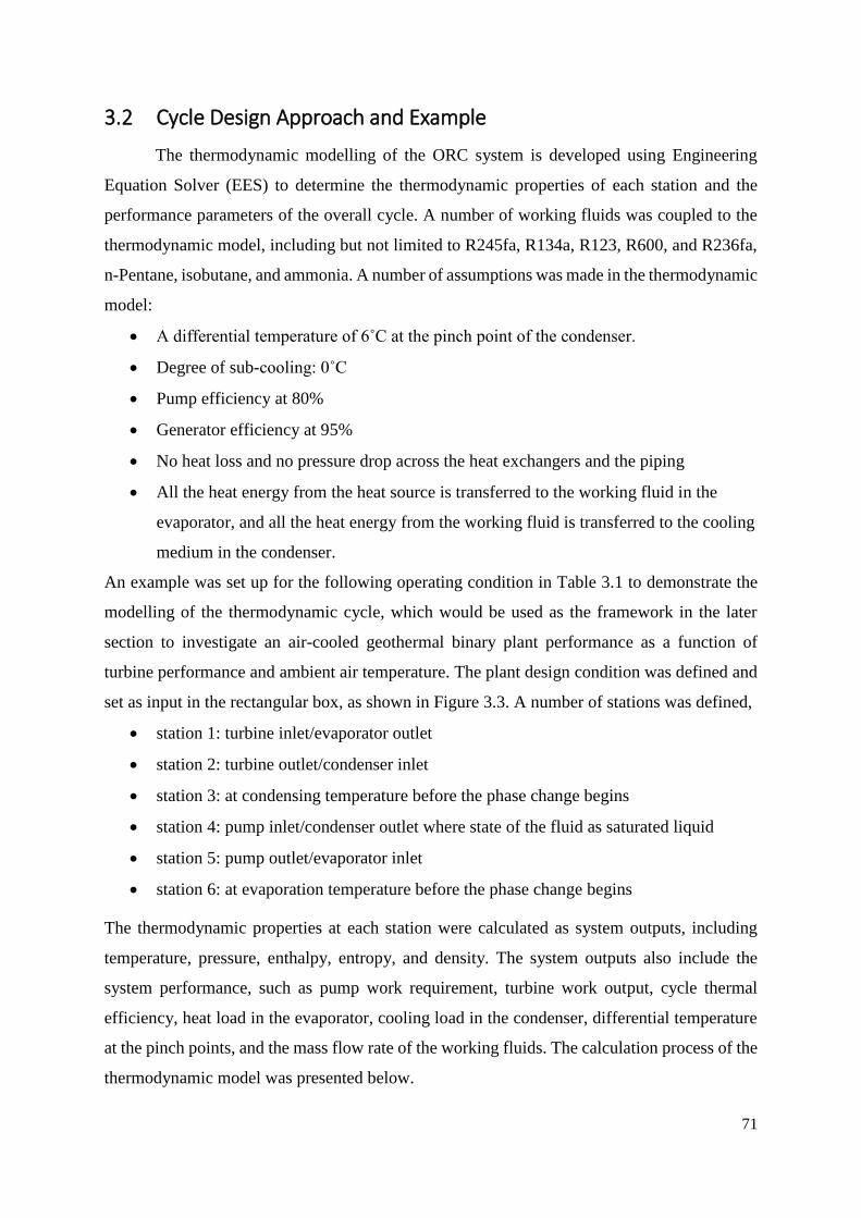
71
3.2 Cycle Design Approach and Example
The thermodynamic modelling of the ORC system is developed using Engineering
Equation Solver (EES) to determine the thermodynamic properties of each station and the
performance parameters of the overall cycle. A number of working fluids was coupled to the
thermodynamic model, including but not limited to R245fa, R134a, R123, R600, and R236fa,
n-Pentane, isobutane, and ammonia. A number of assumptions was made in the thermodynamic
model:
A differential temperature of 6˚C at the pinch point of the condenser.
Degree of sub-cooling: 0˚C
Pump efficiency at 80%
Generator efficiency at 95%
No heat loss and no pressure drop across the heat exchangers and the piping
All the heat energy from the heat source is transferred to the working fluid in the
evaporator, and all the heat energy from the working fluid is transferred to the cooling
medium in the condenser.
An example was set up for the following operating condition in Table 3.1 to demonstrate the
modelling of the thermodynamic cycle, which would be used as the framework in the later
section to investigate an air-cooled geothermal binary plant performance as a function of
turbine performance and ambient air temperature. The plant design condition was defined and
set as input in the rectangular box, as shown in Figure 3.3. A number of stations was defined,
station 1: turbine inlet/evaporator outlet
station 2: turbine outlet/condenser inlet
station 3: at condensing temperature before the phase change begins
station 4: pump inlet/condenser outlet where state of the fluid as saturated liquid
station 5: pump outlet/evaporator inlet
station 6: at evaporation temperature before the phase change begins
The thermodynamic properties at each station were calculated as system outputs, including
temperature, pressure, enthalpy, entropy, and density. The system outputs also include the
system performance, such as pump work requirement, turbine work output, cycle thermal
efficiency, heat load in the evaporator, cooling load in the condenser, differential temperature
at the pinch points, and the mass flow rate of the working fluids. The calculation process of the
thermodynamic model was presented below.

72
Table 3.1: Design condition of a geothermal binary plant (similar to the design condition of Rotokawa steam field
in New Zealand [7])
Heat source condition
Working medium - Geothermal brine (modelled as water/steam)
Mass flow rate kg/s 84.17
Inlet pressure kPa 2400
Inlet temperature °C 217.5
Injection well temperature °C 150
Binary cycle
Working medium - n-Pentane
Degree of superheat (turbine inlet) °C 3
Turbine inlet temperature °C 120
Heat sink condition
Cooling mechanism - mechanical draft using air-cooled condenser
Cooling medium - air
Ambient temperature °C 17
Figure 3.3: Graphical user interface of an ORC model developed by the author

73
Heat source:
The enthalpy of the heat source at the inlet and the outlet of the evaporator was determined by
calling the in-built functions based on the given temperature and pressure. The geothermal
brine was modelled as water/steam in this study. The heat rate absorbed by the working fluid
from the geothermal brine was determined using equation (3.11).
,1 ,2H gb gb gbQ m h h (14.11)
Where ṁgb is the mass flow rate of brine, HQ is the total heat rate transferred from the
geothermal brine into the binary loop, and hgb,1 and hgb,2 are the enthalpy of brine at the
evaporator inlet and outlet, respectively. All the heat energy was assumed to be transferred to
the working fluid within the evaporator without losses into atmosphere or conduction losses
into the piping. The mass flow rate of the working fluid in the binary loop (or the ORC system)
was determined using equation (3.12).
1 5/ ( )wf Hm Q h h (14.12)
Where ṁwf is the mass flow rate of the working fluid, and h1 and h5 are the enthalpy of the
working fluid at the evaporator inlet and the outlet, respectively.
Pinch point at the evaporator:
The pinch point in the evaporator was determined at station 6 (refer to Figure 3.4). The energy
balance between the geothermal brine and the working fluid at the pinch point allows the
calculation of the pinch point of the geothermal brine. The enthalpy at the pinch point of the
geothermal brine was determined using equation (3.13).
1 6
, ,1
wf
gb pinch gb
gb
m h hh h
m
(14.13)
The temperature at the pinch point of the brine, Tgb,pinch was determined using the in-built
property function as a function of enthalpy and pressure. The pinch point temperature
difference is set at 5˚C to ensure a feasible heat exchange within the evaporator.
,evap evap gb pinchT T T (14.14)

74
Where ΔTevap is the pinch point temperature difference of the evaporator.
Heat sink:
The required heat to be rejected into the atmosphere was calculated using equation (3.6). The
cooling load is equivalent to the required to be rejected into the atmosphere, assuming no loss
of heat into the atmosphere and no heat gain by the piping. The required mass flow of the
cooling air was determined using equation (3.15).
, ,
condair
p air air outlet ambient
Qm
C T T
(14.15)
Where ṁair is the mass flow of the cooling air, Cp,air is the isobaric specific heat of air, and
Tair,outlet is the outlet temperature of the cooling air, which was set at 35˚C in this example.
Pinch point at the condenser:
Pinch point at the condenser was determined at station 3 (refer to Figure 3.4). The energy
balance equation was applied within the condenser, and the temperature of the cooling medium
at the pinch point was determined using equation (3.16).
3 4
,pinch
,
( )wf
cond ambient
air p air
m h hT T
m c
(14.16)
Where Tcond,pinch is the temperature of the cooling medium at the pinch point. The pinch point
temperature difference of the condenser was set at 6˚C to allow feasible heat transfer between
the cooling medium and the working fluid of the ORC system.
,cond cond cond pinchT T T (14.17)
Where Tcond is the condensation temperature of the working fluid within the binary loop (or the
ORC system), and ΔTcond is the pinch point temperature difference of the condenser.

75
Binary cycle (or Organic Rankine Cycle):
Station 1: The thermodynamic properties at the turbine inlet were determined by using the in-
built property functions.
Station 2: The pressure ratio across the turbine was set up as the ratio of the evaporation
pressure (station 6) and condensation pressure (station 3). The turbine isentropic efficiency was
assumed 85%, and the enthalpy at the turbine outlet was determined using equation (3.4). The
other properties of interest (density, entropy, etc.) were then determined using the in-built
functions.
Station 3: The condensation temperature was determined using the aforementioned pinch point
analysis, and the condensation pressure was determined as the saturation pressure of the
working fluid at the condensation temperature. The enthalpy and the entropy were determined
using the in-built functions at the saturated vapour state (where the quality is one).
Station 4: The condenser outlet was determined at the saturated liquid state where the quality
of the working fluid is zero.
Station 5: The pump efficiency was assumed 80%, and equation (3.7) was used to determine
the pump outlet condition given that the pump outlet pressure is the same as the evaporation
pressure, assuming no pressure drop across the piping.
Station 6: The evaporation temperature was determined given the turbine inlet temperature and
the degree of superheat. The other thermodynamic properties were then determined by calling
the appropriate look-up functions, as discussed previously.

76
System performance:
The auxiliary power requirement includes the fan power in the air-cooled condenser. The fan
motor power requirement was determined using equation (3.18).
air airfan
fan motor
V pW
(14.18)
Where airV volumetric flow rate of air, Δpair is pressure drop of cooling air across the fan, ηfan is
fan efficiency and ηmotor is motor efficiency. The pressure drop of the air across the fan was
assumed 170 Pa [8], the fan efficiency and the motor efficiency were assumed 80% and 95%,
respectively.
The work output of the turbine was determined using equation (3.5), and the work requirement
of the pump was calculated using equation (3.5). The thermal efficiency and exergy efficiency
were calculated using equations (3.9) and (3.10). The system output was presented in Figure
3.3 and the temperature-entropy diagram was illustrated in Figure 3.4.
Figure 3.4: Temperature-entropy diagram of the binary plant model using n-Pentane
0.0 0.3 0.5 0.8 1.0 1.3 1.5 1.8
50
100
150
200
s [kJ/kg-K]
T [
°C]
1
2
34 5
6 7
1
2
1
2
brinebrine
working fluid (n-Pentane)working fluid (n-Pentane)
cooling medium (air)cooling medium (air)

77
3.3 References
This section provides the fundamental thermodynamic modelling of the ORC system.
This component is crucial in the SMC-DTR approach as this component is coupled to the SMC
adaptive strategy to perform iterative calculations in order to determine the optimal
configuration of the available turbines and the working fluid for optimal cycle performance.
3.4 References
1. DiPippo, R., Geothermal power plants: principles, applications, case studies and
environmental impact. 2012: Butterworth-Heinemann.
2. Lazzaretto, A. and G. Manente, A New Criterion to Optimize ORC Design Performance
using Efficiency Correlations for Axial and Radial Turbines. International Journal of
Thermodynamics, 2014. 17(3).
3. Ghasemi, H., et al., Modeling and optimization of a binary geothermal power plant.
Energy, 2013. 50(0): p. 412-428.
4. Span, R., Multiparameter equations of state: an accurate source of thermodynamic
property data. 2000: Springer.
5. Tarjan, R., Depth-first search and linear graph algorithms. SIAM journal on
computing, 1972. 1(2): p. 146-160.
6. Klein, S.A. and G. Nellis, Mastering EES. 2013: F-Chart Software.
7. Legmann, H. and P. Sullivan. The 30 MW Rotokawa I geothermal project five years of
operation. in International Geothermal Conference. 2003.
8. Lukawski, M., Design and optimization of standardized organic Rankine cycle power
plant for European conditions. 2010.

78
4.0 Define Turbine
Specification

79
The aim of this thesis is to present the SMC-DTR approach for low temperature
resources, and the main contribution of this thesis is to develop the key component, SMC
adaptive strategy. This chapter presents the approach to define the specification for radial
inflow turbine: calculating the shaft speed, turbine wheel diameter, and number of stages using
a standard turbine specific speed-specific diameter performance chart. Three screening criteria,
namely tip speed, shaft speed, and relative Mach number at the turbine outlet were defined to
calculate the number of stages. Four different case studies were presented and the specification
of the radial inflow turbine was determined for the case studies. The case studies include a 1
kW ORC-B pilot plant installed in University of Canterbury, a planned bottoming cycle in
Refining NZ, an ORMAT binary plant in Rotokawa geothermal field, and two installed
commercial ORC units (known as PureCycle) in Chena hot spring.

80
4.1 Introduction
Once the thermodynamic cycle has been established, the type of turbine and expander
has to be selected before the turbine specification is defined. The type of turbine and expander
can be specified using the specific speed-specific diameter by Balje, as shown in Figure 4.1
[1]. This method is commonly used to select a suitable type of gas turbine, steam turbine and
hydraulic turbine [2, 3]. Another turbine selection chart has been developed by Quoilin [4] to
select the working fluid and the type of turbine for LT-ORC. The performance map is
applicable for three different turbines: screw expander, scroll expander, and radial inflow
turbines. However, the selection of the turbine type would not be presented in this thesis as the
method does not form part of the SMC-DTR approach. The SMC-DTR approach in this thesis
utilizes radial inflow turbine, and the reasons were presented in Chapter 1.
Figure 4.1: Turbine performance chart by Balje as a function of specific speed and specific diameter [1]
This chapter aims to present the approach to define the specification of radial inflow
turbine for LT-ORC application by considering shaft speed, turbine tip speed, and relative
Mach number at the turbine outlet. A relative Mach number less than one is recommended to

81
ensure a subsonic expansion across the turbine, as a supersonic flow would impose an
additional shock loss during the expansion process [5], further reducing the isentropic
efficiency of the turbine. A high shaft speed would impose high friction loss at the bearing and
the coupling. A high shaft speed (equivalent to a high tip speed) also gives rise to a high
centrifugal stress on the turbine rotor and shaft, increasing the fatigue stress and the failure
probability. The specification of the radial inflow turbine was defined for four different case
studies: a 1 kW ORC-B pilot plant installed in University of Canterbury, a planned bottoming
cycle in Refining NZ, an ORMAT binary plant in Rotokawa geothermal field, and two installed
commercial ORC units (known as PureCycle) in Chena hot spring.

82
4.2 Calculation of Shaft Speed and Turbine Diameter
The turbine shaft speed and the turbine diameter can be calculated using the specific
speed-specific diameter turbine performance chart. The concept of specific speed has been
introduced first in year 1903 [6] as an important parameter for turbine blade design. The
concept was applied by Balje to correlate the turbine performance data as a function of specific
speed and specific diameter, as illustrated in Figure 4.1. The concept of specific speed was then
applied by Wood (reported in the work by Dixon [7]), Whitfield [8] and Baines [3] to correlate
the efficiency of axial turbines and radial inflow turbines to specific speed. The specific speed
is a non-dimensional parameter which is proportional to shaft speed and independent of turbine
geometry, as shown in equation (4.1).
0.75
exit
s
isen
m
Nh
(15.1)
Where Ns is the specific speed, ω is turbine shaft speed in rad/s, ṁ is mass flow across the
turbine stage, ρexit is fluid density evaluated at the turbine outlet, and Δhisen is the isentropic
enthalpy drop.
The specific diameter is another non-dimensional parameter which is dependent on the turbine
geometry and independent of the shaft speed.
0.25
isen
s
exit
D hD
m
(15.2)
Where Ds is the specific diameter, and d is the turbine rotor diameter. The feasible operating
range of specific speed and the corresponding specific diameter of radial inflow turbine is
shown in Table 4.1. The turbine shaft speed and the rotor diameter can be determined using
equations (4.1) and (4.2) once the specific speed and the specific diameter have been selected
from Table 4.1.
Table 4.1: Optimal specific speed and the corresponding specific diameter for radial inflow turbine
Specific speed, Ns Specific diameter, Ds Potential maximum efficiency Note
0.2 8 0.8 Feasible
0.5 4 0.9 Optimal
0.8 3 0.8 Feasible

83
4.3 Calculation of Number of Stages
The required pressure ratio determines the number of stages of turbine. A high pressure
ratio across a turbine is favorable to generate a high amount of work output. However, if the
pressure ratio is too high for the individual turbine stage, a supersonic expansion would occur
within the turbine. The shock wave is formed and the isentropic efficiency of the turbine is
compromised. If the design pressure ratio for the individual turbine stage is too low, the
required number of stages would increase, and the system cost would escalate to an
unacceptable value. A balance has to be achieved to obtain a high pressure ratio across each
turbine stage and a minimal number of turbine stages with an acceptable range of isentropic
efficiency.
The number of stages can be determined using the flow chart illustrated in Figure 4.3.
A suitable value of pressure ratio (usually less than 5.0) is guessed. The specific speed and
specific diameter are selected from Figure 4.1 or from Table 4.1. The turbine shaft speed, the
turbine diameter and the tip speed are calculated. Tip speed is one of the important factors to
determine the centrifugal loading on the turbine wheel. The centrifugal stress can be
approximated using equation (4.3).
2
material inK U (15.3)
Where σ is centrifugal stress on the turbine rotor, K is the geometrical factor, ρmaterial is the
density of the material of the turbine rotor, and Uin is rotor inlet tip speed. If the centrifugal
stress is more than the yield strength of the selected material, the turbine blade would suffer
structural failure and fatigue issue. A limiting turbine tip speed of 400 m/s is used in the
calculation process.
The relative Mach number at the turbine outlet is then calculated. If the relative Mach
number is over 1, a supersonic expansion would occur within the rotor blade passage, inducing
the shock loss and reducing the isentropic efficiency of the turbine stage. The relative Mach
number can be calculated using equation (4.4).
,
exitrel exit
critical
WMa
C
(15.4)
Where Marel,exit is the relative Mach number at the turbine outlet, Wexit is the relative flow
velocity at the turbine outlet, and Ccritical is the local speed of sound at the turbine outlet. The
relative flow velocity, Wexit is determined from a velocity triangle (shown in Figure 4.2), which

84
is commonly used in turbomachinery application to determine the vector of the bulk flow at
the inlet and the outlet of the fluid machines. The following assumption are made to facilitate
the calculation procedure:
Zero swirl at the turbine outlet, where Cθ is 0 [7]
Flow coefficient, ϕ is 0.2 based on the flow coefficient-loading coefficient chart
compiled by Baines [9]
Inlet to outlet radius ratio, rr is chosen as 1.8 (usually in the range of 1.6 and 18) [7]
Figure 4.2: Velocity diagram at the rotor inlet and outlet
The relative flow velocity, Wexit is the simplified from the unknown variables of the velocity
vectors, into the known variables, including the flow coefficient, and radius ratio, as stated in
equation (4.5).
2 2 2
, ,
2 2 2 2
( )
(1/ ) 0.35
exit m exit exit exit
in r in
W C C U
U r U
(15.5)
Where Cm is absolute flow velocity in meridional plane across the turbine, Cθ is absolute
tangential flow velocity, and the subscript exit is the turbine outlet. More information of the
velocity triangle can be referred to a number of relevant texts [3, 7, 10]. The limiting value of
relative Mach number is set at 0.95 to avoid the supersonic expansion within the blade passage.
If the relative Mach number is over 0.95, the pressure ratio of the current stage is re-selected.
The calculation is iterated until the total pressure ratio is equivalent to the required total
pressure ratio of the system. The process flow of the calculation is illustrated in Figure 4.3.
α2 β2
U2
W2
C2 C
m2
Cθ2
Wθ2
β3
α3
U3
W3
C3
Cθ3
Cm3

85
Figure 4.3: Flow chart calculating the number of stages for radial inflow turbine
Given fluid and turbine
operating condition
Select specific speed and
specific diameter from Figure
4.1
Calculate shaft speed, turbine
diameter, and tip speed
Tip speed
< 400m/s
Relative Mach
number<0.95
Pr = Prn x Prn-1 x …. x Pr1, where
Pr is pressure ratio
YES
NO
YES
NO
Select the pressure ratio for
current stage (nth stage)
Calculate relative Mach number at
turbine outlet
Pr < required total
pressure ratio
Determine the total
number of stages
YES
NO

86
4.4 Case Studies for Turbine/Expander Selection
The calculation process (Figure 4.3) was applied in four different case studies: 1 kW
ORC-B pilot plant in University of Canterbury, a planned bottoming cycle in a refinery plant,
a proposed binary plant for a high temperature steam field, and a binary plant for a low
temperature geothermal hot spring. The heat source condition, cooling medium, and the
operating condition of the corresponding ORC system were tabulated in Table 4.2. The 1 kW
ORC-B pilot plant in University of Canterbury is a bottoming cycle of a 30 kW Capstone gas
turbine, built by ORC research team between year 2013 and 2014 in University of Canterbury
using a commercially available scroll expander from Air Squared supplier. The plant utilizes a
non-conventional working fluid, a mixture of R365mfc and R245fa, to match the thermal curve
of the exhaust gas from the gas turbine. The waste heat recovery system using the kerosene
flow in Refinery plant in New Zealand is a conceptual study by ORC research team from
University of Canterbury. The conceptual study aims to evaluate the feasibility of an ORC
plant as a bottoming cycle in an existing chemical process plant. The Rotokawa steam field in
New Zealand utilizes a hybrid plant configuration, with a combination of steam plants and
binary plants as the bottoming cycles. The Chena hot spring in Alaska, United States utilizes a
commercially available ORC unit, known as PureCycle from Pratt and Whitney (at the time of
writing) to extract the low temperature heat energy.
The methodology, as outlined in Figure 4.3, was applied for different cases to determine
the shaft speed, turbine diameter, turbine tip speed, and number of stages for different
applications, and the result was tabulated in Table 4.3. The numerical model was applied in
Microsoft Excel and the mathematical equations were solved. The calculated shaft speed of the
turbine was compared to the actual rotational speed of the radial inflow turbine in Chena hot
spring to validate the outlined method. The actual shaft speed of the radial inflow turbine in
Chena hot spring is 13,500 rev/min whereas the optimal value based on the proposed method
is 13,123 rev/min. Radial inflow turbine are not currently installed in the 1 kW ORC-B pilot
plant due to the excessive shaft speed to achieve an acceptable turbine efficiency in a feasible
range of specific speed.

87
Table 4.2: Resource characteristics and operating parameters for the ORC system
Application Waste heat recovery Waste heat
recovery [11]
High temperature
geothermal [12]
Low temperature
geothermal [13]
Site
University
Canterbury 1 kW
ORC-B Pilot Plant,
New Zealand
Refining NZ,
New Zealand
Rotokawa
Geothermal Field,
New Zealand
Chena Hot spring,
Alaska, US
Heat Source
Heat source
medium Exhaust gas Kerosene flow Geothermal brine Hot spring water
Heat source inlet
temperature (ᵒC) 300.0 115.0 217.5 73.3
Heat source outlet
temperature (ᵒC) 230.0 70.0 150.0 54.4
Mass flow (kg/s) 0.11 40.3 84.17 33.39
Heat sink
Cooling medium Water Water Air Water/Air
Cooling medium
temperature (ᵒC) 15.50 24.00 12.00 4.44
ORC system
Working medium
M1 (mixture of
R365mfc and
R245fa)
R245fa n-Pentane R134a
Mass flow (kg/s) 0.07 17.8 46.122 12.17
Density at turbine
outlet (kg/m3) 6.15 13.17 2.622 20.84
Pressure ratio 11.0 3.0 17.622 3.6
Enthalpy drop
(kJ/kg) 34.30 17.13 112.252 22.15
Turbine
efficiency 0.851 0.851 0.97 0.8
Nominal Power
(kW) 2.0 259.2 5,021.7 215.7
1The turbine efficiency was estimated at 85% for the subsequent analysis. 2The operating condition was estimated based on the given heat source condition and nominal power output of
the turbo-generator unit, by using the energy balance formulae as described by DiPippo [14].

88
Table 4.3: Turbine specifications for the case studies
Site University Canterbury 1
kW ORC-B Pilot Plant Refining NZ
Rotokawa Geothermal
Field
Chena Hot
spring
Candidate 1
Machine type Radial inflow turbine
N (rev/min) 145,791 6,902 5,736 13,123
Actual N (rev/min) NIL NIL NIL 13,500*
D (m) 0.029 0.39 0.68/0.98 0.24
U (m/s) 218.1 141.5 204/294 164.4
Ma_rel 0.8882 0.604 0.6/0.79 0.6515
Ns 0.5 0.5 0.35/0.65 0.5
Number of stages 1 1 2 1
*The calculated rotational speed from the aforementioned numerical model was compared to the actual rotational
speed of the steam/binary plant.
4.5 Conclusion
The proposed method is one of the critical steps in the SMC-DTR approach to define
the turbine specification. This method is validated and can be fed into the next component to
design the optimal geometry of the turbine, before a suitable turbine can be selected from a
pool of turbine options.

89
4.6 References
1. Balje, O.E., Turbomachines: A Guide to Design Selection and Theory. 1981: Wiley.
2. Kenneth, E. and P. Nichols, How to select turbomachinery for your application. Barber-
Nichols Inc, 2012: p. 5-6.
3. Japikse, D. and N.C. Baines, Introduction to turbomachinery. 1995: Concepts ETI.
4. Quoilin, S., S. Declaye, and V. Lemort, Expansion Machine and fluid selection for the
Organic Rankine Cycle. 2010.
5. Dahlquist, A.N., Investigation of Losses Prediction Methods in 1D for Axial Gas
Turbines, in Division of Thermal Power Engineering, Department of Energy Sciences.
2008, Lund University: Sweden.
6. Meher-Homji, C.B. ‘The Historical Evolution of Turbomachinery. in Proceedings of
the 29th Turbomachinery Symposium, Texas A&M University, Houston, TX. 2000.
7. Dixon, S.L. and C. Hall, Fluid Mechanics and Thermodynamics of Turbomachinery.
2010, Butterworth-Heinemann: Burlington.
8. Whitfield, A. and N.C. Baines, Design of radial turbomachines. 1990.
9. Chen, H. and N.C. Baines, The aerodynamic loading of radial and mixed-flow turbines.
International Journal of Mechanical Sciences, 1994. 36(1): p. 63-79.
10. Schobeiri, M., Turbomachinery flow physics and dynamic performance. 2005:
Springer.
11. Jung, H.C., S. Krumdieck, and T. Vranjes, Feasibility assessment of refinery waste
heat-to-power conversion using an organic Rankine cycle. Energy Conversion and
Management, 2014. 77(0): p. 396-407.
12. Legmann, H. and P. Sullivan. The 30 MW Rotokawa I geothermal project five years of
operation. in International Geothermal Conference. 2003.
13. Aneke, M., B. Agnew, and C. Underwood, Performance analysis of the Chena binary
geothermal power plant. Applied Thermal Engineering, 2011. 31(10): p. 1825-1832.
14. DiPippo, R., Geothermal power plants: principles, applications, case studies and
environmental impact. 2012: Butterworth-Heinemann.

90
Investigative Study
5.0 Preliminary Design of
Radial Inflow Turbine

91
The aim of this thesis is to present the SMC-DTR approach for low temperature
resources, and the main contribution of this thesis is to develop the key component, SMC
analysis approach. One of the critical steps in the SMC-DTR approach is to match existing
turbines to the cycle design with different working fluid. This step is accomplished by
performing a preliminary design of radial inflow turbine based on the selected working fluid
and the turbine specification from previous chapters. The preliminary design approach provides
the optimal geometry of the radial inflow turbine for a given resource condition. A suitable
turbine (similar to the optimal geometry) is then selected from a pool of off-the-shelf turbines,
such as gas turbines and automotive turbochargers. The standard preliminary design approach
assumes ideal gas behaviour and provides good design outcomes for gas turbines and
turbochargers when the working medium is air, but the method is proven not suitable for real
fluids [1]. For ORC working fluids, it is not known how the ideal gas assumption affects the
preliminary design outcome. The previous research shows that the deviation of thermodynamic
properties is up to 100% in terms of local speed of sound and Mach number for refrigerants
such as R245fa [2].
In this chapter the standard preliminary design approach was developed using ideal and
real gas behaviour and the results were compared and analysed. The turbine preliminary design
and analysis was performed using two different gas models, which are ideal gas equations, and
multi-parameters equations of states for real fluids. The ideal gas equations in this chapter
assumes constant values of isobaric specific heat and specific heat ratio for all temperature.
Three working fluids are selected, R134a, R245fa and n-Pentane as they are the common
refrigerants in low temperature ORC system and geothermal binary plant.
The results show that the deviation in change in enthalpy across the turbine stage using
ideal gas equations is significant up to 1,000% when the compressibility factor is further away
from one. The shape of the velocity diagram is dependent on the selection of turbine
performance parameters, such as flow coefficient and radius ratio, but the shape of the velocity
diagram is not affected by the choice of the gas models. The application of the ideal gas model
over-estimates the turbine rotational speed and flow velocity, and under-sizes the rotor wheel
diameter. The over-estimation in the turbine rotational speed using the ideal gas model
increases the enthalpy loss across the turbine significantly, to the extent that the loss is larger
than the isentropic enthalpy drop across the turbine. The turbine operates as a pump and
consumes power for operation instead of operating as a turbine. The study shows that the

92
turbine preliminary design using real gas model is a better option to design the radial inflow
turbine or to match the existing turbines to the cycle design.

93
5.1 Introduction
The turbine design conditions are usually specified by a steady state model of a
thermodynamic cycle for the chosen working fluid. Standard turbomachinery design methods
are typically used to calculate turbine geometry for this steady state “design point” [3-5]. The
ideal gas assumption is applied throughout the conventional 1-D turbine preliminary design
and analysis process to reduce the computational effort. However, the properties of refrigerants
and organic fluids deviate significantly from ideal gas behaviour. The ideal gas equations have
been shown to result in an extremely large deviation, in the range of 18% up to over 100% in
terms of Mach number, thermodynamic properties, fluid sound velocity and total pressure loss
across the turbine [23-25]. There are a number of methods to estimate the real fluid properties
in the numerical calculation process [25], which are
(a) interpolation and extrapolation of thermodynamic property data tables,
(b) application of simple polynomial functions to fit the data of the property data tables
from approach (a),
(c) analytical method to calculate the primitive quantities and a numerical scheme to
evaluate the derivatives of the primitive values, and
(d) analytical method to calculate both the primitive quantities and the derivative values
Method 4 has been shown to provide the highest accuracy results, followed by 3, 2 and 1 [25].
The first two methods result in lower accuracy attributed to errors in the data interpolation.
Two common equations of states (EoS) for real fluids are Redlich-Kwong-Soave (RKS)
equations and Peng Robinson (PR) equations. A study by Lujan showed that the RKS and PR
equations exhibit deviations of 8% and 6% respectively from the specific energy across the
range of interest for R245fa compared to the NIST fluid property database [23]. Harinck
studied the deviation of an improved version of the PR model by Stryjek and Vera, known as
PRSV cubic equation from a highly accurate multi-parameter equation of state (MPEoS) [25].
He considered three different fluids, which are steam, toluene and R245fa in his study. He
found that adopting the PRSV model for toluene and R245fa results in 2% deviations and 4%
deviations for steam in all the flow parameters. Lemmon and Roland have developed the
equations of states for a number of fluids, including non-polar fluids (carbon monoxide,
decane, neopentane, toluene, isopentane, isohexane, etc.) and polar fluids (R134a, R245fa,
R41, acetone, etc.) using Helmholtz energy equations with the experimental data [6, 7]. The

94
equation of states is known as multi-parameter equations of states with 12 coefficients to fit
the experimental data with the mathematical model.
The numerical calculation of the turbine preliminary design process and performance
estimation has been implemented in the commercially available thermodynamic software,
namely Engineering Equations Solver (EES), with in-built fluid properties database to model
the behaviour of the real fluids. Some research were previously performed to improve the
turbine preliminary design process by coupling the preliminary design with external fluid
database [8]. The turbine preliminary design process has been integrated into ORC system
design to optimize the overall cycle performance with a proper selection of turbine parameters
and turbine geometry [9]. A turbine designed using perfect gas equations and tested using real
fluids was shown by Kang [4]. A single stage radial turbine was designed using dry air as
working fluid with a pressure ratio of 3.6 with isentropic efficiency of 75%. The prototype of
the turbine was built and tested using R245fa for a pressure ratio between 2.5 and 2.8, with
tested isentropic efficiency between 60 and 80% [4].
This chapter aims to present the radial inflow turbine preliminary design method to
match the existing turbines to the cycle design. The conventional preliminary design method
using ideal gas model might not be suitable to provide an optimal turbine design outcome.
Therefore, this chapter compares the turbines designed using the ideal gas equations and multi-
parameter equations of states. The deviation in the performance parameters for turbines
designed using ideal gas equations and multi-parameter equations of states for real fluids is
then correlated to the compressibility factor at the turbine inlet condition.

95
5.2 Standard Preliminary Design Approach
This section presents the preliminary design of the radial inflow turbine using 1)
polytropic ideal gas equations, and 2) multi-parameter equations of states by integrating the
turbine preliminary program to a fluid database. The turbine performance analysis was
presented as enthalpy loss in terms of passage loss, incidence loss, exit kinetic energy loss, tip
clearance loss, and windage loss. The turbine loss model was validated against a gas turbine
using air and an ORC turbo-expander using R245fa at the operating condition close to the
design condition. The numerical model was developed using Engineering Equation Solver
(EES) as EES is able to solve non-linear mathematical equations using the in-built Newton’s
method algorithm, and the in-built fluid database can be integrated into the turbine design and
analysis program for better thermodynamics accuracy in the modelling process. 3 different
stations were defined: station 1, nozzle inlet; station 2, rotor inlet; station 3: rotor outlet. The
turbine design and analysis method was presented assuming the absence of diffuser
downstream of the rotor. The velocity diagram at the rotor inlet and outlet was illustrated in
Figure 5.1, which was applied in the preliminary design process to develop the velocity
diagram at different stations. C denotes absolute flow velocity, W relative flow velocity, U
turbine tip speed, α absolute flow angle (also known as swirl angle), β relative flow angle, Cm
absolute flow velocity projected onto meridional plane, and Cθ absolute flow velocity projected
onto tangential direction.
Figure 5.1: Velocity diagram at the rotor inlet and outlet
α2 β2
U2
W2
C2 C
m2
Cθ2
Wθ2
β3
α3
U3
W3
C3
Cθ3
Cm3

96
5.2.1 Preliminary Design
The preliminary design approach of radial inflow turbine is crucial in defining the
optimal geometry of the turbine. A suitable turbine can then be selected from a pool of off-the-
shelf turbines with the turbine geometry similar to the optimal geometry. The standard turbine
preliminary design process has been discussed, improved and presented by a number of
researchers [10-16] for the past few decades since the publication of the computational code of
turbine preliminary design program as part of the NASA gas turbine program by Glassman
[17].
The flow coefficient-stage loading coefficient correlation chart serves as a first step in
the turbine preliminary design approach. The correlation between the flow coefficient and stage
loading coefficient of radial section blades has been compiled by Baines using the actual test
data of the radial inflow turbines [18]. Flow coefficient determines the swallowing capacity of
the turbines whereas stage loading coefficient (sometimes known as work coefficient)
determines the non-dimensional work output of the turbines. Flow coefficient, ϕ is the ratio of
absolute flow velocity in the meridional plane, Cm3, to the rotor inlet tip speed, U2.
3
2
mC
U (16.1)
Stage loading coefficient, ψ is the ratio of total enthalpy drop across the turbine, Δh0 to the
squared to rotor inlet tip speed.
0 2 3
2
2 2
h C C
U U
(16.2)
Where Cθ2 is the flow velocity in the tangential direction at the rotor inlet, and Cθ3 is the flow
velocity in the tangential direction at the rotor outlet. This equation is simplified as a function
of the flow velocity and rotor radius ratio, ε=r3/r2. The radius ratio was reported to be in the
range of 0.4 to 0.75 for centrifugal compressors to achieve a high pressure ratio across the
turbine stage [19].The radius ratio is limited below 0.7 to avoid excessive curvature of the rotor
shroud [20].
The stage loading coefficient is selected between 0.9 and 1.0, and the flow coefficient
is selected in the range of 0.2 and 0.3 to achieve optimal turbine efficiency. The stage loading
coefficient-flow coefficient correlation chart is only valid for radial section blade with rotor
outlet blade angle, β3b at 0˚. If β3b is greater than zero, the optimal stage loading coefficient is

97
increased and the maximum turbine efficiency is achieved at lower velocity ratio. Velocity
ratio, υ is the ratio of rotor inlet tip speed to spouting velocity, Cs, which is defined as the flow
velocity if the flow is expanded in the same total-to-static pressure ratio as the turbine stage in
an ideal nozzle. The equation can be simplified to a function of rotor inlet tip speed and total-
to-static enthalpy drop in an isentropic expansion process, Δhts,is.
2 2
,2s ts is
U U
C h
(16.3)
If β3b is less than zero, the optimal stage loading coefficient is reduced and the maximum
turbine efficiency is achieved at higher velocity ratio [21]. The subsequent turbine preliminary
design process was presented assuming the radial section blades. The optimal velocity ratio is
around 0.7 for radial section blades [14].
The specific work output of a turbine is determined using Euler turbomachinery
equation.
0 2 2 3 3 2 2 2 2 3 3tan tanx m mW h U C U C U C U C (16.4)
WherexW is the specific work output. The specific work output would increase if the turbine
outlet swirl angle, α3 is negative. However, the negative swirl angle at the rotor outlet increases
the kinetic energy loss at the turbine outlet. The minimal kinetic energy loss at the rotor outlet
occurs at zero swirl angle, in which the absolute flow velocity at the rotor outlet is minimal.
The swirl angle, α3 is set as zero for this preliminary design approach.
The turbine wheel diameter and the rotational speed can be determined using the
specific speed-specific diameter performance chart in the previous chapter. The rotor inlet tip
is calculated using equation (5.5), in which d2 is the turbine wheel diameter, and N is the
rotational speed in rad/sec. The rotor outlet tip speed is calculated given the radius ratio (which
is set at 0.7).
22
60
d NU
(16.5)
3 2U U (16.6)
The isentropic total-to-static enthalpy change, Δhts,is can be deduced from the total-to-static
pressure ratio, prts specified as part of the requirement of turbine design condition.

98
1
, 01
11
kk
ts is p
ts
h C Tpr
(16.7)
Where Cp is the isobaric heat capacity, T01 is stagnation temperature at the turbine inlet, and k
is specific heat ratio.
The isentropic efficiency of the turbine stage is first guessed using the loading coefficient-flow
coefficient performance chart compiled by Baines [18]. The actual enthalpy drop is then
predicted using equation (5.8).
0 ,ts ts ish h (16.8)
Where Δh0 is the actual enthalpy drop across the turbine.
Rotor Exit:
The velocity diagram at the rotor exit is constructed. The absolute flow velocity in the
meridional plane is calculated using equation (5.1) and the tip speed is determined from
equation (5.6). The outlet swirl angle, α3 is set as zero. The velocity vector and the flow angle
in Figure 5.1 are calculated using equations (5.9) to (5.13).
3
3
3cos
mCC
(16.9)
3 3 3tanmC C (16.10)
3 3 3W C U (16.11)
2 2
3 3 3mW C W (16.12)
3
3
3
tanm
W
C
(16.13)
Rotor Inlet:
The velocity diagram at the rotor inlet is constructed. Cθ2 is calculated using the Euler
turbomachinery equation in equation (5.4). The meridional velocity at the rotor inlet, Cm2 is
assumed to be the same as the meridional velocity at the rotor outlet, Cm3. The other velocity
vectors and flow angle are calculated using equations (5.14) to (5.18).

99
2 2 2W C U (16.14)
2
2
2
tanm
W
C
(16.15)
2 2
2 2 2mC C C (16.16)
2
2
2
tanm
C
C
(16.17)
2 2
2 2 2mW C W (16.18)
5.2.2 Thermo-physical and Thermodynamic Properties
The calculation of the thermodynamic properties of the refrigerants is crucial in the
design process. Polytropic ideal gas equations are usually employed for the design of
conventional gas turbine and turbocharger as the polytropic ideal gas law can predict the
thermodynamic properties of air accurately. The ideal gas law assumes constant isobaric
specific heat and constant specific heat ratio for the range of temperature studied in this chapter.
The application of different working medium in ORC system, such as hydrocarbon and
hydrofluorocarbon, requires real gas model to predict the thermodynamic properties accurately.
The thermodynamic properties of the real gas can be determined from the original Redlich-
Kwong equation [22] or the modified version of Redlich-Kwong equation [11]. In this study,
the real gas fluid database from Engineering Equation Solver (EES) is integrated into the
turbine preliminary design code developed by the author. The real fluid model in this study is
based on the multi-parameter equation of states, which is described later.
5.2.3 Perfect Gas Model
The averaged specific heat ratio, k is determined given the turbine inlet and the
isentropic outlet operating condition. The isobaric heat capacity, Cp is assumed constant
throughout the expansion process and calculated using the equation below.
1
p specific
kC R
k
(16.19)
Where Rspecific is the specific gas constant for the working fluid.
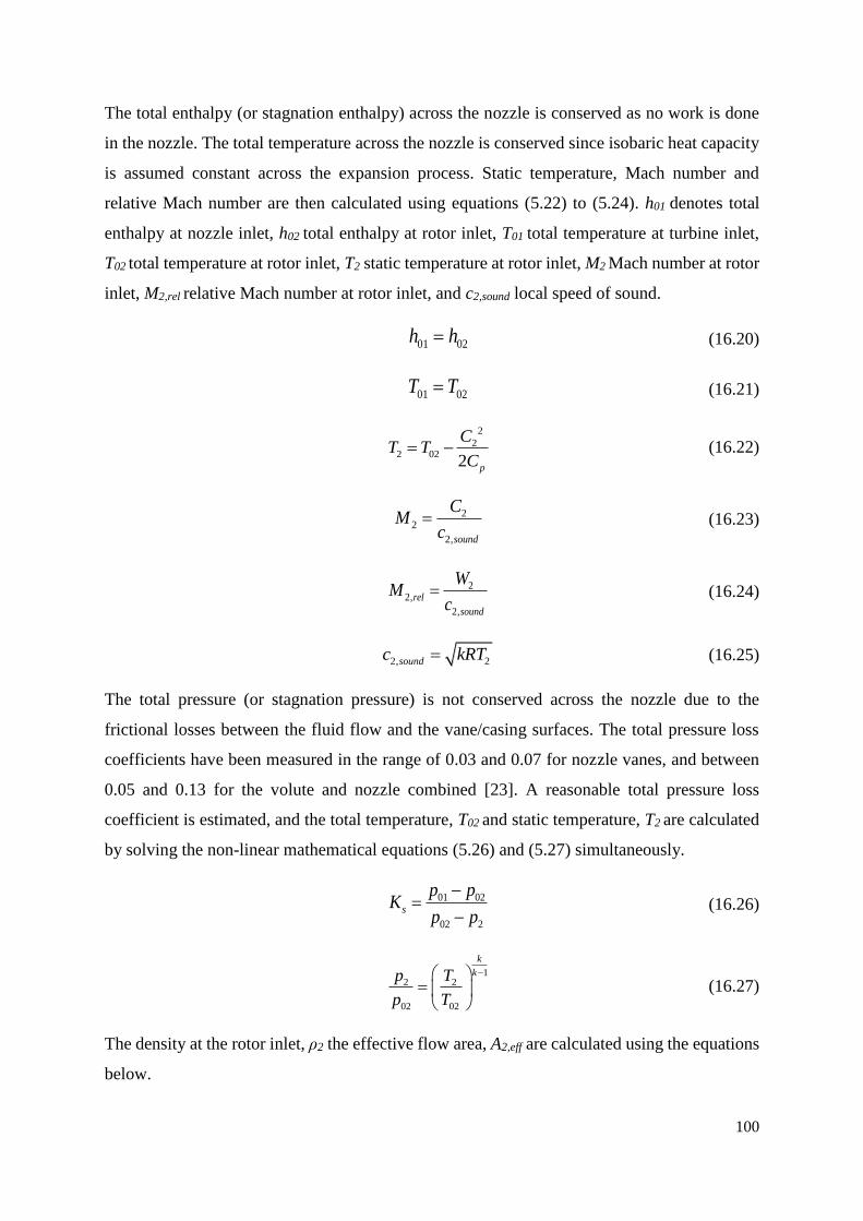
100
The total enthalpy (or stagnation enthalpy) across the nozzle is conserved as no work is done
in the nozzle. The total temperature across the nozzle is conserved since isobaric heat capacity
is assumed constant across the expansion process. Static temperature, Mach number and
relative Mach number are then calculated using equations (5.22) to (5.24). h01 denotes total
enthalpy at nozzle inlet, h02 total enthalpy at rotor inlet, T01 total temperature at turbine inlet,
T02 total temperature at rotor inlet, T2 static temperature at rotor inlet, M2 Mach number at rotor
inlet, M2,rel relative Mach number at rotor inlet, and c2,sound local speed of sound.
01 02h h (16.20)
01 02T T (16.21)
2
22 02
2 p
CT T
C (16.22)
2
2
2,sound
CM
c (16.23)
2
2,
2,
rel
sound
WM
c (16.24)
2, 2soundc kRT (16.25)
The total pressure (or stagnation pressure) is not conserved across the nozzle due to the
frictional losses between the fluid flow and the vane/casing surfaces. The total pressure loss
coefficients have been measured in the range of 0.03 and 0.07 for nozzle vanes, and between
0.05 and 0.13 for the volute and nozzle combined [23]. A reasonable total pressure loss
coefficient is estimated, and the total temperature, T02 and static temperature, T2 are calculated
by solving the non-linear mathematical equations (5.26) and (5.27) simultaneously.
01 02
02 2
s
p pK
p p
(16.26)
1
2 2
02 02
k
kp T
p T
(16.27)
The density at the rotor inlet, ρ2 the effective flow area, A2,eff are calculated using the equations
below.

101
2
2
2
P
RT (16.28)
2,
2 2
eff
m
mA
C (16.29)
The losses within the vaneless zone between the nozzle vanes and the rotor is ignored in this
study. The thermodynamic properties at the rotor outlet are calculated using equations (5.30)
to (5.34). Mass conservation equation is applied to estimate the effective flow area at the
turbine outlet, A3,eff.
0
03 01
p
hT T
C
(16.30)
2
33 03
2 p
CT T
C (16.31)
1
3 3
03 03
k
kp T
p T
(16.32)
3
3
3,sound
CM
c (16.33)
3
3,
3,
rel
sound
WM
c (16.34)
3,
3 3
eff
m
mA
C
(16.35)
5.2.4 Real Gas Model
The thermodynamic properties of the real gas are calculated using multi-parameter
equations of states in EES. The equation of state of real fluids are expressed in fundamental
form explicit in the Helmholtz energy as a function of density and temperature. The Helmholtz
energy is split into two terms, one to describe the behaviour of ideal gas at given density and
temperature, and one to consider the residual behaviour of the real fluid [7], as shown in
equation (5.36). The first term on the right hand side is the contribution from hypothetical ideal
gas model, in which the internal energy of molecules are attributed to the translational,

102
rotational, vibrational, and intramolecular motion. The second term accounts for all
intermolecular interactions. The residual Helmholtz energy is usually measured and
determined from the experimental data due to the lack of physics model that can be fitted into
the whole spectrum of real fluids.
0( , ) ( , ) ( , )ra T a T a T (16.36)
The functional form of Helmholtz energy is usually expressed in the dimensionless form, as a
function of dimensionless density and temperature, where δ=ρ/ρc and τ=Tc/T. α denotes
dimensionless Helmholtz energy, ρC critical density, and Tc critical temperature.
0( , )( , ) ( , ) ( , )ra T
RT
(16.37)
The functional form of the residual of Helmholtz energy term is expressed in two different
forms, one for polar fluids (R134a and R245fa), in equation (5.38), and one for non-polar fluids
(n-Pentane and hydrocarbon), in equation (5.39). They both are represented by twelve
coefficients, which have to be determined empirically. e is the exponential term, and the
coefficients (n1,n2,….,n12) for R134a, R245fa, and n-Pentane can be found by the works by
Roland [7] and Eric [6], respectively.
2 2 2 3
0.25 1.25 1.5 3 0.25 7 0.875 2.375 2 2.0
1 2 3 4 5 6 7
5 2.125 3.5 6.5 4 4.75 2 12.5
8 9 10 11 12
( , ) e e
e e e e e
r n n n n n n n
n n n n n
(16.38)
2 2 3 3
0.25 1.125 1.5 2 1.375 3 0.25 7 0.875 2 0.625
1 2 3 4 5 6 7
5 1.75 3.625 4 3.625 3 14.5 4 12.0
8 9 10 11 12
( , ) e
e e e e e
r n n n n n n n
n n n n n
(16.39)
The thermodynamic properties, such as compressibility factor, internal energy, enthalpy,
entropy, heat capacity, and speed of sound, can be determined as a function of the derivatives
of Helmholtz energy, in which the full mathematical models can be found from the works by
Span [7] and Eric [6].
The numerical model in the preliminary design phase is similar to the numerical model
shown using polytropic ideal gas law, but most of the thermodynamic properties are determined
as a function of enthalpy and entropy. The total enthalpy and entropy at the turbine inlet are
determined using the total temperature and total pressure at the turbine inlet. The isentropic
enthalpy at the turbine outlet, h3,is is determined as a function of total entropy at turbine inlet,

103
s01 and static pressure at the turbine outlet, p3. The isentropic total-to-static enthalpy drop, Δhts,is
is determined using equation (5.43).
01 01 01( , )h f T p (16.40)
01 01 01( , )s f T p (16.41)
3, 3 1( , )ish f p s (16.42)
, 01 3,ts is ish h h (16.43)
The total enthalpy across the nozzle is conserved, hence h02=h01, and the static enthalpy
at the nozzle outlet is determined from equation (5.44). The nozzle loss coefficient, ξs is
expressed in term of static enthalpy loss, as shown in equation (5.45). The nozzle enthalpy loss
coefficient has been found between 0.05 and 0.15 by Benson as a function of corrected mass
flow [24]. The overall stage performance, however, is insensitive to the nozzle loss coefficient
in this range [12]. The isentropic enthalpy at the nozzle outlet, h2,is is determined by selecting
an appropriate value of the nozzle loss coefficient. The pressure at the nozzle outlet, ps is
determined as a function of nozzle inlet entropy and nozzle outlet isentropic enthalpy. The
other thermodynamic properties (T2, ρ2, c2,sound) are then determined by calling the property
function in EES as a function of pressure, p2 and enthalpy, h2.
2
2 02 2
1
2h h C (16.44)
2 2, 2 2,
202 22
1
2
is is
s
h h h h
h hC
(16.45)
2 2, 2 1 01 2,( , )is isp p f s s s h (16.46)
The turbine loss in the vaneless zone between the nozzle and the rotor is neglected, and the
thermodynamic properties at the nozzle outlet are assumed the same as the thermodynamic
properties at the rotor inlet. The effective flow area at the nozzle outlet and the rotor inlet are
estimated using equation (5.29). The total enthalpy at the rotor outlet is determined using the
Euler turbomachinery equation. The rothalpy, I is total enthalpy (or stagnation enthalpy) in
rotating frame of reference. The rothalpy is constant along the streamlines of the flow path
within a radial turbine [10]. The conservation of rothalpy within the rotor allows the calculation

104
of static enthalpy at the turbine outlet, h2 once the velocity diagram at the turbine outlet is
constructed. The static pressure at the turbine outlet is defined by user. The thermodynamic
properties (T3, ρ3, s3, csound) are determined as a function of static pressure, p3 and static
enthalpy, h3. The total entropy and the static entropy at the turbine outlet is the same (s03=s3).
The total (or stagnation) condition at the turbine outlet are determined as a function of entropy,
s3 and total enthalpy, h03.
03 01 0h h h (16.47)
2 2 2 2
3 3 3 3 2 2 2 2
1 1 1 1
2 2 2 2I h W U I h W U (16.48)
5.2.5 Nozzle and Rotor Design
The rotor and nozzle geometry are set up based on the constructed velocity diagram
and the thermodynamic properties from the previous section. The effective flow area at the
rotor inlet and the outlet are calculated using equations (5.29) and (5.35). The aerodynamic
blockage fraction, B is assumed as 0.02 to take account into the thin boundary layer by the fluid
flow. The geometrical flow area, Aeff is then calculated using equation (5.49). The blade height
at the rotor inlet, b2, the rotor outlet tip diameter, r3,shroud and the hub diameter, r3,hub are
determined by using a value of radius ratio, ε in the range of 0.4 and 0.7, where ε=r3/r2.
1
eff
geo
AA
B
(16.49)
2, 2 22geoA r b (16.50)
2 2
3, 3, 3,geo shroud hubA r r (16.51)
The nozzle vane is designed and set up using the correlations presented by Glassman
[25] and Aungier [11]. The nozzle vane is uncambered and the vane height is constant across
the nozzle stage. The nozzle inlet-to-outlet ratio is recommended to be 1.25 [25]. Nozzle inlet
flow angle is usually assumed to be radially inward in the preliminary design stage [10] but
this is not the optimal case. Nozzle inlet flow angle, α1 is calculated using the correlation by
Glassman, shown in equation (52), where cs is the chord of nozzle vane, and r3 is the mean
radius at the rotor outlet. The chord of the nozzle vane is calculated using equation (5.53),
which is derived mathematically from the work by Glassman [17]. The equation is only valid

105
if the vane surface length is equivalent to the chord length, which is applicable for uncambered
vanes.
2
1
2
2
sintan
cossc
r
(16.52)
2
2 2 2
12 22 cos 0s sc r c r r (16.53)
The correlation between minimum number of nozzle vane for zero diffusion loss, nozzle exit
angle, nozzle inlet angle, and radius ratio was plotted by Northern Research and Engineering
Corporation and reported by Baines [12]. The number of nozzle vane can be predicted using
the aforementioned correlation chart. The pitch (or vane spacing) at the nozzle outlet is
estimated given the nozzle vane number, Zs.
2
2
2
s
rs
Z
(16.54)
The width of nozzle throat, os is then estimated using cosine rule [11].
2
2
cos so
s (16.55)
The clearance gap between the nozzle outlet and the rotor inlet correlates to the turbine
efficiency. The optimal clearance gap was proposed by proposed by Watanabe as a function of
nozzle blade height, b2 and outlet flow angle, α2 [26].
2 22 cos r b (16.56)
One of the challenges in turbine design is the estimation of number of blades. If the number of
blade is excessive, the blade surface area is high and the frictional loss is high [15]. A minimum
number of blade is necessary to avoid flow reversal [27]. There are different equations to
calculate the minimum number of rotor blades developed by Jamieson [27], Glassman [16]
and Whitfield [15]. Glassman suggested that Jamieson’s equation provides an excessive
number of rotor blades especially at high stator exit flow angles [28]. Whitfield’s equation for
number of blades is developed for minimum rotor inlet Mach number [15], as shown in
equation (57). The empirical correlation between number of rotor blades and the nozzle outlet
angle, derived by Glassman [25] in equation (5.58) is employed. The number of blades can

106
also be deduced using the empirical correlation by Rohlik [29] as a function of absolute flow
angle in equation (5.59), as presented by Aungier [11].
2
2
0.63
2cosrZ
(16.57)
2 2110 tan
30rZ
(16.58)
2
212 0.03(33 )rZ (16.59)
The mean blade pitch at the rotor outlet, s3 and the width of throat, or can be estimated using
the following equations [11]. If the relative Mach number at the rotor outlet, M3,rel is less than
one (implying a subsonic expansion process), the throat width can be deduced using equation
(5.61).
3
3
2
r
rs
Z
(16.60)
3 3
3r
ms Co
W (16.61)
5.2.6 Turbine Loss Model
The performance losses of radial turbine were categorized into stator loss, rotor loss,
clearance loss, windage loss, and exit kinetic energy loss by Rohlik [29].Different breakdown
of loss models were proposed and developed over the years for radial turbine, such as stator
loss, incidence loss, and viscous loss within rotor by Glassman [25], profile loss, incidence
loss, clearance loss, blade loading effect, hub-to-shroud loading effect, and moisture loss by
Aungier [11], incidence loss, passage loss, clearance loss, trailing edge loss, and windage loss
by Baines [12]. The subsequent turbine loss model was mainly adapted from the turbine loss
model suggested by Baines but the passage loss model presented by Venture was applied [3].
Passage loss is defined as total loss within the blade passage, including secondary flow
loss, mixing flow loss, blockage loss, and kinetic energy loss due to the growth of boundary
layer along the blade surface [12]. Baines reported that the initial passage loss model by NASA
cannot accurately predict the passage loss for all types of radial turbines under different
operating conditions. An improved version of passage loss formula is presented in his work

107
based on the geometry at the throat of the impeller. However, the evaluation of the fluid flow
velocity at the throat is difficult as the blade profile is usually not finalized in the preliminary
design stage. The passage loss model in this study is evaluated as the average value of
Musgrave loss model and Rodgers loss model [3], which considers the rotor inherent curvature
and frictional effects.
2
22 21
22
hpassage t
h c r
L r Ch f W
D r Z
(16.62)
The passage loss coefficient is expressed in term of enthalpy loss, where ft is skin friction factor
modified by Musgrave for curved flow inside the rotor, Lh is the hydraulic length, Dh is the
hydraulic diameter, Ŵ is the averaged value of the relative fluid flow velocity evaluated at rotor
inlet and outlet, rc is the mean curvature radius and Zr is the blade number of the impeller. The
parameters in equation (5.62) are found by solving the equations (5.63) to (5.66), where f is
Fanning friction factor and Re is Reynolds number. The mean curvature radius, rc is assumed
as the mean radius of the flow passage, and calculated using equation (5.67).
2 2
3, 3,2 2
2 2 3, 3, 3, 3,
41
2 2
shroud hub
h
r shroud hub r shroud hub
r rr bD
r Z b r r Z r r
(16.63)
22
3, 3,22 3,
1
2 2 2 2
shroud hub
h shroud
r rbL r r
(16.64)
0.251 0.075Re
2
hc
c
Df f
r
(16.65)
0.052
Re int c
c
rf f
r
(16.66)
2 3cr r r (16.67)
Incidence loss occurs when the fluid approaches the rotor at an angle differs from the
optimal flow angle. The optimal relative flow angle, β2,opt is determined by the empirical
correlation by Whitfield in equation (5.68) [15]. The incidence loss coefficient is calculated as
the change in relative flow velocity in tangential direction [30], as expressed in equation (5.69),
where n is 3 at positive incidence and 2 at negative incidence angle based on the experimental
result by Glassman [17] (as reported by Baines in [12]).

108
2
2
,
1.98tan
1.981
opt
r
r
tan
ZZ
(16.68)
2 2,2
1sin
2incidence o t
n
ph W
(16.69)
A common loss of energy in turbomachinery is the kinetic energy of the fluid flow at
the rotor outlet. If the swirl angle is large at the turbine outlet, the internal energy of the fluid
is converted into the kinetic energy where the magnitude of the energy is proportional to the
square of the absolute flow velocity at the turbine outlet. A diffuser is commonly employed to
recover the kinetic energy into the static pressure rise of the fluid at the stage outlet given that
the installation space is not a design constraint. The enthalpy loss of the flow at the rotor outlet
is expressed as below.
2
3
1
2exith C (16.70)
A clearance gap exists between the rotor and the casing/housing, which is categorized
as axial clearance and radial clearance. The axial clearance is the gap between the rotor and the
housing at the rotor inlet whereas the radial clearance is the gap between the rotor and the
housing at the outlet. The tip clearance is modelled as an orifice with shear flow inside the
passage [30]. The clearance loss is expressed in term of enthalpy loss in equation (5.71). and
the mathematical derivation of the equation can be found from the work by Baines [12].
2,
3
(8
rtip a a a r r r a r a r a r
U Zh K C K C K C C
(16.71)
Where Ka is the discharge coefficient of the axial component, Kr is the discharge coefficient of
the radial component, Ka,r is the cross coupling coefficient of the axial and radial components,
εa is the axial clearance gap, and εr is the radial clearance gap. The values of Ka, Kr, and Ka,r
are found as 0.4, 0.75, and -0.3, respectively, with good agreement with experimental data [12].
Ca and Cr are axial and radial coefficients for tip clearance model with the following equations.
3,
2
m2 2
1
b
shr
a
oudr
r
CC
(16.72)

109
3, 2
2 m3 3 3r b
shroud totalr
r b b
r CC
(16.73)
Windage loss is frictional loss between the back face of the rotor and the fluid flow
leaked into the gap between the back face of the rotor and housing/generator. The leakage flow
acts as a counter-rotating flow and generates a frictional torque on the back face of the rotor.
The fluid flow behaviour in the region was investigated by Daily and Nece [31] by considering
a rotating disc in an enclosed casing. The empirical equations were modified to consider the
frictional torque on the rotor, and expressed in enthalpy loss, as shown in equation (5.74).
3 2
2 2
2windage f
U rh k
m
(16.74)
kf denotes the empirical correlation for frictional torque by Daily and Nece [31], and ρ is the
mean fluid density evaluated by rotor inlet and outlet static condition. The correlation is
dependent on Reynolds number and the value is calculated for two different flow regimes,
laminar flow (Re<105) using equation (5.75), and turbulent flow (Re>105) using equation
(5.76). ε denotes the clearance gap between the back face of the rotor wheel and the housing.
0.1
2
0.5
3.7
Ref
rk
(16.75)
0.1
2
0.2
0.102
Ref
rk
(16.76)
The turbine total-to-static efficiency, ηts and total-to-total efficiency, ηtt are then determined
as below.
0
0
ts
passage incidence tip windage
h
h h h h h
(16.77)
0
0
tt
passage incidence tip windage exit
h
h h h h h h
(16.78)

110
5.2.7 Validation of Turbine Empirical Loss Model
The turbine loss model was developed based on a number of existing correlations for
air from different authors. The passage loss model was validated by Emilie [3] and compared
against the improved passage loss model by Baines [12]. However, the lack of published data
with detailed measurement of properties of interest inside the blade passage makes the
validation of the individual loss models difficult. Also, the other loss models (incidence loss,
windage loss and tip clearance loss) are validated against the data from the radial turbines with
low pressure ratio gas turbine and turbocharger [12]. At the time of writing, there were no
published loss models specifically developed for refrigerants. Thus, the loss models for air
were used for the performance analysis for refrigerants and validated by comparison to
published turbine performance data for air [32] and R245fa [4].
The design parameters from a commercial gas turbine unit and an academic research
turbo-expander unit are presented in Table 5.1 for the validation purpose. The numerical model
in this study does not take into account of the losses across the nozzle. Whitfield [15] reported
that the overall turbine performance is very insensitive to the nozzle loss coefficients based on
the potential range of nozzle loss coefficients calculated by Benson [24] and Johnston [33].
The simulated turbine total-to-static efficiency from the turbine empirical loss model and the
turbine efficiency at the design point are shown in Table 5.1. The turbine empirical loss model
over-estimates the turbine performance in the range of 2 to 4%. The discrepancy is attributed
to the lack of loss coefficients of the nozzle and the vaneless space between rotor and nozzle.
However, the turbine model is sufficient to provide an estimation of the potentially highest
turbine efficiency in this study assuming that the nozzle is designed properly with minimal
losses.
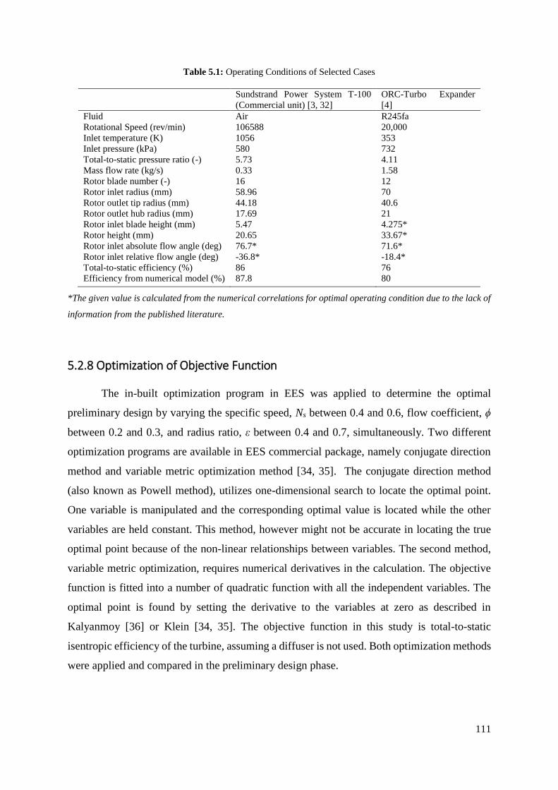
111
Table 5.1: Operating Conditions of Selected Cases
Sundstrand Power System T-100
(Commercial unit) [3, 32]
ORC-Turbo Expander
[4]
Fluid Air R245fa
Rotational Speed (rev/min) 106588 20,000
Inlet temperature (K) 1056 353
Inlet pressure (kPa) 580 732
Total-to-static pressure ratio (-) 5.73 4.11
Mass flow rate (kg/s) 0.33 1.58
Rotor blade number (-) 16 12
Rotor inlet radius (mm) 58.96 70
Rotor outlet tip radius (mm) 44.18 40.6
Rotor outlet hub radius (mm) 17.69 21
Rotor inlet blade height (mm) 5.47 4.275*
Rotor height (mm) 20.65 33.67*
Rotor inlet absolute flow angle (deg) 76.7* 71.6*
Rotor inlet relative flow angle (deg) -36.8* -18.4*
Total-to-static efficiency (%) 86 76 Efficiency from numerical model (%) 87.8 80
*The given value is calculated from the numerical correlations for optimal operating condition due to the lack of
information from the published literature.
5.2.8 Optimization of Objective Function
The in-built optimization program in EES was applied to determine the optimal
preliminary design by varying the specific speed, Ns between 0.4 and 0.6, flow coefficient, ϕ
between 0.2 and 0.3, and radius ratio, ε between 0.4 and 0.7, simultaneously. Two different
optimization programs are available in EES commercial package, namely conjugate direction
method and variable metric optimization method [34, 35]. The conjugate direction method
(also known as Powell method), utilizes one-dimensional search to locate the optimal point.
One variable is manipulated and the corresponding optimal value is located while the other
variables are held constant. This method, however might not be accurate in locating the true
optimal point because of the non-linear relationships between variables. The second method,
variable metric optimization, requires numerical derivatives in the calculation. The objective
function is fitted into a number of quadratic function with all the independent variables. The
optimal point is found by setting the derivative to the variables at zero as described in
Kalyanmoy [36] or Klein [34, 35]. The objective function in this study is total-to-static
isentropic efficiency of the turbine, assuming a diffuser is not used. Both optimization methods
were applied and compared in the preliminary design phase.

112
5.2.9 Numerical Mathematical Model
The mathematical model of the preliminary design phase was defined and solved using
Engineering Equation Solver (EES), and the numerical model is shown in Figure 5.2. The
operating condition across the turbine is defined using the thermodynamic model in previous
chapter, and the shaft speed and the rotor diameter are calculated using the specific speed-
specific diameter chart. The design parameters (ϕ, ε) are selected using experience. An initial
guess for turbine efficiency is made and iterated to a final solution. The velocity diagram is set
up at the rotor inlet and rotor outlet, and the thermodynamic properties at each station are
calculated. The principal turbine geometry is then determined before the performance
evaluation. Two different optimization methods are then conducted by varying the specific
speed, Ns, flow coefficient ϕ, and radius ratio, ε. Turbine total-to-static efficiency is defined as
the objective function in the optimization program to select the best configuration of Ns, ϕ, ε
for further development.
Figure 5.2: Calculation flow for turbine preliminary design process
Select design parameters
(ϕ, ε)
Guess-estimate turbine
efficiency, η
Construct velocity diagram
assuming α3 is zero
Determine thermodynamic
properties at each station
Determine principal
geometry (r2, r3, α1, b2, b3,
Zs, Zr, os, or)
Performance evaluation
using empirical loss model
and calculate turbine
efficiency
Optimization by varying Ns,
ϕ, ε
Select a turbine geometry
η
converges?
No Yes
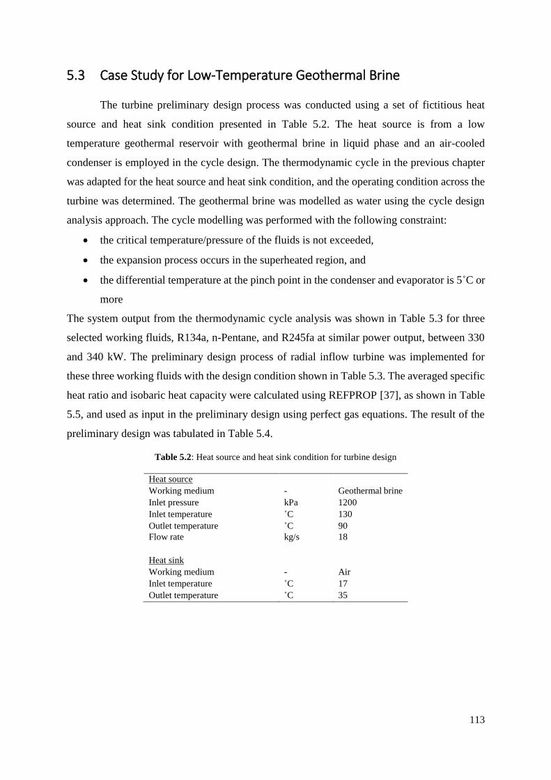
113
5.3 Case Study for Low-Temperature Geothermal Brine
The turbine preliminary design process was conducted using a set of fictitious heat
source and heat sink condition presented in Table 5.2. The heat source is from a low
temperature geothermal reservoir with geothermal brine in liquid phase and an air-cooled
condenser is employed in the cycle design. The thermodynamic cycle in the previous chapter
was adapted for the heat source and heat sink condition, and the operating condition across the
turbine was determined. The geothermal brine was modelled as water using the cycle design
analysis approach. The cycle modelling was performed with the following constraint:
the critical temperature/pressure of the fluids is not exceeded,
the expansion process occurs in the superheated region, and
the differential temperature at the pinch point in the condenser and evaporator is 5˚C or
more
The system output from the thermodynamic cycle analysis was shown in Table 5.3 for three
selected working fluids, R134a, n-Pentane, and R245fa at similar power output, between 330
and 340 kW. The preliminary design process of radial inflow turbine was implemented for
these three working fluids with the design condition shown in Table 5.3. The averaged specific
heat ratio and isobaric heat capacity were calculated using REFPROP [37], as shown in Table
5.5, and used as input in the preliminary design using perfect gas equations. The result of the
preliminary design was tabulated in Table 5.4.
Table 5.2: Heat source and heat sink condition for turbine design
Heat source
Working medium - Geothermal brine
Inlet pressure kPa 1200
Inlet temperature ˚C 130
Outlet temperature ˚C 90
Flow rate kg/s 18
Heat sink
Working medium - Air
Inlet temperature ˚C 17
Outlet temperature ˚C 35

114
Table 5.3: Turbine operating condition using different working fluids
Parameters Unit Case 1 Case 2 Case 3
Working fluid - R134a R245fa n-Pentane
Turbine inlet temperature ˚C 105.0 100 98
Turbine inlet pressure kPa 3,667 1,266 563
Degree of superheat ˚C 9 0 0
Mass flow rate kg/s 16.3 13.7 6.8
Turbine outlet temperature ˚C 43.8 54.0 62.1
Turbine outlet pressure kPa 1,003 238 109
Pressure ratio - 3.7 5.3 5.2
Turbine work output kW 330 340 333
Cycle efficiency % 8.4 9.8 9.8

115
Table 5.4: Design output from the preliminary design program for three different working fluids using perfect
gas equations and real gas equations
R134a R245fa n-Pentane
Ideal Real Ideal Real Ideal Real
Δhts,is kJ/kg 281 25 159 31 105 61
N rev/min 104,122 16,026 36,862 10,596 18,066 12,137
d m 0.093 0.186 0.189 0.312 0.337 0.385
Velocity diagram
α1 degree 51 51 51 51 51 51
α2 degree 77 77 77 77 77 77
α3 degree 0 0 0 0 0 0
β2 degree -29 -28 -28 -28 -30 -30
β3 degree -63 -63 -63 -63 -63 -63
U2 m/s 509 156 365 173 319 245
U3 m/s 204 62 146 69 127 98
C2 m/s 463 143 335 158 289 222
C3 m/s 102 31 73 35 64 49
W2 m/s 117 35 82 39 74 56
W3 m/s 228 70 163 78 127 109
Thermodynamic Conditions
T02 K 378 375 373 371 371 370
T2 K 317 345 330 349 351 353
p02 kPa 3,546 3,440 1,217 1,173 538 525
p2 kPa 2,340 1,995 726 591 289 271
M2 - 2.2 1.1 2.0 1.2 1.4 1.1
T03 K 247 317 281 327 327 335
T3 K 244 316 279 326 326 334
p03 kPa 1,032 1,027 245 246 113 113
p3 kPa 1,003 1,003 238 238 109 109
ρ3 kg/m3 50 48 14 13 3 3
M3,rel - 1.2 0.5 1.1 0.6 0.7 0.6
Principal Geometry
r1 m 0.058 0.116 0.118 0.195 0.211 0.241
r2 m 0.047 0.093 0.095 0.156 0.168 0.193
r3 m 0.019 0.037 0.038 0.062 0.067 0.077
r3,shroud m 0.032 0.062 0.067 0.103 0.112 0.127
r3,hub m 0.005 0.013 0.009 0.022 0.023 0.027
b2 mm 6 9 9 13 14 16
btotal mm 20 41 37 66 71 82
Zs - 20 20 20 20 20 20
Zr - 15 15 15 15 15 15
ss mm 15 29 30 49 53 60
sr mm 8 16 16 26 28 32
os mm 3 6 7 11 12 13
or mm 3 7 7 12 13 14
Turbine Performance
ΣΔhloss kJ/kg 49.0 3.1 38.5 3.5 11.3 6.5
ηts - 0.82 0.87 0.76 0.88 0.89 0.89
ψ - 0.9 0.9 0.9 0.9 0.9 0.9
Optimal configuration
ϕ - 0.2 0.2 0.2 0.2 0.2 0.2
ε - 0.4 0.4 0.4 0.4 0.4 0.4
Ns 0.48 0.49 0.46 0.49 0.49 0.50

116
Table 5.5: Averaged specific heat ratio and isobaric heat capacity of the selected fluids with the corresponding
operating range
Unit R134a R245fa n-Pentane
k - 1.74 1.10 1.32
cp kJ/kg.K 1.75 2.02 1.29
The turbine rotational speed and rotor wheel size were determined by first defining the
optimal specific speed and specific diameter from the specific speed-specific diameter
performance chart. The isentropic enthalpy drop across the turbine was over-estimated at 72%
(n-Pentane), 413% (R245fa), and 1,000% (R134a) using ideal gas equations. The rotor
diameter was over-estimated at 12.5% (n-Pentane), 39% (R245fa), and 50% (R134a), and the
shaft speed was over-predicted at 50% (n-Pentane), 250% (R245fa), and 550% (R134a). The
velocity diagrams at the rotor inlet and rotor outlet are similar for all the working fluids despite
the operating condition. The magnitude of the velocity was over-estimated when ideal gas
equations are applied attributed to the over-estimated turbine rotational speed and tip speed.
The high turbine tip speed and flow velocity give rise to the high values of Mach number at the
nozzle outlet, M2 and the relative Mach number at the rotor outlet, M3,rel. The principal
geometry of the turbine (r, b, s, and o) using ideal gas equations was under-estimated up to
50%. The turbine loss model was applied to estimate the losses for each design, and the turbines
designed using ideal gas equations were found to have a very high enthalpy loss, at 100% (n-
Pentane), 1,000% (R245fa) and 1,400% (R134a) higher than the turbines designed using real
gas equations. The estimated turbine isentropic efficiency using the ideal gas equations is not
accurate attributed to the large error in the isentropic enthalpy drop across the turbine. The
performance parameters of the turbine designed using ideal gas equations were re-evaluated by
re-calculating the isentropic enthalpy drop using equations (5.40) to (5.43), the specific speed,
the loading coefficient using equation (5.2), the velocity ratio using equation (5.3), the static
enthalpy at the rotor outlet using equation (5.48), the density at the rotor outlet, the mass flow
rate at the rotor outlet, ṁoutlet using equation (5.35), and the turbine isentropic efficiency using
equation (5.77), and tabulated in Table 5.6. The actual specific speed for the turbines designed
using ideal gas equations deviates significantly from the optimal specific speed (which is in the
range of 0.4 and 0.6 for radial inflow turbines). The performance of radial turbine is sensitive
to the choice of specific speed. Hence, the turbines designed using ideal gas equations for
R134a show the highest turbine loss, followed by R245fa, and n-Pentane. The deviation of
enthalpy change for R134a using ideal gas equations is the largest. Hence, the stage loading

117
coefficient, the specific speed, and the velocity ratio, which are functions of enthalpy change,
are deviated significantly from the optimal values. The predicted mass flow rate at the turbine
outlet is 410.7 kg/s, which is deviated significantly from the design specification at 16.3 kg/s
for R134a. The isentropic efficiency for the turbines designed using ideal gas equations for
R134a and R245fa were not available since the enthalpy loss is much higher than the isentropic
enthalpy drop. This indicates that the turbines operate as pumps and work input is required to
achieve the specified rotational speed.
Table 5.6: Performance parameters for turbines designed using perfect gas equations
Unit R134a R245fa n-Pentane
Ns - 3.2 1.7 0.7
Ψ - 0.08 0.18 0.53
ν - 2.27 1.47 0.91
ṁoutlet kg/s 410.7 23.8 7.4
ηts (%) - - - 83
The thermodynamic properties, enthalpy, h, and isobaric heat capacity, cp are
independent of pressure using perfect gas equations whereas the enthalpy and the isobaric heat
capacity are dependent on temperature and pressure in real fluids. Comparison was made
between the distribution of enthalpy as a function of temperature and pressure in Figure 5.3.
The temperature-pressure-enthalpy diagram was generated using REFPROP [37] with the
multi-parameter equations of states, whereas the temperature-enthalpy diagram in Figure 5.3(b)
was generated using equation (5.79). The enthalpy of the real fluids in the superheated region
is between 460 and 490 kJ/kg using real gas equations, but the enthalpy of the perfect gas is
between 650 and 750 kJ/kg. The change in enthalpy across the same temperature ratio is 30
kJ/kg for real gas and 100 kJ/kg for perfect gas. The large error in estimating the change in
enthalpy was carried forward during the preliminary design phase, with a poor choice of turbine
option as the design outcome.
ph C T (16.79)
The estimation of isobaric heat capacity and change in enthalpy for real fluids can be performed
using the following equations [38]. Cv,ideal denotes ideal isochoric heat capacity, and V specific
volume.

118
2
, 2
V
p v ideal
p
p TC C T dV TpT
V
(16.80)
p
ph C T T p V
T
(16.81)
In an ideal gas condition, the integral and the derivatives are simplified using equations (5.82)
to (5.84), and the interaction between molecules are neglected.
2
20
Vp
dVT
(16.82)
p R
T V
(16.83)
2
p RT
V V
(16.84)
The deviation of cp using ideal gas equations and some real gas equations was investigated and
presented in the study by Lujan [38].
(a) (b)
Figure 5.3: Temperature-enthalpy diagram for R245fa using multi-parameters equations of states (a) and ideal
gas equations (b)
100
90
80
70
60 200 1,000 400 600 800
490 kJ/kg 480 kJ/kg
470 kJ/kg
460 kJ/kg
Tem
per
atu
re (
˚C)
Pressure (kPa)
Sub-cooled
Super-heated region
Saturated line
50 60 70 80 90 100650
670
690
710
730
750
Temperature (C)
Enth
alp
y (
kJ/k
g)

119
Large deviation was found in turbine parameters, such as specific speed, loading
coefficient, velocity ratio, from the optimal values for the turbine designed using ideal gas
equations. The largest deviation was found for R134a, followed by R245fa and n-Pentane. The
largest deviation was found to occur when the compressibility factor is further away from one.
The compressibility factor was shown in Table 5.7. The preliminary design using ideal gas
equations yields large error when the compressibility factor is low. Compressibility factor is
the ratio of actual volume of a gas to the ideal volume of the gas. When the compressibility
factor is low, the deviation in estimating the thermodynamic properties (including enthalpy,
isobaric heat capacity, and etc.) is large.
Table 5.7: Molecular weight and compressibility factor of the selected working fluids
Fluid Compressibility factor at inlet
n-Pentane 0.85
R134a 0.56
R245fa 0.75
The result shows that the turbine preliminary design using perfect gas equations is valid if the
compressibility factor is close to one, as shown by n-Pentane with compressibility factor of
0.85. If the compressibility factor is further away from one, the high deviation in
thermodynamic properties would be carried forward in the preliminary design process with a
poor design choice.

120
5.4 Conclusion
This chapter presents the preliminary design process of radial inflow turbines using
ideal gas equations and real gas equations by coupling the turbine preliminary design program
to the in-built fluid database in EES. Multi-variable optimization was performed during the
preliminary design phase to determine the best turbine geometry by varying the selected turbine
parameters, such as specific speed, flow coefficient, and radius ratio. The turbine preliminary
design program was utilized to design turbines for a geothermal binary plant using three
different working fluids, namely n-Pentane, R245fa and R134a. The results show that the rotor
diameter is under-estimated and the shaft speed is over-estimated for the turbines designed
using ideal gas equations. The large deviation is attributed to the error in estimating the
thermodynamic properties using ideal gas equations, and the deviation is larger at lower
compressibility factor. The optimal flow angle and relative flow angle are independent on the
type of gas model as they are function of turbine parameters, such as the user-defined flow
coefficient and specific speed. The turbine preliminary design process using perfect gas
equations is valid only if the compressibility factor is close to one. If the compressibility factor
is deviated from one, the preliminary design using real gas equations is required to avoid the
poor turbine design options. Since the turbine operating condition is usually away from one,
the turbine preliminary design using real gas model is a better option to match the existing
turbines to the cycle design.

121
5.5 References
1. Harinck, J., Super-and Transcritical Fluid Expansions, in Mechanical, Maritime and
Materials Engineering. 2010, Delft University of Technology.
2. Harinck, J., et al., Influence of thermodynamic models in two-dimensional flow
simulations of turboexpanders. Journal of turbomachinery, 2010. 132(1): p. 011001.
3. Ventura, C., et al., Preliminary Design and Performance Estimation of Radial Inflow
Turbines: An Automated Approach. Journal of Fluids Engineering-Transactions of the
Asme, 2012. 134(3).
4. Kang, S.H., Design and experimental study of ORC (organic Rankine cycle) and radial
turbine using R245fa working fluid. Energy, 2012. 41(1): p. 514-524.
5. Sauret, E. and A.S. Rowlands, Candidate radial-inflow turbines and high-density
working fluids for geothermal power systems. Energy, 2011. 36(7): p. 4460-4467.
6. Lemmon, E.W. and R. Span, Short fundamental equations of state for 20 industrial
fluids. Journal of Chemical & Engineering Data, 2006. 51(3): p. 785-850.
7. Span, R., Multiparameter equations of state: an accurate source of thermodynamic
property data. 2000: Springer.
8. Fiaschi, D., G. Manfrida, and F. Maraschiello, Thermo-fluid dynamics preliminary
design of turbo-expanders for ORC cycles. Applied Energy, 2012. 97: p. 601-608.
9. Pan, L. and H. Wang, Improved analysis of Organic Rankine Cycle based on radial
flow turbine. Applied Thermal Engineering, 2013. 61(2): p. 606-615.
10. Dixon, S.L. and C. Hall, Fluid Mechanics and Thermodynamics of Turbomachinery.
2010, Butterworth-Heinemann: Burlington.
11. Aungier, R.H., Turbine aerodynamics: axial-flow and radial-inflow turbine design and
analysis. 2006: ASME Press.
12. Moustapha, H., et al., Axial and Radial Turbines. 2003: Concepts Eti.
13. Khan, R.S.R.G.a.A.A., Axial Flow and Radial Flow Gas Turbines, in Turbomachinery:
Design and Theory. 2003, CRC Press.
14. Japikse, D. and N.C. Baines, Introduction to turbomachinery. 1995: Concepts ETI.
15. Whitfield, A. and N.C. Baines, Design of radial turbomachines. 1990.
16. Glassman, A.J., Turbine Design and Application. NASA SP-290. NASA Special
Publication, 1972. 290.
17. Wasserbauer, C.A. and A.J. Glassman, FORTRAN program for predicting off-design
performance of radial-inflow turbines. NASA Technical Paper, 1975(TN D-8063).
18. Chen, H. and N.C. Baines, The aerodynamic loading of radial and mixed-flow turbines.
International Journal of Mechanical Sciences, 1994. 36(1): p. 63-79.
19. Schobeiri, M., Turbomachinery flow physics and dynamic performance. 2005:
Springer.
20. Rohlik, H.E., Analytical determination of radial inflow turbine design geometry for
maximum efficiency. 1968.

122
21. Baines, N. ENGR408-ENME 627-S1 Special Topic in Engineering: Turbomachinery.
2014.
22. Redlich, O. and J. Kwong, On the Thermodynamics of Solutions. V. An Equation of
State. Fugacities of Gaseous Solutions. Chemical Reviews, 1949. 44(1): p. 233-244.
23. Hiett, G. and I. Johnston. Paper 7: Experiments Concerning the Aerodynamic
Performance of Inward Flow Radial Turbines. in Proceedings of the Institution of
Mechanical Engineers, Conference Proceedings. 1963. SAGE Publications.
24. Benson, R.S., A review of methods for assessing loss coefficients in radial gas turbines.
International Journal of Mechanical Sciences, 1970. 12(10): p. 905-932.
25. Glassman, A.J., Computer program for design analysis of radial-inflow turbines. 1976.
26. Watanabe, I., I. Ariga, and T. Mashimo, Effect of dimensional parameters of impellers
on performance characteristics of a radial-inflow turbine. Journal of Engineering for
Power, 1971. 93: p. 81.
27. Jamieson, A., The radial turbine. Gas turbine principles and practice, 1955.
28. Whitfield, A., The preliminary design of radial inflow turbines. J. Turbomach, 1990.
112: p. 50-57.
29. Rohlik, H.E., Analytical determination of radial inflow turbine design geometry for
maximum efficiency. 1968: National Aeronautics and Space Administration.
30. Ghosh, S.K., R. Sahoo, and S.K. Sarangi, Mathematical Analysis for Off-Design
Performance of Cryogenic Turboexpander. Journal of fluids engineering, 2011. 133(3).
31. Daily, J. and R. Nece, Chamber dimension effects on induced flow and frictional
resistance of enclosed rotating disks. Journal of Basic Engineering, 1960. 82: p. 217.
32. Jones, A.C., Design and Test of a Small, High Pressure Ratio Radial Turbine. Journal
of Turbomachinery, 1996. 118(2): p. 362-370.
33. Benson, R., Paper 16: An Analysis of the Losses in a Radial Gas Turbine. Proceedings
of the Institution of Mechanical Engineers, Conference Proceedings, 1965. 180(10): p.
41-53.
34. Klein, S.A. and G. Nellis, Mastering EES. 2013: F-Chart Software.
35. Klein, S. and F. Alvarado, EES manual. Middleton, Wisconsin, USA, 1999.
36. Kalyanmoy, D., Optimization for engineering design: Algorithms and examples. 2004:
PHI Learning Pvt. Ltd.
37. Lemmon, E.W., Huber, M.L., McLinden, M.O, NIST Standard Reference Database 23:
Reference Fluid Thermodynamic and Transport Properties-REFPROP, Version 9.1, in
National Institute of Standards and Technology. 2013, Standard Reference Data
Program: Gaithersburg.
38. Luján, J.M., et al., Model of the expansion process for R245fa in an Organic Rankine
Cycle (ORC). Applied Thermal Engineering, 2012. 40(0): p. 248-257.

123
Components of the SMC
Adaptive Strategy
6.0 Meanline Analysis of
Radial Inflow Turbine
124
The aim of this thesis is to present the SMC-DTR approach for low temperature
resources, and the main contribution of this thesis is to develop the key component, SMC
analysis approach. The critical components of the SMC-DTR approach is the SMC adaptive
strategy. One of the analysis techniques of the SMC adaptive strategy is the meanline analysis.
This chapter aims to present the turbine performance analysis using the meanline analysis. The
meanline analysis refers to the performance analysis along the mid-line (also known as mean-
line or centre-line) of the fluid along the flow passage. The thermodynamic properties are
determined along the meanline of the fluid flow at different locations, such as the turbine inlet
and the turbine outlet. The meanline analysis model consists of the empirical loss models which
have been developed by the turbine manufacturers and the researchers. The meanline analysis
model in this study is made up from the loss models developed by Baines and by Sauret. The
model is validated against two different turbines: an industrial gas turbine and an academic-
based ORC turbine using R245fa as working fluid. The meanline analysis model in this chapter
is the same as the turbine performance analysis model presented in the previous chapter. This
model is integrated into the preliminary design of radial inflow turbine and the SMC adaptive
strategy attributed to the accuracy and the simplicity of the analysis model with minimal
computational effort.

125
6.1 Introduction
Numerical modelling of turbine performance can be classified into meanline analysis,
two-dimensional fluid flow study, three-dimensional inviscid fluid flow analysis, and three-
dimensional viscous flow study. The meanline analysis has been commonly used to model the
turbine performance in turbine preliminary design process, performance evaluation process in
the preliminary stage and turbine retrofit process. This analysis model is commonly applied in
turbomachines, such as axial flow turbines, axial flow compressors, radial flow turbines, and
centrifugal compressors. The analysis model involves a number of different loss models,
involving the passage loss, incidence loss, clearance loss, moisture loss, shear loss, frictional
loss, and etc. Most of the individual loss models have been developed empirically with some
empirical coefficients, and validated against the experimental data. The development of the
loss models requires the experiences of the engineers and researchers, referred to the field as
knowledge-based engineering. Not all the loss models are required to model the turbomachines.
For example, moisture loss model is applied specifically for steam turbines if the quality of the
fluid is less than one during the expansion process. The moisture loss model is not required in
an ORC expansion if the expansion of the fluid occurs in the superheated region. Most of the
turbine loss models have been developed for axial flow turbomachines in the military
application during the Second World War. Some of the loss models have then been adapted
and validated for radial flow machines, such as incidence loss model. The passage loss model
of axial flow machine cannot be adapted for radial flow machines due to the difference of the
flow patterns for these two turbomachines.
Meanline analysis refers to the performance analysis along the centre-line of the flow
passage. The end-wall effect and near the end-wall effect are usually not considered in the
meanline analysis. This analysis provides the representative values for the thermodynamic
properties at the critical stations in a turbine stage, including nozzle inlet, interface between
nozzle and rotor, and rotor outlet. Sometimes, a volute and a diffuser analysis would be
included in the meanline analysis. The meanline analysis technique in this chapter is the same
as the turbine performance analysis technique presented in the previous chapter as part of the
preliminary design method of radial inflow turbine. The meanline analysis approach is
integrated into the preliminary design (in the previous chapter) and the SMC adaptive strategy
as this analysis model can estimates the overall turbine efficiency with close agreement to the
experimental data with minimal computational effort.

126
The objective of this chapter is to present the meanline analysis model used in the SMC
adaptive strategy, and validate the model against two different turbines: one industrial radial
gas turbine and an ORC radial turbine using R245fa as working fluid. This meanline analysis
model in the SMC strategy is implemented only if the performance data of the selected turbines
is not available.

127
6.2 Turbine Loss Model
The performance losses of radial turbine can be categorized into stator loss, rotor loss,
clearance loss, windage loss, and exit kinetic energy loss by Rohlik [1].Different breakdown
of loss models have been proposed and developed over the years for radial turbine, such as
stator loss, incidence loss, and viscous loss within rotor by Glassman [2], profile loss, incidence
loss, clearance loss, blade loading effect, hub-to-shroud loading effect, and moisture loss by
Aungier [3], incidence loss, passage loss, clearance loss, trailing edge loss, and windage loss
by Baines [4]. The subsequent turbine loss model was adapted from different turbine loss
model, including the incidence loss, passage loss, clearance loss, trailing edge loss, and
windage loss by Baines [4], and the passage loss model by Venture [5].
Passage loss is defined as total loss within the blade passage, including secondary flow
loss, mixing flow loss, blockage loss, and kinetic energy loss due to the growth of boundary
layer along the blade surface [4]. The initial passage loss model by NASA cannot accurately
predict the passage loss for all types of radial turbines under different operating conditions [4].
An improved version of passage loss formula has been presented [4] based on the geometry at
the throat of the rotor. However, the evaluation of the fluid flow velocity at the throat is difficult
as the blade profile is usually not finalized in the preliminary design stage. The passage loss
model in this study is evaluated as the average value of Musgrave loss model and Rodgers loss
model [5], which considers the rotor inherent curvature and frictional effects.
2
22 21
22
hpassage t
h c r
L r Ch f W
D r Z
(17.1)
The passage loss coefficient is expressed in term of enthalpy loss, where ft is skin friction factor
modified by Musgrave for curved flow inside the rotor, Lh is the hydraulic length, Dh is the
hydraulic diameter, Ŵ is the averaged value of the relative fluid flow velocity evaluated at rotor
inlet and outlet, rc is the mean curvature radius and Zr is the blade number of the impeller.
The parameters in equation (6.1) are found by solving the equations (6.2) to (6.6), where f is
Fanning friction factor and Re is Reynolds number. The mean curvature radius, rc is assumed
as the mean radius of the flow passage, and calculated using equation (6.6).
2 2
3, 3,2 2
2 2 3, 3, 3, 3,
41
2 2
shroud hub
h
r shroud hub r shroud hub
r rr bD
r Z b r r Z r r
(17.2)

128
22
3, 3,22 3,
1
2 2 2 2
shroud hub
h shroud
r rbL r r
(17.3)
0.251 0.075Re
2
hc
c
Df f
r
(17.4)
0.052
Re int c
c
rf f
r
(17.5)
2 3cr r r (17.6)
Incidence loss occurs when the fluid approaches the rotor at an angle differs from the
optimal flow angle. The optimal relative flow angle, β2,opt is determined by the empirical
correlation by Whitfield in equation (6.7) [6]. The incidence loss coefficient is calculated as
the change in relative flow velocity in tangential direction [7], as expressed in equation (5.69),
where n is 3 at positive incidence and 2 at negative incidence angle based on the experimental
result by Glassman [8] (as reported by Baines in [4]).
2
2
,
1.98tan
1.981
opt
r
r
tan
ZZ
(17.7)
2 2,2
1sin
2incidence o t
n
ph W
(17.8)
Where Δhinc is the incidence loss coefficient expressed in term of enthalpy loss.
A common loss of energy in turbomachinery is the kinetic energy of the fluid flow at
the rotor outlet. If the swirl angle is large at the turbine outlet, the internal energy of the fluid
is converted into the kinetic energy where the magnitude of the energy is proportional to the
square of the absolute flow velocity at the turbine outlet. A diffuser is commonly employed to
recover the kinetic energy into the static pressure rise of the fluid at the stage outlet given that
the installation space is not a design constraint. The enthalpy loss of the flow at the rotor outlet
is expressed as below.
2
3
1
2exith C (17.9)

129
A clearance gap exists between the rotor and the casing/housing, which is categorized
as axial clearance and radial clearance. The axial clearance is the gap between the rotor and the
housing at the rotor inlet whereas the radial clearance is the gap between the rotor and the
housing at the outlet. The tip clearance is modelled as an orifice with shear flow inside the
passage [7]. The clearance loss is expressed in term of enthalpy loss in equation (6.10). and the
mathematical derivation of the equation can be found from the work by Baines [4].
2,
3
(8
rtip a a a r r r a r a r a r
U Zh K C K C K C C
(17.10)
Where Ka is the discharge coefficient of the axial component, Kr is the discharge coefficient of
the radial component, Ka,r is the cross coupling coefficient of the axial and radial components,
εa is the axial clearance gap, and εr is the radial clearance gap. The values of Ka, Kr, and Ka,r
are found as 0.4, 0.75, and -0.3, respectively, with good agreement with experimental data [4].
Ca and Cr are axial and radial coefficients for tip clearance model with the following equations.
3,
2
m2 2
1
b
shr
a
oudr
r
CC
(17.11)
3, 2
2 m3 3 3r b
shroud totalr
r b b
r CC
(17.12)
Windage loss is frictional loss between the back face of the rotor and the fluid flow
leaked into the gap between the back face of the rotor and housing/generator. The leakage flow
acts as a counter-rotating flow and generates a frictional torque on the back face of the rotor.
The fluid flow behaviour in the region was investigated by Daily and Nece [9] by considering
a rotating disc in an enclosed casing. The empirical equation has been modified to consider the
frictional torque on the rotor, and expressed in enthalpy loss, as shown in equation (6.13).
3 2
2 2
2windage f
U rh k
m
(17.13)
Where kf denotes the empirical correlation for frictional torque by Daily and Nece [9], and ρ is
the mean fluid density evaluated by rotor inlet and outlet static condition. The correlation is
dependent on Reynolds number and the value is calculated for two different flow regimes,
laminar flow (Re<105) using equation (5.75), and turbulent flow (Re>105) using equation
(5.76). ε denotes the clearance gap between the back face of the rotor wheel and the housing.

130
0.1
2
0.5
3.7
Ref
rk
(17.14)
0.1
2
0.2
0.102
Ref
rk
(17.15)
The turbine total-to-static efficiency, ηts and total-to-total efficiency, ηtt are then determined as
below.
0
0
ts
passage incidence tip windage
h
h h h h h
(17.16)
0
0
tt
passage incidence tip windage exit
h
h h h h h h
(17.17)

131
6.3 Validation of Turbine Empirical Loss Model
The turbine loss model was developed based on a number of existing correlations for
air from different authors. The passage loss model was validated by Emilie [5] and compared
against the improved passage loss model by Baines [4]. However, the lack of published data
with detailed measurement of properties of interest inside the blade passage makes the
validation of the individual loss models difficult. Also, the other loss models (incidence loss,
windage loss and tip clearance loss) are validated against the data from the radial turbines with
low pressure ratio gas turbine and turbocharger [4]. At the time of writing, there were no
published loss models specifically developed for refrigerants. Thus, the loss models for air
were used for the performance analysis for refrigerants and validated by comparison to
published turbine performance data for air [10] and R245fa [11].
The design parameters from a commercial gas turbine unit and an academic research
turbo-expander unit are presented in Table 6.1 for the validation purpose. The numerical model
in this study does not take into account of the losses across the nozzle. Whitfield [6] reported
that the overall turbine performance is very insensitive to the nozzle loss coefficients based on
the potential range of nozzle loss coefficients calculated by Benson [12] and Johnston [13].
The simulated turbine total-to-static efficiency from the turbine empirical loss model and the
turbine efficiency at the design point are shown in Table 6.1. The turbine empirical loss model
over-estimates the turbine performance in the range of 2 to 4%. The discrepancy is attributed
to the lack of loss coefficients of the nozzle and the vaneless space between rotor and nozzle.
This turbine model provides an estimation of the potentially highest turbine efficiency
with the minimal input of turbine dimension and the minimal computational effort. Hence, this
analysis technique is integrated into the SMC adaptive strategy and this technique is applied to
determine the turbine performance for different selected turbines/operating conditions/working
fluids provided that the turbine performance map is not available. A more comprehensive
performance analysis is required if the selected turbine has fallen into the acceptable range of
isentropic efficiency. The comprehensive analysis is a computational fluid dynamic (CFD)
analysis, which is presented in the next chapter.

132
Table 6.1: Operating Conditions of Selected Cases
Sundstrand Power System T-100
(Commercial unit) [5, 10]
ORC-Turbo Expander
[11]
Fluid Air R245fa
Rotational Speed (rev/min) 106588 20,000
Inlet temperature (K) 1056 353
Inlet pressure (kPa) 580 732
Total-to-static pressure ratio (-) 5.73 4.11
Mass flow rate (kg/s) 0.33 1.58
Rotor blade number (-) 16 12
Rotor inlet radius (mm) 58.96 70
Rotor outlet tip radius (mm) 44.18 40.6
Rotor outlet hub radius (mm) 17.69 21
Rotor inlet blade height (mm) 5.47 4.275*
Rotor height (mm) 20.65 33.67*
Rotor inlet absolute flow angle (deg) 76.7* 71.6*
Rotor inlet relative flow angle (deg) -36.8* -18.4*
Total-to-static efficiency (%) 86 76 Efficiency from numerical model (%) 87.8 80
*The given value is calculated from the numerical correlations for optimal operating condition due to the lack of
information from the published literature.
133
6.4 References
1. Rohlik, H.E., Analytical determination of radial inflow turbine design geometry for
maximum efficiency. 1968: National Aeronautics and Space Administration.
2. Glassman, A.J., Computer program for design analysis of radial-inflow turbines. 1976.
3. Aungier, R.H., Turbine aerodynamics: axial-flow and radial-inflow turbine design and
analysis. 2006: ASME Press.
4. Moustapha, H., et al., Axial and Radial Turbines. 2003: Concepts Eti.
5. Ventura, C., et al., Preliminary Design and Performance Estimation of Radial Inflow
Turbines: An Automated Approach. Journal of Fluids Engineering-Transactions of the
Asme, 2012. 134(3).
6. Whitfield, A. and N.C. Baines, Design of radial turbomachines. 1990.
7. Ghosh, S.K., R. Sahoo, and S.K. Sarangi, Mathematical Analysis for Off-Design
Performance of Cryogenic Turboexpander. Journal of fluids engineering, 2011. 133(3).
8. Wasserbauer, C.A. and A.J. Glassman, FORTRAN program for predicting off-design
performance of radial-inflow turbines. NASA Technical Paper, 1975(TN D-8063).
9. Daily, J. and R. Nece, Chamber dimension effects on induced flow and frictional
resistance of enclosed rotating disks. Journal of Basic Engineering, 1960. 82: p. 217.
10. Jones, A.C., Design and Test of a Small, High Pressure Ratio Radial Turbine. Journal
of Turbomachinery, 1996. 118(2): p. 362-370.
11. Kang, S.H., Design and experimental study of ORC (organic Rankine cycle) and radial
turbine using R245fa working fluid. Energy, 2012. 41(1): p. 514-524.
12. Benson, R.S., A review of methods for assessing loss coefficients in radial gas turbines.
International Journal of Mechanical Sciences, 1970. 12(10): p. 905-932.
13. Benson, R., Paper 16: An Analysis of the Losses in a Radial Gas Turbine. Proceedings
of the Institution of Mechanical Engineers, Conference Proceedings, 1965. 180(10): p.
41-53.

134
7.0 CFD Analysis of Radial
Inflow Turbine
135
The aim of this thesis is to present the SMC-DTR approach for low temperature
resources, and the main contribution of this thesis is to develop the key component, SMC
adaptive strategy. One of the critical analysis techniques of the SMC adaptive strategy is the
computational fluid dynamics (CFD) analysis for the radial flow turbines. This chapter presents
the numerical method used in evaluating the aerodynamic performance of the radial inflow
turbine by conducting three dimensional flow field analysis across the nozzle and rotor blade
passage. The performance study uses a commercial CFD tool, namely ANSYS. The
performance analysis involves five basic steps; generation of solid model, meshing, setup of
physics and boundary conditions, solving Navier-Stokes equations, and post-simulation
analysis. The solid models of the nozzle and rotor are generated using ANSYS Blade-Gen, or
imported from another computer-aided drawing (CAD) package. Meshes are generated for the
flow field across the nozzle and rotor blade passages using ANSYS-Turbo Grid. The boundary
conditions and the flow domain are defined using ANSYS-CFX, and the Navier-Stokes
equations are solved using the in-built numerical schemes. The velocity vector field and
distribution of thermodynamic properties across the blade passage are analysed. A search of
published literature reveals that only one gas turbine with sufficient geometry and data to be
used in the case study. A case study is then performed on the gas turbine (which has been
designed and developed for a Sundstrand Power Systems T-100 Multipurpose Small Power
Unit), and the CFD model is validated by comparing the simulated performance against the
experimental data.
136
7.1 Introduction
Numerical modelling of turbine performance can be classified into meanline analysis,
two-dimensional fluid flow study, three-dimensional inviscid fluid flow analysis, and three-
dimensional viscous flow study. The meanline analysis was discussed and presented in the
previous chapter. Two-dimensional inviscid flow analysis in the blade-to-blade plane
simplifies the complex three-dimensional fluid dynamic problem onto the blade-to-blade plane
by ignoring the secondary flow. The secondary flow develops as a result of migration of low
momentum boundary layer fluid across the stream surfaces [1]. The validity of this approach
is questionable when the flow separation effect is significant, which is a typical phenomenon
in compressors or in turbine part-load operation. This approach is less popular with the
advancement in lower cost computational power. This approach is not integrated into the SMC
adaptive strategy as the three dimensional flow analysis can provide a better estimation of the
flow field with the similar amount of computing time and computational power.
Three-dimensional flow analysis is usually performed at the end of the turbine design
process, to finalize the aerodynamic profile of the nozzle and rotor blade, and to optimize the
turbine performance. The flow analysis is sometimes simplified by neglecting the viscosity
effect of the fluid flow to reduce the computational effort. Current CFD packages such as
ANSYS and STAR-CCM+ allow the calculation of the flow field considering the viscosity
effects. The 3-D flow field analysis using a numerical scheme is able to provide the flow pattern
which is difficult to measure experimentally. The onset of the separation along the suction
surface within the blade passage at part-load condition, and the Coriolis’s effect on the main
flow that leads to the secondary flow pattern, can be studied and investigated using the CFD
tools. The fluid flow field can be determined by solving the Navier-Stokes equations. The
Navier-Stokes equations can be solved using two different methods: direct numerical solution
(DNS) or simplification of the Navier-Stokes equations with different turbulence model. The
DNS for Navier-Stokes equations is feasible for low Reynolds number with the increasing
computing power in recent years. However, the DNS at high Reynolds number still proves to
be a challenge, and an appropriate turbulence model has to be selected to simplify the numerical
calculation process. The working fluids in ORC systems typically have a low viscosity with
high Reynolds number. Hence, a turbulence model has to be selected based on the modelling
requirements. For example, the k-ε model is selected to minimize the computational effort

137
while the RANS model is chosen to maximize the accuracy in predicting the onset of the flow
separation zone.
The objective of this chapter is to present the CFD approach in predicting the flow field
and stage performance of the radial inflow turbine using the commercial CFD package,
ANSYS ver15.0. The CFD analysis approach is the critical component in the SMC adaptive
strategy to predict the performance of the selected turbines before a turbine re-design is
performed. This chapter presents the five basic steps in estimating the turbine performance:
generate the solid model, mesh the flow domain, set up the boundary condition, solve the
Navier Stokes equations, and analyse the simulation result. An industrial radial gas turbine is
presented as the subject of the case study. The industrial gas turbine has been designed and
developed for the Sundstrand Power Systems T-100 Multipurpose Small Power Unit. The
turbine performance predicted using the CFD approach is compared to the experimental data
in order to validate the CFD model before the numerical model can be used for extended study
and analysis.

138
7.2 CFD Methodology
Figure 7.1 illustrates the 5 basic steps for numerical analysis of a radial inflow turbine.
A commercially available single stage radial inflow turbine, originally developed for use in the
Sundstrand Power Systems T-100 Multipurpose Small Power Unit with nominal power output
of 37 kW with capability up to 75 kW was selected for the case study [2]. The geometry of the
nozzle and rotor was published in the open literature [3]. The experimental data of the gas
turbine is available from the designer in his publication [2]. The simulated performance data
from the CFD model was compared to the experimental data to validate the CFD model.
Figure 7.1: Overall procedures of CFD simulation using ANSYS Turbomachinery Package
CAD
• Generation of solid model using ANSYS-BladeGen
Meshing
• Hexahedral meshes were formed on the fluid zone across the blades.
Modelling the Physics
• Set up the initial operating and boundary conditions
• Select suitable equations of state (EoS) for working medium
Solver
• Solve Navier-Stokes equations in time and 3-D space using k-ɛ turbulence model.
Fluid flow field
• The numerical result was then transformed into velocity vector, temperature and pressure distribution across the blade.

139
7.2.1 Generation of Solid Models
The principal dimensions, and the distribution of blade angle, blade thickness, and wrap
angle of the nozzle vanes and rotor blade are published by Emilie [3]. A solid model is required
for the CFD analysis. The solid model of the rotor wheel can be developed using ANSYS
Blade-Gen or the solid model can be imported from other computer aided drawing (CAD)
packages. Both of the solid models of the nozzle vanes and the rotor wheel are generated using
ANSYS Blade-Gen. The distribution of wrap angle, blade angle, and blade thickness were
defined as a function of meridional distance from leading edge to trailing edge of the rotor
blade, as shown in Figure 7.2. The leading edge and the trailing edge of the rotor blade was
defined as ellipse type with elliptic ratio of 2.0 and 1.0, respectively. The same process was
applied on the nozzle vanes by defining the principal dimension, distribution of blade angle,
wrap angle, and thickness of nozzle vanes from the leading edge to the trailing edge. The solid
model of the nozzle vanes and the rotor wheel was generated by ANSYS Blade-Gen and
coupled in ANSYS Geometry, as shown in Figure 7.3.
Figure 7.2: Meridional view of rotor (top left), rotor blade in blade-to-blade view (top right),
distribution of blade angle and wrap angle as a function of meridional distance from leading edge (bottom left),
and distribution of blade thickness from leading edge (bottom right)

140
Figure 7.3: Solid model of nozzle vanes and rotor wheel in ANSYS Geometry

141
7.2.2 Meshing
Meshing of the flow path across the rotor blade passage is a challenging issue as the
selection of the types of grids, size and geometry of the grids, placement of the grids and density
of the grids determine the quality of the meshes. The quality of the meshes can be quantified
by face angle, element volume ratio, mesh volume, edge length ratio and connectivity number.
In this analysis, any meshes which do not fall into the recommended range for the measured
parameters are considered to be ill-meshes, as the accuracy of the solution by the CFX solver
would be compromised. The meshing process was conducted using ANSYS Turbo grid instead
of ANSYS Meshing module. ANSYS Turbo grid provides an improved platform for
automating the grid generation across the blade passage, the tip and both the leading and the
trailing edges with manual control of the placement control points [4].
The solid model of the nozzle and rotor was imported from the ANSYS BladeGen. The
solid zone and the fluid zone were defined in Turbo-Grid. Virtual topology was formed along
three surfaces (hub, shroud, and mid-span) prior to meshing to provide virtual frameworks to
position the mesh elements. The arrangement of the block elements across the topology
formation determines the maximum skew of the topology blocks, which determines the
maximum skew of the mesh elements in three-dimensional workspace [5]. Automatic topology
and meshing (ATM Optimized) was chosen to allow the program (ANSYS Turbo-Grid) to
select a suitable topology for the blade passage based on the blade angle, the presence of the
splitter blades, and the type of the leading edge and the trailing edge. The inlet domain of the
rotor is sometimes undetectable during the formation of the topology, which can be solved by
moving the control points upstream of the rotor inlet closer or further from the rotor blade. An
intermediate layer of topology was formed between the shroud layer and the hub layer to guide
the meshing by providing a path for the generation of the mesh elements along the hub and the
shroud. An increased number of intermediate layers is usually recommended for turbine blades
with significant variations from the hub to the shroud, such as long blades in axial turbines with
significant variations in the twist and reaction values along the blade. One intermediate layer
of topology was found sufficient between the hub and shroud layers in this analysis. Meshing
can be automated once the topology is finalized. The node count of the meshes can be pre-
defined as coarse, medium, or fine, with an approximate node count of 20,000, 100,000 and
250,000 respectively. A grid t study was performed and described in the subsequent section to
assure the simulation result is grid independent.

142
A number of settings allows the control of the generation of O-grid blocks normal to
the blade surface, namely proportional to mesh size, edge refinement factor, and first element
offset. The details of the setting can be found from the Turbo-Grid user manual [5].
Proportional to mesh size was chosen to maintain the similar O-grid expansion ratio based on
the pre-defined node count. Edge refinement factor does not maintain a similar O-grid
expansion rate based on the previously defined mesh size, requiring the user’s input to control
the edge refinement parameters for different mesh size. First element offset focuses on the mesh
quality at the near-wall height, which is not a crucial element in determining the overall turbine
performance in this study.
The distribution of the mesh elements along the blade in the spanwise direction can be
controlled with different approaches, namely element count and size, boundary layer,
expansion rate, uniform, proportional (only valid if the ATM Optimized topology was
selected), and end ratio (valid with traditional topology setting only). The method proportional
is the default method to automate the grid generation and distribution in the spanwise direction
along the blade. Proportional factor was set at one by default and can be manually manipulated
by the user to control the mesh resolution in the spanwise direction. Different configurations
of proportional factor along the blade passage to generate high quality mesh elements were
investigated. The optimal proportional factor along the passage was chosen to be 1.6 to result
in minimum amount of ill-meshes for element volume ratio and edge length ratio across the
blade passage, and minimum amount of ill-meshes in element volume ratio at the passage inlet,
as shown in Table 7.1.
Table 7.1: Parametric study of proportional factor in ANSYS Turbo Grid
Proportional Factor 1 1.5 1.6 1.8
Passage
Maximum element volume ratio 9.339 6.5 5.7 13
Number of bad elements 2.66% 1.76% 1.67% 2.30%
Maximum edge length ratio 196.4 140 140 174
Number of bad elements 0.30% 0.02% 0.02% 0.04%
Inlet
Maximum element volume ratio 6.66 4.34 4.27 9.98
Number of bad elements 3.50% 2.90% 2.90% 3.90%
The selection of factor base and factor ratio within the proportional to mesh size setting
determines the number of elements across the boundary layer and along the leading

143
edge/trailing-edge. Different configurations of the factor ratio and the factor base were
investigated to minimize the skew of the mesh elements. The boundary layer refinement control
was set to proportional to mesh size. Two factor base values, 0 and 0.5, and four factor ratios,
1.4, 1.5, 1.6, and 2.0, were investigated in Tables 4.2 and 4.3, respectively. Larger amount of
bad elements was observed when the factor base is higher, at 0.5. Four factor ratios were
investigated, and the factor ratio between 1.4 and 1.6 were observed to provide similar result.
When the factor ratio was set at 2, higher number of bad elements was observed for element
volume ratio and edge length ratio along the passage, whereas lower number of bad elements
was observed for element volume ratio at the passage inlet, as shown in Table 7.3. The factor
base and factor ratio were chosen as 0 and 1.6 respectively in the study. The number of nodes
and the number of mesh elements were determined to be 235,773 and 213,050 respectively for
a single blade row configuration.
Table 7.2: Parametric study of factor base in ANSYS Turbo Grid
Factor Base 0 0.5
Passage
Maximum element volume ratio 5.7 14
Number of bad elements 1.67% 3.40%
Maximum edge length ratio 140 335
Number of bad elements 0.02% 0.30%
Inlet
Maximum element volume ratio 4.27 10.66
Number of bad elements 2.90% 5.00%
Maximum edge length ratio 143
Number of bad elements 0.16%
Table 7.3: Parametric study of factor ratio in ANSYS Turbo Grid
Factor Ratio 1.4 1.5 1.6 2
Passage
Maximum element volume ratio 5.86 5.86 5.86 5.7
Number of bad elements 1.20% 1.20% 1.20% 1.67%
Maximum edge length ratio 140
Number of bad elements 0.02%
Inlet
Maximum element volume ratio 4.4 4.4 4.4 4.27
Number of bad elements 3.30% 3.30% 3.30% 2.90%

144
7.2.3 Details of Modelling the Physics
Turbomachinery mode in ANSYS CFX allows turbomachinery simulations to be
quickly set up by automatically setting up the domains and boundary interfaces once the basic
parameters are defined by the users. Steady state analysis is chosen over transient analysis as
the overall turbine performance can be determined accurately with a steady state model while
greatly reducing the computational effort. The tip clearance loss was reported to contribute up
to 0.2% and 1.6% losses of total-to-total efficiency for every 1% increase in axial clearance
and radial clearance, respectively [6]. Hence, the effect of the tip clearance at the shroud is
included during the simulation to contain the effects of the leakage losses across the tip
clearance.
The effect of the heat transfer is important to model the fluid flow temperature
distribution in gas turbine due to the high inlet fluid temperature over 1,000 K. The in-built
heat transfer model includes none, isothermal, thermal energy, total energy, and fluid
dependent [7]. The modelling of heat transfer is neglected if the heat transfer model is set as
none, and this mode is only applicable if the variation in temperature along the flow passage,
and the temperature difference between the flow and the surface in contact is negligible.
Isothermal mode is applied only if the fluid can be modelled as ideal gas and the fluid properties
are temperature dependent. Thermal energy mode models the transport of enthalpy across the
fluid domain but the flow kinetic energy is neglected. Total energy mode models the transport
of enthalpy considering the flow kinetic energy, with the transport equation as below [8].
t
t M E
hUh T U U S S
t t
(18.1)
Where ρ is density, ht is total enthalpy, t is time scale, T is temperature, U is vector of velocity
in x, y, z coordinates, τ is shear stress, λ is thermal conductivity, SM is the momentum source,
and SE is the energy source. The term U represents the internal heating or work attributed
to the viscous stress of the fluid, and the term MU S represents the work attributed to the external
momentum source. The transient term in equation (7.1) is omitted for the steady state analysis
in this study. The in-built model - total energy mode was chosen for the subsequent modelling
as this approach takes account of the flow kinetic energy since the investigated turbine is a high
speed turbine during the operation.
145
A proper selection of the turbulence model is important to adequately model the
formation of eddies and the separation flow behaviour, which gives rise to the secondary flow
loss across the blade passage and the efficiency of the turbine. Two turbulence models are
available in the steady state analysis, namely k-epsilon (k-ε) model and shear stress transport
(SST) model. The k-ε model is a widely used two-equation turbulence model for industrial
applications, where k represents the turbulence kinetic energy and ε represents the turbulence
eddy dissipation. The values of k and ε are determined from the differential transport equations
of the turbulence kinetic energy and turbulence dissipation rate. These equations are available
in the ANSYS CFX Theory Guide [8]. The SST model provides a more accurate estimation of
the onset of the flow separation along the blade passage with a smooth surface under adverse
pressure gradients, which is commonly encountered in turbomachinery flows, especially in
pump and compressors due to the strong diffusion of flow near the leading edge of the blade.
The flow separation effect is, however, less significant in turbines at close-to design point as
the flow acceleration thins the boundary layer. In both settings, the boundary layers are
resolved with a fine mesh near the walls. A favourable pressure gradient is typically
encountered in turbine flows, where the boundary layer does not grow quickly [9]. A test case
was investigated using the k-ε model and the SST model to evaluate the accuracy and the
required computational effort under the similar physics settings and solver setting. The
simulation was performed for a flow across turbine stage (nozzle and rotor) under steady state
analysis using a quad core I7 machine with 3.4GHz and 16 GB installed memory. The
simulation was performed using local parallel environment with 6 partitions to accelerate the
simulation process. The simulation was performed for the following test case:
Turbine inlet stagnation temperature: 800˚C
Turbine inlet stagnation pressure: 500 kPa
Turbine outlet static pressure: 100 kPa
Turbine shaft speed: 125,000 rev/min
Assume no clearance gap at shroud and hub
Two turbine parameters were used as the benchmark to compare the simulation result, which
are total-to-total isentropic efficiency, and static temperature at the rotor outlet. The result in
Table 7.4 shows that both turbulence models produce a very similar result, with deviation less
than 0.5%. The velocity vector of the flow field was illustrated in Figure 7.4 to compare the
accuracy of both model in estimating the separation zone.

146
Table 7.4: Comparison of SST and k-ε models
Target node count Efficiency Temperature (˚C)
SST 59.79 827.20
k-ε 59.59 827.85
(a) (b)
Figure 7.4: Velocity vector of the turbine flow field using SST model (a) and k-ε model (b)
The result shows that the onset of the separation and the recirculation zone within the blade
passage using two different turbulence models are similar. The simulation with the SST model
took over 8 clock hours whereas the simulation with the k-ε model took less than 3 clock hours
for each simulation. The k-ε model was selected as the model provides a highly accurate
estimation of the turbine performance with fairly accurate prediction of the onset of the flow
separation at off-design condition, while requiring a reasonable computational effort.
The domain interface between a stator and a rotor has to be specified to determine the
type of analysis at the interface. Three mixing models are available, namely frozen rotor, stage,
and transient rotor-stator [10]. The frozen rotor model is suitable for non-axisymmetric flow
domains, mainly between the rotor and volute of a centrifugal type of machine. The model is
robust and suitable for high blade counts, with less computational effort. The physics of the
local flow, however, cannot be modelled accurately. The stage model averages the flux at the
interface and provides this information for downstream analysis. The stage model does not
predict the wake effects and the loading for tight coupling of components at the interface. The
transient rotor-stator model is the most comprehensive model to accurately predict the physics
of the transient flows at the interface. Large computational effort is the major drawback of the
more comprehensive mixing models, as the required computational clock hours would be high
depending on the complexity of the interface connection and the quality of the mesh elements.

147
The frozen rotor model was selected over the transient rotor-stator model as the local transient
behaviour at the interface is not of the utmost importance and a reasonable computational effort
was required for this study. The initial values and the boundary conditions for the simulation
were set up in Table 7.5.
Table 7.5: Initial settings and boundary conditions for the radial turbine CFD simulation.
Parameters Value
Machine type Radial Turbine
Analysis Type Steady State
Rotating Component
Rotational Speed 106,588 rev/min
Wall Configuration Tip Clearance at Shroud
Physics Definition
Fluid Air Ideal Gas
Model Data 0 atm
Heat Transfer Total Energy
Turbulence Model k-Epsilon
Boundary Templates P-Total Inlet P-Static Outlet
Inflow Direction Normal to Boundary
Stator-Rotor Interface Frozen Rotor

148
7.2.4 Solver
The governing equations to be solved by ANSYS CFX are unsteady Navier Stokes
equations. The transport equations were presented in their conservative forms, in terms of mass,
momentum, and energy. The continuity equation, and the momentum equation were presented
below, and the total energy equation was presented in equation (1), where is cross product.
0Ut
(18.2)
M
UU U p S
t
(18.3)
The modelling was performed for flow across turbine stage under steady state analysis using a
quad core I7 machine with 3.4GHz and 16 GB installed memory. The simulation was
performed using local parallel environment with 6 partitions to accelerate the simulation
process. The maximum root mean squared (RMS) residual is usually no higher than 5e-4 in the
simulation. The details of the calculation of the residual values and the convergence criteria
can be found in the CFX user’s guide [11]. Convergence was achieved, and the residual values
for the mass, momentum, energy, and the coefficients of turbulence model were shown in
Figure 7.5.
(a) (b) (c)
Figure 7.5: Residual plotting for mass balance and momentum (a), energy (b), and dissipation value and
coefficient of turbulence model (k-ε) (c)
Var
iab
le v
alue
Accumulated time step
Var
iab
le v
alue
Var
iab
le v
alue
Accumulated time step Accumulated time step

149
7.3 Grid Independence Study
A grid study was performed to assure that the simulation result is independent of the
number of grids. The default target passage size is coarse (target node count of 20,000),
medium (target node count of 100,000), and fine (target node count of 250,000). The grid study
was performed using the following conditions:
Turbine inlet stagnation temperature: 800˚C
Turbine inlet stagnation pressure: 500 kPa
Turbine outlet static pressure: 100 kPa
Turbine shaft speed: 100,000 rev/min
Assume no clearance gap at shroud and hub
The study was performed at different target node counts and the result was presented in Table
7.6. Two turbine parameters were used as the benchmark to compare the simulation result,
which are total-to-total isentropic efficiency, and static temperature at the rotor outlet. The
correlation between the target node counts and the turbine parameters was plotted in Figure
7.6. The result shows that the result is independent of the target node count once the target node
count is over 150,000. Hence, the CFD simulation for the subsequent chapters is performed
using the ‘fine’ target passage size with target node count of 250,000 for the nozzle vanes and
the rotor blade passage.
Table 7.6: Grid independent study
Target node count Efficiency Temperature (˚C)
20,000 84.85 734.84
50,000 84.56 735.93
100,000 84.14 737.51
150,000 83.84 738.62
250,000 83.80 738.80
350,000 83.80 738.80

150
Figure 7.6: Residual plotting for mass balance and momentum (a), energy (b), and dissipation value and
coefficient of turbulence model (k-ε) (c)
734
735
736
737
738
739
740
83.6
83.8
84.0
84.2
84.4
84.6
84.8
85.0
0 100 200 300 400
Tem
per
ature
Eff
icie
ncy
Target node count (x1000)
Efficiency Temperature

151
7.4 Validation of the CFD Model
The performance of the gas turbine was compared to the experimental data by A. C.
Jones [2] to validate the CFD model with the aforementioned settings. The experimental data
of the turbine efficiency was published by Jones as a function of total-to-static pressure ratio.
Two types of turbine efficiency were available, total-to-total efficiency and total-to-static
efficiency. The definition and the differences between the total-to-total efficiency and the total-
to-static efficiency can be found in the turbomachinery text by Baines [9]. Both types of
efficiency would be considered in this section. The experimental data by Jones was conducted
in a test rig at an operating condition different than the design condition, in which the total
temperature and the total pressure at the inlet are 477.6 K and 413.6 kPa respectively. The
outlet static pressure was set at 72.4 kPa in the CFD model to determine the performance curve
at the design pressure ratio, where the design pressure ratio is 5.7. The inlet condition was
imposed at a distance equivalent to 50% of the inlet blade height and the outlet condition was
imposed at the diffuser outlet. The total-to-static efficiency and the total-to-total efficiency
from the numerical simulation was compared to the experimental data in Figure 7.7.
Figure 7.7: Comparisons of isentropic efficiency of the gas turbine from CFD simulation and experimental data
in term of total-to-static efficiency
The general performance trend was reproduced in the CFD model, with the curve
shifted to a lower velocity ratio. A very close agreement was observed for the peak efficiency
and the off-design efficiency, where the error is less than 1%. The location of the peak
0.80
0.82
0.84
0.86
0.88
0.90
0.5 0.6 0.7 0.8 0.9
To
tal-
to-s
tati
c ef
fici
ecny
Velocity ratio (U upon C)
Experiment Data CFD Model

152
efficiency was estimated by the numerical simulation at velocity ratio of 0.6 whereas the
experimental data shows the peak efficiency at the velocity ratio of 0.76. The shift might be
attributed to the lack of details in the geometry of the trailing edge of the rotor wheel. The
pressure recovery factor of the diffuser from the CFD model deviates slightly from the
experimental data, and this further contributes to the deviation. The use of k-ε turbulence model
might not predict the onset of the flow separation behaviour along the diffuser accurately,
further reducing the efficiency in the numerical simulation. However, the shift in the optimal
velocity ratio does not affect the SMC-DTR strategy, as the purpose of the CFD model is to
estimate the turbine efficiency. The turbine performance map is integrated into the cycle
analysis. The subsequent analysis was then conducted with the corrected CFD model assuming
the absence of the diffuser.
7.5 Conclusion
The three-dimensional fluid flow analysis approach was presented with five basic steps,
with solid modelling, meshing, modelling the physics, solving Navier Stokes equation, and
result analysis. The proposed CFD approach was showcased using an industrial gas turbine,
and the CFD model with the aforementioned settings was validated against the experimental
data with agreement less than 1% in term of total-to-static efficiency. The proposed CFD model
is then applied to investigate the turbine performance behaviour using different working fluids
with real gas behaviour in the subsequent chapters.

153
7.6 References
1. Aungier, R.H., Turbine aerodynamics: axial-flow and radial-inflow turbine design and
analysis. 2006: ASME Press.
2. Jones, A.C., Design and Test of a Small, High Pressure Ratio Radial Turbine. Journal
of Turbomachinery, 1996. 118(2): p. 362-370.
3. Sauret, E. Open design of high pressure ratio radial-inflow turbine for academic
validation. in Proceedings of the ASME 2012 International Mechanical Engineering
Congress and Exposition. 2012. Houston, Texas: American Society of Mechanical
Engineers (ASME).
4. Patange, S. ANSYS Turbomachinery CFD System - 14.5 Update (BladeModeler,
TurboGrid, Vista, Vista-TF, CFD Solver, Turbo Post-processing). in ANSYS UK
Convergence Conference. 2013. UK.
5. ANSYS TurboGrid User's Guide, Release 14.5. 2012, ANSYS, Inc.: Canonsburg, PA
15317. p. 168.
6. Moustapha, H., et al., Axial and Radial Turbines. 2003: Concepts Eti.
7. ANSYS CFX-Solver Modeling Guide, Release 14.5. 2012, ANSYS, Inc: Canonsburg.
8. ANSYS CFX-Solver Theory Guide, Release 14.5. 2012, ANSYS, Inc. Release 14.5:
Canonsburg. p. 372.
9. Japikse, D. and N.C. Baines, Introduction to turbomachinery. 1995: Concepts ETI.
10. ANSYS CFX Reference Guide, Release 14.5. 2012, ANSYS, Inc: Canonsburg. p. 328.
11. ANSYS CFX-Solver Manager User's Guide, Release 14.5. 2012, ANSYS, Inc.:
Canonsburg. p. 190.

154
8.0 Similarity Analysis

155
The aim of this thesis is to present the SMC-DTR approach for low temperature
resources, and the main contribution of this thesis is to develop the key component, SMC
adaptive strategy. One of the critical analysis techniques in the SMC adaptive strategy is the
similarity analysis approach. The known similarity analysis approach allows the prediction of
the performance of turbomachines at rotor size and operating condition different from the
original design. However, the known similarity approach is not capable to predict the
turbomachines performance for working fluid different than the original design. The objective
of this chapter is to investigate a number of parameter sets for the similarity analysis approach,
and present the most feasible similarity analysis approach with suitable parameter set to scale
a radial inflow turbine for working fluid different than the original design. Three different
variable parameter sets were established for the similarity study, namely perfect gas, variable
pressure ratio, and constant specific speed approach. These parameter sets were applied on a
radial inflow turbine (originally designed and developed using air as working fluid) to establish
the performance curves for two refrigerants: R134a and R245fa. The result from these
parameter sets was compared to the performance map generated using the CFD analysis tools.
The most feasible similarity model to predict the turbine performance at the optimal operating
point and the non-optimal operating points for different working fluid was selected. The result
shows that complete similarity cannot be achieved using two different working fluids, even at
the best efficiency point. The differences in the fluid properties and the expansion ratio lead to
the deviation in turbine performance parameters, velocity diagram, turbine’s exit swirl angle,
and entropy generation. A radial flow turbine performance correction chart was generated for
R245fa to estimate the turbine’s performance at higher expansion ratio as a function of
volumetric ratio.

156
8.1 Introduction
The adaptation of an existing turbine for the ORC application using a different working
medium is fundamentally subjected to the similitude of the design analysis of turbomachinery,
which is also known as similarity concept. Non-dimensional parameters of turbomachines for
similarity concept have been derived using the Buckingham Pi theorem. In turbomachinery
there are numerous dimensionless groups possible from the seven fundamental variables, such
as flow coefficient, head coefficient, power coefficient, and Reynolds number. These non-
dimensional groups serve as fundamental parameters for turbomachines handling compressible
or incompressible fluids. A number of other important turbine parameters include specific
speed, specific diameter, and loading coefficients. The introduction of specific speed allowed
the rapid development in the experimental testing of hydraulic turbines in the 1900s [1] and
facilitated the selection of turbomachines’ types for different applications [2]. The performance
mapping using flow coefficient and loading coefficient has facilitated the preliminary design
process for both axial flow turbines [3] and radial inflow turbines [4]. These parameters also
allow turbomachinery designers to scale a turbine from one application to another application,
with different wheel size, different inlet operating conditions, and different working mediums
[5, 6].
Scaling of turbomachines using the previously discussed non-dimensional parameters
is feasible if the machine is geometrically similar, which implies that the number of blades,
blades thickness, blade angle, machine size, radii and operating clearance are scaled
proportionally [6]. Scaling from large sizes to small sizes imposes some difficulties, attributed
to the surface finish, the manufacturing limit and the increased cost for increased geometrical
tightness at small size. The Reynolds number imposes the next major constraint, in which a
correction factor has to be applied. A number of correction charts are recommended to take
into account of the Reynolds number effect in the laboratory testing of centrifugal compressors
at different operating conditions [7, 8]. The geometrical scaling of turbomachinery from one
size to another requires the tip speed to be constant to maintain similar effects from windage
loss, tip clearance loss, external losses and mechanical effects [6].
Scaling of turbomachines for different operating conditions within the same working
fluid is a common practice in turbomachinery testing. The inlet operating condition is scaled
to reduce the pressure and temperature into the compressor or the turbine during the
performance test. This practice can reduce the operational cost and the capital cost of the testing

157
equipment. The Reynolds number cannot be scaled and a correction factor is required either
from the published literature or based on in-house knowledge.
The increasing interest in Organic Rankine Cycles has prompted the need for ORC
turbines that can operate with various working mediums. The most common working fluid in
existing commercial installations is n-Pentane (working fluid patented by ORMAT) [9]. Other
working fluids are actively proposed and recommended under different conditions for a better
thermodynamic cycle efficiency [10] and a more cost-efficient design of heat exchanger [11].
The testing of the turbine, however, is not a simple task. A full scale ORC set-up is favorable
for turbine performance test but it imposes high design, development, and installation cost and
efforts in the concerns of system layout, pump, heat exchanger and piping. Refrigerants
typically introduce some side effects to either the environment, atmosphere, and health and
safety issues. The refrigerants have to be sealed properly with minimal leakage, which further
increases the operational cost of the test facility. A simple compressed air test bench is
favorable as the compressed air is safe to be released to the atmosphere without any
environmental issues. The testing via compressed air, however, might introduce some
important deviations, as the real gas effects cannot be accounted accurately. The variation of
density of real gas across blade passage during the expansion process and the machine
Reynolds number cannot be scaled precisely from one fluid to another, which further limits the
similitude using real gas. The lack of published correction chart for Mach number and Reynolds
number for different working mediums has further limited the application of the similarity
concept. These issues make it difficult for the turbomachinery designers or the engineers to
apply the turbine performance curve generated using compressed air to an application using
real gas, such as n-Pentane.
This chapter explores the feasibility of utilizing the similarity concept to estimate the
turbine performance using real gas. Three different approaches using the similarity concept
were proposed to scale air performance data to generate performance curves for two
refrigerants, namely R134a and R245fa. A full computational fluid dynamic (CFD) analysis
was then performed to generate the performances curves for the selected refrigerants. The
approaches using the similarity concept were then compared to the result from the CFD
analysis. The most feasible approach in scaling a turbine from air to refrigerants was selected.
The accuracy of the performance prediction through the similarity analysis of the ORC
turbomachine was estimated. The deviation in turbine’s performance for different working
fluids was presented and discussed.

158
8.2 Methodology
An industrial gas turbine with published turbine geometry [12] was selected for this
study. The selected gas turbine was initially designed for Sundstrand Power Systems (SPS) T-
100 Multipurpose Small Power Unit (MPSPU) with a single-shaft configuration to
accommodate the ground-based auxiliary power application [13]. The nominal power of the
selected turbine is 37 kW with a growth capability up to 75 kW [13]. A CFD model was
previously conducted on the gas turbine using air as the working medium and the result from
the numerical modelling was compared to the experimental data in Chapter 4 [13, 14]. The
result from the CFD model agreed with the experimental data with less than 1% error in term
of total-to-static efficiency. The CFD method was employed in this Chapter to generate the
performance curve using two selected refrigerants, namely R134a and R245fa to validate the
precision and accuracy of three different approaches of similarity concept in scaling the gas
turbine from one working medium with ideal gas behavior to another working medium with
real gas behavior.
The first part of this chapter re-generated the performance map of the selected gas
turbine using air as the working medium and the performance curve served as a benchmark to
determine the turbine performance using R134a and R245fa via similarity concept. The fluid
properties of air were estimated using polytropic ideal gas equations. Three different
approaches for similarity analysis were applied in this study. The performance curve scaled
from the air data was plotted as a function of velocity ratio and specific speed for comparison.
The second part utilized the CFD methodology as outlined in Chapter 7 to generate the
performance map of the selected gas turbine using R134a and R245fa. The performance map
generated from the CFD tools was compared to the scaled performance map. The fluid
properties of the refrigerants were extracted from REFPROP developed by National Institute
of Standards and Technology [15], and the details of the mathematical expressions to represent
the real gas behavior of the selected refrigerants should be referred to the work by Lemmon
[16]. The three different approaches were compared to the performance map by CFD tools, and
the accuracy of each method was discussed.
The third part discusses the deviation in the turbine’s performance using different
working fluids at the best efficiency point. The fluid flow field and the blade loading across
the blade passage, the velocity diagram at the turbine inlet and the outlet, and the Reynolds
number effect on the turbine’s performance were investigated. The limitation of the selected

159
approach was presented, and a correction factor was generated to predict the best efficiency
point of the turbine at higher expansion ratio (including super-sonic expansion).
8.2.1 Similarity Analysis
Similarity analysis, or similitude, provides a quick solution to scale a fluid machine for
different operating conditions and different incompressible fluids without resorting to the full
scale three-dimensional CFD methods. The performance of a turbomachine is dependent on
the machine size, machine speed, and the fluid properties. Turbomachines are designed to
handle either compressible or incompressible flow. Two extra terms are employed for
turbomachines handling compressible flow, compared to the fluid machines handling
incompressible flow, to take account of the compressible flow properties and the change of
density during the expansion/compression process [3]. The performance parameters of a
compressible flow turbomachine is expressed as a function of some variables, as listed in
equation (1).
0 01 01, , ( , , , , , , )sh P f N D m a (19.1)
Where Δh0s is the total-to-static enthalpy drop of the fluid across the turbine at the designed
pressure ratio, P is the shaft power, η is the isentropic efficiency, and the efficiency is evaluated
using the inlet stagnation and outlet static condition in this study, N is the rotational speed of
the shaft, D is the diameter of the turbine wheel, ṁ is the inlet mass flow rate, ρ01 is the density
evaluated using the inlet stagnation condition, a01 is the sonic velocity at the inlet, γ is the
specific heat, and μ is the dynamic viscosity. Buckingham π theorem was applied in equation
(1) and three variables, density, ρ01, shaft speed, N, and wheel diameter, D were selected to
reduce the original expression into five dimensionless groups, as presented in equation (2). The
full mathematical derivation should be referred to the work by Dixon [3].
2
0 01
2 3 5 3
01 01 01 01 01
, , , , ,sh NDP m NDf
a a D ND a
(19.2)
The current dimensionless group is not an explicit formulation where the parameters, such as
density and sonic velocity, cannot be measured directly. The dimensionless groups can be
reduced to a number of variables which allows direct measurement from the experiments if the

160
compressible flow is modelled as a perfect gas. The dimensionless parameters were then
reduced to a function of temperature and pressure at both inlet and outlet stations of the turbine,
as listed in equation (3).
0102 0
2
01 01 01 01
, , ,Re, ,m RTp T ND
fp T p D RT
(19.3)
Where p is pressure, T is temperature, Re is machine Reynolds number, and R is the gas
constant. The mathematical simplification of the dimensionless groups using perfect gas model
are available from the works by Baines, Aungier, and Dixon [3, 5, 6]. Complete similarity can
be achieved when
1) complete geometrical similarity is achieved [5, 6], in which the turbine is scaled up or
scaled down proportionally, and
2) dynamic similarity is achieved, in which the velocity components and forces are equal
[5].
8.2.2 Scaling Approach for Different Compressible Fluids
Three different approaches are trialed to scale the performance data using air into the
performance map using refrigerants. The scaled performance curve from each approach was
compared to the performance curve from CFD analysis and the accuracy for each method was
evaluated.
The perfect gas approach assumes that the selected refrigerants, R245fa and R134a are
perfect gas. Three non-dimensional groups are hold constant, which are pressure ratio, blade
speed coefficient in equation (4), and mass flow coefficients in equation (5). The outlet static
pressure of the refrigerants is determined given the pressure ratio of the turbine using air.
Equation (4) is employed to calculate the shaft’s rotational speed whereas equation (5) is
applied to determine the mass flow rate at the turbine inlet.
01
constantND
a (19.4)

161
3
01
constantm
ND (19.5)
The variable pressure ratio approach is similar to the perfect gas approach, but the
pressure ratio does not remain constant. The pressure ratio using the selected refrigerants is
determined using the correlation in equation (6). Equation (4) and equation (5) are then
employed to determine the shaft speed and the mass flow rate, respectively.
0
2
01
constantsh
a
(19.6)
The constant specific speed approach assumes constant pressure ratio, velocity ratio, υ
and the specific speed, Ns for the selected working medium. The optimal velocity ratio and
specific speed of a turbomachine typically fall in a narrow range of operation for maximum
efficiency. Both are hold constant to determine the shaft speed and the mass flow rate by using
equations (7) and (8), respectively.
02is s
U U
C h
(19.7)
Where U is turbine inlet tip speed, and Cis is the fictitious velocity when the fluid is expanded
in an isentropic process across a nozzle, with the pressure ratio equals to the pressure ratio of
the turbine stage.
0.75
0
exit
s
s
mN
h
(19.8)
Where ρexit is the density at the turbine outlet.
8.2.3 Evaluation of Aerodynamic Performance using CFD Analysis
CFD analysis was conducted on the gas turbine to determine the overall performance
of the turbine stage and evaluate the fluid dynamics across the blade passage. The detail of the
CFD approach was presented in Chapter 4. The following discussion in this section restates the
application of the CFD approach for the case study in this chapter. The CFD analysis was

162
performed using ANSYS CFX version 15.0 and the overall procedure is illustrated in Figure
8.1. The solid models of both nozzle and rotor blades were constructed in ANSYS Blade Gen
by providing the principal geometry and the distribution of the wrap angle along the meridional
position. Hexahedral meshes were then applied on the fluid zone across both the nozzle and
turbine blades. A two-dimensional topography was generated on the hub surface, mid span and
close-to-shroud surface as a framework to smoothen the formation of meshes. The mesh quality
was controlled by refining the mesh size and manipulating the number of elements across the
boundary layer of the blade surface. The skew meshes were eliminated to avoid ill-meshes.
The operating condition and the boundary condition were then set up at each stations (nozzle
inlet, interface between nozzle and turbine rotor, and rotor outlet). A suitable working fluid
was selected from the in-built fluid database or the fluid properties can also be imported from
the external fluid database. k-ε model was selected to model the turbulence across the blade
passage. The Navier-Stokes equations were solved numerically and the result was evaluated as
velocity vector field and distribution of thermodynamics properties across the blade passage.
Figure 8.1: Overall procedures of CFD simulation using ANSYS Turbomachinery Package
CAD
• Generation of solid model using ANSYS-BladeGen
Meshing
• Hexahedral meshes were formed on the fluid zone across the blades.
Physics Definition
• Set up the initial operating and boundary conditions
• Select suitable equations of state (EoS) for working medium
Solver
• Solve Navier-Stokes equations in time and 3-D space using k-ɛ turbulence model.
Fluid flow field
• The numerical result was then transformed into velocity vector, temperature and pressure distribution across the blade.

163
8.3 Result
The three different approaches were applied to scale the performance curve from air to
R134a and R245fa with the operating conditions in Table 8.1.
Table 8.1: Operating condition of air and selected refrigerants
Unit Air R134a R245fa
Molecular weight, M g/mol 28.97 102.03 134.05
Inlet total temperature K 1056.5 386 406.1
Inlet total pressure kPa 580.4 2380 2334
Compressibility factor at inlet - 1 0.786 0.630
Speed of sound at inlet m/s 635 153.4 108.6
Outlet static pressure kPa 101.3 420 420
Compressibility factor at outlet - 1 0.931 0.904
R134a was superheated up to 35 degree before entering the turbine to avoid the formation of
moisture at the end of the expansion process since it is a wet fluid. The scaled performance
curves of R134a using the three approaches were compared to the result from the CFD analyses,
in terms of velocity ratio in Figure 8.2, and specific speed in Figure 8.3. The three similarity
approaches and the CFD analyses were compared in term of specific speed for R134a in Figure
8.3, and R245fa in Figure 8.4.
(a)
0.45
0.55
0.65
0.75
0.85
0.95
0.40 0.50 0.60 0.70 0.80
To
tal-
to-s
tati
c ef
fici
ency
Velocity ratio
R134a CFD Analysis ([email protected]) R134a Perfect Gas Approach ([email protected])

164
(b)
(c)
Figure 8.2: Comparisons of the three similarity approaches and the CFD analysis in term of velocity ratio for
R134a
(a)
0.45
0.55
0.65
0.75
0.85
0.95
0.40 0.50 0.60 0.70 0.80
To
tal-
to-s
tati
c ef
fici
ency
Velocity ratio
R134a CFD Analysis ([email protected]) R134a Variable Pressure Ratio Approach ([email protected])
0.45
0.55
0.65
0.75
0.85
0.95
0.40 0.50 0.60 0.70 0.80
To
tal-
to-s
tati
c ef
fici
ency
Velocity ratio
R134a CFD Analysis ([email protected]) R134a Constant Specific Speed Approach ([email protected])
0.4
0.5
0.6
0.7
0.8
0.9
0.30 0.35 0.40 0.45 0.50 0.55 0.60 0.65
To
tal-
to-s
tati
c ef
fici
ency
Specific speed
R134a CFD Analysis ([email protected]) R134a Perfect Gas Approach ([email protected])

165
(b)
(c)
Figure 8.3: Comparisons between the three similarity approaches and the CFD analysis in term of specific
speed for R134a
The perfect gas approach shows that the optimal velocity ratio is under-estimated. The
optimal value from the perfect gas approach is 0.48, whereas the estimated value from the
CFD analysis is 0.60. The optimal velocity ratio from the variable pressure ratio approach and
the constant specific speed approach agrees closely to the estimated values from the CFD
analysis, with an error less than 10%, as illustrated in Table 8.1. The optimal operating shaft
speed would be predicted incorrectly if the perfect gas approach was applied.
The overall trend of the turbine performance is similar between the CFD analysis and
the constant specific speed approach, but the trend is different for the variable pressure ratio
0.5
0.6
0.7
0.8
0.9
0.30 0.35 0.40 0.45 0.50 0.55
To
tal-
to-s
tati
c ef
fici
ency
Specific speed
R134a CFD Analysis ([email protected]) R134a Variable Pressure Ratio Approach ([email protected])
0.45
0.55
0.65
0.75
0.85
0.95
0.30 0.35 0.40 0.45 0.50 0.55 0.60 0.65
To
tal-
to-s
tati
c ef
fici
ency
Specific speed
R134a CFD Analysis ([email protected]) R134a Constant Specific Speed Approach ([email protected])

166
approach. The variable pressure ratio approach shows fairly flat efficiency for the range of
velocity ratio between 0.55 and 0.70, and the range of specific speed between 0.33 and 0.42.
However, the CFD analysis shows that the turbine is very sensitive to the operating point, as
shown in Figure 8.2 (b) and Figure 8.3 (b). The turbine performance drops significantly at the
operating points away from the best efficiency point. The best efficiency point is defined as the
point with the maximum total-to-static isentropic efficiency at certain pressure ratio. The result
shows that the variable pressure ratio approach provides a good prediction of optimal velocity
ratio, optimal specific speed, and maximum efficiency. However, the approach does not
provide a good estimation of performance for the operating points away from the best
efficiency point, as presented in Table 8.2.
The constant specific speed approach assumes constant pressure ratio, specific speed
and velocity ratio. The trend of the performance is similar between the constant specific speed
approach and the CFD analysis for R134a and R245fa, based on Figure 8.3 and Figure 8.4.
However, the turbine efficiency was over-estimated with errors between 10 and 20%, for the
investigated range of velocity ratio and specific speed. This approach provides a better
estimation in the turbine performance away from the best efficiency point, compared to another
two approaches. However, the constant specific speed approach yields over 10% error in
estimating the optimal velocity ratio, optimal specific speed, and maximum turbine efficiency,
whereas the variable pressure ratio approach yields an error between 7% and 8%, as listed in
Table 8.2.
(a)
0.35
0.45
0.55
0.65
0.75
0.85
0.95
0.25 0.30 0.35 0.40 0.45 0.50 0.55 0.60 0.65 0.70
To
tal-
to-s
tati
c ef
fici
ency
Specific speed
R245fa CFD Analysis ([email protected]) R245fa Perfect Gas Approach ([email protected])
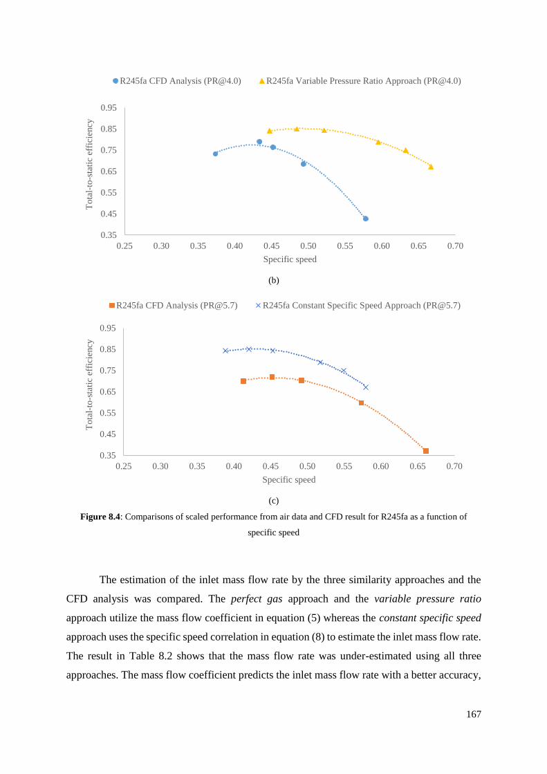
167
(b)
(c)
Figure 8.4: Comparisons of scaled performance from air data and CFD result for R245fa as a function of
specific speed
The estimation of the inlet mass flow rate by the three similarity approaches and the
CFD analysis was compared. The perfect gas approach and the variable pressure ratio
approach utilize the mass flow coefficient in equation (5) whereas the constant specific speed
approach uses the specific speed correlation in equation (8) to estimate the inlet mass flow rate.
The result in Table 8.2 shows that the mass flow rate was under-estimated using all three
approaches. The mass flow coefficient predicts the inlet mass flow rate with a better accuracy,
0.35
0.45
0.55
0.65
0.75
0.85
0.95
0.25 0.30 0.35 0.40 0.45 0.50 0.55 0.60 0.65 0.70
To
tal-
to-s
tati
c ef
fici
ency
Specific speed
R245fa CFD Analysis ([email protected]) R245fa Variable Pressure Ratio Approach ([email protected])
0.35
0.45
0.55
0.65
0.75
0.85
0.95
0.25 0.30 0.35 0.40 0.45 0.50 0.55 0.60 0.65 0.70
To
tal-
to-s
tati
c ef
fici
ency
Specific speed
R245fa CFD Analysis ([email protected]) R245fa Constant Specific Speed Approach ([email protected])

168
with an error less than 10%, as opposed to the specific speed correlation, with error in the range
of 15 and 25%. Hence, the perfect gas approach and the variable pressure ratio approach
provide better estimations in the inlet mass flow, compared to the constant specific speed
approach.
Table 8.2: Numerical error for different scaling analysis approaches
Working
medium
Pressur
e ratio
Optimal
velocity
ratio
Optimal
specific
speed
Maximum
total-to-static
efficiency
Mass flow
rate (kg/s)
Average
Error (%)
Benchmar
k Air 5.7 0.6 0.42 0.85 0.29
Approach
1
R134a 5.7 0.46 0.35 0.85 3.46
Error
(%) 23.3 25.5 11.8 4.6 16.3
R245fa 5.7 0.38 0.29 0.85 3.75
Error
(%) 31.9 35.9 18.4 9.0 23.8
Approach
2
R134a 2.7 0.6 0.37 0.85 3.46
Error
(%) 7.7 9.8 6.6 4.7 7.2
R245fa 4.0 0.6 0.48 0.85 3.75
Error
(%) 2.9 13.5 9.4 9.0 8.7
Approach
3
R134a 5.7 0.6 0.42 0.85 2.99
Error
(%) 0.0 10.6 11.8 17.6 10.0
R245fa 5.7 0.6 0.42 0.85 3.15
Error
(%) 7.5 7.2 18.4 23.5 14.1
CFD
R134a 2.7 0.65 0.41 0.91 3.63
5.7 0.60 0.47 0.76 3.63
R245fa 4.00 0.58 0.42 0.78 4.12
5.7 0.56 0.45 0.72 4.12

169
8.4 Discussion
The discrepancy in the turbine efficiency if a turbine stage is scaled from one operating
condition into another is attributed to the variation in machine Reynolds number and Mach
number. Various Reynolds number corrections were proposed for centrifugal compressors,
such as ASME PTC-10 [17] and the efficiency-deficiency chart by Pampreen [18]. The
machine Reynolds number, however, does not have significant effect on the change in
efficiency in this study as the effects of viscosity and thermal conductivity can be neglected at
high Reynolds number [19]. Reynolds number, Re=ρUD/μ is a function of density, ρ, tip speed,
U, wheel diameter, D, and dynamic viscosity, μ. The dynamic viscosity of the refrigerants is
much smaller, rendering a higher value in the Reynolds number, in the magnitude of 100 x 106,
as opposed to the Reynolds number of steam, air, and water in the magnitude of 1 x 10⁶. The
turbine inlet condition was varied using the CFD analysis to investigate the correlation between
the machine Reynolds number and the turbine performance, as illustrated in Figure 8.5. The
turbine’s performance is fairly consistent in a wide range of Reynolds number, between 10 and
90. Hence, the Reynolds number effect can be neglected in this study.
Figure 8.5: Effect of machine Reynolds number on turbine’s performance using R134a
0.80
0.85
0.90
0 20 40 60 80 100
To
tal-
to-s
tati
c ef
fici
ency
Reynolds number (x 1e6)
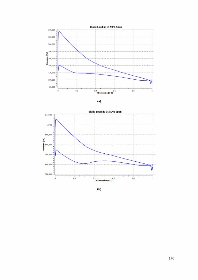
170
(a)
(b)

171
(c)
Figure 8.6: Blade loading and density at blade surface using air at pressure ratio of 5.7 (a), R245fa at pressure
ratio of 4.0 (b) and R134a at pressure ratio of 2.7 (c)
The blade loading along the pressure and suction surfaces at optimal specific speed
using the variable pressure ratio approach are similar for all three working fluids; air, R134a
and R245fa. Constant pressure drop was observed for air (modelled as ideal gas), R134a and
R245fa (modelled as real gas) along pressure surface, but pressure fluctuation was observed
for R245fa along the suction surface. The fluctuation is related to the adverse pressure gradient
near the leading edge of the suction surface, which forms a vortex and local backpressure
downstream of the vortex, as illustrated by the velocity vector in Figure 8.7. The flow re-
attaches downstream of the vortex with gradual pressure drop along the blade passage.
The maximum isentropic efficiency for air, R134a and R245fa is different although the
pressure loading along the blade passage at the optimal specific speed is similar. The highest
turbine efficiency is achieved by R134a, followed by air, and R245fa. The deviation can be
explained as a function of compressibility effect. The compressibility factor is a ratio of actual
specific volume to the ideal volume of selected fluids. The compressibility effect of the
expansion process across the turbine was measured qualitatively by volumetric flow ratio [20].
Macchi and Perdichizzi found that the increase in the volumetric flow ratio gives rise to a
reduction in the turbine efficiency at optimal specific speed [20], and the volumetric flow ratio
has to be less than 50 to achieve a high turbine stage efficiency greater than 0.80 [21]. The
volumetric flow ratio is different for different working fluid using the variable pressure ratio
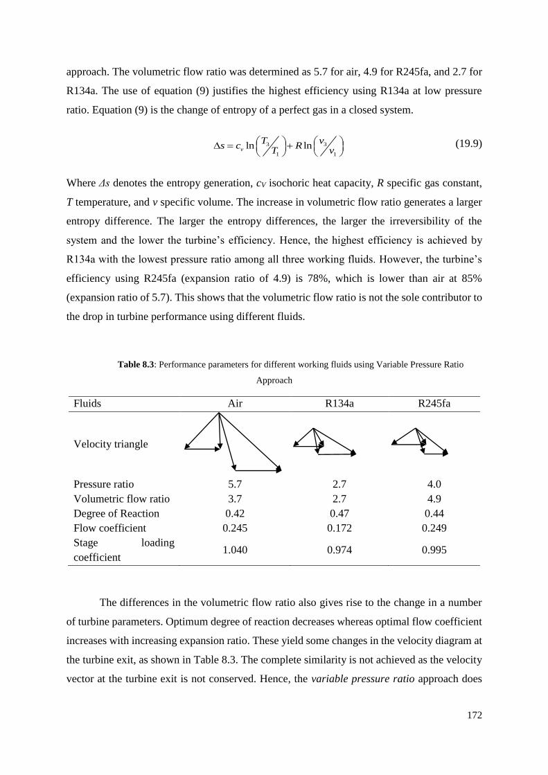
172
approach. The volumetric flow ratio was determined as 5.7 for air, 4.9 for R245fa, and 2.7 for
R134a. The use of equation (9) justifies the highest efficiency using R134a at low pressure
ratio. Equation (9) is the change of entropy of a perfect gas in a closed system.
3 3
1 1
ln lnv
T vs c R
T v
(19.9)
Where Δs denotes the entropy generation, cV isochoric heat capacity, R specific gas constant,
T temperature, and v specific volume. The increase in volumetric flow ratio generates a larger
entropy difference. The larger the entropy differences, the larger the irreversibility of the
system and the lower the turbine’s efficiency. Hence, the highest efficiency is achieved by
R134a with the lowest pressure ratio among all three working fluids. However, the turbine’s
efficiency using R245fa (expansion ratio of 4.9) is 78%, which is lower than air at 85%
(expansion ratio of 5.7). This shows that the volumetric flow ratio is not the sole contributor to
the drop in turbine performance using different fluids.
Table 8.3: Performance parameters for different working fluids using Variable Pressure Ratio
Approach
Fluids Air R134a R245fa
Velocity triangle
Pressure ratio 5.7 2.7 4.0
Volumetric flow ratio 3.7 2.7 4.9
Degree of Reaction 0.42 0.47 0.44
Flow coefficient 0.245 0.172 0.249
Stage loading
coefficient 1.040 0.974 0.995
The differences in the volumetric flow ratio also gives rise to the change in a number
of turbine parameters. Optimum degree of reaction decreases whereas optimal flow coefficient
increases with increasing expansion ratio. These yield some changes in the velocity diagram at
the turbine exit, as shown in Table 8.3. The complete similarity is not achieved as the velocity
vector at the turbine exit is not conserved. Hence, the variable pressure ratio approach does

173
not achieve complete similarity, and this gives rise to the error in estimating the velocity ratio,
specific speed, and turbine performance.
The flow field diagrams of R245fa, R134a, and air using the variable pressure ratio
approach were compared in Figure 8.7. The flow undergoes turning from axial direction to
tangential direction, and gives rise to Coriolis effect in the radial direction [22]. The flow
undergoes a non-uniform velocity distribution in the spanwise direction, with lowest velocity
near the end wall surface of the hub. The radial gradient of the flow velocity in the spanwise
direction gives rise to the imbalance in the pressure gradient in the spanwise direction. The end
result of the Coriolis effect and the non-uniform velocity give rise to a complex flow field,
which is illustrated in Figure 8.7 in term of flow angle. The bulk flow moves from suction
surface near the shroud to pressure surface near the hub. The flow is compensated by a number
of passage vortices, and the flow vector diagram can be found in Kitton’s work (also presented
by Baines in his work [22]). This phenomena exists in the best efficiency point, attributed to
the turning of the flow from axial to tangential direction. The distribution of the swirl angle at
the trailing edge was averaged and the flow angle was determined as 1˚ for air, 33° for R134a
and 37° for R245fa. The result implies that the turbine exit swirl angle might increase
monotonically with the molecular weight of the working fluids, with the highest by R245fa and
the lowest by air. Positive swirl angle is non-favorable as the fluid internal energy would be
lost as kinetic energy. The specific work output would decrease with a positive swirl angle,
based on Euler turbomachinery equation.
2 2 3 3 2 2 2 3 3 3tan tanx m mW U C U C U C U C (19.10)
Where WX is specific work output, U2 is rotor inlet tip speed, U3 is rotor outlet tip speed, Cθ is
tangential velocity component, Cm is meridional velocity component, and α is swirl angle.

174
(a) (b)
(c) (d)
(e) (f)
Figure 8.7: Distribution of relative Mach number in the meridional plane and distribution of absolute flow angle
at the trailing edge using air at pressure ratio of 5.7 (a-b), R245fa at pressure ratio of 4.0 (c-d) and R134a at
pressure ratio of 2.7 (e-f)
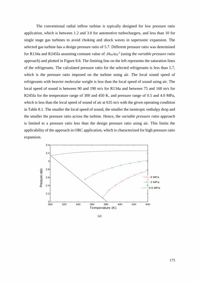
175
The conventional radial inflow turbine is typically designed for low pressure ratio
application, which is between 1.2 and 3.0 for automotive turbochargers, and less than 10 for
single stage gas turbines to avoid choking and shock waves in supersonic expansion. The
selected gas turbine has a design pressure ratio of 5.7. Different pressure ratio was determined
for R134a and R245fa assuming constant value of Δh0s/a012 (using the variable pressure ratio
approach) and plotted in Figure 8.8. The limiting line on the left represents the saturation lines
of the refrigerants. The calculated pressure ratio for the selected refrigerants is less than 5.7,
which is the pressure ratio imposed on the turbine using air. The local sound speed of
refrigerants with heavier molecular weight is less than the local speed of sound using air. The
local speed of sound is between 90 and 190 m/s for R134a and between 75 and 160 m/s for
R245fa for the temperature range of 300 and 450 K, and pressure range of 0.5 and 4.0 MPa,
which is less than the local speed of sound of air at 635 m/s with the given operating condition
in Table 8.1. The smaller the local speed of sound, the smaller the isentropic enthalpy drop and
the smaller the pressure ratio across the turbine. Hence, the variable pressure ratio approach
is limited to a pressure ratio less than the design pressure ratio using air. This limits the
applicability of the approach in ORC application, which is characterized for high pressure ratio
expansion.
(a)
300 320 340 360 380 400 420 4402
2.2
2.4
2.6
2.8
3
3.2
3.4
Temperature (K)
Pre
ssure
ratio
0.5 MPa0.5 MPa
4 MPa4 MPa
2 MPa2 MPa
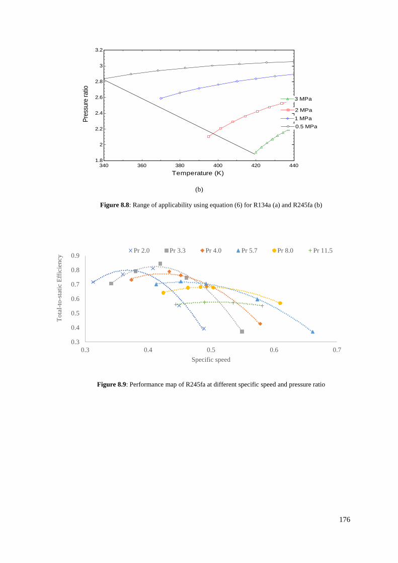
176
(b)
Figure 8.8: Range of applicability using equation (6) for R134a (a) and R245fa (b)
Figure 8.9: Performance map of R245fa at different specific speed and pressure ratio
340 360 380 400 420 4401.8
2
2.2
2.4
2.6
2.8
3
3.2
Temperature (K)
Pre
ssure
ratio
0.5 MPa0.5 MPa
2 MPa2 MPa
3 MPa3 MPa
1 MPa1 MPa
0.3
0.4
0.5
0.6
0.7
0.8
0.9
0.3 0.4 0.5 0.6 0.7
To
tal-
to-s
tati
c E
ffic
iency
Specific speed
Pr 2.0 Pr 3.3 Pr 4.0 Pr 5.7 Pr 8.0 Pr 11.5
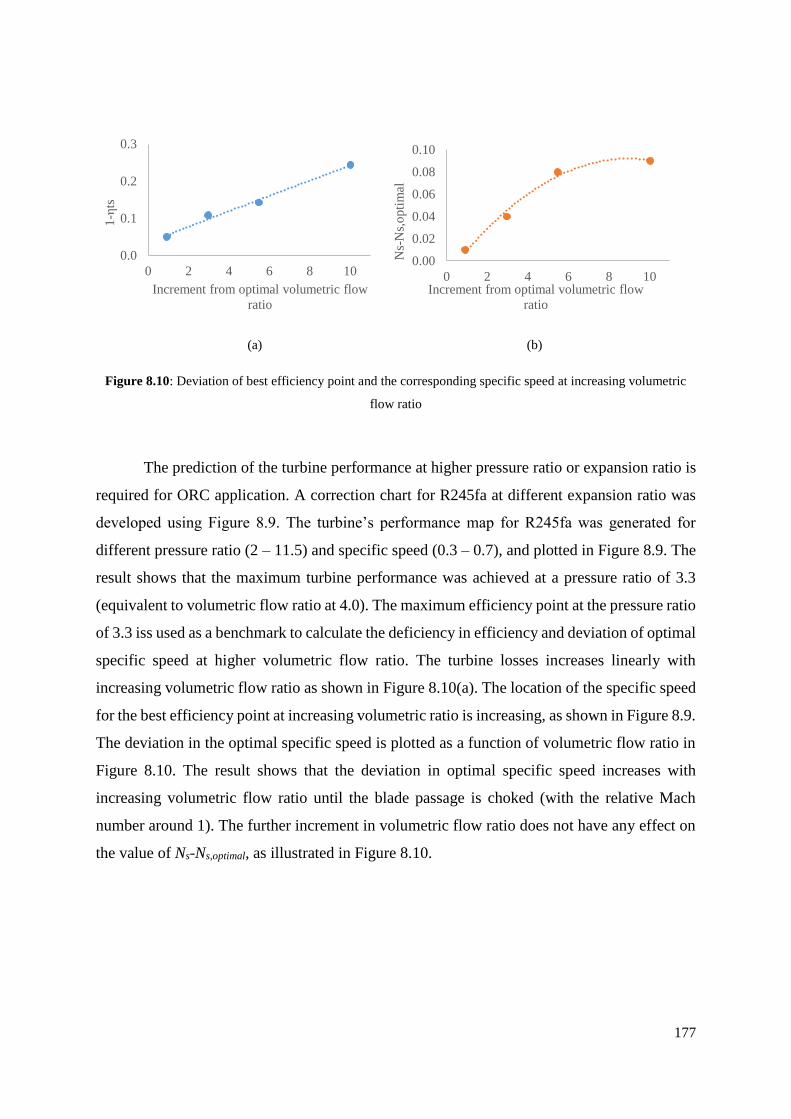
177
(a) (b)
Figure 8.10: Deviation of best efficiency point and the corresponding specific speed at increasing volumetric
flow ratio
The prediction of the turbine performance at higher pressure ratio or expansion ratio is
required for ORC application. A correction chart for R245fa at different expansion ratio was
developed using Figure 8.9. The turbine’s performance map for R245fa was generated for
different pressure ratio (2 – 11.5) and specific speed (0.3 – 0.7), and plotted in Figure 8.9. The
result shows that the maximum turbine performance was achieved at a pressure ratio of 3.3
(equivalent to volumetric flow ratio at 4.0). The maximum efficiency point at the pressure ratio
of 3.3 iss used as a benchmark to calculate the deficiency in efficiency and deviation of optimal
specific speed at higher volumetric flow ratio. The turbine losses increases linearly with
increasing volumetric flow ratio as shown in Figure 8.10(a). The location of the specific speed
for the best efficiency point at increasing volumetric ratio is increasing, as shown in Figure 8.9.
The deviation in the optimal specific speed is plotted as a function of volumetric flow ratio in
Figure 8.10. The result shows that the deviation in optimal specific speed increases with
increasing volumetric flow ratio until the blade passage is choked (with the relative Mach
number around 1). The further increment in volumetric flow ratio does not have any effect on
the value of Ns-Ns,optimal, as illustrated in Figure 8.10.
0.0
0.1
0.2
0.3
0 2 4 6 8 10
1-η
ts
Increment from optimal volumetric flow
ratio
0.00
0.02
0.04
0.06
0.08
0.10
0 2 4 6 8 10
Ns-
Ns,
op
tim
al
Increment from optimal volumetric flow
ratio
178
8.5 Conclusion
Three different approaches using the similarity concept were proposed and investigated
to scale the selected gas turbine from air to R134a and R245fa in this study. The perfect gas
approach assuming the real gas as perfect gas provides the largest error in terms of optimal
velocity ratio, optimal specific speed, and maximum efficiency. The variable pressure ratio
approach shows the highest averaged accuracy in predicting the optimal velocity ratio, optimal
specific speed, maximum efficiency and mass flow rate. The constant specific speed approach
is recommended to estimate the turbine’s performance away from the best efficiency point.
Constant value of Δh0s/a012 was imposed in the variable pressure ratio approach to
achieve the similarity but a number of deviations was observed, including swirl angle at the
turbine outlet, volumetric flow ratio, best efficiency point and the corresponding specific speed.
The Reynolds number effect does not influence the scaling using refrigerants as the effect of
viscosity is negligible at high Reynolds number using refrigerants with low viscosity. The swirl
angle at the turbine outlet was observed as a function of molecular weight, in which the
increment in molecular weight increases the swirl angle and reduces the specific work output.
The variable pressure ratio approach does not ensure a constant volumetric flow ratio, hence
the complete similarity cannot be achieved. The variable pressure ratio approach is limited to
pressure ratio less than the design pressure ratio using air, which is not suitable to scale an ORC
turbine. Therefore, a correction chart was developed to scale the performance of the gas turbine
for higher volumetric ratio using R245fa. The deficiency in turbine efficiency is linearly
correlated to the increased volumetric flow ratio. The correction chart provides a good
estimation in selecting a suitable turbine for a particular ORC application. However, the
correction chart has to be validated against the experimental data for better accuracy.

179
8.6 References
1. Meher-Homji, C.B. ‘The Historical Evolution of Turbomachinery. in Proceedings of
the 29th Turbomachinery Symposium, Texas A&M University, Houston, TX. 2000.
2. Balje, O.E., Turbomachines: A Guide to Design Selection and Theory. 1981: Wiley.
3. Dixon, S.L. and C. Hall, Fluid Mechanics and Thermodynamics of Turbomachinery.
2010, Butterworth-Heinemann: Burlington.
4. Chen, H. and N.C. Baines, The aerodynamic loading of radial and mixed-flow turbines.
International Journal of Mechanical Sciences, 1994. 36(1): p. 63-79.
5. Aungier, R.H., Turbine aerodynamics: axial-flow and radial-inflow turbine design and
analysis. 2006: ASME Press.
6. Japikse, D. and N.C. Baines, Introduction to turbomachinery. 1995: Concepts ETI.
7. Strub, R.A., et al., Influence of the Reynolds Number on the Performance of Centrifugal
Compressors. Journal of Turbomachinery, 1987. 109(4): p. 541-544.
8. Casey, M.V., The Effects of Reynolds Number on the Efficiency of Centrifugal
Compressor Stages. Journal of Engineering for Gas Turbines and Power, 1985. 107(2):
p. 541-548.
9. Quoilin, S. and V. Lemort. Technological and economical survey of Organic Rankine
Cycle systems. in 5th European Conference Economis and Management of Energy in
Industry. 2009. Algarve, Portugal.
10. Bao, J. and L. Zhao, A review of working fluid and expander selections for organic
Rankine cycle. Renewable and Sustainable Energy Reviews, 2013. 24: p. 325-342.
11. Quoilin, S., et al., Thermo-economic optimization of waste heat recovery Organic
Rankine Cycles. Applied Thermal Engineering, 2011. 31(14–15): p. 2885-2893.
12. Sauret, E. Open design of high pressure ratio radial-inflow turbine for academic
validation. in Proceedings of the ASME 2012 International Mechanical Engineering
Congress and Exposition. 2012. Houston, Texas: American Society of Mechanical
Engineers (ASME).
13. Jones, A.C., Design and Test of a Small, High Pressure Ratio Radial Turbine. Journal
of Turbomachinery, 1996. 118(2): p. 362-370.
14. Wong, C.S. and S. Krumdieck. Energy and Exergy Analysis of an Air-Cooled
Geothermal Power Plant with Fixed Nozzle Turbine in Subsonic Expansion and
Supersonic Expansion via CFD Analysis. in 36th New Zealand Geothermal Workshop
2014. Auckland University.
15. Lemmon, E.W., Huber, M.L., McLinden, M.O, NIST Standard Reference Database 23:
Reference Fluid Thermodynamic and Transport Properties-REFPROP, Version 9.1, in
National Institute of Standards and Technology. 2013, Standard Reference Data
Program: Gaithersburg.
16. Lemmon, E.W. and R. Span, Short fundamental equations of state for 20 industrial
fluids. Journal of Chemical & Engineering Data, 2006. 51(3): p. 785-850.
17. PTC, A., PTC 10-1997, Performance test code on compressors and exhausters.
American Society of Mechanical Engineers, New York, 1997. 3.

180
18. Pampreen, R., Small turbomachinery compressor and fan aerodynamics. Journal of
Engineering for Gas Turbines and Power, 1973. 95(3): p. 251-256.
19. Harinck, J., A. Guardone, and P. Colonna, The influence of molecular complexity on
expanding flows of ideal and dense gases. Physics of Fluids (1994-present), 2009.
21(8): p. 086101.
20. Macchi, E. and A. Perdichizzi, Efficiency prediction for axial-flow turbines operating
with nonconventional fluids. ASME Journal of Engineering for Power, 1981. 103: p.
718e24.
21. Angelino, G., C. Invernizzi, and E. Macchi, Organic Working Fluid Optimization for
Space Power Cycles, in Modern Research Topics in Aerospace Propulsion, G.
Angelino, L. De Luca, and W.A. Sirignano, Editors. 1991, Springer New York. p. 297-
326.
22. Moustapha, H., et al., Axial and Radial Turbines. 2003: Concepts Eti.

181
Application of the SMC-DTR
Approaches
9.0 Application of the SMC-
DTR using Meanline Analysis

182
The aim of this thesis is to present the SMC-DTR approach for low temperature
resources, and the main contribution of this thesis is to develop the key component, SMC
adaptive strategy. The following chapters present the application of the SMC-DTR approach
for different resources’ characteristics.
This chapter presents the application of the SMC-DTR approach by adapting nozzle-
less automotive turbochargers for a resource condition with constant heat source and heat sink
condition. The SMC-DTR approach was utilized to design an ORC bottoming cycle in a
petroleum refining plant in New Zealand. The meanline analysis technique was applied as the
performance map of the given turbochargers is not available. The geometry of the turbine
wheels was measured, and the data was fed into the SMC adaptive strategy to evaluate the
turbine performance. The selected automotive turbocharges are not equipped with nozzle
vanes. Hence, a preliminary design of nozzle vanes was performed, and the turbine
performance was evaluated assuming the turbine is equipped with the designed nozzle vanes.
The thermal efficiency of the ORC model was optimized using the two automotive
turbochargers and four different working fluids (n-Pentane, R134a, R245fa, and isobutane).
The selected turbocharger was modified and adapted as an ORC turbine and the mechanical
system design of the ORC turbo-generator set was presented. This chapter aims to present the
SMC-DTR approach using automotive turbochargers as the core test subjects. This chapter
presents the cycle design and fluid selection, the calculation of turbine specification, the SMC
adaptive strategy using meanline analysis technique, and the mechanical system design of the
ORC turbine.
The result shows that the adaptation of the automotive turbochargers as ORC turbine is
feasible but the optimal range of pressure ratio is less than 3.0. If the pressure ratio is above
this value, the turbine performance would drop significantly.
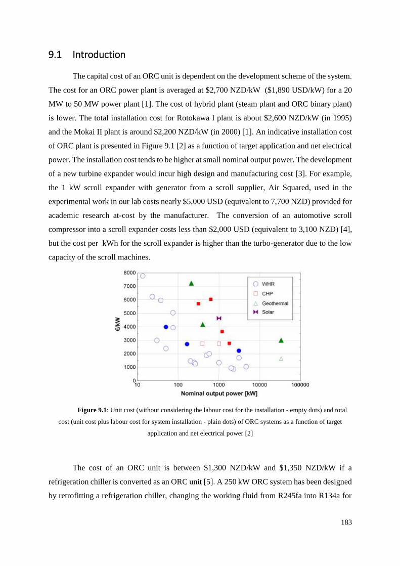
183
9.1 Introduction
The capital cost of an ORC unit is dependent on the development scheme of the system.
The cost for an ORC power plant is averaged at $2,700 NZD/kW ($1,890 USD/kW) for a 20
MW to 50 MW power plant [1]. The cost of hybrid plant (steam plant and ORC binary plant)
is lower. The total installation cost for Rotokawa I plant is about $2,600 NZD/kW (in 1995)
and the Mokai II plant is around $2,200 NZD/kW (in 2000) [1]. An indicative installation cost
of ORC plant is presented in Figure 9.1 [2] as a function of target application and net electrical
power. The installation cost tends to be higher at small nominal output power. The development
of a new turbine expander would incur high design and manufacturing cost [3]. For example,
the 1 kW scroll expander with generator from a scroll supplier, Air Squared, used in the
experimental work in our lab costs nearly $5,000 USD (equivalent to 7,700 NZD) provided for
academic research at-cost by the manufacturer. The conversion of an automotive scroll
compressor into a scroll expander costs less than $2,000 USD (equivalent to 3,100 NZD) [4],
but the cost per kWh for the scroll expander is higher than the turbo-generator due to the low
capacity of the scroll machines.
Figure 9.1: Unit cost (without considering the labour cost for the installation - empty dots) and total
cost (unit cost plus labour cost for system installation - plain dots) of ORC systems as a function of target
application and net electrical power [2]
The cost of an ORC unit is between $1,300 NZD/kW and $1,350 NZD/kW if a
refrigeration chiller is converted as an ORC unit [5]. A 250 kW ORC system has been designed
by retrofitting a refrigeration chiller, changing the working fluid from R245fa into R134a for

184
better thermal match of the heat source and heat sink condition, and replacing the centrifugal
compressor into a radial inflow turbine [5]. The cost of an ORC unit can range from 3,000
€/kW to 7,000 €/kW (correspond to 5,000 and 11,500 NZD/kW) between 100 and 1,000 kW,
based on Figure 5.1. The authors believe that the cost of an ORC unit between 100 and 1,000
kW could be reduced if an existing turbine technology is adapted. An ORC system for waste
heat recovery was developed by converting an automotive turbocharger by ABB Schweiz AG
Switzerland [6]. The conversion process and the cost, however, are not published. The radial
turbines from the automotive turbocharges are believed to be the best candidates for the small-
scale ORC applications due to the high volume manufacturing in a wide range of size at
relatively low cost.
This chapter presents the SMC-DTR approach (shown in Figure 9.2) using automotive
turbochargers as the ORC turbine for a petroleum refining plant in New Zealand. Four different
working fluids were considered, namely n-Pentane, isobutane, R245fa, and R134a. The fluids
were chosen as they are commonly used in commercial ORC units;
R134a in Chena binary plant [7],
Isobutane in Otake pilot plant in Japan [8] and the plant operated by ENEL [9], and
n-Pentane in ORMAT Energy Convertor in Brady [8], and Rotokawa [10].
R245fa was reported as the most suitable candidate in geothermal application with
geothermal brine temperature over 167°C when thermodynamic First-Law efficiency
is the objective function [5].
The performance of two given automotive turbochargers were evaluated using the SMC
adaptive strategy. The meanline analysis technique was applied as the performance map of the
turbine is not available. The thermodynamic cycle was designed based on the heat source and
heat sink condition, the turbine specification was defined, and the turbine performance map
using the four different working fluids was generated. The turbine performance map was fed
into the cycle analysis model to determine the best configuration of turbine and working fluid.
The selected turbine was modified and adapted as an ORC turbine, and the mechanical design
process was presented.

185
Figure 9.2: The SMC-DTR approach for LT-ORC
Heat resource & heat sink
Cycle design & fluid
selection
Selection of vaporizer and
condenser types
Design and development
of heat exchanger
Components testing
System assembly
Field test of power plant
Define turbine
specification
Matching existing
turbines (rotor, or nozzle
and rotor)
SMC Strategy
Mechanical design and
system integration
Laboratory testing
Turbine Adaptation Process

186
9.2 Application of the SMC-DTR approach in a waste heat recovery
(WHR) system
9.2.1 Heat source and heat sink:
An ORC bottoming cycle has been planned for a petroleum refinery plant in New
Zealand [11]. The planned ORC bottoming cycle utilizes the kerosene stream as the heat
source, with the estimated thermodynamic properties of the kerosene flow tabulated in Table
9.1.
Table 9.1: The thermodynamic properties of the kerosene flow [11]
Evaporator Inlet
Evaporator
outlet
Temperature (C) 115 70
Pressure (kPa) 740 740
Enthalpy (kJ/kg) 227.9 134.0
Water has been selected as the cooling medium in the condenser. The cooling water at the
condenser inlet is set at 24˚C and the cooling water is discharged at 35˚C at the condenser
outlet.
9.2.2 Cycle design and fluid selection:
The design and analysis model of the thermodynamic cycle in Chapter 3 was applied
on the heat source and the sink. The turbine efficiency was assumed 85% in the cycle design.
The pinch point temperature different at the evaporator and the condenser were set between 5
and 20˚C to allow a feasible heat transfer within the heat exchangers. Four different working
fluids were selected for the cycle design: n-Pentane, isobutane, R134a and R245fa. The cycle
analysis model was coupled to an optimization code (variable metric method) to optimize the
cycle performance using the overall cycle thermal efficiency as the objective function. The
numerical calculation was performed using Engineering Equation Solver (EES) and the details
of the mathematical model could be found in Chapter 3. The result from the cycle design and
analysis model was tabulated in Table 9.2.

187
Table 9.2: The optimal operating condition of the planned ORC bottoming cycle using four different working
fluids
Fluid - n-Pentane R134a R245fa Isobutane
Inlet total temperature C 74.9 86.2 76.5 78.2
Inlet total pressure kPa 322 2821 724 1294
Outlet static pressure kPa 114 1020 245 523
Total-to-static pressure
ratio - 2.8 2.8 3.0 2.5
Mass flow kg/s 18.5 43.3 36.7 21.2
Cycle thermal efficiency % 7.7 8.2 7.9 8.0
9.2.3 Define turbine specification:
The turbine shaft speed and rotor diameter were determined using the specific speed-
specific diameter performance chart, presented in Chapter 4. The number of stages was
calculated using the flow chart illustrated in Figure 4.3, and the result was presented in Table
9.3.
Table 9.3: The turbine shaft speed, rotor diameter and number of stages for four different working fluids
Fluid - n-Pentane R134a R245fa Isobutane
Specific speed - 0.5 0.5 0.5 0.5
Specific diameter - 4 4 4 4
Shaft speed rev/min 5314 8429 4781 9653
Tip speed m/s 387 277 281 378
Rotor diameter cm 139 62.8 112 74.8
Number of stages - 1 1 1 1
Where station 1 is the nozzle inlet, station 2 is the interface of the nozzle and the rotor, and
station 3 is the rotor outlet in this chapter.

188
9.2.4 Matching existing turbines:
This step was not performed in this case study as there are only two available
automotive turbochargers for the evaluation of the adaptation process. The turbine wheels of
the turbochargers were shown in Figure 9.3.
Figure 9.3: Turbine wheels of two given automotive turbochargers, TC-12 (on the left) and TC-9 (on
the right)
The 12-blade and 9-blade turbine wheels were identified as TC-12 and TC-9 respectively in
this study. The geometry information for the turbochargers was unavailable. Hence the basic
geometry of the turbine wheels was measured manually using a Vernier caliper and a
protractor, and the measurements were shown in Table 9.4. The given turbine wheels are not
similar to the optimal design when the turbine wheels diameter was compared to the result in
Table 9.3. Thus, the following section aims to showcase the application of the DTR-SMC
approach rather than determining the optimal design for the proposed heat resource.

189
Table 9.4: Basic Dimensions Value of Available Turbochargers (TC-9 and TC-12)
Unit TC-9 TC-12
Inlet radius r2 mm 22.3 19.6
Outlet tip radius r3,tip mm 19.3 17.6
Outlet hub radius r3,hub mm 6.5 6.1
Inlet blade height b2 mm 6 6.6
Total blade height btotal mm 18.5 14.2
Blade number Z - 9 12
Inlet blade angle β2,b deg. 0 0
Outlet blade angle at tip β3t,b deg. -55 -70
Outlet blade angle at
hub
β3h,b deg. -45 -50
9.2.5 Design of Nozzle Vanes:
The selected turbine wheels are not equipped with nozzles. A preliminary design of the
nozzle vanes was performed for the selected turbochargers using the method outlined in
Chapter 5. The nozzle vane is designed and set up using the correlations presented by Glassman
[12] and Aungier [13]. The nozzle vane is uncambered and the vane height is constant across
the nozzle stage. The nozzle inlet-to-outlet ratio is recommended to be 1.25 [12]. The nozzle
outlet flow angle was determined using the empirical correlation by Glassman between number
of rotor blades and nozzle outlet flow angle [12], as shown in equation (9.1).
2 2110 tan
30rZ
(20.1)
Where Zr is number of rotor blades, and α2 is the nozzle outlet flow angle. Nozzle inlet flow
angle is usually assumed to be radially inward in the preliminary design stage [14] but this is
not the optimal case. Nozzle inlet flow angle, α1 was calculated using the correlation by
Glassman, shown in equation (9.2), where cs is the chord of nozzle vane, and r3 is the mean
radius at the rotor outlet. The chord of the nozzle vane was calculated using equation (9.3),
which is derived mathematically from the work by Glassman [15]. The equation is only valid
if the vane surface length is equivalent to the chord length, which is applicable for the
uncambered vanes.
2
1
2
2
sintan
cossc
r
(20.2)
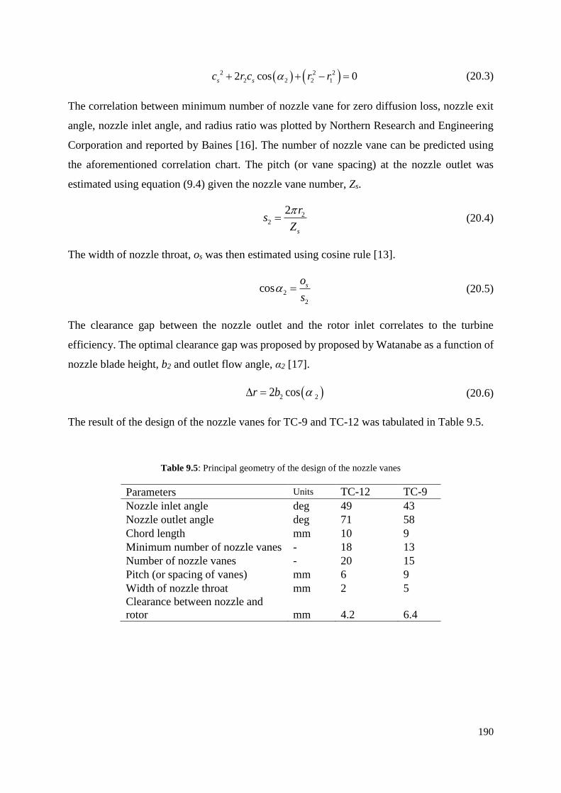
190
2
2 2 2
12 22 cos 0s sc r c r r (20.3)
The correlation between minimum number of nozzle vane for zero diffusion loss, nozzle exit
angle, nozzle inlet angle, and radius ratio was plotted by Northern Research and Engineering
Corporation and reported by Baines [16]. The number of nozzle vane can be predicted using
the aforementioned correlation chart. The pitch (or vane spacing) at the nozzle outlet was
estimated using equation (9.4) given the nozzle vane number, Zs.
22
2
s
rs
Z
(20.4)
The width of nozzle throat, os was then estimated using cosine rule [13].
2
2
cos so
s (20.5)
The clearance gap between the nozzle outlet and the rotor inlet correlates to the turbine
efficiency. The optimal clearance gap was proposed by proposed by Watanabe as a function of
nozzle blade height, b2 and outlet flow angle, α2 [17].
2 22 cos r b (20.6)
The result of the design of the nozzle vanes for TC-9 and TC-12 was tabulated in Table 9.5.
Table 9.5: Principal geometry of the design of the nozzle vanes
Parameters Units TC-12 TC-9
Nozzle inlet angle deg 49 43
Nozzle outlet angle deg 71 58
Chord length mm 10 9
Minimum number of nozzle vanes - 18 13
Number of nozzle vanes - 20 15
Pitch (or spacing of vanes) mm 6 9
Width of nozzle throat mm 2 5
Clearance between nozzle and
rotor mm 4.2 6.4

191
9.2.6 Application of the SMC adaptive strategy
The SMC adaptive strategy was applied to evaluate the performance of the selected
turbine wheels for the ORC bottoming cycle. The meanline analysis technique was applied as
the turbine performance map is not available. The overall calculation flow to evaluate the
performance of the design point (from the cycle design mode) was presented in Figure 9.4. The
calculation flow in Figure 9.5 shows the prediction of the performance at the non-design points
(also known as part-load analysis).
Figure 9.4: Meanline analysis of the turbochargers at optimal velocity ratio
The meanline analysis at the optimal velocity ratio was performed. The turbine
operating condition and the geometry of the designed nozzle vanes and the turbine wheel were
fed into the meanline analysis programme developed in EES. Velocity diagram was constructed
and the thermodynamic properties were determined at each station, where station 1 is the nozzle
inlet, station 2 is the nozzle outlet/rotor inlet, and station 3 is the rotor outlet. The turbine
performance using the selected refrigerants was evaluated using the meanline analysis model
outlined in Chapter 6. The calculated total-to-static isentropic efficiency was compared to the
Define operating
condition &
pressure ratio
Input turbine wheel
geometry
Input the nozzle vane
geometry
Assume ηts and ϕ at
optimal velocity ratio
Construct velocity diagram
Determine thermodynamic
properties at each station
Performance evaluation
using empirical loss model
Calculate ηts
ηts
converges
Proceed to
part load
analysis
No
Yes
update η

192
assumed efficiency. If the error converges to a threshold value (1e-5 in this study), the
numerical calculation proceeds to the next section, part load analysis. If the error does not fall
within the range of the threshold value, the value of the assumed efficiency would be updated
with the calculated value, until the convergence was achieved.
Figure 9.4: Evaluation of turbine performance at part-load operating conditions using meanline analysis
The performance analysis at the part load conditions (at different rotational
speed/velocity ratio) was evaluated using Figure 9.5. The operating condition, and the
geometry of the designed nozzle vanes and the turbine wheel were fed into the meanline
analysis programme. The mass flow rate, ṁ determined from Figure 9.4 was held constant. The
velocity ratio was varied between 0.4 and 1.0. The efficiency was estimated, the velocity
diagram was constructed, and the thermodynamic properties at each station was determined.
The calculated efficiency was compared to the estimated value of the efficiency to check the
convergence. The estimated value would be updated with new value of the efficiency, until the
convergence was achieved. The turbine performance parameters, such as loading coefficient,
and power output, were calculated subsequently.
Use the previous
operating condition
& turbine geometry
Vary the parameter
(pressure ratio/mass
flow)
Construct velocity
diagram
Determine thermodynamic
properties at each station
Performance evaluation
and calculate η
Calculate performance
parameters
Guess-estimate η
ηts
converges?
Yes
No
update η
Hold the velocity ratio
as constant

193
Table 9.6: The performance of TC-9 and TC-12 at the optimal velocity ratio
n-
Pentane R134a R245fa isobutane
TC-9
Velocity ratio - 0.7 0.7 0.7 0.7
Loading coefficient - 0.7 0.7 0.7 0.7
Specific speed - 0.76 0.76 0.76 0.76
Shaft speed rev/min 81,688 59,094 60,173 80,751
Mass flow kg/s 0.18 2.09 0.55 0.72
Power kW 4.7 26.8 7.6 17.7
Isentropic efficiency (total-to-
static) -
0.69 0.66 0.68 0.67
Isentropic efficiency (total-to-
total) - 0.77 0.73 0.76 0.75
TC-12
Velocity ratio - 0.7 0.7 0.7 0.7
Flow coefficient - 0.3 0.3 0.3 0.3
Specific speed - 0.79 0.79 0.79 0.79
Shaft speed rev/min 92,941 67,660 68,462 91,875
Mass flow kg/s 0.15 1.73 0.46 0.60
Power kW 4.6 27.2 7.5 17.5
Isentropic efficiency (total-to-
static) -
0.81 0.80 0.81 0.80
Isentropic efficiency (total-to-
total) - 0.85 0.84 0.85 0.84
The performance of TC-9 and TC-12 at the optimal velocity ratio was presented in
Table 9.6. The optimal velocity ratio was assumed 0.7 for radial section blades [16]. The result
shows that TC-12 is a better candidate for the planned ORC bottoming cycle with higher
isentropic efficiency at 80%, compared to TC-9 with the isentropic efficiency in the range of
66 and 69%. The isentropic efficiency using TC-12 is similar for all four working fluids at the
optimal velocity ratio. R134a was selected attributed to the highest shaft power among the four
working fluids.
A part-load analysis was subsequently performed on TC-12 using R134a as the working
fluid. Two scenario was considered: the first scenario is the mass flow was held constant and
the pressure ratio was varied; the second scenario is the mass flow was varied and the pressure
ratio was held constant.
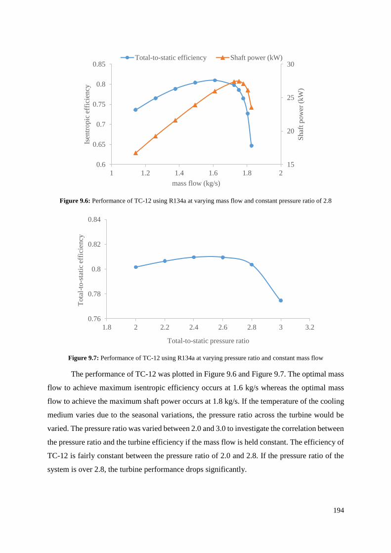
194
Figure 9.6: Performance of TC-12 using R134a at varying mass flow and constant pressure ratio of 2.8
Figure 9.7: Performance of TC-12 using R134a at varying pressure ratio and constant mass flow
The performance of TC-12 was plotted in Figure 9.6 and Figure 9.7. The optimal mass
flow to achieve maximum isentropic efficiency occurs at 1.6 kg/s whereas the optimal mass
flow to achieve the maximum shaft power occurs at 1.8 kg/s. If the temperature of the cooling
medium varies due to the seasonal variations, the pressure ratio across the turbine would be
varied. The pressure ratio was varied between 2.0 and 3.0 to investigate the correlation between
the pressure ratio and the turbine efficiency if the mass flow is held constant. The efficiency of
TC-12 is fairly constant between the pressure ratio of 2.0 and 2.8. If the pressure ratio of the
system is over 2.8, the turbine performance drops significantly.
15
20
25
30
0.6
0.65
0.7
0.75
0.8
0.85
1 1.2 1.4 1.6 1.8 2
Sh
aft
po
wer
(kW
)
Isen
tro
pic
eff
icie
ncy
mass flow (kg/s)
Total-to-static efficiency Shaft power (kW)
0.76
0.78
0.8
0.82
0.84
1.8 2 2.2 2.4 2.6 2.8 3 3.2
Tota
l-to
-sta
tic
effi
cien
cy
Total-to-static pressure ratio
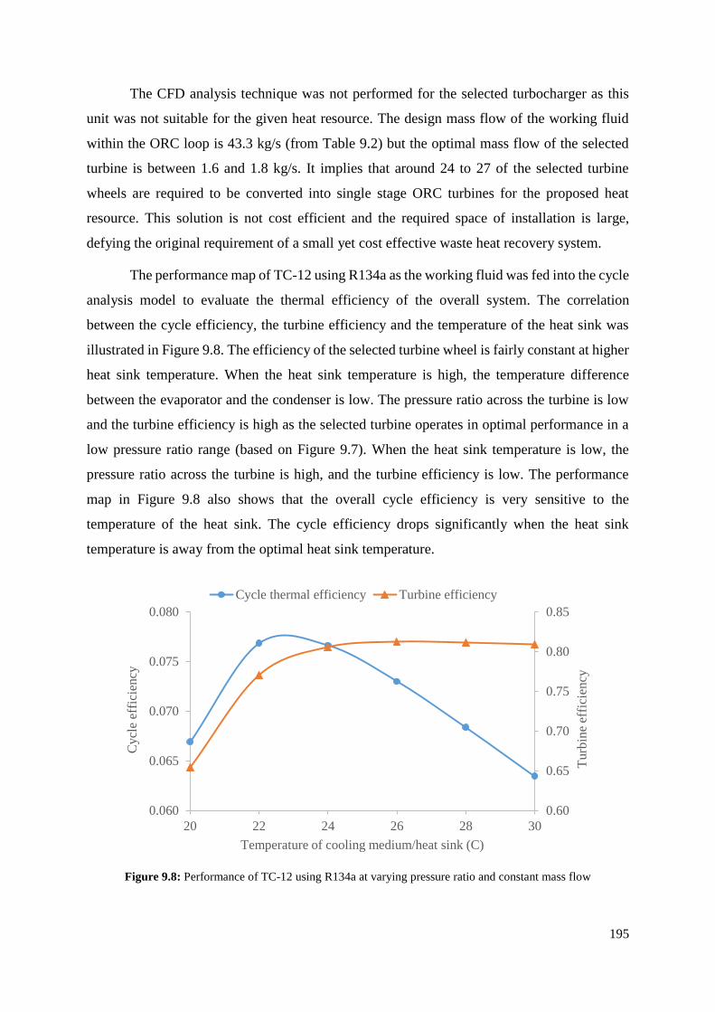
195
The CFD analysis technique was not performed for the selected turbocharger as this
unit was not suitable for the given heat resource. The design mass flow of the working fluid
within the ORC loop is 43.3 kg/s (from Table 9.2) but the optimal mass flow of the selected
turbine is between 1.6 and 1.8 kg/s. It implies that around 24 to 27 of the selected turbine
wheels are required to be converted into single stage ORC turbines for the proposed heat
resource. This solution is not cost efficient and the required space of installation is large,
defying the original requirement of a small yet cost effective waste heat recovery system.
The performance map of TC-12 using R134a as the working fluid was fed into the cycle
analysis model to evaluate the thermal efficiency of the overall system. The correlation
between the cycle efficiency, the turbine efficiency and the temperature of the heat sink was
illustrated in Figure 9.8. The efficiency of the selected turbine wheel is fairly constant at higher
heat sink temperature. When the heat sink temperature is high, the temperature difference
between the evaporator and the condenser is low. The pressure ratio across the turbine is low
and the turbine efficiency is high as the selected turbine operates in optimal performance in a
low pressure ratio range (based on Figure 9.7). When the heat sink temperature is low, the
pressure ratio across the turbine is high, and the turbine efficiency is low. The performance
map in Figure 9.8 also shows that the overall cycle efficiency is very sensitive to the
temperature of the heat sink. The cycle efficiency drops significantly when the heat sink
temperature is away from the optimal heat sink temperature.
Figure 9.8: Performance of TC-12 using R134a at varying pressure ratio and constant mass flow
0.60
0.65
0.70
0.75
0.80
0.85
0.060
0.065
0.070
0.075
0.080
20 22 24 26 28 30
Tu
rbin
e ef
fici
ency
Cycl
e ef
fici
ency
Temperature of cooling medium/heat sink (C)
Cycle thermal efficiency Turbine efficiency

196
9.2.6 Mechanical design and system integration:
TC-12 shows a higher potential turbine efficiency compared to TC-9. The weight of TC-
12 is smaller than TC-9, in which the transient performance of TC-12 is better during the start-
up and shut-down procedure. However, the required rotational speed to achieve optimal
velocity ratio using TC-12 is higher than TC-9 in the range of 4,000 and 11,000 rev/min at the
similar pressure ratio. The objective of this thesis is to demonstrate the application of the SMC-
DTR approach, instead of optimizing the power generation with the particular heat resource.
Hence, a simple prototype design with direct coupling is preferable option to showcase the
design process of the turbo-generator. Hence, TC-9 was selected to demonstrate the mechanical
design and system integration of the SMC-DTR approach.
9.2.6.1 Functional testing
Turbochargers cannot be directly applied into the ORC system due to a number of
issues, which are excessive leakage, poor sealing, unsuitable housing geometry and lubrication
issues. The chosen turbocharger was tested in the research laboratory in University of
Canterbury, as shown in Figure 9.9. The performance of the turbocharger, however, was not
tested due to the constraint of the flow rate of the compressed air of the test facility. The test
aims to investigate the required modification of the turbochargers for ORC application, as the
potential leakage of refrigerants into environment would give rise to health and safety issues
of the plant operators, and the environmental contamination.
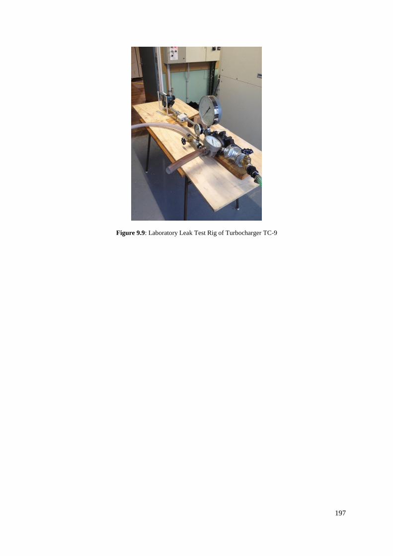
197
Figure 9.9: Laboratory Leak Test Rig of Turbocharger TC-9

198
Leakages
Excessive leakage was found through the turbo gasket which is sandwiched between
the turbine casings. The second major leak site was the bypass valve which is originally used
to limit the pressure ratio across the turbine section and prevent over-speed of the shaft. The
third leak site was along the shaft from the turbine side to the compressor side. Proper seal is
not required in the automotive turbocharger as the exhaust gas could be safely released to the
atmosphere. However, leakage is not tolerated in an ORC system depending on the working
fluids.
Housing Geometry
The chosen turbocharger does not have a nozzle to direct and accelerate the flow into
the turbine wheel, thus reducing the overall turbine efficiency. Hence, a new housing was
designed with stationary vanes to redirect the flow into the turbine rotor.
Lubrication System
Oil-based lubricant was applied to lubricate the bushing and shaft in the selected
turbocharger. This type of lubrication system is not suitable in the ORC turbine due to high
differential pressure between evaporator outlet and condenser inlet. A separate oil pump with
an external oil circuit is required for the ORC turbine. However, the mixture of oil and
refrigerant will reduce the lubricating film thickness on the bearing and shaft which would be
discussed in the following section. The proposed design would use working R245fa as direct
lubrication which was described in the subsequent section.
9.2.6.2 Conceptual Design: Modification of Turbocharger into ORC Turbine
This section discusses the modification required to convert a turbocharger into an ORC
turbine. The laboratory testing of the turbocharger determined the necessary modifications for
the turbine wheel to be adapted, but the casing would need to be re-designed and the bearing
would need to be re-selected. The turbine casing must be re-designed to a fully enclosed model
to avoid leakage through open drive shaft. The turbine shaft would be coupled with a magnetic
coupling which facilitates the coupling with an external high speed generator. O-rings would
be installed between the turbine casings to prevent leakage of high pressure working fluid
through the casing’s gap. The proposed design of an ORC turbine by retrofitting the
turbocharger is shown in Figure 9.10. Modular block design is proposed in the design of a
prototype in order to simplify the manufacturing process.

199
(a) (b)
Figure 9.10: Isometric view and cross-sectional view of proposed design of ORC turbine
Selection of Bearings
Bearings are required to support a rotor shaft in the turbine assembly. The turbine
assembly commonly requires radial bearings and thrust bearings to support both the radial load
and axial thrust. Literature review on steel bearings and hybrid bearings shows that hybrid
bearings are the most suitable bearings for ORC application. In a study by Molyneaux, hybrid
bearings were found to be more suitable than steel bearings in an ORC turbine [18]. The
application of hybrid bearings for refrigerants has also been suggested by Jacobson as the
hybrid bearings have optimal raceway topography to ensure the maximum elastic deformation
of the asperities in Hertzian contact as compared to steel bearings [19]. The optimization of the
raceway allows an effective separation of the mating surfaces, further allowing the bearing to
withstand pure refrigerant lubrication for long periods [19]. The proposed design of the ORC
turbine would be equipped with a pair of hybrid bearings to provide a longer life under
lubrication from pure refrigerants.
Selection of Lubricants
The bearings for steam turbines are usually lubricated by oil lubricants with an external
or separate oil circuit and oil pump [20] whereas the bearings in the ORC application are
lubricated by the working fluid [21]. Two journal bearings and a thrust bearing were lubricated
with R134a in an 18 kW oil-free compressors investigated by Molyneaux [18], and journal
bearings and thrust bearings were lubricated by toluene in a 25 kW solar-powered ORC system
investigated by Nesmith [22]. Common issues in bearing failures by using refrigerants include

200
the attack of bearing surfaces by some refrigerants such as ammonia [19]. Many refrigerants
tend to dissolve into lubricants, such as R134a in ester oil. The mixture reduces the initial
lubricant viscosity and pressure viscosity coefficient thus reducing the film thickness during
lubrication process. Furthermore, the boiling point of the refrigerant-oil mixture is reduced at
the local pressure [23]. The reduction in boiling point allows vaporization of lubricant on the
bearing surface when the bearing surface temperature is higher than the boiling point of the
mixture, thus reducing the lubricant film thickness [19]. The ORC turbine would use the
working fluid as lubricant for the bearings to reduce the cost and complexity of the external
lubrication system.
The rheology of three working fluids, R245fa, R134a and R123 has been studied to
select an optimal lubricant for the bearing. Among the three working fluids, R245fa has been
found as a better lubricant for rolling bearings followed by R134a, and lastly R123 [19].
Though R134a is a relatively poor lubricant compared to R245fa, R134a has been employed
as the lubricant in an oil-free compressor [18] as the pressure viscosity coefficient of R134a is
very similar to the pressure viscosity coefficient of poly alpha olefin oil [19]. The proposed
design of turbo-expander in Figure 9.9 was designed to be lubricated by R134a.
Casing Design and Seal Selection
The turbine casing can be categorized into enclosed and open-drive designs. In an open
drive design, the turbine shaft is coupled to an external generator for power generation. The
working fluid would leak into atmosphere due to high differential pressure between the fluid
inside the turbine and the atmosphere. The most common sealing system for an open drive
design is a dry gas seal and a mechanical seal which are not suitable for small size turbo-
generators. The need for an extra gas buffer system and lubrication system to the seal increases
the cost of the turbo-generator. In a fully enclosed design, the turbine shaft is coupled to a high
speed generator within the enclosed casing. Due to the scarcity of off-the-shelf high speed
generators, the proposed design of ORC turbine would be connected to a magnetic coupling
which facilitates the coupling to an external generator. The casing surrounding the magnetic
coupling would be made from aluminium to allow the operation of magnetic coupling.

201
9.3 Conclusion
This chapter presents the application of the SMC-DTR approach on two nozzle-less
automotive turbochargers, named TC-9 and TC-12 in a planned waste heat recovery (WHR)
system for a petroleum refining plant in New Zealand with constant heat source and heat sink
temperature. The objective of this chapter is to present the SMC-DTR approach. A
thermodynamic cycle of an ORC system was designed for the kerosene flow in the refinery
plant. The SMC turbine adaptive strategy was applied to evaluate the performance of two
turbochargers with four different working fluids (n-Pentane, R134a, R245fa, and isobutane).
The meanline analysis technique was applied as the performance map of the selected turbine
is not available. TC-12 and R134a were determine as the best solution as they show the
maximum turbine efficiency and the shaft power compared to other options. However, the
selected turbocharger was found not cost-effective for the proposed heat resource. Hence, the
CFD analysis in the SMC-DTR approach was not applied. The performance map of TC-12
with R134a was fed into the cycle analysis model to evaluate the correlation between the cycle
performance and the temperature of the cooling medium (or heat sink). Turbocharger cannot
be converted directly as an ORC turbine. Hence, a mechanical concept design was presented
in modifying and adapting the turbocharger as an ORC turbine. This chapter presents the key
steps in the SMC-DTR approach: designing the thermodynamic cycle, evaluating the turbine
performance with different working fluids, optimizing the cycle efficiency with different
turbine options and different working fluids, investigating the performance of the selected
turbine as a function of the heat sink temperature, and the modification and adaption of the
turbocharger into an ORC turbine.
One important lesson from this study is the feasibility of adapting a nozzle-less
automotive turbocharger in an ORC application. However, nozzle has to be designed to direct
the flow into the turbine rotor at an optimal flow angle to yield the optimal turbine performance.
Another lesson is the same turbine wheel can be applied for different working fluid to produce
different amount of work output; TC-12 is expected to produce 4.6 kW using n-Pentane, 27.2
kW using R134a, or 17.5 kW using isobutane. The difference is attributed to the mass flow
into the turbine wheel, which is affected by the specific volume of each working fluid. Lastly,
the performance of the adapted turbocharger is optimal at low pressure ratio less than 3.0. If
the pressure ratio increases, the turbine performance drops significantly.

202
9.4 References
1. Merz, S.K. Assessment of Current Costs of Geothermal Power Generation in New
Zealand (2007 Basis). 2009.
2. Quoilin, S., et al., Techno-economic survey of Organic Rankine Cycle (ORC) systems.
Renewable and Sustainable Energy Reviews, 2013. 22(0): p. 168-186.
3. Qiu, G., H. Liu, and S. Riffat, Expanders for micro-CHP systems with organic Rankine
cycle. Applied Thermal Engineering, 2011. 31(16): p. 3301-3307.
4. Orosz, M., et al., Small Scale Solar ORC system for distributed power. Proc. of the
SolarPaces Conference, 2009.
5. Holdmann, G., The Chena Hot Springs 400kW geothermal power plant: experience
gained during the first year of operation. Chena Geothermal Power Plant Report, Chena
Power Plant, Alaska, 2007: p. 1-9.
6. Buerki, T., et al., Use of a Turbocharger and Waste Heat Conversion System. 2010, EP
Patent 2,092,165.
7. Aneke, M., B. Agnew, and C. Underwood, Performance analysis of the Chena binary
geothermal power plant. Applied Thermal Engineering, 2011. 31(10): p. 1825-1832.
8. DiPippo, R., Second law assessment of binary plants generating power from low-
temperature geothermal fluids. Geothermics, 2004. 33(5): p. 565-586.
9. Ghasemi, H., et al., Modeling and optimization of a binary geothermal power plant.
Energy, 2013. 50(0): p. 412-428.
10. Legmann, H. and P. Sullivan. The 30 MW Rotokawa I geothermal project five years of
operation. in International Geothermal Conference. 2003.
11. Jung, H.C., S. Krumdieck, and T. Vranjes, Feasibility assessment of refinery waste
heat-to-power conversion using an organic Rankine cycle. Energy Conversion and
Management, 2014. 77(0): p. 396-407.
12. Glassman, A.J., Computer program for design analysis of radial-inflow turbines. 1976.
13. Aungier, R.H., Turbine aerodynamics: axial-flow and radial-inflow turbine design and
analysis. 2006: ASME Press.
14. Dixon, S.L. and C. Hall, Fluid Mechanics and Thermodynamics of Turbomachinery.
2010, Butterworth-Heinemann: Burlington.
15. Wasserbauer, C.A. and A.J. Glassman, FORTRAN program for predicting off-design
performance of radial-inflow turbines. NASA Technical Paper, 1975(TN D-8063).
16. Moustapha, H., et al., Axial and Radial Turbines. 2003: Concepts Eti.
17. Watanabe, I., I. Ariga, and T. Mashimo, Effect of dimensional parameters of impellers
on performance characteristics of a radial-inflow turbine. Journal of Engineering for
Power, 1971. 93: p. 81.
18. Molyneaux, A. and R. Zanelli, Externally pressurised and hybrid bearings lubricated
with R134a for oil-free compressors. 1996.
19. Jacobson, B.O. and G.E.M. Espejel, High Pressure Investigation of Refrigerants
HFC245fa, R134a and R123. 2006.

203
20. Couchman, R., K. Robbins, and P. Schofield, GE Steam turbine design philosophy and
technology programs. GE Company, Schenectady, NY, Report No. GER-3705, 1991.
21. David Japikse, F.D.B., Maxwell Hurgin, Keith Patch. Development of a 300 kWe
Integrated Axial Turbine and Generator for ORC Applications. in 2nd Internal Seminar
on ORC Power Systems: Turbo Expanders II. 2013. De Doelen, Rotterdam, The
Netherlands: American Society of Mechanical Engineers (ASME).
22. Nesmith, B., Bearing development program for a 25-kWe solar-powered organic
Rankine-cycle engine. 1985, Jet Propulsion Lab., Pasadena, CA (USA).
23. Yamamoto, Y., S. Gondo, and J. Kim, Solubility of HFC134a in Lubricants and Its
Influence on Tribological Performance. Tribology transactions, 2001. 44(2): p. 209-
214.

204
10.0 Application of the SMC-
DTR using CFD Analysis on
Turbine with Fix Nozzle Vane
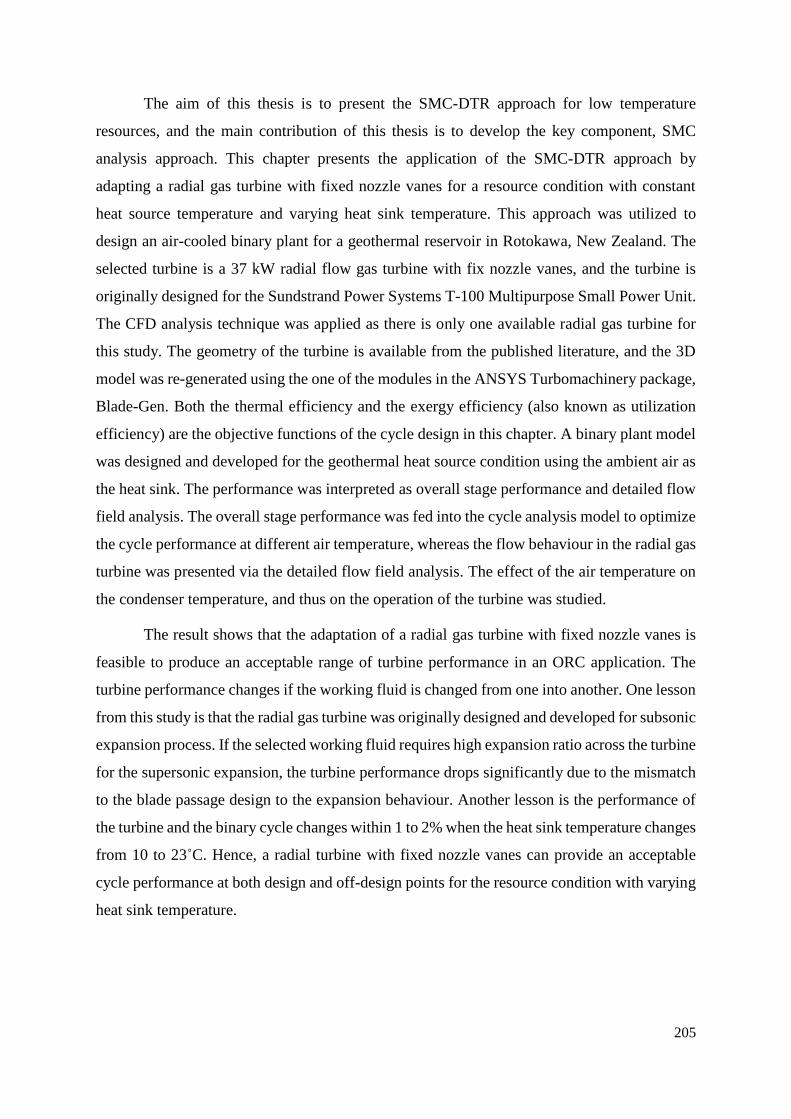
205
The aim of this thesis is to present the SMC-DTR approach for low temperature
resources, and the main contribution of this thesis is to develop the key component, SMC
analysis approach. This chapter presents the application of the SMC-DTR approach by
adapting a radial gas turbine with fixed nozzle vanes for a resource condition with constant
heat source temperature and varying heat sink temperature. This approach was utilized to
design an air-cooled binary plant for a geothermal reservoir in Rotokawa, New Zealand. The
selected turbine is a 37 kW radial flow gas turbine with fix nozzle vanes, and the turbine is
originally designed for the Sundstrand Power Systems T-100 Multipurpose Small Power Unit.
The CFD analysis technique was applied as there is only one available radial gas turbine for
this study. The geometry of the turbine is available from the published literature, and the 3D
model was re-generated using the one of the modules in the ANSYS Turbomachinery package,
Blade-Gen. Both the thermal efficiency and the exergy efficiency (also known as utilization
efficiency) are the objective functions of the cycle design in this chapter. A binary plant model
was designed and developed for the geothermal heat source condition using the ambient air as
the heat sink. The performance was interpreted as overall stage performance and detailed flow
field analysis. The overall stage performance was fed into the cycle analysis model to optimize
the cycle performance at different air temperature, whereas the flow behaviour in the radial gas
turbine was presented via the detailed flow field analysis. The effect of the air temperature on
the condenser temperature, and thus on the operation of the turbine was studied.
The result shows that the adaptation of a radial gas turbine with fixed nozzle vanes is
feasible to produce an acceptable range of turbine performance in an ORC application. The
turbine performance changes if the working fluid is changed from one into another. One lesson
from this study is that the radial gas turbine was originally designed and developed for subsonic
expansion process. If the selected working fluid requires high expansion ratio across the turbine
for the supersonic expansion, the turbine performance drops significantly due to the mismatch
to the blade passage design to the expansion behaviour. Another lesson is the performance of
the turbine and the binary cycle changes within 1 to 2% when the heat sink temperature changes
from 10 to 23˚C. Hence, a radial turbine with fixed nozzle vanes can provide an acceptable
cycle performance at both design and off-design points for the resource condition with varying
heat sink temperature.

206
10.1 Introduction
The turbine technologies suitable for a geothermal binary plant are the multiple stage
axial turbine and the single stage radial inflow turbine. The geothermal binary plant in
Ngatamariki, New Zealand is powered by a two-stage axial turbine whereas the binary plant in
Still Water, Nevada, US, is powered by a single stage radial inflow turbine. The concept of
adapting a gas turbine for binary plant was proposed by the author to reduce the design and
development cost of the turbine for binary plant. This concept facilitates the new entrants to
the ORC market without the decades of engineering development required for new turbine
design. The application of the radial gas turbines into a binary plant provides an alternative
turbine solution, which would assist the development of Organic Rankine cycle (ORC) in
geothermal, waste heat recovery, and biomass applications. However, the application of the
market available gas radial turbines using refrigerants has not been investigated and no relevant
open literature was found.
The application of the radial gas turbines into a binary plant still imposes a number of
questions, including:
Does the turbine stage provide the similar efficiency using the working fluids different
from the original design? And
Is the adapted turbine sensitive to the change in operating condition?
The performance of an air-cooled binary plant is susceptible to the change in ambient
temperature. For example, the net power output of the air-cooled geothermal plant was reduced
by up to 40% from winter to summer in northern Nevada [1]. The change in ambient
temperature affects the pressure ratio and the mass flow across the turbine. A turbine is usually
designed for a set of mass flow rate and pressure ratio. If the pressure ratio and the mass flow
change, the turbine efficiency drops. Hence, an accurate turbine off-design model is crucial in
predicting the performance of an air-cooled binary plant across the life cycle. Several
researchers have investigated the off-design effects of the ORC. The change in ambient
temperature contributes to off-design performance of the turbo-generator. Greg [2] has
modelled the turbine off-design performance as a deviation from the velocity ratio using the
corrections chart from Balje [3]. The turbine correlation chart developed by Balje, however, is
limited to incompressible fluids [3]. The turbine-generator efficiency was assumed to be
constant by Cengel [1] and Marco [4] in modelling the binary geothermal plant. Mitsos
modeled the turbine performance with isobutane as a function of the design isentropic

207
efficiency, ratio of enthalpy drop and ratio of volumetric flow rate [5]. None of the model has
utilized the CFD analysis in modelling an ORC system due to the high computational cost. One
advantage of utilizing the SMC-DTR approach is the performance of the adapted (or selected)
turbine has to be fed back into the cycle model to determine the turbine performance at both
design point and the off-design points. This step allows an engineer or a financial analyst to
predict the earnings and the financial benefits of the design more accurately.
This chapter aims to showcase the application of the SMC-DTR approach (illustrated
in Figure 10.1) by adapting a radial gas turbine with fixed nozzle vanes to design an air-cooled
geothermal binary plant for resources with varying heat sink temperature. The SMC adaptive
strategy was applied to evaluated the turbine performance, and the CFD analysis technique was
applied (based on the criteria selection presented in Figure 10.2) as there is only one available
turbine option in this case study. The turbine performance map was fed into the cycle analysis
model to evaluate the performance of the turbine and the binary cycle at varying heat sink
temperature.

208
Figure 10.1: The SMC-DTR approach for LT-ORC
Heat resource & heat sink
Cycle design & fluid
selection
Selection of vaporizer and
condenser types
Design and development
of heat exchanger
Components testing
System assembly
Field test of power plant
Define turbine
specification
Matching existing
turbines (rotor, or nozzle
and rotor)
SMC Strategy
Mechanical design and
system integration
Laboratory testing
Turbine Adaptation Process

209
Figure 10.2: SMC adaptive strategy
10.2 Application of the SMC-DTR Approach to Design an Air-Cooled
Binary Plant
The SMC-DTR approach was presented to design an air-cooled geothermal binary plant
based on an industrial radial gas turbine. The selected gas turbine was originally designed and
developed for the Sundstrand Power Systems model T-100 Multipurpose Small Power Unit
with nominal power output of 37 kW, with capability up to 75 kW [6]. A binary plant model
was designed using four different working fluids (R134a, R245fa, n-Pentane, and isobutane)
was developed using the heat source and heat sink condition in Rotokawa. The turbine
specification and the matching to the existing turbines were not performed as there is only one
available radial gas turbine with published geometry for use in this study. The performance of
the selected radial gas turbine was evaluated using the SMC adaptive strategy. The
performance curve of the radial turbine using different working fluids was generated. The
performance map of the selected turbine was fed into the cycle analysis model to predict the
overall cycle performance at different ambient temperature. The mechanical design process
was not performed as the process would be very similar to the adaptation process in chapter 9.
Similarity Analysis
Meanline Analysis
CFD Analysis
1
2
3
Mechanical design
Selection of Turbine
η is acceptable?
Yes
No
Cycle design (re-select fluid) or turbine
selection (re-select existing turbines)
1: Turbine performance map (using air as working medium) is available.
2: Turbine performance map is not available.
3: Only one existing turbine is available.

210
10.2.1 Heat source and heat sink
A case study was performed using the Rotokawa geothermal reservoir as the heat source
and the ambient air as the heat sink. The Rotokawa geothermal steam field is one of the largest
geothermal reservoir in use for power generation in New Zealand. Steam power plants and
binary plants have been installed using the Rotokawa geothermal reservoir to produce over 100
MW. The temperature of the geothermal brine of the binary plant was used as the case study
in this chapter. The temperature of the brine fed into the evaporator (also known as vaporizer)
is 217.5°C and the injection well temperature is 150°C [7].
The designed geothermal plant is proposed to have the same cooling mechanism as the
actual binary plant installed in Rotokawa, which is air-cooled condenser. The design ambient
temperature is set at 12°C and the mean temperature across the year was plotted in Figure 10.3.
The distribution of the ambient temperature 11 km from Rotokawa (latitude at -38.68°,
longitude at 176.07°, and height at 385m) was extracted from the climate database [8]. The
temperature includes mean monthly, mean daily maximum, and mean daily minimum air
temperature shown in year 2012. The mean monthly temperature was applied in the binary
plant model in the later section to investigate the binary plant behavior across the year.
Figure 10.3: Average air temperature in Taupo in year 2012
0
5
10
15
20
25
JAN FEB MAR APR MAY JUN JUL AUG SEP OCT NOV DEC
Air
tem
per
ature
(ᵒC
)
Months
Mean Monthly
Mean Daily
Maximum
Mean Daily
Minimum
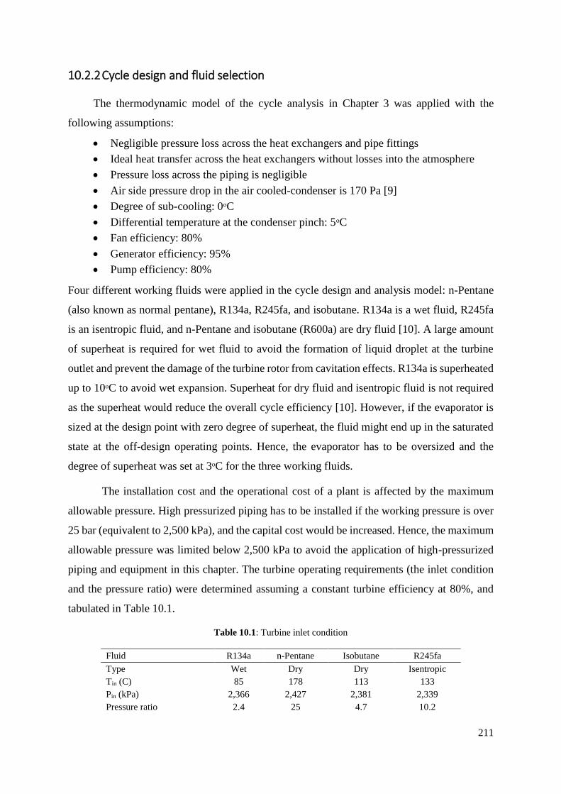
211
10.2.2 Cycle design and fluid selection
The thermodynamic model of the cycle analysis in Chapter 3 was applied with the
following assumptions:
Negligible pressure loss across the heat exchangers and pipe fittings
Ideal heat transfer across the heat exchangers without losses into the atmosphere
Pressure loss across the piping is negligible
Air side pressure drop in the air cooled-condenser is 170 Pa [9]
Degree of sub-cooling: 0ᵒC
Differential temperature at the condenser pinch: 5ᵒC
Fan efficiency: 80%
Generator efficiency: 95%
Pump efficiency: 80%
Four different working fluids were applied in the cycle design and analysis model: n-Pentane
(also known as normal pentane), R134a, R245fa, and isobutane. R134a is a wet fluid, R245fa
is an isentropic fluid, and n-Pentane and isobutane (R600a) are dry fluid [10]. A large amount
of superheat is required for wet fluid to avoid the formation of liquid droplet at the turbine
outlet and prevent the damage of the turbine rotor from cavitation effects. R134a is superheated
up to 10ᵒC to avoid wet expansion. Superheat for dry fluid and isentropic fluid is not required
as the superheat would reduce the overall cycle efficiency [10]. However, if the evaporator is
sized at the design point with zero degree of superheat, the fluid might end up in the saturated
state at the off-design operating points. Hence, the evaporator has to be oversized and the
degree of superheat was set at 3ᵒC for the three working fluids.
The installation cost and the operational cost of a plant is affected by the maximum
allowable pressure. High pressurized piping has to be installed if the working pressure is over
25 bar (equivalent to 2,500 kPa), and the capital cost would be increased. Hence, the maximum
allowable pressure was limited below 2,500 kPa to avoid the application of high-pressurized
piping and equipment in this chapter. The turbine operating requirements (the inlet condition
and the pressure ratio) were determined assuming a constant turbine efficiency at 80%, and
tabulated in Table 10.1.
Table 10.1: Turbine inlet condition
Fluid R134a n-Pentane Isobutane R245fa
Type Wet Dry Dry Isentropic
Tin (C) 85 178 113 133
Pin (kPa) 2,366 2,427 2,381 2,339
Pressure ratio 2.4 25 4.7 10.2

212
Degree of superheat (C) 10 3 3 3
ηcycle 5.9 % 15.4% 10.0 % 12.1%
Nominal Power (kW) 55 kW 300 kW 80 kW 135 kW
There is a significant difference in the predicted plant performance (especially the
potential power output) for the same configuration, the same turbine efficiency, and the same
temperatures attributed solely to the working fluid thermodynamic behavior. The maximum
cycle efficiency was achieved by n-Pentane, in line with the maximum cycle temperature.
However, the required pressure ratio using n-Pentane is too high for the selected radial gas
turbine in a single stage configuration. A multi-stage axial turbine is required to achieve the
required pressure ratio in subsonic expansion process within the turbine passage. Hence, the
CFD analysis was performed using the other three working fluids, R134a, R245fa and
isobutane.
The theoretical maximum thermal efficiency of a thermodynamic cycle is usually
estimated using Carnot efficiency assuming an isothermal heat addition at the heat source
temperature and an isothermal heat rejection at the heat sink temperature. However, the brine
does not serve as an isothermal heat source since the brine temperature decreases during the
heat transfer process. DiPippo has proposed a triangular cycle efficiency with an isobaric heat
addition process to better represent the possible maximum cycle efficiency for the binary plant
[11].
H L
TRI
H L
T T
T T
(21.1)
Where ηTRI is the triangular cycle efficiency (also known as theoretical maximum efficiency of
a binary plant), TH is the heat source temperature, the brine inlet temperature, and TL is the heat
sink temperature, the ambient air temperature. This efficiency serves as a benchmark to the
cycle performance for different working fluids in this chapter.
10.2.3 Define turbine specification:
This step was not performed as this chapter aims to investigate the potential turbine
efficiency and power output of adapting the radial gas turbine for the given heat resource.

213
10.2.4 Matching existing turbines:
This step was not performed since there is only one available radial gas turbine with
published geometry for use in this study. Hence, it is not necessary to select a suitable turbine
from a pool of options using this method.
10.2.5 Application of the SMC Adaptive Strategy
The SMC adaptive strategy was applied to evaluate the performance of the selected
radial gas flow turbine for the air-cooled binary plant. The CFD analysis technique was applied
as there is only one existing turbine available for the given heat source. The gas turbine was
designed and developed originally for air at high speed operation, at 106,588 rev/min with
nominal power of 37 kW. A number of modification is required to adapt the radial gas turbine
into an ORC turbine, including the replacement of the high speed generator to a lower speed
generator, re-design the casing and re-design the mechanical system to contain the refrigerants
from leaking into the atmosphere. This section presents the CFD analysis technique of the SMC
adaptive strategy to evaluate the turbine performance before proceeding to the mechanical
system design. The CFD analysis aims to predict the turbine performance and determine the
optimal turbine operating condition. The process flow of applying the CFD analysis was
presented in Figure 10.4. The detail of the CFD analysis was discussed and presented in
Chapter 7.

214
Figure 10.4: Process flow of applying CFD analysis technique
The CFD analysis technique involves a number of critical steps: generate the 3D model,
mesh the flow domain, set up the boundary condition, solve the Navier-Stokes equations, and
analyze the data. The 3D model of the turbine nozzle and rotor was re-generated using ANSYS
Blade-Gen and the flow domain was meshed using ANSYS Turbo Grid. Steady state analysis
was performed via ANSYS-CFX 14.5 to determine the overall performance of the radial
turbine, as detailed in Chapter 7. Frozen rotor was defined at the interface between the nozzle
and rotor in ANSYS-CFX to take account of the non-axisymmetric flow at the interface. The
model was first validated using air as the working fluid with the published experimental data
[6]. The result of the CFD model agrees with the experimental data with error less than 1% in
the efficiency, and the detail was presented in Chapter 7.
The operation of the gas turbine using other working fluids, refrigerant and hydrocarbon
with heavy molecular weight, requires a lower rotational speed, in which the rotational speed
can be determined at the optimal velocity ratio.
2 2
2is is
U U
C h
(21.2)
CAD
• Generation of solid model using ANSYS-BladeGen
Meshing
• Hexahedral meshes were formed on the fluid zone across the blades.
Modelling the Physics
• Set up the initial operating and boundary conditions
• Select suitable equations of state (EoS) for working medium
Solver
• Solve Navier-Stokes equations in time and 3-D space using k-ɛ turbulence model.
Fluid flow field
• The numerical result was then transformed into velocity vector, temperature and pressure distribution across the blade.

215
Where U2 is the tip speed at the rotor inlet, Cis is the velocity of the fluid if the fluid is expanded
in an ideal nozzle with the equivalent pressure ratio, and ∆his is the isentropic enthalpy drop at
the given pressure ratio. The performance of the turbine is characterized using the thermal
efficiency (thermodynamic First-Law efficiency) and exergy efficiency (thermodynamic
Second-Law efficiency) [11].
01 03
,
01 3,
I turbine
is
h h
h h
(21.3)
Where ηI,turbine is the thermal efficiency of the turbine, h03 and h03 are the total enthalpy
(stagnation enthalpy) at the turbine nozzle inlet and the turbine rotor outlet, and h3,is is the
isentropic enthalpy at the turbine rotor outlet.
01 03,
01 03 0 3 1(s s )II turbine
h h
h h T
(21.4)
Where ηII,turbine is the exergy efficiency of the turbine, T0 is the dead state temperature, where
the dead state temperature of the air-cooled binary plant is the ambient temperature (or dry bulb
temperature of the air), s1 is the entropy at the turbine nozzle inlet and s3 is the entropy at the
turbine rotor outlet.
10.2.5.1 Integration of Fluid Properties from Fluid Database into ANSYS CFX
This section presents the method to develop the real fluid database in ANSYS CFX
using the fluid database by National Institute of Standards and Technology (NIST). ANSYS
CFX version 14.5 has inbuilt fluid properties for R134a but it does not have the fluid properties
for R245fa and isobutane. The fluid information has to be manually set up to allow the
generation of the table of fluid properties during the simulation. The in-built Aungier Redlich
Kwong model would be applied to determine the fluid properties for the selected fluids, R245fa
and isobutane [12].
( )
( )
RT a Tp
v b c v v b
(21.5)
Where p is the pressure, R is the specific gas constant, T is the temperature, v is the specific
volume, a, b, and c are model coefficients. The model coefficients can be calculated using the
equations below.

216
0
n
c
Ta a
T
(21.6)
2 2
0
0.42747 c
c
R Ta
p (21.7)
20.4986 1.1735 0.4754n (21.8)
Where Tc is critical temperature, pc is critical pressure, ω is acentric factor.
0.08664 c
c
RTb
p (21.9)
0 ( )
cc
c c c
RTc b v
p a v v b
(21.10)
Where vc is critical specific volume. The enthalpy and the entropy has to be determined by the
flow solver to evaluate the enthalpy change and the irreversibility effect across the turbine
stage. The enthalpy is determined from the internal energy equation as below.
v
v
dpdu c dT T p dv
dT
(21.11)
h u pv (21.12)
Where cv is isochoric specific heat, u is internal energy, and h is enthalpy of the fluid.
The entropy change is evaluated using integral below, where cp0 is zero pressure ideal gas
specific heat capacity.
0
( , ) ( , ) lnref
ref ref
Tp
ref ref T T
v vrefv T v
cdp p dps T v s T v dv dT R dv
dT T p dT
(21.13)
The zero pressure ideal gas specific heat capacity is expressed as a fourth order polynomial
equation as a function of temperature [13].
0 2 3 4
1 2 3 4 5
pCa a T a T a T a T
R (21.14)
The correlation of Cp0/R and temperature of isobutane and R245fa was plotted in Figure 10.5.
A curve fitting algorithm in Microsoft Excel was applied to determine the values of the
coefficients. The required user’s inputs for the selected fluids, R245fa and isobutane, such as
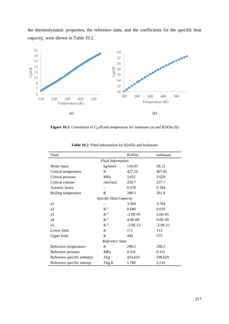
217
the thermodynamic properties, the reference state, and the coefficients for the specific heat
capacity, were shown in Table 10.2.
(a) (b)
Figure 10.5: Correlation of Cp0/R and temperature for isobutane (a) and R245fa (b)
Table 10.2: Fluid information for R245fa and Isobutane
Fluid R245fa isobutane
Fluid Information
Molar mass kg/kmol 134.05 58.12
Critical temperature K 427.16 407.81
Critical pressure MPa 3.651 3.629
Critical volume cm3/mol 259.7 257.7
Acentric factor - 0.378 0.184
Boiling temperature K 288.3 261.4
Specific Heat Capacity
a1 - 3.504 3.764
a2 K-1 0.040 0.019
a3 K-2 -2.0E-05 3.0E-05
a4 K-3 4.0E-09 9.0E-09
a5 K-4 -3.0E-12 -5.0E-11
Lower limit K 171 113
Upper limit K 440 575
Reference State
Reference temperature K 298.2 298.2
Reference pressure MPa 0.101 0.101
Reference specific enthalpy J/kg 424,610 598,029
Reference specific entropy J/kg.K 1,780 2,510
5
7
9
11
13
15
17
19
21
120 220 320 420 520
Cp
0/R
Temperature (K)
10
12
14
16
18
20
22
24
180 280 380 480 580
Cp
0/R
Temperature (K)

218
10.2.5.2 Turbine stage performance
The CFD analysis was performed on the radial turbine for the given operating condition
from Table 10.1. The turbine performance was modeled for each working fluid, except n-
Pentane, at different velocity ratio to determine the optimal rotational speed of the turbine, as
shown in Figure 10.6.
Figure 10.6: Performance analysis of gas turbine using refrigerants at different velocity ratio
The optimal velocity ratio was determined to be in the range of 0.6 and 0.7 from Figure 10.6,
which corresponds to the experimental data of by Jones for the selected gas turbine [6] and the
analytical study by Baines for radial inflow turbines with radial section blades [14]. The
optimal rotational speed of the turbine with the corresponding pressure ratio, and the gear ratio
to couple the turbines to a 60 Hz generator, were presented in Table 10.3.
Table 10.3: Optimal rotational speed of single stage gas turbine with different working fluids
Fluids Pressure Ratio Gear ratio Rotational Speed (rev/min) U/C
R245fa 10.2 8 28,800 0.607
Iso-butane 4.7 11 39,600 0.675
R134a 2.4 6 21,600 0.710
The turbine performance was then simulated at different pressure ratios using the
rotational speed and velocity ratio in Table 10.3, and the turbine performance map was
presented in Figure 10.7. R134a shows a higher total-to-static efficiency, followed by R245fa
and isobutane. A low pressure ratio is preferable for the selected radial turbine for optimal
performance for all three fluids as the turbine was originally designed for subsonic expansion
with low pressure ratio.
0.3
0.4
0.5
0.6
0.7
0.8
0.3 0.4 0.5 0.6 0.7 0.8 0.9 1.0
tota
l-to
-sta
tic
effi
cien
cy
velocity ratio
R245fa isobutane R134a

219
Figure 10.7: Performance analysis of gas turbine as a function of pressure ratio using different working fluids at
optimal velocity ratio
10.2.5.3 Flow Field Analysis
A complete solution of the flow field was generated for the gas turbine using different
fluids, R134a, isobutane and R245fa. R134a and isobutane operating in subsonic expansion
show a higher turbine efficiency than R245fa in supersonic expansion process. The discrepancy
in the efficiency is attributed to the design of the turbine rotor blade passage. The gas turbine
was originally designed for subsonic expansion using air as the working fluid [6]. A minimum
cross-sectional area, known as the throat, exists near the trailing edge of the blade passage. The
throat area determines the flow capacity across the blade passage and allows proper diffusion
of flow at the trailing edge of the blade. Diffusion is required to control the swirl angle of the
flow near the turbine outlet and recover the kinetic energy of the flow, which in turn controls
the specific work output, Wx from the turbine, based on Euler turbomachinery relation.
2 ,2 2 3 ,3 3tan tanx m mW U C U C (21.15)
Where U is the tip speed of the turbine, Cm is the absolute meridional flow velocity, and α is
the absolute flow angle, at the assigned station. Station 2 represents the turbine rotor inlet and
station 3 represents the turbine rotor outlet. The velocity vector of R134a in Figure 10.8 shows
a smooth flow pattern along the blade passage with minimal secondary flow losses. The low
flow velocity at the turbine outlet increases the specific work output of the turbine using the
Euler turbomachinery equation.
0.6
0.7
0.8
0.9
2 3 4 5 6 7 8 9 10 11
To
tal-
to-s
tati
c ef
fici
ency
Total-to-static pressure ratio
R245fa isobutane R134a

220
Figure 10.8: Velocity vector of R134a (on the left) and R245fa (on the right) along the blade passage
The high pressure ratio across the turbine using R245fa produces a supersonic
expansion process in the turbine. The flow accelerates up to the throat along the blade passage,
similar to the subsonic expansion. The flow continues to accelerate downstream of the throat
and the absolute flow velocity increases significantly up to 280 m/s, as shown in Figure 10.8
The over-acceleration of the flow at the downstream of the throat reduces the specific work
output of the turbine stage, based on the Euler turbomachinery equation. The mismatch
between the blade profile and the characteristics of supersonic expansion reduces the turbine
stage efficiency and contributes to the discrepancy of the turbine efficiency between R134a,
isobutane and R245fa.
10.2.5.4 Energy and Exergy Analysis on Turbine and Binary Plant
The turbine performance varies across the year at different ambient temperature, and
the performance across the year was plotted in Figure 10.9. The thermal efficiency and the
exergy efficiency of the turbine using different fluids are fairly constant at different ambient
temperature across the year. R245fa shows the lowest total-to-static efficiency, attributed to
the supersonic expansion across the turbine. It is interesting to note that the turbine using
R245fa shows the highest exergy efficiency although the thermal efficiency is the lowest
among the three fluids. The high exergy efficiency using R245fa is attributed to the lowest
entropy drop during the expansion across the turbine at different pressure ratio, as shown in
Figure 10.10.
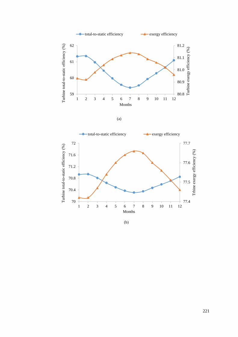
221
(a)
(b)
80.8
80.9
81.0
81.1
81.2
59
60
61
62
1 2 3 4 5 6 7 8 9 10 11 12
Turb
ine
exer
gy e
ffic
iency
(%
)
Turb
ine
tota
l-to
-sta
tic
effi
cien
cy (
%)
Months
total-to-static efficiency exergy efficiency
77.4
77.5
77.6
77.7
70
70.4
70.8
71.2
71.6
72
1 2 3 4 5 6 7 8 9 10 11 12
Trb
ine
exer
gy e
ffic
iency
(%
)
Turb
ine
tota
l-to
-sta
tic
effi
cien
cy (
%)
Months
total-to-static efficiency exergy efficiency
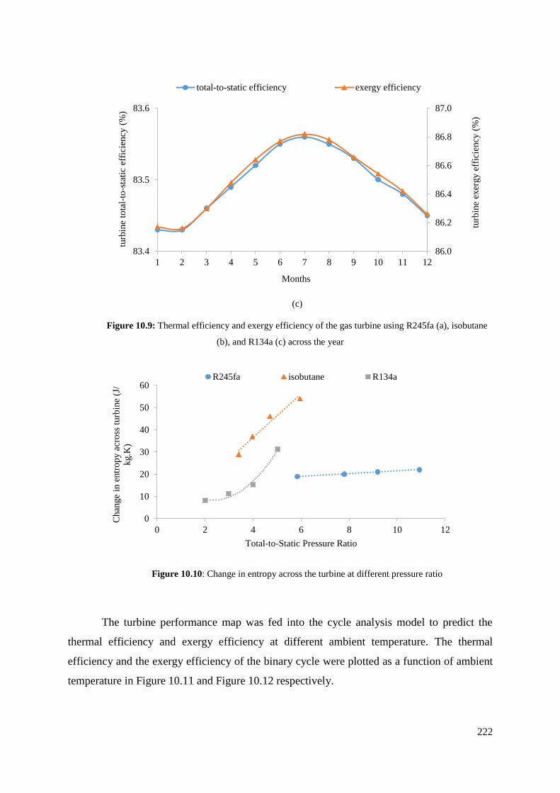
222
(c)
Figure 10.9: Thermal efficiency and exergy efficiency of the gas turbine using R245fa (a), isobutane
(b), and R134a (c) across the year
Figure 10.10: Change in entropy across the turbine at different pressure ratio
The turbine performance map was fed into the cycle analysis model to predict the
thermal efficiency and exergy efficiency at different ambient temperature. The thermal
efficiency and the exergy efficiency of the binary cycle were plotted as a function of ambient
temperature in Figure 10.11 and Figure 10.12 respectively.
86.0
86.2
86.4
86.6
86.8
87.0
83.4
83.5
83.6
1 2 3 4 5 6 7 8 9 10 11 12
turb
ine
exer
gy e
ffic
iency
(%
)
turb
ine
tota
l-to
-sta
tic
effi
cien
cy (
%)
Months
total-to-static efficiency exergy efficiency
0
10
20
30
40
50
60
0 2 4 6 8 10 12
Chan
ge
in e
ntr
op
y a
cro
ss t
urb
ine
(J/
kg.K
)
Total-to-Static Pressure Ratio
R245fa isobutane R134a

223
Figure 10.11: Thermal efficiency of the binary cycle as a function of ambient temperature
Figure 10.12: Exergy efficiency of the binary cycle as a function of ambient temperature
The thermal efficiency of the binary cycle decreases with the rise in ambient
temperature. At higher ambient temperature, the differential temperature between the heat sink
and the heat source is lower, and the cycle thermal efficiency is reduced. However, the thermal
efficiency of the turbine increases with the rise in ambient temperature. The selected radial gas
turbine would perform optimally with higher total-to-static efficiency and lower entropy
change over the summer with lower pressure ratio. The exergy efficiency of the binary plant
increases with respect to the ambient temperature, as the available maximum theoretical work
output from the cycle reduces with increase in ambient temperature, as presented in Figure
10.12. The overall cycle efficiency was compared to the theoretical maximum efficiency of the
binary plant present in Figure 10.13. The cycle thermal efficiency is much lower than the
theoretical maximum efficiency.
5
6
7
8
9
10
6 8 10 12 14 16 18
Cycl
e th
erm
al e
ffic
iency
(%
)
Ambient temperature (C)
R245fa isobutane R134a
8
9
10
11
12
13
6 8 10 12 14 16 18
Exer
gy e
ffic
iency
(%
)
Ambient temperature (C)
R245fa isobutane R134a
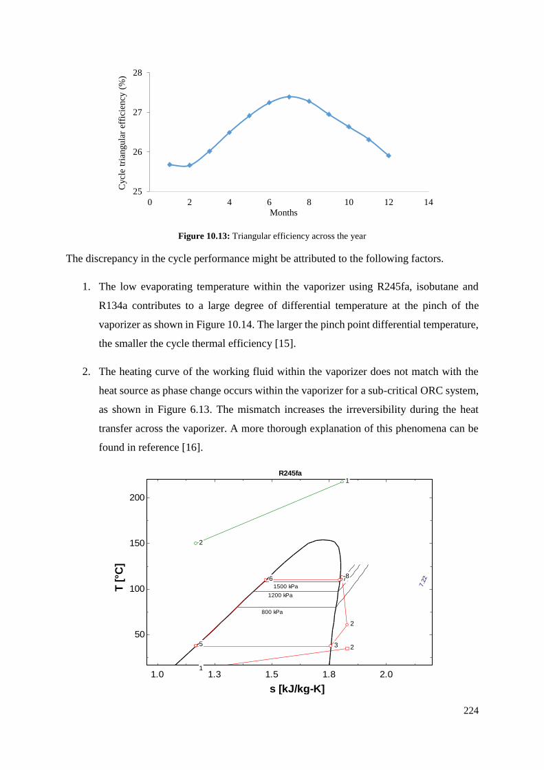
224
Figure 10.13: Triangular efficiency across the year
The discrepancy in the cycle performance might be attributed to the following factors.
1. The low evaporating temperature within the vaporizer using R245fa, isobutane and
R134a contributes to a large degree of differential temperature at the pinch of the
vaporizer as shown in Figure 10.14. The larger the pinch point differential temperature,
the smaller the cycle thermal efficiency [15].
2. The heating curve of the working fluid within the vaporizer does not match with the
heat source as phase change occurs within the vaporizer for a sub-critical ORC system,
as shown in Figure 6.13. The mismatch increases the irreversibility during the heat
transfer across the vaporizer. A more thorough explanation of this phenomena can be
found in reference [16].
25
26
27
28
0 2 4 6 8 10 12 14
Cycl
e tr
iangula
r ef
fici
ency
(%
)
Months
1.0 1.3 1.5 1.8 2.0
50
100
150
200
s [kJ/kg-K]
T [
°C]
1500 kPa
1200 kPa
800 kPa
R245fa
1
2
345
6 78
1
2
1
2
7.2
2

225
Figure 10.14: Simulation of binary plant using R245fa
The exergy efficiency and the thermal efficiency of the binary plant are dependent on
the working fluids and the degree of superheat. Both isobutane and R245fa show a similar trend
of the cycle thermal efficiency and exergy efficiency, with the same degree of superheat despite
the difference in the maximum temperature of the working fluids within the cycle. R134a
shows a similar trend of efficiency as a function of ambient temperature, with the curve shifted
downwards at 2.5% and 3.5% for the thermal efficiency and the exergy efficiency, respectively,
as shown in Figure 10.12. The following correlations were approximated from Figure 10.11
and Figure 10.12 for the cycle thermal efficiency and exergy efficiency as a function of ambient
temperature.
, , ,00.04I cycle amb I cycleT (21.16)
Where ηI,cycle,0 is the cycle thermal efficiency when the ambient temperature is 0ᵒC, and Tamb is
the air ambient temperature for any ACC binary plant, in degree Celsius.
2
, , ,00.0018 0.1II cycle amb amb II cycleT T (21.17)
Where ηII,cycle,0 is the cycle exergy efficiency when the ambient temperature is 0ᵒC. These
equations could be applied to predict the off-design performance of an air-cooled geothermal
binary plant in a preliminary design phase.
10.3 Conclusion
This chapter presents the SMC-DTR approach by adapting a radial gas turbine with
fixed nozzle vanes to design an air-cooled geothermal binary plant for resource condition with
varying heat sink temperature. The CFD analysis technique from the SMC adaptive strategy
was applied as there is only one available turbine option for this case study. This chapter shows
that the adaptation of an existing gas turbine as an ORC turbine is feasible. The rotational speed
of the turbine is much lower when the working fluid is changed from air to refrigerants such as
R134a, R245fa, n-pentane and isobutane. The generator must be modified or replaced to
accommodate the new rotational speed of the turbine.
One of the lessons learned in this chapter is the change in turbine efficiency if the
working fluid is replaced from air into the refrigerants. One of the reasons is attributed to the
original design of the turbine blade passage. The adapted gas turbine was originally designed

226
for sub-sonic expansion process. Hence, the turbine shows a higher isentropic efficiency using
R134a and isobutane in subsonic expansion process and a lower isentropic efficiency using
R245fa in supersonic expansion process.
Another lesson is that the change in the ambient temperature from 10 to 23˚C in
Rotokawa, NZ across the year does not provide any significant effect on the thermal efficiency
and the exergy efficiency of the turbine and the binary cycle. The turbine thermal efficiency
changes up to 2%, and the exergy efficiency up to 1% at the given condition. The efficiency of
the binary cycle changes less than 2% for this temperature range. Hence, the adaptation of a
radial gas turbine with fixed nozzle vanes is suitable to the resource condition with varying
heat sink temperature, with the efficiency changes in less than 2%.

227
10.4 References
1. Kanoglu, M. and Y.A. Cengel, Improving the Performance of an Existing Air-Cooled
Binary Geothermal Power Plant: A Case Study. Journal of Energy Resources
Technology, 1999. 121(3): p. 196-202.
2. Mines, G.L., Evaluation of the impact of off-design operation on an air-cooled binary
power plant. Transactions - Geothermal Resources Council, 2002: p. 701-706.
3. Balje, O.E., Turbomachines: A Guide to Design Selection and Theory. 1981: Wiley.
4. Astolfi, M., et al., Binary ORC (organic Rankine cycles) power plants for the
exploitation of medium–low temperature geothermal sources – Part A: Thermodynamic
optimization. Energy, 2014. 66(0): p. 423-434.
5. Ghasemi, H., et al., Modeling and optimization of a binary geothermal power plant.
Energy, 2013. 50(0): p. 412-428.
6. Jones, A.C., Design and Test of a Small, High Pressure Ratio Radial Turbine. Journal
of Turbomachinery, 1996. 118(2): p. 362-370.
7. Legmann, H. and P. Sullivan. The 30 MW Rotokawa I geothermal project five years of
operation. in International Geothermal Conference. 2003.
8. NIWA, The National Climate Database. 2014: National Institute of Water and
Atmospheric Research.
9. Lukawski, M., Design and optimization of standardized organic Rankine cycle power
plant for European conditions. 2010.
10. Chen, H., D.Y. Goswami, and E.K. Stefanakos, A review of thermodynamic cycles and
working fluids for the conversion of low-grade heat. Renewable and Sustainable Energy
Reviews, 2010. 14(9): p. 3059-3067.
11. DiPippo, R., Geothermal power plants: principles, applications, case studies and
environmental impact. 2012: Butterworth-Heinemann.
12. ANSYS CFX-Solver Theory Guide, Release 14.5. 2012, ANSYS, Inc. Release 14.5:
Canonsburg. p. 372.
13. ANSYS CFX-Solver Modeling Guide, Release 14.5. 2012, ANSYS, Inc: Canonsburg.
14. Moustapha, H., et al., Axial and Radial Turbines. 2003: Concepts Eti.
15. Guo, T., H. Wang, and S. Zhang, Selection of working fluids for a novel low-
temperature geothermally-powered ORC based cogeneration system. Energy
Conversion and Management, 2011.
16. Stijepovic, M.Z., et al., On the role of working fluid properties in Organic Rankine
Cycle performance. Applied Thermal Engineering, 2012. 36: p. 406-413.

228
11.0 Application of the SMC-
DTR using CFD Analysis on
Turbine with Variable Nozzle
Vane

229
The aim of this thesis is to present the SMC-DTR approach for low temperature
resources, and the main contribution of this thesis is to develop the key component, SMC
analysis approach. The objective of this chapter is to utilize the SMC adaptive strategy to
evaluate the performance of an automotive turbocharger with variable nozzle vanes and design
an ORC system for a heat source with fluctuating mass flow.
The first section presents the control strategy to optimize the turbine performance for
varying mass flow using air as working fluid. The CFD analysis technique was applied, and
the performance of the turbine was generated at different velocity ratio, specific speed, mass
flow, and nozzle vane position. The result shows that the inlet mass flow at the turbine inlet is
linearly proportional to the vane angle. The vane angle has to be adjusted to the corresponding
mass flow to optimize the turbine performance.
The second section presents the SMC-DTR approach to design and optimize an ORC
system for a heat source with fluctuating mass flow using the selected turbocharger with the
control strategy from the first section. The cycle design, fluid selection, set up of turbine
specification, matching to the existing turbines, and the mechanical system design were not
performed in this chapter as the previous two chapters have presented the applications of these
steps. This section models the performance of the turbine using air and refrigerants, compares
the turbine performance, and feeds the turbine performance into the cycle analysis model to
evaluate the cycle thermal efficiency for heat sources with varying mass flow. The case studies
in this chapter are the Chena geothermal hot spring in Alaska, USA, and the petroleum refining
plant in New Zealand.

230
11.1 Introduction
The previous two chapters demonstrate the application of the SMC-DTR approach to
design ORC system for low temperature resources, using the off-the-shelf nozzle-less
automotive turbochargers and a radial gas turbine with fix nozzle vanes. The turbines are
adapted assuming that the mass flow of the heat source is constant over the life cycle of the
ORC system. However, this assumption is not applicable in geothermal application. The
productivity of a geothermal well would decline over the time, attributed to the pressure decline
as a result of the fluid extraction from the well [1]. The flow data of 18 wells at The Geysers
steam field in California, USA was analysed by Dykstra [2]. The study shows that there was a
50% reduction in the flow rate extracted from the well after 8 years of the production. Subir
reported that the production rate of The Geysers steam field reduces at 4.8% per year between
1987 and 1995, 2.9% per year between 1998 and 2004, and 2% per year between 2004 and
2011 [3]. The production rate of one of the geothermal wells in Turkey was reported to decline
at nearly 40% per year between year 2012 and 2013 [4]. The flow rate of the brine declined
from 590 tonne/hour to 540 tonne/hour between December 2012 and April 2013. The
application of the radial inflow turbine would provide a low turbine efficiency for the
geothermal resources with declining productivity over the time. The established turbine
performance map (specific speed-specific diameter chart by Balje [5], and specific speed chart
by Dixon [6]) shows that the radial inflow turbine is sensitive to the operating condition. Reza
compared the performance of two radial inflow turbines: one with variable nozzle vanes, and
one with fixed nozzle vanes for a geothermal plant in Nevada, USA. The result shows that the
radial inflow turbine with variable nozzle vanes provides a better efficiency than the turbine
with fixed nozzle vanes at off-design points. Hence, an off-the-shelf turbine with variable
nozzle vanes would be studied to design an ORC system using a heat source with varying mass
flow.
The objective of this chapter is to utilize the SMC-DTR approach to design and
optimize an ORC system for the heat source with varying mass flow, using an automotive
turbocharger with variable nozzle vanes. The first section defines the strategy to optimize the
turbine performance using variable nozzle vanes. The second section models the performance
of the turbine with fixed nozzle vanes and variable nozzle vanes using different working fluids.
The performance of the ORC system using the turbines with fixed nozzle vanes and variable
nozzle vanes was compared. The last part of this chapter investigates the losses within the flow

231
domain across the variable nozzle vanes in order to predict the optimal vane angle for ORC
application.

232
11.2 Test Subject – Automotive Turbocharger with Variable Nozzle
Vanes
The test subject for this chapter is an automotive turbocharger with variable nozzle
vanes (also known as variable nozzle turbocharger and abbreviated as VNT). The smallest
VNT from Garrett Honeywell with an inbuilt ball bearing cartridge was chosen for the study
in this chapter. The model number of the turbocharger is GTB2060VKLR. The variable nozzle
turbocharger by Garrett is classified into different generations, which can be identified from
the model number. GT is the first generation, GTA is the second generation, GTB is the third
generation, and GTC is the optimized version of third generation [7]. Each letter or digit of the
model number gives the information of the type of the system and the geometry of the
components:
20 turbine wheel diameter
60 compressor wheel size
V variable inlet guided vanes
K hydraulically controlled system
L water lubrication
R ball bearing system
This turbine was selected as the turbine equipped with ball bearings requires less amount of
lubrication compared to a turbine equipped with journal bearings. Hence, a VNT equipped with
ball bearings would be a better candidate to be adapted as an ORC turbine. The modification
and adaptation of a turbocharger into an ORC turbine was detailed in Chapter 9.
Figure 11.1: The selected variable nozzle turbocharger from Garrett Honeywell with turbine casing removed

233
11.3 Performance Optimization using Variable Nozzle Vanes
This section aims to investigate the control strategy to optimize the performance of the
automotive turbocharger using variable nozzle vanes. A CFD model (with details outlined in
chapter 7) was applied on the turbine and the performance was predicted at different
parameters: mass flow, velocity ratio, and pressure ratio. The modelling was performed using
air as the working fluid to reduce the computational power and computing time.
One of the challenges in evaluating the performance of the turbochargers for ORC
application is to obtain the 3D model (also known as solid model), which would be imported
into the CFD tools to solve for the potential fluid flow field across the turbines. A number of
approaches are available to obtain the 3D model, including a number of 3D scanning devices,
co-ordinate measurement machines (CMM), and photo-modelling technology. This section use
a portable 3D scanner by Artec to obtain the cloud points and generate the solid model. The
turbine rotor and the nozzle vanes were scanned using a portable 3D scanner from Artec, known
as Artec Spider. A series of linear patterns of blue LED light was projected onto the scanned
object. The distance from the scanner and the object’s surface was determined by the scanner
to obtain the cloud points. The selected 3D scanner is able to capture the details of the scanned
model and textures with an accuracy up to 50 microns, and a resolution up to 100 microns. The
scanned data was processed by the corresponding software, known as Artec Studio, to form the
point cloud using the in-built algorithm. The noise from lighting condition was filtered
manually to avoid the inaccuracy in predicting the object structure. The point cloud was
processed using a parametric solid modelling software, named Geomagic Design X. The point
clouds were connected with tri-angular meshes and the generated surface was smoothened, as
shown in Figure 11.2.
Figure 11.2: Meshed data of the scanned model from Geomagic Design X

234
A 3D model is required to perform the CFD analysis on the turbine. However, the solid
model from the Geomagic Design X cannot be imported directly into ANSYS CFX for the
CFD analysis. A solid model was re-generated in ANSYS Blade-Gen and compared to the solid
model generated from Geomagic Design X. Three solid models were generated at three
different vane positions, namely position 1, position 2, and position 3, as shown in Figure 11.3.
At position 1, the vane was adjusted to a fully open position; at position 2, the vane was adjusted
nearly half of the open position; at position 3, the vane was adjusted to a nearly closed position.
(a) (b) (c)
Figure 11.3: Solid model of the turbine wheel and nozzle generated in ANSYS Blade-Gen, with position 1 (a),
position 2 (b), and position 3 (c)
Meshing was performed in ANSYS Turbo-Grid. O-grids were automated across the
fluid zone, and 116,288 nodes and 104,940 meshes were generated for a single rotor blade,
whereas 167,292 nodes and 154,440 meshes were generated for a single nozzle blade, as
illustrated in Figure 11.4.
The domains, interfaces and boundary conditions of the nozzle and the rotor were set
up in ANSYS CFX. A steady state analysis was selected rather than a transient analysis as the
computational effort would be greatly reduced while providing an accurate result for the overall
turbine stage performance. The interface between the nozzle outlet and the rotor inlet was
defined using the in-built settings – ‘Stage’. The setting averages the interaction effects across
the boundary between the nozzle outlet and the rotor inlet without considering the transient
behavior across the interface. The working fluid, air, was modelled as an ideal gas to reduce
the computing time.
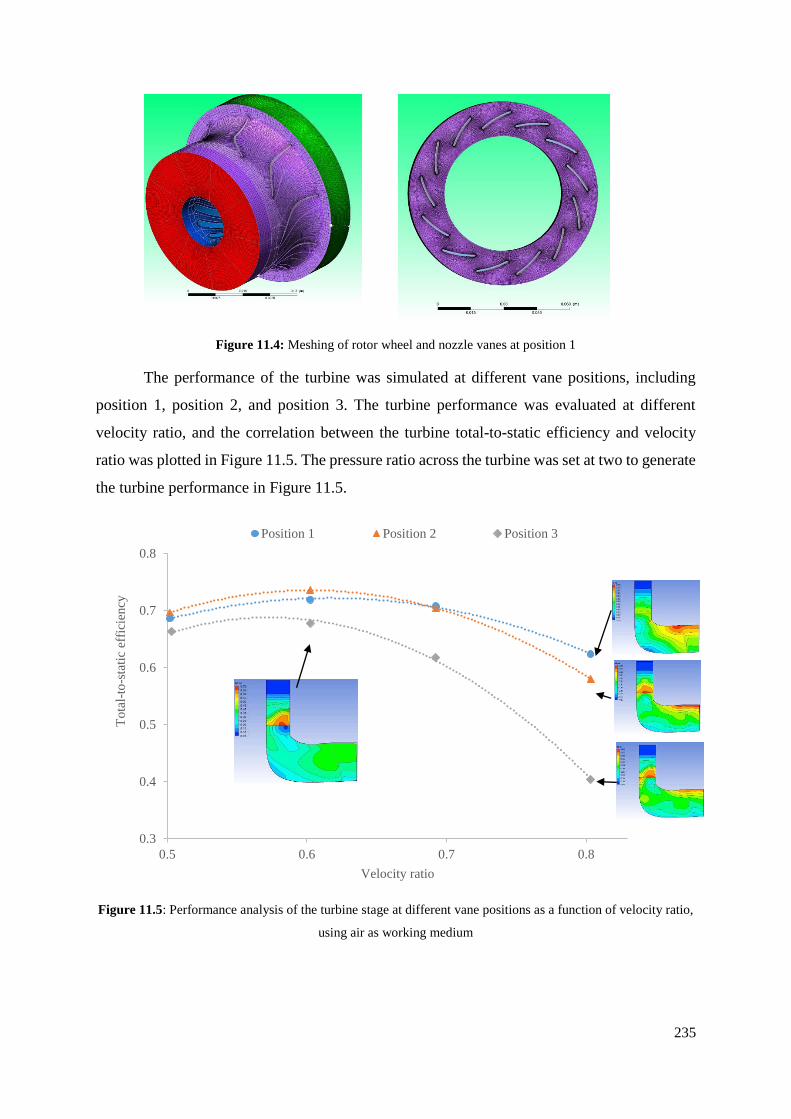
235
Figure 11.4: Meshing of rotor wheel and nozzle vanes at position 1
The performance of the turbine was simulated at different vane positions, including
position 1, position 2, and position 3. The turbine performance was evaluated at different
velocity ratio, and the correlation between the turbine total-to-static efficiency and velocity
ratio was plotted in Figure 11.5. The pressure ratio across the turbine was set at two to generate
the turbine performance in Figure 11.5.
Figure 11.5: Performance analysis of the turbine stage at different vane positions as a function of velocity ratio,
using air as working medium
0.3
0.4
0.5
0.6
0.7
0.8
0.5 0.6 0.7 0.8
To
tal-
to-s
tati
c ef
fici
ency
Velocity ratio
Position 1 Position 2 Position 3

236
The optimal velocity ratio is at 0.6 for all three vane positions, showing that the location of the
optimal velocity ratio is independent of the vane position. The turbine performs at the peak
efficiency when the vane position is set at position 2. The lowest peak efficiency was found
when the vane position is near to the fully closed position (position 3). The contour of
circumferentially area-averaged relative Mach number was included in the performance map
in Figure 11.5. Highest relative Mach number was achieved at the outlet of the nozzle as the
flow was accelerated along the nozzle before entering the rotor. The highest relative Mach
number is well below 1 and choke does not occur at the nozzle outlet. If the relative Mach
number is above 1 at the interface between the nozzle and the rotor, shock wave forms at the
interface, and the fluid potential and kinetic energy would be dissipated as the turbine losses.
Another source of the turbine losses is the secondary flow. The secondary flow effect becomes
significant at high rotational speed (when the velocity ratio is 0.8) and the turbine efficiency
suffers a significant drop due to the secondary flow loss.
Figure 11.6: Performance analysis of the turbine stage at different vane positions as a function of mass flow
The turbine performance analysis was performed at different mass flow rate, and the
correlation between the turbine performance and the mass flow was plotted in Figure 11.6. The
result shows that the turbine performance is sensitive to the inlet mass flow rate, when the
pressure ratio and the vane position is fixed. The turbine efficiency drops significantly if the
0.4
0.5
0.6
0.7
0.8
0.9
0.1 0.12 0.14 0.16 0.18 0.2
To
tal-
to-s
tati
c ef
fici
ency
Mass flow (kg/s)
Position 1 Position 2 Position 3

237
inlet mass flow is different from the optimal mass flow when the vane position is fixed. The
distribution of entropy across the nozzle and rotor blade passage was also included in Figure
11.6, for the maximum efficiency point and the non-optimal operating point. At the non-
optimal operating point, high irreversibility was found at two positions; near the leading edge
of the rotor, and downstream of the trailing edge of the rotor. The phenomena can be explained
as below.
Near the leading edge: Adverse pressure gradient occurs, which gives rise to the flow reversal
and generate vortex flow.
Downstream of trailing edge: The irreversibility is attributed to the mixing of the secondary
flow and the bulk flow across the blade passage, which gives rise to the wake further
downstream from the throat.
The turbine performance was plotted as a function of specific speed in Figure 11.7.
When the vane position was adjusted from position 1 to position 3, the cross sectional area
across the nozzle vane passage was reduced, and the mass flow rate at the turbine inlet was
reduced. The optimal specific speed was reduced from 1.0 at position 1 to 0.7 at position 3.
Figure 11.7: Performance analysis of the turbine stage at different vane positions as a function of specific speed,
using air as working medium
The correlation between the turbine performance, velocity ratio, and pressure ratio was
plotted in Figure 11.8 to determine the optimal velocity ratio at different pressure ratio. The
total-to-static efficiency of the turbine using air was set at pressure ratio of 2 and 4. The contour
of entropy at the highest efficiency point was included in the performance map. The optimal
0.3
0.4
0.5
0.6
0.7
0.8
0.6 0.7 0.8 0.9 1.0 1.1 1.2
To
tal-
to-s
tati
c ef
fici
ency
Specific speed
Position 1 Position 2 Position 3

238
velocity ratio was found at 0.6 for both pressure ratio, indicating that the location of the optimal
velocity ratio is unchanged for different pressure ratio, if the same working medium is applied.
The generation of entropy is higher at higher pressure ratio, especially at the downstream of
the trailing edge of the rotor, which gives rise to lower turbine’s efficiency.
Figure 11.8: Performance analysis of the turbine stage at different pressure ratio using air as working medium,
when the vane was adjusted to position 1 (fully open)
The performance analysis presents the fundamental information to control a variable
nozzle turbine for optimal performance, which are summarized below.
The location of the optimal velocity ratio of a turbine stage is independent of the vane
position and the pressure ratio.
The turbine performance is sensitive to the inlet mass flow rate at different vane
positions.
Hence, the optimal velocity ratio is set by fixing the turbine rotational speed for a given
pressure ratio.
2 2
,
2
60 2s ts is
U r N
C h
(22.1)
0.4
0.5
0.6
0.7
0.8
0.5 0.6 0.7 0.8
To
tal-
to-s
tati
c ef
fici
ency
Velocity ratio
Pr 2 Pr 4

239
Where υ is velocity ratio, U2 is rotor inlet tip speed, Cs is the fluid velocity when the fluid is
expanded in an ideal nozzle with the same pressure ratio of the turbine stage, r2 is radius at the
rotor inlet, and N is turbine shaft speed in rev/min.
An example was showcased using the air as working medium, at total-to-static pressure ratio
of 2. The optimal velocity ratio was found at 0.6 from the performance analysis, and the turbine
shaft speed is adjusted at 87,000 rev/min. The vane position has to be adjusted accordingly to
the inlet mass flow rate; position 1 at 0.19 kg/s, position 2 at 0.13 kg/s, and position 3 at 0.11
kg/s, as shown in Figure 11.6. The vane position could be adjusted either by defining a set of
positions (as shown above), or manipulating the vane angle. The correlation between the mass
flow at the turbine inlet and the vane angle can be approximated by a linear correlation, as
shown in Figure 11.9 using air as the working fluid. The vane position was adjusted
accordingly using the position approach or the vane angle-mass flow correlation in Figure 11.9
for air, to determine the VNT performance. The performance of the VNT and the turbine at the
fixed vanes was simulated using the CFD approach, and compared in Figure 11.10 as a function
of mass flow. The variable nozzle turbine (VNT) shows better efficiency in a wide range of
mass flow rate, between 0.10 and 0.20 kg/s, whereas the turbine performance at fixed vane
position is sensitive to the change in mass flow rate. The application of VNT allows the turbine
to accommodate different mass flow of the working medium, to match with variable demand
in power supply across the day, or to match the variable geothermal heat source condition. The
change in pressure ratio across the turbine stage, however, has to be matched with different
rotational speed, using the velocity ratio parameter for optimal performance.
Figure 11.9: Correlation between inlet mass flow rate of the turbine stage and the vane angle (or absolute flow
angle) at the nozzle outlet
0.10
0.12
0.14
0.16
0.18
0.20
65 66 67 68 69 70 71 72 73 74 75
mas
s fl
ow
(kg/s
)
vane angle/flow angle (deg)

240
Figure 11.10: Comparison of turbine performance using variable nozzle vanes and fixed vanes at position 1
using air as working medium, at pressure ratio of 2
0.60
0.65
0.70
0.75
0.80
0.10 0.12 0.14 0.16 0.18 0.20
To
tal-
to-s
tati
c ef
fici
ency
Mass flow (kg/s)
VNT Fix Vane (Position 1)

241
11.4 Application of the SMC-DTR Approach in Heat Source with Variable
Mass Flow
This section aims to present the application of the SMC-DTR approach to design an
ORC system using a heat source with variable mass flow. The SMC adaptive strategy was
applied to evaluate the turbine performance using refrigerants, compare the turbine
performance using air and using refrigerants, and evaluate the ORC performance by feeding
the turbine performance map into the cycle analysis model.
11.4.1 ORC System
The selected automotive turbocharger was applied on two different case studies; the
geo-fluid from the Chena geothermal hot spring in Alaska [8] and the kerosene flow in a
petroleum refining plant in New Zealand [9]. There are two ORC units installed in the Chena
hot spring producing over 500 kW. An ORC system has been proposed and planned as a
bottoming cycle for the refinery plant. The ORC operating condition was extracted from the
design condition of the binary plant in Chena hot spring [8] and the design condition of a
planned ORC system for the refinery plant [9], as shown in Table 11.1. The planned waste heat
recovery (WHR) system and the binary plant in Chena utilizes R245fa and R134a as the
working fluid respectively. Assumption was made on the mass flow of the heat sources to allow
the study of heat source with variable mass flow in this chapter. The mass flow of the geo-fluid
was assumed to vary from 5 to 10 kg/s, and the mass flow of the kerosene flow was assumed
to vary from 2 to 4 kg/s during the operation.

242
Table 11.1: Resource characteristics and operating parameters of the selected case studies
Application Waste heat recovery Low temperature geothermal
Site Refining NZ, New Zealand Chena Hot spring, Alaska, US
Heat Source
Heat source medium Kerosene flow Hot spring water
Heat source inlet temperature (ᵒC) 115 73.3
Heat source outlet temperature (ᵒC) 70 54.4
Heat sink
Cooling medium Water Water/Air
Cooling medium temperature (ᵒC) 24 4.44
ORC system
Working medium R245fa R134a
Density at turbine outlet (kg/m3) 13.17 20.84
Inlet pressure (kPa) 725 1600
Inlet temperature (ᵒC) 78.6 64.2
Outlet pressure (kPa) 244.7 439
Pressure ratio 3 3.6

243
11.4.2 Application of the SMC Adaptive Strategy
The SMC adaptive strategy was applied to evaluate the performance of the selected
turbocharger for the ORC system with the inlet condition from Table 11.1. The CFD analysis
technique was applied since there is only one turbine option for this chapter. The CFD model
for this turbocharger was presented in the previous section. The total-to-static pressure ratio
was set at 4, since a higher pressure ratio is favorable for ORC application. The correlation
between the turbine performance and the velocity was plotted in Figure 11.11 for vane position
1. A comparison was made on the performance of the selected turbocharger using air and
refrigerants. The result shows that the application of refrigerants in the automotive turbocharger
deteriorates the turbine performance up to 20% in the total-to-static efficiency given the same
pressure ratio. The turbine efficiency was dropped from over 60% to over 40% by replacing
the air with refrigerants as working medium, for the velocity ratio between 0.5 and 0.8. The
location of the optimal velocity ratio was found to shift to a lower velocity ratio, from 0.6 for
air to 0.5 for R134a and R245fa.
Figure 11.11: Comparison of turbine performance for air, R134a and R245fa at pressure ratio of 4, when the
vane was adjusted to position 1 (fully open)
The performance of the VNT using refrigerants was predicted using the control strategy from
the previous section. The correlation between the inlet mass flow and vane angle for R134a
and R245fa was plotted in Figure 11.12. The vane position has to be adjusted accordingly to
the mass flow rate to optimize the VNT performance using R134a and R245fa. The
0.2
0.3
0.4
0.5
0.6
0.7
0.3 0.4 0.5 0.6 0.7 0.8
To
tal-
to-s
tati
c ef
fici
ency
Velocity ratio
R245fa Air R134a

244
performance of the VNT and the turbine at the fixed vane position (at position 1) was compared
in Figure 11.13.
Figure 11.12: Correlation between inlet mass flow and vane angles for R134a and R245fa
(a)
0.0
0.5
1.0
1.5
2.0
2.5
3.0
3.5
66 67 68 69 70 71 72 73 74
mas
s fl
ow
(kg/s
)
vane angle/flow angle (deg)
R134a R245fa
0.2
0.3
0.4
0.5
0.6
0.7
0.8 1 1.2 1.4 1.6
To
tal-
to-s
tati
c ef
fici
ency
mass flow (kg/s)
Fix Vane VNT

245
(b)
Figure 11.13: Comparison of turbine performance between variables nozzle vanes and fixed vanes for R245fa
(a) and R134a (b) at pressure ratio of 4, was a function of mass flow and specific speed
The performance behavior using refrigerants is very similar to the turbine performance
using air. The application of variable nozzle vanes allows the optimized turbine performance
at a wider range of mass flow rate, between 0.8 and 1.6 kg/s for R245fa, and between 1.8 and
3.2 kg/s for R134a. The performance of the turbine using fixed nozzle vanes drops significantly
when the inlet mass flow is deviated from the optimal mass flow. This situation has limited the
application of the radial inflow turbines with fixed nozzle vanes in heat source with
variable/fluctuating mass flow, such as geothermal heat source with decreasing reservoir
pressure/mass flow. The contour plots of the entropy for R134a and R245fa was included in
the performance map. The use of variable nozzle vanes allows a wider range of mass flow
without giving rise to flow separation within the blade passage. Flow separation and flow
reversal occur at non-optimal points if the fixed vane nozzle is used, as shown in Figure 11.13.
The turbine performance was fed into the cycle analysis model, and the cycle
performance using the turbine with fixed nozzle vanes (at vane position 1 – fully open position)
and the turbine with variable nozzle vanes was plotted in Figure 11.14. The result shows that
the ORC system shows a nearly flat efficiency when the turbine with the variable nozzle vanes
was used, despite the significant change of the mass flow of the heat source (2 to 4 kg/s for the
kerosene flow and 5 to 10 kg/s for the geo-fluid). The performance of the overall ORC system
0.3
0.4
0.5
0.6
1.8 2.2 2.6 3 3.4
To
tal-
to-s
tati
c ef
fici
ency
mass flow (kg/s)
Fix Vane VNT

246
would drop significantly if the mass flow of the heat source deviates from the optimal mass
flow. This section successfully shows that the application of variable nozzle vanes in turbine
would maintain the turbine performance and the overall ORC system performance at a wide
range of mass flow of the heat source.
(a)
(b)
Figure 11.14: Comparison of the thermal efficiency of the ORC system between a turbine with fixed nozzle
vanes and a turbine with variable nozzle vanes
0
0.01
0.02
0.03
0.04
0.05
0.06
0.07
0.08
2 2.5 3 3.5 4
Cycl
e th
erm
al e
ffic
iency
mass flow of kerosene flow (kg/s)
R245fa Fix Vane R245fa VNT
0
0.01
0.02
0.03
0.04
0.05
0.06
0.07
0.08
0.09
5 6 7 8 9 10
Cycl
e th
erm
al e
ffic
iency
mass flow of geo-fluid (kg/s)
R134a Fix Vane R134a VNT

247
11.5 Discussion – Performance Evaluation of Variable Nozzle Vanes
This section aims to study the losses in the flow passage of variable nozzle vanes at
different vane positon (or different vane angle). The nozzle loss was quantified as total pressure
loss in this chapter.
01 02
02 2
s
p pK
p p
(22.2)
Where Ks is the total pressure loss coefficient of the nozzle (the subscript s represents the
stator/nozzle), p01 is the stagnation/total pressure at the nozzle inlet, p02 is the total pressure at
the nozzle outlet, and p2 is the static pressure at the nozzle outlet. The correlation between the
nozzle loss coefficients and the velocity ratio of the nozzle vanes using air at different vane
positions was plotted in Figure 11.15.
Figure 11.15: Total pressure loss coefficients of nozzle vanes at different vane position and velocity ratio, using
air as the working medium
The nozzle loss coefficient was found to fall between 0.20 and 0.28 at position 1, between 0.30
and 0.37 at position 2, and between 0.50 and 0.60 at position 3. The nozzle loss coefficient is
fairly constant if the vane position is fixed, and the loss coefficient is not affected by the
velocity ratio of the turbine.
The nozzle loss coefficient with different working fluids was compared in Figure 11.16.
The vane position 1 (fully open position) corresponds to the vane angle at 66˚, the vane position
2 (intermediate position) corresponds to the vane angle at 73˚, and the vane position 3 (nearly
close position) corresponds to the vane angle at 74˚. When the vane angle is low (vane is
0.1
0.2
0.3
0.4
0.5
0.6
0.7
0.5 0.6 0.7 0.8
To
tal
pre
ssure
lo
ss c
oef
fici
ents
(st
ato
r)
Velocity ratio
Position 1 Position 2 Position 3

248
positioned at the fully open position), the loss coefficient is similar despite the type of the
working fluid. When the vane angle is high (vane is positioned at nearly close position), the
loss coefficient with air is higher than the loss coefficient with refrigerants. The nozzle loss
coefficients were found to monotonically increase with increasing vane angle for all three
working fluids. The velocity vector of the fluid flow across the flow domain within the nozzle
vane passage was illustrated in Figure 11.17 to understand the flow behaviour and the source
of the losses.
Figure 11.16: Total pressure loss coefficients of turbine stage with variable nozzles for air, R134a and R245fa
as a function of vane angle
(a) (b) (c)
Figure 11.17: Distribution of velocity and the velocity vector of fluid flow across the nozzle vane at different
vane position using R134a as working fluid; (a) position 1, (b) position 2, and (c) position 3
The distribution of the flow velocity and the velocity vector of the fluid flow across the
flow domain within the vane passage was shown in Figure 11.17 using R134a as the working
0.0
0.1
0.2
0.3
0.4
0.5
0.6
0.7
65 67 69 71 73 75
To
tal
pre
ssure
lo
ss c
oef
fici
ent
(sta
tor)
Vane angle (deg)
Air R245fa R134a

249
fluid, at different vane position. A large circulation zone was observed along the suction surface
of the nozzle vane, for all three vane positions. The larger the vane angle, the larger the
circulation zone, and the larger the nozzle loss coefficients. This phenomena is similar to the
stall of an aircraft. The angle of attack of an aircraft is increased to increase the lift coefficient
during a take-off. The larger the angle of attack, the higher the lift coefficient. However, the
flow separates on the top of the airfoil when the angle of attack is high, creating a large zone
with separated flow and recirculated flow. If the angle of attack is too high, and a threshold
value known as critical angle of attack is exceeded, the separated flow is dominant. The drag
coefficient is dominant and stall occurs. The same explanation can be applied in the variable
nozzle vanes. The increase in the vane angle allows the increase in blade loading across the
nozzle vanes, with a larger pressure ratio across the vanes. The flow, however, separates near
the leading edge of the suction surface, creating a flow circulation zone. The further increase
in the vane angle worsens the separation effect along the suction surface, hence increasing the
nozzle loss coefficients. The increase in the vane angle also limits the throat area and reduces
the allowable volume of the flow across the nozzle vanes. The throat area would be further
reduced attributed to the separation zone formed along the suction surface. The flow fluid in
Figure 11.17 also shows a strong circulation flow at the trailing edge of the vanes, especially
at the vane position 3 (near to the close position). The circulation flow at the trailing edge
would mix with the downstream flow near the rotor inlet, hence contributing to the mixing loss
or passage loss of the flow across the rotor.
Figure 11.18: Performance of turbine with variable nozzle vanes as a function of vane angle, for R134a and
R245fa
0.40
0.45
0.50
0.55
0.60
0.65
66 68 70 72 74 76
To
tal-
to-s
tati
c ef
fici
ency
Vane angle (deg)
R245fa R134a

250
The performance of the turbine with variable nozzle vanes was plotted in Figure 11.18
to showcase the correlation between the turbine performance and the vane angle. Even though
the nozzle loss coefficient increases with the vane angle attributed to the formation of a larger
flow recirculation zone, the turbine provides the highest efficiency at a specific vane angle
between the fully open and fully close vane position. The optimal point can be determined
mathematically once the turbine performance map was generated using the CFD analysis
approach.

251
11.6 Conclusion
The objective of this chapter is to present the SMC-DTR approach to design and
optimize an ORC system for a heat source with fluctuating mass flow by using an automotive
turbocharger with variable nozzle vanes.
The first section presents the control strategy to optimize the performance of the
selected automotive turbocharger using air as the working fluid. The turbine rotational speed
has to be defined using the optimal velocity ratio and the system pressure ratio. The nozzle
vane angle has to be adjusted as a function of the mass flow of the ORC working fluids (or the
mass flow of the heat source) during the operation to maintain the optimal performance of the
turbine.
The second section compares the performance of the turbine and the ORC system
between the turbine with fixed vane position and the turbine with variable nozzle vanes. The
findings are summarized below:
1. The performance of the selected automotive turbocharger deteriorates up to 20% if the
working fluid was changed from air into R134a or R245fa.
2. If the same turbine rotor is used, the use of the variable nozzle vanes provides a better
efficiency for a wider range of mass flow, compared to the use of the fixed nozzle vanes.
3. The thermal efficiency of the ORC with VNT remains between 50 and 70% even if the
mass flow varies from 2 to 3.5 kg/s for the kerosene flow. The thermal efficiency of the
ORC with the turbine with fixed nozzle vanes changes from 50% to 20% when the mass
flow varies from 3.5 to 2.5 kg/s. Hence, the thermal efficiency of the ORC with VNT
provides a better efficiency to match with the heat source with varying mass flow.
4. The nozzle loss coefficient is not affected by the velocity ratio. The loss coefficient
increases when the vane angle is increased. However, an optimal vane angle exists
between the fully open and fully close vane position for maximum efficiency of the
turbine stage. If an existing turbine (or off-the shelf turbine) is used, the optimal vane
angle can be determined using the CFD analysis, as outlined in this chapter.
The result of this chapter provides the valuable information into the SMC-DTR approach that
a turbine with variable nozzle vanes has to be selected if the heat source shows varying mass
flow across the proposed life cycle of the planned power plant.

252
11.7 References
1. Ripperda, M. and G. Bodvarsson, Decline curve analysis of production data from The
Geysers geothermal field. 1987: Lawrence Berkeley Lab.
2. Thomas, R.P., et al., A reservoir assessment of The Geysers geothermal field. 1981,
Californina Department of Conservation, Division of Oil and Gas.
3. Sanyal, S.K. and S.L. Enedy. Fifty years of power generation at the Geysers geothermal
field, California–the lessons learned. in 36th workshop on geothermal reservoir
engineering, Stanford, California. 2011.
4. KARADAS, M., U. SERPEN, and N. AKSOY, Some Investigations on Decline in
Dora-1 Brine Flow Rate, Case Study: AS-1 Production Well.
5. Balje, O.E., Turbomachines: A Guide to Design Selection and Theory. 1981: Wiley.
6. Dixon, S.L. and C. Hall, Fluid Mechanics and Thermodynamics of Turbomachinery.
2010, Butterworth-Heinemann: Burlington.
7. Garrett Performance Turbochargers. [cited 2015 27th May]; Available from:
http://www.turbobygarrett.com/turbobygarrett/turbochargers.
8. Aneke, M., B. Agnew, and C. Underwood, Performance analysis of the Chena binary
geothermal power plant. Applied Thermal Engineering, 2011. 31(10): p. 1825-1832.
9. Jung, H.C., S. Krumdieck, and T. Vranjes, Feasibility assessment of refinery waste
heat-to-power conversion using an organic Rankine cycle. Energy Conversion and
Management, 2014. 77(0): p. 396-407.

253
12.0 Conclusion

254
12.1 Summary
This thesis presents the strategy to design and optimize an ORC system for low
temperature resources by adapting the off-the-shelf radial inflow turbines, named SMC-DTR
approach. This strategy is of primary importance in developing a cost-effective energy
conversion system without having the knowledge-based engineering (KBE) in turbine
technology. The motivation of this research work stems from the limited available research
funding in the development of the KBE in turbine technology for the ORC turbine design. To
this purpose, this thesis addresses the research question of how the energy conversion system
is designed using the off-the-shelf turbines for the working fluid different from the original
design. This thesis work is divided into four major sections, each serving different contribution
to develop, validate, and apply the SMC-DTR approach.
12.1.1 Background
The first section presents the background of the ORC system and the fundamental
modelling of the DTR approach.
Conclusions:
The literature review provides the information of the major parameters for use in the
SMC-DTR approach: the type of turbine. The radial inflow turbine is selected to be adapted in
the SMC-DTR approach. The radial inflow turbine is a better candidate of turbine option for
low temperature resources, as compared to other turbine options, such as axial turbines, and
positive displacement machines for the following reasons:
The radial inflow turbine operates optimally in the pressure range suitable for the low
temperature resources.
The radial inflow turbine can be up-scaled to produce a few megawatts shaft power or
down-scaled to produce as little as a few kilowatts shaft power.
The radial inflow turbine is commercially available in different diameter and in large
volume as automotive turbochargers and gas turbines.
The radial inflow turbine is cheaper to be sourced from the automotive turbochargers,
compared to axial turbine from steam turbines.

255
Secondly, the thermodynamic model of an ORC system, and the method to define the
turbine specification were presented as part of the SMC-DTR approach. The inclusion of these
information is important if the SMC-DTR approach has to be performed or repeated.
12.1.2 Investigative Study
This part presents the turbine preliminary design method coupled with the real gas
model to match the existing turbines to the heat source.
Conclusions:
The selected gas model affects the turbine design outcome during a turbine preliminary
design process. The ideal gas model under-estimate the turbine diameter up to 50% and over-
estimate the turbine shaft speed up to 550%, depending on the compressibility factor of the
working fluid at the turbine inlet. The design outcome using the ideal gas model provides a
poor choice of turbine geometry and turbine operating condition, which might lead to a power
consuming operation (behaving as a pump) instead of a power generation process (operating
as a turbine). Hence, the real gas model has to be coupled into the turbine preliminary design
process to provide an optimal configuration of turbine geometry and operating condition.
Implications:
This section emphasizes the disadvantage of using the conventional turbine preliminary
design approach with ideal gas model for refrigerants and real gases, and presents the numerical
flow process that can be imitated by ORC turbine manufacturers to perform the turbine
preliminary design process using the real gas model.
12.1.3 Components of the SMC Adaptive Strategy
This section develops the analysis techniques of the SMC adaptive strategy: similarity
approach, meanline analysis, and CFD method.
Conclusions:
The similarity analysis approach utilizes the similarity concept to scale a turbine from
one working fluid into different working fluid. Different parameter sets were established and
validated against the CFD model to determine the best parameter set to scale the radial inflow
turbine. The variable pressure ratio approach is proposed at the best efficiency point, and the

256
constant specific speed method is used at the operating points away from the best efficiency
point. A turbine correction chart was developed to scale the turbine for different volumetric
flow rate at the best efficiency point.
The meanline analysis technique is developed using the empirical loss model. The
meanline analysis model consists of five different losses: passage loss, secondary flow loss,
incidence loss, clearance loss, and windage loss. Each loss model has been validated against
the experimental data of the radial turbines using air as working fluid. The empirical loss model
of the meanline analysis was validated against two turbines: an industrial radial gas turbine
using air as working fluid, and a research prototype unit of ORC turbo-generator using R245fa
as working fluid. The meanline analysis is applied when the performance map of the turbine is
not available.
The CFD method provides the most accurate result of the turbine performance
compared to other modelling approaches. The CFD analysis method consists of five main steps:
generate 3D model, mesh the flow domain, set up the boundary condition and select the
turbulence model, solve the Navier-Stokes equation, and analyse the flow field. The CFD
model was developed and validated against the experimental data of an industrial radial gas
turbine using air as working fluid.
Implications:
The three proposed methods (similarity, meanline, and CFD) provide the analytical
tools to analyse the turbine performance at different level of accuracy and computational effort.
These methods were integrated into the SMC adaptive strategy to analyse the turbine
performance using working fluid different from the original design.
The similarity analysis allows the engineer to conduct a preliminary evaluation of the
turbine performance for different working fluid (which cannot be performed prior to this study)
given the performance map of the turbine using air as working fluid. This analysis approach
allows the experimental evaluation of the turbine performance using a compressed air test
bench. The compressed air test bench is simple with low level of hazard, and low installation
and operation cost compared to a full scale turbine test facility using refrigerants as the working
fluids. The turbine can be scaled from air to refrigerants using the similarity analysis approach.
This approach also allows a preliminary screening of the suitability of the off-the-shelf turbines
to be retrofitted or adapted for application with different working fluids.

257
The proposed meanline analysis can be useful in predicting the turbine performance for
ORC application as the model was validated against the experimental data of the ORC turbine.
This analysis model is useful when the information of the turbine, such as the model number
and the performance map, is not available. This approach is simple without the need of a
comprehensive measurement on the turbine.
The proposed CFD model serves as a guideline to analyse and validate radial turbine
performance. The mesh setting in the model can be used for different radial turbine to produce
good, if not best, quality of meshes across the flow domain. This model was refined by the
author to produce the accurate estimation of the turbine performance with the minimal amount
of computational power and computing time.
12.1.4 Application of the SMC-DTR Approaches
This section presents the application of the SMC-DTR approach using three different
turbine technologies; a nozzle-less automotive turbocharger, a fixed vane radial gas turbine,
and an automotive turbocharger with variable nozzle vanes, named variable nozzle
turbocharger (VNT).
Conclusions:
The adaptation of the off-the-shelf radial turbines to design an ORC system is feasible,
with the trade-off of the turbine efficiency. The automotive turbocharger is typically designed
for the pressure ratio between 1.0 and 3.0, whereas the industrial radial gas turbine is designed
for a higher range of pressure ratio, between 3.0 and 5.0. The turbine efficiency deteriorates up
to 20% when the working fluid of the automotive turbocharger is replaced from air into the real
gases or refrigerants. The efficiency of the industrial radial gas turbine changes within the range
of 10% when the working fluid is changed from air into refrigerants. The automotive
turbochargers and the gas turbines are mostly designed for sub-sonic expansion with the
pressure ratio barely goes beyond 5.0. Hence, the application of these turbines in ORC has to
be handled with care to ensure that the expansion process is within the range of sub-sonic
expansion. A supersonic expansion on these turbine leads to low turbine efficiency. For
example, the industrial radial gas turbine in this thesis shows the highest efficiency when the
pressure ratio is between 3.0 and 4.0, and shows the deterioration in efficiency between 20 to
30% at the pressure ratio between 6.0 and 10.0. The rotor flow passage is designed to allow
flow diffusion downstream of the throat, to control the swirl angle at the turbine outlet and

258
recover the kinetic energy of the flow in a subsonic expansion process. The flow behaviour is
different in a supersonic expansion. The flow accelerates downstream of the throat, and
increases the kinetic energy as the loss at the turbine outlet. As a result, the turbines originally
designed for subsonic expansion performs poorly with a large deterioration in the efficiency in
the supersonic expansion.
The SMC-DTR approach was applied in three different type of resource condition:
constant resource condition, constant heat source condition with varying heat sink temperature,
and constant heat sink condition with varying heat source flow rate. The thermodynamic cycle
and the turbine performance can be optimized easily at constant resource condition. However,
a nozzle has to be designed if the nozzle-less turbine is adapted. The design of the nozzle aims
to provide a better guidance of the flow into the turbine rotor for optimal performance. The
performance of the turbine and the thermodynamic cycle does not change significantly when
the heat sink is varied based on the seasonal variation in Rotokawa, New Zealand. The
efficiency of the turbine with fixed nozzle vanes efficiency shows the change in efficiency up
to 2% when the cooling air is varied between 10 and 23˚C. The performance of the turbine with
fix nozzle vanes changes significantly if the flow rate of the heat source deviates from the
design value. For example, the result of the case study shows that the turbine efficiency with
fix nozzle vanes drops from over 70% to below 50% when the mass flow of the ORC fluid
changes from 0.15 to 0.10 kg/s. The thermodynamic cycle efficiency drops from over 5% to
nearly 1% when the mass flow of the heat source is reduced up to 25% off the design mass
flow. The turbine with variable nozzle vanes has to be selected for the heat source with varying
mass flow. The performance of the turbine and the thermodynamic cycle maintains at an
acceptable range of value even if the mass flow of the heat source is reduced or increased from
the design mass flow.
A mechanical system design has to be performed if a turbine originally designed and
developed for air is adapted into a turbine for refrigerants. The bearing is lubricated by the
working fluid instead of oil-based lubricants. The hybrid bearing was found more suitable than
standard steel bearing for the refrigerant lubrication. The casing has to be re-designed to contain
the working fluid from leaking into the atmosphere. A hermetic design is recommended over
the open-drive shaft configuration.
Implications:

259
These conclusions provide the information regarding the implication on the turbine
performance if the off-the-shelf turbines are used in different operating condition and different
working fluid than the original design. The information provides a guidance to the ORC
manufacturers if an off-the-shelf turbine has to be selected. These conclusions also provide a
framework on the turbine adaptation strategy when a thermodynamic cycle is designed to the
resource condition. The strategy allows the development of the ORC turbine using the existing
technologies in the local or global market, and significantly reduces the developmental cost.

260
12.2 Perspectives
The research in this work provides the framework to design an organic Rankine cycle
based on the resource condition by adapting the off-the-shelf radial inflow turbine. It has led
to the new design and development strategy for the energy conversion system with a lower
engineering cost compared to the conventional design approach.
There are two major limitations in this thesis work. This thesis is written for the low
temperature resources which usually require a low pressure ratio between 3 and 6. Hence, the
radial inflow turbine is selected as the test subject for the SMC-DTR approach. If the SMC-
DTR approach is to be extended for high temperature resources, the implication of adapting
multiple stage axial turbines has to be investigated. The second limitation is the lack of
experimental validation of the adapted ORC turbine attributed to the limited funding. To further
the application of the SMC-DTR approach, there are a number of potential researches to refine
the current SMC-DTR strategy:
The adapted turbine has to be tested, and the performance has to be compared against
the modelling result from the SMC adaptive strategy.
The long term operation issues can only be found from the experimental testing of the
adapted turbine, which is beyond the scope of the current study.
Finally, this SMC-DTR approach should be performed by the existing or potential ORC
manufacturers as a framework in developing the next generation low cost ORC system. The
lessons learned from the application of the approach can be used to refine the approach from
time to time, as part of the knowledge-based engineering (KBE) for the turbine development
program.