Embed Size (px)
Citation preview
Design of an Energy-saving Hydrocyclone for Wheat Starch Separation
Växjö, May 2009
Thesis no: TD 052/2009
Verónica Sáiz Rubio
Department of Mechanical Engineering
School of Technology and Design,TD
Degree Project. Verónica Sáiz Rubio. May 2009.
~ i ~
Organisation/ Organization Författare/Author(s)
VÄXJÖ UNIVERSITET Verónica Sáiz Rubio
Institutionen för teknik och design
Växjö University
School of Technology and Design
Dokumenttyp/Type of document Handledare/tutor Examinator/examiner
Examensarbete/ Degree project Francisco Rovira Más Samir Khoshaba
Titel och undertitel/Title and subtitle
Design of an Energy-saving Hydrocyclone for Wheat Starch separation
Abstract (in English)
The nearly unlimited applications and uses of starch for food industry make this natural polymer a unique component; no other constituent can provide consistence and storage stability to such a large variety of foods. Starch can be extracted from agricultural produce through either chemical processes or physical separation. The latter involves the application of centrifugal forces by means of hydrocyclones. A hydrocylcone is a device which separates, through physical methods, two phases of different densities. There are three flows involved: the feed (mixture introduced in the hydrocyclone), the overflow (the least dense part) and the underflow (the densest part). Normally, the underflow part, or commonly known as ”heavies”, is the desirable part that compan ies keep, this is, the starch. Despite hydrocyclones are not very expensive devices, current-based hydrocyclones demand high energy rates. This work describes the design and testing of energy-saving hydrocyclones for extracting starch from wheat. Eight prototypes were built and tested at Larsson Mekaniska Verkstad AB (Bromölla, Sweden). This company makes process equipment for the starch industry and was the one with which the author collaborated during the ellaboration of the Degree Project. Six of the eight hydrocyclones were built by Larsson; another was a commercial hydrocyclone and the last one was the one figured out after reading some literature and updates in the hydrocyclones field. The experiments consist of trying the eight hydrocyclones under different conditions, combining concentrations (153 g/L and 237 g/L) and pressures (500 Pa and 700 Pa). The experimental results proved the importance of geometry on hydrocyclone design, and showed the effect of geometrical parameters on the energy-saving properties of cyclones. Four of the eight new models behaved satisfactorily for low energy and high efficiency conditions, obtained with inlet pressures of 500 kPa and starch concentrations of 237 g/L.
Key Words Hydrocyclones, starch separation, wheat starch
Utgivningsår/Year of issue Språk/Language Antal sidor/Number of pages
2009 English 58
Internet/WWW http://www.vxu.se/bib/diva/uppsatser/forf/
Degree Project. Verónica Sáiz Rubio. May 2009.
~ ii ~
Table of contents
Project data sheet ............................................................................................. i
Table of contents .............................................................................................. ii
List of appendices ............................................................................................. ii
List of figures ................................................................................................... iii
List of tables .................................................................................................... iv
Chapter 1 : Introduction ................................................................................... 1
Chapter 2: Theoretical design of a hydrocyclone for starch separation ......... 4
2.1. Geometry and mechanics of hydrocyclones .................................................... 4
2.2. Geometry of proposed hydrocyclone ............................................................. 7
Chapter 3: Materials and methods ................................................................. 16
Chapter 4: Results and discussion .................................................................. 28
Chapter 5: Conclusions ................................................................................... 46
Chapter 6: Acknowledgements ....................................................................... 49
Chapter 7: References ..................................................................................... 50
List of appendices
Appendix I: MATLAB CODE FOR HELIX DESIGN: DESIGN OF FLAT SPIRAL ....................... 51
Appendix II: MATLAB CODE FOR HELIX DESIGN: DESIGN OF SPIRAL (conical helix) ........ 52
Degree Project. Verónica Sáiz Rubio. May 2009.
~ iii ~
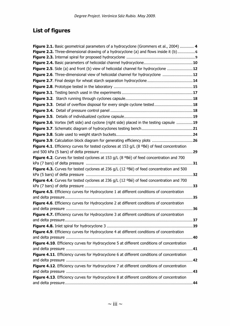
List of figures
Figure 2.1. Basic geometrical parameters of a hydrocyclone (Grommers et al., 2004) ............ 4 Figure 2.2. Three-dimensional drawing of a hydrocyclone (a) and flows inside it (b) ............... 6
Figure 2.3. Internal spiral for proposed hydrocyclone ........................................................... 9
Figure 2.4. Basic parameters of helicoidal channel hydrocyclone .......................................... 10
Figure 2.5. Side (a) and front (b) view of helicoidal channel for hydrocyclone ...................... 12
Figure 2.6. Three-dimensional view of helicoidal channel for hydrocyclone .......................... 12
Figure 2.7. Final design for wheat starch separation hydrocyclone ....................................... 14
Figure 2.8. Prototype tested in the laboratory .................................................................... 15
Figure 3.1. Testing bench used in the experiments ............................................................. 17
Figure 3.2. Starch running through cyclones capsule.......................................................... 18
Figure 3.3. Detail of overflow disposal for every single cyclone tested ................................. 18
Figure 3.4. Detail of pressure control panel ....................................................................... 18
Figure 3.5. Details of individualized cyclone capsule ........................................................... 19
Figure 3.6. Vortex (left side) and cyclone (right side) placed in the testing capsule .............. 19
Figure 3.7. Schematic diagram of hydrocyclones testing bench ............................................ 21
Figure 3.8. Scale used to weight starch buckets.................................................................. 24
Figure 3.9. Calculation block diagram for generating efficiency plots ................................... 26
Figure 4.1. Efficiency curves for tested cyclones at 153 g/L (8 ºBé) of feed concentration
and 500 kPa (5 bars) of delta pressure ................................................................................ 29
Figure 4.2. Curves for tested cyclones at 153 g/L (8 ºBé) of feed concentration and 700
kPa (7 bars) of delta pressure ............................................................................................ 31
Figure 4.3. Curves for tested cyclones at 236 g/L (12 ºBé) of feed concentration and 500
kPa (5 bars) of delta pressure ............................................................................................ 32
Figure 4.4. Curves for tested cyclones at 236 g/L (12 ºBé) of feed concentration and 700
kPa (7 bars) of delta pressure ............................................................................................. 33
Figure 4.5. Efficiency curves for Hydrocyclone 1 at different conditions of concentration
and delta pressure .............................................................................................................. 35
Figure 4.6. Efficiency curves for Hydrocyclone 2 at different conditions of concentration
and delta pressure ............................................................................................................. 36
Figure 4.7. Efficiency curves for Hydrocyclone 3 at different conditions of concentration
and delta pressure .............................................................................................................. 37
Figure 4.8. Inlet spiral for hydrocyclone 3 .......................................................................... 39
Figure 4.9. Efficiency curves for Hydrocyclone 4 at different conditions of concentration
and delta pressure ............................................................................................................. 40
Figure 4.10. Efficiency curves for Hydrocyclone 5 at different conditions of concentration
and delta pressure ............................................................................................................. 41
Figure 4.11. Efficiency curves for Hydrocyclone 6 at different conditions of concentration
and delta pressure ............................................................................................................. 42
Figure 4.12. Efficiency curves for Hydrocyclone 7 at different conditions of concentration
and delta pressure ............................................................................................................. 43
Figure 4.13. Efficiency curves for Hydrocyclone 8 at different conditions of concentration
and delta pressure .............................................................................................................. 44
Degree Project. Verónica Sáiz Rubio. May 2009.
~ iv ~
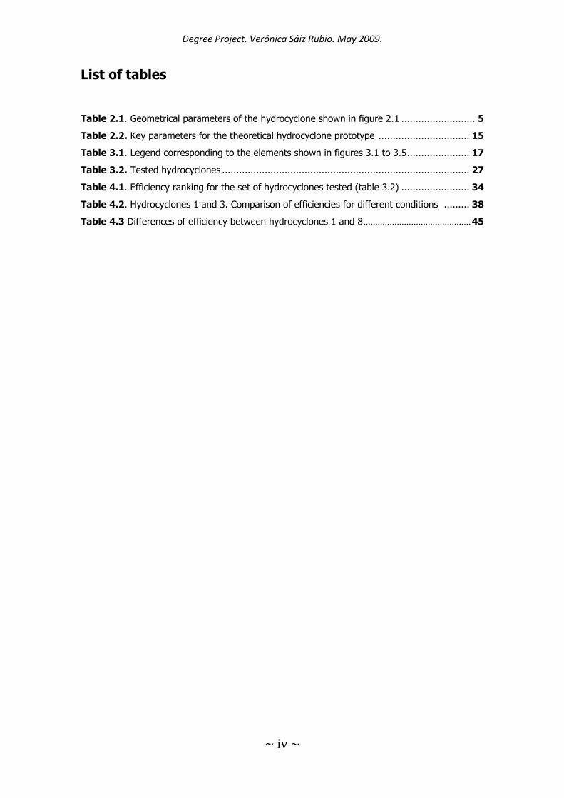
List of tables
Table 2.1. Geometrical parameters of the hydrocyclone shown in figure 2.1 .......................... 5
Table 2.2. Key parameters for the theoretical hydrocyclone prototype ................................ 15
Table 3.1. Legend corresponding to the elements shown in figures 3.1 to 3.5...................... 17
Table 3.2. Tested hydrocyclones ....................................................................................... 27
Table 4.1. Efficiency ranking for the set of hydrocyclones tested (table 3.2) ........................ 34
Table 4.2. Hydrocyclones 1 and 3. Comparison of efficiencies for different conditions ......... 38
Table 4.3 Differences of efficiency between hydrocyclones 1 and 8 ............................................. 45
Degree Project. Verónica Sáiz Rubio. May 2009.
~ 1 ~
Chapter 1
Introduction
An efficient separation of starch and protein in primary agricultural
products is vital for the food industry. Many basic grains such as tapioca
(Saengchan et al., 2009) or pin milled chickpea grain (Emami et al., 2005)
require a good separation of starch and protein for its further use. There exist
various physical methods for starch separation, and although Svarovsky (1984)
has suggested the use of hydrocyclones for starch separation for more than
twenty years, researchers are still investigating the benefits of cyclone
technology for physical separation. One such recent study is brought by Emami
et al. (2006), who compared the combination of hydrocyclone and centrifuge on
one hand, with the coupling of a centrifuge and a sieve on the other, for
separating starch and protein from chickpea flour. In this case, the process
involving the hydrocyclone was more efficient extracting the starch, but it also
included the aid of a centrifuge to achieve an acceptable separation rate.
Saengchan et al. (2009), on the contrary, used only a hydrocyclone system
instead of a centrifugal separator for tapioca starch separation; the optimum
selection of process parameters enhanced separation efficacy. In spite of its
economic importance, not only starch is the only application for hydrocyclone
separators; Habibian et al. (2008), for example, employed the same technique
for removing yeasts from alcohol fermentation broths. They concluded that
viscosity was a crucial factor affecting separation efficiency, and because this
technology could be applied to large molecules, starch appeared as a favorite
candidate for hydrocyclone separation. This research proved that a multi-
hydrocyclone system with low feed concentration is more efficient than one
single hydrocyclone dealing with higher feed concentrations, although lab
testing can be carried out with a single hydrocyclone (Emami et al., 2005).
The adequate geometry of a hydrocyclone, that is, its design, together
with the proper choice of working parameters is the safest preparation for an
efficient separation (Emami et al., 2006; Chu et al., 2000). According to
Degree Project. Verónica Sáiz Rubio. May 2009.
~ 2 ~
Grommers et al. (2004), small geometrical changes on the hydrocyclones have
strong influences on the outcomes. The set of process parameters can be
selected by pairs (Emami et al., 2005), or conversely by a threefold relationship
(Chu et al., 2002b). It is important to design the hydrocyclone according to the
target pursued (Chu et al., 2002a). The goal set by Chu et al. (2000) in their
design was getting the highest savings on energy consumption. To do so,
multiple parameter combinations were tested and graded based upon their
influence on power conservation. They found that the most influenceable
factors, sorted by relevance, were: central inserted parts, inlet pipes,
cyclindrical parts, vortex finders, cone parts and underflow pipes. Relevant
information about hydrocyclones design has been reported in specialized
journals; so, for example, pressures over 865 kPa may cause the appearance of
undesirable particles in the underflow (Emami et al., 2005), and when the
vortex finder length is about 10 % of the total length of the hydrocyclone high
efficiencies can be reached (Fernández Martínez et al., 2008). An interesting
phenomenon to consider is the formation of air cores (Gupta et al., 2008). The
air core is a strip of air extended vertically throughout the whole axis of the
cyclone provoked by the low pressures found in this place. Its effects can be
reduced by introducing a rod inside the hydrocyclone.
The overall objective of this research is the design, study, and analysis of
energy-saving hydrocyclones for wheat starch separation. This project took
place under the Erasmus Program of international students exchange between
Växjö University (Sweden) and the Polytechnic University of Valencia (Spain).
The collaborative framework between industry and academia at Växjö
University made possible the development of this investigation in the company
Larsson M. Verkstad AB, located in Bromölla (Sweden). Design and literature
search took place at Växjö University whereas the fabrication of the
hydrocyclones and their testing happened in two facilities operated by Larsson
in Bromölla and Linköping, both in Sweden. The duration of the project was
limited by academic constraints, which approximately allocated the six month of
the spring semester of 2009 to fulfill the goals set by both institutions. In
addition to meeting the academic requirements for achieving an engineering
Degree Project. Verónica Sáiz Rubio. May 2009.
~ 3 ~
degree, this investigation was intended to help Larsson improve their current
designs of hydrocyclones for starch separation, paying attention to energy-
saving properties and separation efficiency. This modus operandi resulted in a
very fruitful collaboration between the graduating student, her academic
advisors, and Larsson staff.
The specific goals proposed and accomplished in this research project
were the following:
1. The technical study and scientific review of hydrocyclones
geometry and starch separation techniques.
2. The proposal of a theoretical design of an energy-saving
hydrocyclone.
3. Laboratory testing of the designed hydrocyclone in comparison
with other models proposed by Larsson.
4. The enunciation of a set of recommendations for wheat starch
separation cyclones.
5. The publication of the results found in the project at the Annual
International Meeting held by the American Society of Agricultural
and Biological Engineers in Reno (Nevada, USA) in June 2009.
Degree Project. Verónica Sáiz Rubio. May 2009.
~ 4 ~
Chapter 2
Theoretical design of a hydrocyclone for starch separation
2.1. Geometry and mechanics of hydrocyclones
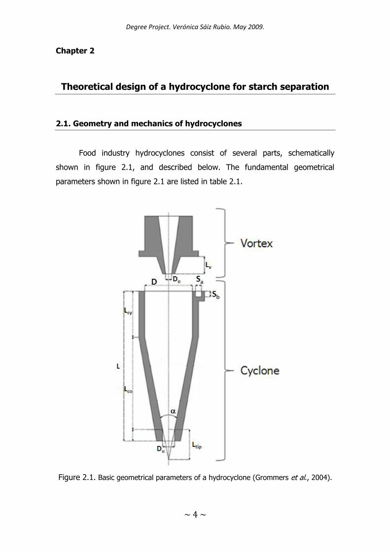
Food industry hydrocyclones consist of several parts, schematically
shown in figure 2.1, and described below. The fundamental geometrical
parameters shown in figure 2.1 are listed in table 2.1.
Figure 2.1. Basic geometrical parameters of a hydrocyclone (Grommers et al., 2004).
Degree Project. Verónica Sáiz Rubio. May 2009.
~ 5 ~
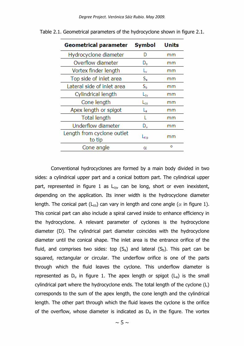
Table 2.1. Geometrical parameters of the hydrocyclone shown in figure 2.1.
Conventional hydrocyclones are formed by a main body divided in two
sides: a cylindrical upper part and a conical bottom part. The cylindrical upper
part, represented in figure 1 as Lcy, can be long, short or even inexistent,
depending on the application. Its inner width is the hydrocyclone diameter
length. The conical part (Lco) can vary in length and cone angle ( in figure 1).
This conical part can also include a spiral carved inside to enhance efficiency in
the hydrocyclone. A relevant parameter of cyclones is the hydrocyclone
diameter (D). The cylindrical part diameter coincides with the hydrocyclone
diameter until the conical shape. The inlet area is the entrance orifice of the
fluid, and comprises two sides: top (Sa) and lateral (Sb). This part can be
squared, rectangular or circular. The underflow orifice is one of the parts
through which the fluid leaves the cyclone. This underflow diameter is
represented as Du in figure 1. The apex length or spigot (La) is the small
cylindrical part where the hydrocyclone ends. The total length of the cyclone (L)
corresponds to the sum of the apex length, the cone length and the cylindrical
length. The other part through which the fluid leaves the cyclone is the orifice
of the overflow, whose diameter is indicated as Do in the figure. The vortex
Degree Project. Verónica Sáiz Rubio. May 2009.
~ 6 ~
finder length (Lv) is the part of the vortex assembled inside the cylindrical part
of the cyclone. The total length from cyclone outlet to tip (Ltip) indicates the
length from the end of the cyclone to the vertex where the cone part ends.
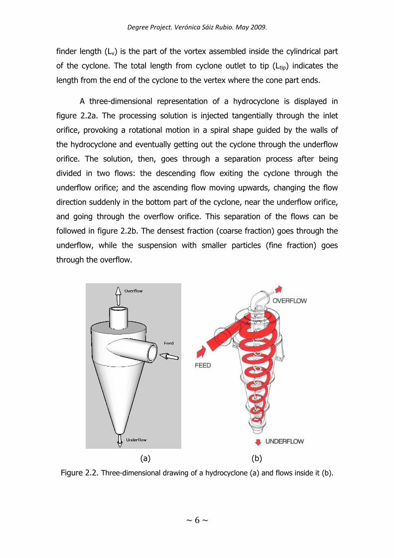
A three-dimensional representation of a hydrocyclone is displayed in
figure 2.2a. The processing solution is injected tangentially through the inlet
orifice, provoking a rotational motion in a spiral shape guided by the walls of
the hydrocyclone and eventually getting out the cyclone through the underflow
orifice. The solution, then, goes through a separation process after being
divided in two flows: the descending flow exiting the cyclone through the
underflow orifice; and the ascending flow moving upwards, changing the flow
direction suddenly in the bottom part of the cyclone, near the underflow orifice,
and going through the overflow orifice. This separation of the flows can be
followed in figure 2.2b. The densest fraction (coarse fraction) goes through the
underflow, while the suspension with smaller particles (fine fraction) goes
through the overflow.
(a) (b)
Figure 2.2. Three-dimensional drawing of a hydrocyclone (a) and flows inside it (b).
Degree Project. Verónica Sáiz Rubio. May 2009.
~ 7 ~
The actuating forces for a solid-liquid separation inside the hydrocyclone
are of two types: centrifugal and drag forces. Gravitational forces can be
neglected for small hydrocyclones, as those separating particles not bigger than
40 μm, like the wheat starch particles considered in this project. According to
Eliasson (2004), wheat starch particles are approximately 22 μm. When
centrifugal forces exceed drag forces, particles move outwards; in the opposite
case, particles will generally move inwards (Saengchan et al., 2009). The
separation principle of a hydrocyclone is based on inertial forces, because
circular trajectories induce radial accelerations. Flow density also influences the
separation success: if the solid fraction has a density higher than the fluid
density, the particles move around the wall and eventually leave the cyclone
through the underflow, but if the density of particles is lower than the fluid
density, the flow leaves the cyclone through the overflow exit (Fernández
Martínez et al., 2007).
2.2. Geometry of proposed hydrocyclone
The first design parameter to be determined is the hydrocyclone
diameter Dh. Many choices have been suggested by specialized manufacturers.
Larsson (Brömolla, Sweden), for example, features either 8 mm or 10 mm
hydrocyclones. Wheat starch particles have an average size of 22 μm (Eliasson,
2004) and the potato starch particle average size is 40 μm. Due to that fact, a
diameter of 8 mm should be suitable, as the common diameter for potato
starch is 10 mm, but, tapioca starch particle is smaller than that of wheat starch
and uses diameters of 10 mm, as well. Then, it was thought that would be
adequate to assume a diameter of 10 mm for wheat starch adding the
advantage to have higher capacity with that election. So, a diameter of 10 mm
has been selected.
The second element of the hydrocyclone to be designed is the inlet area.
This orifice can be squared, rectangular or circular in shape. The most efficient
models reported in the market, mainly applied to potato or tapioca starch
Degree Project. Verónica Sáiz Rubio. May 2009.
~ 8 ~
separation, include a rectangular or squared inlet section, and therefore this
was the shape chosen for the proposed design. However, a smaller size was
preferred in order to increase flow pressure and in turns enhance efficiency.
The final cyclone includes a square inlet section with a 2.1 mm side. The inlet
area is located in the upper edge of the hydrocyclone. From this edge, a spiral
carved inside the body of the cyclone can smooth the flow of starch and, in
consequence, raise the cyclone efficiency. The basic equation for the proposed
spiral is given in equation 1, where parameters and are determined from
the contour conditions shown in equation 2.
cosR [Eq. 1]
min
max
4RRIf
RRIf
[Eq. 2]
Applying the conditions of equation 2 to equation 1:
maxR [Eq. 3]
2
2minR [Eq. 4]
Withdrawing equation 4 from equation 3, we can find and can be obtained
directly from equation 3 once is known. The final formula is given in equation
6:
22
2 maxmin RR [Eq. 5]
,4
cos22
)(2
)22(
)(2 maxminmaxminmax
RRRRRR
[Eq. 6]
The conditions for the proposed hydrocyclone will be Rmax = 5.5 mm and Rmin =
5 mm. and the equation for this specific case is as follows:
,422
cos
)22(
15.5R [Eq. 7]
Degree Project. Verónica Sáiz Rubio. May 2009.
~ 9 ~
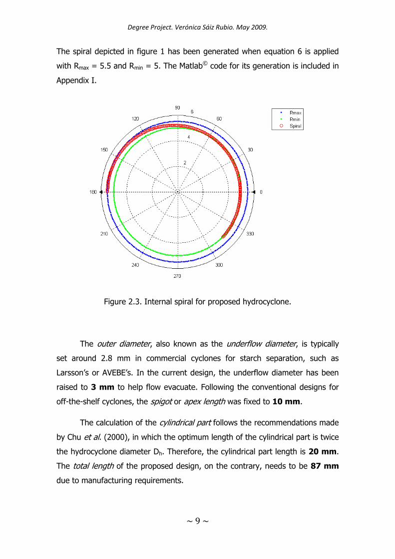
The spiral depicted in figure 1 has been generated when equation 6 is applied
with Rmax = 5.5 and Rmin = 5. The Matlab© code for its generation is included in
Appendix I.
Figure 2.3. Internal spiral for proposed hydrocyclone.
The outer diameter, also known as the underflow diameter, is typically
set around 2.8 mm in commercial cyclones for starch separation, such as
Larsson’s or AVEBE’s. In the current design, the underflow diameter has been
raised to 3 mm to help flow evacuate. Following the conventional designs for
off-the-shelf cyclones, the spigot or apex length was fixed to 10 mm.
The calculation of the cylindrical part follows the recommendations made
by Chu et al. (2000), in which the optimum length of the cylindrical part is twice
the hydrocyclone diameter Dh. Therefore, the cylindrical part length is 20 mm.
The total length of the proposed design, on the contrary, needs to be 87 mm
due to manufacturing requirements.

Degree Project. Verónica Sáiz Rubio. May 2009.
~ 10 ~
The hydrocyclone cone length is a geometrical parameter determined by
withdrawing the cylindrical and spigot lengths from the total length of the
cyclone. Applying the specifications found above, the cone length for the
proposed design is 57 mm. Along the length of the cone part, it is possible to
engrave a spiral creating a helicoidal channel. This channel can improve the
cyclone’s efficiency. The mathematical determination of the helicoidal channel
for the proposed cyclone is provided in full detail in the following paragraphs.
The basic parameters needed to formulate the helicoidal channel are:
Rmax: maximum radius of the cone
Rmin: minimum radius of the cone
Le: Helix pitch
L: Total length of conical section of cyclone
[x,y,z]: Cartesian coordinates as indicated in figure 2.4.
Figure 2.4. Basic parameters of helicoidal channel
The radius of the helix is variable and depends on the cone shape. It can be
easily calculated with equations 8 and 9.
L
zLRR minmax [Eq. 8]
],0[minmaxminmin LzL
zLRRRRR [Eq. 9]
Degree Project. Verónica Sáiz Rubio. May 2009.
~ 11 ~
It can be checked with equation 9 that If Z = 0, R = Rmax; and similarly, if Z =
L, R = Rmin.
Before deducing the equation of the helix, or spiral, the number of loops (n)
needs to be obtained through the expression given in equation 10, where the
function int forces n to be integer.
eL
Ln int [Eq. 10]
The parametric equations of the three-dimensional helix are finally stated in
equation 11:
mminzyxnt
tL
z
tL
zLRRRy
tL
zLRRRx
e
,,2,0
2
)sin(
)cos(
minmaxmin
minmaxmin
[Eq. 11]
The expression shown in equation 11 provides the Cartesian coordinates
of a generic point [x, y, z] belonging to the spiral, but the proposed
hydrocyclone possesses very specific dimensions as described in the previous
paragraphs. In particular, the following parameters have been determined for
the calculated design: Rmax = 5 mm, Rmin = 1.5 mm, Le = 5 mm, and L = 57
mm [zmax]. After applying these figures to equation 11 the concrete helix to be
traced inside the cone part is defined by equation 12 below.
22,0
2
5
)sin(57
5.3285
)cos(57
5.3285
t
tz
tz
y
tz
x
[Eq. 12]
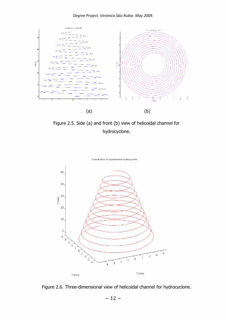
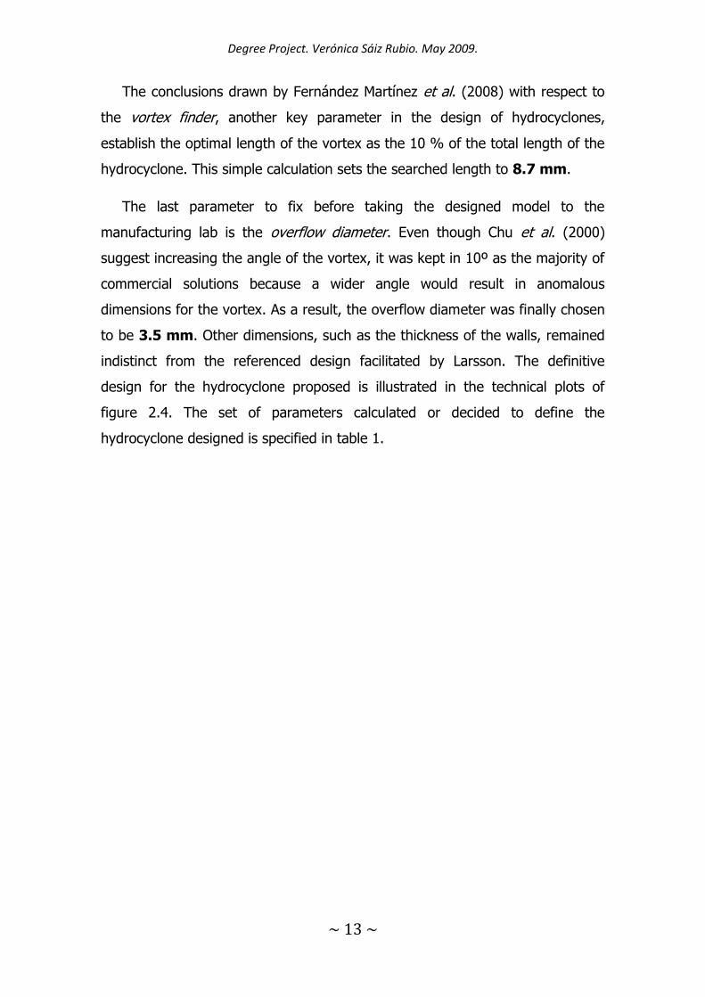
The helix determined by the expression of equation 12 was plotted with
Matlab© (code provided in Appendix II). A side view of the spiral is depicted in
figure 2.3 (a), and its front view is given in figure 2.3 (b). The three-
dimensional view of the helix is plotted in figure 2.4.
Degree Project. Verónica Sáiz Rubio. May 2009.
~ 12 ~
(a) (b)
Figure 2.5. Side (a) and front (b) view of helicoidal channel for
hydrocyclone.
Figure 2.6. Three-dimensional view of helicoidal channel for hydrocyclone.
Degree Project. Verónica Sáiz Rubio. May 2009.
~ 13 ~
The conclusions drawn by Fernández Martínez et al. (2008) with respect to
the vortex finder, another key parameter in the design of hydrocyclones,
establish the optimal length of the vortex as the 10 % of the total length of the
hydrocyclone. This simple calculation sets the searched length to 8.7 mm.
The last parameter to fix before taking the designed model to the
manufacturing lab is the overflow diameter. Even though Chu et al. (2000)
suggest increasing the angle of the vortex, it was kept in 10º as the majority of
commercial solutions because a wider angle would result in anomalous
dimensions for the vortex. As a result, the overflow diameter was finally chosen
to be 3.5 mm. Other dimensions, such as the thickness of the walls, remained
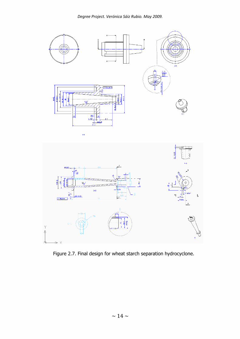
indistinct from the referenced design facilitated by Larsson. The definitive
design for the hydrocyclone proposed is illustrated in the technical plots of
figure 2.4. The set of parameters calculated or decided to define the
hydrocyclone designed is specified in table 1.
Degree Project. Verónica Sáiz Rubio. May 2009.
~ 14 ~
Figure 2.7. Final design for wheat starch separation hydrocyclone.

Degree Project. Verónica Sáiz Rubio. May 2009.
~ 15 ~
Table 2.2. Key parameters for the theoretical hydrocyclone prototype.
PARAMETER VALUE
Hydrocyclone diameter 10 mm
Inlet area 2.1 x 2.1 mm2
Underflow diameter 3 mm
Apex length 10 mm
Cylindrical length 20 mm
Total length 87 mm
Cone part 57 mm
Vortex finder length 8.7 mm
Overflow diameter 3.5 mm
Figure 2.8. Prototype tested in the laboratory.
Degree Project. Verónica Sáiz Rubio. May 2009.
~ 16 ~
Chapter 3
Materials and methods
The objective of the experiments proposed was to know the efficiency of
each hydrocyclone especially designed to reduce energy costs; therefore, the
first task to do was the design of the experiments and the selection of all
parameters needed. An ExcelTM file was prepared to process the data as the
trials were being performed. The main parameters considered in the tests were:
underflow pressure (kPa), feed concentration (g/L), delta pressure (kPa), feed
volume (L), overflow volume (L), underflow volume (L), feed concentration
(g/L), overflow concentration (g/L), underflow concentration (g/L), weight
overflow (kg), weight underflow (kg), time overflow (s), time underflow (s),
temperature (ºC), feed flow (cm3/s), underflow flow (cm3/s), overflow flow
(cm3/s), flow ratio (dimensionless) and efficiency (dimensionless). Once the
main variables were chosen, the set of experimental hydrocyclones were
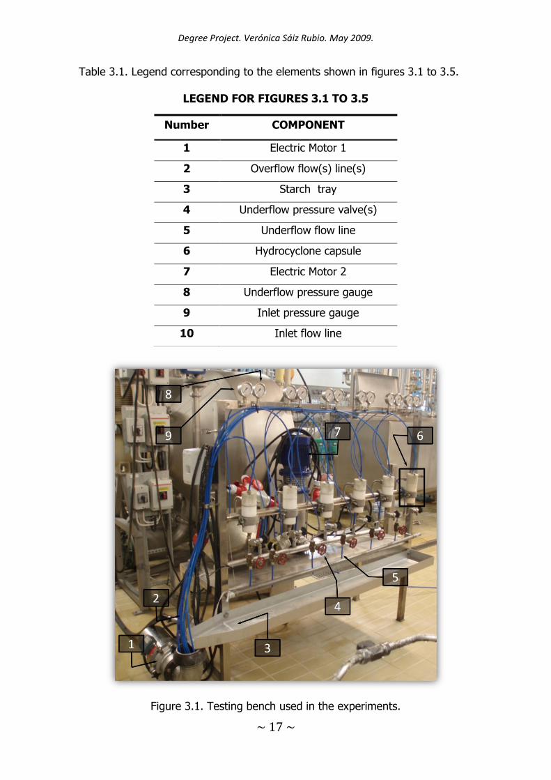
introduced in an especially-built testing machine developed by Larsson, and
represented in figure 3.1. The main components of the testing bench shown in
figures 3.1 to 3.5 are indicated by numbers whose correspondence is included
in table 3.1.
Degree Project. Verónica Sáiz Rubio. May 2009.
~ 17 ~
Table 3.1. Legend corresponding to the elements shown in figures 3.1 to 3.5.
Figure 3.1. Testing bench used in the experiments.
LEGEND FOR FIGURES 3.1 TO 3.5
Number COMPONENT
1 Electric Motor 1
2 Overflow flow(s) line(s)
3 Starch tray
4 Underflow pressure valve(s)
5 Underflow flow line
6 Hydrocyclone capsule
7 Electric Motor 2
8 Underflow pressure gauge
9 Inlet pressure gauge
10 Inlet flow line
Degree Project. Verónica Sáiz Rubio. May 2009.
~ 18 ~
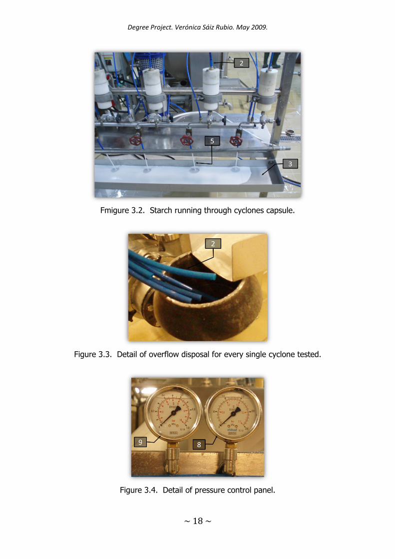
Fmigure 3.2. Starch running through cyclones capsule.
Figure 3.3. Detail of overflow disposal for every single cyclone tested.
Figure 3.4. Detail of pressure control panel.
Degree Project. Verónica Sáiz Rubio. May 2009.
~ 19 ~
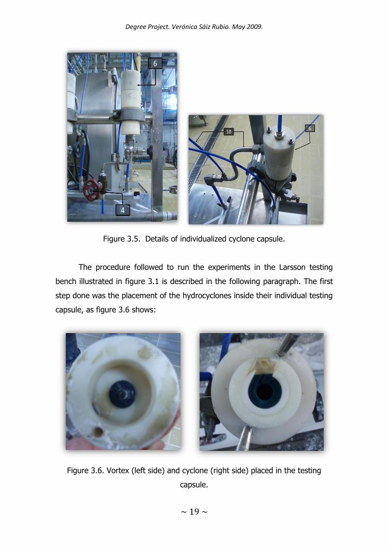
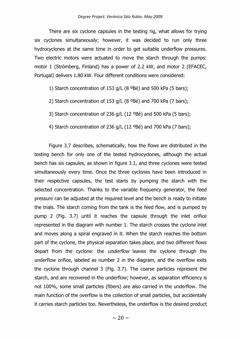
Figure 3.5. Details of individualized cyclone capsule.
The procedure followed to run the experiments in the Larsson testing
bench illustrated in figure 3.1 is described in the following paragraph. The first
step done was the placement of the hydrocyclones inside their individual testing
capsule, as figure 3.6 shows:
Figure 3.6. Vortex (left side) and cyclone (right side) placed in the testing
capsule.
Degree Project. Verónica Sáiz Rubio. May 2009.
~ 20 ~
There are six cyclone capsules in the testing rig, what allows for trying
six cyclones simultaneously; however, it was decided to run only three
hydrocyclones at the same time in order to get suitable underflow pressures.
Two electric motors were actuated to move the starch through the pumps:
motor 1 (Strömberg, Finland) has a power of 2.2 kW, and motor 2 (EFACEC,
Portugal) delivers 1.80 kW. Four different conditions were considered:
1) Starch concentration of 153 g/L (8 ºBé) and 500 kPa (5 bars);
2) Starch concentration of 153 g/L (8 ºBé) and 700 kPa (7 bars);
3) Starch concentration of 236 g/L (12 ºBé) and 500 kPa (5 bars);
4) Starch concentration of 236 g/L (12 ºBé) and 700 kPa (7 bars);
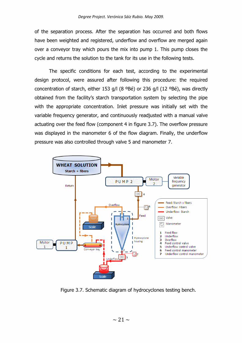
Figure 3.7 describes, schematically, how the flows are distributed in the
testing bench for only one of the tested hydrocyclones, although the actual
bench has six capsules, as shown in figure 3.1, and three cyclones were tested
simultaneously every time. Once the three cyclones have been introduced in
their respective capsules, the test starts by pumping the starch with the
selected concentration. Thanks to the variable frequency generator, the feed
pressure can be adjusted at the required level and the bench is ready to initiate
the trials. The starch coming from the tank is the feed flow, and is pumped by
pump 2 (Fig. 3.7) until it reaches the capsule through the inlet orifice
represented in the diagram with number 1. The starch crosses the cyclone inlet
and moves along a spiral engraved in it. When the starch reaches the bottom
part of the cyclone, the physical separation takes place, and two different flows
depart from the cyclone: the underflow leaves the cyclone through the
underflow orifice, labeled as number 2 in the diagram, and the overflow exits
the cyclone through channel 3 (Fig. 3.7). The coarse particles represent the
starch, and are recovered in the underflow; however, as separation efficiency is
not 100%, some small particles (fibers) are also carried in the underflow. The
main function of the overflow is the collection of small particles, but accidentally
it carries starch particles too. Nevertheless, the underflow is the desired product
Degree Project. Verónica Sáiz Rubio. May 2009.
~ 21 ~
of the separation process. After the separation has occurred and both flows
have been weighted and registered, underflow and overflow are merged again
over a conveyor tray which pours the mix into pump 1. This pump closes the
cycle and returns the solution to the tank for its use in the following tests.
The specific conditions for each test, according to the experimental
design protocol, were assured after following this procedure: the required
concentration of starch, either 153 g/l (8 ºBé) or 236 g/l (12 ºBé), was directly
obtained from the facility’s starch transportation system by selecting the pipe
with the appropriate concentration. Inlet pressure was initially set with the
variable frequency generator, and continuously readjusted with a manual valve
actuating over the feed flow (component 4 in figure 3.7). The overflow pressure
was displayed in the manometer 6 of the flow diagram. Finally, the underflow
pressure was also controlled through valve 5 and manometer 7.
Figure 3.7. Schematic diagram of hydrocyclones testing bench.
Degree Project. Verónica Sáiz Rubio. May 2009.
~ 22 ~
These experiments were carried out in a facility operated by Larsson at
Reppe (Lidköping, Sweden). Two specific starch concentrations were
determined for the set of experiments: 153 g/L (8 ºBé) and 236 g/L (12 ºBé).
The real value for the concentration of starch can be estimated in two different
ways: using an aerometer or using a centrifuge machine. In these experiments,
the latter method was employed because it is considered the most reliable. To
get the concentration measurements, several test tubes of 10 ml volume were
filled with the dissolution of water and starch especially prepared by the facility
technician. The test tubes were introduced into the centrifuge machine and run
for 5 minutes at 3750 rpm. After centrifuging them, three phases were
separated: water, fibers and starch. The amount of starch found in the test
tubes, expressed in millimetres, was registered, as well as the amount of starch
plus fibers plus water, also in millimetres. The conversion from amount of
millimetres into Baumé degrees is shown in equation 3.1.
[Eq. 3.1]
The feed calculated through equation 3.1 was used to know the
approximate value of the starch concentrations, but it was not employed in
successive calculations. It was considered as a rough estimate of the
concentrations. Before trying the cyclones, it was necessary to make sure that
the required concentration of starch was available, together with the right inlet
pressure. In this particular case, the value of delta pressure was almost the
same as the inlet pressure, which was adjusted to 500 kPa (5 bars) or 700 kPa
(7 bars) depending on the trial. The reason why inlet pressure and delta
pressure can be considered the same is a consequence of the definition of delta
pressure as the difference between the inlet (or feed) pressure and the
overflow pressure. The overflow pressure was, in these tests, thirty centimetres
of water column measured at the hydrocyclone capsule, which means that the
overflow pressure is about 30 kPa (0.3 bars). These 30 kPa (0.3 bars) can be
approximated to zero, and if the overflow pressure is considered to be zero,
then the delta pressure is just the inlet pressure. The adjustment for the inlet
Degree Project. Verónica Sáiz Rubio. May 2009.
~ 23 ~
pressure was made with the help of a variable frequency generator and
displayed in the inlet manometer (figure 3.4, number 9). Once these initial
conditions were established, the underflow pressure for each hydrocyclone
tested was set up. The underflow pressure was chosen arbitrarily; it started
from low pressures and increased up to the point where it was still possible to
get enough flow of starch. Before the end of each trial, the curve obtained was
checked to assure that it had enough points to be represented. The underflow
pressure values give a reference of where the X-axis points will be located. The
underflow pressure was adjusted with a manual valve (fig. 3.5, number 4) and
shown in the underflow manometer (fig. 3.4, number 8). For each pressure
point tried and hydrocyclone tested, two samples of starch dissolution were
analyzed. Two test tubes were filled with the starch dissolution: one with starch
coming from the underflow flow, and the other with the starch dragged by the
overflow current. This procedure was executed for the three hydrocyclones
being tested at the same time. Concurrently, two test tubes filled with feed flow
were measured to check that the inlet concentration was exposed to the same
conditions every time. A 2 liter bucket was filled with underflow flow and
another bucket of the same volume was filled with overflow flow. The time
needed to fill up the buckets was registered in seconds. After taking several
samples, the test tubes were put into the centrifuge for 5 minutes at 3750 rpm,
separating the starch and leading to the calculation of millilitres of starch and
total millilitres, that is, an estimate of the overflow and underflow volumes. The
equations applied for the calculation of the overflow and underflow are
equations 3.2 and 3.3 respectively.
[Eq. 3.2]
[Eq. 3.3]
Degree Project. Verónica Sáiz Rubio. May 2009.
~ 24 ~
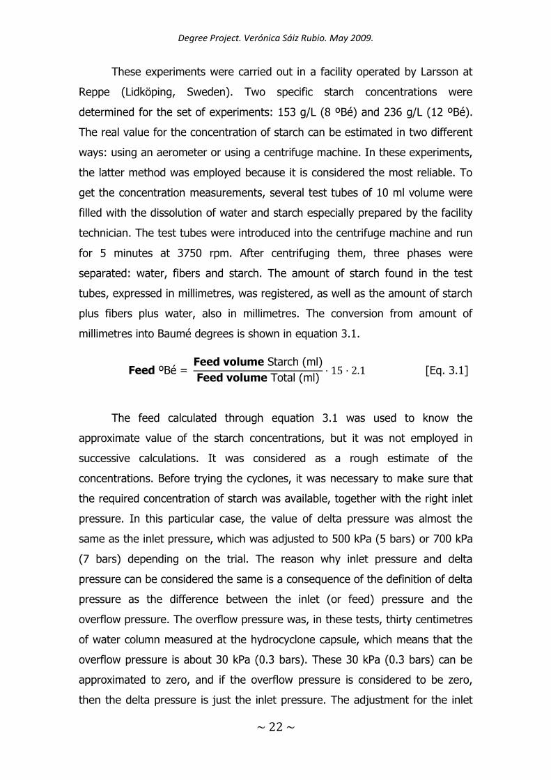
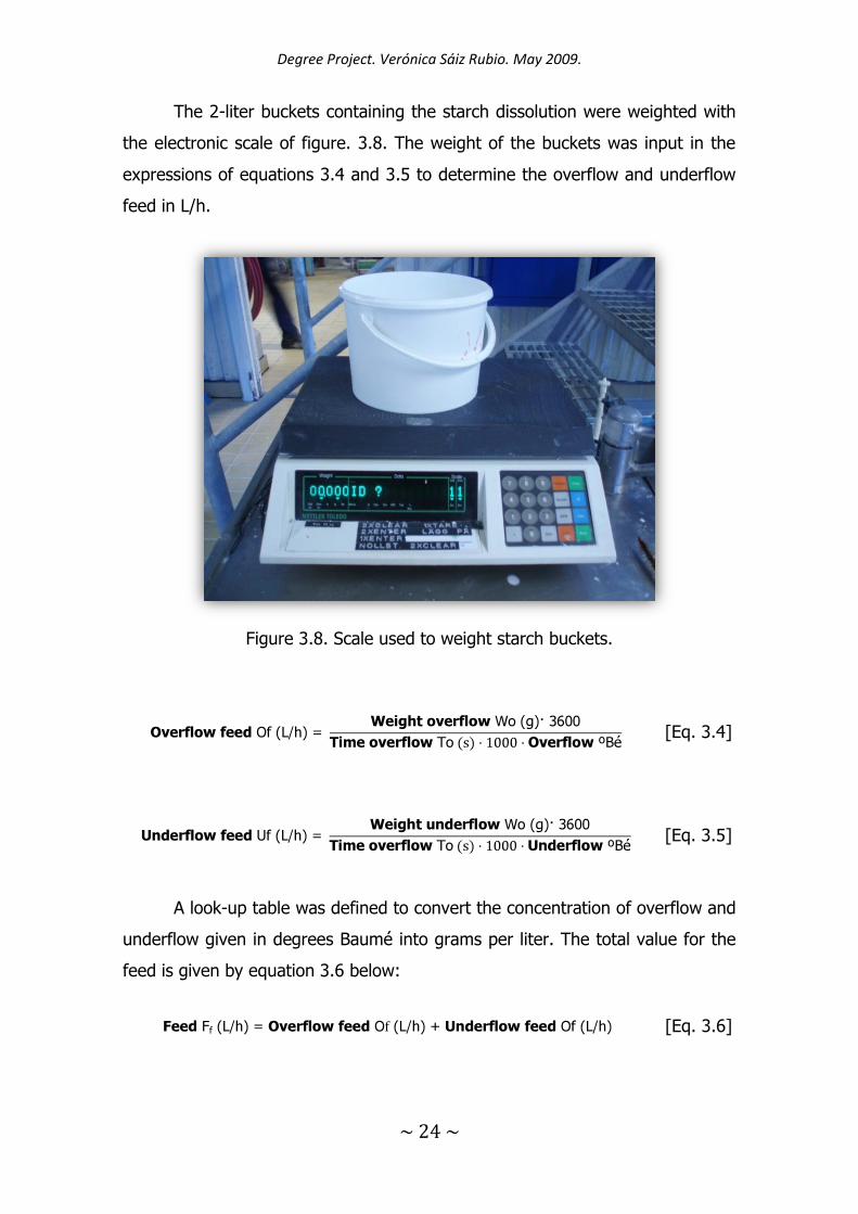
The 2-liter buckets containing the starch dissolution were weighted with
the electronic scale of figure. 3.8. The weight of the buckets was input in the
expressions of equations 3.4 and 3.5 to determine the overflow and underflow
feed in L/h.
Figure 3.8. Scale used to weight starch buckets.
[Eq. 3.4]
[Eq. 3.5]
A look-up table was defined to convert the concentration of overflow and
underflow given in degrees Baumé into grams per liter. The total value for the
feed is given by equation 3.6 below:
[Eq. 3.6]
Degree Project. Verónica Sáiz Rubio. May 2009.
~ 25 ~
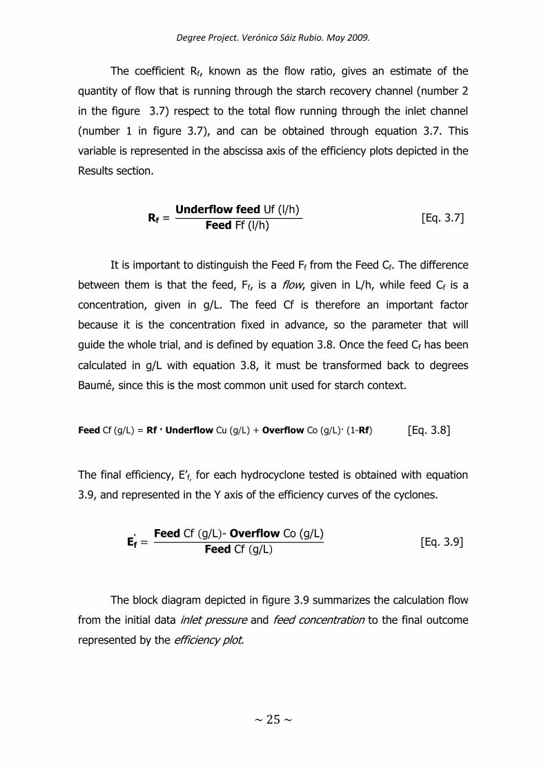
The coefficient Rf, known as the flow ratio, gives an estimate of the
quantity of flow that is running through the starch recovery channel (number 2
in the figure 3.7) respect to the total flow running through the inlet channel
(number 1 in figure 3.7), and can be obtained through equation 3.7. This
variable is represented in the abscissa axis of the efficiency plots depicted in the
Results section.
[Eq. 3.7]
It is important to distinguish the Feed Ff from the Feed Cf. The difference
between them is that the feed, Ff, is a flow, given in L/h, while feed Cf is a
concentration, given in g/L. The feed Cf is therefore an important factor
because it is the concentration fixed in advance, so the parameter that will
guide the whole trial, and is defined by equation 3.8. Once the feed Cf has been
calculated in g/L with equation 3.8, it must be transformed back to degrees
Baumé, since this is the most common unit used for starch context.
[Eq. 3.8]
The final efficiency, E’f, for each hydrocyclone tested is obtained with equation
3.9, and represented in the Y axis of the efficiency curves of the cyclones.
[Eq. 3.9]
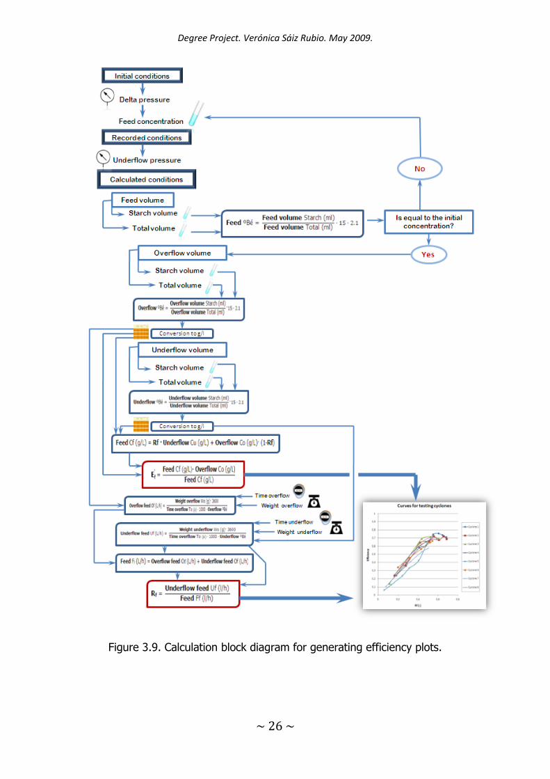
The block diagram depicted in figure 3.9 summarizes the calculation flow
from the initial data inlet pressure and feed concentration to the final outcome
represented by the efficiency plot.
Degree Project. Verónica Sáiz Rubio. May 2009.
~ 26 ~
Figure 3.9. Calculation block diagram for generating efficiency plots.
Degree Project. Verónica Sáiz Rubio. May 2009.
~ 27 ~
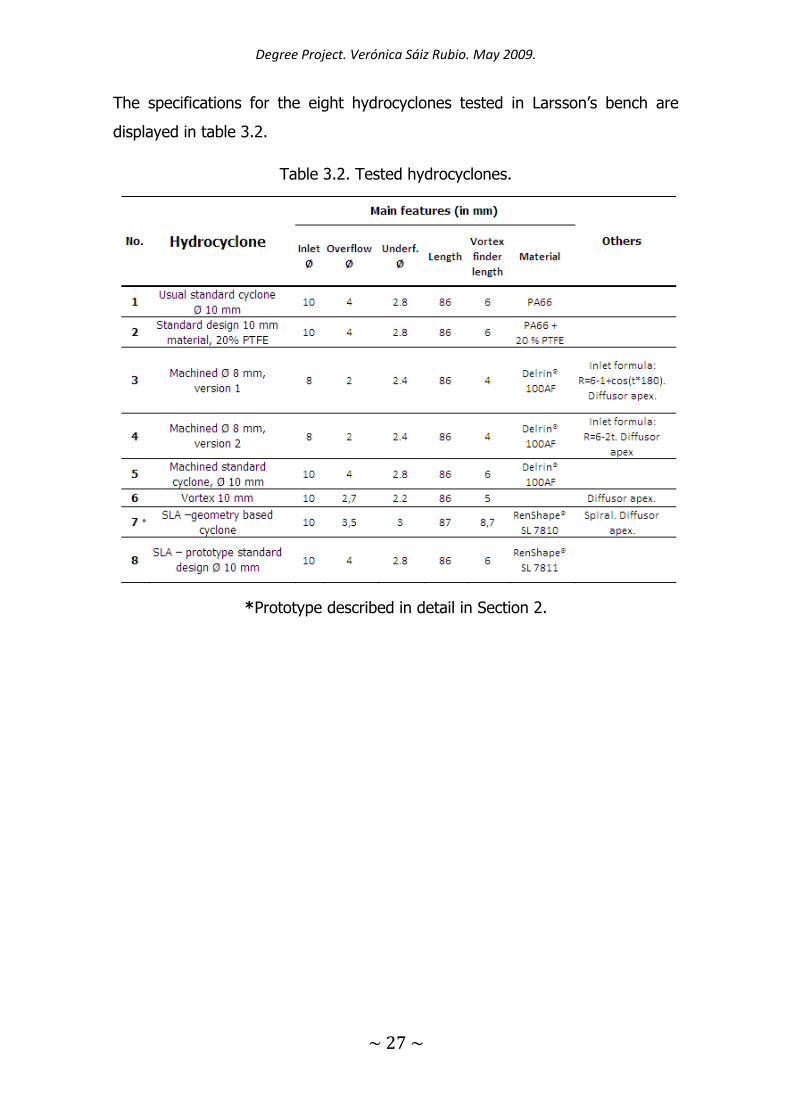
The specifications for the eight hydrocyclones tested in Larsson’s bench are
displayed in table 3.2.
Table 3.2. Tested hydrocyclones.
*Prototype described in detail in Section 2.
Degree Project. Verónica Sáiz Rubio. May 2009.
~ 28 ~
Chapter 4
Results and discussion
The overall objective of this research was to modify the current design of
hydrocyclones to improve efficiency, from the energy consumption point of
view, when separating starch from wheat. The initial idea consisted of limiting
pressure to 500 kPa (5 bars) while processing high concentrations of starch,
resulting in a low energy profile but high separation rate, reducing energy and
costs, which is the main goal of this study.
The efficiency curves of the hydrocyclones were built representing the
flow ratio (Rf) values in the X axis and the Efficiency (E’f) values in the Y axis.
Every graph depicts the efficiency curve of the eight cyclones tested for each
specific testing condition of concentration and pressure. Consequently, the
results of the experiments can be graphically represented in four different plots,
one for each different condition. The four combinations of pressure and
concentration were the following:
1) 153 g/L (8 ºBé) and 500 kPa (5 bars)
2) 153 g/L (8 ºBé) and 700 kPa (7 bars)
3) 236 g/L (12 ºBé) and 500 kPa (5 bars)
4) 236 g/L (12 ºBé) and 700 kPa (7 bars).
Every condition was applied to the set of eight experimental cyclones,
and therefore, every efficiency plot includes eight curves, one for each cyclone.
This procedure allows the fair comparison of the cyclones as testing conditions
were exactly the same. Additionally, the individual performance of each cyclone
for the four combinations of pressure and concentration tried is also plotted in
separated figures. These curves show the best working conditions for each
hydrocyclone proposed. The design goal for the cyclones is to find the best
geometry to increase the pressure inside the cyclone without increasing inlet
Degree Project. Verónica Sáiz Rubio. May 2009.
~ 29 ~
pressure, maintaining, or raising, the separation efficiency without incurring in
energy losses.
The technical specifications of the eight hydrocyclones tested are
provided in table 3.2.
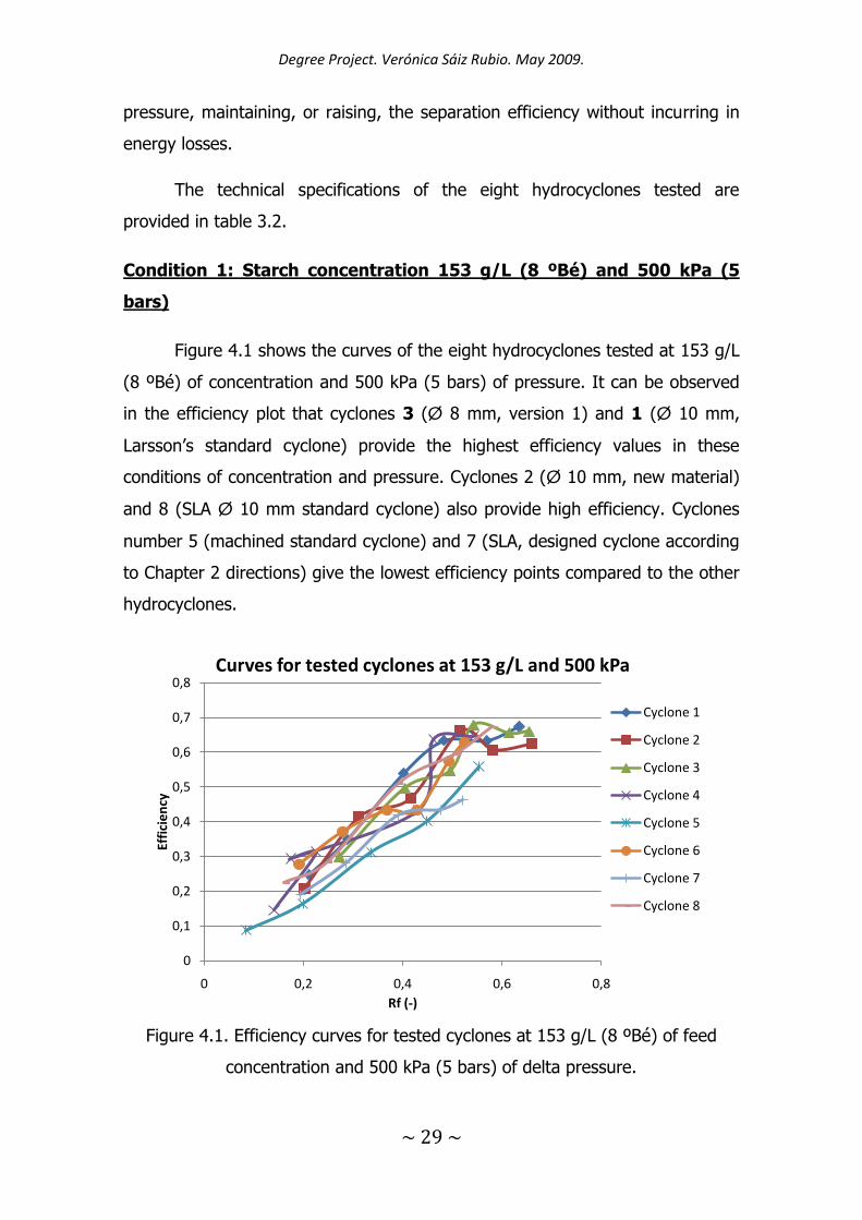
Condition 1: Starch concentration 153 g/L (8 ºBé) and 500 kPa (5
bars)
Figure 4.1 shows the curves of the eight hydrocyclones tested at 153 g/L
(8 ºBé) of concentration and 500 kPa (5 bars) of pressure. It can be observed
in the efficiency plot that cyclones 3 (Ø 8 mm, version 1) and 1 (Ø 10 mm,
Larsson’s standard cyclone) provide the highest efficiency values in these
conditions of concentration and pressure. Cyclones 2 (Ø 10 mm, new material)
and 8 (SLA Ø 10 mm standard cyclone) also provide high efficiency. Cyclones
number 5 (machined standard cyclone) and 7 (SLA, designed cyclone according
to Chapter 2 directions) give the lowest efficiency points compared to the other
hydrocyclones.
Figure 4.1. Efficiency curves for tested cyclones at 153 g/L (8 ºBé) of feed
concentration and 500 kPa (5 bars) of delta pressure.
0
0,1
0,2
0,3
0,4
0,5
0,6
0,7
0,8
0 0,2 0,4 0,6 0,8
Effi
cie
ncy
Rf (-)
Curves for tested cyclones at 153 g/L and 500 kPa
Cyclone 1
Cyclone 2
Cyclone 3
Cyclone 4
Cyclone 5
Cyclone 6
Cyclone 7
Cyclone 8
Degree Project. Verónica Sáiz Rubio. May 2009.
~ 30 ~
Condition 2: Starch concentration 153 g/L (8 ºBé) and pressure 700
kPa (7 bars)
For the next condition tried, the inlet pressure was increased up to 700
kPa (7 bars). The results of the hydrocyclones in these new conditions are
shown in figure 4.2. It can be observed that as the pressure increased so did
the efficiency. This fact was expected given the direct relationship between
pressure and efficiency (Svarovsky, 1984). Cyclones 1, 2, 3 and 8 were, again,
the most efficient. A concentration of 153 g/L (8 ºBé) with the pressure of 700
kPa (7 bars) made the overall efficiency increase. In consequence, the curves
were above the previous case. One reason for this outcome is the direct
relationship between pressure and efficiency, but another cause can be found
in the inverse relationship between efficiency and concentration (Svarovsky,
1984). At a “low” concentration of 153 g/L (8 ºBé; note that 153 g/L will be
considered a low concentration hereafter compared to 236 g/L (12 ºBé), which
will be considered a high concentration in this study), the efficiency is expected
to be higher than at high concentrations of starch. The average efficiency for
153 g/L (8 ºBé) and 700 kPa (7 bars) when the Rf is over 0.4 is around 70 %.
The relative comparison among cyclones also shows an advantage of 1, 2, 3
and 8 over 5 and 7. The highest value of efficiency reached in this testing
condition was obtained for hydrocyclone 1, with a top value of 76 %.

Degree Project. Verónica Sáiz Rubio. May 2009.
~ 31 ~
Figure 4.2. Curves for tested cyclones at 153 g/L (8 ºBé) of feed concentration
and 700 kPa (7 bars) of delta pressure.
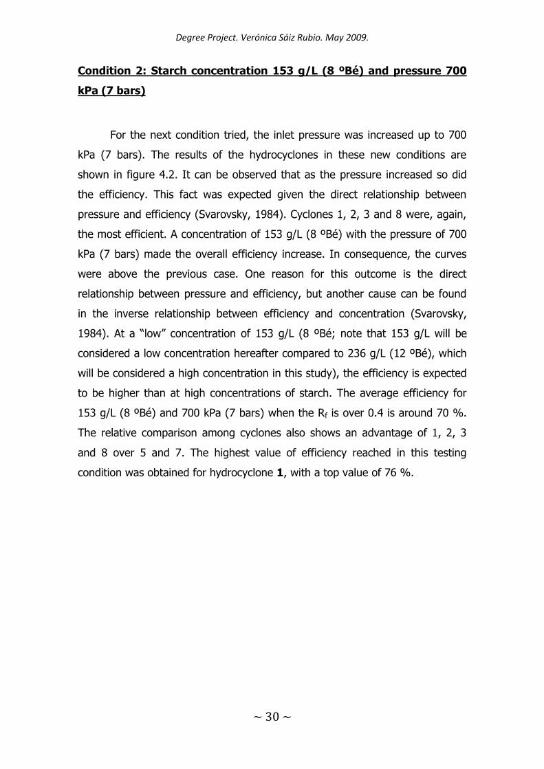
Condition 3: Starch concentration 236 g/L (12 ºBé) and pressure 500
kPa (5 bars)
In Condition 3, concentration was increased to 236 g/L (12 ºBé) and
delta pressure was set at 500 kPa (5 bars). According to the considerations
made in this study, pressure is labeled low in this case and concentration high.
A low pressure is preferable because it saves energy and reduces costs. High
concentration is also preferable because the separation process is faster.
Therefore, this study case initially presents more advantages than the rest, but
the hydrocyclones need to respond accordingly yielding higher efficiencies.
The first apparent difference of the efficiency plot of figure 4.3, in
comparison to figures 4.1 and 4.2, is the shape of the curves. All the curves for
Condition 3 do not reach an efficiency peak after which they decrease again;
the curve grows monotonically without reaching a local maxima. The peaks of
the curves were limited by the settings of the underflow pressure valve. In this
0
0,1
0,2
0,3
0,4
0,5
0,6
0,7
0,8
0 0,2 0,4 0,6 0,8
Effi
cie
ncy
Rf (-)
Curves for testing cyclones at 153 g/L and 700 kPa
Cyclone 1
Cyclone 2
Cyclone 3
Cyclone 4
Cyclone 5
Cyclone 6
Cyclone 7
Cyclone 8
Degree Project. Verónica Sáiz Rubio. May 2009.
~ 32 ~
particular test, the highest points of the curves were reached at the specific
points of Rf when the valve for controlling the underflow pressure was totally
open, so the lowest underflow pressures and the highest flows to the underflow
led to the maximum efficiency.
The hydrocyclone that reached the highest point of efficiency in these
conditions of concentration and pressure was number 3 (Ø 8 mm, version 1),
with a value of 66 %. The second highest efficiency was found with cyclone 4
(Ø 8 mm, version 2). These results prove that a smaller cyclone diameter has a
positive effect on the energy-saving features of starch cyclones. The anomalous
behavior of cyclone 5 was caused by a metal piece accidentally deposited in the
inlet. Since there was no possibility of repeating the experiments after removing
the metal part, no conclusions can be drawn for cyclone 5 under Condition 3.
Figure 4.3. Curves for tested cyclones at 236 g/L (12 ºBé) of feed concentration
and 500 kPa (5 bars) of delta pressure.
0
0,1
0,2
0,3
0,4
0,5
0,6
0,7
0 0,2 0,4 0,6 0,8
Effi
cie
ncy
Rf (-)
Efficiency curves for cyclones at 237 g/L and 500 kPa
Cyclone 1
Cyclone 2
Cyclone 3
Cyclone 4
Cyclone 5
Cyclone 6
Cyclone 7
Cyclone 8
Degree Project. Verónica Sáiz Rubio. May 2009.
~ 33 ~
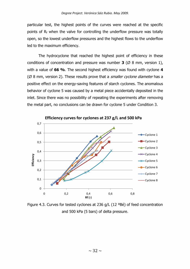
Condition 4: Starch concentration 236 g/L (12 ºBé) and pressure 700
kPa (7 bars)
The last testing conditions gave the efficiency plot of figure 4.4. When
the starch concentration is 236 g/L (12 °Bé) and the delta pressure is 700 kPa
(7 bars), cyclone 8 (SLA Ø 10 mm standard cyclone) reached the highest
efficiency. The second highest efficiency was found with cyclone 5. This
favorable result for cyclone 5 indicates its high potential for the previous
conditions had the unfortunate metal part not ended up inside the inlet. This
situation should be investigated in the future.
In general, low pressures produce more variability in the efficiency than
high pressures, this is, the curves for low pressure conditions present a wider
range of operation while high pressure curves are closer to each other, as
shown in figure 4.4.
Figure 4.4. Curves for tested cyclones at 236 g/L (12 ºBé) of feed concentration
and 700 kPa (7 bars) of delta pressure.
0
0,1
0,2
0,3
0,4
0,5
0,6
0,7
0 0,2 0,4 0,6 0,8
Effi
cie
ncy
Rf (-)
Curves for tested cyclones at 236 g/L and 700 kPa
Cyclone 1
Cyclone 2
Cyclone 3
Cyclone 4
Cyclone 5
Cyclone 6
Cyclone 7
Cyclone 8

Degree Project. Verónica Sáiz Rubio. May 2009.
~ 34 ~
The results of the experiments under the four conditions of concentration
and pressure tested are summarized in table 4.1. One of the most important
findings this table is showing is that hydrocyclone number 3 is the one that
gives the highest efficiency even in low pressure conditions (500 kPa). As a
result, this cyclone was the most appropriate for low pressures. Conversely,
results were not so homogeneous when inlet pressure was set to 700 kPa.
Given that one of the ways to reduce energy consumption is by keeping a low
inlet pressure, and cyclone 3 performs well for both concentrations tried, the
results of the experiments suggest that cyclone 3 operating at 500 kPa and 236
g/L is the most reasonable option of the set tried. Other cyclones with
encouraging results which can be considered potential solutions are
hydrocyclones 4, 1 and 8, in decreasing order of preference according to the
desirable conditions of low pressure and high concentration. As hydrocyclone 2
also behaves acceptably for low pressures, it should be taken into account in
the future as well.
Table 4.1. Efficiency ranking for the set of hydrocyclones tested (table 3.2).
Concentration (g/L) 153 153 237 237
Delta pressure (kPa) 500 700 500 700
1st position 3 1 3 8
2nd position 1 2 4 4
3rd position 8 3 1 5
4th position 2 8 8 2 & 3
Individual performance of the hydrocyclones for all the conditions
tested
Once a hydrocyclone has been selected, it is very interesting to see how
it behaves when working conditions vary. The following discussion takes this
idea into account and bases its conclusions on the graphical representation of
the efficiency for each cyclone when conditions change according to the
directions given by table 4.1.
Degree Project. Verónica Sáiz Rubio. May 2009.
~ 35 ~
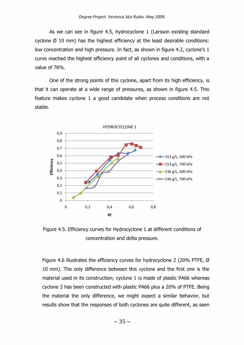
As we can see in figure 4.5, hydrocyclone 1 (Larsson existing standard
cyclone Ø 10 mm) has the highest efficiency at the least desirable conditions:
low concentration and high pressure. In fact, as shown in figure 4.2, cyclone’s 1
curve reached the highest efficiency point of all cyclones and conditions, with a
value of 76%.
One of the strong points of this cyclone, apart from its high efficiency, is
that it can operate at a wide range of pressures, as shown in figure 4.5. This
feature makes cyclone 1 a good candidate when process conditions are not
stable.
Figure 4.5. Efficiency curves for Hydrocyclone 1 at different conditions of
concentration and delta pressure.
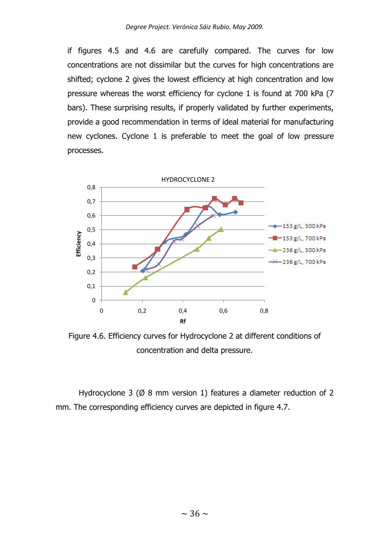
Figure 4.6 illustrates the efficiency curves for hydrocyclone 2 (20% PTFE, Ø
10 mm). The only difference between this cyclone and the first one is the
material used in its construction; cyclone 1 is made of plastic PA66 whereas
cyclone 2 has been constructed with plastic PA66 plus a 20% of PTFE. Being
the material the only difference, we might expect a similar behavior, but
results show that the responses of both cyclones are quite different, as seen
0
0,1
0,2
0,3
0,4
0,5
0,6
0,7
0,8
0,9
0 0,2 0,4 0,6 0,8
Effi
cie
ncy
Rf
HYDROCYCLONE 1
153 g/L, 500 kPa
153 g/L, 700 kPa
236 g/L, 500 kPa
236 g/L, 700 kPa
Degree Project. Verónica Sáiz Rubio. May 2009.
~ 36 ~
if figures 4.5 and 4.6 are carefully compared. The curves for low
concentrations are not dissimilar but the curves for high concentrations are
shifted; cyclone 2 gives the lowest efficiency at high concentration and low
pressure whereas the worst efficiency for cyclone 1 is found at 700 kPa (7
bars). These surprising results, if properly validated by further experiments,
provide a good recommendation in terms of ideal material for manufacturing
new cyclones. Cyclone 1 is preferable to meet the goal of low pressure
processes.
Figure 4.6. Efficiency curves for Hydrocyclone 2 at different conditions of
concentration and delta pressure.
Hydrocyclone 3 (Ø 8 mm version 1) features a diameter reduction of 2
mm. The corresponding efficiency curves are depicted in figure 4.7.
0
0,1
0,2
0,3
0,4
0,5
0,6
0,7
0,8
0 0,2 0,4 0,6 0,8
Effi
cie
ncy
Rf
HYDROCYCLONE 2
Degree Project. Verónica Sáiz Rubio. May 2009.
~ 37 ~
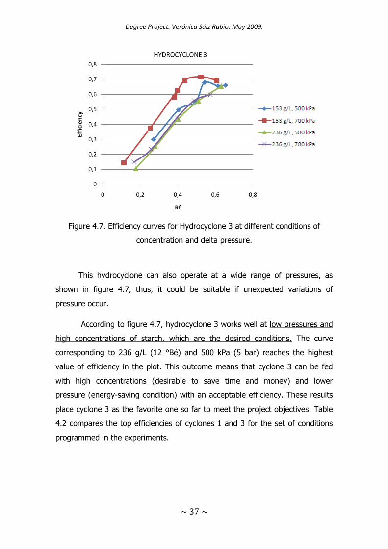
Figure 4.7. Efficiency curves for Hydrocyclone 3 at different conditions of
concentration and delta pressure.
This hydrocyclone can also operate at a wide range of pressures, as
shown in figure 4.7, thus, it could be suitable if unexpected variations of
pressure occur.
According to figure 4.7, hydrocyclone 3 works well at low pressures and
high concentrations of starch, which are the desired conditions. The curve
corresponding to 236 g/L (12 °Bé) and 500 kPa (5 bar) reaches the highest
value of efficiency in the plot. This outcome means that cyclone 3 can be fed
with high concentrations (desirable to save time and money) and lower
pressure (energy-saving condition) with an acceptable efficiency. These results
place cyclone 3 as the favorite one so far to meet the project objectives. Table
4.2 compares the top efficiencies of cyclones 1 and 3 for the set of conditions
programmed in the experiments.
0
0,1
0,2
0,3
0,4
0,5
0,6
0,7
0,8
0 0,2 0,4 0,6 0,8
Effi
cie
ncy
Rf
HYDROCYCLONE 3
Degree Project. Verónica Sáiz Rubio. May 2009.
~ 38 ~
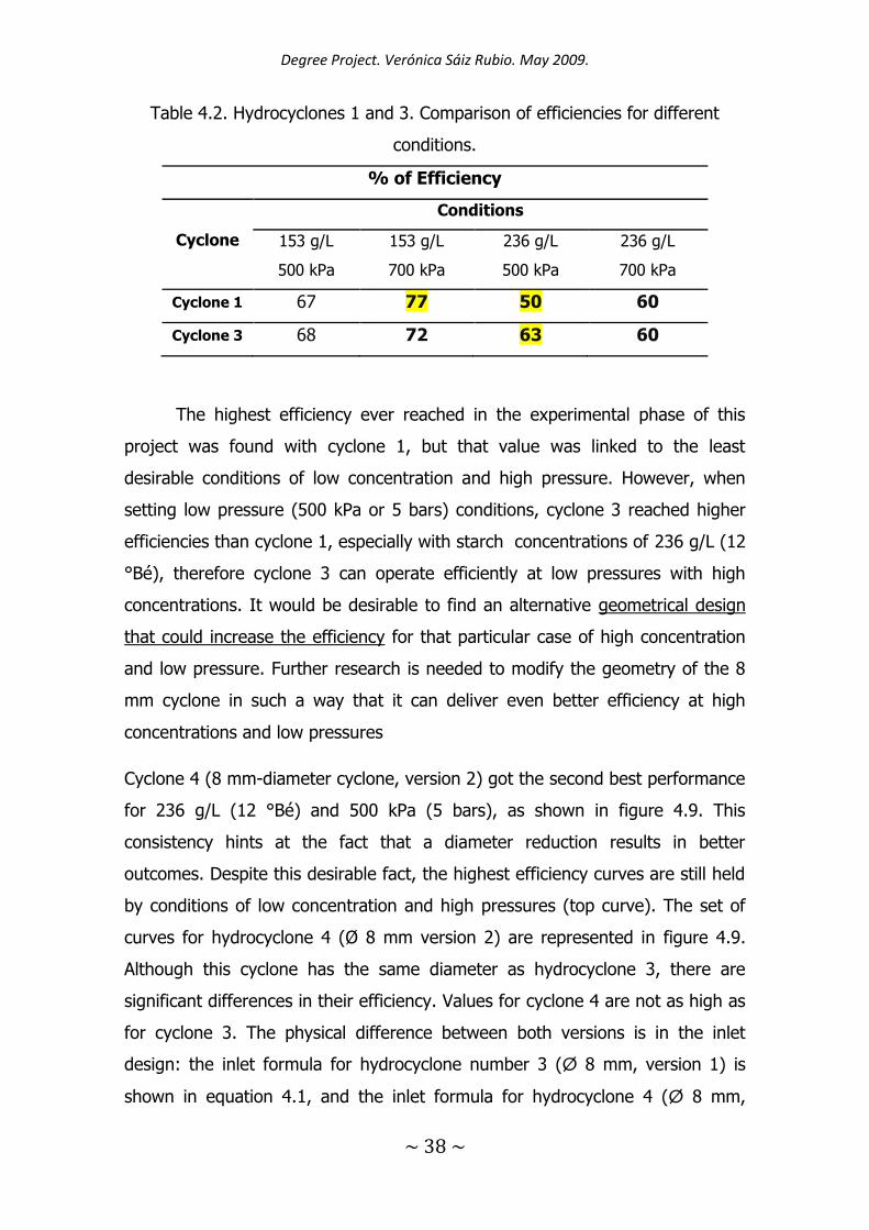
Table 4.2. Hydrocyclones 1 and 3. Comparison of efficiencies for different
conditions.
% of Efficiency
Cyclone
Conditions
153 g/L
500 kPa
153 g/L
700 kPa
236 g/L
500 kPa
236 g/L
700 kPa
Cyclone 1 67 77 50 60
Cyclone 3 68 72 63 60
The highest efficiency ever reached in the experimental phase of this
project was found with cyclone 1, but that value was linked to the least
desirable conditions of low concentration and high pressure. However, when
setting low pressure (500 kPa or 5 bars) conditions, cyclone 3 reached higher
efficiencies than cyclone 1, especially with starch concentrations of 236 g/L (12
°Bé), therefore cyclone 3 can operate efficiently at low pressures with high
concentrations. It would be desirable to find an alternative geometrical design
that could increase the efficiency for that particular case of high concentration
and low pressure. Further research is needed to modify the geometry of the 8
mm cyclone in such a way that it can deliver even better efficiency at high
concentrations and low pressures
Cyclone 4 (8 mm-diameter cyclone, version 2) got the second best performance
for 236 g/L (12 °Bé) and 500 kPa (5 bars), as shown in figure 4.9. This
consistency hints at the fact that a diameter reduction results in better
outcomes. Despite this desirable fact, the highest efficiency curves are still held
by conditions of low concentration and high pressures (top curve). The set of
curves for hydrocyclone 4 (Ø 8 mm version 2) are represented in figure 4.9.
Although this cyclone has the same diameter as hydrocyclone 3, there are
significant differences in their efficiency. Values for cyclone 4 are not as high as
for cyclone 3. The physical difference between both versions is in the inlet
design: the inlet formula for hydrocyclone number 3 (Ø 8 mm, version 1) is
shown in equation 4.1, and the inlet formula for hydrocyclone 4 (Ø 8 mm,
Degree Project. Verónica Sáiz Rubio. May 2009.
~ 39 ~
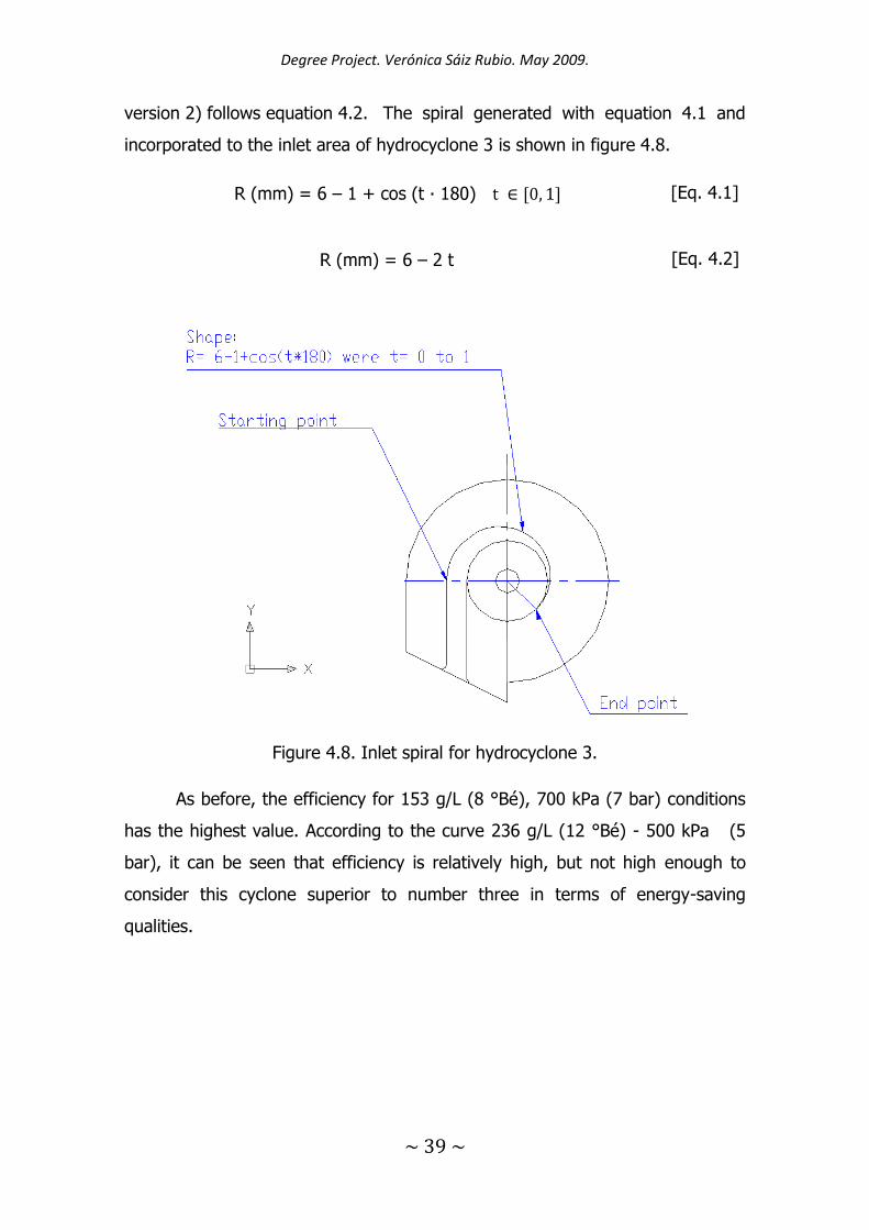
version 2) follows equation 4.2. The spiral generated with equation 4.1 and
incorporated to the inlet area of hydrocyclone 3 is shown in figure 4.8.
– [Eq. 4.1]
– [Eq. 4.2]
Figure 4.8. Inlet spiral for hydrocyclone 3.
As before, the efficiency for 153 g/L (8 °Bé), 700 kPa (7 bar) conditions
has the highest value. According to the curve 236 g/L (12 °Bé) - 500 kPa (5
bar), it can be seen that efficiency is relatively high, but not high enough to
consider this cyclone superior to number three in terms of energy-saving
qualities.
Degree Project. Verónica Sáiz Rubio. May 2009.
~ 40 ~
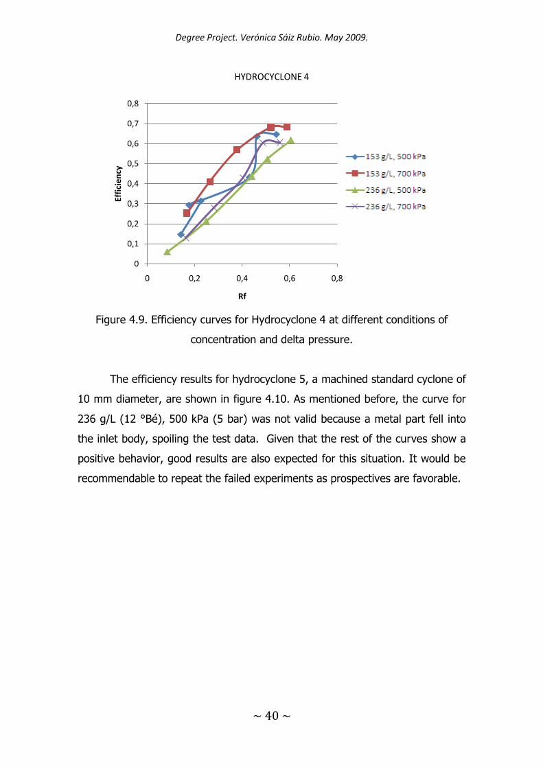
Figure 4.9. Efficiency curves for Hydrocyclone 4 at different conditions of
concentration and delta pressure.
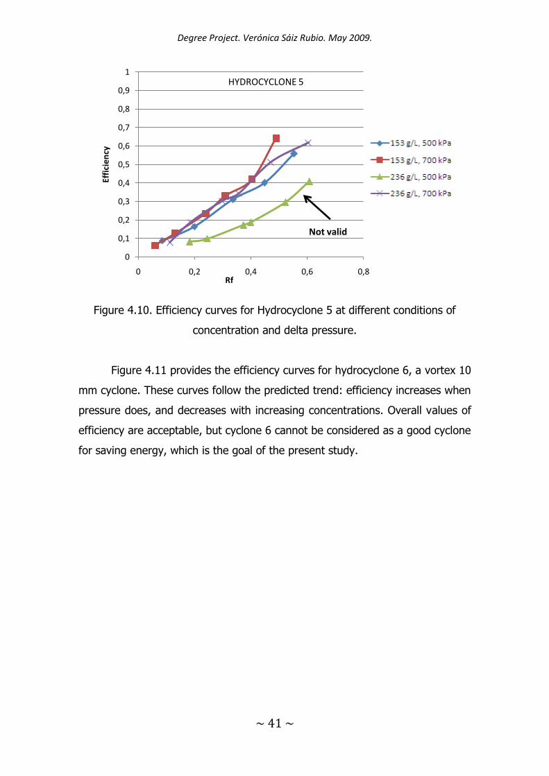
The efficiency results for hydrocyclone 5, a machined standard cyclone of
10 mm diameter, are shown in figure 4.10. As mentioned before, the curve for
236 g/L (12 °Bé), 500 kPa (5 bar) was not valid because a metal part fell into
the inlet body, spoiling the test data. Given that the rest of the curves show a
positive behavior, good results are also expected for this situation. It would be
recommendable to repeat the failed experiments as prospectives are favorable.
0
0,1
0,2
0,3
0,4
0,5
0,6
0,7
0,8
0 0,2 0,4 0,6 0,8
Effi
cie
ncy
Rf
HYDROCYCLONE 4
Degree Project. Verónica Sáiz Rubio. May 2009.
~ 41 ~
Figure 4.10. Efficiency curves for Hydrocyclone 5 at different conditions of
concentration and delta pressure.
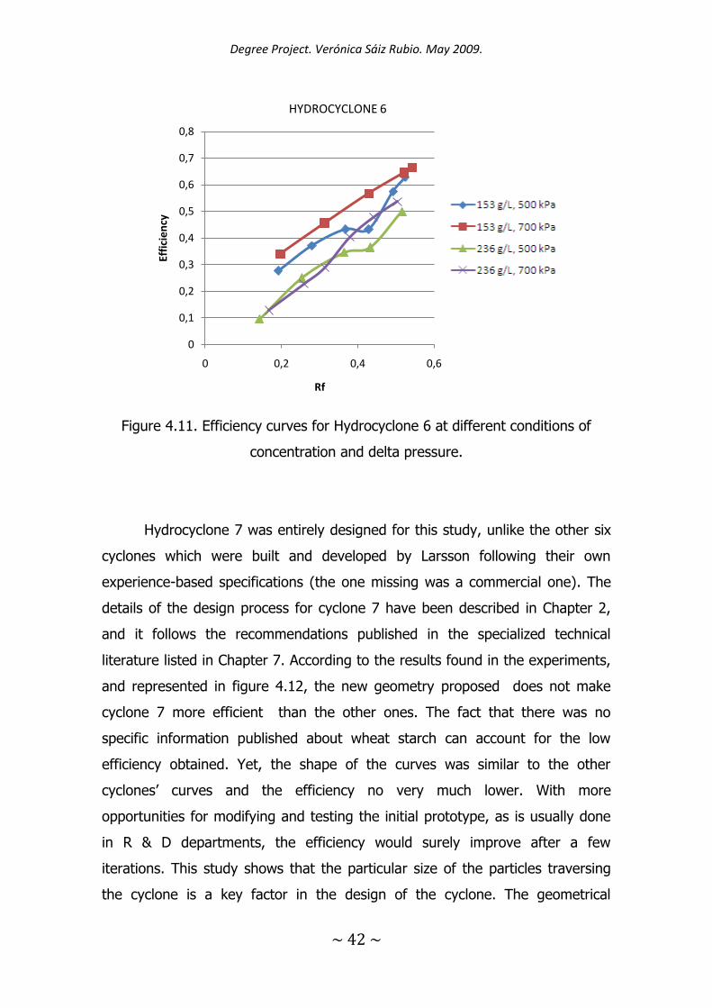
Figure 4.11 provides the efficiency curves for hydrocyclone 6, a vortex 10
mm cyclone. These curves follow the predicted trend: efficiency increases when
pressure does, and decreases with increasing concentrations. Overall values of
efficiency are acceptable, but cyclone 6 cannot be considered as a good cyclone
for saving energy, which is the goal of the present study.
0
0,1
0,2
0,3
0,4
0,5
0,6
0,7
0,8
0,9
1
0 0,2 0,4 0,6 0,8
Effi
cie
ncy
Rf
HYDROCYCLONE 5
Not valid
Degree Project. Verónica Sáiz Rubio. May 2009.
~ 42 ~
Figure 4.11. Efficiency curves for Hydrocyclone 6 at different conditions of
concentration and delta pressure.
Hydrocyclone 7 was entirely designed for this study, unlike the other six
cyclones which were built and developed by Larsson following their own
experience-based specifications (the one missing was a commercial one). The
details of the design process for cyclone 7 have been described in Chapter 2,
and it follows the recommendations published in the specialized technical
literature listed in Chapter 7. According to the results found in the experiments,
and represented in figure 4.12, the new geometry proposed does not make
cyclone 7 more efficient than the other ones. The fact that there was no
specific information published about wheat starch can account for the low
efficiency obtained. Yet, the shape of the curves was similar to the other
cyclones’ curves and the efficiency no very much lower. With more
opportunities for modifying and testing the initial prototype, as is usually done
in R & D departments, the efficiency would surely improve after a few
iterations. This study shows that the particular size of the particles traversing
the cyclone is a key factor in the design of the cyclone. The geometrical
0
0,1
0,2
0,3
0,4
0,5
0,6
0,7
0,8
0 0,2 0,4 0,6
Effi
cie
ncy
Rf
HYDROCYCLONE 6
Degree Project. Verónica Sáiz Rubio. May 2009.
~ 43 ~
properties of hydrocyclones cannot be the same for potato starch, tapioca
starch or wheat starch.
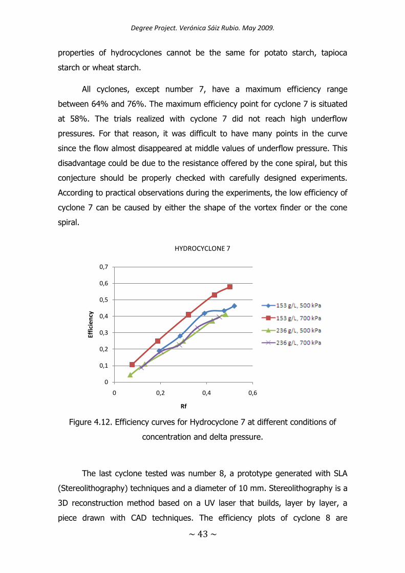
All cyclones, except number 7, have a maximum efficiency range
between 64% and 76%. The maximum efficiency point for cyclone 7 is situated
at 58%. The trials realized with cyclone 7 did not reach high underflow
pressures. For that reason, it was difficult to have many points in the curve
since the flow almost disappeared at middle values of underflow pressure. This
disadvantage could be due to the resistance offered by the cone spiral, but this
conjecture should be properly checked with carefully designed experiments.
According to practical observations during the experiments, the low efficiency of
cyclone 7 can be caused by either the shape of the vortex finder or the cone
spiral.
Figure 4.12. Efficiency curves for Hydrocyclone 7 at different conditions of
concentration and delta pressure.
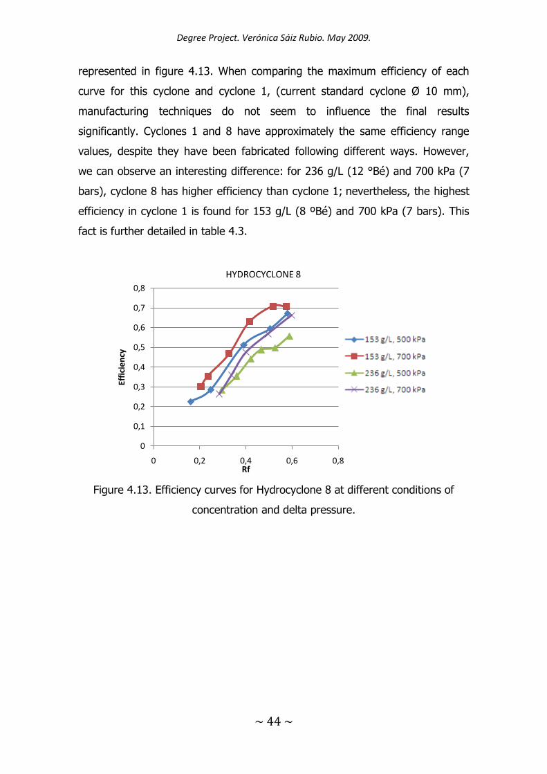
The last cyclone tested was number 8, a prototype generated with SLA
(Stereolithography) techniques and a diameter of 10 mm. Stereolithography is a
3D reconstruction method based on a UV laser that builds, layer by layer, a
piece drawn with CAD techniques. The efficiency plots of cyclone 8 are
0
0,1
0,2
0,3
0,4
0,5
0,6
0,7
0 0,2 0,4 0,6
Effi
cie
ncy
Rf
HYDROCYCLONE 7
Degree Project. Verónica Sáiz Rubio. May 2009.
~ 44 ~
represented in figure 4.13. When comparing the maximum efficiency of each
curve for this cyclone and cyclone 1, (current standard cyclone Ø 10 mm),
manufacturing techniques do not seem to influence the final results
significantly. Cyclones 1 and 8 have approximately the same efficiency range
values, despite they have been fabricated following different ways. However,
we can observe an interesting difference: for 236 g/L (12 °Bé) and 700 kPa (7
bars), cyclone 8 has higher efficiency than cyclone 1; nevertheless, the highest
efficiency in cyclone 1 is found for 153 g/L (8 ºBé) and 700 kPa (7 bars). This
fact is further detailed in table 4.3.
Figure 4.13. Efficiency curves for Hydrocyclone 8 at different conditions of
concentration and delta pressure.
0
0,1
0,2
0,3
0,4
0,5
0,6
0,7
0,8
0 0,2 0,4 0,6 0,8
Effi
cie
ncy
Rf
HYDROCYCLONE 8
Degree Project. Verónica Sáiz Rubio. May 2009.
~ 45 ~
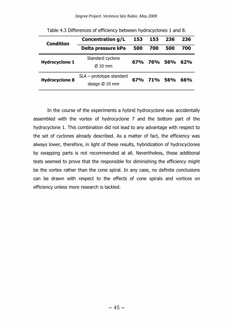
Table 4.3 Differences of efficiency between hydrocyclones 1 and 8.
Condition Concentration g/L 153 153 236 236
Delta pressure kPa 500 700 500 700
Hydrocyclone 1 Standard cyclone
Ø 10 mm 67% 76% 56% 62%
Hydrocyclone 8 SLA – prototype standard
design Ø 10 mm 67% 71% 56% 66%
In the course of the experiments a hybrid hydrocyclone was accidentally
assembled with the vortex of hydrocyclone 7 and the bottom part of the
hydrocyclone 1. This combination did not lead to any advantage with respect to
the set of cyclones already described. As a matter of fact, the efficiency was
always lower, therefore, in light of these results, hybridization of hydrocyclones
by swapping parts is not recommended at all. Nevertheless, these additional
tests seemed to prove that the responsible for diminishing the efficiency might
be the vortex rather than the cone spiral. In any case, no definite conclusions
can be drawn with respect to the effects of cone spirals and vortices on
efficiency unless more research is tackled.
Degree Project. Verónica Sáiz Rubio. May 2009.
~ 46 ~
Chapter 5
Conclusions
The main objective of this project was the improvement of hydrocyclone
efficiency for wheat starch separation, and this overall goal has been reached.
There is a hydrocyclone, out of the eight tested, that clearly meets the
requirements to be considered an energy-saving hydrocyclone. This cyclone is
the 8 mm cyclone (version 1) manufactured by Larsson Company. It worked
better, not only for the desired pressure condition of 500 kPa, but also for the
optimum combination of pressure and concentration given by 236 g/l and 500
kPa.
The Larsson Hydrocyclone version 2, also with a diameter of 8 mm, has
the second highest efficiency for the desired combination of pressure and
concentration. The standard 10 mm Larsson hydrocyclone is near the best
efficiencies for the desired conditions and reaches the top efficiency for a
pressure of 700 kPa and a concentration of 153. The 8 mm cyclone which
yielded the best results was obtained by modifying this 10 mm version.
Another hydrocyclone evaluated in this project was the standard 10 mm
Larsson cyclone, but manufactured applying Rapid Prototyping Stereolitography
(SLA) techniques. This model had values of efficiency that were lower than
those found for the standard 10 mm hydrocyclone It seems that, according to
experimental observations, the way of manufacturing hydrocyclones directly
affects efficiency values, but definite conclusions cannot be drawn until more
research is done.
The geometry-based hydrocyclone designed and developed over this
project had low efficiency and could not operate favorably for a wide range of
underflow pressures. The apparent reason for this outcome might be in the
introduction of too many geometrical variations in one single cyclone, which
complicates the discrimination of the individual effect of each parameter on the
Degree Project. Verónica Sáiz Rubio. May 2009.
~ 47 ~
final efficiency value. A better approach could have been followed by modifying
the prototype step by step while registering the efficiency after each
modification made. The only reason for not proceeding in that way is the
scarcity of time for testing at a remote facility. The scheduled time for
conducting all the experiments was one week, and some time was needed to
check the testing bench. Despite the low efficiency values found for this
hydrocyclone, it cannot be assured that these innovative modifications are not
beneficial because if they had been individually evaluated, a more realistic
assessment would have probably been realized. Therefore, the presence of a
spiral in the conical part of the cyclone, the decrease of the overflow diameter,
and the extension of the vortex finder length seem to be positive modifications
to raise efficiency.
Not much research has been published on the enhancement of efficiency
in wheat starch separation processes. The specific conclusions drawn from the
tests performed on the geometry-based cyclone proposed and designed in this
project are the following:
The recommended prototype hydrocyclone should be tried without the
spiral carved on its conical part because this element can increase the
resistance to flow and, contrarily to what has been suggested by
Svarovsky (1984), it might decrease the efficiency of the cyclone.
Improvements are to be expected if the cyclone incorporates a different
vortex. The current one introduced a significant change compared to
those showing better efficiency values. In particular, it should be tried
with a shorter vortex finder and with a smaller overflow diameter.
The introduction of a central part in the hydrocyclone’s body to avoid the
turbulences created by rough rotational flows produced when the feed
enters tangentially will probably enhance efficiency although it involves a
more sophisticated design. In fact, Chu et al. (2000) found that the
insertion of a central part on a cyclone was the most significant
parameter on the energy loss coefficient.

Degree Project. Verónica Sáiz Rubio. May 2009.
~ 48 ~
The influence of the average particle size on the hydrocyclone design still
remains an unknown factor, which should be carefully studied in the
future.
This interesting research opened several paths for further investigations. In
particular, next steps could be taken in the following directions:
Enhancement of the efficiencies of those hydrocyclones that gave the
best results in the trials by slightly changing the geometry of the cyclone,
especially for version 1 cyclone of 8 mm, , which has very promising
features.
Study if the way of manufacturing cyclones has a notable influence on
efficiency values. If the correlation is negative, hydrocyclones could be
manufactured using rapid-prototyping techniques, with the consequent
savings of manufacturing costs.
Sequential testing of all the geometric modifications proposed by Chu et
al. (2000) in one hydrocyclone model.
Degree Project. Verónica Sáiz Rubio. May 2009.
~ 49 ~
Chapter 6
Acknowledgements
I would like to thank Larsson M. Verkstad AB, and especially Jonas
Oskarsson and Thomas Johansson, for allowing me to carry out this research
project and have a wonderful industry experience for my degree project. I feel
in debt with Professor Samir Khoshaba from the Department of Technology and
Design of Växjö University, who has taken care of all my needs, both personal
and academic, from my very first day in Sweden. I am deeply grateful for all his
assistance and advice. I would also like to express my gratitude to the Erasmus
Program and the Offices of International Programs at Växjö University and the
Polytechnic University of Valencia. Credit needs to be given to my advisor in
Valencia, Francisco Rovira Más, who has been very helpful with technical and
research guidance from the early steps. Finally, it would not be fair to exclude
my family from this section, who have encouraged me to get on board this
adventure, and whose daily support has been crucial for a successful ending.
My most sincere appreciation to all of you.
Degree Project. Verónica Sáiz Rubio. May 2009.
~ 50 ~
Chapter 7
References
Chu, L. Y., J. J. Qin, W. M. Chen, and X. Z. Lee. 2000. Energy consumption and its reduction in the hydrocyclone separation process. III. Effect of the structure of flow field on Energy consumption and energy saving principles. Separation Science and Technology 35 (16): 2679-2705.
Chu, L. Y., W. M. Chen, and X. Z. Lee. 2002a. Effect of structural modification on hydrocyclone performance. Separation and purification technology 21: 71 - 86.
Chu, L. Y., W. M. Chen, and X. Z. Lee. 2002b. Effects of geometric and operating parameters and feed characters on the motion of solid particles in hydrocyclones. Separation and purification technology 26: 237 – 246.
Eliasson, A. C. 2004. Starch in food. Structure, function and applications. Woodhead Publishing, Cambridge, UK.
Emami, S., L.G.Tabil, R.T Tyler and W. Crerar. 2005. Effect of feed concentration and pressure drop in starch-protein. Separation using a hydrocyclone. ASABE Paper No. 056089. St. Joseph, Mich.: ASAE.
Emami, S., L.G. Tabil and R. Tyler. 2006. Isolation of starch and protein from chickpea flour using a hydrocyclone and isoelectric precipitation method. ASABE Paper No. 066090. St. Joseph, Mich.: ASAE.
Fernández Martínez, L., A. Gutiérrez Lavín, M. M. Mahamud, and J. L. Bueno. 2008. Vortex finder optimum length in hydrocyclone separation. Chemical Engineering and Processing 47: 192-199.
Grommers, H.E., J. Krikken, B. H. Bos, and D.A. van der Krogt. 2004. Comparison of small hydrocyclones based on total process costs. Minerals Engineering 17: 581-589.
Gupta, R., M.D. Kaulaskar, V. Kumar, R. Sripriya, B. C. Meikap, and S. Chakraborty. 2008. Studies on the understanding mechanism of air core and vortex formation in a hydrocyclone. Chemical Engineering Journal 144: 153 - 166.
Habibian, M., M. Pazouki, H. Ghanaie, and K. Abbaspour-Sani. 2008. Application of hydrocyclone for removal of yeasts from alcohol fermentations broth. Chemical Engineering Journal 138: 30-34.
Saengchan, K., A. Nopharatana, and W. Songkasiri. 2009. Enhancement of apex diameter, feed concentration and pressure drop on tapioca starch separation with a hydrocyclone. Chemical Engineering and Processing 48: 195-202.
Svarovsky, L. 1984. Hydrocyclones. Holt, Rinehart and Winston Ltd., London, UK.
Degree Project. Verónica Sáiz Rubio. May 2009.
~ 51 ~
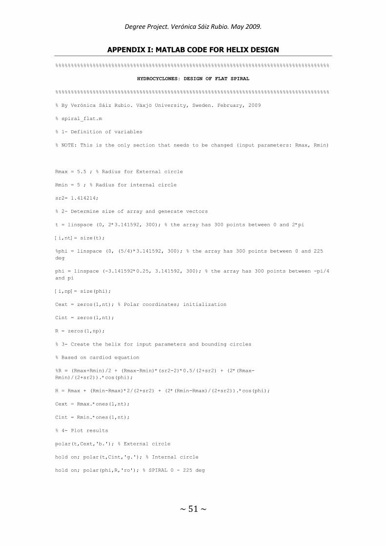
APPENDIX I: MATLAB CODE FOR HELIX DESIGN
%%%%%%%%%%%%%%%%%%%%%%%%%%%%%%%%%%%%%%%%%%%%%%%%%%%%%%%%%%%%%%%%%%%%%%%%%%%%%%%%%%%%%%%%
HYDROCYCLONES: DESIGN OF FLAT SPIRAL
%%%%%%%%%%%%%%%%%%%%%%%%%%%%%%%%%%%%%%%%%%%%%%%%%%%%%%%%%%%%%%%%%%%%%%%%%%%%%%%%%%%%%%%%
% By Verónica Sáiz Rubio. Växjö University, Sweden. February, 2009
% spiral_flat.m
% 1- Definition of variables
% NOTE: This is the only section that needs to be changed (input parameters: Rmax, Rmin)
Rmax = 5.5 ; % Radius for External circle
Rmin = 5 ; % Radius for internal circle
sr2= 1.414214;
% 2- Determine size of array and generate vectors
t = linspace (0, 2*3.141592, 300); % the array has 300 points between 0 and 2*pi
[i,nt]= size(t);
%phi = linspace (0, (5/4)*3.141592, 300); % the array has 300 points between 0 and 225
deg
phi = linspace (-3.141592*0.25, 3.141592, 300); % the array has 300 points between -pi/4
and pi
[i,np]= size(phi);
Cext = zeros(1,nt); % Polar coordinates; initialization
Cint = zeros(1,nt);
R = zeros(1,np);
% 3- Create the helix for input parameters and bounding circles
% Based on cardiod equation
%R = (Rmax+Rmin)/2 + (Rmax-Rmin)*(sr2-2)*0.5/(2+sr2) + (2*(Rmax-
Rmin)/(2+sr2)).*cos(phi);
R = Rmax + (Rmin-Rmax)*2/(2+sr2) + (2*(Rmin-Rmax)/(2+sr2)).*cos(phi);
Cext = Rmax.*ones(1,nt);
Cint = Rmin.*ones(1,nt);
% 4- Plot results
polar(t,Cext,'b.'); % External circle
hold on; polar(t,Cint,'g.'); % Internal circle
hold on; polar(phi,R,'ro'); % SPIRAL 0 - 225 deg

Degree Project. Verónica Sáiz Rubio. May 2009.
~ 52 ~
APPENDIX II: MATLAB CODE FOR HELIX DESIGN
%%%%%%%%%%%%%%%%%%%%%%%%%%%%%%%%%%%%%%%%%%%%%%%%%%%%%%%%%%%%%%%%%%%%%%%%%%%%%%%%%%
HYDROCYCLONES: DESIGN OF SPIRAL [conical helix]
%%%%%%%%%%%%%%%%%%%%%%%%%%%%%%%%%%%%%%%%%%%%%%%%%%%%%%%%%%%%%%%%%%%%%%%%%%%%%%%%%%%%%%%%
% By Verónica Sáiz Rubio. Växjö University, Sweden. February, 2009
% 1- Definition of variables
% NOTE: This is the only section that needs to be changed (input parameters: Rmax, Rmin,
L, Le)
Rmax = 5 ; % Radius in mm of wide section of the cone
Rmin = 1.5 ; % Radius in mm of narrow (output) section of the cone
L = 57 ; % Length of cone, always in mm
Le = 5 ; % helix pitch in mm
% 2- Determine size of array and generate parametric vector t
n = floor(L/Le); %number of loops
t = linspace (0, floor(n*2*3.141592), 300) % the parametric array has 300 points between
0 and 2*pi*n
[i,nt]= size(t)
x = zeros(1,nt); % Cartesian coordinates in mm and 3D space, array of size [2*pi*n,1];
initialization
y = zeros(1,nt); z = zeros(1,nt);
% 3- Create the helix for input parameters
% Parametric equations with Cartesian coordinates
z = (Le/6.283185)*t;
x = (Rmin + (Rmax-Rmin).*(L-z)/L).*cos(t);
y = (Rmin + (Rmax-Rmin).*(L-z)/L).*sin(t);
% 4- Plot results
plot3(x,y,z, 'r-'); % 3D visualization of helix
xlabel ('X [mm]'); ylabel ('Y [mm]'); zlabel ('Z [mm]');
title ('Conical helix for experimental hydrocyclone');
figure; plot3(x,y,z, 'm-'); % Front view of helix
xlabel ('X [mm]'); ylabel ('Y [mm]');
title ('Front view of Conical helix'); view (0,90);
figure; plot3(x,y,z, 'b-'); % Front view of helix
xlabel ('X [mm]'); ylabel ('Y [mm]');
title ('Lateral view of Conical helix'); view (90,0);


![Leaching of amylose from wheat and corn starch · Q-^^ AllEOfi31Sfl3E]](https://img.pdfslide.us/doc/110x75/5e83b0df0da5934e304d5a7c/leaching-of-amylose-from-wheat-and-corn-starch-q-alleofi31sfl3e.jpg)