Design of a Microfluidic Device for the Analysis ofBiofilm Behavior in a Microbial Fuel Cell

by

A-Andrew D. Jones, III

S.B., Department of Mathematics, Massachusetts Institute ofTechnology (2010)

S.B., Department of Mechanical Engineering, Massachusetts Institute ofTechnology (2010)

Submitted to the Department of Mechanical Engineeringin partial fulfillment of the requirements for the degree of

Masters of Science in Mechanical Engineering

at the

MASSACHUSETTS INSTITUTE OF TECHNOLOGY

February 2014

c© Massachusetts Institute of Technology 2014. All rights reserved.

Author . . . . . . . . . . . . . . . . . . . . . . . . . . . . . . . . . . . . . . . . . . . . . . . . . . . . . . . . . . . . . . . .Department of Mechanical Engineering

January 18, 2014

Certified by. . . . . . . . . . . . . . . . . . . . . . . . . . . . . . . . . . . . . . . . . . . . . . . . . . . . . . . . . . . .Cullen R. Buie

Assistant Professor of Mechanical EngineeringThesis Supervisor

Accepted by . . . . . . . . . . . . . . . . . . . . . . . . . . . . . . . . . . . . . . . . . . . . . . . . . . . . . . . . . . .David E. Hardt

Ralph E. and Eloise F. Cross Professor of Mechanical EngineeringChairman, Department Committee on Graduate Theses

2

Design of a Microfluidic Device for the Analysis of Biofilm

Behavior in a Microbial Fuel Cell

by

A-Andrew D. Jones, III

Submitted to the Department of Mechanical Engineeringon January 18, 2014, in partial fulfillment of the

requirements for the degree ofMasters of Science in Mechanical Engineering

Abstract

This thesis presents design, manufacturing, testing, and modeling of a laminar-flowmicrobial fuel cell. Novel means were developed to use graphite and other bulk-scalematerials in a microscale device without loosing any properties of the bulk material.Micro-milling techniques were optimized for use on acrylic to achieve surface rough-ness averages as low as Ra = 100 nm for a 55µm deep cut. Power densities as highas 0.4 mW ·m−2, (28 mV at open circuit) in the first ever polarization curve for alaminar-flow microbial fuel cell. A model was developed for biofilm behavior incor-porating shear and pore pressure as mechanisms for biofilm loss. The model agreeswith experimental observations on fluid flow through biofilms, biofilm structure, andother biofilm loss events.

Thesis Supervisor: Cullen R. BuieTitle: Assistant Professor of Mechanical Engineering

3

4

Acknowledgments

I would like to acknowledge my advisor, Professor Cullen R. Buie and all the

members of the MIT Laboratory for Energy & Microsystems Innovation. I would like

to thank the Lemelson Foundation for funding my first year of work. I would like to

thank the MIT Microsystems Technology Lab and Research Associate Kurt Broderick

for the assistance in design, manufacturing, and characterization of the electrodes

and devices. I would like to thank Professor Martin L. Culpepper and his Precision

Compliant Systems Lab for the use and help using the micromill. I would like to

thank the MIT Center for Materials Science and Engineering and Research Associate’s

Patrick Boisvert and Libby Shaw for help with AFM imaging and SEM imaging. I

would like to thank Dr. Valerie Watson and the Keck Center for Microscopy in

the Whitehead Institute for Biomedical Research for tips and tricks for drying and

imaging biofilms.

I would like to acknowledge my wife, Cristen Blair Jones for her love, support,

and multiple photoshop edits and illustrator wizardry. I would like to acknowledge

my parents Andrew D. and Julie L. Jones for my birth, their love, support, and

comments. I would also like to acknowledge my sisters Khoranhalai Juliealma Lyki’El

Melba Jones and Khoranalai Anjulique Josephine Chestina Jones for their love and

support even though I am 500 mi away.

5

THIS PAGE INTENTIONALLY LEFT BLANK

6

Contents

1 Introduction 13

1.1 Fundamentals of biofilm dynamics . . . . . . . . . . . . . . . . . . . . 13

1.2 The Importance of Biofilms . . . . . . . . . . . . . . . . . . . . . . . 16

1.2.1 Energy - Water Nexus . . . . . . . . . . . . . . . . . . . . . . 16

1.2.2 Microbial Induced Corrosion . . . . . . . . . . . . . . . . . . . 19

1.2.3 Medical Biofilms . . . . . . . . . . . . . . . . . . . . . . . . . 20

1.3 Methods for studying biofilms . . . . . . . . . . . . . . . . . . . . . . 21

1.4 Present models of biofilm dynamics . . . . . . . . . . . . . . . . . . . 23

1.4.1 Growth . . . . . . . . . . . . . . . . . . . . . . . . . . . . . . 23

1.4.2 Detachment . . . . . . . . . . . . . . . . . . . . . . . . . . . . 24

1.4.3 Structure . . . . . . . . . . . . . . . . . . . . . . . . . . . . . 26

1.4.4 Bioelectrochemistry . . . . . . . . . . . . . . . . . . . . . . . . 27

1.5 Thesis summary . . . . . . . . . . . . . . . . . . . . . . . . . . . . . . 29

2 Methods for studying biofilms 31

2.1 Microfluidics . . . . . . . . . . . . . . . . . . . . . . . . . . . . . . . . 31

2.2 Design, Manufacturing, and Materials . . . . . . . . . . . . . . . . . 32

2.2.1 Design . . . . . . . . . . . . . . . . . . . . . . . . . . . . . . . 32

2.2.2 Manufacturing . . . . . . . . . . . . . . . . . . . . . . . . . . 41

2.2.3 Materials . . . . . . . . . . . . . . . . . . . . . . . . . . . . . 45

2.3 Testing . . . . . . . . . . . . . . . . . . . . . . . . . . . . . . . . . . . 49

2.4 Modeling biofilm dynamics . . . . . . . . . . . . . . . . . . . . . . . . 53

2.4.1 Fluid Flow . . . . . . . . . . . . . . . . . . . . . . . . . . . . . 54

7

2.4.2 Solute Advection - Diffusion - Reaction . . . . . . . . . . . . . 56

2.4.3 Biofilm evolution . . . . . . . . . . . . . . . . . . . . . . . . . 59

2.4.4 Bioelectrochemistry . . . . . . . . . . . . . . . . . . . . . . . . 61

2.4.5 Model Summary . . . . . . . . . . . . . . . . . . . . . . . . . 62

3 Results & Discussion 67

4 Conclusion & Future Work 79

A Machinist Parameters for a Laminar Flow - Microbial Fuel Cell 81

8

List of Figures

1-1 An illustration of transport through an electroactive biofilm . . . . . 14

1-2 Biofilm grown on carbon paper in a microbial fuel cell . . . . . . . . . 17

1-3 Survey of power density (by area) versus anode material type . . . . 18

2-1 Simulation of Laminar Flow - Microbial Fuel Cell Channels . . . . . . 33

2-2 Simulation of Laminar Flow - Microbial Fuel Cell Channels . . . . . . 34

2-3 Laminar-Flow Microbial Fuel Cell from PDMS . . . . . . . . . . . . . 35

2-4 Sputter Deposition of Carbon on Gold . . . . . . . . . . . . . . . . . 37

2-5 Carbon Black in PDMS . . . . . . . . . . . . . . . . . . . . . . . . . 38

2-6 Microchip Laminar Flow -Microbial Fuel Cell . . . . . . . . . . . . . 39

2-7 Interchangeable electrodes . . . . . . . . . . . . . . . . . . . . . . . . 40

2-8 Representative Surface Roughness . . . . . . . . . . . . . . . . . . . . 43

2-9 Polished acrylic . . . . . . . . . . . . . . . . . . . . . . . . . . . . . . 44

2-10 Images of the electrodes taken at scale of 4:1 and 5:1 . . . . . . . . . 46

2-11 Images of the electrodes taken at scale of 4:1 and 5:1 . . . . . . . . . 47

2-12 Gibbs Free Energy of interaction . . . . . . . . . . . . . . . . . . . . 50

2-13 LF-MFC Schematic . . . . . . . . . . . . . . . . . . . . . . . . . . . . 51

2-14 Cyclic-Voltamogram for the LF-MFC with PYG without bacteria . . 52

3-1 Potentiostatic Electrochemical Impedance Spectroscopy for the LF-

MFC with PYG without bacteria . . . . . . . . . . . . . . . . . . . . 68

3-2 Potentiostatic Electrochemical Impedance Spectroscopy for the LF-

MFC with PYG . . . . . . . . . . . . . . . . . . . . . . . . . . . . . 69

3-3 Polarization Curve of an LF-MFC . . . . . . . . . . . . . . . . . . . . 70

9

3-4 Voltage versus time of an LF-MFC . . . . . . . . . . . . . . . . . . . 71

3-5 Polarization Curve of an MFC . . . . . . . . . . . . . . . . . . . . . . 72

3-6 Scanning electron micrograph of biofilm grown on LF-MFC . . . . . . 73

3-7 Simulation of substrate consumption, biofilm growth, and fluid flow . 74

3-8 Biomass density versus height without shear . . . . . . . . . . . . . . 75

3-9 Simulation of substrate consumption, biofilm growth, and fluid flow . 76

3-10 Biomass density versus height with shear . . . . . . . . . . . . . . . . 77

3-11 Exponetial fit of biomass density versus height with and without shear 78

10

List of Tables

1.1 Materials selection for MFC adhesion . . . . . . . . . . . . . . . . . . 19

2.1 Properties of liquids for Surface Energy Calculations . . . . . . . . . 49

2.2 Modeling Parameters . . . . . . . . . . . . . . . . . . . . . . . . . . . 64

2.3 Dimensionless Parameters . . . . . . . . . . . . . . . . . . . . . . . . 65

11

THIS PAGE INTENTIONALLY LEFT BLANK

12

Chapter 1

Introduction

1.1 Fundamentals of biofilm dynamics

A biofilm is a community of bacteria. It is a resilient and robust structure de-

veloped for the protection from external stresses, the pursuit of nutrients, and to

maintain environmental conditions necessary for the population to thrive (cf. Figure

1-1) [82]. When bacteria form biofilms, they are more resistant to antibiotics, preda-

tory bacteria, the immune response of a host, changes in temperature, fluid flow, and

nutrient deficiency. There are metabolic and genetic differences between bacteria in

a biofilm and the same species of bacteria in their nearby planktonic state [82, 54].

Plaque is one of the easiest biofilms to conceptualize. Plaque is gingival and sub-

gingival biofilm formed on teeth. The reason for brushing in a circular motion with

bristles in addition to the use of dilute caustic soda or other chemicals (toothpaste)

is that antibacterial washes alone can not penetrate the biofilm. Subgingival biofilms

attach in many places that the biofilm functions like a composite material in resisting

shear (brushing and flossing) from multiple directions. The biofilms attach on the

roughened surfaces of teeth and branch to cover wide areas. These bacteria are mostly

harmless and potentially beneficial while “swimming” in the mouth but become prob-

lematic when they “customize their living space”. Everything from the chemicals used

to makeup the biofilm to metabolic byproducts begin to become problematic when

they are released in high concentration near the teeth. There are also opportunistic

13

CO2, H+

Fluid Boundary Layer

Concentration Boundary Layer

Flow at porous interface

Flow throughporous media

Electrode

BacterialBio!lm

Acetate

Flow across rough/smooth plate

e- e-

y

z

x

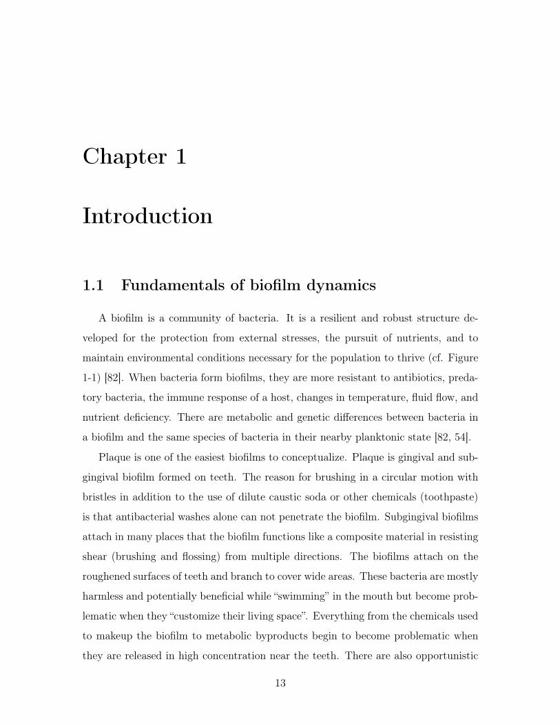
Figure 1-1: An illustration of the transport mechanisms through an electroactivebiofilm. The structure is formed from bacteria and extracellular proteins secretedby the bacteria. The biofilm may entrap structures of the solid support material,like carbon nanotubes, surface roughness, etc. A biofilm regulates the environmen-tal conditions the bacteria are exposed to such as: water content and flux, nutrientflux/storage, secreted regulatory chemicals, like those responsible for quorum sens-ing and antibiotic resistance. From a hydrodynamic perspective, the biofilm is ananisotropic poroelastic media. The porosity in the transverse direction increases ordecreases depending on whether the support is the growth substrate or the substrateis in the fluid. The porosity in the lateral direction is typically greater and not asdepth dependent. From a chemical perspective, the biofilm is an electrochemical cat-alyst and capacitor. Combined, the flow over the biofilm establishes a hydrodynamicand concentration boundary layer above and gradients of pressure and concentrationwithin.

14

bacteria that target tissues and cells like Porphyromonas gingivalis that will attack

young dendritic cells nearby.

Biofilms can incorporate multiple species of bacteria in symbiotic, mutually co-

operative, or exploitative relationships. For example, layers of aerobic bacteria will

form closer to the oxygen rich environments above layers of anaerobic bacteria and

the metabolic byproducts will be shuttled between them. Biofilms made from multi-

ple species of bacteria produce more power than biofilms formed from single species

in microbial fuel cells (cf. Sec. 1.2.1), sometimes by an order of magnitude (Zhang et

al. [93]). Certain species are better at anchoring to a substrate than others providing

a nucleation point of the biofilm.

A biofilm is made from bacterial cells and extracellular polymer substances (EPS)

including: exopolysaccharides like cellulose, proteins and nucleic acids. Biofilms exist

in dry porous media like soil and in bodies of stagnant or moving water[16]. In adverse

fluid flow conditions, biofilms form viscoelastic streamers, where the biofilm is only

anchored at one point and extends into the flow [75, 86]. The viscoelastic properties

of biofilms can sustain a streamer over a centimeter in length. Filamentous biofilms

stretch over centimeter distances to move electrons from anoxic sediment to oxygen

rich surface water [62]. Biofilms are more like vasculated tissue than gelatinous masses

[80]. This vasculature varies in depth and direction and is explored in this thesis [88].

A combination of signaling, quorum sensing, cell-cell signaling, metabolite sensing or

cell death, helps to determine biofilm structure [79].

Biofilms form and maintain existence by many different methods and more meth-

ods are being discovered. Bacteria in biofilms are very different from their planktonic

cousins. They turn on and off up to 10% of their genome, a larger percentage than

could be explained by swimming or sticking [54]. They have complicated commu-

nication methods that are involved in turning on and off EPS production [82, 37].

There are signaling pathways that can cause biofilms to stop formation all together.

Scientist and engineers are trying to exploit the mechanical and biological properties

of biofilms for our benefit.

15

1.2 The Importance of Biofilms

1.2.1 Energy - Water Nexus

The present study on biofilms targets Microbial Fuel Cells as a model plat-

form. Microbial fuel cells have been considered a key component for bridging the

energy/water nexus because of the relationship between biofilms and water treat-

ment. Water treatment consumes over 3% of the total energy consumed in the United

States [2]. This level of energy demand is impossible to meet for the developing world

and is a global problem since inadequate treatment leads to disease and death [56].

Biological treatment is used to remove most organic and some inorganic chemicals in

wastewater whether it is treated in a compost, septic tank, municipal or industrial

wastewater treatment plant [24, 87]. Biological treatment reactors are designed to

produce thin, but not abundant biofilms to expose bacteria to as much of the wastew-

ater as possible for the amount of time required to reduce the pollutant load to safe

limits [24, 39]. Byproducts of these processes include useful methane gas and biomass

that can be turned into fertilizer. Other byproducts are sulfur dioxide, silicon dioxide,

ammonia that limit the use of the synthesized methane as fuel. Microbial fuel cells

are a useful way around this limitation since they produce power directly from the

wastewater.

A microbial fuel cell (MFC) is a device where bacteria consume sugar and other

hydrocarbons and ‘excrete’ CO2, protons and electrons. A typical biofilm formed

during operation of an MFC is shown in Figure 1-2 The electrons travel to corrosion

resistant metals (the anode) while the protons diffuse away from the bacteria to be

combined, at another electrode (the cathode), with the electrons that have passed

through a circuit to generate useful work. MFCs are not a new technology, but

interest in them has shown a resurgence in light of the current energy crises and

UN development goals [69, 5, 56]. Research in the area has achieved power densities

as high as 5 W ·m−2 and continues to increase. Although power densities may not

achieve independence from fossil fuels, they could power a lightbulb so that people

can use the bathroom in places without electricity while simultaneously reducing

16

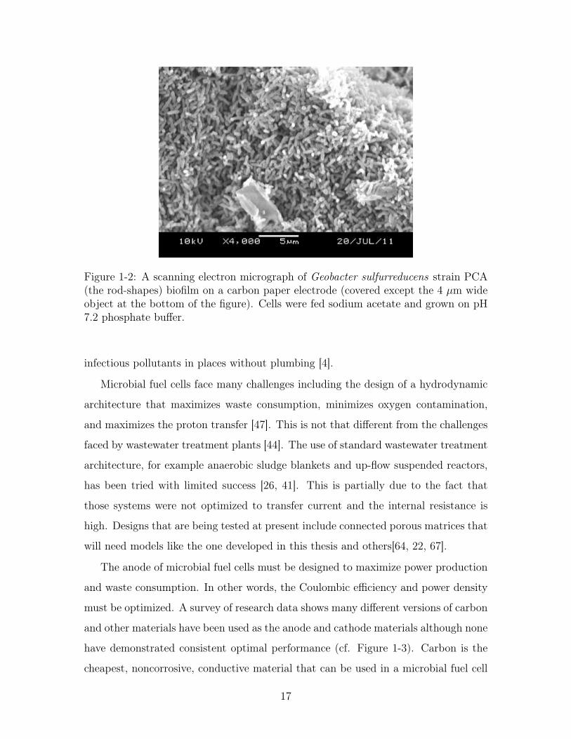
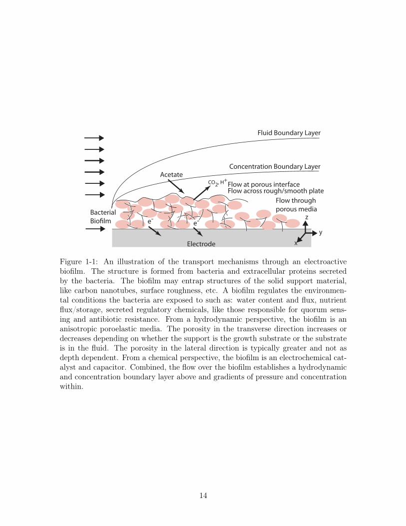
Figure 1-2: A scanning electron micrograph of Geobacter sulfurreducens strain PCA(the rod-shapes) biofilm on a carbon paper electrode (covered except the 4 µm wideobject at the bottom of the figure). Cells were fed sodium acetate and grown on pH7.2 phosphate buffer.

infectious pollutants in places without plumbing [4].

Microbial fuel cells face many challenges including the design of a hydrodynamic

architecture that maximizes waste consumption, minimizes oxygen contamination,

and maximizes the proton transfer [47]. This is not that different from the challenges

faced by wastewater treatment plants [44]. The use of standard wastewater treatment

architecture, for example anaerobic sludge blankets and up-flow suspended reactors,

has been tried with limited success [26, 41]. This is partially due to the fact that

those systems were not optimized to transfer current and the internal resistance is

high. Designs that are being tested at present include connected porous matrices that

will need models like the one developed in this thesis and others[64, 22, 67].

The anode of microbial fuel cells must be designed to maximize power production

and waste consumption. In other words, the Coulombic efficiency and power density

must be optimized. A survey of research data shows many different versions of carbon

and other materials have been used as the anode and cathode materials although none

have demonstrated consistent optimal performance (cf. Figure 1-3). Carbon is the

cheapest, noncorrosive, conductive material that can be used in a microbial fuel cell

17

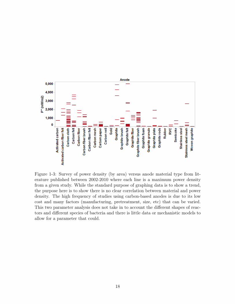
Figure 1-3: Survey of power density (by area) versus anode material type from lit-erature published between 2002-2010 where each line is a maximum power densityfrom a given study. While the standard purpose of graphing data is to show a trend,the purpose here is to show there is no clear correlation between material and powerdensity. The high frequency of studies using carbon-based anodes is due to its lowcost and many factors (manufacturing, pretreatment, size, etc) that can be varied.This two parameter analysis does not take in to account the different shapes of reac-tors and different species of bacteria and there is little data or mechanistic models toallow for a parameter that could.

18

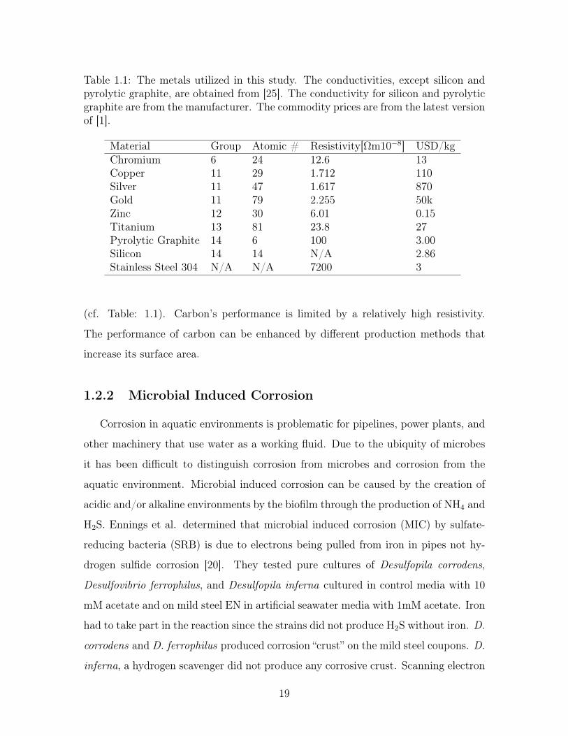
Table 1.1: The metals utilized in this study. The conductivities, except silicon andpyrolytic graphite, are obtained from [25]. The conductivity for silicon and pyrolyticgraphite are from the manufacturer. The commodity prices are from the latest versionof [1].

Material Group Atomic # Resistivity[Ωm10−8] USD/kgChromium 6 24 12.6 13Copper 11 29 1.712 110Silver 11 47 1.617 870Gold 11 79 2.255 50kZinc 12 30 6.01 0.15Titanium 13 81 23.8 27Pyrolytic Graphite 14 6 100 3.00Silicon 14 14 N/A 2.86Stainless Steel 304 N/A N/A 7200 3

(cf. Table: 1.1). Carbon’s performance is limited by a relatively high resistivity.

The performance of carbon can be enhanced by different production methods that

increase its surface area.

1.2.2 Microbial Induced Corrosion

Corrosion in aquatic environments is problematic for pipelines, power plants, and

other machinery that use water as a working fluid. Due to the ubiquity of microbes

it has been difficult to distinguish corrosion from microbes and corrosion from the

aquatic environment. Microbial induced corrosion can be caused by the creation of

acidic and/or alkaline environments by the biofilm through the production of NH4 and

H2S. Ennings et al. determined that microbial induced corrosion (MIC) by sulfate-

reducing bacteria (SRB) is due to electrons being pulled from iron in pipes not hy-

drogen sulfide corrosion [20]. They tested pure cultures of Desulfopila corrodens,

Desulfovibrio ferrophilus, and Desulfopila inferna cultured in control media with 10

mM acetate and on mild steel EN in artificial seawater media with 1mM acetate. Iron

had to take part in the reaction since the strains did not produce H2S without iron. D.

corrodens and D. ferrophilus produced corrosion “crust” on the mild steel coupons. D.

inferna, a hydrogen scavenger did not produce any corrosive crust. Scanning electron

19

micrographs showed crust formation, bacteria colonization (not necessarily a biofilm),

“gas vents” and places of no crust formation. Energy dispersive X-ray spectroscopy

showed that the location of no crust formation was identical to locations of no sulfur.

After 150 days, D corrodens, D ferrophilus, and D inferna had reduced the mild steel

to 27.8%, 68.1% and 98.8% of their original volume respectively. The crust had a

conductivity of ∼ 50 S ·m−1. The reaction rates were faster than what could have

happened during hydrogen sulfide corrosion. The vents appeared to be used for pH

balance, but this was not confirmed experimentally.

1.2.3 Medical Biofilms

1.7 million infections and 99,000 associated deaths occur due to healthcare as-

sociated infections in American hospitals [38]. Biofilms are present in pneumonia,

urinary tract surgical site and blood stream infections that may lead to thrombosis

or sepsis. Biofilms form in several places: on epithelial or endothelial lining, teeth and

implanted medical device (IMD) surfaces; in lung, intestinal or vaginal mucus layers,

and intracellularly [11]. Due to the symbiotic, mutually cooperative, or exploitative

nature of biofilm communities, many of the infectious bacteria are not culturable and

not treatable.

The human immune response to surgery and IMDs can cause greater harm to the

body. The first step in healing injured tissue is the accumulation of platelets and

neutrophils. Macrophages are then recruited by chemical signaling. IMDs, in par-

ticular, are coated with proteins and glycoproteins such as: fibronectin, vitronectin,

fibrinogen, albumin, and immunoglobulins. Bacteria would not be able to attach to

many bioengineered surfaces without this protein coating. Furthermore when exposed

to the host’s immune response (e.g., antibodies) biofilms will grow thicker. Certain

bacteria have even been shown to intentionally recruit host cells in order to start

growing a biofilm.

Specific instances of a biofilm saving bacteria are examples of Pseudomonas aerug-

inosa being saved by its exopolysaccharide alginate matrix from IFN-γ mediated

leukocyte killing[43]. While leukocytes can penetrate Staphylococcus aureus biofilms

20

that are 7-days old when grown in laminar shear, they cannot penetrate 2-day old

biofilms grown in static fluid[42]. Biofilms are not simply benign harborers of hungry

bacteria. Porphyromonas gingivalis produces a specific type of lipopolysaccahrides

that stunts the growth of dendritic cells. Other P. aeruginosa biofilms form “mush-

room explosions” and engulf neutrophils that had settled on their surface.

Detection of biofilms is mostly via the analysis of biological fluids, a step of which

includes culturing the unculturable. There has been some success in in vivo studies

including measurement of GFP fluorescing bacteria and immune-quantum dot label-

ing but these are limiting. “The ‘holy grail’ of biofilm infections is an early-warning

diagnostic method that would allow for non-invasive detection of the early stages of

tissue or biomedical implant infection and an expedient response”[11]. As shown in

the next section, most methods of studying biofilms do not allow for in situ monitor-

ing. Any in vivo methods of determining whether an infection existed at all would

require greater understanding of the biofilms response to any such sensor, a topic

addressed in the modeling section.

1.3 Methods for studying biofilms

Biofilms require the development of specific tools for study because they are not

simply a collection of planktonic cells. Tubular and annular reactors have been used

in most biofilm studies. The tubular reactor pumps nutrient water through a tube,

similar to most applications, allowing for measurement of changes in heat transfer

and studies of the biofilm under fixed hydraulic retention times. Annular reactors

are the same 2 cylinder devices used for studying shear and are highly sensitive.

Biofilm volume is measured by submerging a bare coupon of the material under

test and a coupon with biofilm in water. Biofilm height has been measured using

microscopy, moving from the focal plane of the biofilm to the focal plane of a clear

acrylic slip, but this technique is error prone [15]. Biofilm height is also measured using

conductivity probe, by inserting the probe in situ down to the height of the biofilm,

the accuracy relative to a Vernier micrometer is 5%[15]. Biofilm mass is measured by

21

weighing a dried biofilm sample, removing the biofilm and weighing again. Indirect

methods for measuring the biofilm include staining the exopolysaccarhides, measuring

the chemical oxygen demand and the total organic carbon according to Standard

Methods (cf. [70]). Counting and measurement of ATP since ATP is only present

in live cells has also been used [15]. Oxygen and pH probes can be used in active

biofilms to determine metabolic rates.

Microfluidic devices have been used to study biofilm formation on scales more

relevant to bacteria. Kim et al. used a microfluidic device to determine how the

biofilms of Pseudomonas aeruginosa (PA14) (surface) area changed as a function

of Reynolds number finding both linear and exponential scalings [34]. Porous and

tortuous environments found in nature have been mimicked with microfluidic devices

for easier modeling and experimentation[75, 86]. Lam et al. designed a multilayer

microfluidic device to control the concentration of oxygen in a upper gas layer that

diffused to a lower media transport/culture layer. They were then able to grow

E. coli (a facultive anaerobe), F. nucleatum (a strict anaerobe), and A. viscosus

(a strict aerobe) simultaneously [40]. Kim et al. created a gradient generator for

Isatin, an indolin promoter, and 7-HI an indolin inhibitor, from 0 − 200µM and

0 − 500µM respectively in the same device growing E. coli [33]. The biofilm was

suppressed and enhanced with regards to the pure promoter or inhibitor concentration

gradients. When using competing gradients (both increasing), Isatin was able to offset

the detrimental effect of 7-HI but the thickness decreased from the control showing

that 7-HI was dominant. Using cross-mixed (decreasing Isatin, increasing 7-HI) the

biofilm thickness increased from control showing that Isatin was dominant at greater

or equal concentrations to 7-HI. Tests like these are can help target biofilms’ response

to a host immune response.

The electrical signal from a microbial device can be used to monitor changes in

chemical composition of the feed water. With this in mind, a microbial fuel cell can

provide a direct signal of biofilm health and metabolism. For example, as the biofilm

produces more current it actually produces more protons than it can buffer that can

easily be seen as a drop in current production [49, 6].

22

1.4 Present models of biofilm dynamics

A working group reported on the current state of biofilm modeling in Eberl et al.

[19] with a few exceptions. This section highlights some points that are included in

the model developed in this thesis (cf. Sec. 2.4). The utility of a biofilm is based on

its metabolism and the efficiency of mass transport to the biofilm. To determine both

metabolism and substrate transport, the structure of a biofilm must be ascertained.

A biofilm’s structure is a balance between transport, growth, detachment, and death.

Electroactive biofilms are constrained by an electron acceptor potential, creating a

unique addition to their metabolism and hence their structure.

1.4.1 Growth

Models of biofilm growth begin with the standard Monod model, [53]

∂Xf

∂t= Y

qmc

Km + cXf , (1.1)

where for biofilm density Xf there is a yield Y when grown on a substrate c. The

maximum rate the substrate is used is qm (the utilization rate), which can be seen

in the limit of large c. The half maximum concentration is Km, which can be seen

if c = Km. The limiting relationship between oxygen (electron acceptor) and sugar

(electron donor)can be modeled by multiplying Monod type expressions together.

While this model does account for substrate utilization and limitations it does not

include the death of bacteria. The biofilm will reach a steady-state, but would never

die. To account for this, Rittman & McCarty included a decay rate,b, [74]

∂Xf

∂t= Y

qmc

Km + cXf − bXf . (1.2)

While not the first to do so, they also included Fickian diffusive transport of the

substrate,∂c

∂t= D∇2c− qmc

Km + cXf (1.3)

23

where D is the diffusivity of the substrate throughout a given medium. This model

can be extended to multiple species of bacteria by including more equations for Xfi

with different utilization rates and different yields as simulated by Wanner & Gujer

and simulated and experimentally verified by Rittman & Manem [90, 73].

A slightly different approach is to model the biofilm as a series of discrete par-

ticles, a cellular automata approach. While growth of the bacteria still follows the

Monod kinetics model including death, this happens in discrete control volumes. At

each iteration in time the biofilm density in a control volume is checked against a

threshold density. If it exceeds the density, then it is randomly redistributed to the

surrounding control volumes. The biofilm evolution can be coupled with either dis-

crete or continuous models of substrate and liquid distribution. This approach was

used by Picioreanu et al. to create the first 2D and 3D models of biofilms [67].

Their first simulation agreed well with experimental results for biomass growth in gel

beads. The 3D simulation did much better than 2D because the 2D model did not

account for growth into control volumes from out-of plane locations. Experimental

and numerical substrate utilization (oxygen consumption) were in agreement using

the 3D simulation, although there was no measurement of error. Cellular automata

models have an advantage over continuum models in that bacteria are indeed discrete

particles. But, as discussed earlier, biofilms are more than aggregates of bacteria.

1.4.2 Detachment

At this point, there is no mention of the biofilm’s local environment. To account

for environmental stress, Rittman introduced further loss rates RT in addition to

death,

RT =

−XfLf

[b+ s1

(γ

1+s2(Lf−Lc)

)s3]if Lf > Lc

−XfLf [b+ s2σs3 ] if Lf ≤ Lc

(1.4)

that includes a loss due to a rate of shear γ of a biofilm of thickness Lf , where

Lc is a critical biofilm thickness and si are a set of fitting parameters [72]. Many

organisms respond to environmental stress with a change in metabolism, for example

24

hibernation of plants and animals in response to temperature stress. Shear rate

should affect an active biofilm’s metabolic activity, that is, its substrate utilization,

substrate utilization rate, and the metabolic pathways taken. While a direct relation

between shear rate and metabolic activity (substrate utilization) has not been found,

a relation between substrate utilization, biofilm thickness and aerial biofilm density

was found within a 95% confidence interval [85, 61]. The following equation is an

exponentially damped equation

Lf = A− (B + Cqm)e−kqm . (1.5)

where q is the substrate utilization rate and A-C are experimental constants. Or,

as It has been found that biofilm density changes in response to shear stress bulk

metabolic activity may remain constant while local metabolic activity may change

[61, 58]. The last two equations are empirical relations that are not well suited for

modeling so that when Chang & Rittman did include shear stress, they only included

it as a constant [14]. Picioreanu et al. introduced a more mechanistic approach to

shear by using the von Mises criteria for plane shear stress,

σ2xx + σ2

yy − σxxσyy + 3σ2xy > σ2

t (1.6)

where σ is the stress tensor, and σt is the tensile strength of the biofilm while the

remainder of the model follows the discrete model they introduced previously [65].

This was based on observation by Ohashi & Harada that biofilms deform like elastic

materials [60, 59]. This model viewed the biofilm as a homogenous isotropic material

not accounting for biofilm porosity and its effects as will be discussed later. The

model did predict the “avalanche” effect where biofilm downstream from a recently

removed “shielding” section of biofilm are removed when they encounter a higher shear

flow than they are used to. The model also predicted that faster growing biofilms are

sheared off faster. It also correctly predicts “mushroom” behavior of biofilms under

nutrient starved conditions where biofilms will create large mushroom shaped cavities

before rupturing. This was duplicated using a continuum approach by Duddu et al.

25

showing that the results of this component was not an artifact of the numerical model

chosen [18].

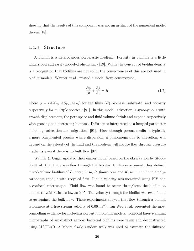
1.4.3 Structure

A biofilm is a heterogenous poroelastic medium. Porosity in biofilms is a little

understood and rarely modeled phenomena [19]. While the concept of biofilm density

is a recognition that biofilms are not solid, the consequences of this are not used in

biofilm models. Wanner et al. created a model from conservation,

∂φ

∂t+∂j

∂z= R (1.7)

where φ = (AXF,i, ASF,i, AεF,i) for the films (F ) biomass, substrate, and porosity

respectively for multiple species i [91]. In this model, advection is synonymous with

growth displacement, the pore space and fluid volume shrink and expand respectively

with growing and decreasing biomass. Diffusion is interpreted as a lumped parameter

including “advection and migration” [91]. Flow through porous media is typically

a more complicated process where dispersion, a phenomena due to advection, will

depend on the velocity of the fluid and the medium will induce flow through pressure

gradients even if there is no bulk flow [92].

Wanner & Guger updated their earlier model based on the observation by Stood-

ley et al. that there was flow through the biofilm. In this experiment, they defined

mixed-culture biofilms of P. aeruginosa, P. fluorescens and K. pneumoniae in a poly-

carbonate conduit with recycled flow. Liquid velocity was measured using PIV and

a confocal microscope. Fluid flow was found to occur throughout the biofilm to

biofilm-to-void ratios as low as 0.05. The velocity through the biofilm was even found

to go against the bulk flow. These experiments showed that flow through a biofilm

is nonzero at a free stream velocity of 0.06 ms−1. van Wey et al. presented the most

compelling evidence for including porosity in biofilm models. Confocal laser-scanning

micrographs of six distinct aerobic bacterial biofilms were taken and deconstructed

using MATLAB. A Monte Carlo random walk was used to estimate the diffusion

26

coefficient, where the walker would stop at each obstacle. Taking the mean squared

difference of the tracer path, the tortuosity, τ of the biofilm was found. While values

for the tortuosity in the direction parallel to the substrate line up well with Maxwell’s

equation

τ =2ε

3− ε(1.8)

values perpendicular to the substrate do not. Values from previous literature all

followed the parallel case. Porosity data was fit with an exponential. These three

values were averaged over depth, so while not height specific, the results captured

the anisotropy. These values were then included in a reaction-diffusion model with a

Monod reaction. The experimental data showed parabolic curves for nutrient trans-

port through biofilms grown on soluble substrates indicating that the biofilm is not as

compact as previously thought. When grown on an insoluble substrate, the nutrient

transport rapidly dropped by the middle of the biofilm. The results agreed well when

compared to literature using stoichiometry for oxygen uptake.

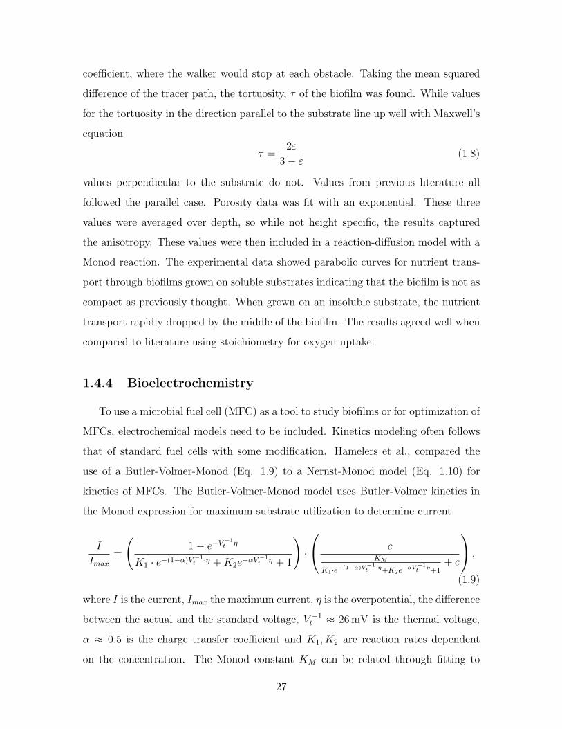
1.4.4 Bioelectrochemistry

To use a microbial fuel cell (MFC) as a tool to study biofilms or for optimization of

MFCs, electrochemical models need to be included. Kinetics modeling often follows

that of standard fuel cells with some modification. Hamelers et al., compared the

use of a Butler-Volmer-Monod (Eq. 1.9) to a Nernst-Monod model (Eq. 1.10) for

kinetics of MFCs. The Butler-Volmer-Monod model uses Butler-Volmer kinetics in

the Monod expression for maximum substrate utilization to determine current

I

Imax=

(1− e−V −1

t η

K1 · e−(1−α)V −1t ·η +K2e−αV

−1t η + 1

)·

cKM

K1·e−(1−α)V−1t ·η+K2e

−αV−1t η+1

+ c

,

(1.9)

where I is the current, Imax the maximum current, η is the overpotential, the difference

between the actual and the standard voltage, V −1t ≈ 26 mV is the thermal voltage,

α ≈ 0.5 is the charge transfer coefficient and K1, K2 are reaction rates dependent

on the concentration. The Monod constant KM can be related through fitting to

27

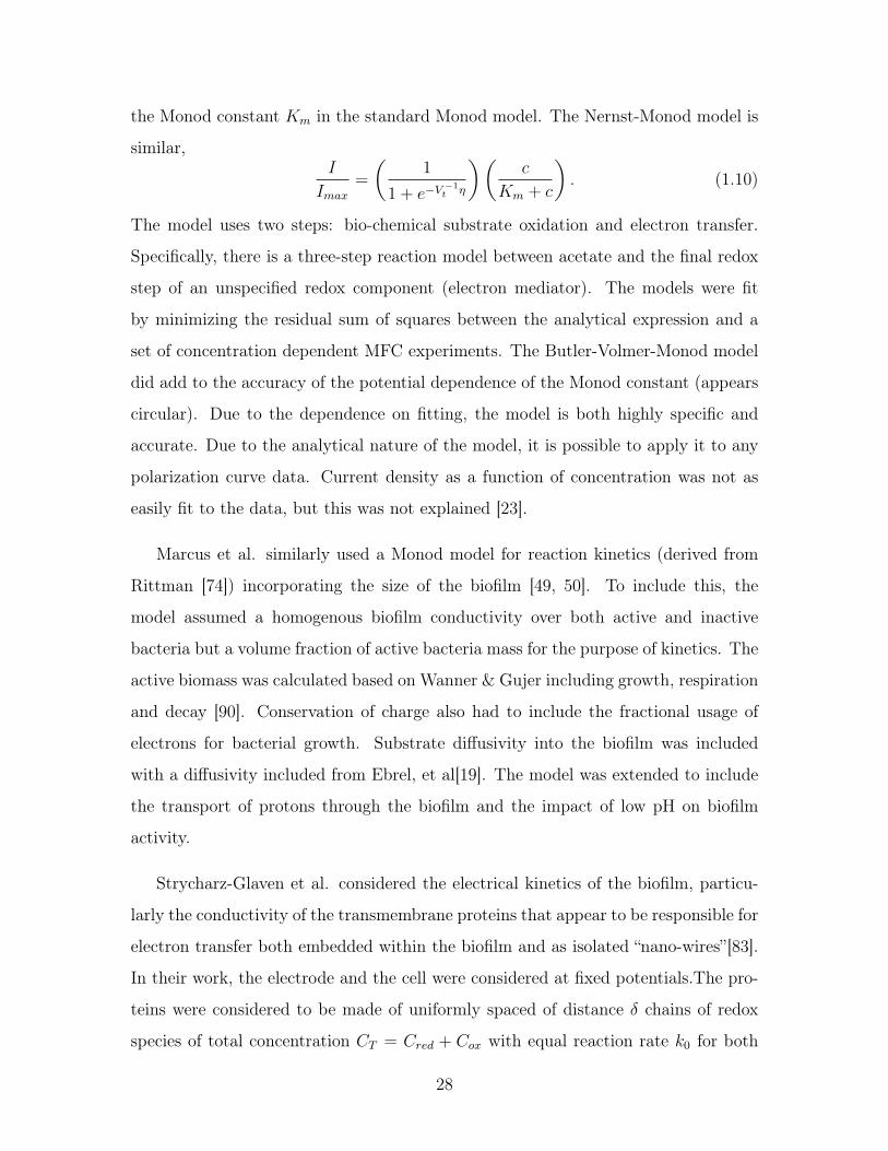
the Monod constant Km in the standard Monod model. The Nernst-Monod model is

similar,I

Imax=

(1

1 + e−V−1t η

)(c

Km + c

). (1.10)

The model uses two steps: bio-chemical substrate oxidation and electron transfer.

Specifically, there is a three-step reaction model between acetate and the final redox

step of an unspecified redox component (electron mediator). The models were fit

by minimizing the residual sum of squares between the analytical expression and a

set of concentration dependent MFC experiments. The Butler-Volmer-Monod model

did add to the accuracy of the potential dependence of the Monod constant (appears

circular). Due to the dependence on fitting, the model is both highly specific and

accurate. Due to the analytical nature of the model, it is possible to apply it to any

polarization curve data. Current density as a function of concentration was not as

easily fit to the data, but this was not explained [23].

Marcus et al. similarly used a Monod model for reaction kinetics (derived from

Rittman [74]) incorporating the size of the biofilm [49, 50]. To include this, the

model assumed a homogenous biofilm conductivity over both active and inactive

bacteria but a volume fraction of active bacteria mass for the purpose of kinetics. The

active biomass was calculated based on Wanner & Gujer including growth, respiration

and decay [90]. Conservation of charge also had to include the fractional usage of

electrons for bacterial growth. Substrate diffusivity into the biofilm was included

with a diffusivity included from Ebrel, et al[19]. The model was extended to include

the transport of protons through the biofilm and the impact of low pH on biofilm

activity.

Strycharz-Glaven et al. considered the electrical kinetics of the biofilm, particu-

larly the conductivity of the transmembrane proteins that appear to be responsible for

electron transfer both embedded within the biofilm and as isolated “nano-wires”[83].

In their work, the electrode and the cell were considered at fixed potentials.The pro-

teins were considered to be made of uniformly spaced of distance δ chains of redox

species of total concentration CT = Cred + Cox with equal reaction rate k0 for both

28

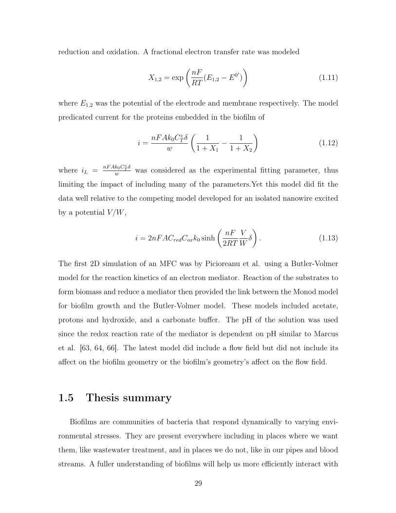
reduction and oxidation. A fractional electron transfer rate was modeled

X1,2 = exp

(nF

RT(E1,2 − E0′)

)(1.11)

where E1,2 was the potential of the electrode and membrane respectively. The model

predicated current for the proteins embedded in the biofilm of

i =nFAk0C

zT δ

w

(1

1 +X1

− 1

1 +X2

)(1.12)

where iL =nFAk0CzT δ

wwas considered as the experimental fitting parameter, thus

limiting the impact of including many of the parameters.Yet this model did fit the

data well relative to the competing model developed for an isolated nanowire excited

by a potential V/W ,

i = 2nFACredCoxk0 sinh

(nF

2RT

V

Wδ

). (1.13)

The first 2D simulation of an MFC was by Picioreanu et al. using a Butler-Volmer

model for the reaction kinetics of an electron mediator. Reaction of the substrates to

form biomass and reduce a mediator then provided the link between the Monod model

for biofilm growth and the Butler-Volmer model. These models included acetate,

protons and hydroxide, and a carbonate buffer. The pH of the solution was used

since the redox reaction rate of the mediator is dependent on pH similar to Marcus

et al. [63, 64, 66]. The latest model did include a flow field but did not include its

affect on the biofilm geometry or the biofilm’s geometry’s affect on the flow field.

1.5 Thesis summary

Biofilms are communities of bacteria that respond dynamically to varying envi-

ronmental stresses. They are present everywhere including in places where we want

them, like wastewater treatment, and in places we do not, like in our pipes and blood

streams. A fuller understanding of biofilms will help us more efficiently interact with

29

them if we are trying to do things like implement them in microbial fuel cells or

remove them from the human body. The tools that to study are beginning to scale

down from “large” reactors to length scale where we can see how they adjust at their

time frame. The models, and our ability to solve those 3D coupled models, are begin-

ning to explain some of the phenomena surrounding the biofilms response to chemical

stresses. We must now begin to look at how they respond to mechanical stresses with

our new tools.

A new tool to study biofilms is developed in the present study. The device is

designed with materials compatible for biofilm growth and compatible with light and

confocal microscopy for direct measurement of the growing biofilm. It is also designed

to incorporate indirect methods of biofilm health like substrate utilization (chemical

oxygen demand measurement), and pH change. As a microbial fuel cell and another

indirect method of monitoring biofilm health, the device is designed to measure total

current and potential of individual electrodes. To interpret these results, a model

is developed that incorporates biofilm growth from a continuous perspective, the

biofilm response to shear stress, and as an addition to existing models, biofilm growth

and response to shear as a poroelastic medium. The device is then tested with one

type of electrode and one flow rate. Preliminary data is presented to guide further

experiments on biofilm substrate compatibility, a biofilms response to shear, and the

optimization of a microbial fuel cell.

30

Chapter 2

Methods for studying biofilms

2.1 Microfluidics

Microfluidics have been used for precision control of liquids and gases in small

devices. Microfluidic devices, like the one presented here, have at least one critical

dimension that is between 10 − 100µm [51]. These devices have a wide range of

geometries and configurations ranging from high-aspect ratios to multiple channels

to embedded electrodes. Modeling the flow through these devices can also range

from simple Navier-Stokes flow with rectangular boundary conditions to much more

complicated models [21].

Most microfluidic devices are governed by laminar flow due to the critical dimen-

sion. Under laminar flow control it has been possible to deposit or etch material on

to or from the surface of channels with a thickness equal to that of the laminar flow

boundary layer. For example, electrically continuous silver wire has been deposited

on glass, gold has been etched from gold, and silicon has been etched from silicon

[78, 32]. These latter processes were accomplished at the diffusion boundary layer

between two parallel reactants flowing under laminar conditions. Using the same

physics, laminar-flow fuel cells (LF-FCs) have been designed to separate the desired

reactions on opposite sides of the separating diffusion boundary layer. These devices

establish laminar-flow between two streams flowing horizontally parallel in shaped

‘Y’-channels, ‘T’-channels, and vertically parallel in ‘L’-channels [36, 35, 30]. These

31

fuel cells have a high volumetric power density and lower internal resistance than fuel

cells where the reactants are separated with a physical barrier.

The advantages to studying microbes and biofilms in a microfluidic device were

explained in Section 1.3. There are also benefits to the direct electrical signal from

microbial fuel cells as an indicator of metabolism (cf. Section 1.2.1). A laminar flow

microbial fuel cell (LF-MFC) combines all the properties above into a unique tool for

studying biofilms.

2.2 Design, Manufacturing, and Materials

2.2.1 Design

This LF-MFC is an x -shaped channel. This design separates the outlet into 3

streams: a consumed anolyte, a consumed catholyte, and a mixed stream. Channel

geometries were tested numerically to maximize electrode surface area and minimize

cross-over without including reaction kinetics (COMSOL Multiphysics, Sweden ).The

3D numerical simulation includes free fluid flow and flow through a porous media to

simulate a non-active biofilm. An active biofilm would consume the concentration the

chances for cross-over would decrease. The porous media was 10µm tall, had a 50%

porosity, a 0.7 m2 permeability and covered the entire anode. These conditions are an

approximation of a biofilm. The resulting channel has a 1.1 mm width over the 20 mm

of fully developed channel length without cross-over. The electrodes are 0.3×20 mm =

6.0× 10−6 m2 spaced 0.5 mm apart. The channel height is 55µm. The inlets and

outlets are angled and the corners rounded to reduce secondary flow. Rounded corners

are also simplify manufacturing and numerical meshing. The velocity is slightly lower

over the porous matrix in simulation, Figure 2-1. The diffusive mixing region is fully

encompassed by the 3rd outlet channel in the simulation Figure 2-2.

Carbon deposited onto glass and onto patterned gold; carbon mixed with poly(dimethyl

siloxane) (PDMS); standard PDMS covered gold electrodes on glass; carbon rods em-

bedded in PDMS; carbon in PDMS and acrylic based devices were either developed

32

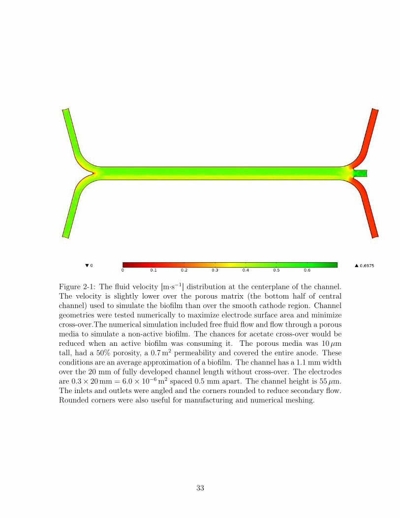
Figure 2-1: The fluid velocity [m·s−1] distribution at the centerplane of the channel.The velocity is slightly lower over the porous matrix (the bottom half of centralchannel) used to simulate the biofilm than over the smooth cathode region. Channelgeometries were tested numerically to maximize electrode surface area and minimizecross-over.The numerical simulation included free fluid flow and flow through a porousmedia to simulate a non-active biofilm. The chances for acetate cross-over would bereduced when an active biofilm was consuming it. The porous media was 10µmtall, had a 50% porosity, a 0.7 m2 permeability and covered the entire anode. Theseconditions are an average approximation of a biofilm. The channel has a 1.1 mm widthover the 20 mm of fully developed channel length without cross-over. The electrodesare 0.3× 20 mm = 6.0× 10−6 m2 spaced 0.5 mm apart. The channel height is 55µm.The inlets and outlets were angled and the corners rounded to reduce secondary flow.Rounded corners were also useful for manufacturing and numerical meshing.

33

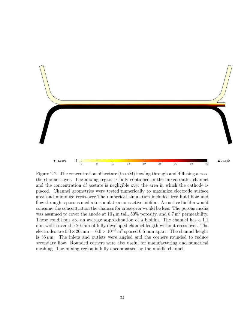
Figure 2-2: The concentration of acetate (in mM) flowing through and diffusing acrossthe channel layer. The mixing region is fully contained in the mixed outlet channeland the concentration of acetate is negligible over the area in which the cathode isplaced. Channel geometries were tested numerically to maximize electrode surfacearea and minimize cross-over.The numerical simulation included free fluid flow andflow through a porous media to simulate a non-active biofilm. An active biofilm wouldconsume the concentration the chances for cross-over would be less. The porous mediawas assumed to cover the anode at 10µm tall, 50% porosity, and 0.7 m2 permeability.These conditions are an average approximation of a biofilm. The channel has a 1.1mm width over the 20 mm of fully developed channel length without cross-over. Theelectrodes are 0.3×20 mm = 6.0× 10−6 m2 spaced 0.5 mm apart. The channel heightis 55µm. The inlets and outlets were angled and the corners rounded to reducesecondary flow. Rounded corners were also useful for manufacturing and numericalmeshing. The mixing region is fully encompassed by the middle channel.

34

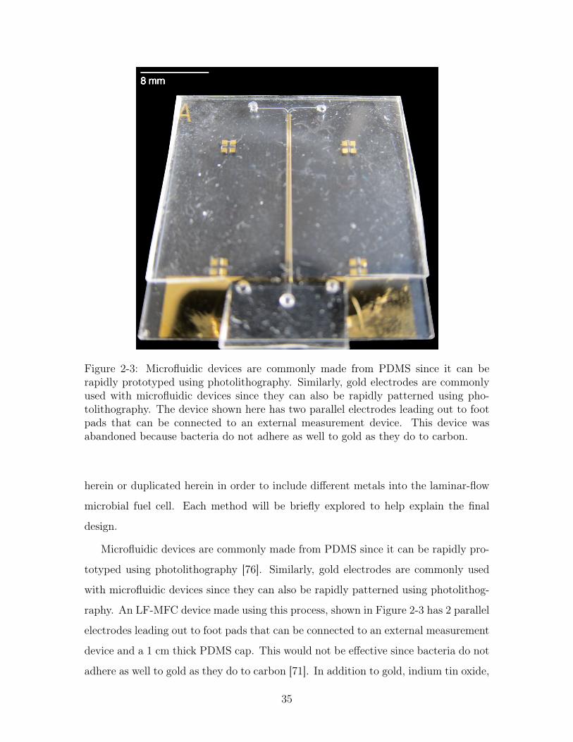
Figure 2-3: Microfluidic devices are commonly made from PDMS since it can berapidly prototyped using photolithography. Similarly, gold electrodes are commonlyused with microfluidic devices since they can also be rapidly patterned using pho-tolithography. The device shown here has two parallel electrodes leading out to footpads that can be connected to an external measurement device. This device wasabandoned because bacteria do not adhere as well to gold as they do to carbon.

herein or duplicated herein in order to include different metals into the laminar-flow

microbial fuel cell. Each method will be briefly explored to help explain the final

design.

Microfluidic devices are commonly made from PDMS since it can be rapidly pro-

totyped using photolithography [76]. Similarly, gold electrodes are commonly used

with microfluidic devices since they can also be rapidly patterned using photolithog-

raphy. An LF-MFC device made using this process, shown in Figure 2-3 has 2 parallel

electrodes leading out to foot pads that can be connected to an external measurement

device and a 1 cm thick PDMS cap. This would not be effective since bacteria do not

adhere as well to gold as they do to carbon [71]. In addition to gold, indium tin oxide,

35

aluminum, chromium, an silicon can all be micro-patterned using photolithography

which may be a viable option if bacteria can be acclimated to those substrates.

Standard lithographic techniques can be used to produce carbon electrodes. Yet

this method is time consuming. Sputter coated graphite can be produced using two

graphite targets in an 80% Argon 20% Nitrogen environment with a DC and RF

power source at 250 W for 52 minutes in an AJA international Orion 5 to produce a

200 nm thick layer. The amorphous carbon produced is not conductive. A novel way

around this is to deposit a conductive layer first under the graphite layer as done in

Figure 2-4. Gold was initially deposited onto patterned photoresist using electron-

beam deposition and then developed. Carbon is then deposited onto the entire wafer.

This is then patterned again. The non-patterned graphite is removed using oxygen

plasma. The resulting carbon deposited will not be the same as graphite or most

common forms of carbon and the presence of the underlying conductive layer will

definitely impact any the electrochemical/catalytic activity of the assembly. Yet, the

resulting assembly is conductive and usable in a PDMS-based device. There are other

means of making gold a biocompatible electrode including the use of self-assembled

monolayers of thiols and carbon nanotubes but these avenues are not practical for

scale-up.

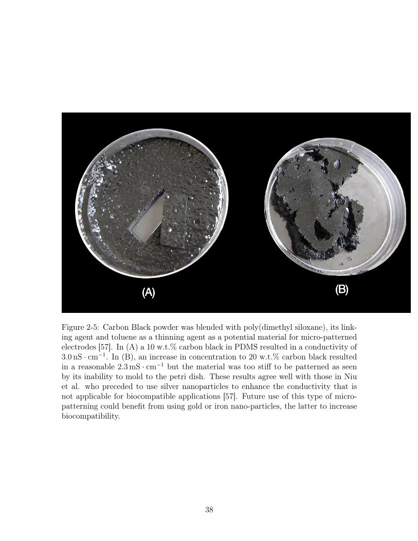
Carbon Black powder was blended with poly(dimethyl siloxane), its linking agent

and toluene, a thinning agent, as a material for micro-patterned electrodes [57], Figure

2-5. In Figure 2-5 (A) a 10 w.t.% carbon black in PDMS resulted in a conductivity

of 2.97 nS · cm−1. In Figure 2-5(B), an increase in concentration to 20 w.t.% carbon

black resulted in a reasonable conductivity 2.3 mS · cm−1 but the material was too

stiff to be patterned into anything useful as seen by its inability to mold to the

petri dish. These results agree well with those in Niu et al. who preceded to use

silver nanoparticles to enhance the conductivity. This method could not be done for

biocompatible applications. Future use of this type of micro-patterning could benefit

from using gold or iron nano-particles, the latter to increase biocompatibility. The

design in Figure 2-6 is limited in electrode material. This can be overcome by placing

a physical barrier between two pockets, Figure 2-7. Two pockets 4 x 20 mm, large

36

8 mm

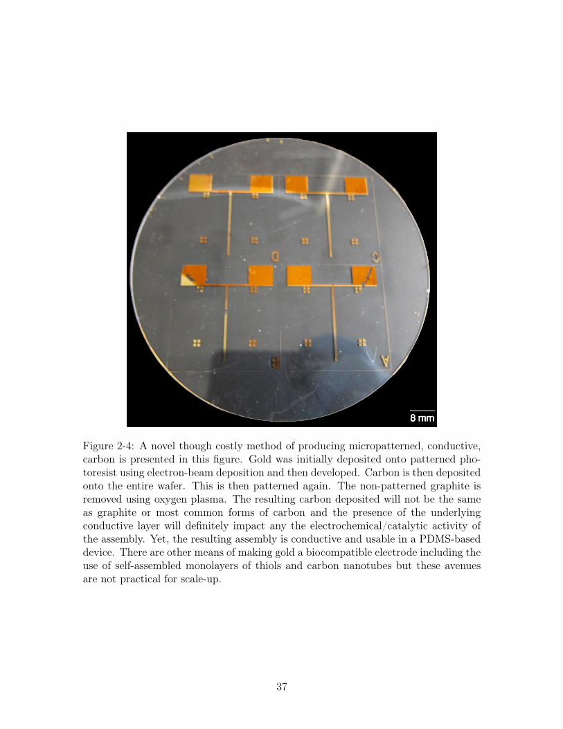
Figure 2-4: A novel though costly method of producing micropatterned, conductive,carbon is presented in this figure. Gold was initially deposited onto patterned pho-toresist using electron-beam deposition and then developed. Carbon is then depositedonto the entire wafer. This is then patterned again. The non-patterned graphite isremoved using oxygen plasma. The resulting carbon deposited will not be the sameas graphite or most common forms of carbon and the presence of the underlyingconductive layer will definitely impact any the electrochemical/catalytic activity ofthe assembly. Yet, the resulting assembly is conductive and usable in a PDMS-baseddevice. There are other means of making gold a biocompatible electrode including theuse of self-assembled monolayers of thiols and carbon nanotubes but these avenuesare not practical for scale-up.

37

(A) (B)

Figure 2-5: Carbon Black powder was blended with poly(dimethyl siloxane), its link-ing agent and toluene as a thinning agent as a potential material for micro-patternedelectrodes [57]. In (A) a 10 w.t.% carbon black in PDMS resulted in a conductivity of3.0 nS · cm−1. In (B), an increase in concentration to 20 w.t.% carbon black resultedin a reasonable 2.3 mS · cm−1 but the material was too stiff to be patterned as seenby its inability to mold to the petri dish. These results agree well with those in Niuet al. who preceded to use silver nanoparticles to enhance the conductivity that isnot applicable for biocompatible applications [57]. Future use of this type of micro-patterning could benefit from using gold or iron nano-particles, the latter to increasebiocompatibility.

38

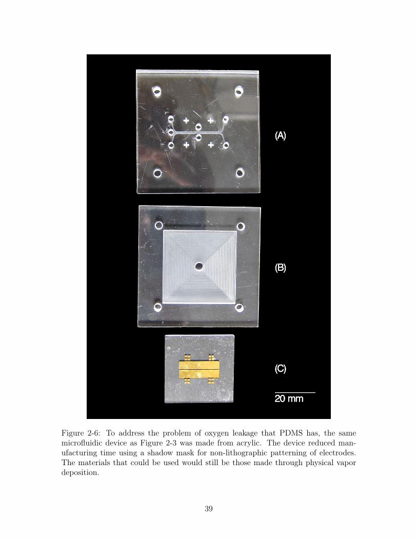
(A)

(B)

(C)

20 mm

Figure 2-6: To address the problem of oxygen leakage that PDMS has, the samemicrofluidic device as Figure 2-3 was made from acrylic. The device reduced man-ufacturing time using a shadow mask for non-lithographic patterning of electrodes.The materials that could be used would still be those made through physical vapordeposition.

39

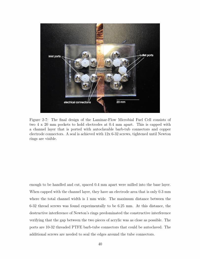
inlet ports outlet ports

electrical connections 20 mm

Figure 2-7: The final design of the Laminar-Flow Microbial Fuel Cell consists oftwo 4 x 20 mm pockets to hold electrodes at 0.4 mm apart. This is capped witha channel layer that is ported with autoclavable barb-tub connectors and copperelectrode connectors. A seal is achieved with 12x 6-32 screws, tightened until Newtonrings are visible.

enough to be handled and cut, spaced 0.4 mm apart were milled into the base layer.

When capped with the channel layer, they have an electrode area that is only 0.3 mm

where the total channel width is 1 mm wide. The maximum distance between the

6-32 thread screws was found experimentally to be 6.25 mm. At this distance, the

destructive interference of Newton’s rings predominated the constructive interference

verifying that the gap between the two pieces of acrylic was as close as possible. The

ports are 10-32 threaded PTFE barb-tube connectors that could be autoclaved. The

additional screws are needed to seal the edges around the tube connectors.

40

2.2.2 Manufacturing

The LF-MFC is designed as a tool to study in situ electroactive biofilm formation.

The LF-MFC is cut from cast acrylic, poly(methyl methacrylate) (PMMA). PMMA

has a refractive index of n25D = 1.49[3]. PDMS has a refractive index of 1.403. While

the refractive index of PDMS is closer to that of water, the working fluid, PMMA

is closer to that of glass used in microscopes so there is a trade off either way. The

water absorption of both PDMS and cast PMMA is between 0.2 - 0.8% so there is no

difference. The gas diffusion rate of oxygen through acrylic is 3.3−33× 10−9 cm2 · s−1

[27]. The gas diffusion rate of oxygen through PDMS is 3.4− 16× 10−5 cm2 · s−1[8].

The high oxygen diffusion rate in PDMS is typically used to help grow aerobic bacteria

and human tissue. This 4 orders of magnitude difference between acrylic and PDMS

can mean the difference between life and death for strict anaerobic bacteria [77, 40].

PDMS was used as the channel material for the other two LF-MFCs that exist which

may explain their low current generation [45, 46]. 1

The top and bottom half of the LF-MFC are cut from cast acrylic using a laser

cutter (Epilog Laser , USA). This allows for rapid cutting of the screw holes but not

the channels since the machine’s precision is ±2 mm. The channel and pockets are

cut on a Microlution 363-S (Microlution, Chicago, IL, USA). The mill has a reported

accuracy of ±2µm but, as will be shown, can be pushed into the 100 nm range. The

tool parameters and setups are optimized to yield a smooth surface finish and preserve

flow geometry. Any machining of a microfluidic device with similar features should

use similar parameters. This mill is equipped with a 56,000 rpm, air-turbine spindle

with a 3.175 mm (1/8”) dia chuck, flood coolant and air coolant. The pallet working

area is 60× 58 mm(x× y) and a custom fixture was made to hold each part in place

to preserve alignment. The rotational velocity is limited to 48,000 rpm to minimize

wear on the spindle bearings. The channels are cut using a 0.254 mm (0.01in) 4 flute

end mill. This was chosen over smaller end mills and 2 flute end mills to minimize

1To address the problem of oxygen leakage that PDMS has, the same microfluidic device asFigure 2-3 was made from acrylic. Manufacturing time was reduced by using a shadow mask fornon-lithographic patterning of electrodes. The materials that could be used would still be thosemade through physical vapor deposition.

41

scalloping, the formation of ridges between cuts of a mill. The chip load, the size of

chips cut by the each flute, is 1.9µm/tooth which gave a feed rate of 365 mm/min.

Optimization of the cutting parameters matched the formula found by Vogler et al.,

Ra ∝CL2

0.5D, (2.1)

where Ra is the surface roughness, CL is the chip-load [µm/tooth], and D is the

tool diameter [µm] [89]. A proportionality constant of 5 for acrylic was calculated by

cutting with a 0.508, 0.381 and 0.254 mm (0.02, 0.015 and 0.01 in) diameter tools.

All mill paths and G-code are generated using MasterCam X5 (CNC Software,

Inc, Tolland, CT, USA). The tool path for the channels is a “2D pocket Dynamic Area

Mill.” This produces an optimal path for cornering. A stepover of 5% diameter is

used to minimize scalloping. Scalloping can be reduced by using a finish pass. Since

the depth of cut for this part is 55µm, any finish pass would produce nanometer

sized chips that could not be properly cleared with flood coolant. Atomized coolant

is recommended for clearing the small chips in micro-machining to improve surface

finish, minimize tool wear and reduce part temperature. High temperature can cause

the welding of chips to the part [31]. The mill used here is not equipped with atomized

coolant but the measured surface finish is ∼ 100 nm and there is no indication of

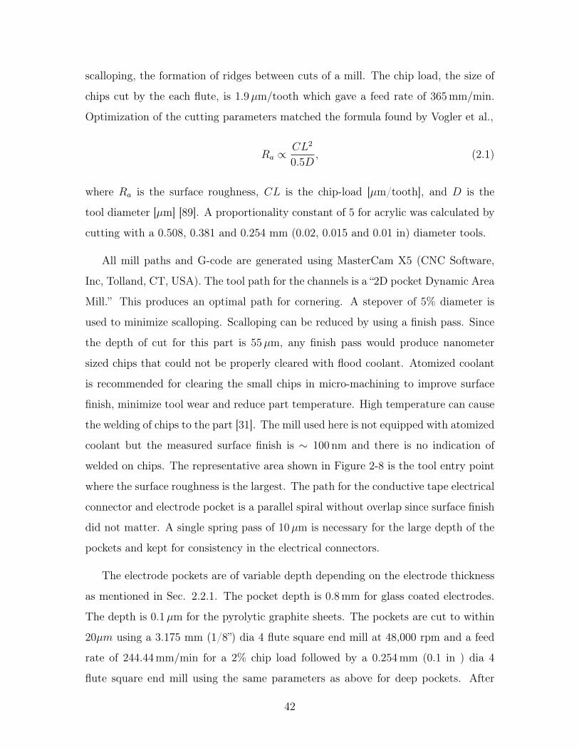
welded on chips. The representative area shown in Figure 2-8 is the tool entry point

where the surface roughness is the largest. The path for the conductive tape electrical

connector and electrode pocket is a parallel spiral without overlap since surface finish

did not matter. A single spring pass of 10µm is necessary for the large depth of the

pockets and kept for consistency in the electrical connectors.

The electrode pockets are of variable depth depending on the electrode thickness

as mentioned in Sec. 2.2.1. The pocket depth is 0.8 mm for glass coated electrodes.

The depth is 0.1µm for the pyrolytic graphite sheets. The pockets are cut to within

20µm using a 3.175 mm (1/8”) dia 4 flute square end mill at 48,000 rpm and a feed

rate of 244.44 mm/min for a 2% chip load followed by a 0.254 mm (0.1 in ) dia 4

flute square end mill using the same parameters as above for deep pockets. After

42

0 µm!

2.93009!

!" #"

Figure 2-8: The representative area shown in Figure 2-8 is the tool entry point wherethe surface roughness is the largest. A gradient heat map of the height of the milledsurface is shown in (B). The optical image of the same surface is shown in (A). Theaverage surface roughness was calculated from this as ∼ 100 nm.

machining the device, the parts are cleaned in a sonicator in Citranox R© to remove

coolant oil and any chips leftover from the cutting processes. Ultrasonic cleaning is

recommended to remove small (< 2µm) chips that could get stuck in the corners of

the channels. Citranox R© is a organic acid cleaner and any remaining citric acid must

be removed by thorough rinsing (sonication) with deionized water. A final polishing

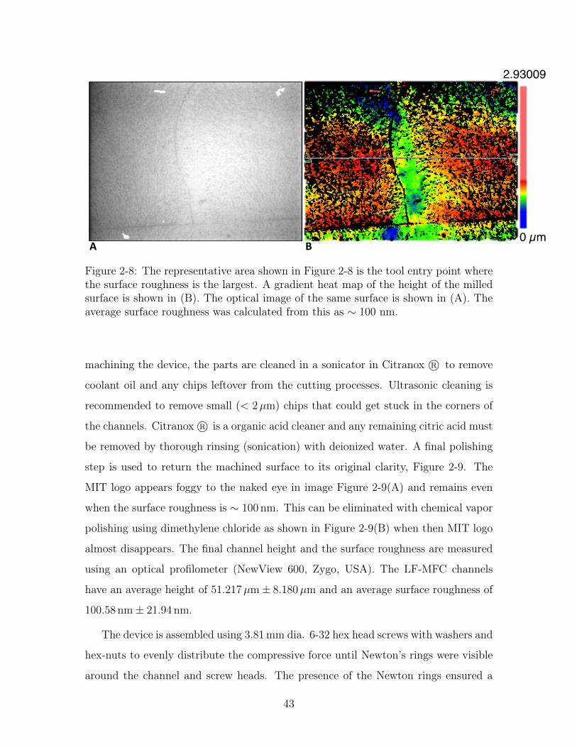
step is used to return the machined surface to its original clarity, Figure 2-9. The

MIT logo appears foggy to the naked eye in image Figure 2-9(A) and remains even

when the surface roughness is ∼ 100 nm. This can be eliminated with chemical vapor

polishing using dimethylene chloride as shown in Figure 2-9(B) when then MIT logo

almost disappears. The final channel height and the surface roughness are measured

using an optical profilometer (NewView 600, Zygo, USA). The LF-MFC channels

have an average height of 51.217µm± 8.180µm and an average surface roughness of

100.58 nm± 21.94 nm.

The device is assembled using 3.81 mm dia. 6-32 hex head screws with washers and

hex-nuts to evenly distribute the compressive force until Newton’s rings were visible

around the channel and screw heads. The presence of the Newton rings ensured a

43

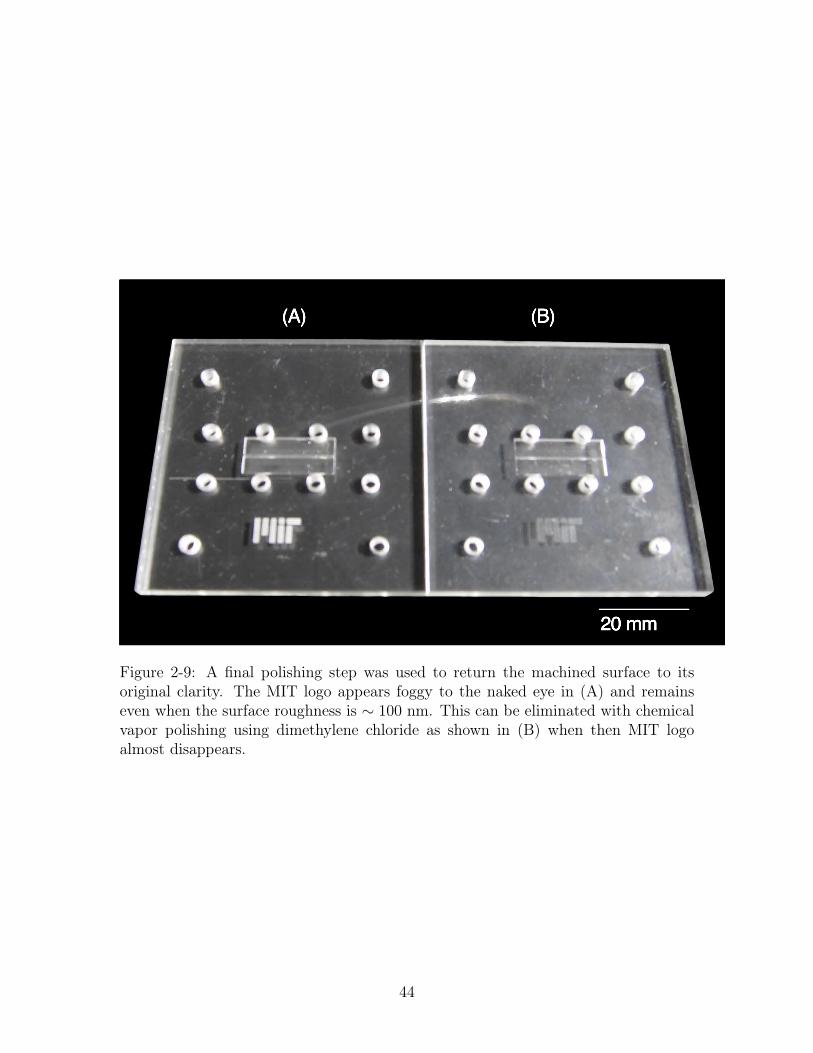
Figure 2-9: A final polishing step was used to return the machined surface to itsoriginal clarity. The MIT logo appears foggy to the naked eye in (A) and remainseven when the surface roughness is ∼ 100 nm. This can be eliminated with chemicalvapor polishing using dimethylene chloride as shown in (B) when then MIT logoalmost disappears.

44

seal. The channel inlets and outlets were 10-32 thread hose-barb tube connectors.

2.2.3 Materials

When bacteria colonize a surface they can cause a variety of problems and, in

certain cases, some benefit. When bacteria colonize submerged or buried pipes with

water or other substances through it, they can cause corrosion on the outside or

inside[20]. In pipes, on ship’s hulls and propellors biofilms can cause substantial

drag losses. When bacteria colonize doorknobs, bench-tops and medical equipment

they can increase the spread of disease. On the other hand, when bacteria colonize

membranes in membrane biological reactors for wastewater treatment they decrease

the footprint of water treatment plants.

The choice of substrate is critical to the cells growth and survival in an engineered

environment[7]. When bacteria colonize insoluble electron acceptors, power can be

harvested from them. The surface area of the substrate controls the upper limit of a

monolayer of bacteria that can be in one device. The surface roughness, wettability,

and electrostatic interactions determine whether or not the bacteria will bond to the

surface [9]. The catalytic activity will determine the reversibility and viability of

this interaction. Finally, the conductivity will determine how much current will be

generated by the device. In order to quantify this interaction, multiple materials were

tested in the same device.

All electrodes are cleaned in an ultrasonic bath in Citranox R©, acetone then iso-

proponal for 5 minutes each. They are imaged using scanning electron microscopy

(VEGA3 SEM, Tescan, CZE). Surface roughness is measured using optical profilome-

try. Atomic force microscopy in tapping mode (Nanoscope IV Dimension 3100 SPM,

Veeco, USA ) is used to measure the surface roughness for surfaces where the surface

features were smoother than the resolution of the optical profilometer. Scanning elec-

tron microscope images of each surface are provided in Figures 2-10-2-11. Surface free

energy is calculated using contact angle measurements on each substrate. Deionized

water and ethylene glycol were used as the polar substances while 1-bromonapthalene

is used as the polar substance. Variation in surface energy measurements is common.

45

!" !# $%&&

'( $%&&

$%&&

)*

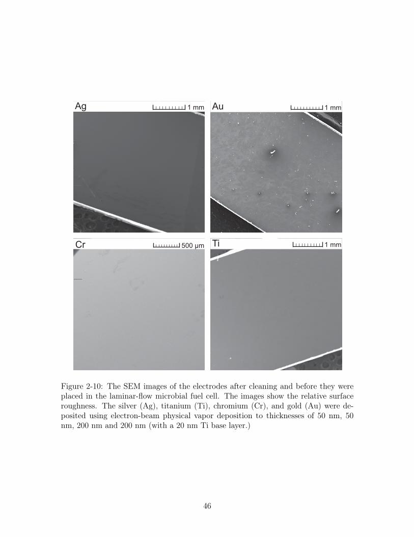
Figure 2-10: The SEM images of the electrodes after cleaning and before they wereplaced in the laminar-flow microbial fuel cell. The images show the relative surfaceroughness. The silver (Ag), titanium (Ti), chromium (Cr), and gold (Au) were de-posited using electron-beam physical vapor deposition to thicknesses of 50 nm, 50nm, 200 nm and 200 nm (with a 20 nm Ti base layer.)

46

!"##$%& '()* !"##

+,- ./ !"##

'0

!"##

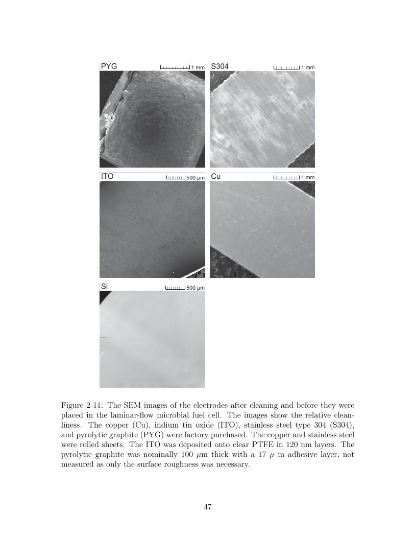
Figure 2-11: The SEM images of the electrodes after cleaning and before they wereplaced in the laminar-flow microbial fuel cell. The images show the relative clean-liness. The copper (Cu), indium tin oxide (ITO), stainless steel type 304 (S304),and pyrolytic graphite (PYG) were factory purchased. The copper and stainless steelwere rolled sheets. The ITO was deposited onto clear PTFE in 120 nm layers. Thepyrolytic graphite was nominally 100 µm thick with a 17 µ m adhesive layer, notmeasured as only the surface roughness was necessary.

47

Variations can be due to the anisotropy of the crystal surface of copper or zinc and

the deposited nano-clusters of titanium, chromium, silver, or gold. This theory will

not be corrected here and the results are used as is.

Interactions of the bacteria and the surface can be modeled using DLVO theory

[16, 12, 28]. The surface energies of solids cannot be tabulated in the same way surface

energies of liquids can be tabulated at specific temperatures due to interactions of

the liquid with the crystal structure [17]. The liquid used to determine the surface

energy, surface roughness, the orientation of lattice planes, and temperature can all

impact the measurements. With the current models, surface energy calculations are

useful for trends between materials, not rigid design parameters. Regardless of which

model is used, the Gibbs Free energy of interaction, ∆GTOT1234 , is the sum of all the

Gibbs energy, ∆G1234, in the system

∆GTOT1234 =

∑∆G1234 (2.2)

where 1 is the solid, 2, the liquid, 3, the particle, and 4, the vapor. In the present

model,

∆GTOTlsb = ∆GLW

lsb + ∆GABlsb + ∆GEL

lsb (2.3)

where l is the liquid medium, s is the solid substrate, b is the bacteria. The models

are LW for Lipshitz- van der Waals interaction, AB for Lewis acid-base interaction

and EL for electrostatic interaction. The Gibbs free energy between the liquid and

the surface is

∆Gls = ∆GLWls + ∆GAB

ls = 2

(√γLWs γLWl +

√γ+s γ−l +

√γ−s γ

+l

), (2.4)

where γ is the surface free energy. This is related to the contact angle between the

surface and liquid, θ through Young’s equation

(1 + cos θ)γl = 2

(√γLWs γLWl +

√γ+s γ−l +

√γ−s γ

+l

). (2.5)

48

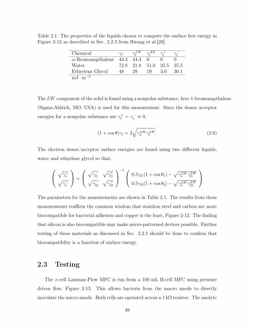
Table 2.1: The properties of the liquids chosen to compute the surface free energy inFigure 2-12 as described in Sec. 2.2.3 from Hwang et al.[28].

Chemical γl γLWl γABl γ+l γ−l

α-Bromonapthalene 44.4 44.4 0 0 0Water 72.8 21.8 51.0 25.5 25.5Ethyelene Glycol 48 29 19 3.0 30.1mJ ·m−2

The LW component of the solid is found using a nonpolar substance, here 1-bromonapthalene

(Sigma-Aldrich, MO, USA) is used for this measurement. Since the donor/acceptor

energies for a nonpolar substance are γ+l = γ−s ≈ 0,

(1 + cos θ)γl = 2√γLWs γLWl . (2.6)

The electron donor/acceptor surface energies are found using two different liquids,

water and ethyelene glycol so that,

√γ+s√γ−s

=

√γ−l1

√γ+l1√

γ−l2√γ+l2

−1 0.5γl1(1 + cos θ1)−√γLWs γLWl1

0.5γl2(1 + cos θ2)−√γLWs γLWl2

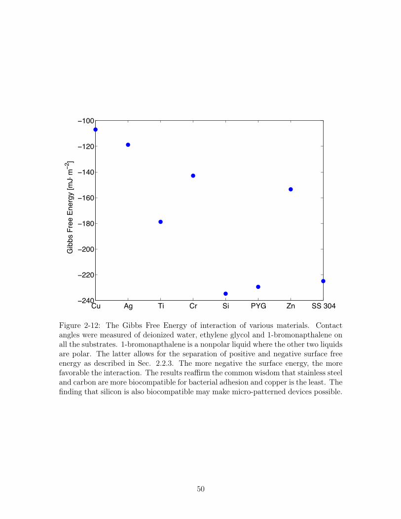
The parameters for the measurements are shown in Table 2.1. The results from these

measurements reaffirm the common wisdom that stainless steel and carbon are more

biocompatible for bacterial adhesion and copper is the least, Figure 2-12. The finding

that silicon is also biocompatible may make micro-patterned devices possible. Further

testing of these materials as discussed in Sec. 2.2.1 should be done to confirm that

biocompatiblity is a function of surface energy.

2.3 Testing

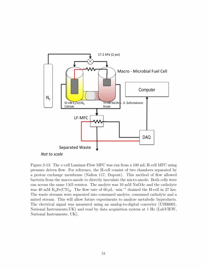
The x -cell Laminar-Flow MFC is run from a 100 mL H-cell MFC using pressure

driven flow, Figure 2-13. This allows bacteria from the macro anode to directly

inoculate the micro-anode. Both cells are operated across a 1 kΩ resistor. The anolyte

49

Cu Ag Ti Cr Si PYG Zn SS 304−240

−220

−200

−180

−160

−140

−120

−100

Gib

bs F

ree

Ener

gy [m

J⋅ m−2

]

Figure 2-12: The Gibbs Free Energy of interaction of various materials. Contactangles were measured of deionized water, ethylene glycol and 1-bromonapthalene onall the substrates. 1-bromonapthalene is a nonpolar liquid where the other two liquidsare polar. The latter allows for the separation of positive and negative surface freeenergy as described in Sec. 2.2.3. The more negative the surface energy, the morefavorable the interaction. The results reaffirm the common wisdom that stainless steeland carbon are more biocompatible for bacterial adhesion and copper is the least. Thefinding that silicon is also biocompatible may make micro-patterned devices possible.

50

N2!10 mM NaOAc + G. Sulfurreducens Anode!

50 mM K3Fe(CN)6!Cathode!

DAQ!

Computer!

17.2%kPa%(2%psi)%

Separated%Waste%Not$to$scale$

LF6MFC%

Macro%6%Microbial%Fuel%Cell%

Figure 2-13: The x -cell Laminar-Flow MFC was run from a 100 mL H-cell MFC usingpressure driven flow. For reference, the H-cell consist of two chambers separated bya proton exchange membrane (Nafion 117, Dupont). This method of flow allowedbacteria from the macro-anode to directly inoculate the micro-anode. Both cells wererun across the same 1 kΩ resistor. The anolyte was 10 mM NaOAc and the catholytewas 40 mM K3Fe(CN)6. The flow rate of 60µL ·min−1 drained the H-cell in 27 hrs.The waste streams were separated into consumed anolyte, consumed catholyte and amixed stream. This will allow future experiments to analyze metabolic byproducts.The electrical signal was measured using an analog-to-digital converter (USB6001,National Instruments,UK) and read by data acquisition system at 1 Hz (LabVIEW,National Instruments, UK).

51

0.04 0.045 0.05 0.055 0.06−1.5

−1

−0.5

0

0.5

1

1.5

2

2.5 x 10−6

Voltage (V) vs Counte r Elec trode ( [F e(CN ) 6]3! | [F e(CN ) 6]

4!)

Curr

ent(A

)

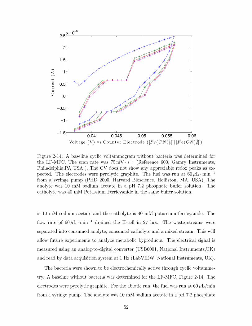
Figure 2-14: A baseline cyclic voltammogram without bacteria was determined forthe LF-MFC. The scan rate was 75 mV · s−1 (Reference 600, Gamry Instruments,Philadelphia,PA USA ). The CV does not show any appreciable redox peaks as ex-pected. The electrodes were pyrolytic graphite. The fuel was run at 60µL ·min−1

from a syringe pump (PHD 2000, Harvard Bioscience, Holliston, MA, USA). Theanolyte was 10 mM sodium acetate in a pH 7.2 phosphate buffer solution. Thecatholyte was 40 mM Potassium Ferricyanide in the same buffer solution.

is 10 mM sodium acetate and the catholyte is 40 mM potassium ferricyanide. The

flow rate of 60µL ·min−1 drained the H-cell in 27 hrs. The waste streams were

separated into consumed anolyte, consumed catholyte and a mixed stream. This will

allow future experiments to analyze metabolic byproducts. The electrical signal is

measured using an analog-to-digital converter (USB6001, National Instruments,UK)

and read by data acquisition system at 1 Hz (LabVIEW, National Instruments, UK).

The bacteria were shown to be electrochemically active through cyclic voltamme-

try. A baseline without bacteria was determined for the LF-MFC, Figure 2-14. The

electrodes were pyrolytic graphite. For the abiotic run, the fuel was run at 60µL/min

from a syringe pump. The anolyte was 10 mM sodium acetate in a pH 7.2 phosphate

52

buffer solution. The catholyte was 40 mM Potassium Ferricyanide in the same buffer

solution. The scan rate is 75 mV/s. The abiotic CV did not show any apprecia-

ble redox peaks so the cell was operating without any leaks of copper, oxygen, or

cross-over.

2.4 Modeling biofilm dynamics

Current models of biofilm dynamics have divided biofilm activity into four pro-

cesses: growth, detachment, structure and bioelectrochemistry (cf. Sec. 1.4). In

this model, the fluid flow is assumed to control the growth, detachment and struc-

ture of the biofilm so such a division is not possible. The mass and fluid transport

in a biofilm can be broken into transport through (1) the bulk system outside of

the boundary layer, a distance δ = max(δm, δl) away from the biofilm, (2) the mass

and fluid boundary layer region of thickness δm, δl respectively, (3) the interface be-

tween the bulk and the biofilm, 4) the biofilm and 5) the biofilm electrode interface

(cf. Figure 1-1). Furthermore, any biofilm process is a catalytic process subject to

Michaeliis-Menten (Monod) kinetics, growth, death, and loss [68, 19]. In what follows

the unsteady Stokes equation is used to establish the hydrodynamic boundary layer

(1) and (2) from above. An advection-diffusion-reaction equation is then solved for

solute to calculate the concentrations field of the mass transfer boundary layer. The

porosity of the biofilm will determine the flow through the biofilm and is included

as a source term. The relation between shear stress and biofilm loss has been ex-

perimentally determined, but existing models have come short of using structural

properties of a biofilm to predict biofilm loss as a function of shear stress [74, 34].

Here, shear between the bulk flow and the biofilm defines the interface and also cell

loss and growth by assuming the biofilm is a poroelastic medium. As mentioned in

Sec. 1.3, a microbial fuel cell produces a direct electrical signal that is a function of:

biofilm health, metabolism, and size. A description of a Butler-Volmer kinetic equa-

tion, interaction 5 in the above, is given here, not including mechanisms for electron

conduction or capacitance, but not solved for.

53

2.4.1 Fluid Flow

The fluid subsystem can be modeled using the Navier-Stokes equation,

(∂u

∂t+ u · ∇u

)= ν∇2u− 1

ρ∇p− ν

ku, (2.7)

for velocity vector u, pressure p, ensemble (or solvent water) kinematic viscosity ν

(or ν0), and ensemble (or solvent water) density ρ (or ρ0). The additional term on

the right hand side is the Darcy pressure term used to find the velocity in the porous

media with permeability k. Since the permeability is different in the z, y directions,

this term is more active in one dimension than the other. This equation is coupled

with the continuity equation for an incompressible fluid,

∇ · u = 0 (2.8)

Equations 2.7 and 2.8 can be simplified by looking at the 2D problem, in dimensions

〈y, z〉 as shown in Figure 1-1. The equations can be further simplified through scaling

analysis. Let the velocity scale in the direction of flow as uy = V uy and uz = Wuz

where V is the inlet velocity and the scaling of W will be determined later. D is the

length of the biofilm so that the length scale along the direction of flow is y = Dy

and z = Lcz in the direction perpendicular to flow where Lc is a characteristic length.

The characteristic length in the biofilm is the biofilm thickness, Lc = Lf . Biofilms

tend to not form outside the viscous boundary layer of the fluid, so the characteristic

length scale in the fluid is the boundary layer thickness Lc = δl along the biofilm (for

biofilm streamers) or along the surface it is growing on. The characteristic time for

the fluid is τl = DV. The latter scaling will be balanced with scaling of the biofilm

growth and substrate transport later. Substituting these relations into Eq. 2.7 yields,

(V

τl

∂uy

∂t+V 2

Duy∂uy∂y

+VW

Lcuz∂uy∂z

)= ν

V

D2

∂2uy∂y2

+ νV

L2c

∂2uy∂z2(

W

τ

∂uz

∂t+VW

Duy∂uz∂y

+W 2

Lcuz∂uz∂z

)= ν

W

D2

∂2uz∂y2

+ νW

L2c

∂2uz∂z2

.

54

Also substituting the scaling into the continuity equation, Eq.2.8 yields,

V

D

∂uy∂y

+W

Lc

∂uz∂z

= 0, (2.9)

then the vertical velocity scales as W ∼ V LcD

. This results in two separate scalings,

ReLc =V Lcν0

and a =LcD,

the Reynolds number and an aspect ratio respectively. The upper bounds of the length

of the biofilm vary experimentally from ∼ 1 mm, for partially detached streamers in

microfluidic channels, to 10 cm in pipes, again within the boundary layer where the

flow goes to 1× 10−3 m · s−1. The maximum biofilm thickness is about 60µm. The

maximum biofilm thickness is flow and orientation dependent which should be studied

in the future. Assuming that the viscosity and the density of the ensemble are that

of the water, ReLc < 0.01 and the flow will always be laminar. Therefore the flow

falls in the Stokes flow regime. The time dependent term remains to establish the

boundary layer. Thus Eq. 2.7 becomes

∂u

∂t= ν∇2u− 1

ρ∇p− ν

ku. (2.10)

The pressure is scaled by letting p = ρV 2p and the permeability by letting k = LcDk.

James et al. and Tachie et al. did show the Brinkman model predicts a slip velocity

that is 70% higher than the actual slip velocity but researches still find the Brinkman

model computationally simpler and useful [29, 84, 55]. The experimentally determined

permeability scales with porosity

k ' φ3

(1− φ)2(2.11)

55

where φ is the porosity [52]. This scaling is taken to be equal for the first approxi-

mation. Substituting the scalings back in to Eq. 2.10 gives a dimensionless equation

∂uy

∂t=

Re−1Lc

a

(a2∂

2uy∂y2

+∂2uy∂z2

)− ∂p

∂y−Re−1

Lc

(1− φ)2

φ3uy (2.12)

∂uz

∂t=

Re−1Lc

a

(a2∂

2uz∂y2

+∂2uz∂z2

)− 1

a2

∂p

∂z−Re−1

Lc

(1− φ)2

φ3uy (2.13)

where the term on the left is the change in velocity over time, the first term on the

right is the diffusion of momentum, the second term is the flow due to a pressure

gradient and the last term is drag due to the porosity.

2.4.2 Solute Advection - Diffusion - Reaction

Since biofilms consume substrates, produce new chemicals from substrates, and

produce waste products including ions, everything that obeys the following equations

is a solute. A solute with concentration c will change with respect to time by flux

into and out of the system and any creation or consumption of the substrate,

∂(cφ)

∂t+∇ ·N = R, (2.14)

where φ is the porosity of the medium, N is the total flux, and R is the reaction rate.

Multiple solutes may be coupled together through the reaction term or the flux term

(binary diffusion). It is assumed that the viscosity and density of the fluid do not

depend on concentration ρ 6= ρ(c) and µ 6= µ(c) which makes the flux terms almost

linear.

The advective flux is the rate at which the solute is carried by the fluid and is

given by

Nadv = uc, (2.15)

where u is the velocity of the bulk. The diffusive flux is the flux of the solute caused

56

by concentration gradients across the medium.The diffusive flux follows Fick’s law,

Ndiff = −Dd∇c, (2.16)

where the Fickian diffusivity, Dd is related to the molecular diffusivity D0. by the

porosity and the tortuosity tensor T from [88]

Dd =φ

TyTzD0

Tz 0

0 Ty

. (2.17)

The dispersive flux is similarly

Ndisp = −Dm∇c. (2.18)

where mechanical diffusion (dispersion), Dm, typically dominates the diffusivity. In

porous media, longitudinal dispersion dominates transverse dispersion and the diffu-

sion coefficient is a tensor:

Dm = αT |u|δij + (αL − αT )uiuj|u|

= αT |u|1 + (αL − αT )

u2x

|u|uxuy|u|

uxuy|u|

u2y

|u|

where αL,T is the longitudinal and transverse dispersivity respectively (αT ∼ 0.1αL).

In a microbial fuel cell, the flux of charged particles responds to the electric field

between the electrodes and between the electrodes and the bacteria. It is proportional

to the concentration, electric field vector E, mobility u and sign of charge,

Ne =z

|z|ucE (2.19)

This term will be ignored at first pass although it is significant in slow flow and high

57

electric field strength. The total flux is then

N = Nadv + Ndiff + Ndisp

= − (Dd + Dm)∇c+ uc. (2.20)

The reaction term follows Monod or Michaelis-Menten reaction kinetics

R = − qmXfc

Km + c(2.21)

where qm is the maximum substrate utilization rate, Xf is the biofilm density, and

Km is the half-maximum concentration.

Combining the reaction and the flux term,

∂(φc)

∂t= ∇((Dd + Dm)∇c) + u∇c− qmXfc

Km + c. (2.22)

Since the velocity is already small, the mixed dispersion term, being second order, is

negligible. The transverse dispersivity is already small, so it is also neglected. Even

with these simplifications, the model remains coupled and sufficiently complex to

capture some of the effects of the porosity on the flow and vice versa. Without going

into more detail than is possible without discussing Xf and the relation φ = 1− Xfρf,

let c = c0xs where xs is the mole fraction, the s to distinguish it from the biomass.

Let Km = c0Km, with the other scalings, y, z,u the same as the fluid flow,

∂xs

∂t=

Pe−1

a

(a2∂

2xs∂y2

+∂2xs∂z2

)+Pe−1

aφ

(a2∂φ

∂y

∂xs∂y

+∂φ

∂z

∂xs∂z

)− 1

φ

(uy∂xs∂y

+ uz∂xs∂z

)−Da−1

s

xs

Km + xs

1− φφ− xsφ

∂φ

∂t. (2.23)

The Péclet number be defined as usual, Pe = L2c/D0

D/Va ratio of diffusive time to ad-

vection time. Similarly, the Damkohler number for substrate is the ratio of substrate

utilization time to advection time Das =qmρf/c0D/V

. The tortuosity is then seen to be

little more than a weighting for the lack of straightness and the porosity shows up as

58

a compressibility factor. As such, the solutions presented in the results section drop

the second term.

2.4.3 Biofilm evolution

The biofilm density Xf is the mass of biofilm per total volume. Using concepts

from soil mechanics, it is assumed that there is some representative density of the

biomass and secreted EPS ρf . If A is the cross sectional area of the biofilm and Lf (y)

is the height of the biofilm , then the volume of the pores is the total volume minus

the volume of the biofilm

Vp = VT − Vf = ALf − ALfXf

ρf

or the porosity by definition is

φ = 1− Xf

ρf. (2.24)

Rittman described the growth of the biofilm, Xf as a function of time as

∂Xf

∂t=Y qmXfc

Km + c− bdetXf − bdeathXf , (2.25)

where the first term on the right is the Michaelis-Menten(Monod) growth of bacteria

on a given media, c, with a yield Y at a rate qm and a half max concentration Km,

bdet is rate of detachment and bdeath is the rate of biofilm death[73]. The model for

detachment used here is taken from soil mechanics instead of using a constant, or

an empirical relation between flow and detachment[72, 34, 10]. The difference in the

fluidized and dry shear tensors, σ − σo, is related to the strain tensor ε by

σ − σo =

(K − 2

3G

)trε1 + 2Gε− b(p− po)1 (2.26)

for a porous medium where K, the bulk modulus, is the volume response to a change

in pressure andG, the shear modulus, is the lengthwise response to shear stress. There

may be differences between the wet and the dry measurements of these parameters,

59

but that is not addressed in this thesis. The strain is a function of the porosity since

the only ‘elongation’ is due to increased pore pressure

(1− φo)trε = φ− φo (2.27)

By combining the equation for axial strain with the stress balance,

φ− φ0

1− φ0

=2b(p− p0)

K + 43G

. (2.28)

When the shear stress exceeds a critical value σc, the adhesion strength that has

been measured for certain species of bacteria, the film will detach. A model like this

can relate phenomena found by Stoodley et al. and Ohashi et al. to measurable

quantities, like G, K, b and the dry film properties [58, 80]. Here, the detachment

rate due to shear is modeled as

bdet =1

2νpφγyz + νpφu · ∇

=1

2νpφ

(∂uz∂y

+∂uy∂z

)+ νpφu · ∇, (2.29)

where νp is Poisson’s ratio and γyz is the rate of shear in the yz direction. When

the biofilm is more porous, the biofilm particles are sheared and carried away faster.

When the biofilm is not a smooth surface, the gradient is large and the biofilm detaches

faster. When the fluid shear is high, the biofilm is sheared away faster. Therefore,

the biofilm growth is

∂Xf

∂t=Y qmXfc

Km + c− 1

2νpφ

(∂uz∂y

+∂uy∂z

)Xf − νpφu · ∇Xf − bdeathXf , (2.30)

or when scaled

1

φ

∂φ

∂t= −Da−1

f

1− φφ

xs

Km + xs+

1

2

νpa

(a2∂uz∂y

+∂uy∂z

)(1−φ)−νp

(uy∂φ

∂y+ uz

∂φ

∂z

)+Da−1

d

1− φφ

,

(2.31)

60

where the Damkohler number for the biofilm growth isDaf = 1/Y qmD/V

and the Damkohler

number for biofilm decay is Dad = 1/bdeathD/V

. In solving this system, the explicit shear

term is dropped, the second term on the right, but not the implicit drag term, the

3rd term, for simplicity.

2.4.4 Bioelectrochemistry

As mentioned in Sec. 1.3, the laminar-flow microbial fuel cell is proposed as a

direct measurement device for the study of biofilms. A direct electrical signal and

in situ images of the biofilm can be used to determine how and why the biofilm

responds to external stress the way it does. An electrical model is needed to interpret

the results of the electrical signal. This will not be simulated in this work, but is

presented for completeness.

The current density, j, can be modeled as a function of concentration and potential

using Butler - Volmer kinetics

j = nF[krcan(t)e

(1−α) ∆φVth − kocca(t)e

−α ∆φVth

], (2.32)

where the thermal voltage at 20C is Vth = 25.85 mV, kr, ko are the reaction rates

of the reductant (ferricyanide) and the oxidant (acetate), and ∆φ is the potential

between the electrodes [23].

Isolating the current at the anode, a capacitance model has been developed

j = nFkCT δ

w

(1

1 + x1

− 1

1 + x2

)(2.33)

such that

xi = exp

(Ei − E′

Vth

)(2.34)

where i = 1 is the electron collector and i = 2 is the electron donor and CT is the

total concentration of cytochromes in the biofilm [83].

61

As a comparison the capacitance could also be modeled as

Cφ =Q

Vth

e∆E/Vth

(1 + e∆E/Vth)2 (2.35)

where Q = eCT .[48].

Either way, the flow of electrons between the electrodes would need to be balanced

by a balance of charge in solution and following a Poisson equation at the electrodes

−∇ · (εE∇φ) = ρe = F∑

zici. (2.36)

2.4.5 Model Summary

In summary, the equations that are solved are:

The Navier-Stokes equations in y, z

∂u

∂t= ν∇2u− 1

ρ∇p− ν

ku, (2.37)

subject to Dirichelet u = Uy and Neumann ∂p∂y

= 0 boundary conditions at the inlet

and outlet respectively and no penetration at the top and bottom of the channel.

The mass conservation equation including properties of the porous matrix and

reactive biofilm,

∂xs

∂t=

Pe−1

a

(a2

Ty

∂2xs∂y2

+1

Tz

∂2xs∂z2

)− 1

φ

(uy∂xs∂y

+ uz∂xs∂z

)−Da−1

s

xs

Km + xs

1− φφ− xsφ

∂φ

∂t. (2.38)

subject to a Dirichelet c = c0 at the inlet and in the bulk and c = 0 initially.

1

φ

∂φ

∂t= −Da−1

f

1− φφ

xs

Km + xs− νp

(uy∂φ

∂y+ uz

∂φ

∂z

)+Da−1

d

1− φφ

, (2.39)

subject to a Dirichelet c = c0 at the inlet and in the bulk and Xf = 0 initially.

62

The pore pressure in the biofilm must satisfy

φ− φ0

1− φ0

=2b(p− p0)

K + 43G

. (2.40)

The unknowns in the system are c,Xf , and u in dimensional form or xs, φ, and u

dimensionless. The knowns in the system are summarized in Tables: 2.2, 2.3.

63

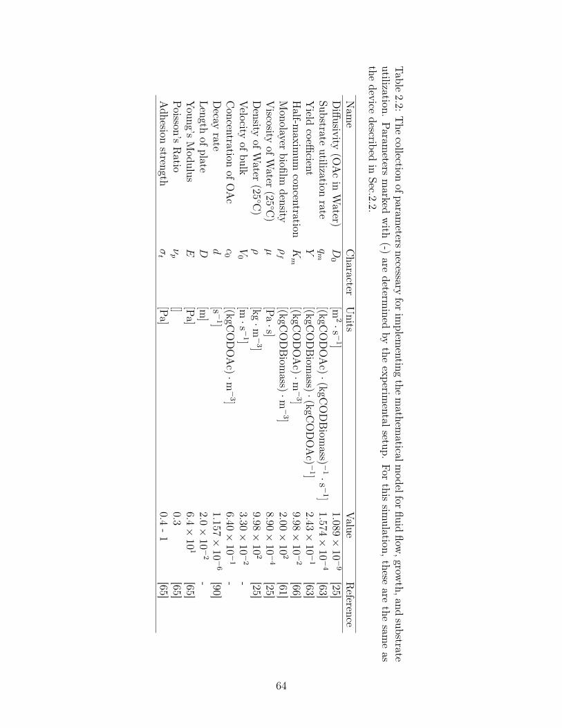
Table2.2:

The

collectionofparam

etersnecessary

forim

plementing

themathem

aticalmodelfor

fluidflow

,growth,and

substrateutilization.

Param

etersmarked

with

(-)are

determined

bythe

experimentalsetup.

Forthis

simulation,these

arethe

sameas

thedevice

describedin

Sec.2.2.

Nam

eCharacter

Units

Value

Reference

Diffusivity

(OAcin

Water)

D0

[m2·s −

1]1.089

×10−

9[25]

Substrateutilization

rateqm

[(kgC

OD

OA

c)·(kgC

OD

Biom

ass) −1·s −

1]1.574

×10−

4[63]

Yield

coefficient

Y[(k

gCO

DB

iomass)·(k

gCO

DO

Ac) −

1]2.43×

10−

1[63]

Half-m

aximum

concentrationKm

[(kgC

OD

OA

c)·m−

3]9.98×

10−

2[66]

Monolayer

biofilmdensity

ρf

[(kgC

OD

Biom

ass)·m−

3]2.00×

102

[61]Viscosity

ofWater

(25C

)µ

[Pa·s]

8.90×

10−

4[25]

Density

ofWater

(25C

)ρ

[kg·m−

3]9.98×

102

[25]Velocity

ofbulkV

0[m·s −

1]3.30×

10−

2-

Concentration

ofOAc

c0

[(kgC

OD

OA

c)·m−

3]6.40×

10−

1-

Decay

rated

[s −1]

1.157×

10−

6[90]

Lengthofplate

D[m

]2.0×

10−

2-

Young’s

Modulus

E[P

a]6.4×

101

[65]Poisson’s

Ratio

νp

[]0.3

[65]Adhesion

strengthσt

[Pa]

0.4-1

[65]

64

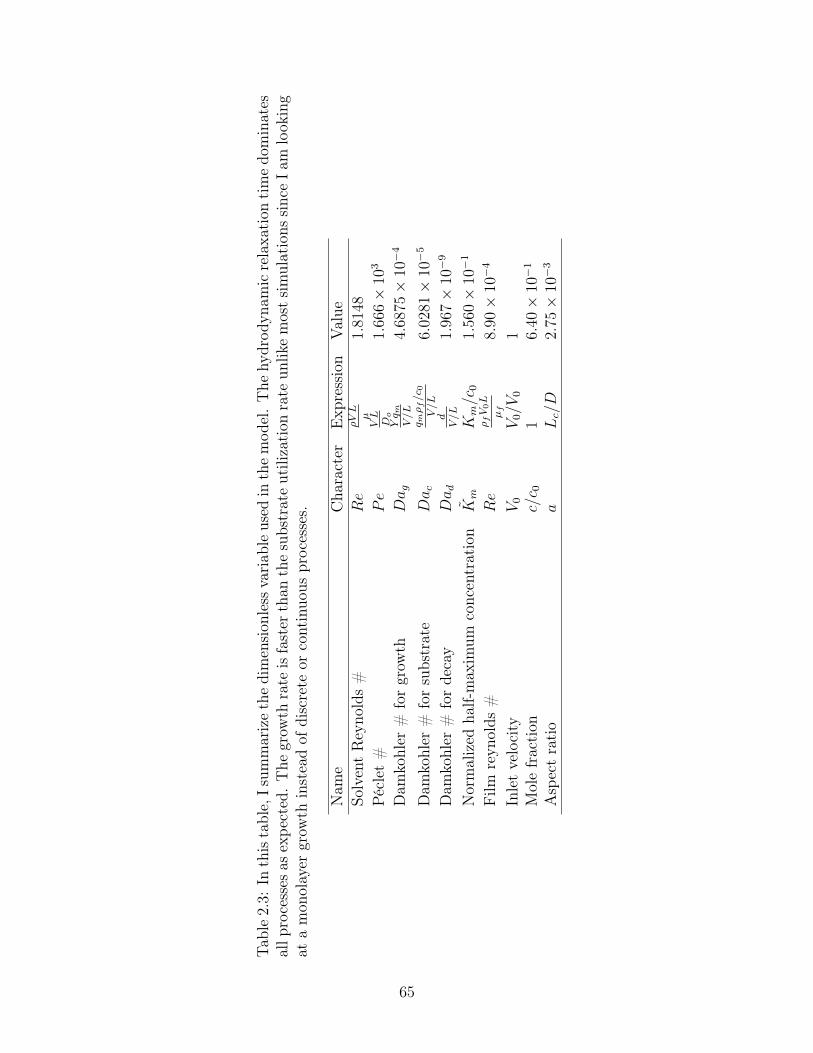
Table2.3:

Inthistable,Is

ummarizethedimension

less

variab

leused

inthemod

el.The

hydrod

ynam

icrelaxa

tion

timedo

minates

allp

rocesses

asexpe

cted.The

grow

thrate

isfaster

than

thesubstrateutilization

rate

unlik

emostsimulations

sinceIa

mlook

ing

atamon

olayer

grow

thinsteadof

discrete

orcontinuo

usprocesses.

Nam

eCha

racter

Exp

ression

Value

SolventReyno

lds#

Re

ρVLµ

1.81

48

Péclet#

Pe

VL

Do

1.66

6×

103

Dam

kohler

#forgrow

thDag

Yq m

V/L

4.68

75×

10−

4

Dam

kohler

#forsubstrate

Dac

q mρf/c 0

V/L

6.02

81×

10−

5

Dam

kohler

#fordecay

Dad

dV/L

1.96

7×

10−

9

Normalized

half-max

imum

concentration

Km

Km/c

01.

560×

10−

1

Film

reyn

olds

#Re

ρfV

0L

µf

8.90×

10−

4

Inletvelocity

V0

V0/V

01

Molefraction

c/c 0

16.

40×

10−

1

Aspectratio

aLc/D

2.75×

10−

3

65

THIS PAGE INTENTIONALLY LEFT BLANK

66

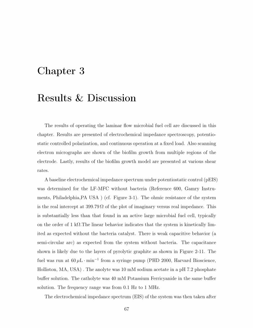
Chapter 3

Results & Discussion

The results of operating the laminar flow microbial fuel cell are discussed in this

chapter. Results are presented of electrochemical impedance spectroscopy, potentio-

static controlled polarization, and continuous operation at a fixed load. Also scanning

electron micrographs are shown of the biofilm growth from multiple regions of the

electrode. Lastly, results of the biofilm growth model are presented at various shear

rates.

A baseline electrochemical impedance spectrum under potentiostatic control (pEIS)

was determined for the LF-MFC without bacteria (Reference 600, Gamry Instru-

ments, Philadelphia,PA USA ) (cf. Figure 3-1). The ohmic resistance of the system

is the real intercept at 399.79 Ω of the plot of imaginary versus real impedance. This

is substantially less than that found in an active large microbial fuel cell, typically

on the order of 1 kΩ.The linear behavior indicates that the system is kinetically lim-

ited as expected without the bacteria catalyst. There is weak capacitive behavior (a

semi-circular arc) as expected from the system without bacteria. The capacitance

shown is likely due to the layers of pyrolytic graphite as shown in Figure 2-11. The

fuel was run at 60µL ·min−1 from a syringe pump (PHD 2000, Harvard Bioscience,

Holliston, MA, USA) . The anolyte was 10 mM sodium acetate in a pH 7.2 phosphate

buffer solution. The catholyte was 40 mM Potassium Ferricyanide in the same buffer

solution. The frequency range was from 0.1 Hz to 1 MHz.

The electrochemical impedance spectrum (EIS) of the system was then taken after

67

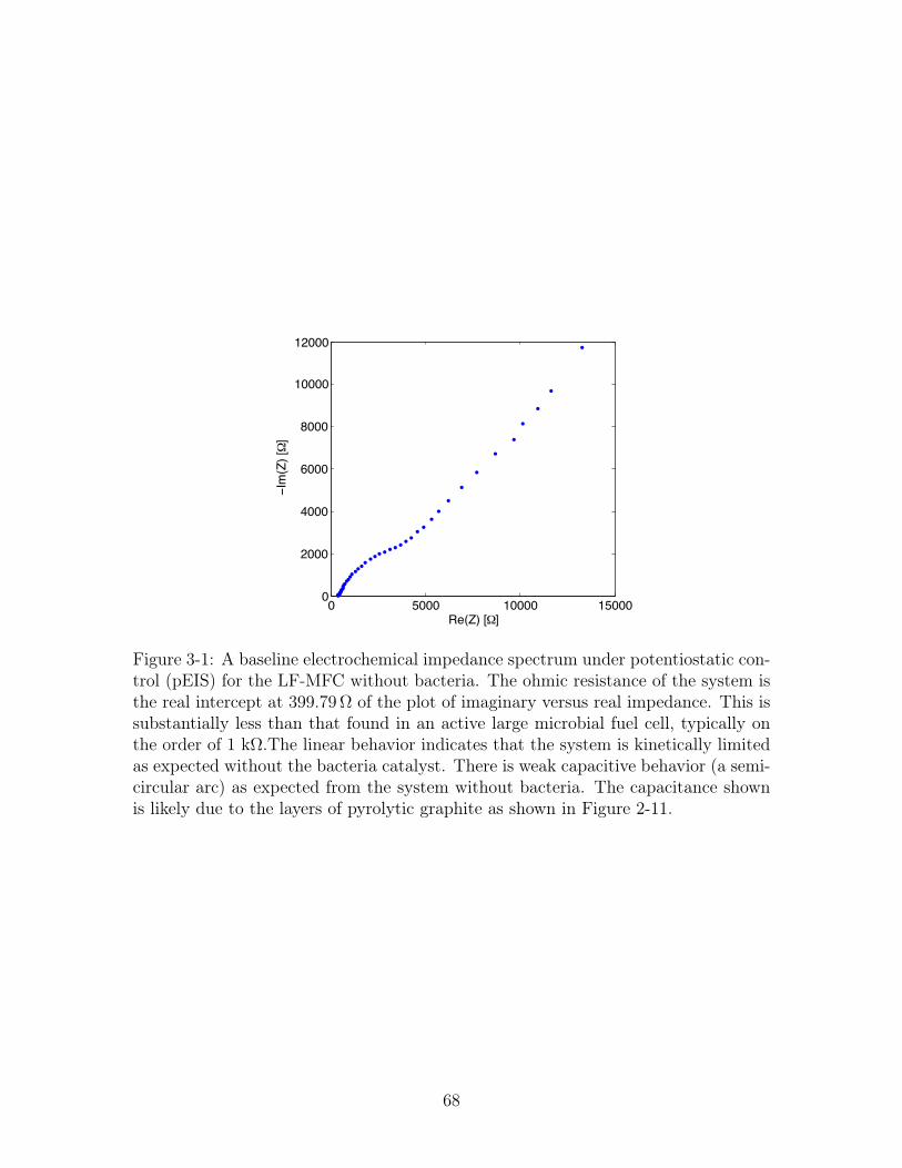
0 5000 10000 150000

2000

4000

6000

8000

10000

12000

Re(Z) [Ω]

−Im

(Z) [Ω

]

Figure 3-1: A baseline electrochemical impedance spectrum under potentiostatic con-trol (pEIS) for the LF-MFC without bacteria. The ohmic resistance of the system isthe real intercept at 399.79 Ω of the plot of imaginary versus real impedance. This issubstantially less than that found in an active large microbial fuel cell, typically onthe order of 1 kΩ.The linear behavior indicates that the system is kinetically limitedas expected without the bacteria catalyst. There is weak capacitive behavior (a semi-circular arc) as expected from the system without bacteria. The capacitance shownis likely due to the layers of pyrolytic graphite as shown in Figure 2-11.

68

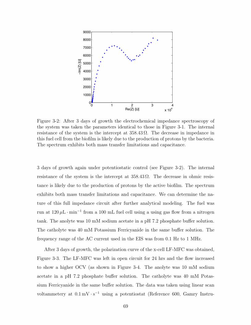
0 1 2 3 4x 104

0

1000

2000

3000

4000

5000

6000

7000

8000

9000

Re(Z) [Ω]

−Im

(Z) [Ω

]

Figure 3-2: After 3 days of growth the electrochemical impedance spectroscopy ofthe system was taken the parameters identical to those in Figure 3-1. The internalresistance of the system is the intercept at 358.43 Ω. The decrease in impedance inthis fuel cell from the biofilm is likely due to the production of protons by the bacteria.The spectrum exhibits both mass transfer limitations and capacitance.

3 days of growth again under potentiostatic control (see Figure 3-2). The internal

resistance of the system is the intercept at 358.43 Ω. The decrease in ohmic resis-

tance is likely due to the production of protons by the active biofilm. The spectrum

exhibits both mass transfer limitations and capacitance. We can determine the na-

ture of this full impedance circuit after further analytical modeling. The fuel was

run at 120µL ·min−1 from a 100 mL fuel cell using a using gas flow from a nitrogen

tank. The anolyte was 10 mM sodium acetate in a pH 7.2 phosphate buffer solution.

The catholyte was 40 mM Potassium Ferricyanide in the same buffer solution. The

frequency range of the AC current used in the EIS was from 0.1 Hz to 1 MHz.

After 3 days of growth, the polarization curve of the x-cell LF-MFC was obtained,

Figure 3-3. The LF-MFC was left in open circuit for 24 hrs and the flow increased

to show a higher OCV (as shown in Figure 3-4. The anolyte was 10 mM sodium

acetate in a pH 7.2 phosphate buffer solution. The catholyte was 40 mM Potas-

sium Ferricyanide in the same buffer solution. The data was taken using linear scan

voltammetery at 0.1 mV · s−1 using a potentiostat (Reference 600, Gamry Instru-

69

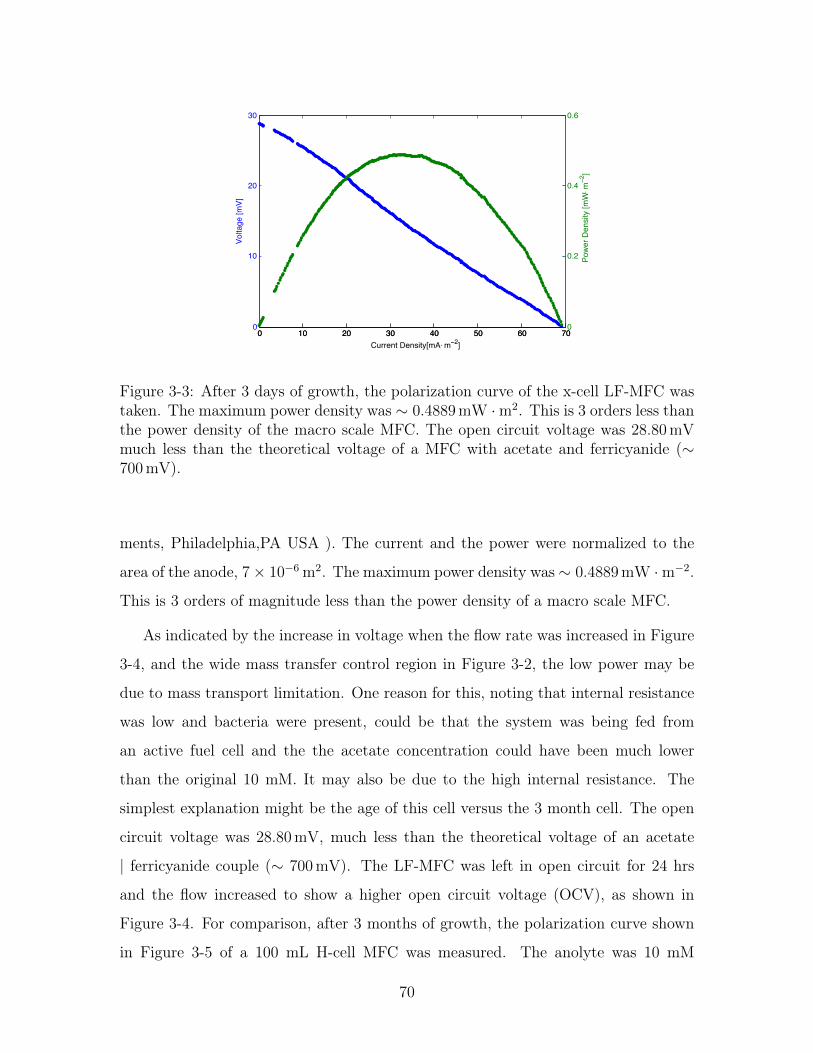
0 10 20 30 40 50 60 700

10

20

30

Current Density[mA⋅ m−2]

Volta

ge [m

V]

0 10 20 30 40 50 60 700

0.2

0.4

0.6

Pow

er D

ensi

ty [m

W⋅ m

−2]

Figure 3-3: After 3 days of growth, the polarization curve of the x-cell LF-MFC wastaken. The maximum power density was ∼ 0.4889 mW ·m2. This is 3 orders less thanthe power density of the macro scale MFC. The open circuit voltage was 28.80 mVmuch less than the theoretical voltage of a MFC with acetate and ferricyanide (∼700 mV).

ments, Philadelphia,PA USA ). The current and the power were normalized to the

area of the anode, 7× 10−6 m2. The maximum power density was∼ 0.4889 mW ·m−2.

This is 3 orders of magnitude less than the power density of a macro scale MFC.

As indicated by the increase in voltage when the flow rate was increased in Figure

3-4, and the wide mass transfer control region in Figure 3-2, the low power may be

due to mass transport limitation. One reason for this, noting that internal resistance

was low and bacteria were present, could be that the system was being fed from

an active fuel cell and the the acetate concentration could have been much lower

than the original 10 mM. It may also be due to the high internal resistance. The

simplest explanation might be the age of this cell versus the 3 month cell. The open

circuit voltage was 28.80 mV, much less than the theoretical voltage of an acetate

| ferricyanide couple (∼ 700 mV). The LF-MFC was left in open circuit for 24 hrs

and the flow increased to show a higher open circuit voltage (OCV), as shown in

Figure 3-4. For comparison, after 3 months of growth, the polarization curve shown

in Figure 3-5 of a 100 mL H-cell MFC was measured. The anolyte was 10 mM

70

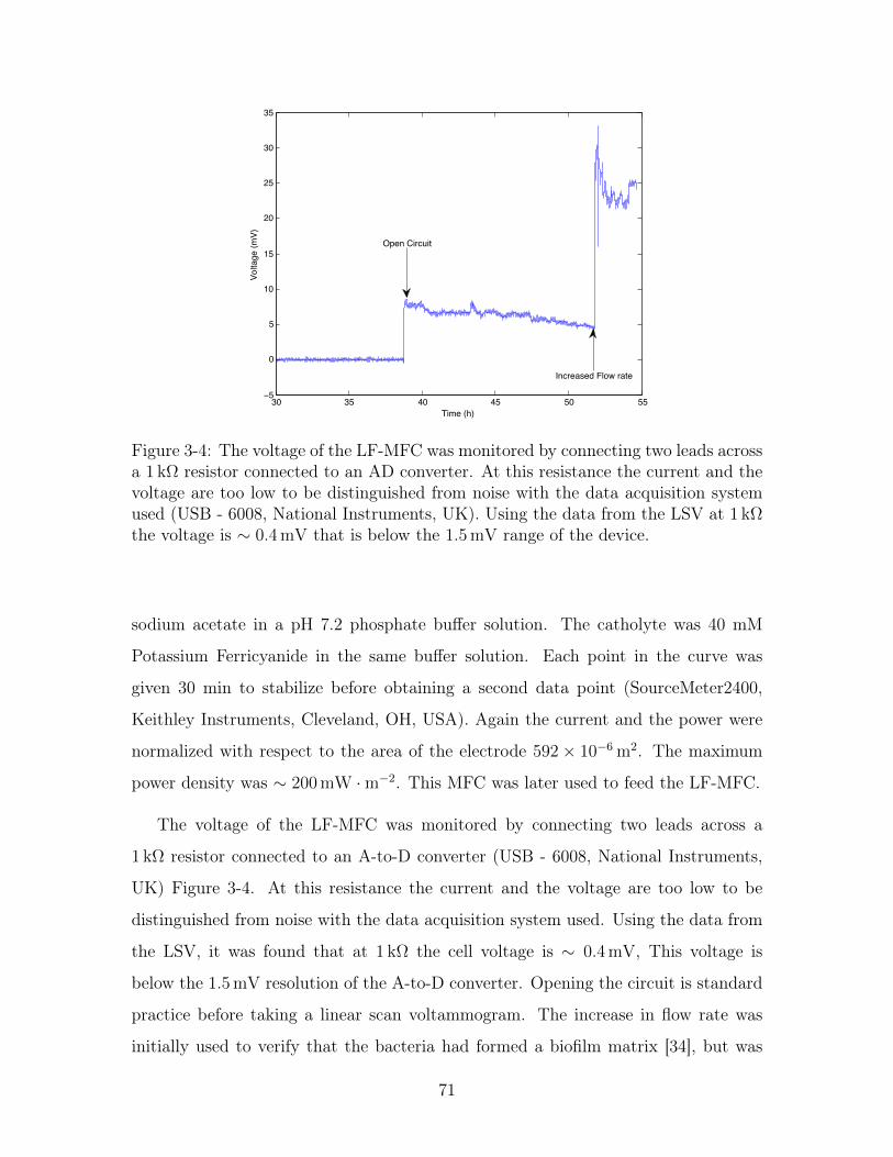
30 35 40 45 50 55−5

0

5

10

15

20

25

30

35

Time (h)

Volta

ge (m

V)Open Circuit

Increased Flow rate

Figure 3-4: The voltage of the LF-MFC was monitored by connecting two leads acrossa 1 kΩ resistor connected to an AD converter. At this resistance the current and thevoltage are too low to be distinguished from noise with the data acquisition systemused (USB - 6008, National Instruments, UK). Using the data from the LSV at 1 kΩthe voltage is ∼ 0.4 mV that is below the 1.5 mV range of the device.

sodium acetate in a pH 7.2 phosphate buffer solution. The catholyte was 40 mM

Potassium Ferricyanide in the same buffer solution. Each point in the curve was

given 30 min to stabilize before obtaining a second data point (SourceMeter2400,

Keithley Instruments, Cleveland, OH, USA). Again the current and the power were

normalized with respect to the area of the electrode 592× 10−6 m2. The maximum

power density was ∼ 200 mW ·m−2. This MFC was later used to feed the LF-MFC.

The voltage of the LF-MFC was monitored by connecting two leads across a

1 kΩ resistor connected to an A-to-D converter (USB - 6008, National Instruments,

UK) Figure 3-4. At this resistance the current and the voltage are too low to be

distinguished from noise with the data acquisition system used. Using the data from

the LSV, it was found that at 1 kΩ the cell voltage is ∼ 0.4 mV, This voltage is

below the 1.5 mV resolution of the A-to-D converter. Opening the circuit is standard

practice before taking a linear scan voltammogram. The increase in flow rate was

initially used to verify that the bacteria had formed a biofilm matrix [34], but was

71

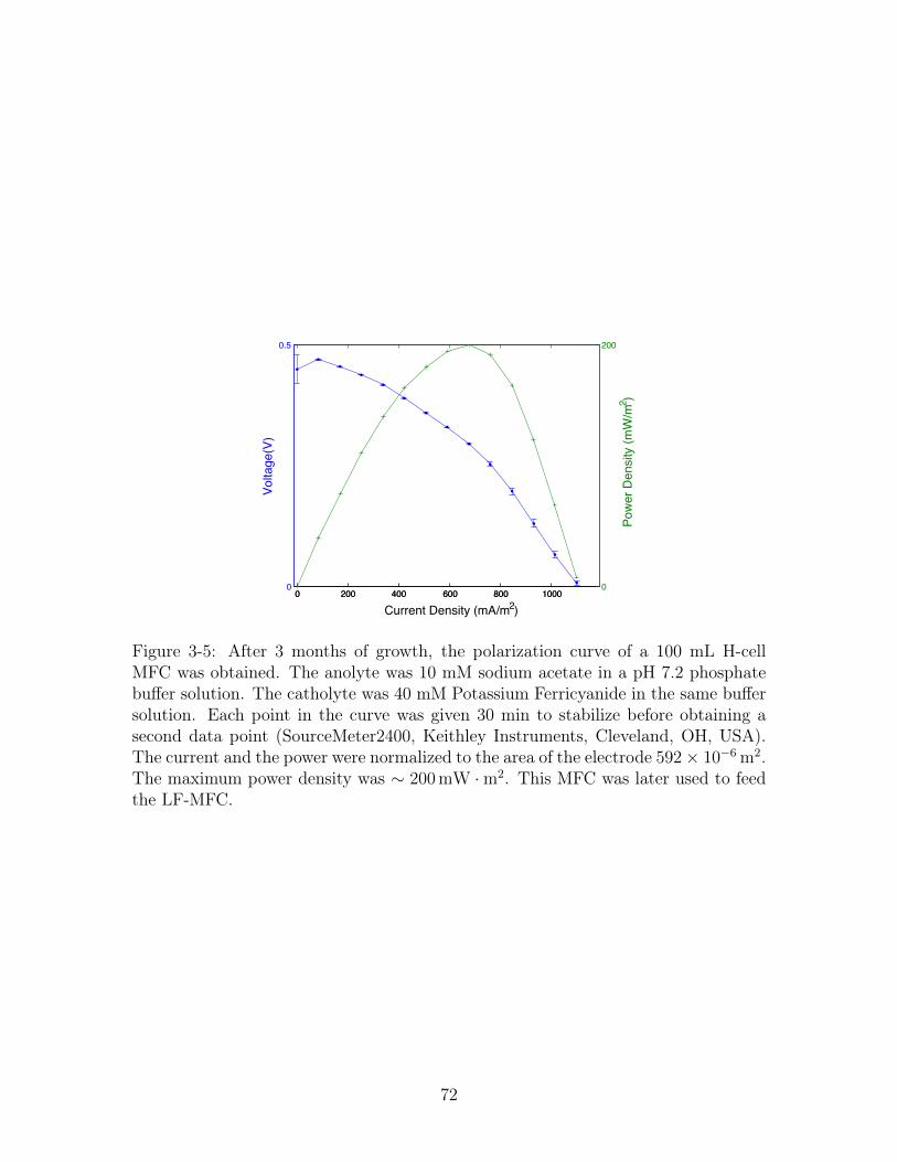
0 200 400 600 800 10000

0.5

Volta

ge(V

)

Current Density (mA/m2)0 200 400 600 800 1000

0

200

Pow

er D

ensi

ty (m

W/m

2 )

Figure 3-5: After 3 months of growth, the polarization curve of a 100 mL H-cellMFC was obtained. The anolyte was 10 mM sodium acetate in a pH 7.2 phosphatebuffer solution. The catholyte was 40 mM Potassium Ferricyanide in the same buffersolution. Each point in the curve was given 30 min to stabilize before obtaining asecond data point (SourceMeter2400, Keithley Instruments, Cleveland, OH, USA).The current and the power were normalized to the area of the electrode 592× 10−6 m2.The maximum power density was ∼ 200 mW ·m2. This MFC was later used to feedthe LF-MFC.

72

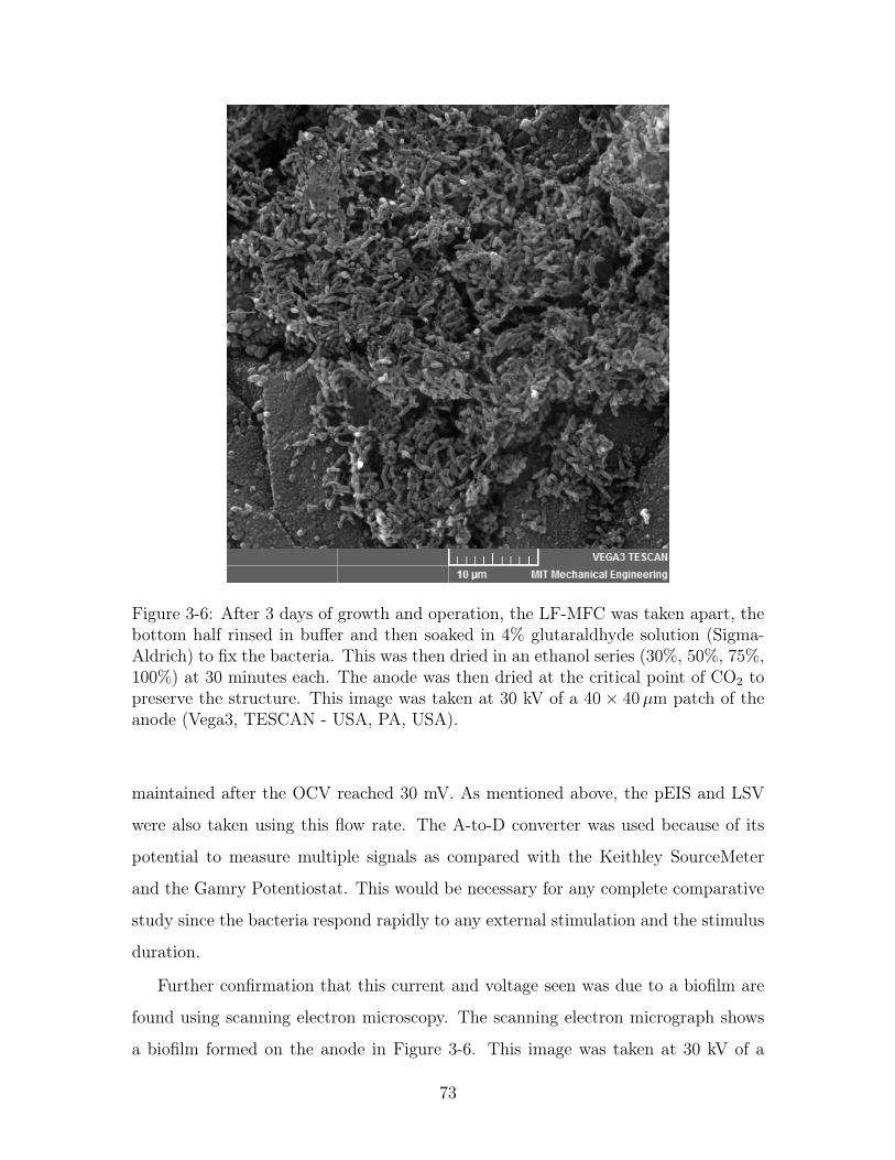
Figure 3-6: After 3 days of growth and operation, the LF-MFC was taken apart, thebottom half rinsed in buffer and then soaked in 4% glutaraldhyde solution (Sigma-Aldrich) to fix the bacteria. This was then dried in an ethanol series (30%, 50%, 75%,100%) at 30 minutes each. The anode was then dried at the critical point of CO2 topreserve the structure. This image was taken at 30 kV of a 40× 40µm patch of theanode (Vega3, TESCAN - USA, PA, USA).

maintained after the OCV reached 30 mV. As mentioned above, the pEIS and LSV

were also taken using this flow rate. The A-to-D converter was used because of its

potential to measure multiple signals as compared with the Keithley SourceMeter

and the Gamry Potentiostat. This would be necessary for any complete comparative

study since the bacteria respond rapidly to any external stimulation and the stimulus

duration.

Further confirmation that this current and voltage seen was due to a biofilm are

found using scanning electron microscopy. The scanning electron micrograph shows

a biofilm formed on the anode in Figure 3-6. This image was taken at 30 kV of a

73

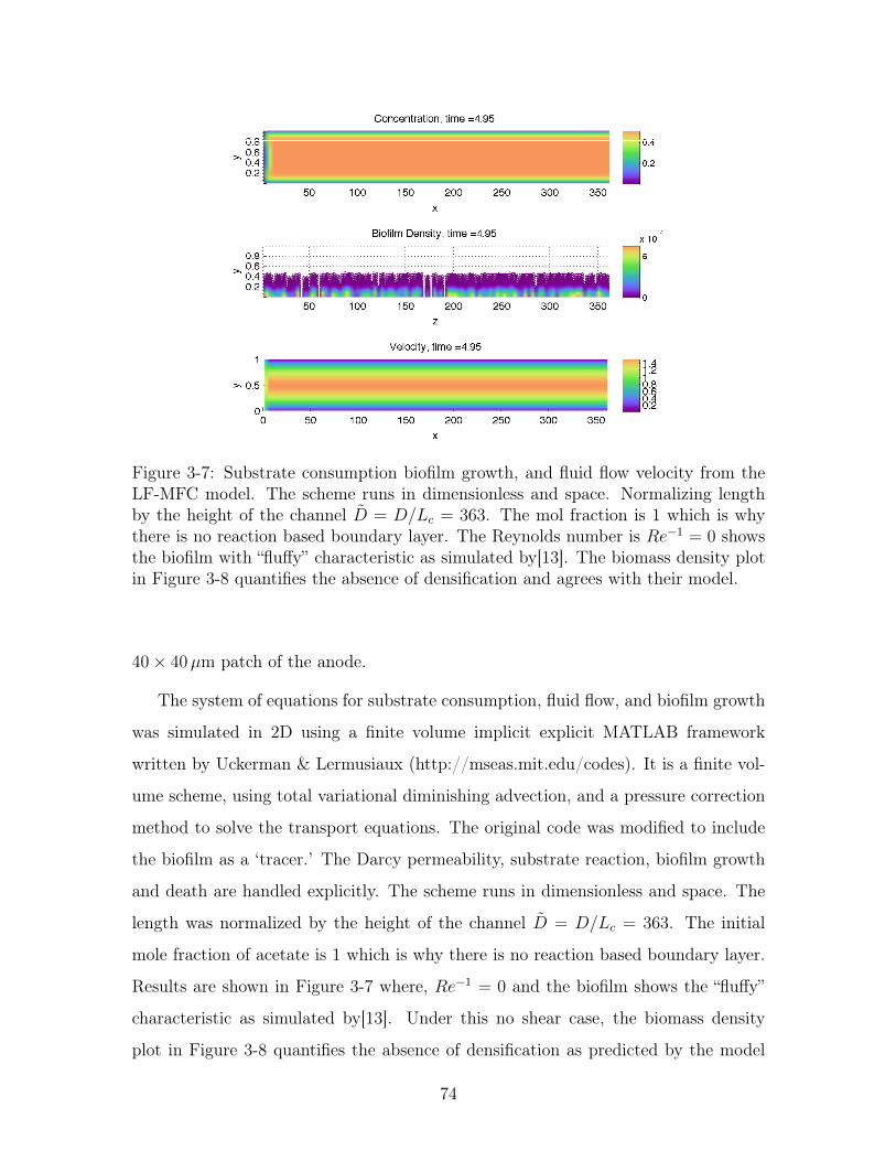
Figure 3-7: Substrate consumption biofilm growth, and fluid flow velocity from theLF-MFC model. The scheme runs in dimensionless and space. Normalizing lengthby the height of the channel D = D/Lc = 363. The mol fraction is 1 which is whythere is no reaction based boundary layer. The Reynolds number is Re−1 = 0 showsthe biofilm with “fluffy” characteristic as simulated by[13]. The biomass density plotin Figure 3-8 quantifies the absence of densification and agrees with their model.

40× 40µm patch of the anode.

The system of equations for substrate consumption, fluid flow, and biofilm growth

was simulated in 2D using a finite volume implicit explicit MATLAB framework

written by Uckerman & Lermusiaux (http://mseas.mit.edu/codes). It is a finite vol-

ume scheme, using total variational diminishing advection, and a pressure correction

method to solve the transport equations. The original code was modified to include

the biofilm as a ‘tracer.’ The Darcy permeability, substrate reaction, biofilm growth

and death are handled explicitly. The scheme runs in dimensionless and space. The

length was normalized by the height of the channel D = D/Lc = 363. The initial

mole fraction of acetate is 1 which is why there is no reaction based boundary layer.

Results are shown in Figure 3-7 where, Re−1 = 0 and the biofilm shows the “fluffy”

characteristic as simulated by[13]. Under this no shear case, the biomass density

plot in Figure 3-8 quantifies the absence of densification as predicted by the model

74

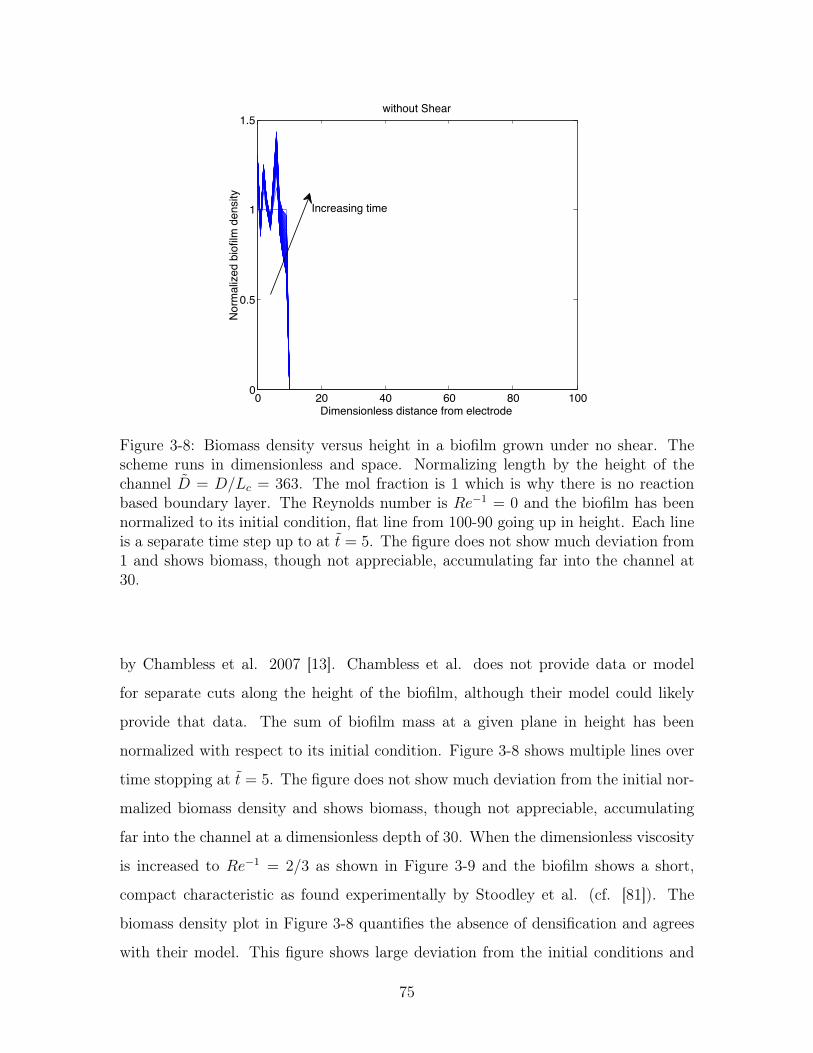
1008060402000

0.5

1

1.5without Shear

Nor

mal

ized

bio

film

den

sity

Dimensionless distance from electrode

Increasing time

Figure 3-8: Biomass density versus height in a biofilm grown under no shear. Thescheme runs in dimensionless and space. Normalizing length by the height of thechannel D = D/Lc = 363. The mol fraction is 1 which is why there is no reactionbased boundary layer. The Reynolds number is Re−1 = 0 and the biofilm has beennormalized to its initial condition, flat line from 100-90 going up in height. Each lineis a separate time step up to at t = 5. The figure does not show much deviation from1 and shows biomass, though not appreciable, accumulating far into the channel at30.

by Chambless et al. 2007 [13]. Chambless et al. does not provide data or model

for separate cuts along the height of the biofilm, although their model could likely

provide that data. The sum of biofilm mass at a given plane in height has been

normalized with respect to its initial condition. Figure 3-8 shows multiple lines over

time stopping at t = 5. The figure does not show much deviation from the initial nor-

malized biomass density and shows biomass, though not appreciable, accumulating

far into the channel at a dimensionless depth of 30. When the dimensionless viscosity

is increased to Re−1 = 2/3 as shown in Figure 3-9 and the biofilm shows a short,

compact characteristic as found experimentally by Stoodley et al. (cf. [81]). The

biomass density plot in Figure 3-8 quantifies the absence of densification and agrees

with their model. This figure shows large deviation from the initial conditions and

75

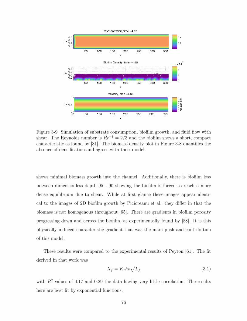
Figure 3-9: Simulation of substrate consumption, biofilm growth, and fluid flow withshear. The Reynolds number is Re−1 = 2/3 and the biofilm shows a short, compactcharacteristic as found by [81]. The biomass density plot in Figure 3-8 quantifies theabsence of densification and agrees with their model.

shows minimal biomass growth into the channel. Additionally, there is biofilm loss

between dimensionless depth 95 - 90 showing the biofilm is forced to reach a more

dense equilibrium due to shear. While at first glance these images appear identi-

cal to the images of 2D biofilm growth by Picioreanu et al. they differ in that the

biomass is not homogenous throughout [65]. There are gradients in biofilm porosity

progressing down and across the biofilm, as experimentally found by [88]. It is this

physically induced characteristic gradient that was the main push and contribution

of this model.

These results were compared to the experimental results of Peyton [61]. The fit

derived in that work was

Xf = Krho√Lf (3.1)

with R2 values of 0.17 and 0.29 the data having very little correlation. The results

here are best fit by exponential functions,

76

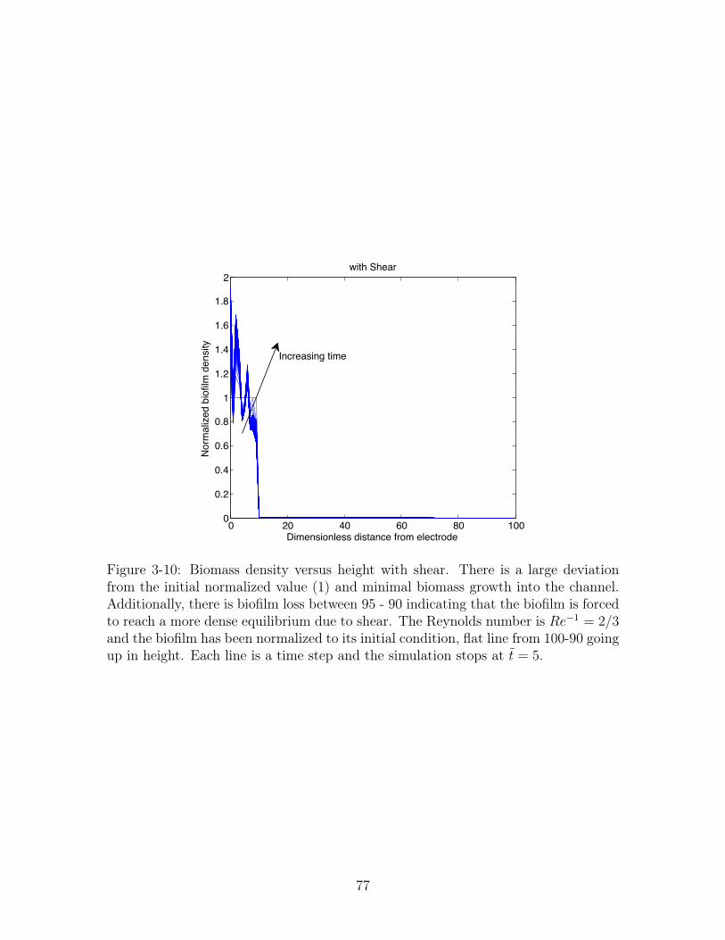
1008060402000

0.2

0.4

0.6

0.8

1

1.2

1.4

1.6

1.8

2with Shear

Dimensionless distance from electrode

Nor

mal

ized

bio

film

den

sity

Increasing time

Figure 3-10: Biomass density versus height with shear. There is a large deviationfrom the initial normalized value (1) and minimal biomass growth into the channel.Additionally, there is biofilm loss between 95 - 90 indicating that the biofilm is forcedto reach a more dense equilibrium due to shear. The Reynolds number is Re−1 = 2/3and the biofilm has been normalized to its initial condition, flat line from 100-90 goingup in height. Each line is a time step and the simulation stops at t = 5.

77

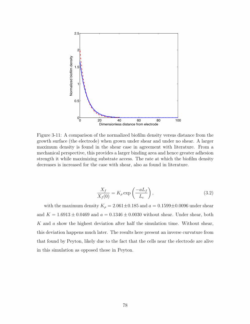
0 20 40 60 80 1000

0.5

1

1.5

2

2.5

Dimensionless distance from electrode

Nor

mal

ized

bio

film

den

sity

Figure 3-11: A comparison of the normalized biofilm density versus distance from thegrowth surface (the electrode) when grown under shear and under no shear. A largermaximum density is found in the shear case in agreement with literature. From amechanical perspective, this provides a larger binding area and hence greater adhesionstrength it while maximizing substrate access. The rate at which the biofilm densitydecreases is increased for the case with shear, also as found in literature.

Xf

Xf (0)= Kρ exp

(−aLfLc

), (3.2)

with the maximum densityKρ = 2.061±0.185 and a = 0.1599±0.0096 under shear

and K = 1.6913± 0.0469 and a = 0.1346± 0.0030 without shear. Under shear, both

K and a show the highest deviation after half the simulation time. Without shear,

this deviation happens much later. The results here present an inverse curvature from

that found by Peyton, likely due to the fact that the cells near the electrode are alive

in this simulation as opposed those in Peyton.

78

Chapter 4

Conclusion & Future Work

Biofilms are communities of bacteria that respond dynamically to varying envi-

ronmental stresses. A more complete understanding of biofilms will help us more

efficiently grow them in microbial fuel cells or remove them from the human body.

The tools that we have to study them are beginning to scale down from large reactors

and beakers to length scales where we can see how biofilms’ response at their time

scale. The models of biofilm behavior and our ability to solve 3D coupled models

are beginning to explain some of the phenomena surrounding the biofilms response

to chemical stresses. We must now begin to look at how they respond to mechanical

stresses with our new tools.

A new tool to study biofilms was developed in this thesis: a Laminar-Flow Micro-

bial Fuel Cell (LF-MFC). Similarly a more complete model of biofilm growth under

hydrodynamic control was developed. The device was designed to be compatible with

conditions for biofilm growth and amenable to the use of light and confocal microscopy

for direct measurement of the growing biofilm by using acrylic as the working ma-

terial instead of other commonly used materials for microfluidcs, like poly(dimethyl

siloxane). Machinist parameters were created to improve micro-machining not only

for this device, but also other microfludic devices milled from acrylic.The device is

more biocompatible than traditional lithographic electrodes and enables the use of

more relevant materials by using solid-type electrodes. The 3-outlet design allows for

more accurate indirect measurements of biofilm health including: substrate utiliza-

79

tion (chemical oxygen demand measurement), and pH change. The device is designed

to measure total current and potential as a functional microbial fuel cell and another

indirect measurement of biofilm health. The device tested with one type of electrode

and one flow rate. Preliminary data is presented to guide further experiments on

biofilm substrate compatibility, a biofilms response to shear, and the optimization of

a microbial fuel cell.

A model has been developed that incorporates biofilm growth from a continuous

perspective. The model constructed is not steady-state in either fluid flow or biofilm

growth so that the evolution of all boundary layers, hydrodynamic, concentration, and

biomass, can be observed. The biofilm’s response to shear stress is explored where

the biofilm is modeled as a poroelastic medium. Previous biofilm models (cf. Sec.

1.4) incorporated shear stress as a parametric constraint on external areas exposed

to shear. Older models did not include flow through the biofilm, assuming it was

negligible. The impact of shear stress in this model is only one part of the fluid

flow that affects the porosity through the overall geometry and connectedness of the

biofilm. Simulations at different shear rates tests not only reveal similar structure to

previous models that included shear, but also begin to show some of the anisotropic

structure that is characteristic of real world biofilms.

With the LF-MFC, future studies will be done to determine the impact of material

chemistry on biofilm adhesion, formation and metabolism. This study will be guided

by the free energy model mentioned in Sec. 2.2.3. The biofilms response to shear will

be studied experimentally and numerically by varying the shear rate in the LF-MFC

to test the hypothesis that a biofilm is a dynamic poroelastic medium as used in the

model.

80

Appendix A

Machinist Parameters for a Laminar

Flow - Microbial Fuel Cell

Tool parameters and setup have been optimized to yield a smooth surface finish

and preserve flow geometry. It is recommended that any machining of a microfluidic

device with similar parameters be done with similar.

All mill paths were and G-code was generated using MasterCam X5. The tool

paths chosen for the channels was a “2D pocket Dynamic Area Mill.” This produced

an optimal path for hugging corners. A stepover of 5% diameter was used to minimize

scalloping. Scalloping can also be reduced by using a finish pass. Since the depth of

cut for this part is 55µm, any finish pass would produce nanometer sized chips that

could not be properly cleared with flood coolant. Atomized coolant is recommended

for clearing the small chips in micro-machining to improve surface finish, minimize

tool wear and part temperature the latter that can cause welding of chips to the part

[31]. The mill used here is not equipped for that but the measured surface finish is

at ∼ 100 nm which is acceptable. Optimization of the cutting parameters matched

the formula found by Vogler et al,

Ra ∝CL2

0.5D

with a proportionality constant of 5 for acrylic [89].The path for the conductive tape,

81

electrical connectors was a parallel spiral without overlap since surface finish did not

matter and a single spring pass of 10µm. The spring pass is necessary for the pockets

and kept for consistency. The pockets were similarly milled using a parallel spiral

pass without overlap in one pass to a depth of 100µm for the carbon tape.

All parts were cut on a Microlution 363-S (Microlution, Chicago, IL, USA). This

mill is equipped with a 56,000 rpm, air-turbine spindle with a 3.175 mm (1/8”) dia

chuck, flood coolant and air coolant. The pallet working area is 60 × 58 mm(x × y)

and a custom fixture was made to hold each part in place to preserve alignment. The

rotational velocity was limited to 48,000 rpm to minimize wear on spindle bearings.

The channels were cut using a 0.254 mm (0.01”) 4 flute end mill. This was chosen

over smaller end mills and 2 flute end mills to minimize scalloping. The chip load

was 1.9µ/tooth which gave a feed rate of 365 mm/min.

82

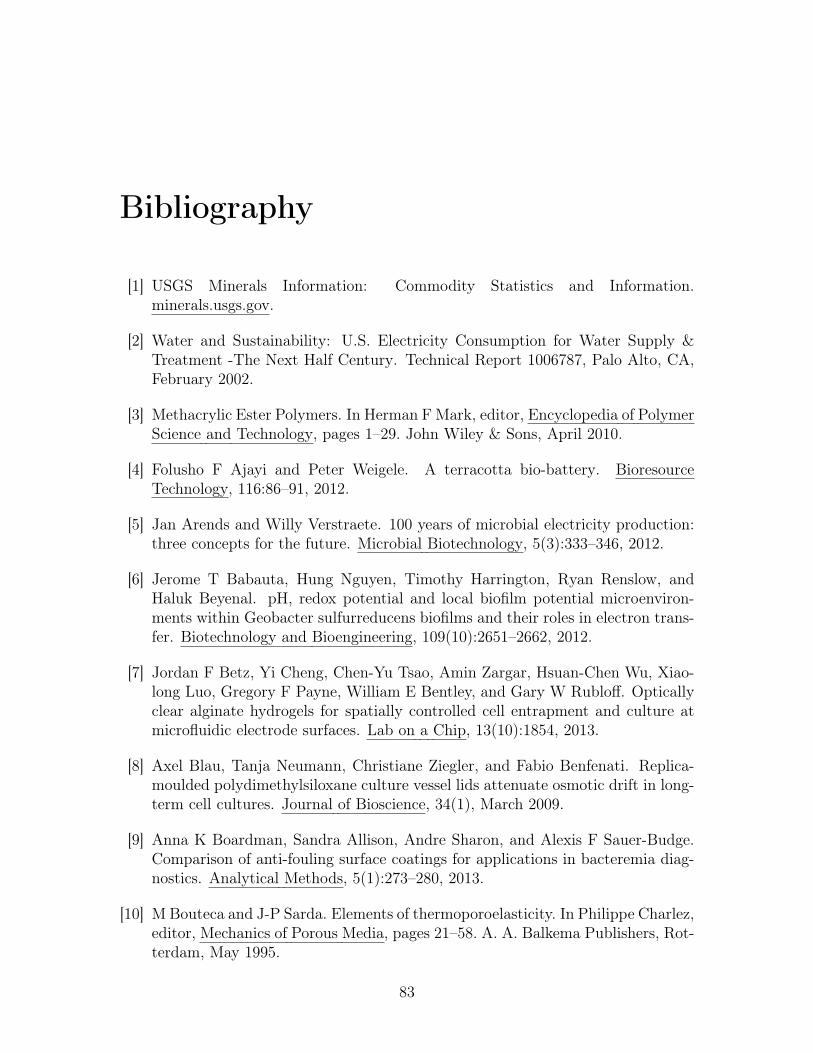
Bibliography

[1] USGS Minerals Information: Commodity Statistics and Information.minerals.usgs.gov.

[2] Water and Sustainability: U.S. Electricity Consumption for Water Supply &Treatment -The Next Half Century. Technical Report 1006787, Palo Alto, CA,February 2002.

[3] Methacrylic Ester Polymers. In Herman F Mark, editor, Encyclopedia of PolymerScience and Technology, pages 1–29. John Wiley & Sons, April 2010.

[4] Folusho F Ajayi and Peter Weigele. A terracotta bio-battery. BioresourceTechnology, 116:86–91, 2012.

[5] Jan Arends and Willy Verstraete. 100 years of microbial electricity production:three concepts for the future. Microbial Biotechnology, 5(3):333–346, 2012.

[6] Jerome T Babauta, Hung Nguyen, Timothy Harrington, Ryan Renslow, andHaluk Beyenal. pH, redox potential and local biofilm potential microenviron-ments within Geobacter sulfurreducens biofilms and their roles in electron trans-fer. Biotechnology and Bioengineering, 109(10):2651–2662, 2012.

[7] Jordan F Betz, Yi Cheng, Chen-Yu Tsao, Amin Zargar, Hsuan-Chen Wu, Xiao-long Luo, Gregory F Payne, William E Bentley, and Gary W Rubloff. Opticallyclear alginate hydrogels for spatially controlled cell entrapment and culture atmicrofluidic electrode surfaces. Lab on a Chip, 13(10):1854, 2013.

[8] Axel Blau, Tanja Neumann, Christiane Ziegler, and Fabio Benfenati. Replica-moulded polydimethylsiloxane culture vessel lids attenuate osmotic drift in long-term cell cultures. Journal of Bioscience, 34(1), March 2009.

[9] Anna K Boardman, Sandra Allison, Andre Sharon, and Alexis F Sauer-Budge.Comparison of anti-fouling surface coatings for applications in bacteremia diag-nostics. Analytical Methods, 5(1):273–280, 2013.

[10] M Bouteca and J-P Sarda. Elements of thermoporoelasticity. In Philippe Charlez,editor, Mechanics of Porous Media, pages 21–58. A. A. Balkema Publishers, Rot-terdam, May 1995.

83

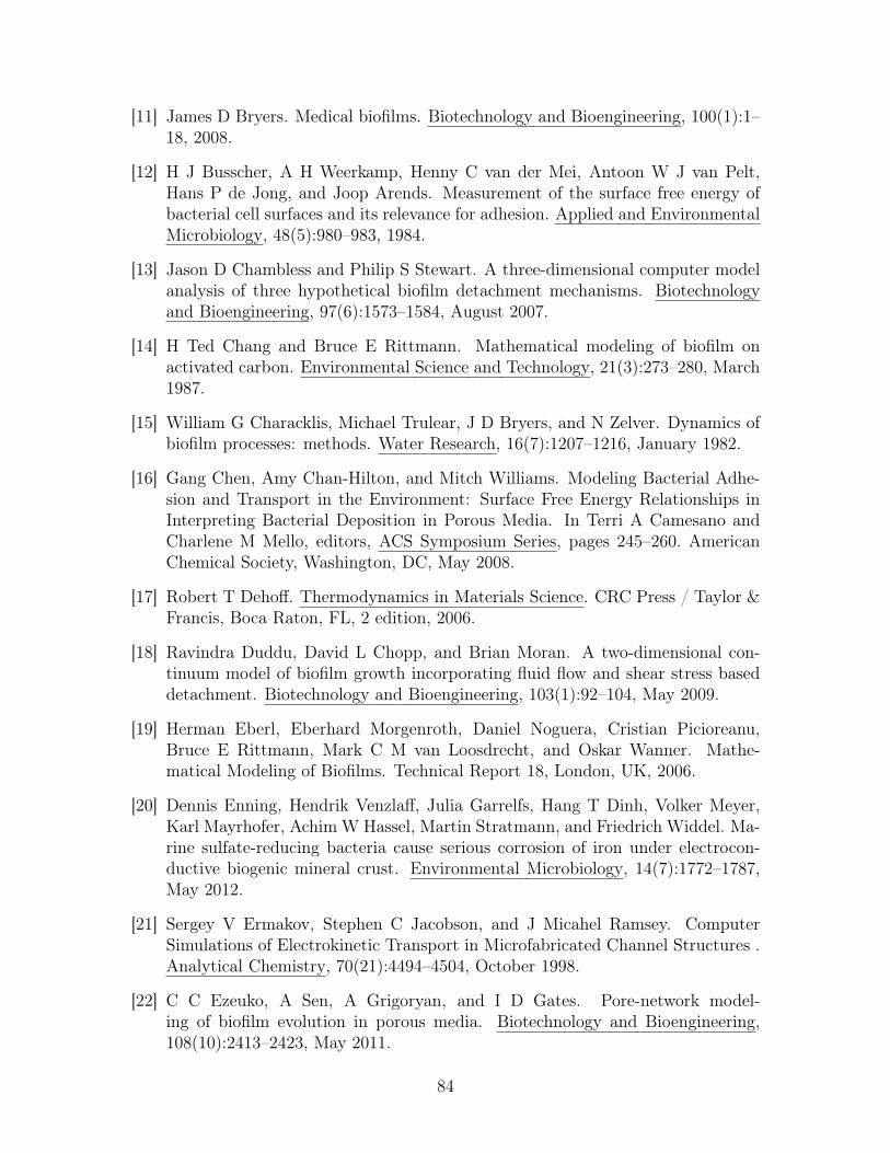
[11] James D Bryers. Medical biofilms. Biotechnology and Bioengineering, 100(1):1–18, 2008.

[12] H J Busscher, A H Weerkamp, Henny C van der Mei, Antoon W J van Pelt,Hans P de Jong, and Joop Arends. Measurement of the surface free energy ofbacterial cell surfaces and its relevance for adhesion. Applied and EnvironmentalMicrobiology, 48(5):980–983, 1984.

[13] Jason D Chambless and Philip S Stewart. A three-dimensional computer modelanalysis of three hypothetical biofilm detachment mechanisms. Biotechnologyand Bioengineering, 97(6):1573–1584, August 2007.

[14] H Ted Chang and Bruce E Rittmann. Mathematical modeling of biofilm onactivated carbon. Environmental Science and Technology, 21(3):273–280, March1987.

[15] William G Characklis, Michael Trulear, J D Bryers, and N Zelver. Dynamics ofbiofilm processes: methods. Water Research, 16(7):1207–1216, January 1982.

[16] Gang Chen, Amy Chan-Hilton, and Mitch Williams. Modeling Bacterial Adhe-sion and Transport in the Environment: Surface Free Energy Relationships inInterpreting Bacterial Deposition in Porous Media. In Terri A Camesano andCharlene M Mello, editors, ACS Symposium Series, pages 245–260. AmericanChemical Society, Washington, DC, May 2008.

[17] Robert T Dehoff. Thermodynamics in Materials Science. CRC Press / Taylor &Francis, Boca Raton, FL, 2 edition, 2006.

[18] Ravindra Duddu, David L Chopp, and Brian Moran. A two-dimensional con-tinuum model of biofilm growth incorporating fluid flow and shear stress baseddetachment. Biotechnology and Bioengineering, 103(1):92–104, May 2009.

[19] Herman Eberl, Eberhard Morgenroth, Daniel Noguera, Cristian Picioreanu,Bruce E Rittmann, Mark C M van Loosdrecht, and Oskar Wanner. Mathe-matical Modeling of Biofilms. Technical Report 18, London, UK, 2006.

[20] Dennis Enning, Hendrik Venzlaff, Julia Garrelfs, Hang T Dinh, Volker Meyer,Karl Mayrhofer, Achim W Hassel, Martin Stratmann, and Friedrich Widdel. Ma-rine sulfate-reducing bacteria cause serious corrosion of iron under electrocon-ductive biogenic mineral crust. Environmental Microbiology, 14(7):1772–1787,May 2012.

[21] Sergey V Ermakov, Stephen C Jacobson, and J Micahel Ramsey. ComputerSimulations of Electrokinetic Transport in Microfabricated Channel Structures .Analytical Chemistry, 70(21):4494–4504, October 1998.

[22] C C Ezeuko, A Sen, A Grigoryan, and I D Gates. Pore-network model-ing of biofilm evolution in porous media. Biotechnology and Bioengineering,108(10):2413–2423, May 2011.

84

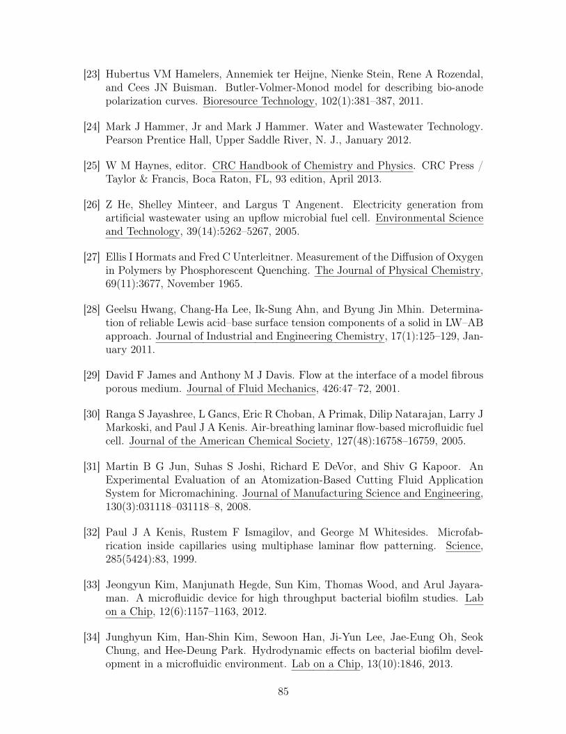
[23] Hubertus VM Hamelers, Annemiek ter Heijne, Nienke Stein, Rene A Rozendal,and Cees JN Buisman. Butler-Volmer-Monod model for describing bio-anodepolarization curves. Bioresource Technology, 102(1):381–387, 2011.

[24] Mark J Hammer, Jr and Mark J Hammer. Water and Wastewater Technology.Pearson Prentice Hall, Upper Saddle River, N. J., January 2012.

[25] W M Haynes, editor. CRC Handbook of Chemistry and Physics. CRC Press /Taylor & Francis, Boca Raton, FL, 93 edition, April 2013.

[26] Z He, Shelley Minteer, and Largus T Angenent. Electricity generation fromartificial wastewater using an upflow microbial fuel cell. Environmental Scienceand Technology, 39(14):5262–5267, 2005.

[27] Ellis I Hormats and Fred C Unterleitner. Measurement of the Diffusion of Oxygenin Polymers by Phosphorescent Quenching. The Journal of Physical Chemistry,69(11):3677, November 1965.

[28] Geelsu Hwang, Chang-Ha Lee, Ik-Sung Ahn, and Byung Jin Mhin. Determina-tion of reliable Lewis acid–base surface tension components of a solid in LW–ABapproach. Journal of Industrial and Engineering Chemistry, 17(1):125–129, Jan-uary 2011.

[29] David F James and Anthony M J Davis. Flow at the interface of a model fibrousporous medium. Journal of Fluid Mechanics, 426:47–72, 2001.

[30] Ranga S Jayashree, L Gancs, Eric R Choban, A Primak, Dilip Natarajan, Larry JMarkoski, and Paul J A Kenis. Air-breathing laminar flow-based microfluidic fuelcell. Journal of the American Chemical Society, 127(48):16758–16759, 2005.

[31] Martin B G Jun, Suhas S Joshi, Richard E DeVor, and Shiv G Kapoor. AnExperimental Evaluation of an Atomization-Based Cutting Fluid ApplicationSystem for Micromachining. Journal of Manufacturing Science and Engineering,130(3):031118–031118–8, 2008.

[32] Paul J A Kenis, Rustem F Ismagilov, and George M Whitesides. Microfab-rication inside capillaries using multiphase laminar flow patterning. Science,285(5424):83, 1999.

[33] Jeongyun Kim, Manjunath Hegde, Sun Kim, Thomas Wood, and Arul Jayara-man. A microfluidic device for high throughput bacterial biofilm studies. Labon a Chip, 12(6):1157–1163, 2012.

[34] Junghyun Kim, Han-Shin Kim, Sewoon Han, Ji-Yun Lee, Jae-Eung Oh, SeokChung, and Hee-Deung Park. Hydrodynamic effects on bacterial biofilm devel-opment in a microfluidic environment. Lab on a Chip, 13(10):1846, 2013.

85

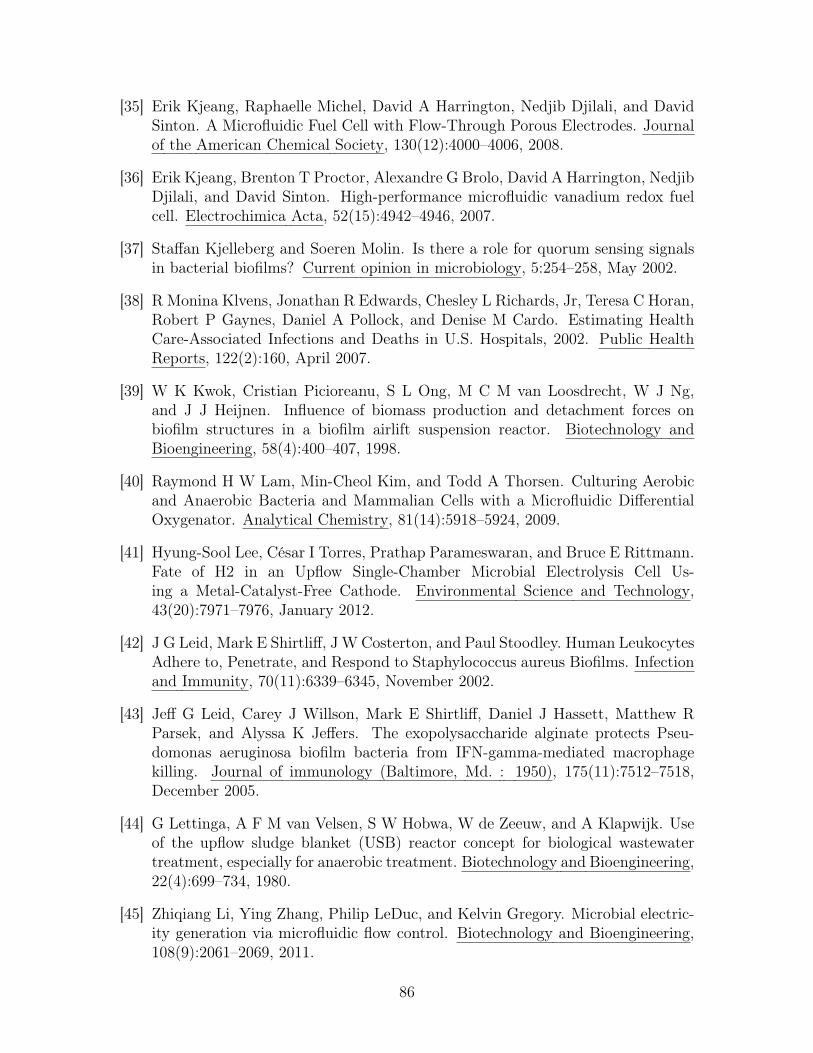
[35] Erik Kjeang, Raphaelle Michel, David A Harrington, Nedjib Djilali, and DavidSinton. A Microfluidic Fuel Cell with Flow-Through Porous Electrodes. Journalof the American Chemical Society, 130(12):4000–4006, 2008.

[36] Erik Kjeang, Brenton T Proctor, Alexandre G Brolo, David A Harrington, NedjibDjilali, and David Sinton. High-performance microfluidic vanadium redox fuelcell. Electrochimica Acta, 52(15):4942–4946, 2007.

[37] Staffan Kjelleberg and Soeren Molin. Is there a role for quorum sensing signalsin bacterial biofilms? Current opinion in microbiology, 5:254–258, May 2002.

[38] R Monina Klvens, Jonathan R Edwards, Chesley L Richards, Jr, Teresa C Horan,Robert P Gaynes, Daniel A Pollock, and Denise M Cardo. Estimating HealthCare-Associated Infections and Deaths in U.S. Hospitals, 2002. Public HealthReports, 122(2):160, April 2007.

[39] W K Kwok, Cristian Picioreanu, S L Ong, M C M van Loosdrecht, W J Ng,and J J Heijnen. Influence of biomass production and detachment forces onbiofilm structures in a biofilm airlift suspension reactor. Biotechnology andBioengineering, 58(4):400–407, 1998.

[40] Raymond H W Lam, Min-Cheol Kim, and Todd A Thorsen. Culturing Aerobicand Anaerobic Bacteria and Mammalian Cells with a Microfluidic DifferentialOxygenator. Analytical Chemistry, 81(14):5918–5924, 2009.

[41] Hyung-Sool Lee, César I Torres, Prathap Parameswaran, and Bruce E Rittmann.Fate of H2 in an Upflow Single-Chamber Microbial Electrolysis Cell Us-ing a Metal-Catalyst-Free Cathode. Environmental Science and Technology,43(20):7971–7976, January 2012.

[42] J G Leid, Mark E Shirtliff, J W Costerton, and Paul Stoodley. Human LeukocytesAdhere to, Penetrate, and Respond to Staphylococcus aureus Biofilms. Infectionand Immunity, 70(11):6339–6345, November 2002.

[43] Jeff G Leid, Carey J Willson, Mark E Shirtliff, Daniel J Hassett, Matthew RParsek, and Alyssa K Jeffers. The exopolysaccharide alginate protects Pseu-domonas aeruginosa biofilm bacteria from IFN-gamma-mediated macrophagekilling. Journal of immunology (Baltimore, Md. : 1950), 175(11):7512–7518,December 2005.

[44] G Lettinga, A F M van Velsen, S W Hobwa, W de Zeeuw, and A Klapwijk. Useof the upflow sludge blanket (USB) reactor concept for biological wastewatertreatment, especially for anaerobic treatment. Biotechnology and Bioengineering,22(4):699–734, 1980.

[45] Zhiqiang Li, Ying Zhang, Philip LeDuc, and Kelvin Gregory. Microbial electric-ity generation via microfluidic flow control. Biotechnology and Bioengineering,108(9):2061–2069, 2011.

86

[46] Zhongjian Li, Arvind Venkataraman, Miriam A Rosenbaum, and Largus T An-genent. A Laminar-Flow Microfluidic Device for Quantitative Analysis of Micro-bial Electrochemical Activity. ChemSusChem, 5(6):1119–1123, June 2012.

[47] Bruce E Logan and John M Regan. Microbial Fuel Cells, Challenges and Appli-cations. Environmental Science and Technology, 40(17):5172–5180, 2006.

[48] Nikhil S Malvankar, Tunde Mester, Mark T Tuominen, and Derek R Lovley. Su-percapacitors Based on c-Type Cytochromes Using Conductive NanostructuredNetworks of Living Bacteria. ChemPhysChem, 13(2):463–468, January 2012.

[49] Andrew Kato Marcus, César I Torres, and Bruce E Rittmann. Conduction-based modeling of the biofilm anode of a microbial fuel cell. Biotechnology andBioengineering, 98(6):1171–1182, 2007.

[50] Andrew Kato Marcus, César I Torres, and Bruce E Rittmann. Analysis of a mi-crobial electrochemical cell using the proton condition in biofilm (PCBIOFILM)model. Bioresource Technology, 102(1):253–262, 2011.

[51] J Cooper McDonald, David C Duffy, Janelle R Anderson, Daniel T Chiu, HongkaiWu, Oliver J A Schueller, and George M Whitesides. Fabrication of microfluidicsystems in poly(dimethylsiloxane). Electrophoresis, 21(1):27–40, 2000.

[52] Chester R McKee, Amar C Bumb, and Robert A Koenig. Stress-DependentPermeability and Porosity of Coal. ROCKY MOUNTAIN ASSOCIATION OFGEOLOGISTS, pages 143–153, November 1988.

[53] J Monod. The growth of bacterial cultures. Annual Reviews in Microbiology,3(1):371–394, 1949.

[54] Carey D Nadell, Joao de Bivar Xavier, and Kevin R Foster. The sociobiology ofbiofilms. FEMS microbiology reviews, 33(1):206–224, January 2009.

[55] Guillermo A Narsilio, Olivier Buzzi, Stephen Fityus, Tae Sup Yun, and David WSmith. Upscaling of Navier–Stokes equations in porous media: Theoretical, nu-merical and experimental approach. Computers and Geotechnics, 36(7):1200–1206, September 2009.

[56] United Nations. Millenium Development Goals Report 2010. United NationsPublications UNIDIR, June 2010.

[57] X Niu, S Peng, L Liu, W Wen, and P Sheng. Characterizing and patterningof PDMS-based conducting composites. Advanced Materials, 19(18):2682–2686,2007.

[58] A Ohashi and H Harada. Adhesion Strength of Biofilm Developed in an AttachedGrowth Reactor. Water Science and Technology, 29(10):281–288, 1994.

87

[59] A Ohashi and H Harada. A novel concept for evaluation of biofilm adhesionstrength by applying tensile force and shear force. Water Science and Technology,34(5):201–211, 1996.

[60] Akiyoshi Ohashi, Takashi Koyama, Kazuaki Syutsubo, and Hideki Harada. Anovel method for evaluation of biofilm tensile strength resisting erosion. WaterScience and Technology, 39(7):261–268, 1999.

[61] Brent Peyton. Effects of shear stress and substrate loading rate on Pseudomonasaeruginosa biofilm thickness and density. Water Research, 30(1):29–36, 1996.

[62] Christian Pfeffer, Steffen Larsen, Jie Song, Mingdong Dong, Flemming Besen-bacher, Rikke Louise Meyer, Kasper Urup Kjeldsen, Lars Schreiber, Yuri AGorby, Mohamed Y El-Naggar, Kar Man Leung, Andreas Schramm, NilsRisgaard-Petersen, and Lars Peter Nielsen. Filamentous bacteria transport elec-trons over centimetre distances. Nature, 491(7423):218–221, October 2012.

[63] Cristian Picioreanu, Ian M Head, Krishna P Katuri, Mark C M van Loosdrecht,and Keith Scott. A computational model for biofilm-based microbial fuel cells.Water Research, 41(13):2921–2940, July 2007.

[64] Cristian Picioreanu, K P Katuri, I M Head, Mark C M van Loosdrecht, andK Scott. Mathematical model for microbial fuel cells with anodic biofilms andanaerobic digestion. Water Science and Technology, 2008.

[65] Cristian Picioreanu, Mark C M van Loosdrecht, and Joseph J Heijnen. Two-Dimensional Model of Biofilm Detachment Caused by Internal Stress from LiquidFlow. Biotechnology and Bioengineering, 72(2):205–218, 2001.

[66] Cristian Picioreanu, Mark C M van Loosdrecht, Thomas P Curtis, and KeithScott. Model based evaluation of the effect of pH and electrode geometry onmicrobial fuel cell performance. Bioelectrochemistry, 78(1):8–24, April 2010.

[67] Cristian Picioreanu, Mark C M van Loosdrecht, and Joseph J Heijnen. A newcombined differential-discrete cellular automaton approach for biofilm model-ing: Application for growth in gel beads. Biotechnology and Bioengineering,57(6):718–731, March 1998.

[68] Cristian Picioreanu, Mark C M van Loosdrecht, and Joseph J Heijnen. Effect ofdiffusive and convective substrate transport on biofilm structure formation: Atwo-dimensional modeling study. Biotechnology and Bioengineering, 69(5):504–515, September 2000.

[69] Michael C Potter. Electrical Effects Accompanying the Decomposition of OrganicCompounds. Proceedings of the Royal Society of London. Series B, ContainingPapers of a Biological Character, 84(571):260–276, 1911.

88

[70] Eugene W Rice, Rodger B Baird, Andrew D Eaton, and Lenore S Clesceri,editors. Standard Methods for Examination of Water and Wastewater 2012.American Public Health Association, Washington, DC, 22 edition, January 2012.

[71] Hanno Richter, Kevin McCarthy, Kelly P Nevin, Jessica P Johnson, Vincent MRotello, and Derek R Lovley. Electricity Generation by Geobacter sulfurreducensAttached to Gold Electrodes. Langmuir, 24(8):4376–4379, 2008.

[72] Bruce E Rittmann. The effect of shear stress on biofilm loss rate. Biotechnologyand Bioengineering, 24(2):501–506, 1982.

[73] Bruce E Rittmann and Jacques Manem. Development and experimentalevaluation of a steady-state, multispecies biofilm model. Biotechnology andBioengineering, 39(9):914–922, 1992.

[74] Bruce E Rittmann and Perry L McCarty. Model of steady-state-biofilm kinetics.Biotechnology and Bioengineering, 22(11):2343–2357, 1980.

[75] Roberto Rusconi, Sigolene Lecuyer, Nicolas Autrusson, Laura Guglielmini, andHoward A Stone. Secondary Flow as a Mechanism for the Formation of BiofilmStreamers. Biophysical Journal, 100(6):1392–1399, March 2011.

[76] Samuel K Sia and George M Whitesides. Microfluidic devices fabricated inpoly (dimethylsiloxane) for biological studies. Electrophoresis, 24(21):3563–3576,2003.

[77] Elodie Sollier, Coleman Murray, Pietro Maoddi, and Dino Di Carlo. Rapidprototyping polymers for microfluidic devices and high pressure injections. Labon a Chip, 11(22):3752–3765, 2011.

[78] Howard A Stone and S Kim. Microfluidics: basic issues, applications, and chal-lenges. AIChE Journal, 47(6):1250–1254, 2001.

[79] Paul Stoodley, John D Boyle, Dirk deBeer, and Hilary M Lappin-Scott. Evolvingperspectives of biofilm structure. Biofouling, 14(1):75–90, June 1999.

[80] Paul Stoodley, Dirk deBeer, and Zbigniew Lewandowski. Liquid Flow in BiofilmSystems. Applied and Environmental Microbiology, 60(8):2711–2716, August1994.

[81] Paul Stoodley, Zbigniew Lewandowski, John D Boyle, and Hilary M Lappin-Scott. Structural deformation of bacterial biofilms caused by short-term fluctu-ations in fluid shear: An in situ investigation of biofilm rheology. Biotechnologyand Bioengineering, 65(1):83–92, 1999.

[82] Paul Stoodley, K Sauer, D G Davies, and J W Costerton. Biofilms as com-plex differentiated communities. Annual Review of Microbiology, 56(1):187–209,October 2002.

89

[83] Sarah Strycharz-Glaven, RM Snider, A Guiseppi-Elie, and Leonard M Tender.On the electrical conductivity of microbial nanowires and biofilms. Energy &Environmental Science, 4(11):4366–4379, 2011.

[84] Mark F Tachie, David F James, and Iain G Currie. Velocity measurements of ashear flow penetrating a porous medium. Journal of Fluid Mechanics, 493:319–343, 2003.

[85] Michael Trulear and William G Characklis. Dynamics of Biofilm Processes.Journal (Water Pollution Control Federation), 54(9):1288–1301, September 1982.

[86] Amin Valiei, Aloke Kumar, Partha P Mukherjee, Yang Liu, and Thomas Thun-dat. A web of streamers: biofilm formation in a porous microfluidic device. Labon a Chip, 12(24):5133–5137, 2012.

[87] Wouter van der Star, Wiebe Abma, Dennis Blommers, Jan-Willem Mulder,Takaaki Tokutomi, Marc Strous, Cristian Picioreanu, and Mark van Loosdrecht.Startup of reactors for anoxic ammonium oxidation: Experiences from the firstfull-scale anammox reactor in Rotterdam. Water Research, 41(18):4149–4163,2007.

[88] A S Van Wey, A L Cookson, T K Soboleva, N C Roy, W C McNabb, A Bri-dier, R Briandet, and P R Shorten. Anisotropic nutrient transport in three-dimensional single species bacterial biofilms. Biotechnology and Bioengineering,109(5):1280–1292, December 2011.

[89] Michael P Vogler, Richard E DeVor, and Shiv G Kapoor. On the Modeling andAnalysis of Machining Performance in Micro-Endmilling, Part I: Surface Gen-eration. Journal of Manufacturing Science and Engineering, 126:685, November2004.

[90] O Wanner and W Gujer. A multispecies biofilm model. Biotechnology andBioengineering, 28(3):314–328, March 1986.

[91] Oskar Wanner and P Reichert. Mathematical modeling of mixed-culture biofilms.Biotechnology and Bioengineering, 49(2):172–184, 1996.

[92] Stephen Whitaker. Flow in porous media I: A theoretical derivation of Darcy’slaw. Transport in Porous Media, 1(1):3–25, 1986.

[93] Jinwei Zhang, Enren Zhang, Keith Scott, and J Grant Burgess. Enhanced Elec-tricity Production by Use of Reconstituted Artificial Consortia of Estuarine Bac-teria Grown as Biofilms. Environmental Science and Technology, 46(5):2984–2992, March 2012.

90