This is a repository copy of Design, control, and performance of the 'weed' 6 wheel robot in the UK MOD grand challenge.

White Rose Research Online URL for this paper:http://eprints.whiterose.ac.uk/90763/

Version: Accepted Version

Article:

Nagendran, A, Crowther, W, Turner, M et al. (2 more authors) (2014) Design, control, and performance of the 'weed' 6 wheel robot in the UK MOD grand challenge. Advanced Robotics, 28 (4). pp. 203-218. ISSN 0169-1864

https://doi.org/10.1080/01691864.2013.865298

eprints@whiterose.ac.ukhttps://eprints.whiterose.ac.uk/

Reuse

Unless indicated otherwise, fulltext items are protected by copyright with all rights reserved. The copyright exception in section 29 of the Copyright, Designs and Patents Act 1988 allows the making of a single copy solely for the purpose of non-commercial research or private study within the limits of fair dealing. The publisher or other rights-holder may allow further reproduction and re-use of this version - refer to the White Rose Research Online record for this item. Where records identify the publisher as the copyright holder, users can verify any specific terms of use on the publisher’s website.

Takedown

If you consider content in White Rose Research Online to be in breach of UK law, please notify us by emailing eprints@whiterose.ac.uk including the URL of the record and the reason for the withdrawal request.

- 1 -

Design, control, and performance of the ‘weed’ 6 wheel robot in the UK MOD grand challenge

ARJUN NAGENDRAN1, WILLIAM CROWTHER2, MARTIN TURNER3,

ALEXANDER LANZON4 and ROBERT RICHARDSON5

1Institute for Simulation and Training, University of Central Florida, USA 2School of Mechanical, Aerospace and Civil Engineering, University of Manchester, UK

3 Research computing services, University of Manchester, UK 4School of Electrical and Electronic Engineering, University of Manchester, UK

5School of Mechanical Engineering, University of Leeds, UK

Abstract

A new locomotion method for unmanned (autonomous) ground vehicles (UGV) is

proposed based around six independently driven wheels mounted on three separate

modules. Each module is attached to the overall robot via a pivot point and capable of

independently controlling its orientation and velocity. This configuration allows the UGV

to perform maneuvers conventional vehicles cannot perform, and in particular to control

the body orientation separately from the movement direction. The locomotion method is

mathematically analyzed to develop appropriate control algorithms and to demonstrate the

vehicle performance criteria. A vehicle was constructed according to the proposed

configuration and experimentally tested in the UK MOD grand challenge. The performance

of the developed locomotion schemes helped the robot make it to the finale of the

competition.

Keywords: Autonomous Ground Vehicle, Mobile Robot Design, Robot Control, Robot Motion

Analysis.

1. INTRODUCTION

This paper describes the development, design and control of an autonomous omni-directional vehicle

based on independent differential-steering modules. The advantage of the vehicle lies in its

mechanical simplicity i.e. no specialized mechanisms such as Mecanum wheels or Omni-directional

wheels are used in the construction. It is often desirable for a small robot to carry a relatively large

sensor resulting in a turret system severely compromising the performance of the robot; with this

approach the sensor does not need the additional mechanical complexity and size to incorporate a

turret. Moreover, driving whilst keeping the body in a constant orientation has advantages in

autonomous operation, in that the sensor perspective is maintained whilst moving. As the main motors

Advanced Robotics

123456789101112131415161718192021222324252627282930313233343536373839404142434445464748495051525354555657585960

- 2 -

are used to steer the robot it becomes highly maneuverable, performing steering maneuvers at

relatively high speed. The information from the surveillance sensors can also be used to improve

localization via Kalman filtering techniques, since the global motion of the robot and the surveillance

sensor are coincident (as opposed to sensors mounted with their own actuation mechanism). The

rationale behind the design allows the control algorithms to be extended to air vehicles and

under-water vehicles for navigation, by treating each of the wheels as thrust vectors for its parent

vehicle.

The rest of this paper is organized as follows. In Section 2, related literature in the area of wheeled

locomotion is discussed. Section 3 describes the design and construction of the robot. The control

strategies during different modes of operation of the robot are discussed in section 4. Section 5

presents the results of simulating complex trajectories and maneuvers for the robot. The details of the

robot deployment in the UK Ministry Of Defense (MOD) Grand Challenge, including competition

overview and results are discussed in Section 6, followed by conclusions in Section 7.

2. BACKGROUND

Autonomy in mobile robots is largely determined by the locomotion method employed in the robot

design. Commonly used methods of locomotion in robots are wheels, legs, and caterpillar steering.

While legs are suited to unstructured environments, permitting the robot to perform complex tasks

such as climbing, they require huge computational resources for control and often involve

mechanically complex design. Their speed of operation is limited on structured surfaces and they are

less energy efficient in comparison to other locomotion methods under similar conditions. Skid steer

systems are characterized by a larger track footprint, and hence a greater contact area, permitting them

to maneuver easily across rocky or muddy terrain. It is however not possible to accurately obtain

position information (odometry) to perform dead reckoning since they rely on slippage for normal

operation. A large amount of energy is also lost in the form of friction between the skid steer and the

surface [4]. They are also limited by the nonholonomic constraint which prevents the robot’s body

(center of gravity) from moving in a direction perpendicular to the direction of motion of the tracks.

Wheels are a relatively simple form of locomotion for mobile robots, where the motion is described

using simple mathematical models. The number of wheels, their type (fixed, active or passive) and

their arrangement determines the kinematics of the underlying platform. It is generally agreed that 2

driven and steered wheels are sufficient to accomplish planar 2D motion [5]. If the center of gravity of

the robot is lower than the axle attachment points, it may be sufficient to only use these 2 wheels

without the need to have passive supporting wheels for stability. The robot is however susceptible to

oscillations when performing certain maneuvers. A more stable configuration involves the use of a

passive third wheel. Issues with kinematic compatibility such as resultant slip may be eliminated by

neglecting certain control parameters; for example, in a three-wheeled robot, all compatibility

Advanced Robotics

123456789101112131415161718192021222324252627282930313233343536373839404142434445464748495051525354555657585960

Differential drives systems offer a high maneuverability by permitting the robots to turn on the spot,

with the errors in the individual wheel velocities resulting in varying trajectories and speeds.

Incremental encoders can be mounted onto the drive motors to count the number of revolutions of the

wheel and the equations for odometry [8, 9] can be used to compute the momentary position of the

vehicle with respect to a known starting position. A simple differential drive system consists of two

driven wheels with one or two passive wheels for stability. This system is again subject to the

nonholonomic constraint. Another well-known steering mechanism is the Ackerman steering [10],

where the inner wheel tends to be at a slightly greater angle than the outer wheel during the turn to

prevent geometrically induced tire slippage. A noticeable feature of this steering mechanism is that the

extended axes for all wheels intersect at a common point, meaning that each wheel follows a

concentric arc about this point, with its instantaneous velocity vector being tangential to these arcs.

Ackerman steering provides a fairly accurate odometry solution while supporting the traction and

ground clearance needs of all-terrain operation and is therefore the method of choice for outdoor

autonomous vehicles [11]. The task of controlling the robot’s body in any direction in a 2D plane can

be accomplished using multi-degree of freedom (MDOF) systems. Multi-degree-of-freedom (MDOF)

vehicles [12] have multiple drive and steer motors and display exceptional maneuverability in tight

quarters in comparison to conventional 2-DOF mobility systems [13] Several design configurations

are possible. For example, HERMIES-III, an experimental test bed designed and built at the Oak

Ridge National Laboratory [14, 15] has two powered wheels that are also individually steered. With

four independent motors, it is a mobile robot with omnidirectional steering and is a

4-degreeof-freedom vehicle. Synchro-Drive mechanisms, which can be classified as MDOF systems,

consist of three or more wheels that are mechanically coupled to rotate at the same speed and in the

same direction, pivoting in unison about their own axes while executing a turn. The coupling is

generally accomplished using a gear, belt or chain. Heading information is obtained through

steering-angle encoder while the calculation of displacement is trivial using the encoder count and the

wheel radius. A drawback with this approach is the error introduced due to compliance in drive belts,

the need to control and coordinate the individual motors and the decreased lateral stability that may

result from one wheel being turned in under the vehicle. To overcome this, a design (K3A) was

proposed by Cybermotion that incorporates a dual-wheel arrangement on each axis [16]. The

individual wheels spin in a differential configuration, with the outer wheel providing the desired

stability during pivoting. However, since this is a synchro-drive mechanism, the orientation of the

platform cannot be controlled, and continues to face the same direction at all times. Another

- 3 -

conditions are removed if two steering angles are held constant and the associated drive rates are left

passive. A tricycle-drive configuration consisting of one driven front wheel and two passive rear

wheels can derive odometry from a steering-angle encoder or indirectly from differential odometry [6]

and is known for its inherent simplicity in control. An example is the Neptune, developed at Carnegie

Melon [7], with a driven and steered front wheel and two fixed passive back wheels.

123456789101112131415161718192021222324252627282930313233343536373839404142434445464748495051525354555657585960

- 4 -

well-known multi-degree of freedom configuration is the Omni-directional configuration [17],

consisting of three individually driven wheels arranged at the vertices of a triangle. By varying the

angle of each wheel, it is possible to move in any direction, while also being able to turn on the spot.

In more recent work, dual driven offset-caster designs for omni-directional mobility have been

proposed [18], with extensions to the work handling motion in uneven terrain through the addition of

suspension mechanisms [19, 20, 21]. While the design being proposed here-in is similar to the above

designs, it does not employ the offset caster design. It appears that the need for the offset in the above

work stems from the fact that two modules can be powered, while the third can be steered, with the

offset allowing for passive steering as well as passive rotation. However, the offset means that the

robot cannot configure to spin on the spot, since differential input with an offset will cause the module

to drag sideways instead of rotating.

More recently, there are several researchers who have designed mechanisms that support

omni-directional motion including but not limited to, Omni-Ball [22, 23], Wheel-On-Limb designs

[24], Mecanum platforms [25, 26], and MY-Wheel mechanisms [27] but these do not benefit from the

mechanical simplicity of having three independent differential drive modules arranged in a triangular

configuration.

3. DESIGN AND CONSTRUCTION

Drawing from the advantages of the various wheel-configurations for mobile robots, a new

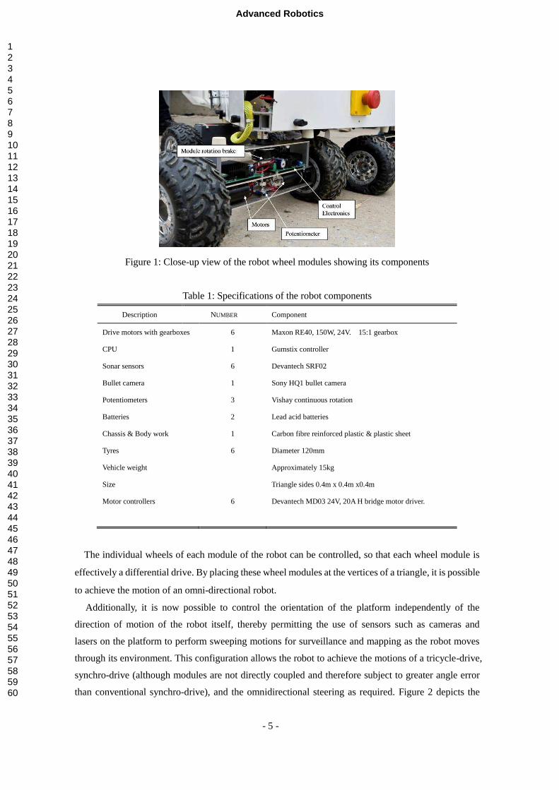
mobile-robot wheel configuration consisting of three wheel modules was developed. Figure 1

illustrates a corner of the vehicle with the wheel module covers removed.

On each module, the bottom section contains two motors with gearboxes mounted side by side. In

the centre of the module is the potentiometer that measures the module rotation with respect to the

vehicle orientation. The module upper row consist of a pair of motor power electronics and in the

centre a brake that allows the module angle with respect to the vehicle to be held constant (useful

when going over rough terrain). Table 1 has the specifications of the components used in the design

and construction of the robot.

123456789101112131415161718192021222324252627282930313233343536373839404142434445464748495051525354555657585960

- 5 -

Figure 1: Close-up view of the robot wheel modules showing its components

Table 1: Specifications of the robot components

Description NUMBER Component

Drive motors with gearboxes 6 Maxon RE40, 150W, 24V. 15:1 gearbox

CPU 1 Gumstix controller

Sonar sensors 6 Devantech SRF02

Bullet camera 1 Sony HQ1 bullet camera

Potentiometers 3 Vishay continuous rotation

Batteries 2 Lead acid batteries

Chassis & Body work 1 Carbon fibre reinforced plastic & plastic sheet

Tyres 6 Diameter 120mm

Vehicle weight Approximately 15kg

Size Triangle sides 0.4m x 0.4m x0.4m

Motor controllers 6 Devantech MD03 24V, 20A H bridge motor driver.

The individual wheels of each module of the robot can be controlled, so that each wheel module is

effectively a differential drive. By placing these wheel modules at the vertices of a triangle, it is possible

to achieve the motion of an omni-directional robot.

Additionally, it is now possible to control the orientation of the platform independently of the

direction of motion of the robot itself, thereby permitting the use of sensors such as cameras and

lasers on the platform to perform sweeping motions for surveillance and mapping as the robot moves

through its environment. This configuration allows the robot to achieve the motions of a tricycle-drive,

synchro-drive (although modules are not directly coupled and therefore subject to greater angle error

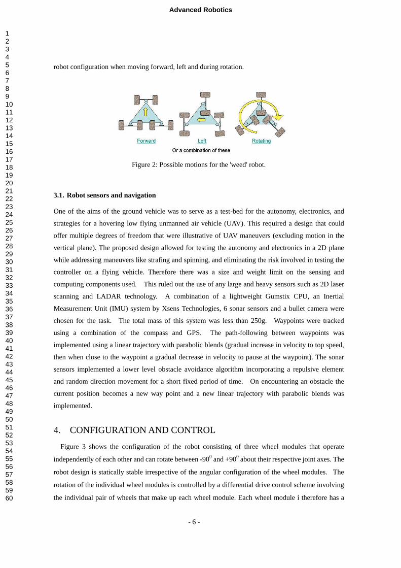
than conventional synchro-drive), and the omnidirectional steering as required. Figure 2 depicts the

Advanced Robotics

123456789101112131415161718192021222324252627282930313233343536373839404142434445464748495051525354555657585960

- 6 -

robot configuration when moving forward, left and during rotation.

Figure 2: Possible motions for the 'weed' robot.

3.1. Robot sensors and navigation

One of the aims of the ground vehicle was to serve as a test-bed for the autonomy, electronics, and

strategies for a hovering low flying unmanned air vehicle (UAV). This required a design that could

offer multiple degrees of freedom that were illustrative of UAV maneuvers (excluding motion in the

vertical plane). The proposed design allowed for testing the autonomy and electronics in a 2D plane

while addressing maneuvers like strafing and spinning, and eliminating the risk involved in testing the

controller on a flying vehicle. Therefore there was a size and weight limit on the sensing and

computing components used. This ruled out the use of any large and heavy sensors such as 2D laser

scanning and LADAR technology. A combination of a lightweight Gumstix CPU, an Inertial

Measurement Unit (IMU) system by Xsens Technologies, 6 sonar sensors and a bullet camera were

chosen for the task. The total mass of this system was less than 250g. Waypoints were tracked

using a combination of the compass and GPS. The path-following between waypoints was

implemented using a linear trajectory with parabolic blends (gradual increase in velocity to top speed,

then when close to the waypoint a gradual decrease in velocity to pause at the waypoint). The sonar

sensors implemented a lower level obstacle avoidance algorithm incorporating a repulsive element

and random direction movement for a short fixed period of time. On encountering an obstacle the

current position becomes a new way point and a new linear trajectory with parabolic blends was

implemented.

4. CONFIGURATION AND CONTROL

Figure 3 shows the configuration of the robot consisting of three wheel modules that operate

independently of each other and can rotate between -900 and +900 about their respective joint axes. The

robot design is statically stable irrespective of the angular configuration of the wheel modules. The

rotation of the individual wheel modules is controlled by a differential drive control scheme involving

the individual pair of wheels that make up each wheel module. Each wheel module i therefore has a

Advanced Robotics

123456789101112131415161718192021222324252627282930313233343536373839404142434445464748495051525354555657585960

- 7 -

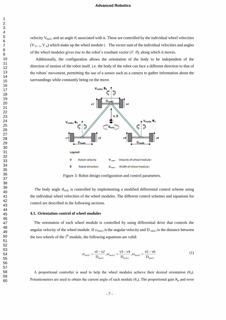
velocity Vmod i and an angle しi associated with it. These are controlled by the individual wheel velocities

(V 2i - 1, V 2i) which make up the wheel module i. The vector sum of the individual velocities and angles

of the wheel modules gives rise to the robot’s resultant vector (V, し), along which it moves.

Additionally, the configuration allows the orientation of the body to be independent of the

direction of motion of the robot itself. i.e. the body of the robot can face a different direction to that of

the robots’ movement, permitting the use of a sensor such as a camera to gather information about the

surroundings while constantly being on the move.

Figure 3: Robot design configuration and control parameters.

The body angle しbody is controlled by implementing a modified differential control scheme using

the individual wheel velocities of the wheel modules. The different control schemes and equations for

control are described in the following sections.

4.1. Orientation control of wheel modules

The orientation of each wheel module is controlled by using differential drive that controls the

angular velocity of the wheel module. If のmod i is the angular velocity and D mod i is the distance between

the two wheels of the ith module, the following equations are valid:

3mod3mod

2mod2mod

1mod1mod

65,

43,

21

D

vv

D

vv

D

vv

(1)

A proportional controller is used to help the wheel modules achieve their desired orientation (しd).

Potentiometers are used to obtain the current angle of each module (しa). The proportional gain Kp and error

Advanced Robotics

123456789101112131415161718192021222324252627282930313233343536373839404142434445464748495051525354555657585960

- 8 -

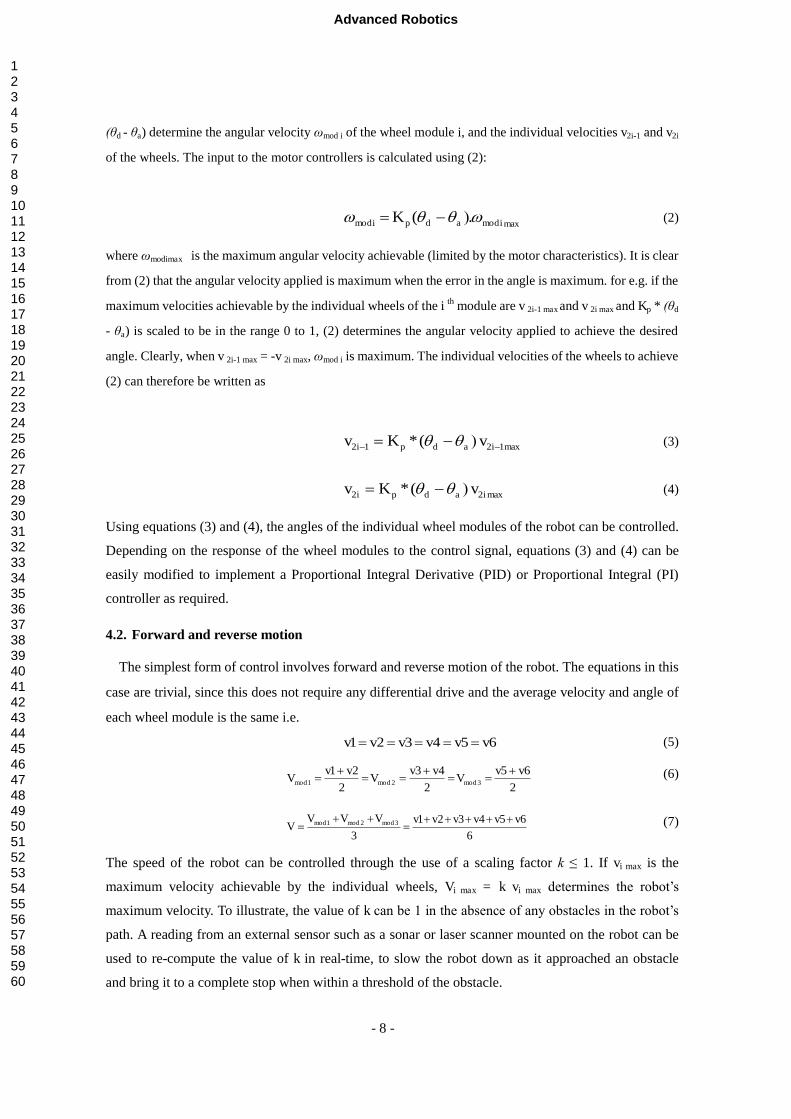
(しd - しa) determine the angular velocity のmod i of the wheel module i, and the individual velocities v2i-1 and v2i

of the wheels. The input to the motor controllers is calculated using (2):

maxmodpmod .(K iadi (2)

where のmodimax is the maximum angular velocity achievable (limited by the motor characteristics). It is clear

from (2) that the angular velocity applied is maximum when the error in the angle is maximum. for e.g. if the

maximum velocities achievable by the individual wheels of the i th module are v 2i-1 max and v 2i max and Kp * (しd

- しa) is scaled to be in the range 0 to 1, (2) determines the angular velocity applied to achieve the desired

angle. Clearly, when v 2i-1 max = -v 2i max, のmod i is maximum. The individual velocities of the wheels to achieve

(2) can therefore be written as

max12p12 ( * K iadi vv (3)

max2p2 ( * K iadi vv (4)

Using equations (3) and (4), the angles of the individual wheel modules of the robot can be controlled.

Depending on the response of the wheel modules to the control signal, equations (3) and (4) can be

easily modified to implement a Proportional Integral Derivative (PID) or Proportional Integral (PI)

controller as required.

4.2. Forward and reverse motion

The simplest form of control involves forward and reverse motion of the robot. The equations in this

case are trivial, since this does not require any differential drive and the average velocity and angle of

each wheel module is the same i.e.

654321 vvvvvv (5)

2

65

2

43

2

213mod2mod1mod

vvV

vvV

vvV

(6)

6

654321

33mod2mod1mod vvvvvvVVV

V

(7)

The speed of the robot can be controlled through the use of a scaling factor k ≤ 1. If vi max is the

maximum velocity achievable by the individual wheels, Vi max = k vi max determines the robot’s

maximum velocity. To illustrate, the value of k can be 1 in the absence of any obstacles in the robot’s

path. A reading from an external sensor such as a sonar or laser scanner mounted on the robot can be

used to re-compute the value of k in real-time, to slow the robot down as it approached an obstacle

and bring it to a complete stop when within a threshold of the obstacle.

Advanced Robotics

123456789101112131415161718192021222324252627282930313233343536373839404142434445464748495051525354555657585960

- 9 -

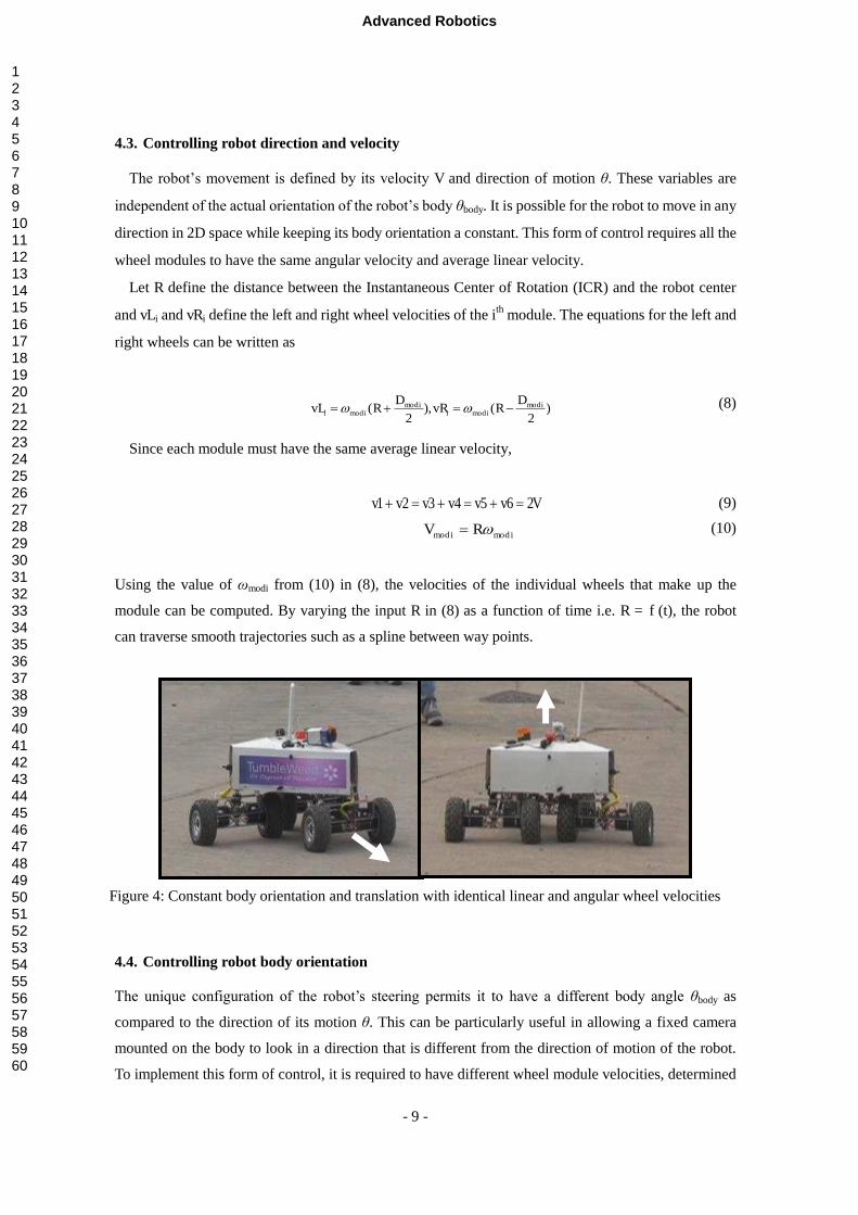
4.3. Controlling robot direction and velocity

The robot’s movement is defined by its velocity V and direction of motion し. These variables are

independent of the actual orientation of the robot’s body しbody. It is possible for the robot to move in any

direction in 2D space while keeping its body orientation a constant. This form of control requires all the

wheel modules to have the same angular velocity and average linear velocity.

Let R define the distance between the Instantaneous Center of Rotation (ICR) and the robot center

and vLi and vRi define the left and right wheel velocities of the ith module. The equations for the left and

right wheels can be written as

)2

(),2

( modmod

modmod

iii

iii

DRvR

DRvL (8)

Since each module must have the same average linear velocity,

Vvvvvvv 2654321 (9)

ii RV modmod (10)

Using the value of のmodi from (10) in (8), the velocities of the individual wheels that make up the

module can be computed. By varying the input R in (8) as a function of time i.e. R = f (t), the robot

can traverse smooth trajectories such as a spline between way points.

4.4. Controlling robot body orientation

The unique configuration of the robot’s steering permits it to have a different body angle しbody as

compared to the direction of its motion し. This can be particularly useful in allowing a fixed camera

mounted on the body to look in a direction that is different from the direction of motion of the robot.

To implement this form of control, it is required to have different wheel module velocities, determined

Figure 4: Constant body orientation and translation with identical linear and angular wheel velocities

Advanced Robotics

123456789101112131415161718192021222324252627282930313233343536373839404142434445464748495051525354555657585960

- 10 -

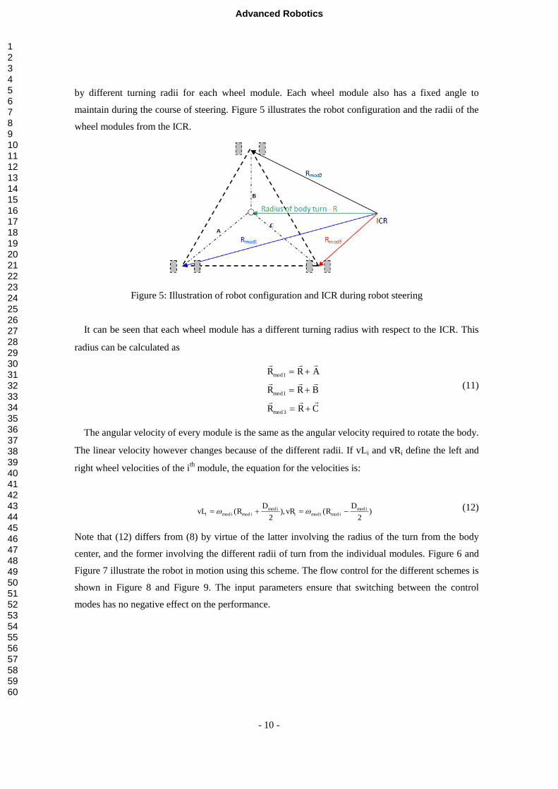
by different turning radii for each wheel module. Each wheel module also has a fixed angle to

maintain during the course of steering. Figure 5 illustrates the robot configuration and the radii of the

wheel modules from the ICR.

Figure 5: Illustration of robot configuration and ICR during robot steering

It can be seen that each wheel module has a different turning radius with respect to the ICR. This

radius can be calculated as

CRR

BRR

ARR

3mod

1mod

1mod

(11)

The angular velocity of every module is the same as the angular velocity required to rotate the body.

The linear velocity however changes because of the different radii. If vLi and vRi define the left and

right wheel velocities of the ith module, the equation for the velocities is:

)2

(),2

( modmodmod

modmodmod

iiii

iiii

DRvR

DRvL (12)

Note that (12) differs from (8) by virtue of the latter involving the radius of the turn from the body

center, and the former involving the different radii of turn from the individual modules. Figure 6 and

Figure 7 illustrate the robot in motion using this scheme. The flow control for the different schemes is

shown in Figure 8 and Figure 9. The input parameters ensure that switching between the control

modes has no negative effect on the performance.

Advanced Robotics

123456789101112131415161718192021222324252627282930313233343536373839404142434445464748495051525354555657585960

- 11 -

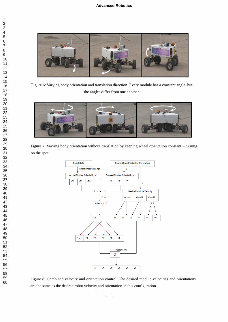
Figure 8: Combined velocity and orientation control. The desired module velocities and orientations

are the same as the desired robot velocity and orientation in this configuration.

Figure 6: Varying body orientation and translation direction. Every module has a constant angle, but

the angles differ from one another.

Figure 7: Varying body orientation without translation by keeping wheel orientation constant – turning

on the spot.

Advanced Robotics

123456789101112131415161718192021222324252627282930313233343536373839404142434445464748495051525354555657585960

- 12 -

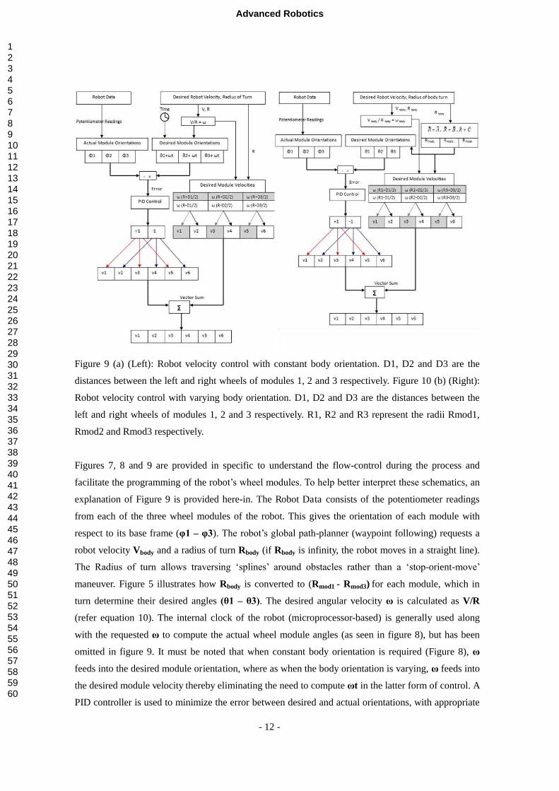
Figure 9 (a) (Left): Robot velocity control with constant body orientation. D1, D2 and D3 are the

distances between the left and right wheels of modules 1, 2 and 3 respectively. Figure 10 (b) (Right):

Robot velocity control with varying body orientation. D1, D2 and D3 are the distances between the

left and right wheels of modules 1, 2 and 3 respectively. R1, R2 and R3 represent the radii Rmod1,

Rmod2 and Rmod3 respectively.

Figures 7, 8 and 9 are provided in specific to understand the flow-control during the process and

facilitate the programming of the robot’s wheel modules. To help better interpret these schematics, an

explanation of Figure 9 is provided here-in. The Robot Data consists of the potentiometer readings

from each of the three wheel modules of the robot. This gives the orientation of each module with

respect to its base frame (l1 – l3). The robot’s global path-planner (waypoint following) requests a

robot velocity Vbody and a radius of turn Rbody (if Rbody is infinity, the robot moves in a straight line).

The Radius of turn allows traversing ‘splines’ around obstacles rather than a ‘stop-orient-move’

maneuver. Figure 5 illustrates how Rbody is converted to (Rmod1 - Rmod3) for each module, which in

turn determine their desired angles (し1 – し3). The desired angular velocity の is calculated as V/R

(refer equation 10). The internal clock of the robot (microprocessor-based) is generally used along

with the requested の to compute the actual wheel module angles (as seen in figure 8), but has been

omitted in figure 9. It must be noted that when constant body orientation is required (Figure 8), の

feeds into the desired module orientation, where as when the body orientation is varying, の feeds into

the desired module velocity thereby eliminating the need to compute のt in the latter form of control. A

PID controller is used to minimize the error between desired and actual orientations, with appropriate

Advanced Robotics

123456789101112131415161718192021222324252627282930313233343536373839404142434445464748495051525354555657585960

- 13 -

sign conventions (+/-) used to compute the velocity for each individual wheel (6 wheels, 3 modules).

The desired module velocities are calculated from which individual wheel velocities (v1 – v6) can be

computed (equation (12)). A vector sum of these velocities, with the velocities from the PID control is

used to determine the final velocities for each of the wheels of the three modules to perform the

requested robot motion. As mentioned previously, this scheme can be extended to thruster / fans for

underwater robots and air vehicles. A video demonstration of the robot using these algorithms for

locomotion can be found here [28].

5. SIMULATED TRAJECTORIES OF COMPLEX MOTION

The equations of motion developed in section 4 (equations 1 – 12) are used to simulate robot motion

for different movement trajectories.

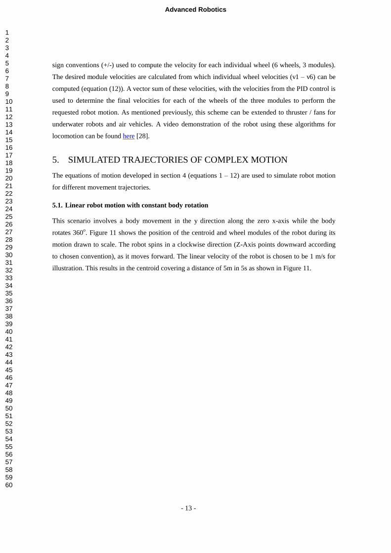
5.1. Linear robot motion with constant body rotation

This scenario involves a body movement in the y direction along the zero x-axis while the body

rotates 360o. Figure 11 shows the position of the centroid and wheel modules of the robot during its

motion drawn to scale. The robot spins in a clockwise direction (Z-Axis points downward according

to chosen convention), as it moves forward. The linear velocity of the robot is chosen to be 1 m/s for

illustration. This results in the centroid covering a distance of 5m in 5s as shown in Figure 11.

Advanced Robotics

123456789101112131415161718192021222324252627282930313233343536373839404142434445464748495051525354555657585960

- 14 -

Figure 11: Linear motion with constant body rotation.

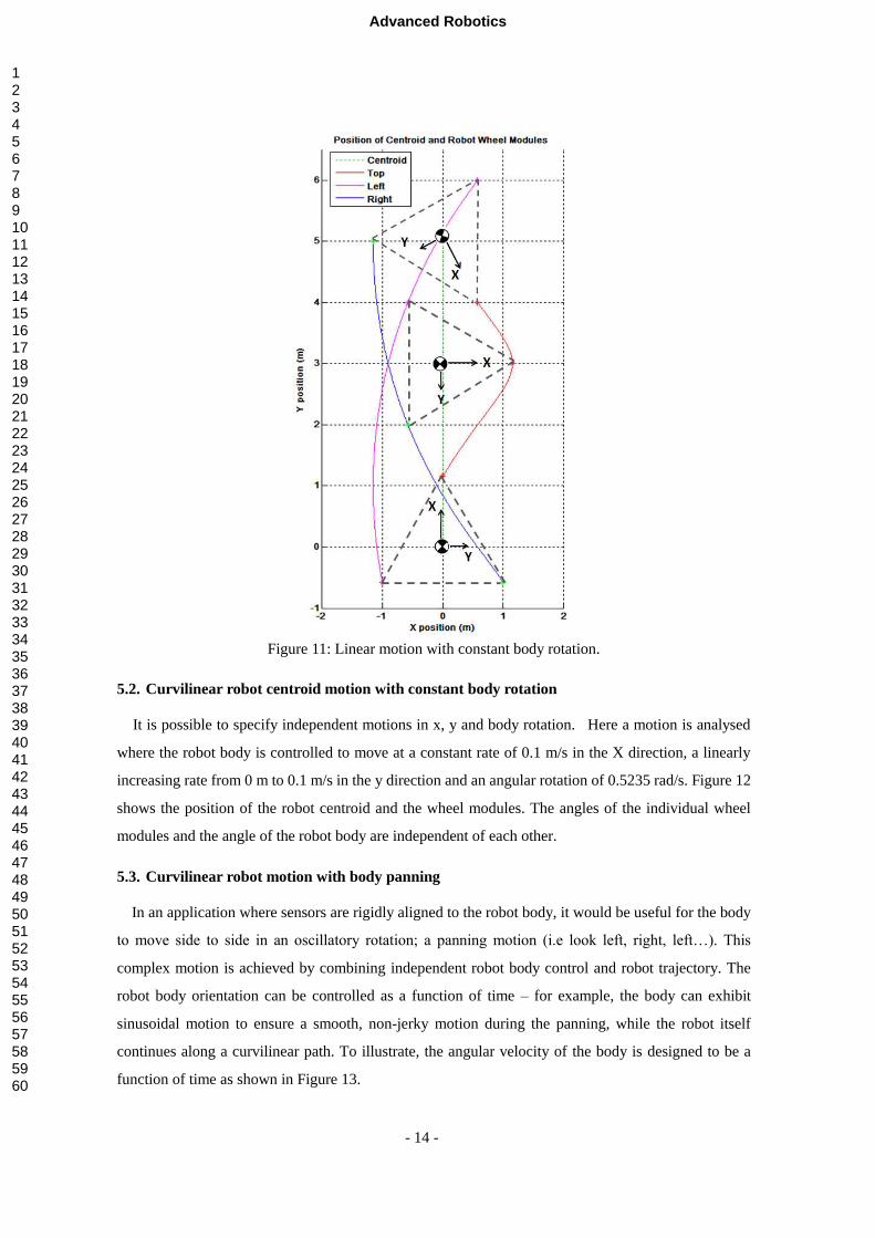
5.2. Curvilinear robot centroid motion with constant body rotation

It is possible to specify independent motions in x, y and body rotation. Here a motion is analysed

where the robot body is controlled to move at a constant rate of 0.1 m/s in the X direction, a linearly

increasing rate from 0 m to 0.1 m/s in the y direction and an angular rotation of 0.5235 rad/s. Figure 12

shows the position of the robot centroid and the wheel modules. The angles of the individual wheel

modules and the angle of the robot body are independent of each other.

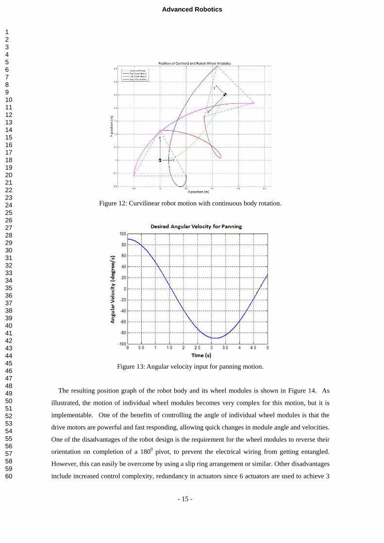
5.3. Curvilinear robot motion with body panning

In an application where sensors are rigidly aligned to the robot body, it would be useful for the body

to move side to side in an oscillatory rotation; a panning motion (i.e look left, right, left…). This

complex motion is achieved by combining independent robot body control and robot trajectory. The

robot body orientation can be controlled as a function of time – for example, the body can exhibit

sinusoidal motion to ensure a smooth, non-jerky motion during the panning, while the robot itself

continues along a curvilinear path. To illustrate, the angular velocity of the body is designed to be a

function of time as shown in Figure 13.

Advanced Robotics

123456789101112131415161718192021222324252627282930313233343536373839404142434445464748495051525354555657585960

- 15 -

Figure 12: Curvilinear robot motion with continuous body rotation.

Figure 13: Angular velocity input for panning motion.

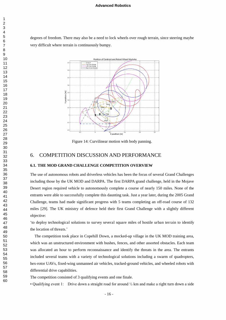
The resulting position graph of the robot body and its wheel modules is shown in Figure 14. As

illustrated, the motion of individual wheel modules becomes very complex for this motion, but it is

implementable. One of the benefits of controlling the angle of individual wheel modules is that the

drive motors are powerful and fast responding, allowing quick changes in module angle and velocities.

One of the disadvantages of the robot design is the requirement for the wheel modules to reverse their

orientation on completion of a 1800 pivot, to prevent the electrical wiring from getting entangled.

However, this can easily be overcome by using a slip ring arrangement or similar. Other disadvantages

include increased control complexity, redundancy in actuators since 6 actuators are used to achieve 3

Advanced Robotics

123456789101112131415161718192021222324252627282930313233343536373839404142434445464748495051525354555657585960

- 16 -

degrees of freedom. There may also be a need to lock wheels over rough terrain, since steering maybe

very difficult where terrain is continuously bumpy.

Figure 14: Curvilinear motion with body panning.

6. COMPETITION DISCUSSION AND PERFORMANCE

6.1. THE MOD GRAND CHALLENGE COMPETITION OVERVIEW

The use of autonomous robots and driverless vehicles has been the focus of several Grand Challenges

including those by the UK MOD and DARPA. The first DARPA grand challenge, held in the Mojave

Desert region required vehicle to autonomously complete a course of nearly 150 miles. None of the

entrants were able to successfully complete this daunting task. Just a year later, during the 2005 Grand

Challenge, teams had made significant progress with 5 teams completing an off-road course of 132

miles [29]. The UK ministry of defence held their first Grand Challenge with a slightly different

objective:

‘to deploy technological solutions to survey several square miles of hostile urban terrain to identify

the location of threats.’

The competition took place in Copehill Down, a mocked-up village in the UK MOD training area,

which was an unstructured environment with bushes, fences, and other assorted obstacles. Each team

was allocated an hour to perform reconnaissance and identify the threats in the area. The entrants

included several teams with a variety of technological solutions including a swarm of quadropters,

hex-rotor UAVs, fixed-wing unmanned air vehicles, tracked-ground vehicles, and wheeled robots with

differential drive capabilities.

The competition consisted of 3 qualifying events and one finale.

• Qualifying event 1: Drive down a straight road for around ½ km and make a right turn down a side

Advanced Robotics

123456789101112131415161718192021222324252627282930313233343536373839404142434445464748495051525354555657585960

- 17 -

road for another 40m.

• Qualifying event 2: Drive into an area ½ km x ½ km and automatically identify the location of a

truck with a gun on the back

• Qualifying event 3: Survey an area approximately 1km x 1km and identify as many threats as

possible

• Finale: Survey an area approximately 2km x 2km and identify as many threats and improvised

explosive devices as possible.

A three-module differential-drive robot called ‘weed’ was designed and constructed as an entrant into

this competition. The following sections highlight the related literature in the area, followed by

detailing the robot’s design, construction, configuration and control. Finally, results of field

deployment are presented.

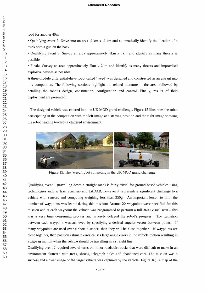
The designed vehicle was entered into the UK MOD grand challenge. Figure 15 illustrates the robot

participating in the competition with the left image at a starting position and the right image showing

the robot heading towards a cluttered environment.

Figure 15: The ‘weed’ robot competing in the UK MOD grand challenge.

Qualifying event 1 (travelling down a straight road) is fairly trivial for ground based vehicles using

technologies such as laser scanners and LADAR, however it represents a significant challenge to a

vehicle with sensors and computing weighing less than 250g. An important lesson to limit the

number of waypoints was learnt during this mission: Around 20 waypoints were specified for this

mission and at each waypoint the vehicle was programmed to perform a full 3600 visual scan – this

was a very time consuming process and severely delayed the robot’s progress. The transition

between each waypoint was achieved by specifying a desired angular vector between points. If

many waypoints are used over a short distance, then they will be close together. If waypoints are

close together, then position estimate error causes large angle errors in the vehicle motion resulting in

a zig-zag motion when the vehicle should be travelling in a straight line.

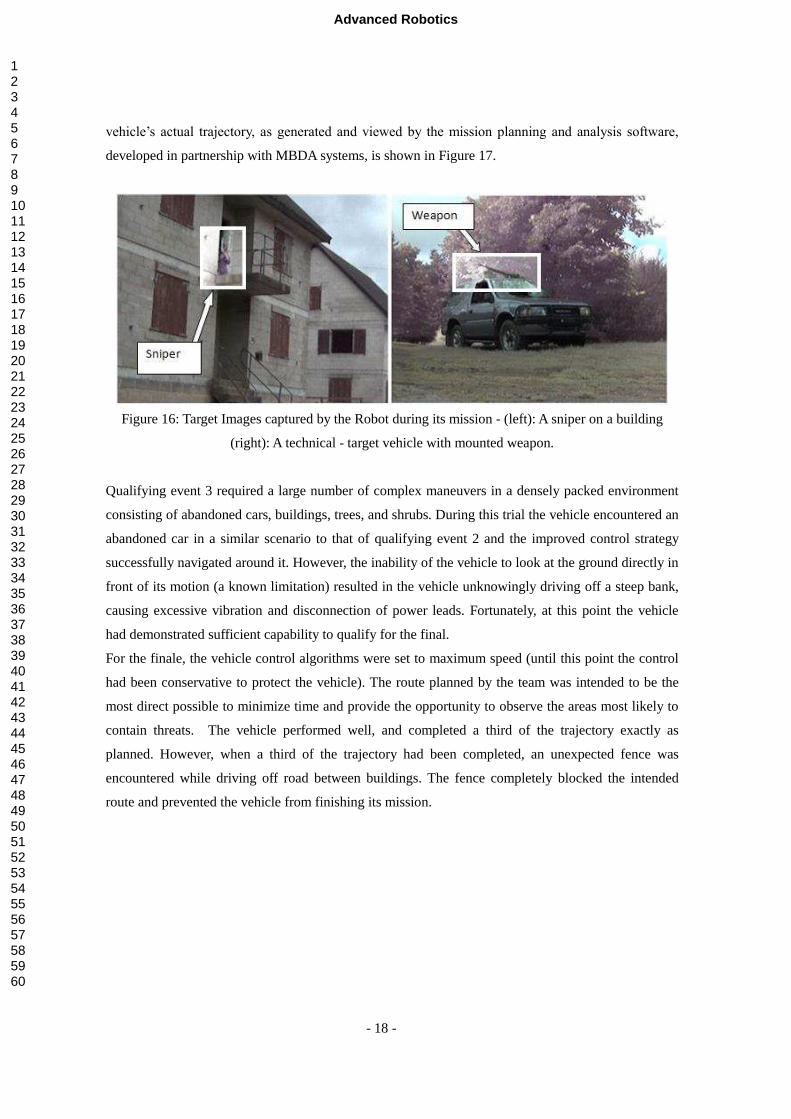
Qualifying event 2 required several turns on minor roads/dirt tracks that were difficult to make in an

environment cluttered with trees, shrubs, telegraph poles and abandoned cars. The mission was a

success and a clear image of the target vehicle was captured by the vehicle (Figure 16). A map of the

Advanced Robotics

123456789101112131415161718192021222324252627282930313233343536373839404142434445464748495051525354555657585960

- 18 -

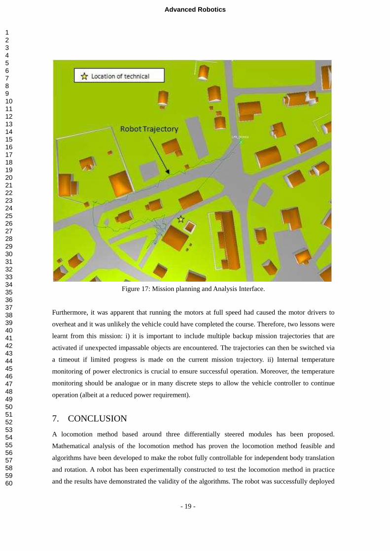
vehicle’s actual trajectory, as generated and viewed by the mission planning and analysis software,

developed in partnership with MBDA systems, is shown in Figure 17.

Figure 16: Target Images captured by the Robot during its mission - (left): A sniper on a building

(right): A technical - target vehicle with mounted weapon.

Qualifying event 3 required a large number of complex maneuvers in a densely packed environment

consisting of abandoned cars, buildings, trees, and shrubs. During this trial the vehicle encountered an

abandoned car in a similar scenario to that of qualifying event 2 and the improved control strategy

successfully navigated around it. However, the inability of the vehicle to look at the ground directly in

front of its motion (a known limitation) resulted in the vehicle unknowingly driving off a steep bank,

causing excessive vibration and disconnection of power leads. Fortunately, at this point the vehicle

had demonstrated sufficient capability to qualify for the final.

For the finale, the vehicle control algorithms were set to maximum speed (until this point the control

had been conservative to protect the vehicle). The route planned by the team was intended to be the

most direct possible to minimize time and provide the opportunity to observe the areas most likely to

contain threats. The vehicle performed well, and completed a third of the trajectory exactly as

planned. However, when a third of the trajectory had been completed, an unexpected fence was

encountered while driving off road between buildings. The fence completely blocked the intended

route and prevented the vehicle from finishing its mission.

Advanced Robotics

123456789101112131415161718192021222324252627282930313233343536373839404142434445464748495051525354555657585960

- 19 -

Figure 17: Mission planning and Analysis Interface.

Furthermore, it was apparent that running the motors at full speed had caused the motor drivers to

overheat and it was unlikely the vehicle could have completed the course. Therefore, two lessons were

learnt from this mission: i) it is important to include multiple backup mission trajectories that are

activated if unexpected impassable objects are encountered. The trajectories can then be switched via

a timeout if limited progress is made on the current mission trajectory. ii) Internal temperature

monitoring of power electronics is crucial to ensure successful operation. Moreover, the temperature

monitoring should be analogue or in many discrete steps to allow the vehicle controller to continue

operation (albeit at a reduced power requirement).

7. CONCLUSION

A locomotion method based around three differentially steered modules has been proposed.

Mathematical analysis of the locomotion method has proven the locomotion method feasible and

algorithms have been developed to make the robot fully controllable for independent body translation

and rotation. A robot has been experimentally constructed to test the locomotion method in practice

and the results have demonstrated the validity of the algorithms. The robot was successfully deployed

Advanced Robotics

123456789101112131415161718192021222324252627282930313233343536373839404142434445464748495051525354555657585960

- 20 -

in the UK MOD grand challenge. The design and control strategies permit mounting sensors for

surveillance without the need for turret-based sensors which require additional sensors to localize

them and also minimizing the number of moving-parts on a robot. Future work involves modifying

the chassis to include active suspension mechanisms for mobility on uneven terrain.

ACKNOWLEDGEMENTS

The authors gratefully acknowledge the support of BAE systems and MBDA. They would also like

to thank the organizers and event managers of the Grand Challenge for making the event possible.

REFERENCES

[1] G. Dissanayake, P. Newman, H.F. Durrant-Whyte, S. Clark, and M. Csobra, A solution to the

simultaneous localisation and mapping (SLAM) problem, IEEE Transactions on Robotics and

Automation, vol. 17, no. 3, pp. 229–241, 2001.

[2] C.C. Wang, C. Thorpe, and S. Thrun, On-line simultaneous localisation and mapping with

detection and tracking of moving objects, in Proc. IEEE Int. Conf. Robotics and Automation, 2003,

pp. 2918–2924.

[3] A.J. Davison, Y.G. Cid, and N. Kita, Real-time 3D SLAM with wide-angle vision, in Proc.

IFAC/EURON Symp. Intell. Auton. Vehicles, 2004.

[4] E. U. Acar, Y. Zhang, H. Choset, M. Schervish, A. G. Costa, R. Melamud, D. C. Lean, and A.

Graveline, Path Planning for Robotic Demining and Development of a Test Platform, In

Proceedings of the 3rd International Conference on Field and Service Robotics (FSR), pp. 161-168,

2001.

[5] Maddocks, J. H., & Alexander, J. C. (1987). On the Kinematics and Control of Wheeled Mobile

Robots: Maryland University College Park Systems Research Center.

[6] Everett, H. R. (1995). Sensors for mobile robots: theory and application: AK Peters, Ltd.

[7] Podnar, G., Dowling, D., Blackwell, M., & Carnegie-Mellon Univ Pittsburgh Pa Robotics, I.

(1984). A functional vehicle for autonomous mobile robot research: Citeseer.

[8] Crowley, J. L., & Reignier, P. (1992). Asynchronous control of rotation and translation for a robot

vehicle. Robotics and Autonomous Systems, 10(4), 243-251.

[9] Meng, Q., & Bischoff, R. (2005). Odometry based pose determination and errors measurement for

a mobile robot with two steerable drive wheels. Journal of Intelligent and Robotic Systems, 41(4),

263-282.

[10] Byrne, R. H., Abdallah, C. T., & Dorato, P. (2002). Experimental results in robust lateral control of

highway vehicles. Control Systems Magazine, IEEE, 18(2), 70-76.

123456789101112131415161718192021222324252627282930313233343536373839404142434445464748495051525354555657585960

Advanced Robotics

- 21 -

[11] Borenstein, J., Everett, H. R., & Feng, L. (1996). Where am I? Sensors and methods for mobile

robot positioning. Technical report, University of Michigan, 119, 120.

[12] Borenstein, J. (1995). Control and kinematic design of multi-degree-of-freedom mobile robots with

compliant linkage. IEEE Transactions on Robotics and Automation, 11(1), 21-35.

[13] Abou-Samah, M., & Krovi, V. (2001). Cooperative Frameworks for Multiple Mobile Robots. In:

CCTOMM Symposium on Mechanisms, Machines and Mechatronics.

[14] Pin, F. G., Beckerman, M., Spelt, P. F., Robinson, J. T., & Weisbin, C. R. (1989). Autonomous

mobile robot research using the HERMIES-III robot: Oak Ridge National Lab., TN (USA).

[15] Reister, D. B. (1992). A new wheel control system for the omnidirectional HERMIES-III robot.

Robotica, 10(04), 351-360.

[16] Fisher, D., Holland, J. M., & Kennedy, K. F. (1994). K3A Marks Third Generation SynchroDrive.

Proc. of ANS Robotics and Remote Systems, ANS Annual Meeting, New Orleans, LA, June 19-23.

[17] Carlisle, B. (1983). An omni-directional mobile robot. Developments in Robotics, 79–87.

[18] Yu, H., Dubowsky, S., and Skwersky, A., Omni-directional Mobility Using Active Split Offset

Castors. Proc of the 26th ASME Biennial Mechanisms and Robotics Conf, Sep 2000.

[19] Davis, J. J., Doebbler, J., Daugherty, K., Junkins, J. L., and Valasek, J., Aerospace Vehicle Motion

Emulation Using Omni-Directional Mobile Platform, presented at the AIAA Guidance,

Navigation, and Control Conference, Hilton Head, South Carolina, August 2007.

[20] Udengaard, M. and Iagnemma, K., 2008: Design of an Omnidirectional Mobile for Rough Terrain,

Proc of IEEE Intl Conf on Robotics and Automation, 1666-1671.

[21] Ishigami, G., Pineda, E., Overholt, J., Hudas, G., & Iagnemma, K. (2011, September). Performance

analysis and odometry improvement of an omnidirectional mobile robot for outdoor terrain. In

Intelligent Robots and Systems (IROS), 2011 IEEE/RSJ International Conference on (pp.

4091-4096). IEEE.

[22] Tadakuma, K., Tadakuma, R., & Berengueres, J. (2008). Tetrahedral mobile robot with spherical

omnidirectional wheel. Journal of Robotics and Mechatronics, 20(1), 125.

[23] Tadakuma, K., Tadakuma, R., & Berengeres, J. (2007, October). Development of holonomic

omnidirectional Vehicle with “Omni-Ball”: spherical wheels. InIntelligent Robots and Systems,

2007. IROS 2007. IEEE/RSJ International Conference on (pp. 33-39). IEE

[24] Wilcox, B. H. (2009, March). ATHLETE: A cargo and habitat transporter for the moon.

In Aerospace conference, 2009 IEEE (pp. 1-7). IEEE.

[25] Salih, J. E. M., Rizon, M., Yaacob, S., Adom, A. H., & Mamat, M. R. (2006). Designing

omni-directional mobile robot with mecanum wheel. American Journal of Applied Sciences, 3(5),

1831-1835.

[26] Tlale, N., & de Villiers, M. (2008, December). Kinematics and dynamics modelling of a mecanum

wheeled mobile platform. In Mechatronics and Machine Vision in Practice, 2008. M2VIP 2008.

15th International Conference on (pp. 657-662). IEEE.

Advanced Robotics

123456789101112131415161718192021222324252627282930313233343536373839404142434445464748495051525354555657585960

- 22 -

[27] Ye, C., & Ma, S. (2009, August). Development of an omnidirectional mobile platform.

In Mechatronics and Automation, 2009. ICMA 2009. International Conference on (pp.

1111-1115). IEEE.

[28] Video demonstration of the robot maneuvers [http://youtu.be/KW-Ne540OQA]

[29] Thrun, S. (2006). Winning the darpa grand challenge. Machine Learning: ECML 2006, 4-4.

123456789101112131415161718192021222324252627282930313233343536373839404142434445464748495051525354555657585960

Advanced Robotics