Design and Implementation of an EKF based SLAM algorithm on amobile robot

Thesis submitted in partial fulfillmentof the requirements for the degree of

MS by Researchin

Computer Science and Engineering

by

Gururaj Kosuru200707006

gururaj@research.iiit.ac.in

Robotics Research LabInternational Institute of Information Technology

Hyderabad - 500 032, IndiaOctober 2011

Copyright c© Gururaj Kosuru, 2011

All Rights Reserved

International Institute of Information TechnologyHyderabad, India

CERTIFICATE

It is certified that the work contained in this thesis, titled “Design and Implementation of an EKF basedSLAM algorithm on a mobile robot” by Gururaj Kosuru, has been carried out under my supervision andis not submitted elsewhere for a degree.

Date Adviser: Dr. K. Madhava Krishna

To my parents

Sheela and Madhav

Acknowledgments

I am very grateful to my guide, Dr. Madhava Krishna for his support and confidence in me. I willalways be indebted to him for his invaluable guidance during difficult times. His friendly and informalmethods of interaction have helped instill confidence in me and improve my performance.

I would particularly like to acknowledge the role of my mother who has always been there for me. Iam also thankful to my friends who have always helped in improving my understanding of everythingunder the sun and have been there for me.

v

Abstract

The importance of environment modelling as a prerequisite for the navigation of mobile robots can-not be understated. It is essential for a mobile robot to have the ability to autonomously build a modelof the environment, as human intervention is not practical in all circumstances. The unavailability ofenvironment modelling algorithms until recently, has hampered the feasibility of the envisaged vision ofmobile robotics. A robot has to address both the mapping and the localization problems in order to au-tonomously solve the map learning problem. Due to the coupling between these two tasks, autonomousmap learning has been a challenging problem. This thesis is primarily focused on the implementationof an environment modelling technique based on the Extended Kalman Filter(EKF). The mapping andlocalization problem, called Simultaneous Localization And Mapping(SLAM) is defined as the processof concurrently building a map of the environment while using this map to obtain improved estimates ofthe robot location. The SLAM algorithm begins with the mobile robot in an unknown location, with noa priori knowledge of the map. The robot then uses a sensor to model the visible environment and simul-taneously computes an estimate of its own position. Continuing in motion, the mobile robot eventuallybuilds a model of the environment which is useful for navigation.

In spite of the ample literature available on SLAM, there is hardly any literature on the developmentof a real SLAM system. A majority of the work in this thesis is attributed to filling the gap betweentheory and implementation by the identification and diagnosis of the issues faced during implementation.The work in this thesis can be divided into two sections: contributions in the implementation front andthose in the theoretical front. The implementation part deals with the system specific customizationof the algorithm, a novel calibration method for the sensor with respect to the robot, extraction andparametrization of features, provision for manual exploration during map building among other issues.This part of the thesis concludes with successful demonstrations of robust EKF-SLAM implementationon the Pioneer P3-Dx mobile robot using a SICK LMS200 range scanning sensor. The theoreticalwork in this thesis deals with better map building by novel parametrizations of features to keep errorestimates low, representative features for better association and trajectory estimation from the onlineSLAM problem.

vi

Contents

Chapter Page

Acknowledgements . . . . . . . . . . . . . . . . . . . . . . . . . . . . . . . . . . . . . . v

Abstract . . . . . . . . . . . . . . . . . . . . . . . . . . . . . . . . . . . . . . . . . . . . vi

1 Introduction . . . . . . . . . . . . . . . . . . . . . . . . . . . . . . . . . . . . . . . . . . 11.1 Background and Motivation . . . . . . . . . . . . . . . . . . . . . . . . . . . . . . . 21.2 Related Work . . . . . . . . . . . . . . . . . . . . . . . . . . . . . . . . . . . . . . . 51.3 Contributions . . . . . . . . . . . . . . . . . . . . . . . . . . . . . . . . . . . . . . . 61.4 Organization of this thesis . . . . . . . . . . . . . . . . . . . . . . . . . . . . . . . . 7

2 Simultaneous Localisation And Mapping . . . . . . . . . . . . . . . . . . . . . . . . . . . 92.1 Introduction . . . . . . . . . . . . . . . . . . . . . . . . . . . . . . . . . . . . . . . . 102.2 Estimation of a Dynamic System . . . . . . . . . . . . . . . . . . . . . . . . . . . . . 10

2.2.1 The Markov Property . . . . . . . . . . . . . . . . . . . . . . . . . . . . . . . 112.2.2 Mean and Variance Propagation . . . . . . . . . . . . . . . . . . . . . . . . . 122.2.3 The Kalman Filter . . . . . . . . . . . . . . . . . . . . . . . . . . . . . . . . 13

2.3 The EKF-SLAM Model . . . . . . . . . . . . . . . . . . . . . . . . . . . . . . . . . 162.3.1 The State Vector . . . . . . . . . . . . . . . . . . . . . . . . . . . . . . . . . 162.3.2 Vehicle Motion Model . . . . . . . . . . . . . . . . . . . . . . . . . . . . . . 172.3.3 Feature Model . . . . . . . . . . . . . . . . . . . . . . . . . . . . . . . . . . 182.3.4 Sensor Measurement Model . . . . . . . . . . . . . . . . . . . . . . . . . . . 182.3.5 Brief Description . . . . . . . . . . . . . . . . . . . . . . . . . . . . . . . . . 192.3.6 The Process Evolution . . . . . . . . . . . . . . . . . . . . . . . . . . . . . . 19

2.4 The EKF-SLAM Algorithm . . . . . . . . . . . . . . . . . . . . . . . . . . . . . . . 212.4.1 Prediction Stage . . . . . . . . . . . . . . . . . . . . . . . . . . . . . . . . . 212.4.2 Observation Stage . . . . . . . . . . . . . . . . . . . . . . . . . . . . . . . . 222.4.3 Update Stage . . . . . . . . . . . . . . . . . . . . . . . . . . . . . . . . . . . 222.4.4 Augment Stage . . . . . . . . . . . . . . . . . . . . . . . . . . . . . . . . . . 23

2.5 Summary . . . . . . . . . . . . . . . . . . . . . . . . . . . . . . . . . . . . . . . . . 26

3 System Development . . . . . . . . . . . . . . . . . . . . . . . . . . . . . . . . . . . . . . 273.1 The Test-bed . . . . . . . . . . . . . . . . . . . . . . . . . . . . . . . . . . . . . . . 273.2 Parametrization . . . . . . . . . . . . . . . . . . . . . . . . . . . . . . . . . . . . . . 28

3.2.1 Motion Model . . . . . . . . . . . . . . . . . . . . . . . . . . . . . . . . . . 293.2.2 Sensor Model . . . . . . . . . . . . . . . . . . . . . . . . . . . . . . . . . . . 31

vii

viii CONTENTS

3.3 Simulation . . . . . . . . . . . . . . . . . . . . . . . . . . . . . . . . . . . . . . . . . 313.3.1 Scalar Implementation . . . . . . . . . . . . . . . . . . . . . . . . . . . . . . 313.3.2 EKF-SLAM Simulation . . . . . . . . . . . . . . . . . . . . . . . . . . . . . 34

3.4 Real System Implementation . . . . . . . . . . . . . . . . . . . . . . . . . . . . . . . 353.4.1 Calibration . . . . . . . . . . . . . . . . . . . . . . . . . . . . . . . . . . . . 35

3.4.1.1 Pitch and Roll Error Calibration . . . . . . . . . . . . . . . . . . . . 373.4.1.2 Yaw and Translation Error Calibration . . . . . . . . . . . . . . . . 38

3.4.2 Independent Frame of reference . . . . . . . . . . . . . . . . . . . . . . . . . 413.4.3 Exploration . . . . . . . . . . . . . . . . . . . . . . . . . . . . . . . . . . . . 413.4.4 Online and Offline Versions . . . . . . . . . . . . . . . . . . . . . . . . . . . 41

3.4.4.1 Online SLAM . . . . . . . . . . . . . . . . . . . . . . . . . . . . . 423.4.4.2 Offline SLAM . . . . . . . . . . . . . . . . . . . . . . . . . . . . . 42

3.4.5 Complete Metric Map Building . . . . . . . . . . . . . . . . . . . . . . . . . 433.4.5.1 Smoothing . . . . . . . . . . . . . . . . . . . . . . . . . . . . . . . 44

3.5 Summary . . . . . . . . . . . . . . . . . . . . . . . . . . . . . . . . . . . . . . . . . 45

4 Features . . . . . . . . . . . . . . . . . . . . . . . . . . . . . . . . . . . . . . . . . . . . 474.1 Types of Features . . . . . . . . . . . . . . . . . . . . . . . . . . . . . . . . . . . . . 474.2 Point Features . . . . . . . . . . . . . . . . . . . . . . . . . . . . . . . . . . . . . . . 48

4.2.1 Parametrization of Point Features . . . . . . . . . . . . . . . . . . . . . . . . 484.2.2 Point Feature Extraction . . . . . . . . . . . . . . . . . . . . . . . . . . . . . 49

4.2.2.1 Data Clustering . . . . . . . . . . . . . . . . . . . . . . . . . . . . 494.2.2.2 Split-and-Merge Line Division . . . . . . . . . . . . . . . . . . . . 49

4.2.3 Point Feature Association . . . . . . . . . . . . . . . . . . . . . . . . . . . . 504.2.4 Point Feature Augmentation . . . . . . . . . . . . . . . . . . . . . . . . . . . 51

4.3 Line based features . . . . . . . . . . . . . . . . . . . . . . . . . . . . . . . . . . . . 534.3.1 Parametrization of Line based features . . . . . . . . . . . . . . . . . . . . . . 544.3.2 Line Feature Extraction . . . . . . . . . . . . . . . . . . . . . . . . . . . . . . 554.3.3 Line Feature Association . . . . . . . . . . . . . . . . . . . . . . . . . . . . . 554.3.4 Line Feature Augmentation . . . . . . . . . . . . . . . . . . . . . . . . . . . 574.3.5 Results . . . . . . . . . . . . . . . . . . . . . . . . . . . . . . . . . . . . . . 58

4.4 MECP Features . . . . . . . . . . . . . . . . . . . . . . . . . . . . . . . . . . . . . . 614.4.1 Parametrization of MECP Features . . . . . . . . . . . . . . . . . . . . . . . 614.4.2 MECP Feature Extraction . . . . . . . . . . . . . . . . . . . . . . . . . . . . 614.4.3 MECP Feature Association . . . . . . . . . . . . . . . . . . . . . . . . . . . . 634.4.4 MECP Feature Augmentation . . . . . . . . . . . . . . . . . . . . . . . . . . 644.4.5 Results . . . . . . . . . . . . . . . . . . . . . . . . . . . . . . . . . . . . . . 64

4.5 Summary . . . . . . . . . . . . . . . . . . . . . . . . . . . . . . . . . . . . . . . . . 68

5 Results . . . . . . . . . . . . . . . . . . . . . . . . . . . . . . . . . . . . . . . . . . . . . 695.1 Experiments in modelled environments . . . . . . . . . . . . . . . . . . . . . . . . . 69

5.1.1 Simulated Environment . . . . . . . . . . . . . . . . . . . . . . . . . . . . . . 695.1.2 Artificially Modelled Environment:1 . . . . . . . . . . . . . . . . . . . . . . . 715.1.3 Artificially Modelled Environment:2 . . . . . . . . . . . . . . . . . . . . . . . 72

5.2 Experiments in Indoor environments . . . . . . . . . . . . . . . . . . . . . . . . . . . 745.2.1 Dataset based offline SLAM . . . . . . . . . . . . . . . . . . . . . . . . . . . 74

CONTENTS ix

5.2.2 Lab Results . . . . . . . . . . . . . . . . . . . . . . . . . . . . . . . . . . . . 755.2.3 VECC hallway run . . . . . . . . . . . . . . . . . . . . . . . . . . . . . . . . 78

5.3 Smoothing Results . . . . . . . . . . . . . . . . . . . . . . . . . . . . . . . . . . . . 80

6 Conclusions . . . . . . . . . . . . . . . . . . . . . . . . . . . . . . . . . . . . . . . . . . 826.1 Calibration . . . . . . . . . . . . . . . . . . . . . . . . . . . . . . . . . . . . . . . . 826.2 Smoothing . . . . . . . . . . . . . . . . . . . . . . . . . . . . . . . . . . . . . . . . . 836.3 Features . . . . . . . . . . . . . . . . . . . . . . . . . . . . . . . . . . . . . . . . . . 836.4 Non-linearity Issues . . . . . . . . . . . . . . . . . . . . . . . . . . . . . . . . . . . . 836.5 Scope . . . . . . . . . . . . . . . . . . . . . . . . . . . . . . . . . . . . . . . . . . . 84

6.5.1 Implementation based scope . . . . . . . . . . . . . . . . . . . . . . . . . . . 846.5.1.1 Path planning using complete metric maps . . . . . . . . . . . . . . 846.5.1.2 SLAM with Exploration . . . . . . . . . . . . . . . . . . . . . . . . 84

6.5.2 Theory based scope . . . . . . . . . . . . . . . . . . . . . . . . . . . . . . . . 846.5.2.1 SLAM with Exploration . . . . . . . . . . . . . . . . . . . . . . . . 856.5.2.2 Better Features and Feature association . . . . . . . . . . . . . . . . 856.5.2.3 SLAM in a dynamic environment . . . . . . . . . . . . . . . . . . . 856.5.2.4 SLAM using sensor fusion . . . . . . . . . . . . . . . . . . . . . . 85

6.6 Summary . . . . . . . . . . . . . . . . . . . . . . . . . . . . . . . . . . . . . . . . . 85

Bibliography . . . . . . . . . . . . . . . . . . . . . . . . . . . . . . . . . . . . . . . . . . . . 87

Appendix A: Brief review of Probability Theory . . . . . . . . . . . . . . . . . . . . . . . . 92A.1 Probability . . . . . . . . . . . . . . . . . . . . . . . . . . . . . . . . . . . . . . . . . 92A.2 Probability Density Function . . . . . . . . . . . . . . . . . . . . . . . . . . . . . . . 92A.3 Expectation . . . . . . . . . . . . . . . . . . . . . . . . . . . . . . . . . . . . . . . . 93A.4 Gaussian Random Variable . . . . . . . . . . . . . . . . . . . . . . . . . . . . . . . . 94A.5 Conditional Probability . . . . . . . . . . . . . . . . . . . . . . . . . . . . . . . . . . 94A.6 Multi-Variate Gaussian Random Variable . . . . . . . . . . . . . . . . . . . . . . . . 95

Appendix B: Estimation of Stochastic Processes . . . . . . . . . . . . . . . . . . . . . . . . 97B.1 Stochastic Processes . . . . . . . . . . . . . . . . . . . . . . . . . . . . . . . . . . . 97B.2 State Estimation . . . . . . . . . . . . . . . . . . . . . . . . . . . . . . . . . . . . . . 98

B.2.1 Parameter Estimation . . . . . . . . . . . . . . . . . . . . . . . . . . . . . . . 99B.2.1.1 Maximum likelihood and Maximum A Posteriori Estimators . . . . 99B.2.1.2 Least Squares and Minimum Mean Square Error Estimators . . . . . 100

List of Figures

Figure Page

1.1 Evolution of Mobile Robotics . . . . . . . . . . . . . . . . . . . . . . . . . . . . . . 4

2.1 The SLAM problem . . . . . . . . . . . . . . . . . . . . . . . . . . . . . . . . . . . . 92.2 A cycle in a linear state estimation system . . . . . . . . . . . . . . . . . . . . . . . . 152.3 Steps of the SLAM process . . . . . . . . . . . . . . . . . . . . . . . . . . . . . . . . 25

3.1 The SICK LMS200 mounted on the Pioneer P3-Dx . . . . . . . . . . . . . . . . . . . 283.2 Difference in axis of robot and laser, SICK LMS 100 mounted on a P3-AT . . . . . . 363.3 Pitch,Yaw and Roll axes in aeroplane dynamics . . . . . . . . . . . . . . . . . . . . . 373.4 Pitch Calibration using objects of known lengths . . . . . . . . . . . . . . . . . . . . 383.5 Roll Calibration using objects of known lengths . . . . . . . . . . . . . . . . . . . . . 393.6 Yaw and translation errors between the SICK laser and the P3-AT robot . . . . . . . . 40

4.1 EKF-SLAM trails . . . . . . . . . . . . . . . . . . . . . . . . . . . . . . . . . . . . . 584.2 EKF-SLAM map . . . . . . . . . . . . . . . . . . . . . . . . . . . . . . . . . . . . . 594.3 Pose estimation error in SLAM . . . . . . . . . . . . . . . . . . . . . . . . . . . . . . 594.4 Feature estimation error in SLAM . . . . . . . . . . . . . . . . . . . . . . . . . . . . 604.5 Centre of MECP . . . . . . . . . . . . . . . . . . . . . . . . . . . . . . . . . . . . . 654.6 Extracted MECPs . . . . . . . . . . . . . . . . . . . . . . . . . . . . . . . . . . . . . 664.7 SLAM environment used for EKF-SLAM with MECPs . . . . . . . . . . . . . . . . . 664.8 EKF-SLAM results with MECPs . . . . . . . . . . . . . . . . . . . . . . . . . . . . . 67

5.1 Simulation Map and run in progress . . . . . . . . . . . . . . . . . . . . . . . . . . . 705.2 Feature Map before and after loop closing . . . . . . . . . . . . . . . . . . . . . . . . 705.3 The Environment used for the run . . . . . . . . . . . . . . . . . . . . . . . . . . . . 715.4 Feature map of an artificially modelled environment using cartons. . . . . . . . . . . . 725.5 Mapping on an artificially modelled environment using a path prone to more errors . . 735.6 SLAM results from a lab run . . . . . . . . . . . . . . . . . . . . . . . . . . . . . . . 765.7 The initial and the final laser readings plotted from runs with and without SLAM . . . 775.8 SLAM results from a lab run . . . . . . . . . . . . . . . . . . . . . . . . . . . . . . . 785.9 SLAM results from a run in VECC, Kolkota . . . . . . . . . . . . . . . . . . . . . . . 795.10 SLAM results from another run in VECC, Kolkota . . . . . . . . . . . . . . . . . . . 795.11 Smoothing results from a lab run . . . . . . . . . . . . . . . . . . . . . . . . . . . . . 805.12 Smoothing results from a lab run . . . . . . . . . . . . . . . . . . . . . . . . . . . . . 81

x

LIST OF FIGURES xi

B.1 State Estimation Process for a dynamic system . . . . . . . . . . . . . . . . . . . . . 98

Chapter 1

Introduction

The field of robotics has made significant progress in the last few years. The scope for the use ofmobile robots is practically in every field, ranging from underwater exploration, space exploration totransportation and household chores and mobile robots are steadily replacing humans in these fields.In the past, robots were generally confined to assembly lines and industrial usage where they wouldrepetitively perform the same task. However, as a consequence of recent research, several successfulrobotic systems have been deployed to accomplish a variety of tasks far more challenging than before.The challenge in these tasks is primarily due to the uncertainty of the environment which renders adeterministic system useless. The uncertainty in an environment can be due to a number of differentreasons: noise, limitations of sensors and the limitations of modelling the world. This uncertainty, forlong has been one of the prime bottlenecks towards building robust systems for all domains. Specifically,solving the issue of uncertainty had been the missing key for long to accomplish the task of autonomousnavigation, which is a prerequisite for applying robotics to any and every domain.

Autonomous navigation, the ability of a mobile robot to navigate without external aid, is consideredthe holy grail of mobile robotics. Early robotic systems relied on external signalling like tapes, beaconsor human operators to localize themselves. As these systems are inherently deterministic in nature,they remain inflexible by limitations imposed by determinism. Hence, a deterministic system cannotoperate in an environment with uncertainty. To be able to operate in realistic environments, robotsneed to be able to represent information probabilistically. This realization spearheaded the transitionfrom deterministic robotics to probabilistic robotics in the mid-1990s. Simply put, a robot navigatingautonomously does not have a single guess of its location at any point of time. Rather, it representsits position estimate as a probability distribution. Given a model of the environment and the ability toestimate it’s location(called localization), any point on the map can be traversed by a mobile robot. Thus,an a priori map is required by a robot to be able to autonomously move given a destination. This a priorimap is used in two ways. This map is used to plan the path of the robot while avoiding obstacles whilethe robot also corrects it position estimate with respect to the map (localization). In situations whereproviding an a priori map is trivial, the autonomous navigation problem can be reduced to a localizationand path planning problem. However, autonomous navigation using a static map in realistic conditions

1

might not be feasible. This inadequacy can be solved autonomously if a robot is capable of building it’sown map.

Initially, the mapping and localization problems were attempted in a decoupled manner whereinthere would be no effect of one on the other. The correlation between the robot pose estimate andthe landmark location estimate and between the landmark location estimates themselves, which arisesfrom the error in the estimation of the robot pose, was identified as the key to solving the map buildingproblem. In other words, building an accurate map requires the robot to have an accurate positionestimate and an accurate position estimate requires an accurate map. Thus, the map building problem istreated coupled with the localization problem. In an utopian situation where the position of the robot isalways known, map building is reduced to the task of transforming observed models of the environmentinto a unified global framework. However, in reality, the robot position is seldom known accuratelyowing to erroneous sensors. Similarly, if the robot can sense the models of the environment accurately,it can localize itself by the use of simple geometry. A good map is required for localization and anaccurate position estimate is required for building a map. As these tasks cannot be decoupled from eachother, SLAM is often referred to as a chicken or egg problem.

The lack of both an accurate exteroceptive sensor and an accurate odometry sensor render it toughto be able to build the map. Thus, Simultaneous Localization And Mapping is primarily the task ofthe estimation of the robot position and an estimation of the model of the environment from erroneousestimates of both the robot position and the environment model.

1.1 Background and Motivation

One of the fundamental competencies required for a truly autonomous agent is the ability to navigatewithin an environment. Navigation is the science of inferring the course of a vehicle based on informa-tion from a variety of sensors. Explorers relied on sightings of stars to navigate their ships reliably inunknown waters. This form of navigation relies on a known map of heavenly bodies and is analogousto many map based localisation schemes that are prevalent in the autonomous robotics community.

Localisation, or solving the question of where am I, has been a primary requirement in numerousmobile robotic systems since the inception of mobile robots. Early robots, during the 1950s were wire-guided. In wire-guided AGVs(Autonomous Guided Vehicles), a slot is made in the ground in which awire is placed. The sensor on the AGV detects the radio waves being transmitted from the wire andfollows it. Theses systems had fixed path to traverse that were laid beforehand. Meanwhile, between the1960s and the 1970s, the Stanford cart was developed for studying the problem of controlling a Moonrover from Earth. The Stanford Cart in figure 1.1(c) had at television camera mounted on it and initiallya long wire to control the robot, which was to be replaced by a radio link. A human-operator with atelevision video of the cart’s view manually controlled the robot.

A simpler system was developed in the 1970s where the mobile robots(called Autonomous GuidedCarts) used magnetic tapes or coloured tapes with an appropriate sensor to follow the path of the tape.

2

The Autonomous Guided Carts had the advantage that building the system was easier and the systemcould be relocated and changed without much overhead. However, the abilities of a line following robotwere limited and the inflexible which helped push towards more efficient systems. An AutonomousGuided Cart does not in strict terms perform localisation as it does not have the knowledge of it’slocation, however these technologies served as a precursor to the quest for better techniques.

A simple odometry based system, also called dead reckoning, which calculates the revolutions ofthe wheel or an Inertial Navigation System which measures the force experienced during accelerationsdoes not suffer from the shortcomings of the line-following robot. However, these systems suffer fromincremental error accumulation which leads to unbounded errors. The first reliable localisation sys-tems consisted of beacon based localisation. Beacon based localisation systems have beacons placedat known positions in the environment and the agent is equipped with a sensor that can observe thebeacons. This method does not have an unbounded error growth as the robot possesses accurate priorknowledge of the beacon positions. However, the deployment and maintenance of beacons is an ex-pensive process. A GPS(Global Positioning System) uses an active beacon based localisation system.A GPS based localisation system receives signals from satellites containing time-stamps and a uniqueidentification signal for each satellite. Knowing the position of the satellites and the time-of-flight ofthe signal obtained from timestamps, the location of the AGV is estimated. A GPS system has no costto set up beacons as satellites act as active beacons for a GPS. However, a GPS localisation is not veryaccurate and does not function in indoor environments/environments without signal.

The rapid rise of technology has led to a massive improvement of not only the sensors and theaccuracy, but also of the interfaces and the functionality provided to control the robot. With the adventof newer technologies, including a host of cheap sensors and increase in the computational speed, therehas been a sharp rise in the effort and interest to increase the level of autonomy of remote agents [1] andto reduce human intervention to a minimum. Current localisation methods no longer rely on beacons,but estimate their position by matching the current model of the environment extracted using a sensor,with their apriori map. This is a significant improvement as this eliminates the need to install beaconsand is more reliable due to the use of natural models of the environments which act like beacons. Thesemodels, which are used to estimate the robot’s position are called features and retrieving such modelsfrom sensor data is called feature extraction.

The aforementioned examples of localisation share a common prerequisite: an apriori map. An apri-ori map can be provided in numerous ways for Autonomous Ground Vehicles. The line/strip/color tapesact as the map for line following robots, while the constant coordinates of the beacons act as the map forbeacon based localisation systems. An apriori map can also be built by teleoperating the robot throughthe map and matching observations iteratively. This approach, however, suffers from the unboundederror problem. For AGVs using natural features, apriori maps were provided by manual measurementof the map in the absence of CAD designs. As a consequence of using a map, the robot’s mobilityremains limited to the known environment. For each new environment that needs to be navigated bythe robot, a map has to be supplied. Moreover, any changes to the environment must also reflect in the

3

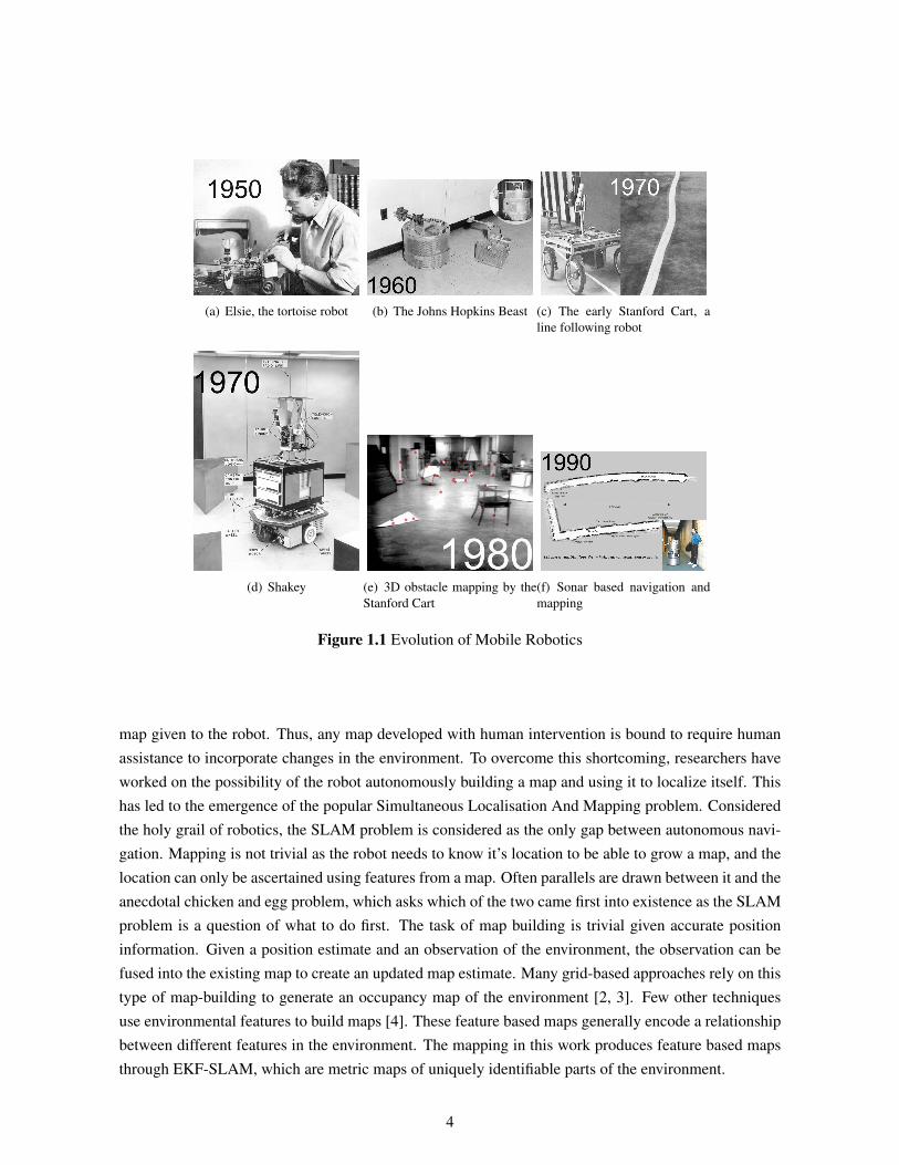
(a) Elsie, the tortoise robot (b) The Johns Hopkins Beast (c) The early Stanford Cart, aline following robot

(d) Shakey (e) 3D obstacle mapping by theStanford Cart

(f) Sonar based navigation andmapping

Figure 1.1 Evolution of Mobile Robotics

map given to the robot. Thus, any map developed with human intervention is bound to require humanassistance to incorporate changes in the environment. To overcome this shortcoming, researchers haveworked on the possibility of the robot autonomously building a map and using it to localize itself. Thishas led to the emergence of the popular Simultaneous Localisation And Mapping problem. Consideredthe holy grail of robotics, the SLAM problem is considered as the only gap between autonomous navi-gation. Mapping is not trivial as the robot needs to know it’s location to be able to grow a map, and thelocation can only be ascertained using features from a map. Often parallels are drawn between it and theanecdotal chicken and egg problem, which asks which of the two came first into existence as the SLAMproblem is a question of what to do first. The task of map building is trivial given accurate positioninformation. Given a position estimate and an observation of the environment, the observation can befused into the existing map to create an updated map estimate. Many grid-based approaches rely on thistype of map-building to generate an occupancy map of the environment [2, 3]. Few other techniquesuse environmental features to build maps [4]. These feature based maps generally encode a relationshipbetween different features in the environment. The mapping in this work produces feature based mapsthrough EKF-SLAM, which are metric maps of uniquely identifiable parts of the environment.

4

This work is primarily the result of a project funded by the Bhabha Atomic Research Centre(BARC),Mumbai, which plans to use the system and the knowledge acquired from this work in sensitive sur-roundings to replace human intervention. There are numerous areas prone to radioactivity in BARCand Variable Energy Cyclotron Centre(VECC), Kolkota. These areas require constant supervision byrobots to keep a check on radioactivity levels so that appropriate action can be taken upon sighting highlevels of radioactivity. Currently, the system in use utilizes a human operated robot to traverse aroundthe sensitive areas. The robot possesses a radioactivity level measuring instrument and through wirelessaccess transfers the acquired data periodically. A SLAM based deployment of this system is bound toreduce human effort by continuously traversing around the sensitive areas and reporting on finding highlevels of radioactivity. Also, a medical cyclotron is being constructed in VECC kolkota. This wouldrequire a large map to be regularly checked at all places for radioactivity. SLAM based solutions, uponbuilding a map, ensure a very robust performance and can solve the problem of patrolling and measuringradioactivity autonomously. These are just few of the innumerable areas that SLAM can bring mobilerobotics into.

1.2 Related Work

The genesis of the probabilistic SLAM problem occurred at the IEEE Robotics and AutomationConference in the year 1986. This was a time when probabilistic methods were on the verge of beingintroduced into robotics [5]. Table cloths and napkins were filled with long discussions by a number ofresearchers including Peter Cheeseman, Hugh Durrant-Whyte and Jim Crowley, who had been lookingat applying estimation theory based methods to the problem of mapping and localization. The resultof this conference was an understanding of the need of consistent probabilistic maps. Following theconference, a number of seminal papers were produced, which paved the way for a practical imple-mentation of autonomous mapping. Works by Leonard and Durrant-Whyte [6] and Smith et al [7], [8]explained a statistical basis for describing the spatial relationships between features. It was in this workthat the strong correlation between features in the map and the incremental growth of these correlationswas first shown. During the same time, Chatila and Laumond [9] were working on kalman filter typealgorithms for navigation based on sonar. It was eventually shown that as a mobile robot moves throughan unknown environment taking relative observations of landmarks, the estimates of these landmarksare all necessarily correlated with each other because of the common error in estimated vehicle location[6]. This implied that a consistent full solution to the SLAM problem would require repetitive updateof a joint state composed of the vehicle pose and every landmark location, with each new observationof the environment. These initial works did not consider the convergence properties of the map in asteady-state behaviour. Map errors were assumed to be growing without bounds rather than converging.This led to researchers shifting focus towards reducing the full filter to a series of decoupled landmarkto robot pose filters. The conceptual breakthrough came with the realization that the Mapping andLocalization problem, once formulated as a single problem, would be convergent. This structure and

5

formulation of the SLAM problem with the coining of the acronym came about by Durrant-Whyte etal [10]. Much of theoretical background on convergence was developed by Csorba [11]. During thesame time groups from Zaragoza [12, 13], MIT [14], ACFR and others were also working on the SLAMproblem. Thrun [15] introduced the convergence between kalman-filter based SLAM and probabilisticmethods for mapping and localization. After the conception of the SLAM theory, numerous approacheshave sprung up which deal with the map building process using novel and different techniques. TheExtended Kalman FIlter based SLAM, which has been used in this work is the most popular approachfor map building. The importance of this approach as compared to a Kalman filter remains in the abilityto represent non-linear models. This capability is very essential as almost all navigation problems canbe modelled as non-linear problems. However, highly non-linear problems tend to have erroneous ap-proximations and may cause the failure of an EKF based SLAM. This led to the idea of using UnscentedKalman FIlter based SLAM, by Julier and Uhlmann [16] which would perform better linearisation andtherefore improve map building by reducing errors. This was followed by FastSLAM, which uses parti-cle filter based techniques to perform map building. Errors due to non-linearity and high computationalcost led to a host of submap based SLAM algorithms that divide the map into local submaps which per-form partial updates. Novel approaches to the submap based SLAM process [17] claim to have furtherreduced the computational complexity to a constant while maintaining consistency. Recently, researchhas started shifting towards solving the SLAM problem using sparse optimization techniques [18] whichare of higher efficiency and yet also do not suffer from errors.

1.3 Contributions

This thesis can be broadly divided into two different kinds of contributions although both are inter-leaved to an extent. The primary contribution of this work remains in the implementation of a robust andscalable EKF-SLAM system deployment in real environments. This system is useful as a baseline forany further research and can be used as a testbed for comparisons and for further related research. Thedeployed system has also been shown to function on demand in different environments and on differentrobots with minimal overhead functionality issues(This system was deployed in VECC and the resultsare available in section 5.2.3). This deployment of a SLAM algorithm is to our knowledge, the first suchsystem developed in the country.

An in-house calibration system to align the laser frame of reference with the robots frame of referencehas been a very important breakthrough in the path of implementing an EKF-SLAM algorithm. Inspiteof the existence of successfully deployed SLAM systems, there has been scant or no mention of theimportance and requirement of calibration in the literature of mobile robotics with range scanners. Ournovel calibration scheme which considers all possible errors between the laser and the robots frameof reference, has played a major role in the success of our SLAM implementation by reducing errorsconsiderably. The calibration information gained thus, is directly useful for most projects that require

6

the range scanner and use the same robot and can prevent innumerable issues that might be encounteredin systems which might not show up any theoretical error.

The SLAM system has been deployed as two versions: The online EKF-SLAM and the offline EKF-SLAM. The online version runs a real-time SLAM algorithm on the Pioneer P3-Dx robot using a SICKLMS 200 laser range scanner. The online EKF-SLAM algorithm maintains the robot pose error andthe map in real-time to prevent the robot from straying away from its path. On the other hand, theoffline version of the algorithm has been developed to be tested against datasets containing robot poseinformation and raw range readings.

In the theoretical front, we have developed a smoothed EKF-SLAM algorithm which builds a com-plete metric map at low computational costs. A complete metric map, unlike a simple feature map, canbe utilized for path planning. This contribution helps in not only developing a feature map where therobot can localize, but also a full metric map for the robot to plan its path while avoiding obstacles.

This thesis also contributes in improving map building through the use of novel parametrization offeatures. Lines are used as features in environments with sparse point features to keep a check on therobot heading error which has resulted in better mapping results. A novel technique to use representativefeatures and to divide regions based on space has also been proposed in this thesis through which theprocess of map building can be made more intelligent.

1.4 Organization of this thesis

This thesis can be visualized as the amalgamation of three parts, namely:

• The structure of Extended Kalman Filter based SLAM

• Implementation of the EKF-SLAM algorithm on a real system

• Understanding and improving SLAM through features

The first part, the structure of the EKF-SLAM algorithm, explains the assumptions behind and thefunctionality of the EKF-SLAM algorithm which is a prerequisite before attempting to implement thealgorithm on a real system. These details have been discussed in Chapter 2.

The second part which involves the discussion of issues faced and resolved, customizations requiredfor implementation according to requirements and our calibration technique are elucidated in Chapter3. This chapter also includes a discussion on the smoothing of EKF-SLAM data for a complete metricmap.

The third part, Chapter 4, revolves around features, which form the backbone of the algorithm. Thispart deals with feature extraction, feature association and different feature representations. This partalso discusses novel feature combination techniques for better mapping and representative feature basedmapping for improving data association while also building a hybrid map with more information.

7

Experiments on Mapping and their corresponding results have been presented in Chapter 5. The ex-perimental results are a summary of the feature maps developed in various environments. The summaryof this work, with scope for future work has been discussed in Chapter 6.

8

Chapter 2

Simultaneous Localisation And Mapping

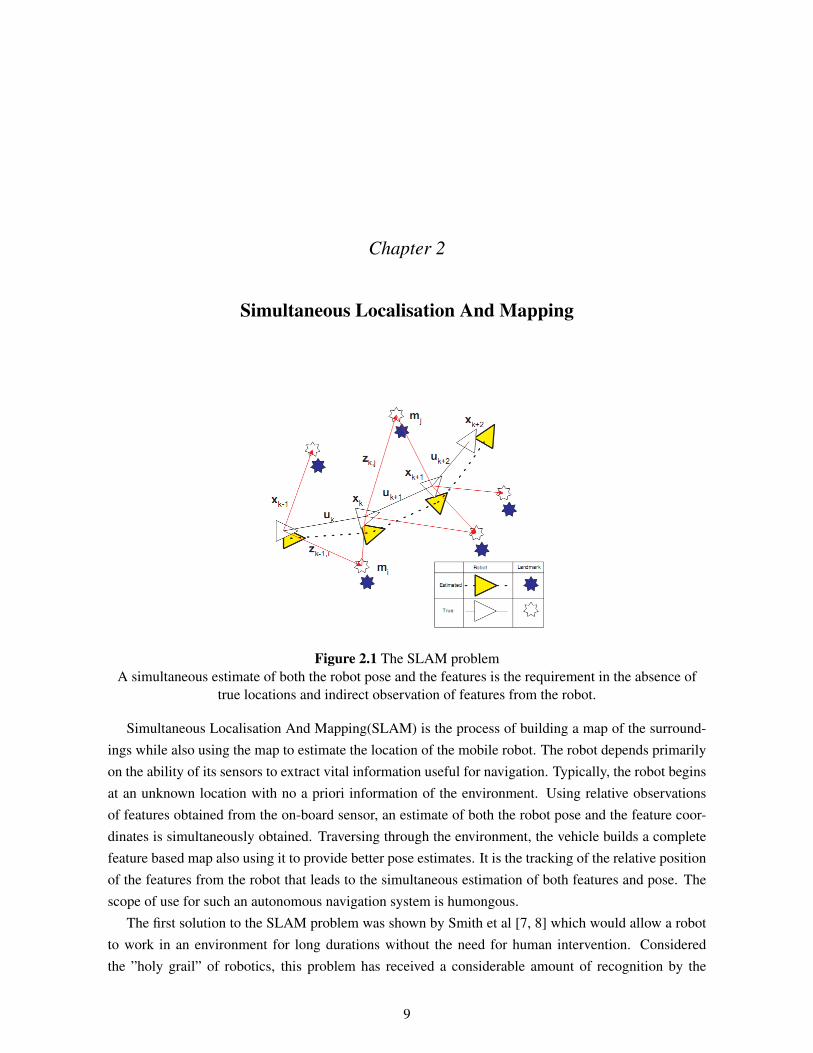
Figure 2.1 The SLAM problemA simultaneous estimate of both the robot pose and the features is the requirement in the absence of

true locations and indirect observation of features from the robot.

Simultaneous Localisation And Mapping(SLAM) is the process of building a map of the surround-ings while also using the map to estimate the location of the mobile robot. The robot depends primarilyon the ability of its sensors to extract vital information useful for navigation. Typically, the robot beginsat an unknown location with no a priori information of the environment. Using relative observationsof features obtained from the on-board sensor, an estimate of both the robot pose and the feature coor-dinates is simultaneously obtained. Traversing through the environment, the vehicle builds a completefeature based map also using it to provide better pose estimates. It is the tracking of the relative positionof the features from the robot that leads to the simultaneous estimation of both features and pose. Thescope of use for such an autonomous navigation system is humongous.

The first solution to the SLAM problem was shown by Smith et al [7, 8] which would allow a robotto work in an environment for long durations without the need for human intervention. Consideredthe ”holy grail” of robotics, this problem has received a considerable amount of recognition by the

9

mobile robotics community as a stepping stone towards autonomous navigation. This work primarilyis about stochastic estimation techniques to build and maintain the map coordinates and the robot pose.In particular, the SLAM algorithm has been implemented using an Extended Kalman Filter(EKF) basedalgorithm to map the environment.

While the Kalman filter based SLAM has received immense interest, alternative methods to tackleSLAM also appear in literature. A number of research groups have worked on particle filter basedmethods, while some groups have done away with the rigorous mathematical models and have reliedon a more qualitative information of the environment. Also, quite a few people have tackled the SLAMproblem using batch estimation techniques. While all of these alternative approaches have their ownmerits, this thesis concentrates solely on EKF based SLAM to provide autonomous navigation.

2.1 Introduction

The EKF SLAM approach to slam is to develop a filtering process for the system. This thesis dealswith two-dimensional SLAM in a three-dimensional environment, which is done by using the rangescanner which cuts the environment into a two-dimensional plane. Thus, the map is represented as atwo dimensional map. This also adds the underlying assumption of having obstacles in the environmentwhich are orthogonal to the ground plane.

The system which is to be modelled, is a discrete time system, with a variable state represented by avector. The variables in the state vector can change over time, hence the system is dynamic. However,the system possesses fixed rules for the evolution of the state which describe what future states willfollow from the current state.

The EKF-SLAM system is similar to the estimation of a linear dynamic system, save a few con-straints that increase its complexity. Therefore, the SLAM system is shown in this work as an extensionof the generic estimation algorithm for the estimation of a linear dynamic system.

A basic overview of probability concepts that were felt necessary for understanding the functioningof the system are covered in the Appendix A.

2.2 Estimation of a Dynamic System

A dynamic system is defined as a system whose state can vary with time according to fixed rulesfor its evolution. A linear dynamic system is one in which the evolution rule from the current state to afuture state is a linear transformation. Evidently, we will model a stochastic process B.1, also called arandom process, by virtue of the random variables which affect the state evolution.

Our system samples information and processes it to estimate its state. This information is non-continuous, or discrete. So, a simple model of a system very similar to the required one, would be thatof a discrete-time linear stochastic dynamic system.

10

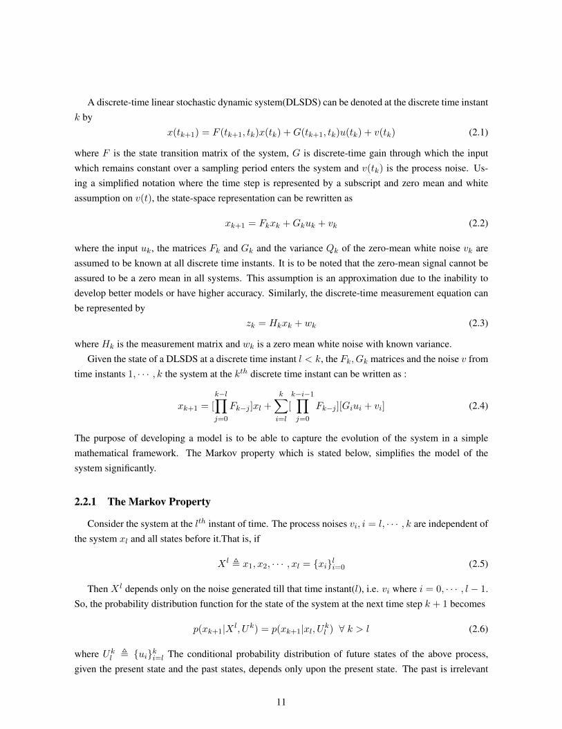
A discrete-time linear stochastic dynamic system(DLSDS) can be denoted at the discrete time instantk by

x(tk+1) = F (tk+1, tk)x(tk) +G(tk+1, tk)u(tk) + v(tk) (2.1)

where F is the state transition matrix of the system, G is discrete-time gain through which the inputwhich remains constant over a sampling period enters the system and v(tk) is the process noise. Us-ing a simplified notation where the time step is represented by a subscript and zero mean and whiteassumption on v(t), the state-space representation can be rewritten as

xk+1 = Fkxk +Gkuk + vk (2.2)

where the input uk, the matrices Fk and Gk and the variance Qk of the zero-mean white noise vk areassumed to be known at all discrete time instants. It is to be noted that the zero-mean signal cannot beassured to be a zero mean in all systems. This assumption is an approximation due to the inability todevelop better models or have higher accuracy. Similarly, the discrete-time measurement equation canbe represented by

zk = Hkxk + wk (2.3)

where Hk is the measurement matrix and wk is a zero mean white noise with known variance.Given the state of a DLSDS at a discrete time instant l < k, the Fk, Gk matrices and the noise v from

time instants 1, · · · , k the system at the kth discrete time instant can be written as :

xk+1 = [

k−l∏j=0

Fk−j ]xl +

k∑i=l

[

k−i−1∏j=0

Fk−j ][Giui + vi] (2.4)

The purpose of developing a model is to be able to capture the evolution of the system in a simplemathematical framework. The Markov property which is stated below, simplifies the model of thesystem significantly.

2.2.1 The Markov Property

Consider the system at the lth instant of time. The process noises vi, i = l, · · · , k are independent ofthe system xl and all states before it.That is, if

X l , x1, x2, · · · , xl = {xi}li=0 (2.5)

Then X l depends only on the noise generated till that time instant(l), i.e. vi where i = 0, · · · , l − 1.So, the probability distribution function for the state of the system at the next time step k + 1 becomes

p(xk+1|X l, Uk) = p(xk+1|xl, Ukl ) ∀ k > l (2.6)

where Ukl , {ui}ki=l The conditional probability distribution of future states of the above process,given the present state and the past states, depends only upon the present state. The past is irrelevant

11

because it does not matter how the current state was obtained, just that the current state encompassesall information necessary to estimate the next state. This property is called the Markov property and aprocess with the property is called a Markov process.

Given the current state of a DLSDS, the control input and the error, all the past states, their controlinputs and their process errors are not required to predict the next state. This property is used as the baseto model the evolution of such a system.

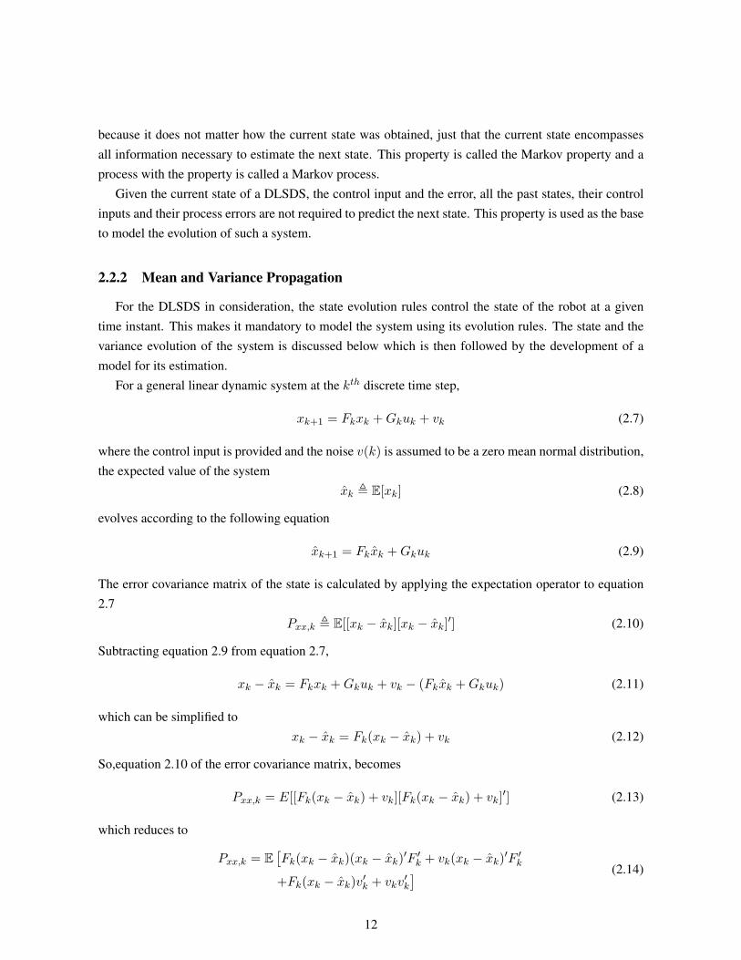
2.2.2 Mean and Variance Propagation

For the DLSDS in consideration, the state evolution rules control the state of the robot at a giventime instant. This makes it mandatory to model the system using its evolution rules. The state and thevariance evolution of the system is discussed below which is then followed by the development of amodel for its estimation.

For a general linear dynamic system at the kth discrete time step,

xk+1 = Fkxk +Gkuk + vk (2.7)

where the control input is provided and the noise v(k) is assumed to be a zero mean normal distribution,the expected value of the system

xk , E[xk] (2.8)

evolves according to the following equation

xk+1 = Fkxk +Gkuk (2.9)

The error covariance matrix of the state is calculated by applying the expectation operator to equation2.7

Pxx,k , E[[xk − xk][xk − xk]′] (2.10)

Subtracting equation 2.9 from equation 2.7,

xk − xk = Fkxk +Gkuk + vk − (Fkxk +Gkuk) (2.11)

which can be simplified toxk − xk = Fk(xk − xk) + vk (2.12)

So,equation 2.10 of the error covariance matrix, becomes

Pxx,k = E[[Fk(xk − xk) + vk][Fk(xk − xk) + vk]′] (2.13)

which reduces to

Pxx,k = E[Fk(xk − xk)(xk − xk)′F ′k + vk(xk − xk)′F ′k

+Fk(xk − xk)v′k + vkv′k

] (2.14)

12

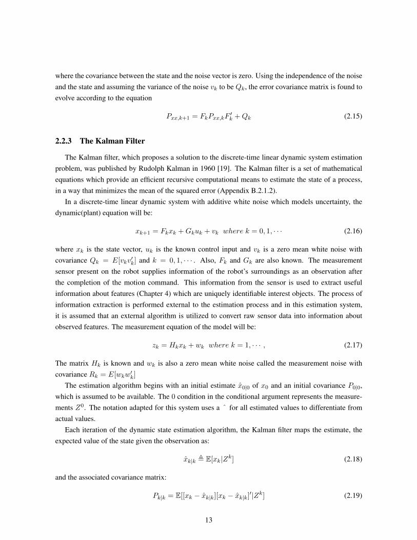
where the covariance between the state and the noise vector is zero. Using the independence of the noiseand the state and assuming the variance of the noise vk to be Qk, the error covariance matrix is found toevolve according to the equation

Pxx,k+1 = FkPxx,kF′k +Qk (2.15)

2.2.3 The Kalman Filter

The Kalman filter, which proposes a solution to the discrete-time linear dynamic system estimationproblem, was published by Rudolph Kalman in 1960 [19]. The Kalman filter is a set of mathematicalequations which provide an efficient recursive computational means to estimate the state of a process,in a way that minimizes the mean of the squared error (Appendix B.2.1.2).

In a discrete-time linear dynamic system with additive white noise which models uncertainty, thedynamic(plant) equation will be:

xk+1 = Fkxk +Gkuk + vk where k = 0, 1, · · · (2.16)

where xk is the state vector, uk is the known control input and vk is a zero mean white noise withcovariance Qk = E[vkv

′k] and k = 0, 1, · · · . Also, Fk and Gk are also known. The measurement

sensor present on the robot supplies information of the robot’s surroundings as an observation afterthe completion of the motion command. This information from the sensor is used to extract usefulinformation about features (Chapter 4) which are uniquely identifiable interest objects. The process ofinformation extraction is performed external to the estimation process and in this estimation system,it is assumed that an external algorithm is utilized to convert raw sensor data into information aboutobserved features. The measurement equation of the model will be:

zk = Hkxk + wk where k = 1, · · · , (2.17)

The matrix Hk is known and wk is also a zero mean white noise called the measurement noise withcovariance Rk = E[wkw

′k]

The estimation algorithm begins with an initial estimate x0|0 of x0 and an initial covariance P0|0,which is assumed to be available. The 0 condition in the conditional argument represents the measure-ments Z0. The notation adapted for this system uses a ˆ for all estimated values to differentiate fromactual values.

Each iteration of the dynamic state estimation algorithm, the Kalman filter maps the estimate, theexpected value of the state given the observation as:

xk|k , E[xk|Zk] (2.18)

and the associated covariance matrix:

Pk|k = E[[xk − xk|k][xk − xk|k]′|Zk] (2.19)

13

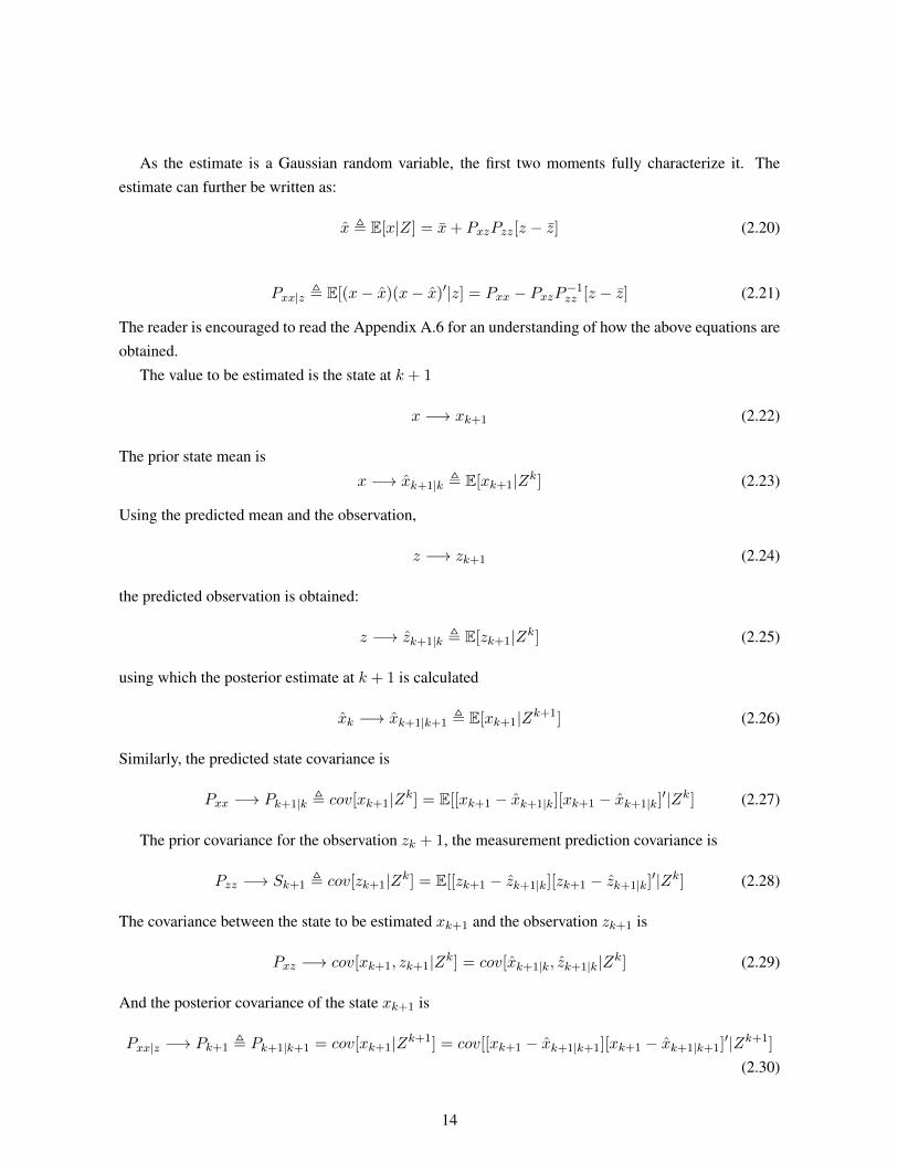
As the estimate is a Gaussian random variable, the first two moments fully characterize it. Theestimate can further be written as:

x , E[x|Z] = x+ PxzPzz[z − z] (2.20)

Pxx|z , E[(x− x)(x− x)′|z] = Pxx − PxzP−1zz [z − z] (2.21)

The reader is encouraged to read the Appendix A.6 for an understanding of how the above equations areobtained.

The value to be estimated is the state at k + 1

x −→ xk+1 (2.22)

The prior state mean is

x −→ xk+1|k , E[xk+1|Zk] (2.23)

Using the predicted mean and the observation,

z −→ zk+1 (2.24)

the predicted observation is obtained:

z −→ zk+1|k , E[zk+1|Zk] (2.25)

using which the posterior estimate at k + 1 is calculated

xk −→ xk+1|k+1 , E[xk+1|Zk+1] (2.26)

Similarly, the predicted state covariance is

Pxx −→ Pk+1|k , cov[xk+1|Zk] = E[[xk+1 − xk+1|k][xk+1 − xk+1|k]′|Zk] (2.27)

The prior covariance for the observation zk + 1, the measurement prediction covariance is

Pzz −→ Sk+1 , cov[zk+1|Zk] = E[[zk+1 − zk+1|k][zk+1 − zk+1|k]′|Zk] (2.28)

The covariance between the state to be estimated xk+1 and the observation zk+1 is

Pxz −→ cov[xk+1, zk+1|Zk] = cov[xk+1|k, zk+1|k|Zk] (2.29)

And the posterior covariance of the state xk+1 is

Pxx|z −→ Pk+1 , Pk+1|k+1 = cov[xk+1|Zk+1] = cov[[xk+1 − xk+1|k+1][xk+1 − xk+1|k+1]′|Zk+1]

(2.30)

14

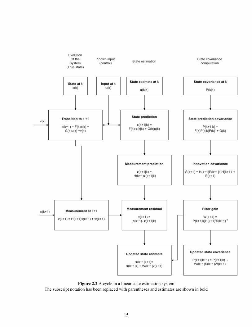
Figure 2.2 A cycle in a linear state estimation systemThe subscript notation has been replaced with parentheses and estimates are shown in bold

15

2.3 The EKF-SLAM Model

Our system uses an Extended Kalman Filter based SLAM which is an extension of the Kalman filterdiscussed previously as the name suggests. The Kalman filter deals with only linear systems. However,most navigational problems as the SLAM problem, have non-linear models which renders the directusage of a Kalman filter not possible. Numerous methods are used to deal with the non-linearity indifferent SLAM algorithms. An Extended Kalman Filter, one of the more popular methods for handlingnon-linearity, expects the system models to be differentiable and linearizes the non-linear functionsaround the current estimates.

The only difference in the Extended Kalman Filter is that the state transition and the observationequations are no longer linear functions in the process, so they are linearized by the first order Taylorseries approximation by the use of a Jacobian. The SLAM algorithm differs from the Kalman andExtended Kalman filtering algorithms by the use of a joint state that also includes observations.

2.3.1 The State Vector

The SLAM algorithm utilizes a single joint vector random variable consisting of both the pose esti-mate of the robot and the feature estimates. The robot traverses through the environment, all the whilesensing features that are visible and discernible. The state vector, is hence, not of a constant size. Rather,the size of the state vector keeps incrementing with the observation of new features that do not matchwith previously seen features. The state of the system at time k will be represented by the state vec-tor x(k), consisting of vn scalar random variables for the robot pose estimate, and fn vector randomvariables, each of the fn variables representing the pose estimate of one unique feature.

xk =

xv,k

xf1,k

.

.

.

xfn,k

(2.31)

where all the coordinates xi,k in the state are denoted relative to the global frame of reference. Accordingto the terminology established by Newman [20], the SLAM algorithm in which all state estimates arewith respect to a common, global frame of reference is referred to as the Absoulte Map Filter(AMF). Itis to be noted that since all states are taken to be with respect to a global reference frame, no notationhas been denoted to classify variables in the global frame of reference.

The cumulative state vector can be also be expressed by dividing it into two parts, the robot posevector and the feature vector :

xk =

[xv,k

xm,k

](2.32)

16

where xv,k is the robot pose vector and xm,k is the map vector, the vector of all features in the map.The robot is considered an Autonomous Ground Vehicle(AGV), so it travels only in the two-dimensionalplane, and its location can be represented using two scalars. However, the robot also possesses a headingwhich also needs to be represented in the robot pose. Thus,

xv,k =

xv,kyv,k

θv,k

(2.33)

where xv,k, yv,kandθv,k represent the mean estimate along the x-axis, y-axis and the heading with re-spect to the global frame of reference respectively.

The features xfi,k can be defined in the map by a position in the two dimensional space

xfi,k =

[xfi,k

yfi,k

](2.34)

and the map vector is

xm,k =

xf1,k

.

.

.

xfn,k

(2.35)

2.3.2 Vehicle Motion Model

The vehicle motion model or simply motion model, captures the fundamental relationship betweenthe robot’s past state, xv,k, and current state, xv,k+1, given the control input, uk

xv,k = fv,k(xv,k−1,uk,vu,k) (2.36)

An accurate motion model is an important requirement for a good navigation scheme. However,as realistic vehicles always suffer from noise, any vehicle model is bound to have errors creeping indue to noise. Two widely popular motion models are generally adapted to suit most requirements:the odometry based motion model and the velocity based motion model. The odometry based motionmodel is popular with most commercial bases which provide odometry using kinematic information.The odometry based motion model provides the distance travelled and the angle turned by the robot. Onthe other hand, the velocity based motion model assumes that independent translational and rotationalvelocities are specified to the robot motors and the motion is performed for the desired time to reach thedestination.

In practise, odometry models are observed to be more accurate than velocity based models. This canbe attributed to the fact that most commercial robots do not execute velocity based commands with thelevel of accuracy that can be achieved by measuring the revolution of the robot’s wheels. The problem

17

with odometry is however, that it is only available after the motion command has been executed. So, itcannot be used for motion planning methods where prediction of the effects of the motion is requiredfor collision avoidance.

In this work, an odometry based motion model has been used. The model uses as inputs, the pastestimate of the robot pose, xv,k|k, and the control input, uk and produces as output the current meanprediction of the robot pose.xv,k+1|k

yv,k+1|k

θv,k+1|k

=

xv,k+1|k + ru,k cos(θv,k + θu,k)

yv,k+1|k + ru,k sin(θv,k + θu,k)

θv,k + θu,k

(2.37)

The scalars ruu, k and θu,k are part of the control command, uk, issued to the robot.

uk =

[ru,k

θu,k

](2.38)

System-dependent details have been excluded from this chapter and will be discussed in the next chap-ter 3.

2.3.3 Feature Model

A feature in SLAM terminology, is a part of the environment which can be observed reliably usingthe robot’s sensors. Features must be described in a parametric form for them to be incorporated intoa state model. Point landmarks, corners, line and polyline feature models have all been used in SLAMliterature [21], [22], [23], [24]. The scope of this work applies only to static environments which impliesthat the features shall be assumed to be stationary. Thus, it is only the robot pose vector in the state whichis dynamic in nature. That is, the feature model is simply

xm,k = xm,k−1 (2.39)

where xm,k are the feature estimates at time instant k.

2.3.4 Sensor Measurement Model

Measurement models describe the formation process by which the sensor measures in the physicalworld. Today’s robots use a variety of different sensor modalities like tactile sensors, range sensors orcameras. The state observation can be modelled as

zk = h(xk) + wk (2.40)

where zk ∈ Rfn is the observation at time k. and h is a model of the observation of the system states asa function of time and w(k) is a random vector describing the measurement noise and uncertainties inthe model.

18

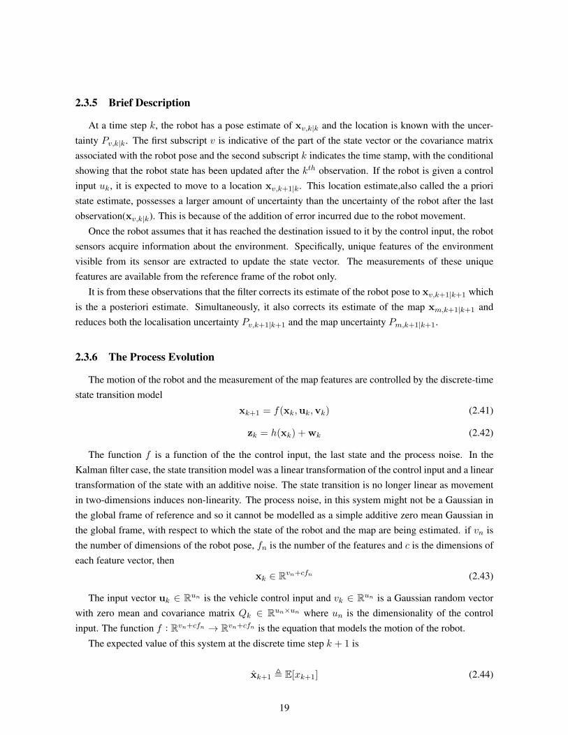
2.3.5 Brief Description

At a time step k, the robot has a pose estimate of xv,k|k and the location is known with the uncer-tainty Pv,k|k. The first subscript v is indicative of the part of the state vector or the covariance matrixassociated with the robot pose and the second subscript k indicates the time stamp, with the conditionalshowing that the robot state has been updated after the kth observation. If the robot is given a controlinput uk, it is expected to move to a location xv,k+1|k. This location estimate,also called the a prioristate estimate, possesses a larger amount of uncertainty than the uncertainty of the robot after the lastobservation(xv,k|k). This is because of the addition of error incurred due to the robot movement.

Once the robot assumes that it has reached the destination issued to it by the control input, the robotsensors acquire information about the environment. Specifically, unique features of the environmentvisible from its sensor are extracted to update the state vector. The measurements of these uniquefeatures are available from the reference frame of the robot only.

It is from these observations that the filter corrects its estimate of the robot pose to xv,k+1|k+1 whichis the a posteriori estimate. Simultaneously, it also corrects its estimate of the map xm,k+1|k+1 andreduces both the localisation uncertainty Pv,k+1|k+1 and the map uncertainty Pm,k+1|k+1.

2.3.6 The Process Evolution

The motion of the robot and the measurement of the map features are controlled by the discrete-timestate transition model

xk+1 = f(xk,uk,vk) (2.41)

zk = h(xk) + wk (2.42)

The function f is a function of the the control input, the last state and the process noise. In theKalman filter case, the state transition model was a linear transformation of the control input and a lineartransformation of the state with an additive noise. The state transition is no longer linear as movementin two-dimensions induces non-linearity. The process noise, in this system might not be a Gaussian inthe global frame of reference and so it cannot be modelled as a simple additive zero mean Gaussian inthe global frame, with respect to which the state of the robot and the map are being estimated. if vn isthe number of dimensions of the robot pose, fn is the number of the features and c is the dimensions ofeach feature vector, then

xk ∈ Rvn+cfn (2.43)

The input vector uk ∈ Run is the vehicle control input and vk ∈ Run is a Gaussian random vectorwith zero mean and covariance matrix Qk ∈ Run×un where un is the dimensionality of the controlinput. The function f : Rvn+cfn → Rvn+cfn is the equation that models the motion of the robot.

The expected value of this system at the discrete time step k + 1 is

xk+1 , E[xk+1] (2.44)

19

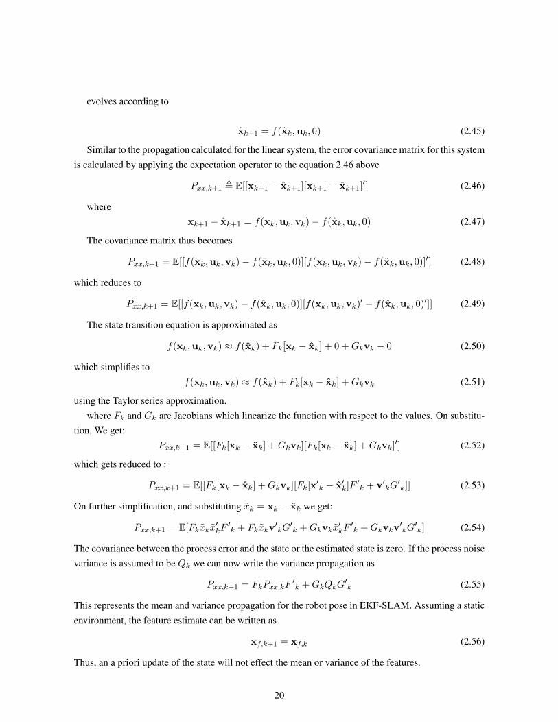
evolves according to

xk+1 = f(xk,uk, 0) (2.45)

Similar to the propagation calculated for the linear system, the error covariance matrix for this systemis calculated by applying the expectation operator to the equation 2.46 above

Pxx,k+1 , E[[xk+1 − xk+1][xk+1 − xk+1]′] (2.46)

wherexk+1 − xk+1 = f(xk,uk,vk)− f(xk,uk, 0) (2.47)

The covariance matrix thus becomes

Pxx,k+1 = E[[f(xk,uk,vk)− f(xk,uk, 0)][f(xk,uk,vk)− f(xk,uk, 0)]′] (2.48)

which reduces to

Pxx,k+1 = E[[f(xk,uk,vk)− f(xk,uk, 0)][f(xk,uk,vk)′ − f(xk,uk, 0)′]] (2.49)

The state transition equation is approximated as

f(xk,uk,vk) ≈ f(xk) + Fk[xk − xk] + 0 +Gkvk − 0 (2.50)

which simplifies tof(xk,uk,vk) ≈ f(xk) + Fk[xk − xk] +Gkvk (2.51)

using the Taylor series approximation.where Fk and Gk are Jacobians which linearize the function with respect to the values. On substitu-

tion, We get:Pxx,k+1 = E[[Fk[xk − xk] +Gkvk][Fk[xk − xk] +Gkvk]

′] (2.52)

which gets reduced to :

Pxx,k+1 = E[[Fk[xk − xk] +Gkvk][Fk[x′k − x′k]F

′k + v′kG

′k]] (2.53)

On further simplification, and substituting xk = xk − xk we get:

Pxx,k+1 = E[Fkxkx′kF′k + Fkxkv

′kG′k +Gkvkx

′kF′k +Gkvkv

′kG′k] (2.54)

The covariance between the process error and the state or the estimated state is zero. If the process noisevariance is assumed to be Qk we can now write the variance propagation as

Pxx,k+1 = FkPxx,kF′k +GkQkG

′k (2.55)

This represents the mean and variance propagation for the robot pose in EKF-SLAM. Assuming a staticenvironment, the feature estimate can be written as

xf,k+1 = xf,k (2.56)

Thus, an a priori update of the state will not effect the mean or variance of the features.

20

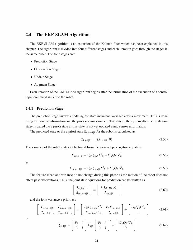
2.4 The EKF-SLAM Algorithm

The EKF-SLAM algorithm is an extension of the Kalman filter which has been explained in thischapter. The algorithm is divided into four different stages and each iteration goes through the stages inthe same order. The four stages are:

• Prediction Stage

• Observation Stage

• Update Stage

• Augment Stage

Each iteration of the EKF-SLAM algorithm begins after the termination of the execution of a controlinput command issued to the robot.

2.4.1 Prediction Stage

The prediction stage involves updating the state mean and variance after a movement. This is doneusing the control information and the process error variance. The state of the system after the predictionstage is called the a priori state as this state is not yet updated using sensor information.

The predicted state or the a priori state xv,k+1|k for the robot is calculated as

xk+1|k = f(xk,uk,0) (2.57)

The variance of the robot state can be found from the variance propagation equation:

Pxx,k+1 = FkPxx,kF′k +GkQkG

′k (2.58)

asPvv,k+1|k = FkPvv,k|kF

′k +GkQkG

′k (2.59)

The feature mean and variance do not change during this phase as the motion of the robot does noteffect past observations. Thus, the joint state equations for prediction can be written as[

xv,k+1|k

xm,k+1|k

]=

[f(xk,uk,0)

xm,k|k

](2.60)

and the joint variance a priori as :[Pvv,k+1|k Pvm,k+1|k

Pmv,k+1|k Pmm,k+1|k

]=

[FkPvv,k|kF

′k FkPvm,k|k

Pmv,k|kF′k Pmm,k|k

]+

[GkQkG

′k

0

](2.61)

or

Pk+1|k =

[Fk 0

0 I

]Pk|k

[Fk 0

0 I

]′+

[GkQkG

′k

0

](2.62)

21

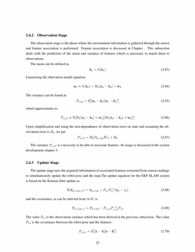
2.4.2 Observation Stage

The observation stage is the phase where the environment information is gathered through the sensorand feature association is performed. Feature association is discussed in Chapter . This subsectiondeals with the prediction of the mean and variance of features which is necessary to match them toobservations.

The mean can be defined as

zk = h(xk) (2.63)

Linearizing the obervation model equation,

zk ≈ h(xk) +Hk[xk − xk] + wk (2.64)

The variance can be found as

Pzz,k = E[[zk − zk][zk − zk]′] (2.65)

which approximates to

Pzz,k ≈ E[Hk[xk − xk] + wk][Hk[xk − xk] + wk]′] (2.66)

Upon simplification and using the non-dependence of observation error on state and assuming the ob-servation error is Rk, we get

Pzz,k = HkPk+1|kH′k +Rk (2.67)

The variance Pzz,k is a necessity to be able to associate features. Its usage is discussed in the systemdevelopment chapter 3.

2.4.3 Update Stage

The update stage uses the acquired information of associated features extracted from sensor readingsto simultaneously update the robot pose and the map.The update equation for the EKF-SLAM systemis based on the Kalman filter update as

E(xk+1|k+1) = xk+1|k + PxzP−1zz (zk − zk) (2.68)

and the covariance, as can be inferred from A.47, is

Pk+1|k+1 = Pk+1|k − Pxz,kP−1zz,kPzx (2.69)

The value Pzz is the observation variance which has been derived in the previous subsection. The valuePxz is the covariance between the robot pose and the features:

Pxz|z = E[[x− x][z− z]′] (2.70)

22

This can be rewritten using the linearized observation equation 2.64 as

Pxz|z = E[[xk+1 − xk+1|k][Hk[xk − xk+1|k] + wk]′] (2.71)

which upon simplification and removing terms with no covariance with the observation noise simplifiesto:

Pxz|z = Pxx|zH′k (2.72)

Similarly,

Pzx|z = E[[z− z][x− x]′] (2.73)

which simplifies to

Pzx|z = HkPxx|z (2.74)

The mean updated can now be rewritten as

E(xk+1|k+1) = xk+1|k + Pxx|zH′k(HkPk+1|kH

′k +Rk)

−1(zk − zk) (2.75)

Substitution of the factor by which the innovation effects the state by the value K, the Kalman gain:

E(xk+1|k+1) = xk+1|k +K(zk − zk) (2.76)

The updated covariance can be rewritten as

Pk+1|k+1 = Pk+1|k − Pxx|zH′k(HkPk+1|kH

′k +Rk)

−1HkPxx|z (2.77)

On simplification by substituting the Kalman gain,

Pk+1|k+1 = Pk+1|k −KHkPxx|z (2.78)

This can be written as:

Pk+1|k+1 = (I −KHk)Pk+1|k (2.79)

2.4.4 Augment Stage

The Augment stage in each iteration of the SLAM algorithm augments unmatched observations asnew features in the state vector. An observation z is in the form of (r, θ) from the reference frame ofthe robot. However, the observation cannot be directly added to the state vector as the state vector isrepresented in the global frame of reference and the local reference frame is not save or estimated. Thus,the feature is added into the state as:

xfj = m(z, xk) (2.80)

where xv is the robot pose estimate after the update in the same iteration.

23

The variance matrix also needs to be populated with the values corresponding to the added featurein the state. To find the variance, we use the Taylor series approximation of the observation:

xfj ≈ m(z, xk) +M [xk − xk] +N [yk] (2.81)

where M and N are the Jacobians for the pose and the error respectively. Upon Simplification, thevariance of the feature is found as:

Pfj = MPM ′ +NRN ′ (2.82)

The new covariance rows are added into the matrix as[MPvv MPvm Pfj = MPM ′ +NRN ′

](2.83)

More details about feature augmentation are discussed in detail in the section 4.2.4.

24

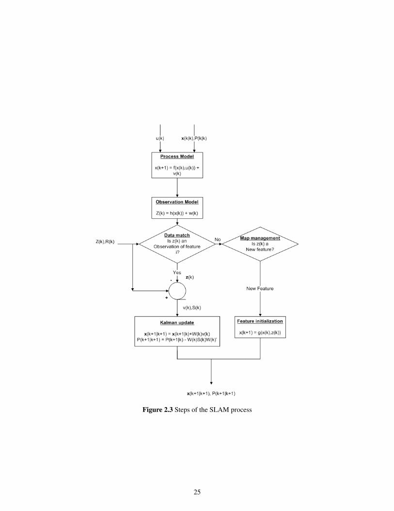
Figure 2.3 Steps of the SLAM process

25

2.5 Summary

The section discussed the probabilistic Kalman filter based SLAM algorithm. Specifically, the evo-lution of a linear dynamic system and its estimation has been discussed initially to assist in the under-standing of the non-linear dynamic system in consideration.

This is followed by an introduction to the Kalman filter which is the platform for the development ofthe SLAM algorithm employed in this work. The Extended Kalman Filter(EKF), which is essentially aKalman filter, but with the additional capability to handle non-linear data is employed in our system dueto the inherent non-linearities present in it. The EKF based SLAM system is discussed in the rest of thechapter and the equations for mean and variance estimation in each iteration of the algorithm have beendiscussed.

The EKF-SLAM algorithm estimates the mean and variance for the state of a nonlinear dynamicsystem by linearizing its values using a first order Taylor series approximation as a Jacobian due to themulti-variate property of the system. The mean of the robot pose and the mean of feature estimates inthe map are present in the state vector and their respective variances in the covariance matrix. Eachiteration of the algorithm is divided into four stages:

• Prediction

• Observation

• Update

• Augment

The robot is given a control input at the beginning of each iteration, following which its new poseand variance is predicted in the prediction stage. Following the prediction stage, range scanner data isrequested by the robot and the relevant features are extracted from the raw data. The features present inthe state vector are then associated with the observed features in the observation stage. The final stagecalled the update stage, uses the acquired information of current observations which are matched toalready observed features present in the state, to update the joint state vector and the covariance matrixthus updating the robot pose estimate and also the map estimate.

26

Chapter 3

System Development

This chapter presents the core development concepts, including engineering issues that have beenidentified and diagnosed to build a realistic EKF-SLAM model. The primary concern of this part ofthe work is to adapt the EKF-SLAM system to the required model and to develop the system to workin real-time. Concisely, the journey from theory to prototype, and the evolution of novel requirementswhich required to be handled are explained in detail.

The first part of this chapter develops models specific to the system to work with EKF-SLAM. Thissection discusses the motion model and the observation model developed for the system. The nextpart discusses the need for calibration of the sensor with respect to the robot and the development of acalibration system to be able to transform the coordinates in the sensor frame of reference to the robot’sframe of reference. The remainder of this chapter deals with different deployments of the system andtheir necessity concluding with a smoothing of the EKF-SLAM results to obtain the robot trajectoryestimate.

3.1 The Test-bed

Manufactured by Mobile Robots Inc, the robot used in the work, Pioneer P3-DX, is a popular mobilerobotics research platform. Like most popular indoor robots, the Pioneer P3-Dx does not move like acar. There are two main wheels, each of which is attached to its own motor. A third wheel(caster) isplaced in the rear to passively roll along while preventing the robot from falling over. As suggested bythe name, the robot has a differential drive. The version of Pioneer P3-Dx being used does not comewith an integrated computer system on-board to be able to access information and relay control inputs tothe robot. However, a serial port is present in the system through which relevant information is relayedto and collected from the robot. A SICK LMS 200 range scanner has been mounted on the Pioneer P3-Dx which provides environmental information to the system. The SICK LMS 200, like all laser sensors,operates by shining a laser off of a rotating mirror. As the mirror spins, the laser scans 180◦, effectivelycreating a fan of laser light. Any object that breaks this fan reflects laser light back to the sensor. The

27

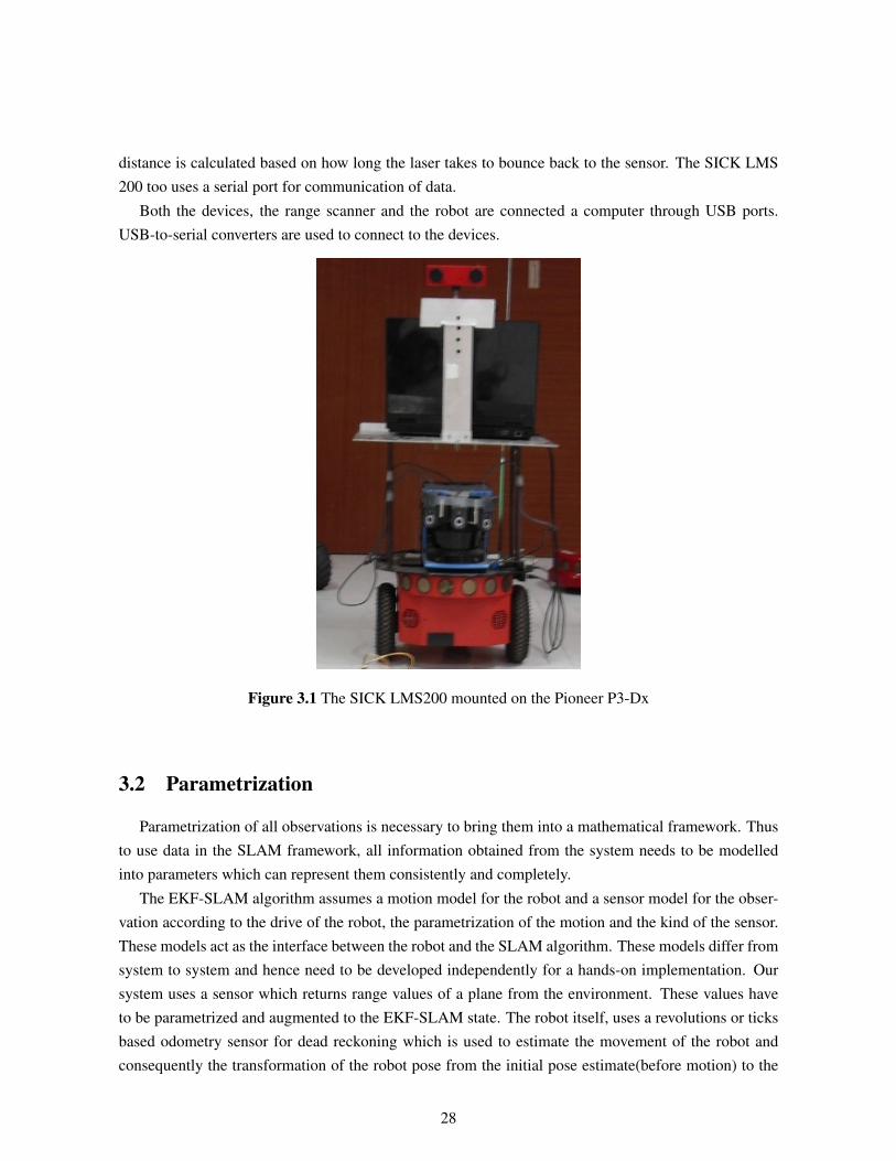
distance is calculated based on how long the laser takes to bounce back to the sensor. The SICK LMS200 too uses a serial port for communication of data.

Both the devices, the range scanner and the robot are connected a computer through USB ports.USB-to-serial converters are used to connect to the devices.

Figure 3.1 The SICK LMS200 mounted on the Pioneer P3-Dx

3.2 Parametrization

Parametrization of all observations is necessary to bring them into a mathematical framework. Thusto use data in the SLAM framework, all information obtained from the system needs to be modelledinto parameters which can represent them consistently and completely.

The EKF-SLAM algorithm assumes a motion model for the robot and a sensor model for the obser-vation according to the drive of the robot, the parametrization of the motion and the kind of the sensor.These models act as the interface between the robot and the SLAM algorithm. These models differ fromsystem to system and hence need to be developed independently for a hands-on implementation. Oursystem uses a sensor which returns range values of a plane from the environment. These values haveto be parametrized and augmented to the EKF-SLAM state. The robot itself, uses a revolutions or ticksbased odometry sensor for dead reckoning which is used to estimate the movement of the robot andconsequently the transformation of the robot pose from the initial pose estimate(before motion) to the

28

current pose estimate. This section gives an overview of the parametrization of the sensor values andthe motion values as required for inclusion into the SLAM state and for the state transition function.

3.2.1 Motion Model

A motion model uses the kinematics of the robot to predict its future pose estimate, given the currentposition of the robot and a control input. Thus, given a system with the equation:

xv,k+1 = fv,k(xv,k,uk,vu,k) (3.1)

a state transition model according to the control input would be:

xv,k+1|k = fv,k(xv,k,uk+1, 0) (3.2)

We use an odometry based motion model to predict the next pose of the robot. An odometry basedmotion model takes as input the previous pose estimate of the robot, the distance travelled by the robotor the angle turned by the robot, and returns the new pose estimate of the robot. It is to be noted that onlyone of either translation or rotation is to be given as control input in a single iteration of the algorithm.This is essential because the order of application of the given control input might not be certain. In otherwords, a unique transformation of the robot is not guaranteed if given two inputs, one of translation andone of rotation, without any prior precedence assignment.

However, our model does not use a control input directly issued to it to find it’s predicted state. Wehave developed a feedback system that determines with a higher degree of accuracy the control inputcommand given to the robot. There are three primary reasons for the need of such a model:

• The system to be developed assumes an external exploration algorithm. To suffice this constraint,a human operator controls the robot over the map. It is not feasible for a human operator to feedcontrol inputs every iteration to move the robot safely in an efficient way.

• Moreover, a major observation from the initial system testing was the inaccuracy of the robot toreach the point issued to it by the control input. The reason for this error is out of the scope of thiswork. However, a query to the robot server(through the API) would return pose estimates withhigher accuracy.

• Often control commands issues to the robot less than half a meter would result in erratic move-ments with no discernible pattern making it tough to model the actual movement.

Our algorithm utilizes a joystick based control of the robot in which case there is no prior control inputgiven to the robot but the robot itself is driven from one point to another. Therefore, the predicted posexv,k+1|k, in this case, need not be calculated from a function of the control input. Rather, the predictedpose of the robot after the motion command is readily available. However, there is still a need to modelxv,k+1|k as a function of the previous state xv,k and the control uk. We have the transformation

uk+1 = A(xv,k+1|k, xv,k) (3.3)

29

The state transition function for prediction plays a key role in the EKF-SLAM model. It is the Jacobianderived from this function, that is used to update the covariance matrix.

Pk+1|k = FkPk|kF′k +GkQk+1Gk (3.4)

Using the transformation from the equation 3.3 the covariance Qk+1 and the Jacobians Fk and Gk arecalculated through the control input uk.

The control input is a vector of two quantities, the distance moved and the angle rotated,

uk =

[ru,k

θu,k

](3.5)

Once the state mean has been predicted after a motion command, the covariance of the state which growsdue to motion error, is to be updated. This requires the calculation of Jacobians of the state transitionfunction using the equation 2.37 rewritten below:xv,k+1|k

yv,k+1|k

θv,k+1|k

=

xv,k|k + ru,k cos(θv,k + θu,k)

yv,k|k + ru,k sin(θv,k + θu,k)

θv,k + θu,k

(3.6)

The Jacobian of the above equation with respect to the robot pose vector will be

Fk =

∂xv,k+1|k∂xv,k|k

∂yv,k|k∂yv,k+1|k

∂θv,k|k

∂θv,k|k∂xv,k+1|k∂xv,k|k

∂yv,k+1|k∂yv,k|k

∂θv,k+1|k

∂θv,k|k∂xv,k+1|k∂xv,k|k

∂yv,k+1|k∂yv,k|k

∂θv,k+1|k

∂θv,k|k

(3.7)

which turns out to be

Fk =

1 0 −ru,k sin(θv,k + θu,k)

0 1 ru,k cos(θv,k + θu,k)

0 0 1

(3.8)

Similarly, the Jacobian of the state transition equation(equation 2.37) with respect to the control com-mand (equation 3.5) will be

Gk =

∂xv,k+1|k∂ru,k

∂yv,k+1|k∂θu,k

∂xv,k+1|k∂ru,k

∂yv,k+1|k∂θu,k

∂xv,k+1|k∂ru,k

∂yv,k+1|k∂θu,k

(3.9)

On simplification,

Gk =

cos(θv,k + θu,k) −ru,k sin(θv,k + θu,k)

sin(θv,k + θu,k) ru,k cos(θv,k + θu,k)

0 1

(3.10)

30

3.2.2 Sensor Model

The sensor model helps parametrize features obtained from the range scanner and augment or as-sociate them to features already in the SLAM algorithm. The primary deployment of the work usespoint features for map building. As the laser scanner provides range values, these value are used withtheir corresponding angle and the estimated robot pose to transform them into global coordinates for theobserved feature. Any point feature observed by the laser is of the form

zk =

[rk

θk

](3.11)

where rk is the range reading obtained for the angle θk. Upon augmentation of a feature into the statevector, it is compared with newer observations for matches each iteration. The matching requires theconversion of the feature stored in the state vector to the reference frame of the robot to verify itsproximity to the observation. This is modelled as

zk =

[rk

θk

](3.12)

Writing rk and θk in terms of the robot pose and feature estimates from the state vector, the predictedobservation is found as

zk =

√(xk − xfi,k)2 + (yk − yfi,k)2

tan−1 (yk−yfi,k)

(xk−xfi,k) − θv,k

(3.13)

3.3 Simulation

The task of implementing EKF-SLAM on a real-system was accomplished in an incremental fashion.This helped in establishing a better know-how of requirements and complexities as each improvementwas a scaling up of the earlier version. The simulation systems developed in chronological order are:

• Scalar Localisation Implementation

• EKF-SLAM

Inference from each system have been explained in detail in the subsections that follow.

3.3.1 Scalar Implementation

The work started with a scalar implementation of localisation to understand the intricacies of SLAMby developing a simpler model which was easier to implement and test. The implemented scalar locali-sation system is unidimensional and does not suffer from linearisation issues as there is no non-linearityin the system.

31

The one-dimensional localisation system can be understood as a robot walking on the x-axis. Therobot possesses a dead-reckoning sensor which provides it an estimate of its own position with uncer-tainty. The one-dimensional robot also has a sensor to measure its position with respect to the origin ofthe frame. Using this measurement as an observation of the environment and the information from thetick measurement/ dead reckoning, the robot updates its position estimate.

If the robot pose at the beginning of the algorithm is x1 and the robot receives a motion command ofu1, then:

x2 = x1 + u1 + v1 (3.14)

where v1 is the process noise. For the kth time instant,

xk+1 = xk + uk + vk (3.15)

Upon completion of the motion command, the robot measures its distance from the origin using itssensor. This assumption of a self-observation reduces the problem to a simple Kalman filter based poseestimation. The observation equation for the system is simplified to

zk = xk + wk (3.16)

where zk is the measured value and wk is the observation noise.Such a system is modelled using the following equations:For the state-transition after motion,

xk|k+1 = xk|k + uk (3.17)

The a priori covariance is similarly updated as

Pk|k+1 = Pk|k +Qk (3.18)

where Qk is the variance of the motion noise. The predicted observation will be

zk|k+1 = xk|k+1 (3.19)

Thus, the state can be updated as

xk+1|k+1 = xk+1|k +K × (zk − xk|k+1) (3.20)

where K, the Kalman gain is,

K =Pk|k+1

Pk|k+1 +Rk(3.21)

where the value Rk is the measurement variance. Thus, the state update reduces to

xk+1|k+1 = xk+1|k +1

1 + RkPk+1|k

× (zk − xk|k+1) (3.22)

32

Similarly, the covariance update is

Pk+1|k+1 = Pk+1|k(1−1

1 + RkPk+1|k

) (3.23)

A number of conclusions can be drawn by observing the simple model. Primarily,

• The Kalman gain K determines the effect of any observation on the state. The effects of themeasurement variance and the state error variance can be understood on the Kalman gain throughits equation.

K ∝ (1 +Rk

Pk+1|k)−1 (3.24)

The Kalman gain value thus decreases with an increase in RkPk+1|k

. In other words, any observationwith an error variance greater than the variance of the robot has a marginal effect on the Kalmangain. That is if Rk � Pk+1|k, then K � 1. On the other hand, the lower the observation variancecompared to the robot pose variance, the higher the Kalman gain value. The Kalman gain valueis clearly always less than 1 as all variances are positive.

• The greater the value of the Kalman gain, the more the effect of the observation on the update.That is, if Rk << Pk+1|k, then

RkPk+1|k

≈ 0 (3.25)

Thus the Kalman gain

K ≈ 1

1 + RkPk+1|k

= 1 (3.26)

And the state update becomes

xk+1|k+1 ≈ xk+1|k + (1)× (zk − xk|k+1) (3.27)

xk+1|k+1 ≈ xk+1|k + (zk − xk|k+1) (3.28)

which is reduced toxk+1|k+1 ≈ zk (3.29)

It can be observed that a very accurate observation leads to an update that is highly dependent onthe observation value and with very low impact of the prior state value or a prior robot pose withvery high variance upon an observation results in an estimate with very low dependence on theprior.

On the other hand, if Rk � Pk+1|k, then K � 1 which implies

xk+1|k+1 ≈ xk+1|k (3.30)

In other words, a highly erroneous observation does not effect the prior estimate by a huge marginor if the prior estimate is highly accurate, then the observation does not cause much correction.

33

• Another observation is that the variance update has no dependency on the actual observation. Thevariance depends only on whether an observation has been made and if so, the variance of theobservation. This can be justified by considering that the accuracy of a measurement is inferredfrom its variance and an update dependent on such a measurement results in an accuracy that isdependent on the accuracy of the measurement and not the measurement itself. To summarize,

Pk+1|k+1! ∝ f(zk) (3.31)

This leads to the conclusion that the robot pose cannot be significantly corrected if the accuracy level ofan observation is lower than its own accuracy. In other words, observations stop the building up of errorvariance and thus help the robot localize.

3.3.2 EKF-SLAM Simulation

The first working implementation of the system was on a simulated platform player/stage, a popularopen source software for robot control and simulation. Player acts as the interface to the robot andthe laser. Stage simulates robots and their sensors in a two-dimensional environment. The simulationrequired the development of a point feature extractor to extract point features using the laser. The abovemodels were used with satisfactory results in environments where artificial errors were generated andthe impact on the EKF-SLAM algorithm tested with different errors. The implementation in simulationused the API developed by player/stage to request data from and to give control instructions to thesimulated robot. This information is then fed into a feature extraction algorithm which gives featuresidentified from the raw scan data. The features returned thus are used in the EKF-SLAM algorithmas observations for the Kalman update. The robot is given a set of instructions to follow a path toexplore the map a priori. These instructions are checked in each iteration and if the robot is found tohave reached the vicinity of one waypoint, it is then instructed to move towards the next waypoint. Themovement of the robot is a discrete activity in this algorithm where the robot can move only a maximumdistance or a maximum angle both defined a priori, in a single iteration. This aids in keeping the robotpose variance low which is essential to be able to build a map. After the update stage of each iterationof the EKF-SLAM algorithm, the updated robot pose is written to the robot through player/stage. At thebeginning of the next iteration, a move function checks the robot position by querying player and issuesa motion command based on the estimated pose of the robot and the a priori path given to the robot.The robot pose is queried after the move function for a more accurate estimate of the a priori. This isfollowed by the observation and the update stage followed by another new iteration consisting of all thestages till the robot reaches the last of the waypoints given to it and it has nowhere to move. The mapupdated in the last iteration is considered to be the final EKF-SLAM map.

34

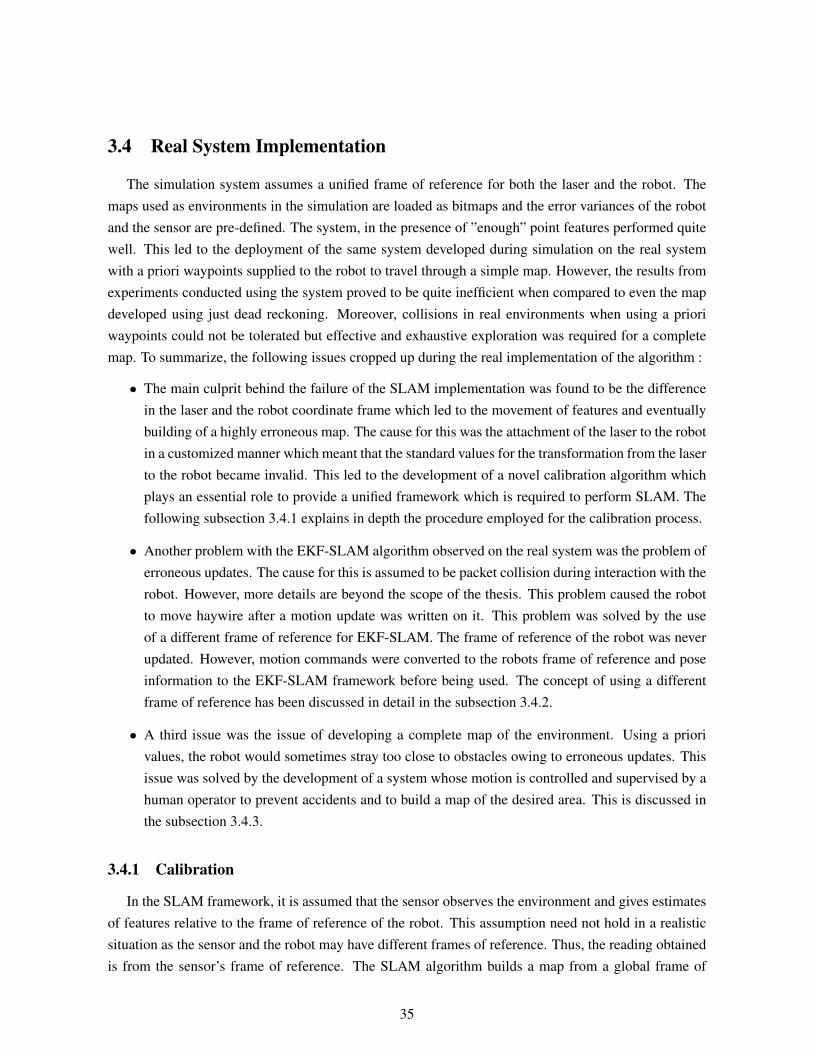
3.4 Real System Implementation

The simulation system assumes a unified frame of reference for both the laser and the robot. Themaps used as environments in the simulation are loaded as bitmaps and the error variances of the robotand the sensor are pre-defined. The system, in the presence of ”enough” point features performed quitewell. This led to the deployment of the same system developed during simulation on the real systemwith a priori waypoints supplied to the robot to travel through a simple map. However, the results fromexperiments conducted using the system proved to be quite inefficient when compared to even the mapdeveloped using just dead reckoning. Moreover, collisions in real environments when using a prioriwaypoints could not be tolerated but effective and exhaustive exploration was required for a completemap. To summarize, the following issues cropped up during the real implementation of the algorithm :

• The main culprit behind the failure of the SLAM implementation was found to be the differencein the laser and the robot coordinate frame which led to the movement of features and eventuallybuilding of a highly erroneous map. The cause for this was the attachment of the laser to the robotin a customized manner which meant that the standard values for the transformation from the laserto the robot became invalid. This led to the development of a novel calibration algorithm whichplays an essential role to provide a unified framework which is required to perform SLAM. Thefollowing subsection 3.4.1 explains in depth the procedure employed for the calibration process.

• Another problem with the EKF-SLAM algorithm observed on the real system was the problem oferroneous updates. The cause for this is assumed to be packet collision during interaction with therobot. However, more details are beyond the scope of the thesis. This problem caused the robotto move haywire after a motion update was written on it. This problem was solved by the useof a different frame of reference for EKF-SLAM. The frame of reference of the robot was neverupdated. However, motion commands were converted to the robots frame of reference and poseinformation to the EKF-SLAM framework before being used. The concept of using a differentframe of reference has been discussed in detail in the subsection 3.4.2.

• A third issue was the issue of developing a complete map of the environment. Using a priorivalues, the robot would sometimes stray too close to obstacles owing to erroneous updates. Thisissue was solved by the development of a system whose motion is controlled and supervised by ahuman operator to prevent accidents and to build a map of the desired area. This is discussed inthe subsection 3.4.3.

3.4.1 Calibration

In the SLAM framework, it is assumed that the sensor observes the environment and gives estimatesof features relative to the frame of reference of the robot. This assumption need not hold in a realisticsituation as the sensor and the robot may have different frames of reference. Thus, the reading obtainedis from the sensor’s frame of reference. The SLAM algorithm builds a map from a global frame of

35

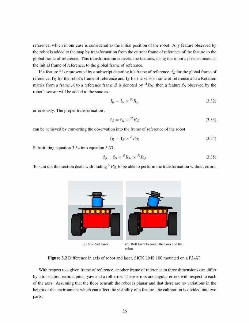
reference, which in our case is considered as the initial position of the robot. Any feature observed bythe robot is added to the map by transformation from the current frame of reference of the feature to theglobal frame of reference. This transformation converts the features, using the robot’s pose estimate asthe initial frame of reference, to the global frame of reference.

If a feature f is represented by a subscript denoting it’s frame of reference, fG for the global frame ofreference, fR for the robot’s frame of reference and fS for the sensor frame of reference and a Rotationmatrix from a frame A to a reference frame B is denoted by ARB, then a feature fS observed by therobot’s sensor will be added to the state as :

fG = fS × RRG (3.32)

erroneously. The proper transformation :

fG = fR × RRG (3.33)

can be achieved by converting the observation into the frame of reference of the robot.

fR = fS × SRR (3.34)

Substituting equation 3.34 into equation 3.33,

fG = fS × SRR × RRG (3.35)

To sum up, this section deals with finding SRR to be able to perform the transformation without errors.

(a) No Roll Error (b) Roll Error between the laser and therobot

Figure 3.2 Difference in axis of robot and laser, SICK LMS 100 mounted on a P3-AT

With respect to a given frame of reference, another frame of reference in three dimensions can differby a translation error, a pitch, yaw and a roll error. These errors are angular errors with respect to eachof the axes. Assuming that the floor beneath the robot is planar and that there are no variations in theheight of the environment which can affect the visibility of a feature, the calibration is divided into twoparts:

36

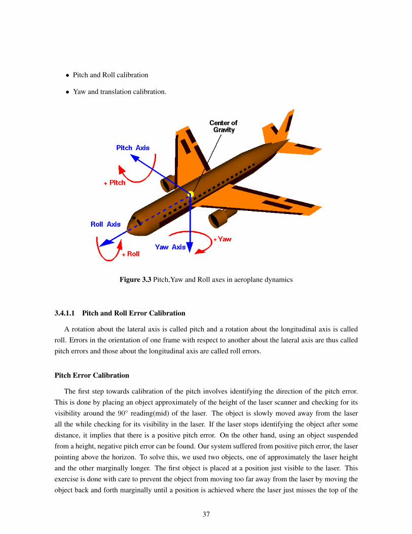
• Pitch and Roll calibration

• Yaw and translation calibration.

Figure 3.3 Pitch,Yaw and Roll axes in aeroplane dynamics

3.4.1.1 Pitch and Roll Error Calibration

A rotation about the lateral axis is called pitch and a rotation about the longitudinal axis is calledroll. Errors in the orientation of one frame with respect to another about the lateral axis are thus calledpitch errors and those about the longitudinal axis are called roll errors.

Pitch Error Calibration

The first step towards calibration of the pitch involves identifying the direction of the pitch error.This is done by placing an object approximately of the height of the laser scanner and checking for itsvisibility around the 90◦ reading(mid) of the laser. The object is slowly moved away from the laserall the while checking for its visibility in the laser. If the laser stops identifying the object after somedistance, it implies that there is a positive pitch error. On the other hand, using an object suspendedfrom a height, negative pitch error can be found. Our system suffered from positive pitch error, the laserpointing above the horizon. To solve this, we used two objects, one of approximately the laser heightand the other marginally longer. The first object is placed at a position just visible to the laser. Thisexercise is done with care to prevent the object from moving too far away from the laser by moving theobject back and forth marginally until a position is achieved where the laser just misses the top of the

37

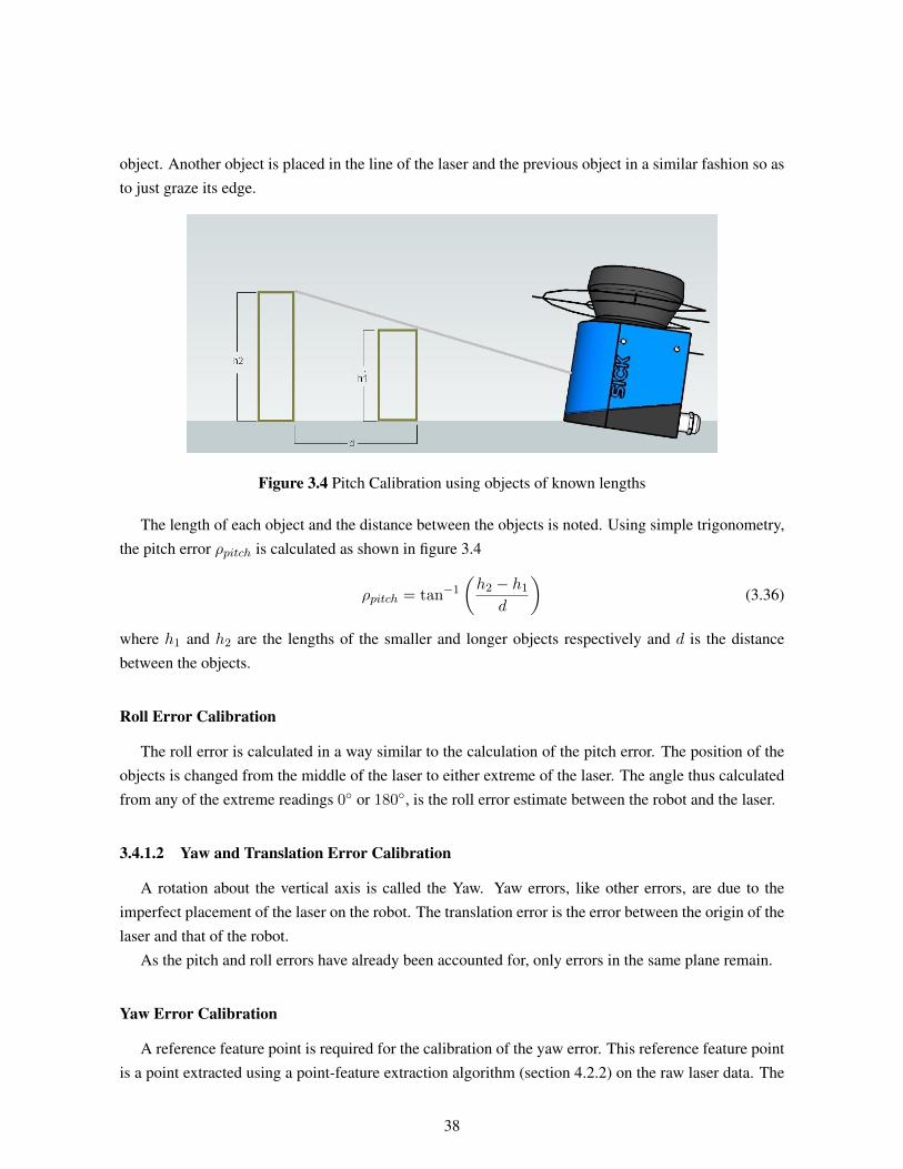
object. Another object is placed in the line of the laser and the previous object in a similar fashion so asto just graze its edge.

Figure 3.4 Pitch Calibration using objects of known lengths

The length of each object and the distance between the objects is noted. Using simple trigonometry,the pitch error ρpitch is calculated as shown in figure 3.4

ρpitch = tan−1

(h2 − h1

d

)(3.36)

where h1 and h2 are the lengths of the smaller and longer objects respectively and d is the distancebetween the objects.

Roll Error Calibration

The roll error is calculated in a way similar to the calculation of the pitch error. The position of theobjects is changed from the middle of the laser to either extreme of the laser. The angle thus calculatedfrom any of the extreme readings 0◦ or 180◦, is the roll error estimate between the robot and the laser.

3.4.1.2 Yaw and Translation Error Calibration

A rotation about the vertical axis is called the Yaw. Yaw errors, like other errors, are due to theimperfect placement of the laser on the robot. The translation error is the error between the origin of thelaser and that of the robot.

As the pitch and roll errors have already been accounted for, only errors in the same plane remain.

Yaw Error Calibration

A reference feature point is required for the calibration of the yaw error. This reference feature pointis a point extracted using a point-feature extraction algorithm (section 4.2.2) on the raw laser data. The

38

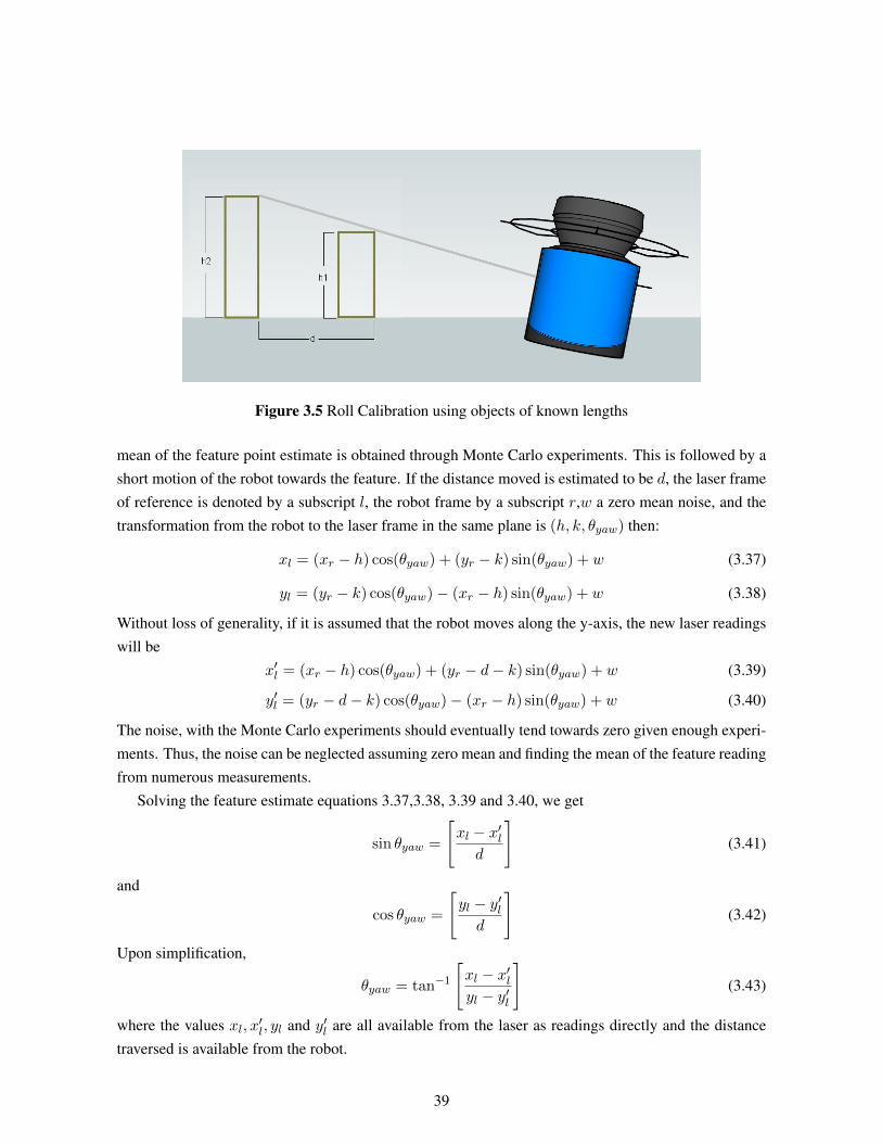
Figure 3.5 Roll Calibration using objects of known lengths

mean of the feature point estimate is obtained through Monte Carlo experiments. This is followed by ashort motion of the robot towards the feature. If the distance moved is estimated to be d, the laser frameof reference is denoted by a subscript l, the robot frame by a subscript r,w a zero mean noise, and thetransformation from the robot to the laser frame in the same plane is (h, k, θyaw) then:

xl = (xr − h) cos(θyaw) + (yr − k) sin(θyaw) + w (3.37)

yl = (yr − k) cos(θyaw)− (xr − h) sin(θyaw) + w (3.38)

Without loss of generality, if it is assumed that the robot moves along the y-axis, the new laser readingswill be

x′l = (xr − h) cos(θyaw) + (yr − d− k) sin(θyaw) + w (3.39)

y′l = (yr − d− k) cos(θyaw)− (xr − h) sin(θyaw) + w (3.40)

The noise, with the Monte Carlo experiments should eventually tend towards zero given enough experi-ments. Thus, the noise can be neglected assuming zero mean and finding the mean of the feature readingfrom numerous measurements.

Solving the feature estimate equations 3.37,3.38, 3.39 and 3.40, we get

sin θyaw =

[xl − x′ld

](3.41)

and

cos θyaw =

[yl − y′ld

](3.42)

Upon simplification,

θyaw = tan−1

[xl − x′lyl − y′l

](3.43)

where the values xl, x′l, yl and y′l are all available from the laser as readings directly and the distancetraversed is available from the robot.

39

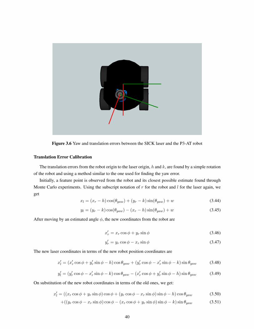
Figure 3.6 Yaw and translation errors between the SICK laser and the P3-AT robot

Translation Error Calibration

The translation errors from the robot origin to the laser origin, h and k, are found by a simple rotationof the robot and using a method similar to the one used for finding the yaw error.

Initially, a feature point is observed from the robot and its closest possible estimate found throughMonte Carlo experiments. Using the subscript notation of r for the robot and l for the laser again, weget

xl = (xr − h) cos(θyaw) + (yr − k) sin(θyaw) + w (3.44)

yl = (yr − k) cos(θyaw)− (xr − h) sin(θyaw) + w (3.45)

After moving by an estimated angle φ, the new coordinates from the robot are

x′r = xr cosφ+ yr sinφ (3.46)

y′r = yr cosφ− xr sinφ (3.47)

The new laser coordinates in terms of the new robot position coordinates are

x′l = (x′r cosφ+ y′r sinφ− h) cos θyaw + (y′r cosφ− x′r sinφ− k) sin θyaw (3.48)

y′l = (y′r cosφ− x′r sinφ− k) cos θyaw − (x′r cosφ+ y′r sinφ− h) sin θyaw (3.49)

On substitution of the new robot coordinates in terms of the old ones, we get:

x′l = ((xr cosφ+ yr sinφ) cosφ+ (yr cosφ− xr sinφ) sinφ− h) cos θyaw (3.50)

+((yr cosφ− xr sinφ) cosφ− (xr cosφ+ yr sinφ) sinφ− k) sin θyaw (3.51)

40

y′l = ((yr cosφ− xr sinφ) cosφ− (xr cosφ+ yr sinφ) sinφ− k) cos θyaw + w (3.52)

−((xr cosφ+ yr sinφ) cosφ+ (yr cosφ− xr sinφ) sinφ− h) sin θyaw + w (3.53)

On Simplification and assuming zero as the mean error and taking the mean values from Monte Carloexperiments,

x′l = xr cos(θyaw + φ) + yr sin(θyaw + φ)− h cos θ − k sin θ (3.54)

y′l = yr cos(θyaw + φ)− xr sin(θyaw + φ) + h sin θ − k cos θ (3.55)

Using the four equations 3.50, 3.52, 3.54 and 3.55, we are left with four unknowns the feature readingfrom the robot frame xr,yr,h and k. Solving these equations, we find the values h and k.

3.4.2 Independent Frame of reference

The EKF-SLAM algorithm updates the pose of the mobile robot every iteration. In our algorithm,this updated value needs to be written to the robot for it to know its updated position. However, it wasobserved that often the write operation to the robot would result in erroneous updating of the robot tothe global origin. This would cause an erroneous update in the robot pose and the resulting map wouldbe wayward. To prevent the issue of erroneous updates upon writing to the robot, the whole processof writing values to the robot was bypassed. Instead, the robot was never updated with the SLAMpose information and left in the odometry based pose estimate. This meant that two different framesof reference were to be maintained during the course of the EKF-SLAM algorithm. The odometrybased robot pose cannot be ignored as a move operation is executed on the real robot and accordingto its current position. Therefore, the move function was developed to identify the motion of the robotby querying the robot before and after the motion command is executed. The amount of motion iscalculated from the two robot poses and then supplied to the EKF-SLAM algorithm as the movement ofthe robot which is to be used by the prediction function in the algorithm.

3.4.3 Exploration

To prevent the development of only primitive maps based on simple a priori waypoints, a humanoperator supervised exploration has been attached to the system to be able to move accurately into allthe desired areas. The EKF-SLAM algorithm is paused at the beginning of each iteration. The robotis controlled using a joystick or the computer keyboard and a movement instruction is executed withthe EKF-SLAM algorithm. Upon termination of the movement, the EKF-SLAM algorithm is made tounpause and continue. Upon continuation, the EKF-SLAM algorithm queries for the new pose of therobot, finds the movement and then the prediction stage of the algorithm is executed.

3.4.4 Online and Offline Versions

Two versions of the EKF-SLAM system have been deployed as part of this work:

41

• Online SLAM

• Offline SLAM

3.4.4.1 Online SLAM

The online SLAM version is not to be confused with the online SLAM problem which deals withestimating the current robot pose while estimating the map and is different from the full SLAM problem.The online SLAM version is a deployment with the ability to build maps on-the-fly. This system canbe given exploration based control inputs to be able to build a map while localizing in it to preventcollisions. This version of SLAM is given two kinds of control inputs to build a map.

The first kind of control input is a predefined set of waypoints for the path of the robot. This is givenon the basis of an estimated path whose possibility is pre-evaluated manually. This version of SLAM iscompletely autonomous and requires no user intervention after the system has been initialized.

The second kind of control input is an active user control input which is used to create maps that needto be as complete as possible. The input is given during the course of each iteration when the SLAMalgorithm is paused as the robot executes a control command. Upon completion of the execution, theSLAM iteration is resumed and completed and pauses again for a control input. This process ensures thatthe user can steer the robot as he/she desires and can develop a map of all areas by manually employingthe exploration. It is to be noted that the control input is taken as the difference between the robot posebefore and after the execution of the robot movement through the use of steering instrument(keyboard,joystick). This implies that each control input can only be a translation or a rotation.

The principal advantage of an online SLAM system is autonomous execution when used with anexploration algorithm.

3.4.4.2 Offline SLAM

The offline SLAM version is much like the online SLAM algorithm except for one vital difference.The SLAM algorithm is not executed on the robot during the course of its exploration. The robot iseither manually or through the use of predefined waypoints made to sense the environment. Duringthe course of the movement of the robot, no SLAM algorithm is performed. Rather, the process ofrobot exploration is utilized to collect odometry and laser data. This information is stored in files as therobot keeps exploring. Upon the termination of exploration, the data stored by the on-board computeris then retrieved to perform EKF-SLAM offline. The utility of an offline SLAM is the ability to tweakparameters and check the performance of the algorithm with different versions. Moreover, an offlineSLAM ensures higher level of accuracy as data is collected at more than 9 Hz which ensures a largenumber of SLAM iterations before the map is built and hence also ensure a lower amount of error dueto multiple citing of features.

42

3.4.5 Complete Metric Map Building

The problem tackled in this work is called the online SLAM problem. The online SLAM problemmaintains only the current pose of the robot in the state vector along with features while all earlier robotstates are discarded. On the other hand, the full SLAM problem maintains all the robot poses in thestate too. The advantage of using a full SLAM algorithm is the availability of all updated robot poseestimates. This implies the availability of the trajectory traversed by the robot. This trajectory combinedwith laser readings from each pose estimate can be used to build a map by the re-projection of the laserhits from corrected robot poses, which will be called the complete metric map. A complete metric mapmay suffer from local observation error but the as the robot pose error is low, the global overhead of thefeature error is minimal. Thus a full SLAM solution is effective towards building a more informativemap. The complete metric map can be utilized by the robot for path planning, to be able to reach adestination from its position avoiding obstacles and finding the optimal route.

However, the catch is the complexity of the full SLAM algorithm. The state vector of the robot inthe online SLAM problem is

xk =

xv,k

xf1,k

.

.

.

xfn,k

(3.56)

where xv,k represents the robot pose estimate at time instant k. On the other hand, the state vector inthe full SLAM problem is

xk =

xv,1

.

.

.

xv,k

xf1,k

.

.

.

xfn,k

(3.57)

Clearly, the state vector for the full SLAM problem increases not only with every feature added but alsowith each iteration of the algorithm as it adds all robot pose estimates into the state.

After t iterations of the algorithm, an online SLAM state vector will have the size nv +knf if nv arethe dimensions of the robot pose and nf are the dimensions of the feature pose and there are k featuresin the state. In a full SLAM system, the state vector will be of the size tnv +knf after t iterations of the

43

algorithm. The corresponding covariance matrices will be of the dimensions (nv + knf )× (nv + knf )

and (tnv + knf ) × (tnv + knf ) for online and full SLAM respectively. The computational cost ofupdating the state of the SLAM system in the online case is hence O((nv + knf )2) and in the fullSLAM case, O((tnv + knf )2).

A practical assumption that the number of features are greater than the dimensions of the robot poseand the feature estimate

k � nf and k � nv (3.58)

gives a computational complexity of O(k2) in the online SLAM case.In the full SLAM case, we have two variables t, the number of iterations, and k, the number of

features. Generally, the number of iterations are performed as many times as possible to increase theobservations, associations and therefore, keep the errors in check. In other words,

t� k (3.59)

Thus, the computational complexity of a SLAM update after t iterations in the full SLAM case is O(t2)

which is greater than the complexity of the online SLAM version. Thus the advantage of the full SLAMsolution of finding the trajectory comes at the cost of a greater computational complexity.

Instead of using a full SLAM solution, we solve the problem of improving robot pose estimates atall times instants using a EKF-smoother.

3.4.5.1 Smoothing

The Kalman smoothing process is an offline process applied after the termination of the EKF-SLAMalgorithm. The smoothing process improves the earlier estimate of the state by using the later estimateas an observation. The smoothing process is running the EKF filter backwards from the last updatedrobot state to the initial robot state, each time using the next updated robot state in time as an observationfor correction of the robot state at the considered time instant. Similar to the EKF-SLAM algorithm, thesmoothing process has two stages every iteration:

• Prediction Stage

• Update Stage

State transitionxk+1 = f(xk,uk,vk) (3.60)

Observation modelzk+1 = xk+1 (3.61)

The prediction stage involves predicting the next state of the system. In the smoother, we attempt tocorrect the pose of a robot at each time instant. Each iteration of the EKF-SLAM algorithm involves themovement of the robot, followed by a prediction and an update. Using the predicted values of the robot

44

as the predicted observation, the current pose is estimated through the smoother. In other words, insteadof estimating the robot state at time k + 1 given a position and a movement at time k, the smootherestimates the robot state at time k, given a prediction and an observation of the state at k + 1, which isalready smoothed.

In fact, values, if stored from the forward run of the EKF-SLAM algorithm, can be utilized directlyas prediction for smoothing

xk+1|k = f(xk|k,uk,0) (3.62)

P sk+1|k = FkPk|kF′k + TQkT

′ (3.63)

The predicted state value for the next iteration from the prediction stage in the smoothing process isnot the state to be corrected, rather it is used as the predicted observation model.

The updated(smoothed) estimate at time instant k is found using :

xsk|k = xk|k +K(xsk+1|k+1 − xk+1|k) (3.64)

where K, the kalman gain is

K =Pk|kF

′k

P sk+1|k(3.65)

P sk|k = (I −KFk)Pk|k (3.66)

This updated set of robot poses is used to plot all the laser data. Results obtained by the use of EKFsmoothing have aided in the construction of a better complete laser map. The smoothed results can beviewed in section 5.3.

3.5 Summary

This chapter discusses system specifics for the implementation of the EKF-SLAM algorithm on thePioneer P3-Dx robot using a laser range finder as the measurement sensor. Specifically, the motionmodel and sensor model parametrization has been discussed.

This is followed by the details of simulation based implementation using the developed models. Therest of the chapter deals with the implementation-specific paradigms which arose due to the constraintsassumed for the system. These include:

• The issue of handling data from different reference frames has been handled by a novel calibrationmethod of the laser with respect to the robot.

• Manual exploration based implementation and the provision of two different frames of references,one for odometry and another for SLAM has been summarized in the next subsection.

• Developing a SLAM algorithm version to function on-the-fly and another to work with datasets.

45

The last subsection in this chapter deals with the development of a complete metric map which includesnot only the feature map but a complete corrected scan map for the provision of path planning. Thisdevelopment process is performed offline after the termination of the EKF-SLAM algorithm using anEKF smoother.

46

Chapter 4

Features

Information extracted from raw laser that can be stored, estimated and be identified uniquely arecalled features. Features are parts of the environment that can be used by the mobile robot as landmarksto localize itself while it also updates the map. Depending upon the sensor that is used, the parametersof a feature can vary from simple distance from origin in a 1-dimensional environment to a completegeometry of the visible structure with color information. In our context, a laser scanner is used tosense the environment. The laser gives data pertaining to a 2-dimensional slice of the 3-dimensionalenvironment with distances of obstacles from the laser.

The raw information provided by the laser provides us a top-view like understanding of the environ-ment. Clearly, only geometrical features can be extracted from such information. Feature points can beused as primitive geometric features that can be uniquely determined from the laser data. These uniquepoint features can be features that are formed by the intersection of two line-segment objects or by theedge of a line-segment object. These feature points are stored in the state vector in the form of theircoordinates in the estimated global framework of the robot. For matching these point features, we usean association algorithm that determines whether the current observation is one of an earlier observedfeatures based on a nearness metric.

The following section of this chapter explains the process used to extract features for the SLAMalgorithm, which is followed by an algorithm used to associate observations to features in the statevector. The next subsections deal with problems of identifying features and working in environmentswith scarce features.

4.1 Types of Features

A laser scan provides information of a plane cut with the laser range as the maximum distancepossible in a semi-circular scan. This scan resembles a top-view of the environment. Upon simpleintrospection, it is observed that geometry based features are the only possibility to be used throughlaser. Numerous kinds of features can be extracted from the laser data according to the parametrizationplanned for the EKF-SLAM algorithm. However, the most used and most reliable features for robust

47

deployment remain point based features. In this work, we have used three different feature parametriza-tions:

• Point features

• Line features

• MECP features

Line features are line segments extracted from the laser scan. Point features are corners and edgesof the line segments of objects extracted from the laser scan. The MECP features are a combination ofselected point features using some geometric information about their surroundings which make themeasily recognizable in future iterations.

4.2 Point Features

Point features are the most common type of features used for building a range scanner based featuremap. The range scanner is assumed to follow a Gaussian error distribution. That is, the angle and therange value have a mean and an error variance which they are assumed to follow. A point feature is oneof the selected range information obtained whose error, by the aforementioned assumption implicitlyfollows a normal distribution.

Hence, the use of point features is the most deployed kind of EKF-SLAM in literature.

4.2.1 Parametrization of Point Features

Any point feature observed by the range finder can be expressed as

zk =

[rk

θk

](4.1)

where rk is the range reading obtained for the angle θk. The point features thus considered can beconsidered to have Gaussian errors only in their (rk, θk) frame only. The estimate of these points islinearized in the EKF-SLAM algorithm to find the variance in the global framework of the SLAM forthe purpose of augmenting the features.

The observation model can be written as

zfk =

√(xv − xfk)2 + (yv − yfk)2

tan−1(yv−yfkxv−xfk

)− θv

(4.2)

48

4.2.2 Point Feature Extraction

Point Features are extracted from the raw laser scan by a data extraction algorithm. The data extrac-tion function can be divided into two parts:

• Data Clustering

• Split-and-Merge Line Division

Each part of the extraction process are explained in detail in the subsections below.

4.2.2.1 Data Clustering

Data Clustering is the division of data based on its identification with a certain part of the environ-ment. Data clustering partitions the given data into smaller sets where each set is assumed to belong toan object in the environment. The clustering of data ensures that only continuous data points are utilizedto form lines and eventually points.

The data clustering implemented in this work consists of clustering of points based on their mutualdistance. This method traverses through the range data in the order of the angles from which it wasobtained. If the resolution of the laser is 1 deg, and rθ is the reading at angle θ, and rθ+1, the readingfrom the next angle θ + 1, then the euclidean distance between the two observed points is√

(rθ+1 cos(θ + 1)− rθ cos(θ))2 + (rθ+1 sin(θ + 1)− rθ sin(θ))2 (4.3)

A threshold hc is defined a priori to the algorithm. All consecutive points with mutual distances lessthan the threshold are then put into the same cluster. A mutual distance greater than the threshold beginsa new cluster where consecutive points are added till the mutual distance is found to be greater than thethreshold level.

The threshold value hc, which is to be fed a priori, has a huge impact on the accuracy and granularityof the clustering. A threshold too large will end up labelling numerous objects which are not far apartas the same object and one too small will end up dividing a single object further. The apt value for h isdependent on the structure of the environment and cannot be generalized for all environments. The valueof hc for different maps in this work has been calculated through Monte Carlo experiments according toeach environment of implementation.

4.2.2.2 Split-and-Merge Line Division

Data from each partition formed by the clustering process is broken into a point set using the Split-and-Merge algorithm, consecutive points representing one line. Each partition of data, which is again, aset of points with consecutive angular readings, is then reduced to sets of points that define the structureof the object and thus can be distinguished with ease from other points nearby.

49

The Douglas-Peucker algorithm is used to find the lines that form an object from a cluster. Alsoknown as the split-and-merge algorithm, it is a recursive algorithm to identify key points from a givenset. the Douglas-Peucker algorithm is explained in brief below:

The input to the algorithm is an ordered set of points and a distance threshold hf . The algorithmrecursively divides the set into lines. The first and last points are automatically chosen to be kept.The algorithm first draws a line segment between the first and the last points. It then finds the pointthat is farthest from the line segment. If the point is closer than the threshold given, hf , to the linesegment, then all the data points between these two endpoints are discarded. If the point farthest fromthe line segment is greater than the threshold hf then that point is added to the output set. The algorithmrecursively calls itself with the first point and the farthest point and then with the farthest point and thelast point until no points between all the line segments with a distance greater than the threshold, areleft. When the recursion is completed, a new output point set is generated consisting of all the pointsthat have not been discarded. These points are the points of interest to be used as observations in thealgorithm.

4.2.3 Point Feature Association

Feature Association is arguably the most important part of the SLAM algorithm. The correct corre-spondence of an observed feature with one in the state vector is essential for the building a consistentmap. Incorrect feature association is a common hurdle to build a reliable map and a single wrongassociation can lead to a failure in efficient map building.

Feature association maps observed information in the current iteration which is obtained relative tothe pose of the robot to a feature observed in earlier iterations and stored in the state vector. Featureassociation depends heavily on the error in the robot, the higher the error in the robot pose, the tougher itbecomes to associate features. As we use a laser based sensor for environment observation, the features,which are extracted from the range data, can only be distinguished by their locations. Moreover, sincewe use a Gaussian representation for all the features, the pdf spreads from−∞ to∞, making it possiblefor association between any feature and any observation. However, to accept only associations that arelikely, only features in the vicinity of the observation are to be considered.

Features are associated using a validation gate which defines the maximum permissible error betweenthe observation and the expected observation. A validation gate based on the Mahalanobis distance hasbeen used for feature association in this work. For an observation zi and an expected observation zk,for a feature xfk , where zk = h(xfk), the innovation is defined as

vik = zi − zk (4.4)

The Mahalanobis distance, also known as the Normalised Innovation Squared(NIS) is defined as

Mik = vikS−1ik v

′ik (4.5)

50

where the innovation variance, SikSik = HkPHk +Ri (4.6)

For a Gaussian distributed innovation sequence, the Mahalanobis distance forms a χ2 distributionwhose shape is dependent on the dimensions of the innovation vector, vik. Validation of a match ishence performed by checking for a maximum Normalized Innovation squared(NIS) thresholdMik < ηn

where n is the dimension of the innovation sequence and hence of the χ2 distribution.

This validation can be understood as an ellipsoid in the frame of the robot, centred about the predictedobservation. Thus, for an observation to be matched with the feature, it needs to fall within the ellipse.However, multiple observations might fall within the ellipse. To resolve the ambiguity in association,there is a need to select the observation closest to the feature by some metric. In this work, a nearestneighbour based feature association is used to handle ambiguity.

For a set of observations z = {z1, · · · , zn} seen in the same time instant, the likelihood associationfor each feature zi with thekth feature in the state vector can be calculated as

Ai =1

(2π)n/2√|Sik|

e−12vi′Sik

−1vi (4.7)

The normalized distance Ni, which is an equivalent metric is obtained by taking logs of equation 4.7

Ni = vi′Sik

−1vi + ln|Sik| (4.8)

The nearest neighbour feature association algorithm, given an observation zi chooses that feature kfrom the state which minimizes the value of Ai is chosen as the matching feature for the given observa-tion.

However, in cases where there are no features that obey the validation gate for a certain observation,then the observation is considered a unique feature and is augmented to the state after then update stage.

The nearest neighbour feature association algorithm selects that feature from the state as the matchfor the observation which minimizes the value of Ni . This feature association is performed for eachobservation from the range scanner against all features in the state vector.

4.2.4 Point Feature Augmentation

As the environment is explored, new features observed in each iteration are added to the robot stateand the corresponding values are to be filled in the covariance matrix to be able to track and match thesefeatures. The polar values of the observation zi, which are in polar coordinates ri and θi are added tothe state by converting them into Cartesian coordinates with respect to the global frame of the SLAMsystem. A function a(xk, zi) is used to convert the values into the Cartesian system:

a(x, zi) =

[xf i

yf i

]=

[xv,k + ri cos(θv,k + θi)

yv,k + ri sin(θv,k + θi)

](4.9)

51

The point being added to the state has Gaussian error in the polar coordinates. This has to be approx-imated to a Gaussian in the global Cartesian frame. This is accomplished by the use of a Taylor seriesfirst order approximation with a Jacobian of the function a.

The observation function can be written as

xfj = a(xk, zi) + af (wk) (4.10)

This function can be linearized at the estimated robot pose as

xfj ≈ a(xk, zi) +Av[xk − xk] +Af [wk] (4.11)

The covariance can be found as

E[[xfj − xfj ][xfj − xfj ]′] (4.12)

which can be simplified as

Pfj ,k = AvPv,kA′v +AfRiA

′f (4.13)

where

Av =

[1 0 −ri sin θi

0 1 ri cos θi

](4.14)

Af =

[cos θi −ri sin θi

sin θi ri cos θi

](4.15)

Similarly, the covariance added due to augmented feature can be calculated as

Pfj ,: = AvPvm (4.16)

and

P:,fj = PvmA′v (4.17)

where Pvm is the covariance of the robot pose with all features in the state vector present a prioriand Pfj ,: are the rows of the covariance matrix associated with the feature fj and P:,fj , the columns,respectively.

The new state after the augmentation process becomes:

x =

[x

xfj

](4.18)

and the new covariance becomes:

P =

Pvv Pvm PvvA′v

Pmv Pmm PmvA′v

AvPvv AvPvm AvPvvA′v +AfRiA

′f

(4.19)

52

4.3 Line based features

Although the point feature association algorithm performs efficiently in the presence of ample pointfeatures, mapping often fails when the number of features are few and far. This is attributed to the factthat low feature density causes a low variance reduction and may lead to the build up of error variancein the robot. A high error variance in the robot pose causes ambiguity in association and may hamperthe building of a reliable map.

Thus, the visibility of features can be seen as an important requirement for the EKF-SLAM to func-tion as expected. However, for parts of map which resemble empty corridors, which are long areas withno or few corners, the data association algorithm fails to associate accurately if the robot variance isvery high.

Hence, it is essential to always keep the robot pose variance as low as possible to be able to builda consistent map. This requirement led to the development of using lines as features so that the vari-ance of the robot does not increase without bounds which would benefit point feature association andconsequently enable the construction of an efficient map.

In this section, the concern is about approaches that use both point and segment features as land-marks. The amount of literature on line segment based EKF SLAM has been relatively sparse. In arecent paper [25], a line feature based SLAM with lower end sensors such as an IR range finder wasproposed. The paper formulates the framework for segments that are parallel to one of the two axesof the global reference frame. In Connette’s work [26], the line feature is represented by its center ofgravity. By tracking corners that form the endpoints of the line the statistical growth of line like featuresis curtailed. Earlier, a framework of SLAM based on segment representation and map management waspresented by Garulli [21]. However this work did not consider incorporating point features also as partof the landmarks.

EKF-SLAM based on orthogonal line features only or point features only has been explored inliterature. However,to our knowledge, an EKF-SLAM implementation considering both point and linefeatures has not been researched on in the robotics literature. The reason for including line features istheir visibility even in environments where point features might be sparse. The robot pose error varianceneeds to be bounded. Otherwise, it renders feature association inefficient and thus an inaccurate map isthe result. The main cause for the growth in the error variance of the robot pose is the robot movement atthe beginning of each iteration of the EKF-SLAM algorithm. This growth is countered by a reduction inthe variance in the update stage of SLAM. However, if there are no features visible, the update stage doesnot alter any part of the state or the matrix. Thus, if features are not visible for numerous successiveiterations, the robot pose error variance becomes too high to be even able to associate subsequentlyvisible features. If the robot pose covariance at the time step k is Pv,k

Pv,k =

pxx pxy pxθ

pyx pyy pyθ

pθx pyθ pθθ

(4.20)

53

After the prediction stage, the covariance becomes

Pv,k+1|k = Gv

pxx pxy pxθ

pyx pyy pyθ

pθx pyθ pθθ

G′v

+GuRkG′u (4.21)

where

Gv =

1 0 −r sin θv

0 1 r cos θv

0 0 1

(4.22)

On simplification and substituting a = −r sin θv and b = r cos θv,

Pv,k+1|k =

pxx + 2apxθ + a2pθθ pxy + apyθ + bpxθ + abpθθ pxθ + apθθ

pxy + bpxθ + apyθ + abpθθ pyy + 2bpyθ + b2pθθ pyθ + bpθθ

pxθ + apθθ pyθ + bpθθ, pθθ

+GuRkG′u

(4.23)Thus, there is a huge impact of the variance in θ in the robot pose variance. The value, pθθ increasesupon each rotation. Therefore, the robot heading error is the primary reason for a high variance effecton the robot variance. To be able to build a consistent map, one should attempt to keep the heading erroras small as possible.

4.3.1 Parametrization of Line based features

Often, it was observed during our experiments that line features are visible even in environmentswhere point features are seldom visible. This incentive led to the use of line based features for SLAM.Our parametrization for line based features is based on the normal form of the line:

x cos θ + y sin θ = p (4.24)

where θ is the angle of inclination with the x-axis and p is the length of the perpendicular from origin.This formulation always has finite values for the parameters θ and p for all visible line features whichmakes it usable in all circumstances. The line feature is stored in the states using the two aforementionedparameters as

xfk =

[pfkθfk

](4.25)

This formulation leads to the following observation model

z =

[xv,x cos θfk + xv,y sin θfk − pfk

θfk − xv,θ

](4.26)

where xv,x, xv,y and θfk are the estimates for the x-coordinate,y-coordinate and the heading of the robotpose estimate respectively.

54

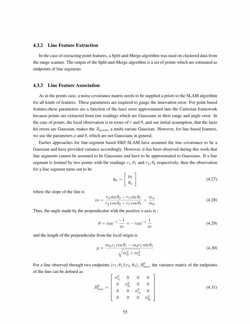
4.3.2 Line Feature Extraction

In the case of extracting point features, a Split-and-Merge algorithm was used on clustered data fromthe range scanner. The output of the Split-and-Merge algorithm is a set of points which are estimated asendpoints of line segments.

4.3.3 Line Feature Association

As in the points case, a noise covariance matrix needs to be supplied a priori to the SLAM algorithmfor all kinds of features. These parameters are required to gauge the innovation error. For point basedfeatures,these parameters are a function of the laser error approximated into the Cartesian frameworkbecause points are extracted from raw readings which are Gaussians in their range and angle error. Inthe case of points, the local observation is in terms of r and θ, and our initial assumption, that the laserhit errors are Gaussian, makes the Rpoints a multi-variate Gaussian. However, for line based features,we use the parameters p and θ, which are not Gaussians in general.

Earlier approaches for line-segment based EKF-SLAM have assumed the line covariance to be aGaussian and have provided variance accordingly. However, it has been observed during this work thatline segments cannot be assumed to be Gaussians and have to be approximated to Gaussians. If a linesegment is formed by two points with the readings r1, θ1 and r2, θ2 respectively, then the observationfor a line segment turns out to be

zk =

[pk

θk

](4.27)

where the slope of the line is

m =r2 sin θ2 − r1 sin θ1

r2 cos θ2 − r1 cos θ1=mn

md(4.28)

Thus, the angle made by the perpendicular with the positive x-axis is :

θ = tan−1 −1

m= − tan−1 1

m(4.29)

and the length of the perpendicular from the local origin is

p =mnr1 cos θ1 −mdr1 sin θ1√

m2n +m2

d

(4.30)

For a line observed through two endpoints (r1, θ1)(r2, θ2), Rpline, the variance matrix of the endpointsof the line can be defined as

Rpline =

σ2r1 0 0 0

0 σ2θ1

0 0

0 0 σ2r2 0

0 0 0 σ2θ2

(4.31)

55

This has to be approximated to a Gaussian in the pk and θk frame. The Jacobian can be calculated by

T =

∂pk∂r1

∂pk∂θ1

∂pk∂r2

∂pk∂θ2

∂θk∂r1

∂θk∂θ1

∂θk∂rθ2

∂θk∂θ2

(4.32)

where

pk =r1r2 sin(θ2 − θ1)

r21 + r2

2 − r1r2 cos(θ1 − θ2)(4.33)

and

θk = −tan−1

[r2 cos θ2 − r1 cos θ1

r2 sin θ2 − r1 sin θ1

](4.34)

Thus, the variance Rlines can be written in the reference frame of the line parametrization throughthe approximation TRplinesT

′.However, through the course of numerous runs in different simulated environments, it was observed

that the approximation did not hold good for the p value and often lead to overconfident assumptions ofthe filter and an inconsistent map. This was primarily because the approximated variance would oftenturn out to be an underestimation. These results were discernible only after experiments with long runsin simulated environments. The longer the robot travelled, the greater the inconsistency of the map asthe approximated variance often proved to be an unacceptable one.

The value pfk was therefore omitted from the line feature parametrization and line features repre-sented as θfk . The issue with this representation is the issue of feature association. Near parallel lineshave the same θfk and hence can be matched to each other. However, the actual line might be differentand we need the other parameter, the perpendicular distance, to match the line feature. This perpendicu-lar distance is extracted from the end points of line features which are stored as point features wheneveratleast one endpoint has been added to the state. This leads to two cases of line feature association:

• One Endpoint in State

• Both Endpoints in State

One Endpoint in State

If only one endpoint of the line has been seen till the current iteration, we consider the predictedobservation using the end point and the line feature estimate from the state. This is calculated as:

zk =

[xv sin θk − yv cos θk − xf sin θk + yf cos θk

θk − θv

],

[n1

n2

](4.35)

The corresponding Jacobian can be derived as

H =

∂n1∂xv

∂n1∂yv

∂n1∂θv

· · · ∂n1∂xf

∂n1∂yf

· · · ∂n1∂θfk

· · ·∂n2∂xv

∂n2∂yv

∂n2∂θv

· · · ∂n2∂xf

∂n2∂yf

· · · ∂n2∂θfk

· · ·

(4.36)

56

which can be simplified as

H =

[sin θk − cos θk 0 · · · − sin θk cos θk · · · −xf cos θk − yf sin θk · · ·

0 0 −1 · · · 0 0 · · · 1 · · ·

](4.37)

Association of a visible line from the sensor information is performed using the same Mahalanobisdistance from the innovation, v and the innovation variance, S.

Both Endpoints in State

For each line segment which has both endpoints in the state, the predicted observation can be calcu-lated as

zlines =

xv(yf1−yf2 )+yv(xf2−xf1 )√(xf2−xf1 )2+(yf2−yf1 )2

θfk − θv

,

[n1

n2

](4.38)

The corresponding Jacobian can be derived as

H =

∂n1∂xv

∂n1∂yv

∂n1∂θv

· · · ∂n1∂xf1

∂n1∂yf1

· · · ∂n1∂xf2

∂n1∂yf2

· · · ∂n1∂θline1

· · ·∂n2∂xv

∂n2∂yv

∂n2∂θv

· · · ∂n2∂xf1

∂n2∂yf1

· · · ∂n2∂xf2

∂n2∂yf2

· · · ∂n2∂θline1

· · ·

(4.39)

which simplifies to

H =

yf1−yf2d

xf2−xf1d 0 · · · −yvn1 xvn2 · · · yvn1 xvn2 · · · 0 · · ·

0 0 −1 · · · 0 0 · · · 0 0 · · · 1 · · ·

(4.40)

where

d =√

(xf2 − xf1)2 + (yf2 − yf1)2 (4.41)

n1 =d2 + 3(xf2 − xf1)2

d3(4.42)

and

n2 =d2 + 3(yf2 − yf1)2

d3(4.43)

Line feature association is performed in a fashion similar to the point feature association(in section4.2.3) using a Mahalanobis distance based association as we have both v, the innovation and S, theinnovation covariance.

4.3.4 Line Feature Augmentation

Line features are added as the angle subtended by the perpendicular to the line from the origin withthe positive x-axis. The feature is stored as

θfk = θk + θv (4.44)

57

Pfk = Pθv + TRplineT′ (4.45)

whereT =

[∂θk∂r1

∂θk∂θ1

∂θk∂rθ2

∂θk∂θ2

](4.46)

Similarly, the covariance added due to augmented feature can be calculated as

Pfk,: = Pθvm (4.47)

where Pθvm is the covariance of the robot heading with all features in the state vector present a priori.

4.3.5 Results

Inconsistent maps upon the use of point only SLAM led to the use of line and points as features whileomitting the perpendicular distance p, as it was observed to improve the mapping. The below resultsare from a simulated run in playerstage showing the performance of SLAM when lines are also used asfeatures.

Figure 4.1 EKF-SLAM trailsThe blue line: Actual path to be followed by the robot. The red trail: Actual path taken by the robot

using point features SLAM. The green trail: Actual path taken when both points and lines(θ only) areused. Black lines: The map

58

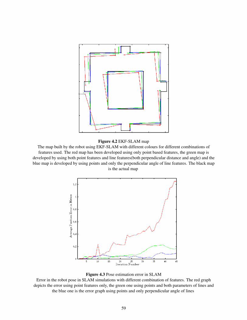
Figure 4.2 EKF-SLAM mapThe map built by the robot using EKF-SLAM with different colours for different combinations offeatures used. The red map has been developed using only point based features, the green map is

developed by using both point features and line features(both perpendicular distance and angle) and theblue map is developed by using points and only the perpendicular angle of line features. The black map

is the actual map

Figure 4.3 Pose estimation error in SLAMError in the robot pose in SLAM simulations with different combination of features. The red graph

depicts the error using point features only, the green one using points and both parameters of lines andthe blue one is the error graph using points and only perpendicular angle of lines

59

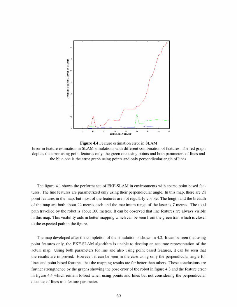
Figure 4.4 Feature estimation error in SLAMError in feature estimation in SLAM simulations with different combination of features. The red graphdepicts the error using point features only, the green one using points and both parameters of lines and

the blue one is the error graph using points and only perpendicular angle of lines

The figure 4.1 shows the performance of EKF-SLAM in environments with sparse point based fea-tures. The line features are parametrized only using their perpendicular angle. In this map, there are 24

point features in the map, but most of the features are not regularly visible. The length and the breadthof the map are both about 22 metres each and the maximum range of the laser is 7 metres. The totalpath travelled by the robot is about 100 metres. It can be observed that line features are always visiblein this map. This visibility aids in better mapping which can be seen from the green trail which is closerto the expected path in the figure.

The map developed after the completion of the simulation is shown in 4.2. It can be seen that usingpoint features only, the EKF-SLAM algorithm is unable to develop an accurate representation of theactual map. Using both parameters for line and also using point based features, it can be seen thatthe results are improved. However, it can be seen in the case using only the perpendicular angle forlines and point based features, that the mapping results are far better than others. These conclusions arefurther strengthened by the graphs showing the pose error of the robot in figure 4.3 and the feature errorin figure 4.4 which remain lowest when using points and lines but not considering the perpendiculardistance of lines as a feature paramater.

60

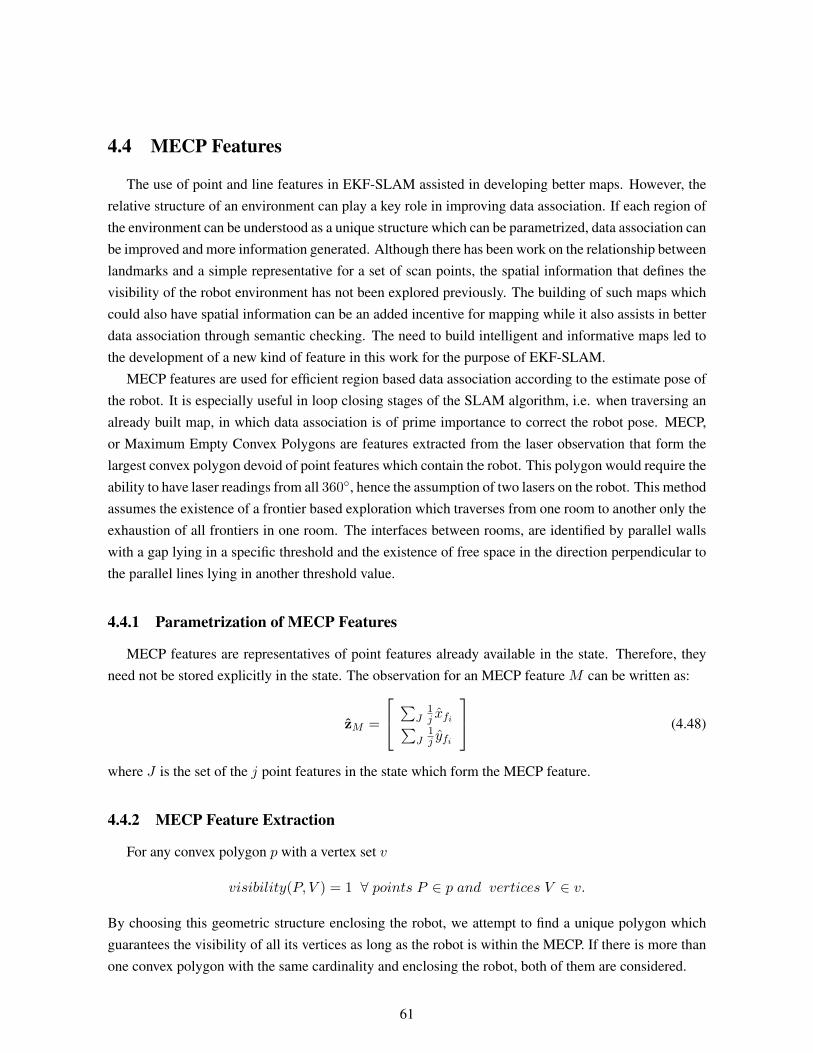
4.4 MECP Features

The use of point and line features in EKF-SLAM assisted in developing better maps. However, therelative structure of an environment can play a key role in improving data association. If each region ofthe environment can be understood as a unique structure which can be parametrized, data association canbe improved and more information generated. Although there has been work on the relationship betweenlandmarks and a simple representative for a set of scan points, the spatial information that defines thevisibility of the robot environment has not been explored previously. The building of such maps whichcould also have spatial information can be an added incentive for mapping while it also assists in betterdata association through semantic checking. The need to build intelligent and informative maps led tothe development of a new kind of feature in this work for the purpose of EKF-SLAM.

MECP features are used for efficient region based data association according to the estimate pose ofthe robot. It is especially useful in loop closing stages of the SLAM algorithm, i.e. when traversing analready built map, in which data association is of prime importance to correct the robot pose. MECP,or Maximum Empty Convex Polygons are features extracted from the laser observation that form thelargest convex polygon devoid of point features which contain the robot. This polygon would require theability to have laser readings from all 360◦, hence the assumption of two lasers on the robot. This methodassumes the existence of a frontier based exploration which traverses from one room to another only theexhaustion of all frontiers in one room. The interfaces between rooms, are identified by parallel wallswith a gap lying in a specific threshold and the existence of free space in the direction perpendicular tothe parallel lines lying in another threshold value.

4.4.1 Parametrization of MECP Features

MECP features are representatives of point features already available in the state. Therefore, theyneed not be stored explicitly in the state. The observation for an MECP feature M can be written as:

zM =

∑J1j xfi∑

J1j yfi

(4.48)

where J is the set of the j point features in the state which form the MECP feature.

4.4.2 MECP Feature Extraction

For any convex polygon p with a vertex set v

visibility(P, V ) = 1 ∀ points P ∈ p and vertices V ∈ v.

By choosing this geometric structure enclosing the robot, we attempt to find a unique polygon whichguarantees the visibility of all its vertices as long as the robot is within the MECP. If there is more thanone convex polygon with the same cardinality and enclosing the robot, both of them are considered.

61

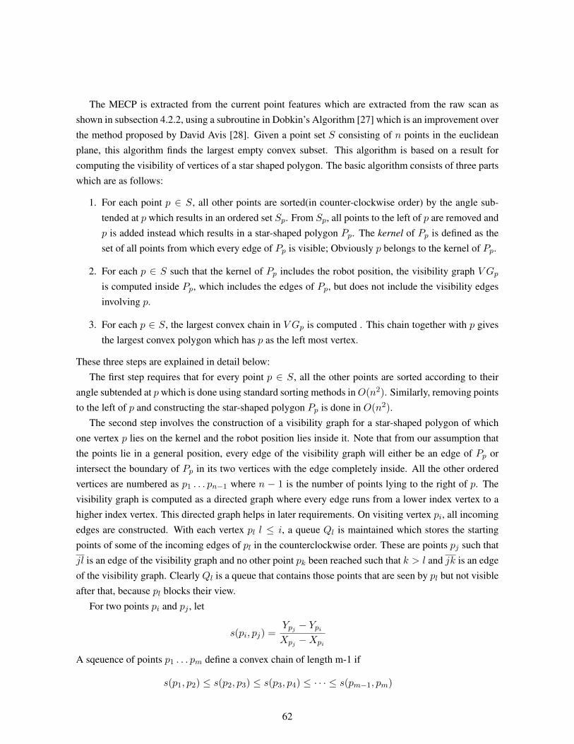
The MECP is extracted from the current point features which are extracted from the raw scan asshown in subsection 4.2.2, using a subroutine in Dobkin’s Algorithm [27] which is an improvement overthe method proposed by David Avis [28]. Given a point set S consisting of n points in the euclideanplane, this algorithm finds the largest empty convex subset. This algorithm is based on a result forcomputing the visibility of vertices of a star shaped polygon. The basic algorithm consists of three partswhich are as follows:

1. For each point p ∈ S, all other points are sorted(in counter-clockwise order) by the angle sub-tended at p which results in an ordered set Sp. From Sp, all points to the left of p are removed andp is added instead which results in a star-shaped polygon Pp. The kernel of Pp is defined as theset of all points from which every edge of Pp is visible; Obviously p belongs to the kernel of Pp.

2. For each p ∈ S such that the kernel of Pp includes the robot position, the visibility graph V Gpis computed inside Pp, which includes the edges of Pp, but does not include the visibility edgesinvolving p.

3. For each p ∈ S, the largest convex chain in V Gp is computed . This chain together with p givesthe largest convex polygon which has p as the left most vertex.

These three steps are explained in detail below:The first step requires that for every point p ∈ S, all the other points are sorted according to their

angle subtended at pwhich is done using standard sorting methods inO(n2). Similarly, removing pointsto the left of p and constructing the star-shaped polygon Pp is done in O(n2).

The second step involves the construction of a visibility graph for a star-shaped polygon of whichone vertex p lies on the kernel and the robot position lies inside it. Note that from our assumption thatthe points lie in a general position, every edge of the visibility graph will either be an edge of Pp orintersect the boundary of Pp in its two vertices with the edge completely inside. All the other orderedvertices are numbered as p1 . . . pn−1 where n − 1 is the number of points lying to the right of p. Thevisibility graph is computed as a directed graph where every edge runs from a lower index vertex to ahigher index vertex. This directed graph helps in later requirements. On visiting vertex pi, all incomingedges are constructed. With each vertex pl l ≤ i, a queue Ql is maintained which stores the startingpoints of some of the incoming edges of pl in the counterclockwise order. These are points pj such thatjl is an edge of the visibility graph and no other point pk been reached such that k > l and jk is an edgeof the visibility graph. Clearly Ql is a queue that contains those points that are seen by pl but not visibleafter that, because pl blocks their view.

For two points pi and pj , let

s(pi, pj) =Ypj − YpiXpj −Xpi

A sqeuence of points p1 . . . pm define a convex chain of length m-1 if

s(p1, p2) ≤ s(p2, p3) ≤ s(p3, p4) ≤ · · · ≤ s(pm−1, pm)

62

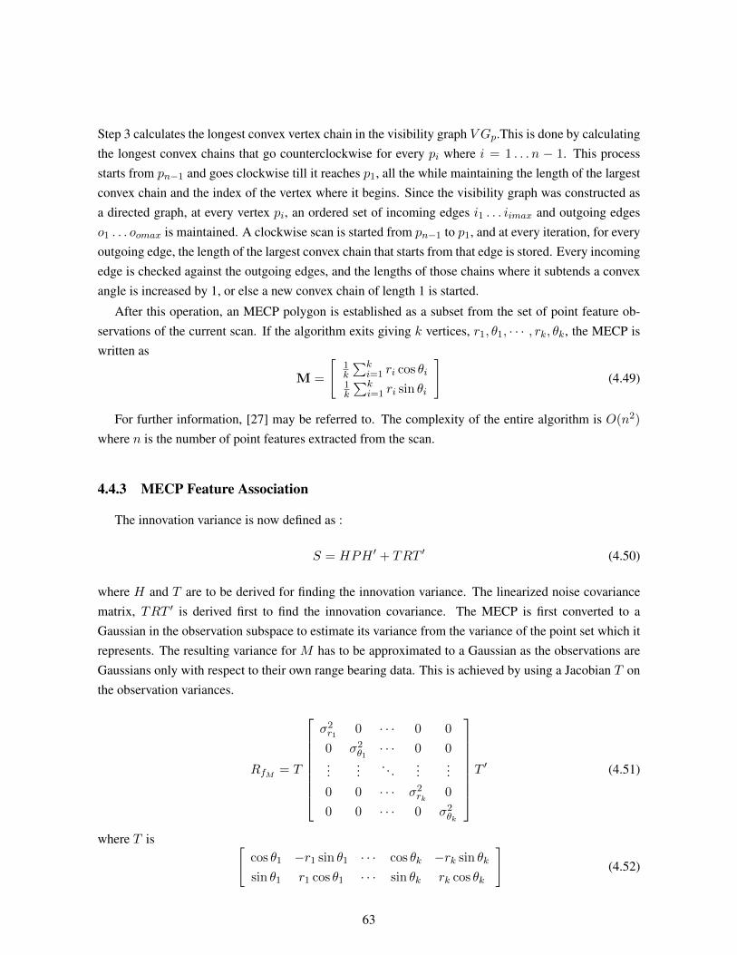
Step 3 calculates the longest convex vertex chain in the visibility graph V Gp.This is done by calculatingthe longest convex chains that go counterclockwise for every pi where i = 1 . . . n − 1. This processstarts from pn−1 and goes clockwise till it reaches p1, all the while maintaining the length of the largestconvex chain and the index of the vertex where it begins. Since the visibility graph was constructed asa directed graph, at every vertex pi, an ordered set of incoming edges i1 . . . iimax and outgoing edgeso1 . . . oomax is maintained. A clockwise scan is started from pn−1 to p1, and at every iteration, for everyoutgoing edge, the length of the largest convex chain that starts from that edge is stored. Every incomingedge is checked against the outgoing edges, and the lengths of those chains where it subtends a convexangle is increased by 1, or else a new convex chain of length 1 is started.

After this operation, an MECP polygon is established as a subset from the set of point feature ob-servations of the current scan. If the algorithm exits giving k vertices, r1, θ1, · · · , rk, θk, the MECP iswritten as

M =

[1k

∑ki=1 ri cos θi

1k

∑ki=1 ri sin θi

](4.49)

For further information, [27] may be referred to. The complexity of the entire algorithm is O(n2)

where n is the number of point features extracted from the scan.

4.4.3 MECP Feature Association

The innovation variance is now defined as :

S = HPH ′ + TRT ′ (4.50)

where H and T are to be derived for finding the innovation variance. The linearized noise covariancematrix, TRT ′ is derived first to find the innovation covariance. The MECP is first converted to aGaussian in the observation subspace to estimate its variance from the variance of the point set which itrepresents. The resulting variance for M has to be approximated to a Gaussian as the observations areGaussians only with respect to their own range bearing data. This is achieved by using a Jacobian T onthe observation variances.

RfM = T

σ2r1 0 · · · 0 0

0 σ2θ1· · · 0 0

......

. . ....

...0 0 · · · σ2

rk0

0 0 · · · 0 σ2θk

T ′ (4.51)

where T is [cos θ1 −r1 sin θ1 · · · cos θk −rk sin θk

sin θ1 r1 cos θ1 · · · sin θk rk cos θk

](4.52)

63

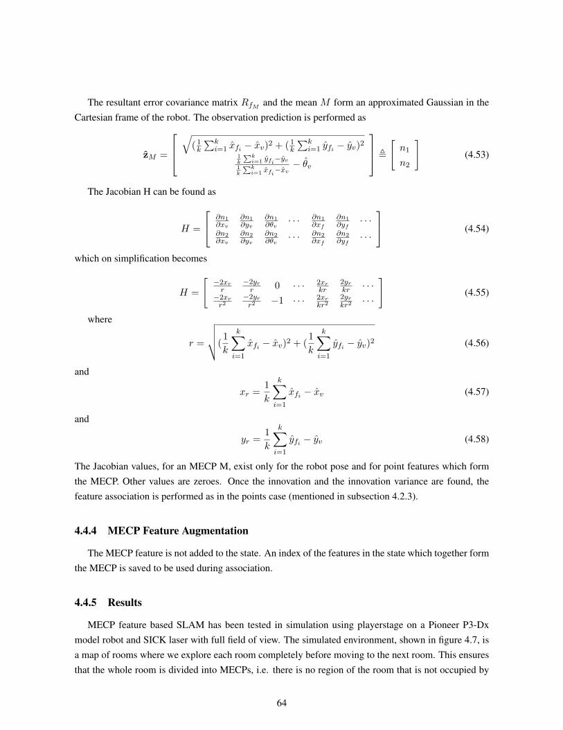
The resultant error covariance matrix RfM and the mean M form an approximated Gaussian in theCartesian frame of the robot. The observation prediction is performed as

zM =

√

( 1k

∑ki=1 xfi − xv)2 + ( 1

k

∑ki=1 yfi − yv)2

1k

∑ki=1 yfi−yv

1k

∑ki=1 xfi−xv

− θv

,

[n1

n2

](4.53)

The Jacobian H can be found as

H =

∂n1∂xv

∂n1∂yv

∂n1∂θv

· · · ∂n1∂xf

∂n1∂yf

· · ·∂n2∂xv

∂n2∂yv

∂n2∂θv

· · · ∂n2∂xf

∂n2∂yf

· · ·

(4.54)

which on simplification becomes

H =

[−2xrr

−2yrr 0 · · · 2xr

kr2yrkr · · ·

−2xrr2

−2yrr2

−1 · · · 2xrkr2

2yrkr2

· · ·

](4.55)

where

r =

√√√√(1

k

k∑i=1

xfi − xv)2 + (1

k

k∑i=1

yfi − yv)2 (4.56)

and

xr =1

k

k∑i=1

xfi − xv (4.57)

and

yr =1

k

k∑i=1

yfi − yv (4.58)

The Jacobian values, for an MECP M, exist only for the robot pose and for point features which formthe MECP. Other values are zeroes. Once the innovation and the innovation variance are found, thefeature association is performed as in the points case (mentioned in subsection 4.2.3).

4.4.4 MECP Feature Augmentation

The MECP feature is not added to the state. An index of the features in the state which together formthe MECP is saved to be used during association.

4.4.5 Results

MECP feature based SLAM has been tested in simulation using playerstage on a Pioneer P3-Dxmodel robot and SICK laser with full field of view. The simulated environment, shown in figure 4.7, isa map of rooms where we explore each room completely before moving to the next room. This ensuresthat the whole room is divided into MECPs, i.e. there is no region of the room that is not occupied by

64

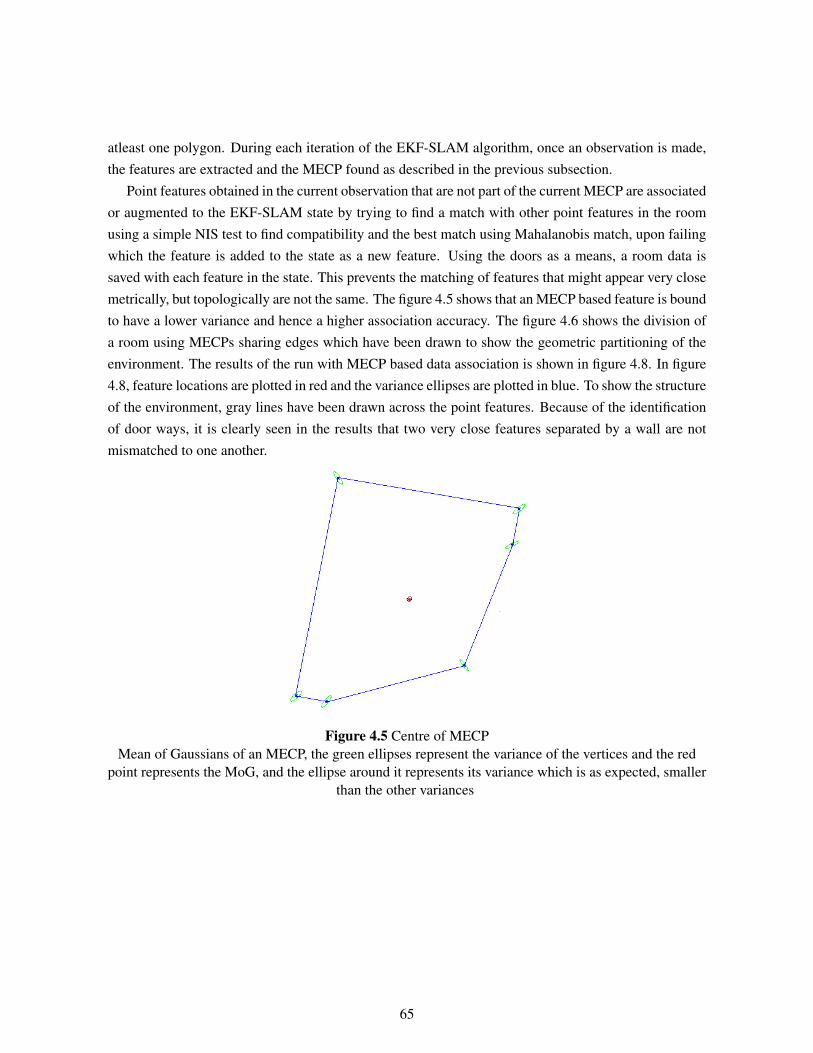
atleast one polygon. During each iteration of the EKF-SLAM algorithm, once an observation is made,the features are extracted and the MECP found as described in the previous subsection.

Point features obtained in the current observation that are not part of the current MECP are associatedor augmented to the EKF-SLAM state by trying to find a match with other point features in the roomusing a simple NIS test to find compatibility and the best match using Mahalanobis match, upon failingwhich the feature is added to the state as a new feature. Using the doors as a means, a room data issaved with each feature in the state. This prevents the matching of features that might appear very closemetrically, but topologically are not the same. The figure 4.5 shows that an MECP based feature is boundto have a lower variance and hence a higher association accuracy. The figure 4.6 shows the division ofa room using MECPs sharing edges which have been drawn to show the geometric partitioning of theenvironment. The results of the run with MECP based data association is shown in figure 4.8. In figure4.8, feature locations are plotted in red and the variance ellipses are plotted in blue. To show the structureof the environment, gray lines have been drawn across the point features. Because of the identificationof door ways, it is clearly seen in the results that two very close features separated by a wall are notmismatched to one another.

Figure 4.5 Centre of MECPMean of Gaussians of an MECP, the green ellipses represent the variance of the vertices and the red

point represents the MoG, and the ellipse around it represents its variance which is as expected, smallerthan the other variances

65

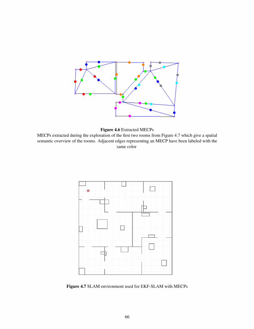
Figure 4.6 Extracted MECPsMECPs extracted during the exploration of the first two rooms from Figure 4.7 which give a spatialsemantic overview of the rooms. Adjacent edges representing an MECP have been labeled with the

same color

Figure 4.7 SLAM environment used for EKF-SLAM with MECPs

66

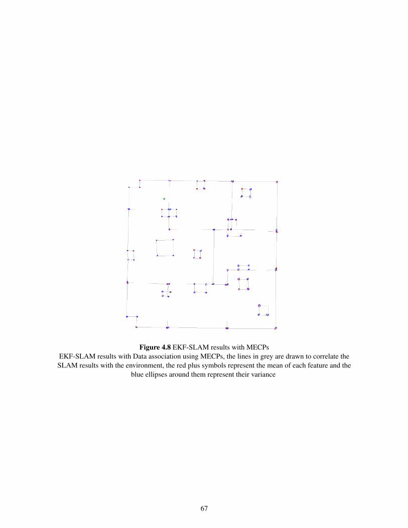
Figure 4.8 EKF-SLAM results with MECPsEKF-SLAM results with Data association using MECPs, the lines in grey are drawn to correlate theSLAM results with the environment, the red plus symbols represent the mean of each feature and the

blue ellipses around them represent their variance

67

4.5 Summary

This chapter discussed the use of different kinds of features for a laser based EKF-SLAM implemen-tation to increase the efficiency of the map building process.

The chapter begins with the details of a point feature based SLAM. The shortcomings of point basedSLAM is discussed next, followed by the details of a line feature based SLAM and its advantages over apoint feature based SLAM due to its greater visibility which keeps the heading error in check. The lastsection deals with MECP based features which tighten the bound for association of points by choosinga representative point for association and help in loop closing.

68

Chapter 5

Results

The results from the various experiments in this work have been displayed in this chapter. Thischapter attempts to maintain a chronological order of results as have been achieved so as to providean understanding of the evolution of the work. The experiments conducted begin with simulation andthen move to environments where artificial features are used for mapping. This is followed by resultsfrom mapping in natural indoor environments with no modifications where we report a satisfactoryperformance in different environments.

5.1 Experiments in modelled environments

This section is a set of results generated on artificial maps, maps which have been either hand-madeor altered for testing EKF-SLAM.

5.1.1 Simulated Environment

The below figure with four sub-figures is the output of a simulation EKF-SLAM run in an artificialmap as shown in figure 5.1(a). The second sub-figure 5.1(b) has been taken after some iterations ofthe algorithm. The robot is visible as a circle with a green variance ellipse and the point features asred cross symbols with blue variance ellipses. The third sub-figure 5.2(a) has been taken just beforethe robot observes a feature with very low uncertainty. A low uncertainty feature is a feature seen inone of the earlier iterations of the algorithm, whose observation reduces the variance of the completestate vector. This property, called loop closing, is evident in the next sub-figure 5.2(b) as the map errorsreduce due to the covariance between the features through the robot.

69

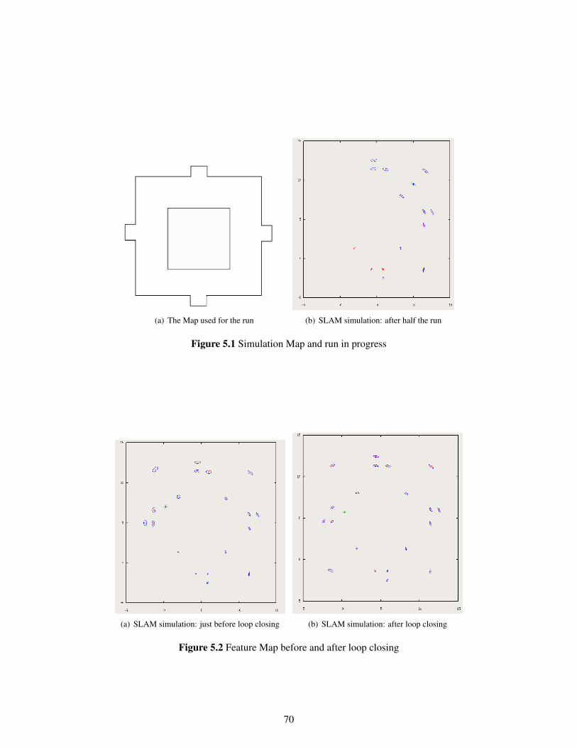
(a) The Map used for the run (b) SLAM simulation: after half the run

Figure 5.1 Simulation Map and run in progress

(a) SLAM simulation: just before loop closing (b) SLAM simulation: after loop closing

Figure 5.2 Feature Map before and after loop closing

70

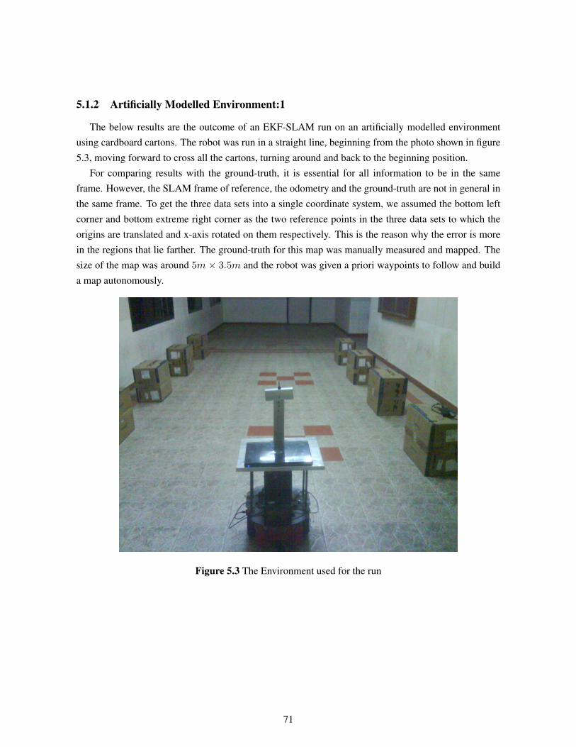
5.1.2 Artificially Modelled Environment:1

The below results are the outcome of an EKF-SLAM run on an artificially modelled environmentusing cardboard cartons. The robot was run in a straight line, beginning from the photo shown in figure5.3, moving forward to cross all the cartons, turning around and back to the beginning position.

For comparing results with the ground-truth, it is essential for all information to be in the sameframe. However, the SLAM frame of reference, the odometry and the ground-truth are not in general inthe same frame. To get the three data sets into a single coordinate system, we assumed the bottom leftcorner and bottom extreme right corner as the two reference points in the three data sets to which theorigins are translated and x-axis rotated on them respectively. This is the reason why the error is morein the regions that lie farther. The ground-truth for this map was manually measured and mapped. Thesize of the map was around 5m× 3.5m and the robot was given a priori waypoints to follow and builda map autonomously.

Figure 5.3 The Environment used for the run

71

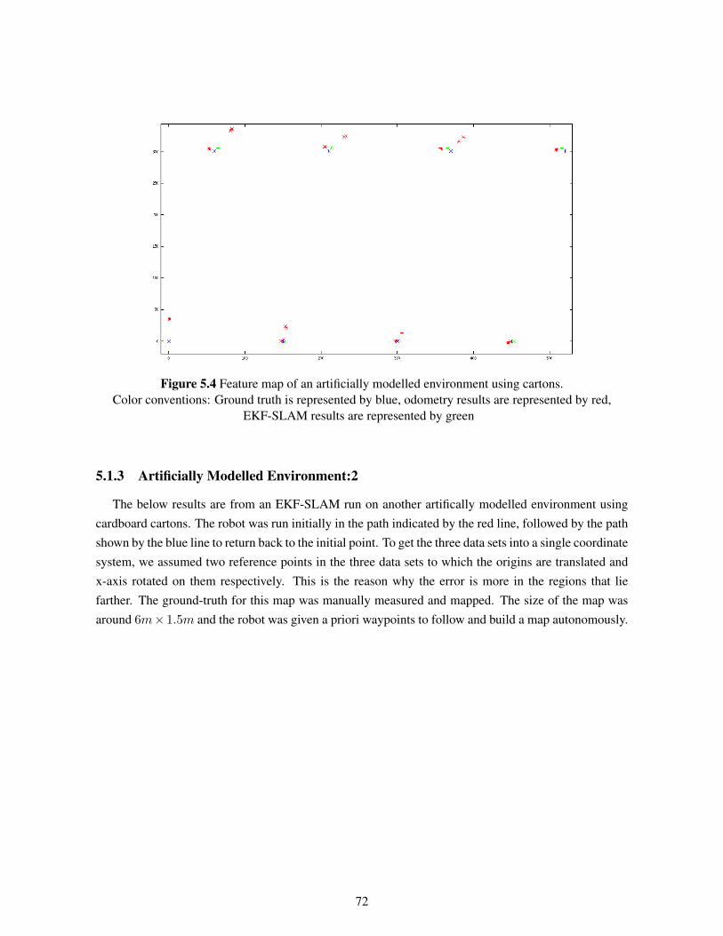
Figure 5.4 Feature map of an artificially modelled environment using cartons.Color conventions: Ground truth is represented by blue, odometry results are represented by red,

EKF-SLAM results are represented by green

5.1.3 Artificially Modelled Environment:2

The below results are from an EKF-SLAM run on another artifically modelled environment usingcardboard cartons. The robot was run initially in the path indicated by the red line, followed by the pathshown by the blue line to return back to the initial point. To get the three data sets into a single coordinatesystem, we assumed two reference points in the three data sets to which the origins are translated andx-axis rotated on them respectively. This is the reason why the error is more in the regions that liefarther. The ground-truth for this map was manually measured and mapped. The size of the map wasaround 6m× 1.5m and the robot was given a priori waypoints to follow and build a map autonomously.

72

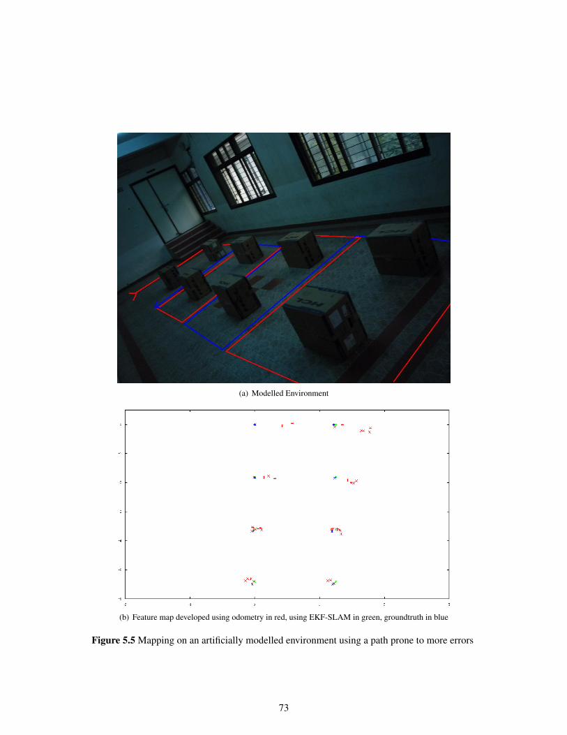
(a) Modelled Environment

(b) Feature map developed using odometry in red, using EKF-SLAM in green, groundtruth in blue

Figure 5.5 Mapping on an artificially modelled environment using a path prone to more errors

73

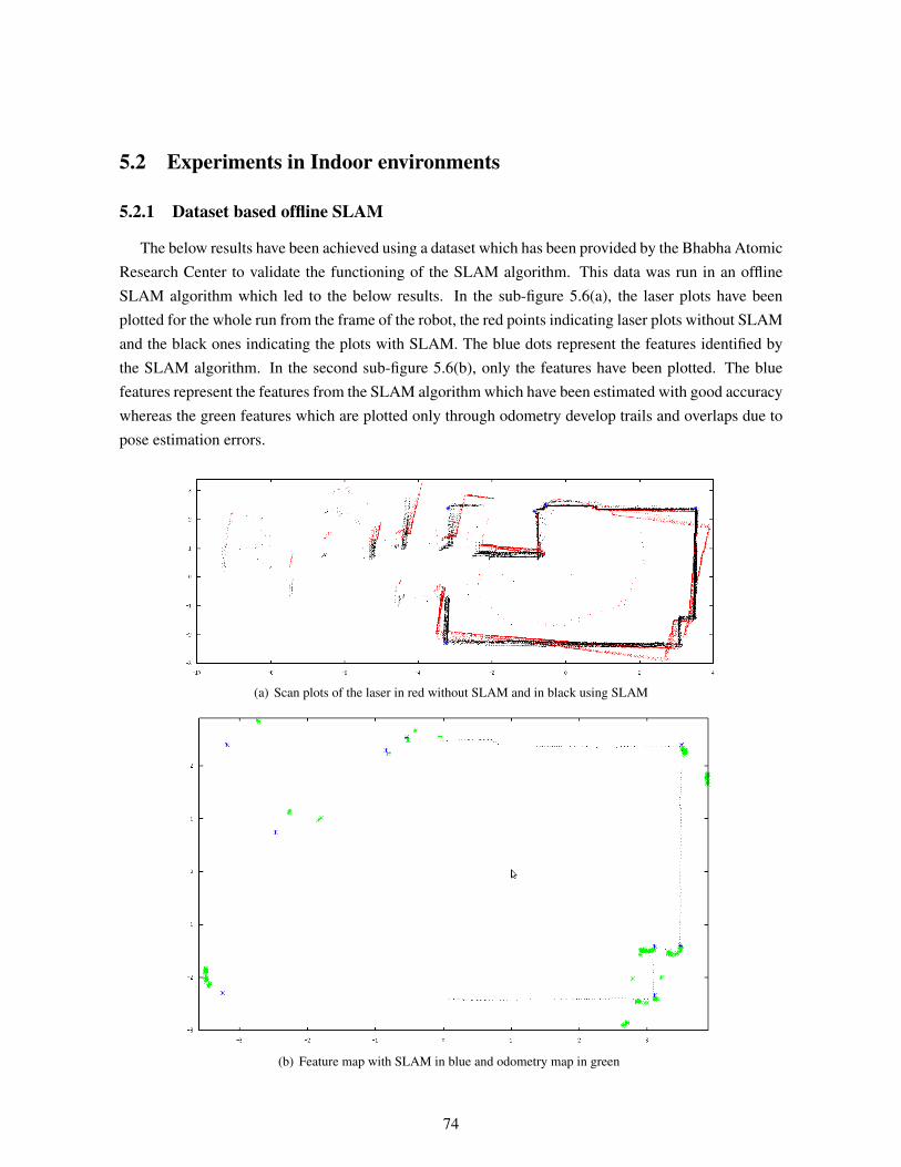
5.2 Experiments in Indoor environments

5.2.1 Dataset based offline SLAM

The below results have been achieved using a dataset which has been provided by the Bhabha AtomicResearch Center to validate the functioning of the SLAM algorithm. This data was run in an offlineSLAM algorithm which led to the below results. In the sub-figure 5.6(a), the laser plots have beenplotted for the whole run from the frame of the robot, the red points indicating laser plots without SLAMand the black ones indicating the plots with SLAM. The blue dots represent the features identified bythe SLAM algorithm. In the second sub-figure 5.6(b), only the features have been plotted. The bluefeatures represent the features from the SLAM algorithm which have been estimated with good accuracywhereas the green features which are plotted only through odometry develop trails and overlaps due topose estimation errors.

(a) Scan plots of the laser in red without SLAM and in black using SLAM

(b) Feature map with SLAM in blue and odometry map in green

74

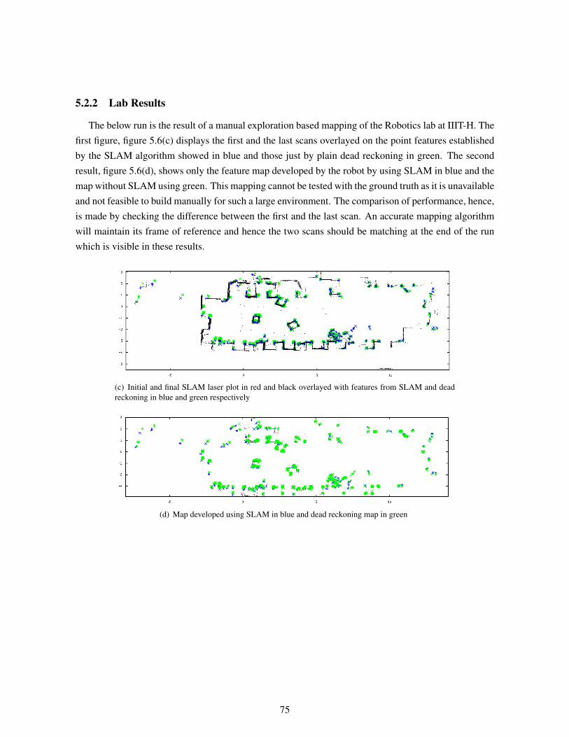
5.2.2 Lab Results

The below run is the result of a manual exploration based mapping of the Robotics lab at IIIT-H. Thefirst figure, figure 5.6(c) displays the first and the last scans overlayed on the point features establishedby the SLAM algorithm showed in blue and those just by plain dead reckoning in green. The secondresult, figure 5.6(d), shows only the feature map developed by the robot by using SLAM in blue and themap without SLAM using green. This mapping cannot be tested with the ground truth as it is unavailableand not feasible to build manually for such a large environment. The comparison of performance, hence,is made by checking the difference between the first and the last scan. An accurate mapping algorithmwill maintain its frame of reference and hence the two scans should be matching at the end of the runwhich is visible in these results.

(c) Initial and final SLAM laser plot in red and black overlayed with features from SLAM and deadreckoning in blue and green respectively

(d) Map developed using SLAM in blue and dead reckoning map in green

75

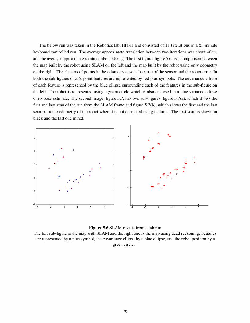
The below run was taken in the Robotics lab, IIIT-H and consisted of 113 iterations in a 25 minutekeyboard controlled run. The average approximate translation between two iterations was about 40cm

and the average approximate rotation, about 45 deg. The first figure, figure 5.6, is a comparison betweenthe map built by the robot using SLAM on the left and the map built by the robot using only odometryon the right. The clusters of points in the odometry case is because of the sensor and the robot error. Inboth the sub-figures of 5.6, point features are represented by red plus symbols. The covariance ellipseof each feature is represented by the blue ellipse surrounding each of the features in the sub-figure onthe left. The robot is represented using a green circle which is also enclosed in a blue variance ellipseof its pose estimate. The second image, figure 5.7, has two sub-figures, figure 5.7(a), which shows thefirst and last scan of the run from the SLAM frame and figure 5.7(b), which shows the first and the lastscan from the odometry of the robot when it is not corrected using features. The first scan is shown inblack and the last one in red.

Figure 5.6 SLAM results from a lab runThe left sub-figure is the map with SLAM and the right one is the map using dead reckoning. Featuresare represented by a plus symbol, the covariance ellipse by a blue ellipse, and the robot position by a

green circle.

76

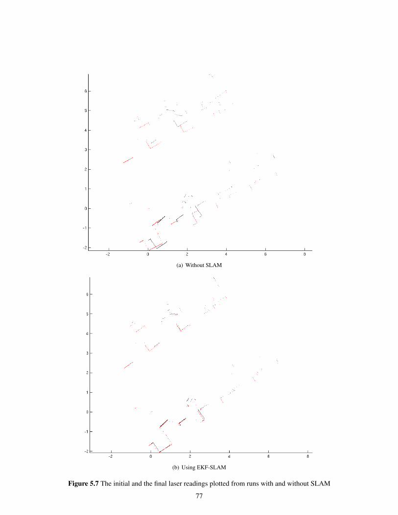
(a) Without SLAM

(b) Using EKF-SLAM

Figure 5.7 The initial and the final laser readings plotted from runs with and without SLAM

77

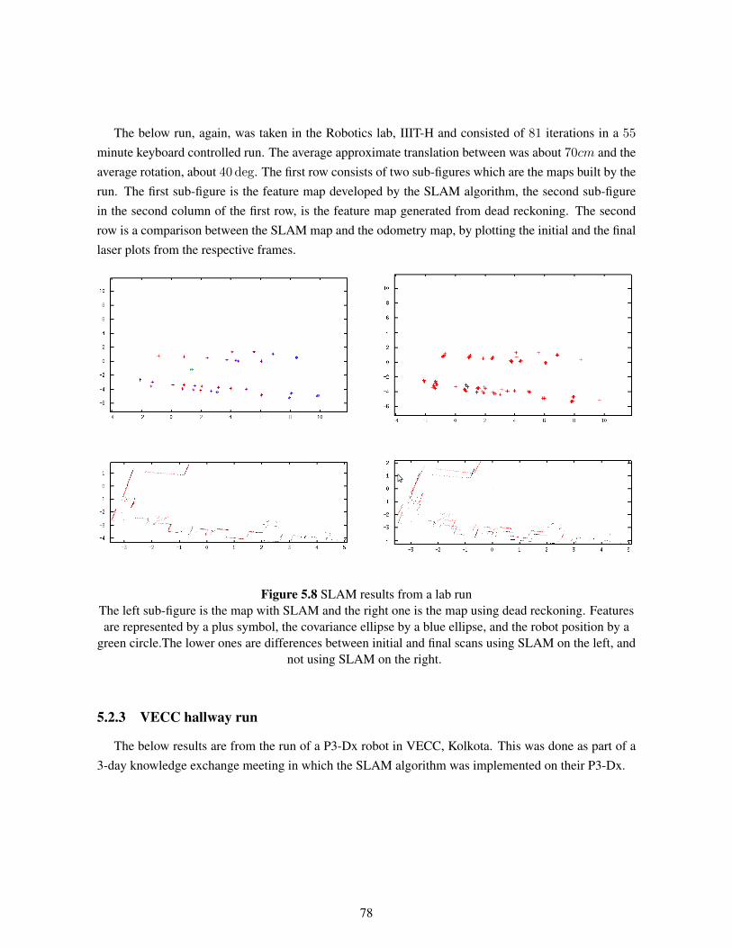
The below run, again, was taken in the Robotics lab, IIIT-H and consisted of 81 iterations in a 55

minute keyboard controlled run. The average approximate translation between was about 70cm and theaverage rotation, about 40 deg. The first row consists of two sub-figures which are the maps built by therun. The first sub-figure is the feature map developed by the SLAM algorithm, the second sub-figurein the second column of the first row, is the feature map generated from dead reckoning. The secondrow is a comparison between the SLAM map and the odometry map, by plotting the initial and the finallaser plots from the respective frames.

Figure 5.8 SLAM results from a lab runThe left sub-figure is the map with SLAM and the right one is the map using dead reckoning. Featuresare represented by a plus symbol, the covariance ellipse by a blue ellipse, and the robot position by a

green circle.The lower ones are differences between initial and final scans using SLAM on the left, andnot using SLAM on the right.

5.2.3 VECC hallway run

The below results are from the run of a P3-Dx robot in VECC, Kolkota. This was done as part of a3-day knowledge exchange meeting in which the SLAM algorithm was implemented on their P3-Dx.

78

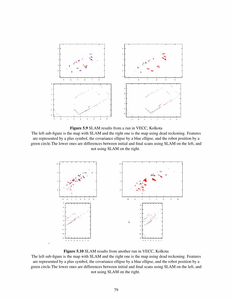
Figure 5.9 SLAM results from a run in VECC, KolkotaThe left sub-figure is the map with SLAM and the right one is the map using dead reckoning. Featuresare represented by a plus symbol, the covariance ellipse by a blue ellipse, and the robot position by a

green circle.The lower ones are differences between initial and final scans using SLAM on the left, andnot using SLAM on the right.

Figure 5.10 SLAM results from another run in VECC, KolkotaThe left sub-figure is the map with SLAM and the right one is the map using dead reckoning. Featuresare represented by a plus symbol, the covariance ellipse by a blue ellipse, and the robot position by a

green circle.The lower ones are differences between initial and final scans using SLAM on the left, andnot using SLAM on the right.

79

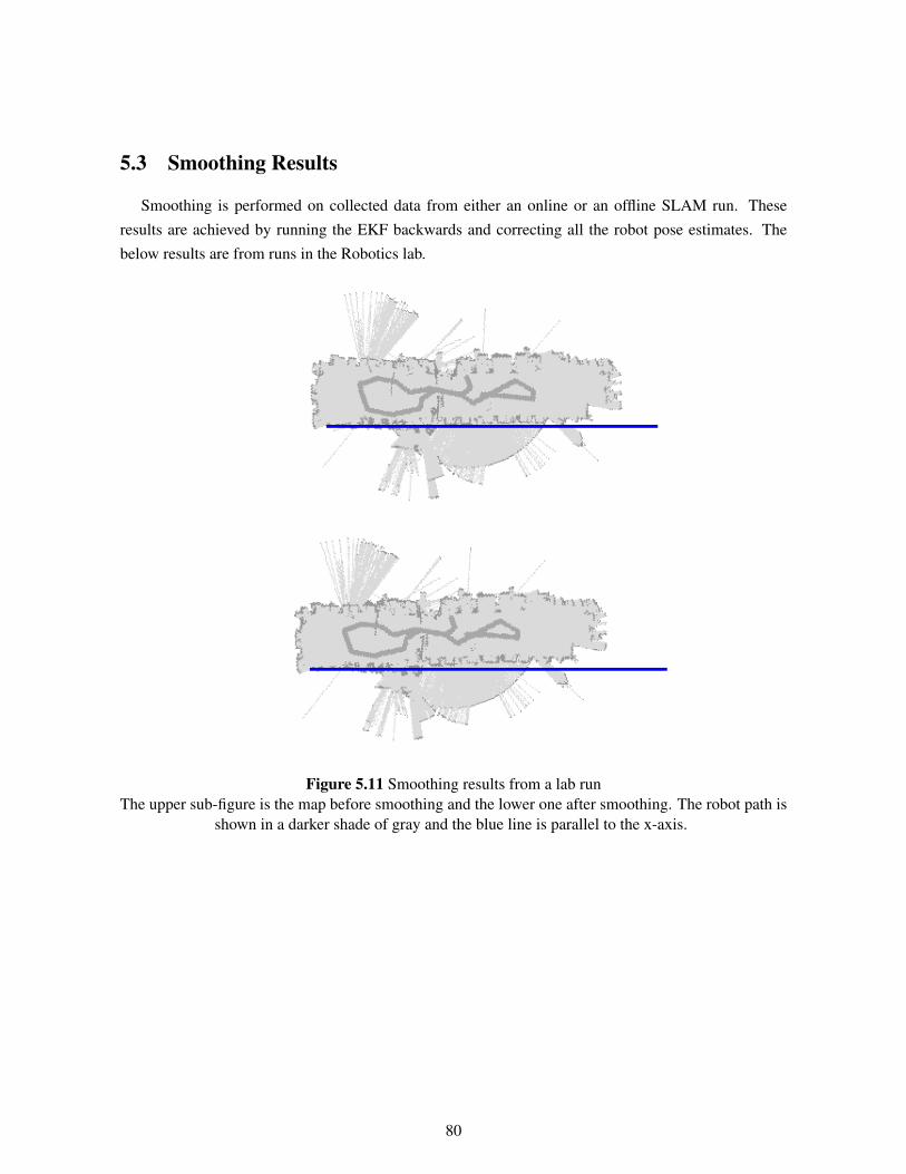
5.3 Smoothing Results

Smoothing is performed on collected data from either an online or an offline SLAM run. Theseresults are achieved by running the EKF backwards and correcting all the robot pose estimates. Thebelow results are from runs in the Robotics lab.

Figure 5.11 Smoothing results from a lab runThe upper sub-figure is the map before smoothing and the lower one after smoothing. The robot path is

shown in a darker shade of gray and the blue line is parallel to the x-axis.

80

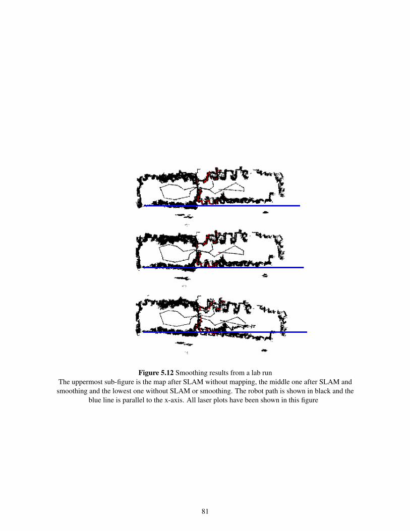
Figure 5.12 Smoothing results from a lab runThe uppermost sub-figure is the map after SLAM without mapping, the middle one after SLAM and

smoothing and the lowest one without SLAM or smoothing. The robot path is shown in black and theblue line is parallel to the x-axis. All laser plots have been shown in this figure

81

Chapter 6

Conclusions

In this thesis, we have discussed the problem of autonomous mapping and have developed a realmapping system. We started the thesis with an introduction to the Simultaneous Localization AndMapping problem and its importance in the field of mobile robotics. We then introduced a probabilisticmethod to solve the SLAM problem, called the Extended Kalman Filter based SLAM. This was followedup by the system specific customizations that were required to develop a real SLAM implementation.This included building the algorithm with the appropriate vehicle and sensor models, followed by theessential sensor to robot calibration algorithm to reduce errors due to different reference frames andfinally smoothing to develop maps where path planning can be performed. The next part of this thesisdelved into different kinds of features to be used as observations in the SLAM algorithm for the purposeof map building. Point feature based SLAM, which has been implemented and tested as a real systemhas been discussed in detail. This is followed by its shortcomings and using line based features andMECP based features for better feature association and eventually better map building.

This chapter is a concise interpretation of the knowledge attained from the work undergone towardsthe development of this thesis.

6.1 Calibration

The immediate problem with implementing a SLAM algorithm on a custom hardware platform hasbeen identified as that of differences in the reference frames of the laser and the robot. Our first systemimplementation did not consider these issues and assumed variances as described in the hardware man-ual while ignoring system specific details. The algorithm thus implemented, clearly showed erroneousresults even in simple and short maps. Upon close inspection, the different frames of reference wereobserved and identified as the problem. This led to the development of the calibration algorithm, valuesfrom which when used into the SLAM algorithm proved highly rewarding in the form of accurate maps.The first conclusion from this work is the essential requirement of a well-calibrated system with knownerror variances, which is a pre-requisite for building good maps.

82

6.2 Smoothing

Development of a feature based map is very essential for the purpose of localization for a mobilerobot in a given environment. However, the inability to use the map to be able to plan its path from onepoint to another was another problem addressed in this work. The lack of the availability of the trajectoryof the robot was identified as the principal reason for the absence of a more informative map. The fullSLAM algorithm, which also provides the trajectory of the robot was found to be of high computationalcomplexity.

This led to the usage of an Extended Kalman smoother on robot pose estimates from a SLAMrun. Smoothing is performed by running the EKF backwards from the last iteration of the SLAMalgorithm to the first iteration. Each iteration uses the last corrected robot pose data to correct robotposes, earlier in time, which might have gained high levels of inaccuracy during the course of the run,due to unavailability of features with low error. Smoothing provides a more accurate set of robot poseswhich can be used to develop a complete metric map, a map with all the information given by the rangescanner in the form of a map.

6.3 Features

During the course of experiments on SLAM, the importance of feature association was evident.Errors in the robot would eventually lead to the breakdown of the association process, leading to thefailure of the SLAM algorithm. An efficient deployment of SLAM thus required keeping the robotpose error in check by observing features regularly. It was observed that point features were not visiblein numerous environments for long times causing the robot to gain error. To keep the robot error incheck, the robot heading error was identified as the main culprit. The robot heading error was then keptin check by the use of line based features with higher visibility than point features leading to bettermaps. This was followed by an attempt to utilize the geometric relation between point features forensuring accurate associations. The issue of feature matching based on nearness would often lead to thematching of features close in space but not topologically, thus making the map erroneous. An MECPbased matching coupled with a simple door identification helped in stopping this erroneous association.

6.4 Non-linearity Issues

The EKF-SLAM can be thought of as a KF-SLAM with some wrapping to handle non-linearity.Non-linearity is implicit in the system which makes it essential to deal with it. The EKF system handlesnon-linearity by the use of a first order Taylor series approximation of the non-linear functions. This ap-proximation has been documented to be overconfident and in some cases leading to erroneous estimatesand eventually to inefficient maps. Although, the EKF-SLAM system has performed in our differentfeature experiments which use approximations, it was at times observed that high non-linearity errors

83

would lead to a breakdown of the algorithm. This issue comes implicitly with the EKF-SLAM system,although reduction in non-linearity errors has been done using ??.

6.5 Scope

This work uses an EKF-SLAM based technique and works on improvizing its performance throughvarious combinations of features. The scope for this work is present primarily in the sense of solv-ing problems coupled with the one being addressed. Specifically, there is scope towards work in twodirections, implementation and theory.

6.5.1 Implementation based scope

We have developed a working SLAM system during the course of this work. This system is capableof developing feature maps when guided through the environment or given a priori waypoints. However,we believe that the below contributions to the implementation will be invaluable:

• Path planning using complete metric maps

• SLAM with exploration

6.5.1.1 Path planning using complete metric maps

The smoothing based maps developed by the offline run in reverse of a completed SLAM test can beused by the robot for the purpose of path planning. However, this provision has not been implementedin the system. A robot performing a SLAM algorithm, followed by smoothing of its trajectory to get acomplete metric map and using it to navigate itself while avoiding obstacles would be a complete systemin itself that can be one of a kind with complete functionalities: localization, mapping and navigation,thus providing an autonomous system with great capabilities.

6.5.1.2 SLAM with Exploration

The SLAM system deployed in this work is not accompanied with an exploration algorithm withobstacle avoidance to autonomously traverse an unknown environment completely and develop a mapof it. This added enhancement would ensure a completely autonomous mapping system.

6.5.2 Theory based scope

We have worked on developing complete metric maps and using novel feature parametrizations toimprove SLAM in static environments. we believe that there is scope for further work in:

• SLAM with Exploration

84

• Better features and feature association

• SLAM in a dynamic environment

• SLAM using sensor fusion

6.5.2.1 SLAM with Exploration

An exploration algorithm that would explore the environment in an intelligent manner by locating thebest frontier for it to reduce its pose variance and thus keep the error low, would be a great contributionto develop better maps using SLAM.

6.5.2.2 Better Features and Feature association

We have showcased our work on the parametrization of a few features which has aided in improvingthe efficiency of SLAM. However, we believe that there is immense scope towards work on developingfeatures which encompass geometric information of the environment in different ways which can helpin better feature association

6.5.2.3 SLAM in a dynamic environment

The maps developed in this work assume the environment to be static and hence the algorithm isnot built to handle dynamic environments. However, given recent work on localization in dynamicenvironments, there is tremendous scope for developing a SLAM system which can function in dynamicenvironments tracking both static and non-static features.

6.5.2.4 SLAM using sensor fusion

The use of a vision sensor to label features identified by the laser also using a color constraint canmake the feature association algorithm more robust and improve in mapping.

6.6 Summary

We conclude this thesis in the sincere hope that it will serve as an informative reference for interestedindividuals in the field of mobile robotics. We hope that the documented code and the deployed systemwill serve as good starting points to grasp the concepts of mapping. We believe that this thesis providesa comprehensive and simplistic view of EKF-SLAM while also discussing about system specific de-tails which are necessary for the implementation of any mapping algorithm. We end this thesis in theanticipation that it might serve as a knowledge resource for further research and contribute towards thegrowth of the robotics community.

85

Related Publications

• Data Association using Empty Convex Polygonal Regions in EKF-SLAM, Gururaj Kosuru,Satish Pedduri and K Madhava KrishnaIEEE International Conference on Robotics and Biomimetics, 2010

• On Measurement Models for Line Segments and Point Based SLAM, Satish Pedduri, GururajKosuru, K Madhava Krishna and Amit K PandeyIEEE International Conference on Advanced Robotics, 2009

86

Bibliography

[1] S.B. Williams. Efficient solutions to autonomous mapping and navigation problems. PhD thesis,Australian Centre for Field Robotics, 2001.

[2] D. Fox, W. Burgard, and S. Thrun. Markov localization for mobile robots in dynamic environ-ments. Journal of Artificial Intelligence Research, 11(3):391–427, 1999.

[3] H.P. Moravec. Sensor fusion in certainty grids for mobile robots. AI magazine, 9(2):61, 1988.

[4] J.J. Leonard, H.F. Durrant-Whyte, and I.J. Cox. Dynamic map building for an autonomous mobilerobot. The International Journal of Robotics Research, 11(4):286, 1992.

[5] H. Durrant-Whyte and T. Bailey. Simultaneous localisation and mapping (SLAM): Part I theessential algorithms. Robotics and Automation Magazine, 13(2):99–110, 2006.

[6] J.J. Leonard and H.F. Durrant-Whyte. Simultaneous map building and localization for an au-tonomous mobile robot. In Intelligent Robots and Systems’ 91.’Intelligence for Mechanical Sys-tems, Proceedings IROS’91. IEEE/RSJ International Workshop on, pages 1442–1447. IEEE, 2002.

[7] R. Smith, M. Self, and P. Cheeseman. A stochastic map for uncertain spatial relationships. InProceedings of the 4th international symposium on Robotics Research, page 474. MIT Press, 1988.

[8] R. Smith, M. Self, and P. Cheeseman. Estimating uncertain spatial relationships in robotics. Au-tonomous robot vehicles, 1:167–193, 1990.

[9] R. Chatila and J. Laumond. Position referencing and consistent world modeling for mobile robots.In Robotics and Automation. Proceedings. 1985 IEEE International Conference on, volume 2,pages 138–145. IEEE, 2002.

[10] H. Durrant-Whyte, D. Rye, and E. Nebot. Localisation of automatic guided vehicles,. In RoboticsResearch: The 7th International Symposium(ISRR), 1995.

[11] M. Csorba. Simultaneous Localisation And Map Building. PhD thesis, University of Oxford, 1997.

[12] J.A. Castellanos, JM Martnez, J. Neira, and J.D. Tardos. Experiments in multisensor mobile robotlocalization and map building. Proc. 3rd IFAC Sym. Intell. Auton. Vehicles, pages 173–178, 1998.

87

[13] JA Castellanos, JD Tardos, and G. Schmidt. Building a global map of the environment of a mobilerobot: The importance of correlations. In Robotics and Automation, 1997. Proceedings., 1997IEEE International Conference on, volume 2, pages 1053–1059. IEEE, 2002.

[14] J.J. Leonard and H.J.S. Feder. A computationally efficient method for large-scale concurrent map-ping and localization. In Robotics Research, The ninth International Symposium(ISRR’99), vol-ume 9, pages 169–178. Citeseer, 2000.

[15] S. Thrun, W. Burgard, and D. Fox. A probabilistic approach to concurrent mapping and localiza-tion for mobile robots. Autonomous Robots, 5(3):253–271, 1998.

[16] S.J. Julier and J.K. Uhlmann. A new extension of the Kalman filter to nonlinear systems. In Int.Symp. Aerospace/Defense Sensing, Simul. and Controls, volume 3, page 26, 1997.

[17] J. Leonard and P. Newman. Consistent, convergent, and constant-time SLAM. In InternationalJoint Conference on Artificial Intelligence, volume 18, pages 1143–1150, 2003.

[18] M. Kaess, A. Ranganathan, and F. Dellaert. iSAM: Incremental smoothing and mapping. Robotics,IEEE Transactions on, 24(6):1365–1378, 2008.

[19] R.E. Kalman et al. A new approach to linear filtering and prediction problems. Journal of basicEngineering, 82(1):35–45, 1960.

[20] P. Newman. On the structure and solution of the simultaneous localisation and map buildingproblem. PhD thesis, Ph. D. thesis, Australian Centre for Field Robotics, University of Sydney,Australia, 2000.

[21] A. Garulli, A. Giannitrapani, A. Rossi, and A. Vicino. Mobile robot SLAM for line-based envi-ronment representation. In Decision and Control, 2005 and 2005 European Control Conference.CDC-ECC’05. 44th IEEE Conference on, pages 2041–2046. IEEE, 2005.

[22] A. Gee and W. Mayol-Cuevas. Real-time model-based slam using line segments. Advances inVisual Computing, pages 354–363, 2006.

[23] T. Lemaire and S. Lacroix. Monocular-vision based SLAM using line segments. In Robotics andAutomation, 2007 IEEE International Conference on, pages 2791–2796. IEEE, 2007.

[24] V. Nguyen, A. Martinelli, N. Tomatis, and R. Siegwart. A comparison of line extraction algo-rithms using 2D laser rangefinder for indoor mobile robotics. In Intelligent Robots and Systems,2005.(IROS 2005). 2005 IEEE/RSJ International Conference on, pages 1929–1934. IEEE, 2005.

[25] Y.H. Choi, T.K. Lee, and S.Y. Oh. A line feature based SLAM with low grade range sensors usinggeometric constraints and active exploration for mobile robot. Autonomous Robots, 24(1):13–27,2008.

88

[26] C.P. Connette, O. Meister, M. Hagele, and G.F. Trommer. Decomposition of line segments intocorner and statistical grown line features in an EKF-SLAM framework. In Intelligent Robots andSystems, 2007. IROS 2007. IEEE/RSJ International Conference on, pages 3884–3891. IEEE, 2007.

[27] D.P. Dobkin, H. Edelsbrunner, and M.H. Overmars. Searching for empty convex polygons. Algo-rithmica, 5(1):561–571, 1990.

[28] D. Avis and D. Rappaport. Computing the largest empty convex subset of a set of points. InProceedings of the first annual symposium on Computational geometry, pages 161–167. ACM,1985.

[29] T. Bailey. Mobile robot localisation and mapping in extensive outdoor environments. PhD thesis,Australian Centre for Field Robotics, 2002.

[30] S. Thrun, W. Burgard, and D. Fox. Probabilistic robotics. 2005.

[31] T. Bailey and H. Durrant-Whyte. Simultaneous localization and mapping (SLAM): Part II.Robotics & Automation Magazine, IEEE, 13(3):108–117, 2006.

[32] P.S. Maybeck. Stochastic models, estimation, and control. Academic press, 1979.

[33] J. Sola. Towards visual localization, mapping and moving objects tracking by a mobile robot: ageometric and probabilistic approach. PhD thesis, PhD thesis, LAAS, Toulouse, 2007.

[34] Y. Bar-Shalom, X.R. Li, X.R. Li, and T. Kirubarajan. Estimation with applications to tracking andnavigation. Wiley-Interscience, 2001.

[35] J.J. Leonard and H.F. Durrant-Whyte. Mobile robot localization by tracking geometric beacons.Robotics and Automation, IEEE Transactions on, 7(3):376–382, 1991.

[36] D. Hahnel, S. Thrun, B. Wegbreit, and W. Burgard. Towards lazy data association in SLAM.Robotics Research, pages 421–431, 2005.

[37] R. Smith, M. Self, and P. Cheeseman. A stochastic map for uncertain spatial relationships. InProceedings of the 4th international symposium on Robotics Research, pages 467–474. MIT Press,1988.

[38] J. Neira and J.D. Tardos. Data association in stochastic mapping using the joint compatibility test.Robotics and Automation, IEEE Transactions on, 17(6):890–897, 2001.

[39] R. Vazquez-Martın, JC del Toro, A. Bandera, and F. Sandoval. Natural landmark extraction formobile robot navigation based on an adaptive curvature estimation. Robotics and AutonomousSystems, 56(3):247–264, 2008.

[40] C. Fernandez, V. Moreno, B. Curto, and J.A. Vicente. Clustering and line detection in laser rangemeasurements. Robotics and Autonomous Systems, 58(5):720–726, 2010.

89

[41] K.C.J. Dietmayer, J. Sparbert, and D. Streller. Model based object classification and object trackingin traffic scenes from range images. Proceedings of IV, pages 2–1, 2001.

[42] M. Bosse, P. Newman, J. Leonard, M. Soika, W. Feiten, and S. Teller. An atlas framework forscalable mapping. In Robotics and Automation, 2003. Proceedings. ICRA’03. IEEE InternationalConference on, volume 2, pages 1899–1906. IEEE, 2003.

[43] R. Martinez-Cantin and J.A. Castellanos. Bounding uncertainty in EKF-SLAM: the robocentriclocal approach. In Robotics and Automation, 2006. ICRA 2006. Proceedings 2006 IEEE Interna-tional Conference on, pages 430–435. IEEE, 2006.

[44] G.A. Borges and M.J. Aldon. Line extraction in 2D range images for mobile robotics. Journal ofIntelligent and Robotic Systems, 40(3):267–297, 2004.

[45] J. Nieto, T. Bailey, and E. Nebot. Scan-slam: Combining ekf-slam and scan correlation. In Fieldand Service Robotics, pages 167–178. Springer, 2006.

[46] G.P. Huang, A.I. Mourikis, and S.I. Roumeliotis. Analysis and improvement of the consistencyof extended Kalman filter based SLAM. In Robotics and Automation, 2008. ICRA 2008. IEEEInternational Conference on, pages 473–479. IEEE, 2008.

[47] S. Huang and G. Dissanayake. Convergence and consistency analysis for extended Kalman filterbased SLAM. Robotics, IEEE Transactions on, 23(5):1036–1049, 2007.

[48] G. Huang, A. Mourikis, and S. Roumeliotis. A first-estimates Jacobian EKF for improving SLAMconsistency. In Experimental Robotics, pages 373–382. Springer, 2009.

[49] J. Folkesson and H. Christensen. Graphical SLAM-a self-correcting map. In Robotics and Au-tomation, 2004. Proceedings. ICRA’04. 2004 IEEE International Conference on, volume 1, pages383–390. IEEE, 2004.

[50] J. Folkesson and H. Christensen. Outdoor exploration and slam using a compressed filter. In IEEEInternational Conference on Robotics and Automation, volume 1, pages 419–426. IEEE; 1999,2003.

[51] J. Neira and JD Tardos. Robust and feasible data association for simultaneous localization andmap building. In IEEE conference on Robotic and Automation, Workshop W, volume 4, 2000.

[52] D. Rodriguez-Losada, F. Matia, A. Jimenez, and R. Galan. Consistency improvement for SLAM-EKF for indoor environments. In Robotics and Automation, 2006. ICRA 2006. Proceedings 2006IEEE International Conference on, pages 418–423. IEEE, 2006.

[53] T. Bailey, J. Nieto, J. Guivant, M. Stevens, and E. Nebot. Consistency of the EKF-SLAM al-gorithm. In Intelligent Robots and Systems, 2006 IEEE/RSJ International Conference on, pages3562–3568. IEEE, 2006.

90

[54] M.W.M.G. Dissanayake, P. Newman, S. Clark, H.F. Durrant-Whyte, and M. Csorba. A solutionto the simultaneous localization and map building (SLAM) problem. Robotics and Automation,IEEE Transactions on, 17(3):229–241, 2001.

[55] G. Dissanayake, H. Durrant-Whyte, and T. Bailey. A computationally efficient solution to thesimultaneous localisation and map building (SLAM) problem. In Robotics and Automation, 2000.Proceedings. ICRA’00. IEEE International Conference on, volume 2, pages 1009–1014. IEEE,2000.

[56] P.W. Gibbens, G.M.W.M. Dissanayake, and H.F. Durrant-Whyte. A closed form solution to thesingle degree of freedom simultaneous localisation and map building (SLAM) problem. In Deci-sion and Control, 2000. Proceedings of the 39th IEEE Conference on, volume 1, pages 191–196.IEEE, 2000.

[57] J. Guivant and E. Nebot. Improving computational and memory requirements of simultaneous lo-calization and map building algorithms. In Robotics and Automation, 2002. Proceedings. ICRA’02.IEEE International Conference on, volume 3, pages 2731–2736. IEEE, 2002.

[58] S.J. Julier and J.K. Uhlmann. A counter example to the theory of simultaneous localization andmap building. In Robotics and Automation, 2001. Proceedings 2001 ICRA. IEEE InternationalConference on, volume 4, pages 4238–4243. IEEE, 2001.

[59] J. Neira, JD Tards, and J.A. Castellanos. Linear time vehicle relocation in SLAM. In IEEEInternational Conference on Robotics and Automation, volume 1, pages 427–433. Citeseer, 2003.

[60] A. Martinelli, F. Pont, and R. Siegwart. Multi-robot localization using relative observations. InRobotics and Automation, 2005. ICRA 2005. Proceedings of the 2005 IEEE International Confer-ence on, pages 2797–2802. IEEE, 2005.

[61] A. Martinelli, V. Nguyen, N. Tomatis, and R. Siegwart. A relative map approach to SLAM basedon shift and rotation invariants. Robotics and Autonomous Systems, 55(1):50–61, 2007.

[62] A. Martinelli, N. Tomatis, and R. Siegwart. Open challenges in SLAM: An optimal solution basedon shift and rotation invariants. In Robotics and Automation, 2004. Proceedings. ICRA’04. 2004IEEE International Conference on, volume 2, pages 1327–1332. IEEE, 2004.

91

Appendix A

Brief review of Probability Theory

A.1 Probability

An event is a set of possible random outcomes. An event is said to have occurred if the outcomeis a member of the set. Given an event A in an experiment, a sure event S(bound to occur), then theprobability of an event is a number that satisfies the following three axioms:

1. It is always non-negativeP{A} ≥ 0 ∀ A (A.1)

2. It is one for the sure eventP{S} = 1 (A.2)

3. Probability is additive over the union of mutually exclusive events:

A ∩B , {A and B} , {A,B} = φ (A.3)

and their union has probability

P{A ∪B} , P{A or B} , P{A+B} = P{A}+ P{B} (A.4)

It follows from the above thatP{A} = 1− P{A} ≤ 1 (A.5)

where A denotes the complimentary event of A. A scalar random variable is defined a function that isreal valued which assumes a certain value according to the outcome of a random experiment. The valuetaken by the random value is called a realization of that random value.

A.2 Probability Density Function

In the theory of probabilities, the knowledge of values that a random valuable can take(belief), isspecified by a probability measure which is represented by probability density functions(pdf) in most

92

cases. In other words, a probability density function pX(x) is the density of probability that a realizationof the random variable X takes the value x[33]. In the real scalar case X ∈ R, it is defined as:

pX(x) , limdx→0

P (x ≤ X ≤ x+ dx)

dx(A.6)

where P (A) ∈ [0, 1], is the probability of A being true. A pdf has the following properties:

pX(x) > 0∀x,X ∈ R (A.7)

∫ +∞

−∞pX(x)dx = 1 (A.8)

The subscript X is at times omitted and the pdf is written simple as p(x).

A.3 Expectation

Another important function in the theory of probabilities is the Expectation operator E[·], which isdefined as the integral of a function f , with respect to the probability measure:

E[f(x)] =

∫ +∞

−∞f(x)pX(x)dx (A.9)

The expectation operator is linear:

E[kf(x)] = kE[f(x)] (A.10)

E[f(x) + g(x)] = E[f(x)] + E[g(x)] (A.11)

The moments of order n of X are defined as:

mn , E[xn] (A.12)

This helps to identify the mean or the expected value of the variable X with the first moment

x , E[x] (A.13)

and the variance of X with the second central moment

V[x] , E[(x− x)2] = E[x2]− (E[x])2 (A.14)

The standard deviation is defined as the square root of the variance

σx ,√V[x] =

√E[(x− x)2] (A.15)

93

A.4 Gaussian Random Variable

A Gaussian random variable or a normal variable with a mean µ and variance σ2 is denoted as

x ∼ N (µ, σ2) (A.16)

Its probability density function is

p(x) = N (x;µ, σ2) ,1√2πσ

e−(x−µ)2)

2σ2 (A.17)

Given two random variable X and Y , their joint pdf is defined as

PX,Y (x, y) , limdx→0,dy→0

P (x ≤ X ≤ x+ dx) ∩ P (y ≤ Y ≤ y + dy)

dxdy(A.18)

The covariance of two scalar random variables X and Y with means x and y respectively is

cov(x1, x2) , E[(X − x)(Y − y)] =

∫ ∞−∞

∫ ∞−∞

(x− x)(y − y) dxdy , σ2x1x2 (A.19)

Two events A and B are independent if the probability of their joint event equals the product of theirmarginal probabilities

P{A ∪B} , P{A,B} = P{A}P{B} (A.20)

The pdf of the vector-valued random variable X = [X1, · · ·Xn]′ at x = [x1 · · ·xn]′ is defined as thejoint density of its components

pX1,···Xn(x1, · · ·xn) , pX(x) , limdx1→0,···dxn→0

P∩ni=1{xi < Xi ≤ xi + dxi}dx1 · · · dxn

, X (A.21)

A.5 Conditional Probability

Conditional probability is the probability of some event A given the occurrence of an event B. Fortwo events A and B, the conditional probability of A given B is defined as

P (A|B) =P (A ∩B)

P (B)(A.22)

Similarly, the conditional pdf of one random variable(X) given another random variable(Y = y) isgiven by

p(X|Y ) =p(X,Y )

p(Y )(A.23)

Let the events Bi, i = 1, · · · , n, be mutually exclusive, i.e. P{Bi, Bj} = 0∀i 6= j and exhaus-tive

∑ni=1 P{Bi} = 1. The total probability theorem states that for any event, its probability can be

decomposed into conditional probabilities :

P{A} =n∑i=1

P{A,Bi} =n∑i=1

P{A|Bi}PBi (A.24)

for random variablesp(X) =

∫ ∞−∞

p(X,Y )dy =

∫ ∞−∞

p(X|Y )p(Y )dy (A.25)

94

A.6 Multi-Variate Gaussian Random Variable

A Gaussian random vector valued variable is a generalization of the one dimensional Gaussian ran-dom variable to higher dimensions. A random vector is said to be multivariate normally distributed ifevery linear combination of its components has a univariate normal distribution. The mean of a multivariate normal distribution can be defined as :

x ∼ Nk(µ, σ2) (A.26)

where k is the dimension of the mean vector.

The pdf of a Gaussian random vector variable will be

N (x : x, P ) , |2πP |−1/2e−1/2(x−x)′P−1(x−x) (A.27)

The components of such a vector are said to be jointly Gaussian. An important property of gaussianrandom variables is that they preserve their Gaussian behaviour under linear transformations. Tworandom vectors x and z are jointly Gaussian if the stacked vector

y =

[x

z

](A.28)

that is,

p(x, z) = p(y) = N (y : y, Pyy) (A.29)

whose mean will be

y =

[x

z

](A.30)

and covariance matrix

Pyy =

[Pxx Pxz

Pzx Pzz

](A.31)

where

Pxx = cov(x) = E[(x− x)(x− x)′] (A.32)

Pzz = cov(z) = E[(z − z)(z − z)′] (A.33)

Pxz = P ′zx = E[(x− x)(z − z)′] (A.34)

The conditional pdf of x given z when they are jointly Gaussian is

p(x|z) =p(x, z)

p(z)=|2πPyy|−1/2e−1/2(y−y)′P−yy1(y−y)

|2πPzz|−1/2e−1/2(z−z)′P−zz1(z−z)(A.35)

p(x|z) =|Pyy||Pzz|

e−1/2(y−y)′P−yy1(y−y)+1/2(z−z)′P−zz1(z−z) (A.36)

95

Substituting that dx = x− x and dz = z − z and q for all terms in the exponent, we get

q =

[dx

dz

]′ [Pxx Pxz

Pzx Pzz

]−1 [dx

dz

]+ dz′Pzzdz (A.37)

which can be rewritten as

q =

[dx

dz

]′ [Txx Txz

Tzx Tzz

][dx

dz

]+ dz′Pzzdz (A.38)

where the relation between the partitions of the new matrix and the partitions of the inverse of thecovariance matrix can be written as

T−1xx = Pxx − PxzP−1

zz Pzx (A.39)

P−1zz = Tzz − TzxT−1

xx Txz (A.40)

T−1xx Txz = −PxzP−zz1 (A.41)

thus,

q = dx′Txxdx+ dx′Txzdz + dz′Tzxdx+ dz′Tzzdz − dz′P−1zz dz (A.42)

= (dx+ T−1xx Txzdz)

′Txx(dz + T−1xx Txzdz) + dz′(Tzz − TzxT−1

xx Txz)dz − dz′P−1zz dz (A.43)

= (dz + T−1xx Txzdz)

′Txxdx+ T−1xx Txzdz (A.44)

Using equation A.41,dx+ T−1

xx Txzdz = x− x− PxzP−1zz (z − z) (A.45)

From the above, we can infer that

E(x|z) , x = x+ PxzP−1zz (z − z) (A.46)

and the covariance iscov(x|z) , Pxx|z = T−1

xx = Pxx − PxzP−1zz Pzx (A.47)

This ends a basic overview of the concepts of estimation theory. For further understanding, kindly refer[34].

96

Appendix B

Estimation of Stochastic Processes

B.1 Stochastic Processes

With adequate system analysis, an engineer is equipped with a wealth of knowledge derived fromdeterministic system and control theories. Yet, deterministic systems are not chosen to model actualsystems. Given a physical system, whether a mobile robot, a bouncing ball being observed or the stockexchange, an engineer first attempts to determine a mathematical model that can adequately representthe observed behaviour of the system. By the use of some basic laws in physics and empirical testing,a relationship is then drawn between the input variables, the output of the system and the variables thatare to be measured. A mathematical model developed so, can be used to investigate the structure of thesystem and it’s modes of response.

To observe the actual response of the system, measurement sensors can be constructed to output dataproportional to the desired variables. The inputs to the system and the measurement information are theonly direct sources of information available about the system. Moreover, a feedback controller also usesthe information from the measurement sensor itself as the input.

There are three main reasons why deterministic system and control theories do not provide a suffi-cient means of performing analysis and design[32]:

• No mathematical model of a real system is perfect. It is based merely on few observed responsesof the system. The objective of the system is to model the dominant or critical modes of the sys-tem, thus many effects are knowingly left unmodelled. Even effects that have been modelled arenecessarily approximated by mathematical models. For instance, the newtonian laws of physicsare adequate approximations of the response of a system.

• A dynamic system is not drive solely by the control inputs provided to it. There are numerousdisturbances which can neither be controlled nor modelled effectively to provide a deterministicsystem. For instance, if one attempts to steer a remote controlled robot by a certain angle, theactual response will differ from the expectation due to numerous factors like the surface, the windand other effects.

97

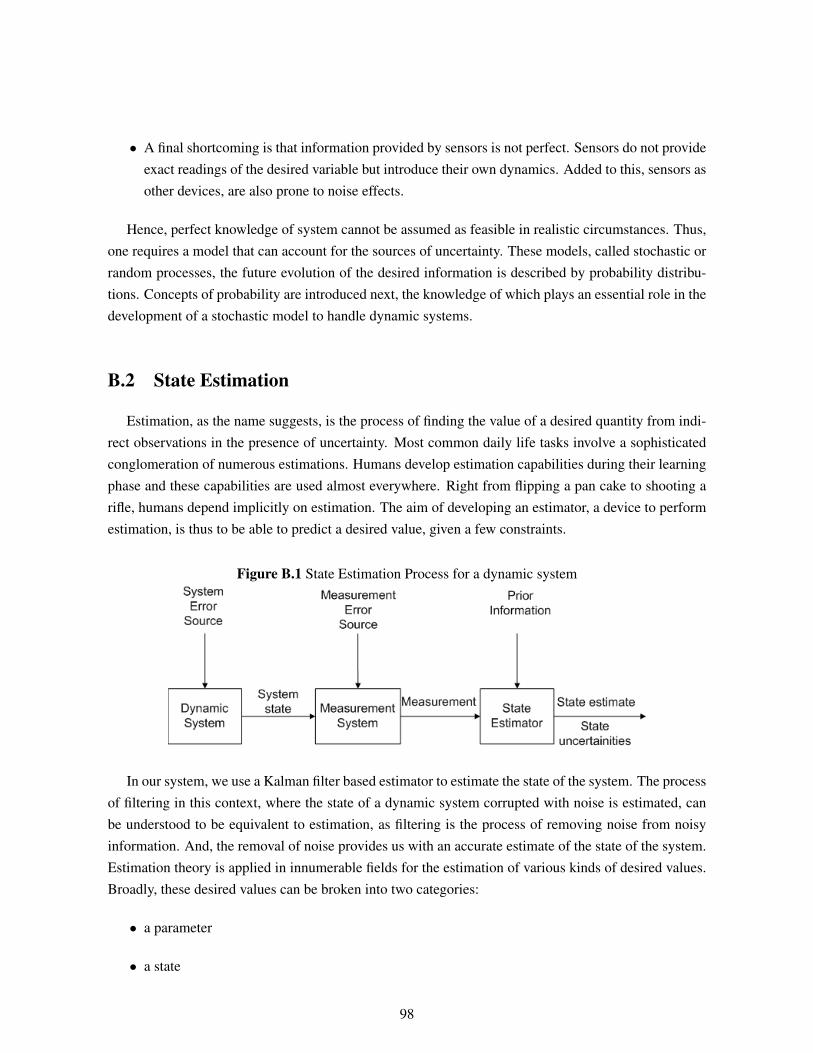
• A final shortcoming is that information provided by sensors is not perfect. Sensors do not provideexact readings of the desired variable but introduce their own dynamics. Added to this, sensors asother devices, are also prone to noise effects.

Hence, perfect knowledge of system cannot be assumed as feasible in realistic circumstances. Thus,one requires a model that can account for the sources of uncertainty. These models, called stochastic orrandom processes, the future evolution of the desired information is described by probability distribu-tions. Concepts of probability are introduced next, the knowledge of which plays an essential role in thedevelopment of a stochastic model to handle dynamic systems.

B.2 State Estimation

Estimation, as the name suggests, is the process of finding the value of a desired quantity from indi-rect observations in the presence of uncertainty. Most common daily life tasks involve a sophisticatedconglomeration of numerous estimations. Humans develop estimation capabilities during their learningphase and these capabilities are used almost everywhere. Right from flipping a pan cake to shooting arifle, humans depend implicitly on estimation. The aim of developing an estimator, a device to performestimation, is thus to be able to predict a desired value, given a few constraints.

Figure B.1 State Estimation Process for a dynamic system

In our system, we use a Kalman filter based estimator to estimate the state of the system. The processof filtering in this context, where the state of a dynamic system corrupted with noise is estimated, canbe understood to be equivalent to estimation, as filtering is the process of removing noise from noisyinformation. And, the removal of noise provides us with an accurate estimate of the state of the system.Estimation theory is applied in innumerable fields for the estimation of various kinds of desired values.Broadly, these desired values can be broken into two categories:

• a parameter

• a state

98

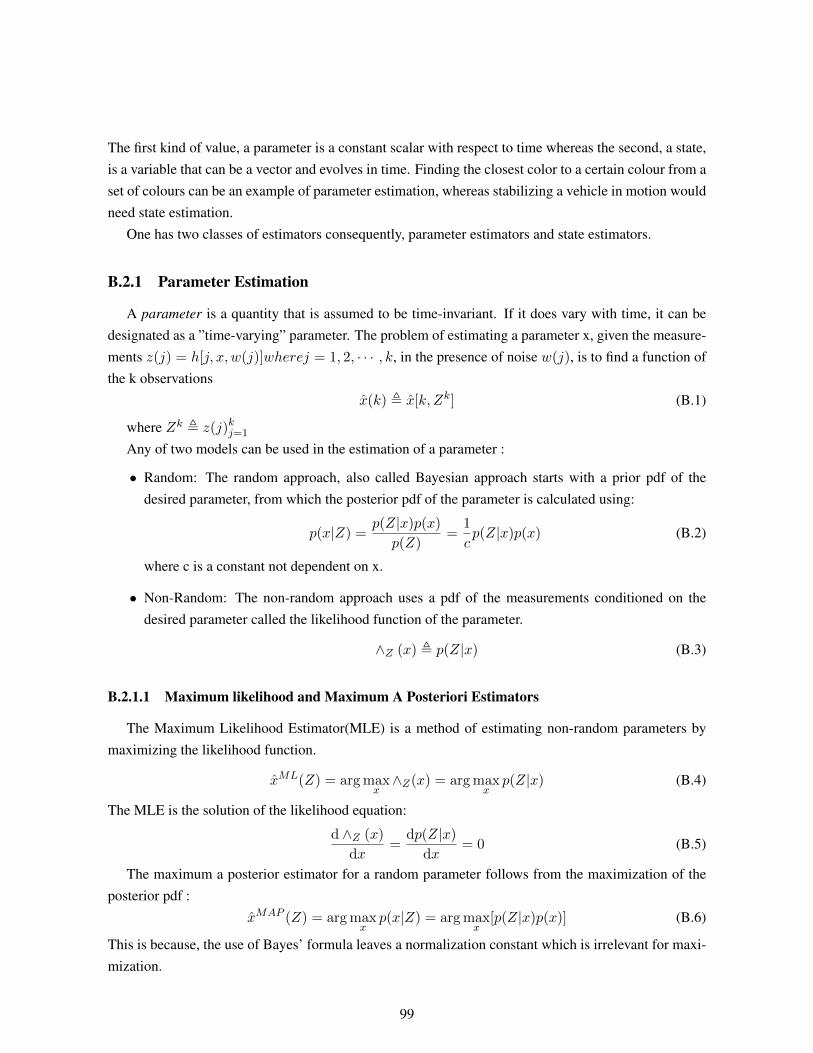
The first kind of value, a parameter is a constant scalar with respect to time whereas the second, a state,is a variable that can be a vector and evolves in time. Finding the closest color to a certain colour from aset of colours can be an example of parameter estimation, whereas stabilizing a vehicle in motion wouldneed state estimation.

One has two classes of estimators consequently, parameter estimators and state estimators.

B.2.1 Parameter Estimation

A parameter is a quantity that is assumed to be time-invariant. If it does vary with time, it can bedesignated as a ”time-varying” parameter. The problem of estimating a parameter x, given the measure-ments z(j) = h[j, x, w(j)]wherej = 1, 2, · · · , k, in the presence of noise w(j), is to find a function ofthe k observations

x(k) , x[k, Zk] (B.1)

where Zk , z(j)kj=1

Any of two models can be used in the estimation of a parameter :

• Random: The random approach, also called Bayesian approach starts with a prior pdf of thedesired parameter, from which the posterior pdf of the parameter is calculated using:

p(x|Z) =p(Z|x)p(x)

p(Z)=

1

cp(Z|x)p(x) (B.2)

where c is a constant not dependent on x.

• Non-Random: The non-random approach uses a pdf of the measurements conditioned on thedesired parameter called the likelihood function of the parameter.

∧Z (x) , p(Z|x) (B.3)

B.2.1.1 Maximum likelihood and Maximum A Posteriori Estimators

The Maximum Likelihood Estimator(MLE) is a method of estimating non-random parameters bymaximizing the likelihood function.

xML(Z) = arg maxx∧Z(x) = arg max

xp(Z|x) (B.4)

The MLE is the solution of the likelihood equation:

d ∧Z (x)

dx=

dp(Z|x)

dx= 0 (B.5)

The maximum a posterior estimator for a random parameter follows from the maximization of theposterior pdf :

xMAP (Z) = arg maxx

p(x|Z) = arg maxx

[p(Z|x)p(x)] (B.6)

This is because, the use of Bayes’ formula leaves a normalization constant which is irrelevant for maxi-mization.

99

B.2.1.2 Least Squares and Minimum Mean Square Error Estimators

The least squares method is q common procedure for the estimation of non-random parameters. Forthe measurements:

z(j) = h(j, x) + w(j)j = 1, 2, · · · , k (B.7)

the LSE of the non-random parameter x will be

xLS(k) = arg minx

k∑j=1

[z(j)− h(j, x)]2

(B.8)

Similarly, the MMSE for random parameters will be

xMMSE(Z) = E[x|Z] (B.9)

The above discussion assumes the estimation of a parameter, a constant variable only. However, tobuild a SLAM system, we need to estimate the location of the robot pose and the features. Obviously,the robot pose is not a constant as the robot traverses all over the map.

100