An EKF-SLAM toolbox in Matlab

Joan Sola – LAAS-CNRS

December 4, 2013

Contents

1 Quick start 31.1 Quick curiosity . . . . . . . . . . . . . . . . . . . . . . . . . . 31.2 Quick expert . . . . . . . . . . . . . . . . . . . . . . . . . . . 3

2 The SLAM toolbox presentation 5

3 Data organization 93.1 SLAM data . . . . . . . . . . . . . . . . . . . . . . . . . . . . 93.2 Simulation data . . . . . . . . . . . . . . . . . . . . . . . . . . 153.3 Graphics data . . . . . . . . . . . . . . . . . . . . . . . . . . . 183.4 Plain data . . . . . . . . . . . . . . . . . . . . . . . . . . . . . 22

4 Functions 234.1 High level . . . . . . . . . . . . . . . . . . . . . . . . . . . . . 234.2 Interface level . . . . . . . . . . . . . . . . . . . . . . . . . . . 254.3 Low level library . . . . . . . . . . . . . . . . . . . . . . . . . 27

5 Developing new observation models 285.1 Practical error-free procedure for the lazy-minded . . . . . . . 285.2 Steps to incorporate new models . . . . . . . . . . . . . . . . 295.3 Direct observation model for map corrections . . . . . . . . . 30

5.3.1 Build model from scratch . . . . . . . . . . . . . . . . 305.3.2 Adapting an existing model . . . . . . . . . . . . . . . 33

5.4 Inverse observation model for landmark initialization . . . . . 335.5 Landmark reparametrization . . . . . . . . . . . . . . . . . . 355.6 Landmark parameters out of the SLAM map . . . . . . . . . 365.7 Graphics . . . . . . . . . . . . . . . . . . . . . . . . . . . . . . 36

5.7.1 Graphic handles . . . . . . . . . . . . . . . . . . . . . 365.7.2 Graphic functions . . . . . . . . . . . . . . . . . . . . 37

1

6 Extensions 406.1 Extension with real images . . . . . . . . . . . . . . . . . . . 40

6.1.1 Loading, storing and displaying images . . . . . . . . . 406.1.2 Some image processing tools . . . . . . . . . . . . . . 416.1.3 The active-search algorithm . . . . . . . . . . . . . . . 42

7 Bibliography selection 46

2

1 Quick start

Hi there! To start the toolbox, do the following:

1. Visit www.joansola.eu and download the toolbox package.

2. Move slamToolbox.zip where you want the SLAM toolbox to beinstalled. Unzip it.

3. Rename the expanded directory if wanted (we’ll call this directorySLAMTB/).

4. Open Matlab. Add all directories and subdirectories in SLAMTB/ tothe Matlab path:File > Set Path > Add with subfolders > [select SLAMTB folder]

5. Go to the toolbox directory, cd [path]/SLAMTB/

6. Execute slamtb from the Matlab prompt.

1.1 Quick curiosity

Or, if you want to get some more insight:

7. Edit userData.m. Read the help lines. Explore options and create,by copying and modifying, new robots and sensors. You can modifythe robots’ initial positions and motions and the sensors’ positionsand parameters. You can also modify the default set of landmarks or‘World’.

8. Edit and run slamtb.m. Explore its code by debugging step-by-step.Explore the Map figure by zooming and rotating with the mouse.

9. Read the help contents of the following 4 functions: frame, fromFrame,q2R, pinHole. Follow some of the See also links.

10. Set FigOpt.createVideo to 'true' in userData. Obtain a series ofimages to create a video sequence – locate them atSLAMTB/figures/simu/idpPnt/mono/images/.

11. Read ‘guidelines.pdf’ before contributing your own code.

1.2 Quick expert

Or, if you want to explore the full capacity of this toolbox:

12. SLAM WITH POINTS: Choose userDataPnt instead of the de-fault userData (at the third line of code in slamtb.m). Scroll downto find the structure Obs. Try landmark types 'idpPnt', 'ahmPnt','hmgPnt', and 'fhmPnt'1 in entry Opt.init.initType, and com-

1Framed homogeneous points as described in [1]

3

pare performances of inverse-depth against anchored-homogeneous,framed-homogeneous and pure-homogeneous parametrizations for SLAMwith 3D points. Read [3, 16].

13. SLAM WITH LINES: Choose userDataLin instead of the defaultuserData (at the third line of code in slamtb.m). Scroll down tofind the structure Obs. Try landmark types 'plkLin', 'aplLin','hmgLin', 'ahmLin' and 'idpLin' in entry Opt.init.initTypeand compare performances of Plucker, anchored Plucker, Homoge-neous, Anchored-homogeneous and Inverse-depth parametrizations for3D lines. Read [17, 16].

14. SLAM WITH OMNIDIRECTIONAL CAMERA Edit userData.mor userDataPnt.m, go to the Sensor{1} section, comment it, anduncomment a second Sensor{1} below with a model for Omnicam.Choose 'ahmPnt' (see 12 above). Thanks to Grigory Abuladze forthis contribution!

15. SLAM WITH MULTIPLE SENSORS: Choose userData as theuser data file in slamtb. Uncomment the full Sensor{2} structure inuserData and get bi-camera SLAM. Set Sensor{2}.frameInMap to'true' and get extrinsic self-calibration of the stereo rig. Read [15].

16. SLAM WITH MULTIPLE ROBOTS: Uncomment the full Robot{2}structure. Set Sensor{2}.robot = 2 to assign sensor 2 to robot 2.Get multi-robot centralized SLAM. Read [15].

4

2 The SLAM toolbox presentation

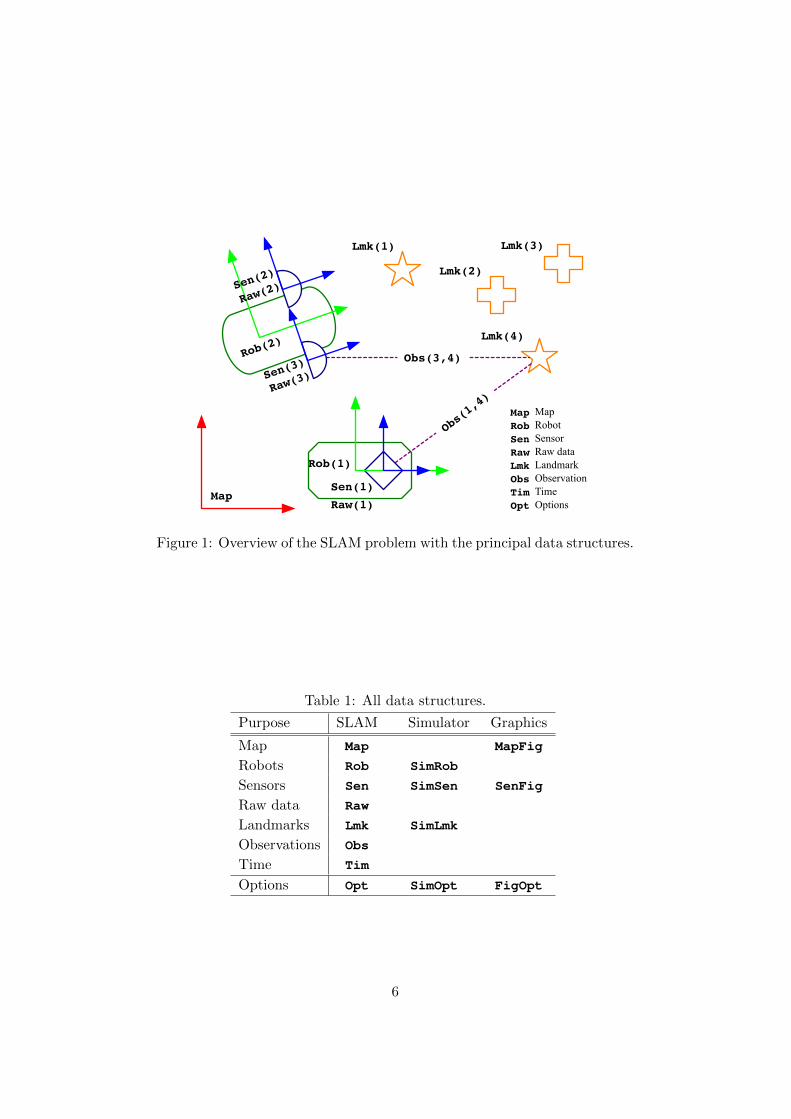
In a typical SLAM problem, one or more robots navigate an environment,discovering and mapping landmarks on the way by means of their onboardsensors. Observe in Fig. 1 the existence of robots of different kinds, carryinga different number of sensors of different kinds, which gather raw data and,by processing it, are capable of observing landmarks of different kinds. Allthis variety of data is handled by the present toolbox in a way that is quitetransparent.

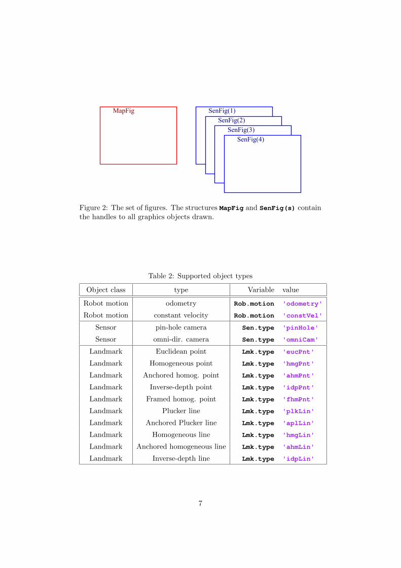
In this toolbox, we organized the data into three main groups, see Table1. The first group contains the objects of the SLAM problem itself, as theyappear in Fig. 1. A second group contains objects for simulation. A thirdgroup is designated for graphics output, Fig. 2. See Table 2 to see the objecttypes and options that are currently implemented.

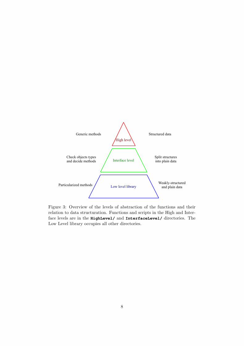
Apart from the data, we have of course the functions. Functions areorganized in three levels, from most abstract and generic to the basic ma-nipulations, as is sketched in Fig. 3. The highest level, called High Level,deals exclusively with the structured data we mentioned just above, and callsfunctions of an intermediate level called the Interface Level. The interfacelevel functions split the data structures into more mathematically meaning-ful elements, check objects types to decide on the applicable methods, andcall the basic functions that constitute the basic level, called the Low LevelLibrary.

5

Map

Lmk(1)

Lmk(4)

Lmk(2)

Lmk(3)

Opt OptionsTim Time

ObservationObs

Raw data

Map

Landmark

SensorSenRob RobotMap

LmkRaw

Obs(3,4)

Rob(1)

Sen(1)

Raw(1)

Obs(1,4)

Raw(3)

Rob(2)

Sen(2)

Sen(3)

Raw(2)

Figure 1: Overview of the SLAM problem with the principal data structures.

Table 1: All data structures.

Purpose SLAM Simulator Graphics

Map Map MapFig

Robots Rob SimRob

Sensors Sen SimSen SenFig

Raw data Raw

Landmarks Lmk SimLmk

Observations Obs

Time Tim

Options Opt SimOpt FigOpt

6

MapFig SenFig(1)SenFig(2)SenFig(3)SenFig(4)

Figure 2: The set of figures. The structures MapFig and SenFig(s) containthe handles to all graphics objects drawn.

Table 2: Supported object types

Object class type Variable value

Robot motion odometry Rob.motion 'odometry'

Robot motion constant velocity Rob.motion 'constVel'

Sensor pin-hole camera Sen.type 'pinHole'

Sensor omni-dir. camera Sen.type 'omniCam'

Landmark Euclidean point Lmk.type 'eucPnt'

Landmark Homogeneous point Lmk.type 'hmgPnt'

Landmark Anchored homog. point Lmk.type 'ahmPnt'

Landmark Inverse-depth point Lmk.type 'idpPnt'

Landmark Framed homog. point Lmk.type 'fhmPnt'

Landmark Plucker line Lmk.type 'plkLin'

Landmark Anchored Plucker line Lmk.type 'aplLin'

Landmark Homogeneous line Lmk.type 'hmgLin'

Landmark Anchored homogeneous line Lmk.type 'ahmLin'

Landmark Inverse-depth line Lmk.type 'idpLin'

7

Structured data

Split structures into plain data

Weakly-structured and plain data

Generic methods

Check objects types and decide methods

Particularized methods

High level

Low level library

Interface level

Figure 3: Overview of the levels of abstraction of the functions and theirrelation to data structuration. Functions and scripts in the High and Inter-face levels are in the HighLevel/ and InterfaceLevel/ directories. TheLow Level library occupies all other directories.

8

3 Data organization

It follows a brief explanation of the SLAM data structures, the Simulationand Graphic structures, and the plain data types.

3.1 SLAM data

For a SLAM system to be complete, we need to consider the following parts:

Rob: A set of robots.

Sen: A set of sensors.

Raw: A set of raw data captures, one per sensor.

Lmk: A set of landmarks.

Map: A stochastic map containing the states of robots, landmarks, andeventually sensors.

Obs: The set of landmark observations made by processing Raw data.

Tim: A few time-related variables.

Opt: Algorithm options.

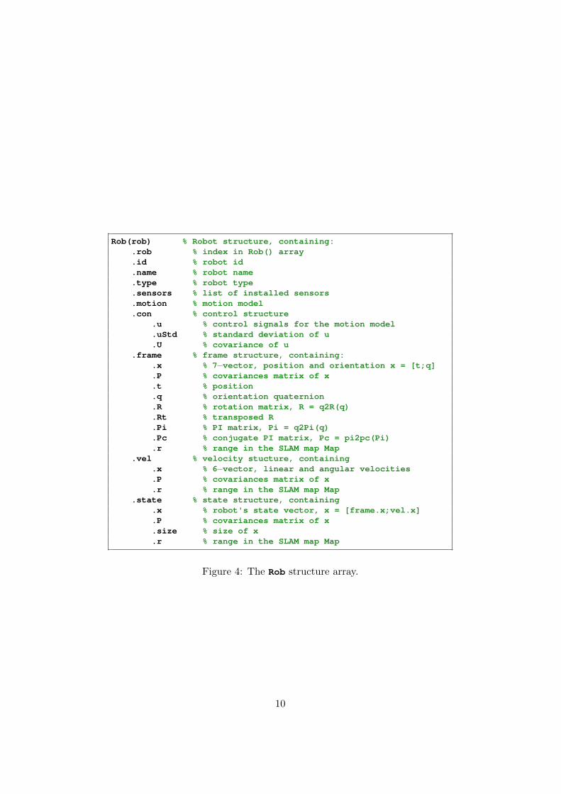
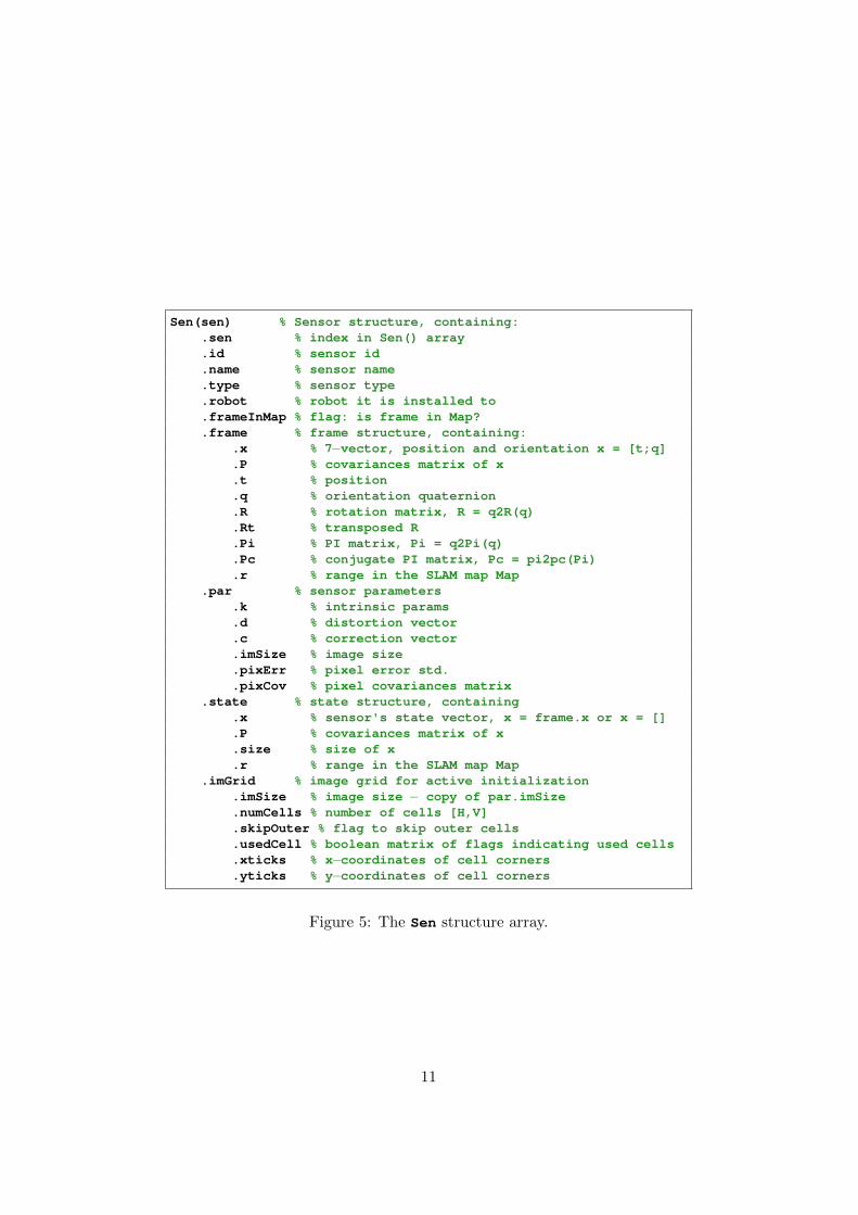
This toolbox considers these objects as the only existing data for SLAM.They are defined as structures holding a variety of fields (see Figs. 4 to11 for reference). Structure arrays hold any number of such objects. Forexample, all the data related to robot number 2 is stored in Rob(2). Toaccess the rotation matrix defining the orientation of this robot we simplyuse Rob(2).frame.R (type help frame at the Matlab prompt for help on3D reference frames). Observations require two indices because they relatesensors to landmarks. Thus, Obs(sen,lmk) stores the data associated tothe observation of landmark lmk from sensor sen.

It would be wise, before reading on, to revisit Fig. 1 and see how simplethings are.

It follows a reproduction of the arborescences of the principal structuresin the SLAM data.

9

Rob(rob) % Robot structure, containing:.rob % index in Rob() array.id % robot id.name % robot name.type % robot type.sensors % list of installed sensors.motion % motion model.con % control structure

.u % control signals for the motion model

.uStd % standard deviation of u

.U % covariance of u.frame % frame structure, containing:

.x % 7−vector, position and orientation x = [t;q]

.P % covariances matrix of x

.t % position

.q % orientation quaternion

.R % rotation matrix, R = q2R(q)

.Rt % transposed R

.Pi % PI matrix, Pi = q2Pi(q)

.Pc % conjugate PI matrix, Pc = pi2pc(Pi)

.r % range in the SLAM map Map.vel % velocity stucture, containing

.x % 6−vector, linear and angular velocities

.P % covariances matrix of x

.r % range in the SLAM map Map.state % state structure, containing

.x % robot's state vector, x = [frame.x;vel.x]

.P % covariances matrix of x

.size % size of x

.r % range in the SLAM map Map

Figure 4: The Rob structure array.

10

Sen(sen) % Sensor structure, containing:.sen % index in Sen() array.id % sensor id.name % sensor name.type % sensor type.robot % robot it is installed to.frameInMap % flag: is frame in Map?.frame % frame structure, containing:

.x % 7−vector, position and orientation x = [t;q]

.P % covariances matrix of x

.t % position

.q % orientation quaternion

.R % rotation matrix, R = q2R(q)

.Rt % transposed R

.Pi % PI matrix, Pi = q2Pi(q)

.Pc % conjugate PI matrix, Pc = pi2pc(Pi)

.r % range in the SLAM map Map.par % sensor parameters

.k % intrinsic params

.d % distortion vector

.c % correction vector

.imSize % image size

.pixErr % pixel error std.

.pixCov % pixel covariances matrix.state % state structure, containing

.x % sensor's state vector, x = frame.x or x = []

.P % covariances matrix of x

.size % size of x

.r % range in the SLAM map Map.imGrid % image grid for active initialization

.imSize % image size − copy of par.imSize

.numCells % number of cells [H,V]

.skipOuter % flag to skip outer cells

.usedCell % boolean matrix of flags indicating used cells

.xticks % x−coordinates of cell corners

.yticks % y−coordinates of cell corners

Figure 5: The Sen structure array.

11

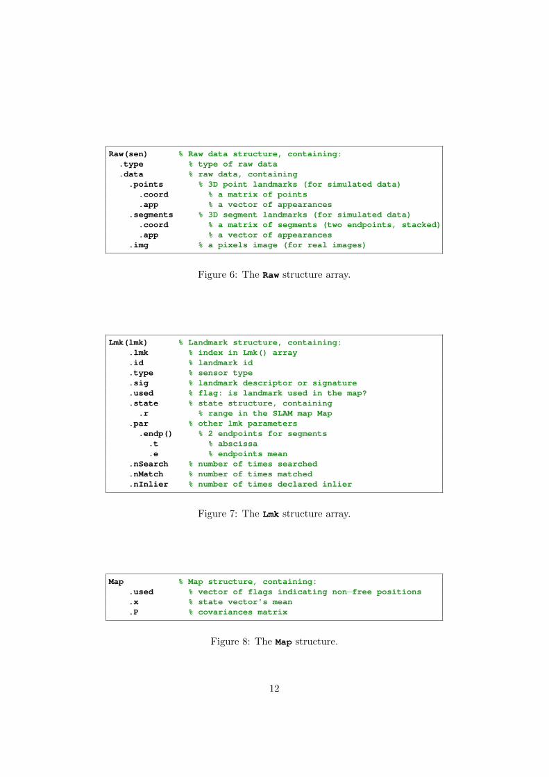
Raw(sen) % Raw data structure, containing:.type % type of raw data.data % raw data, containing

.points % 3D point landmarks (for simulated data).coord % a matrix of points.app % a vector of appearances

.segments % 3D segment landmarks (for simulated data).coord % a matrix of segments (two endpoints, stacked).app % a vector of appearances

.img % a pixels image (for real images)

Figure 6: The Raw structure array.

Lmk(lmk) % Landmark structure, containing:.lmk % index in Lmk() array.id % landmark id.type % sensor type.sig % landmark descriptor or signature.used % flag: is landmark used in the map?.state % state structure, containing.r % range in the SLAM map Map

.par % other lmk parameters.endp() % 2 endpoints for segments

.t % abscissa

.e % endpoints mean.nSearch % number of times searched.nMatch % number of times matched.nInlier % number of times declared inlier

Figure 7: The Lmk structure array.

Map % Map structure, containing:.used % vector of flags indicating non−free positions.x % state vector's mean.P % covariances matrix

Figure 8: The Map structure.

12

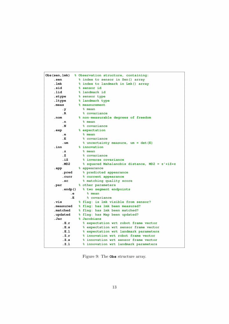
Obs(sen,lmk) % Observation structure, containing:.sen % index to sensor in Sen() array.lmk % index to landmark in Lmk() array.sid % sensor id.lid % landmark id.stype % sensor type.ltype % landmark type.meas % measurement

.y % mean

.R % covariance.nom % non−measurable degrees of freedom

.n % mean

.N % covariance.exp % expectation

.e % mean

.E % covariance

.um % uncertainty measure, um = det(E).inn % innovation

.z % mean

.Z % covariance

.iZ % inverse covariance

.MD2 % squared Mahalanobis distance, MD2 = z'*iZ*z.app % appearance

.pred % predicted appearance

.curr % current appearance

.sc % matching quality score.par % other parameters

.endp() % two segment endpoints.e % mean.E % covariance

.vis % flag: is lmk visible from sensor?

.measured % flag: has lmk been measured?

.matched % flag: has lmk been matched?

.updated % flag: has Map been updated?

.Jac % Jacobians.E r % expectation wrt robot frame vector.E s % expectation wrt sensor frame vector.E l % expectation wrt landmark parameters.Z r % innovation wrt robot frame vector.Z s % innovation wrt sensor frame vector.Z l % innovation wrt landmark parameters

Figure 9: The Obs structure array.

13

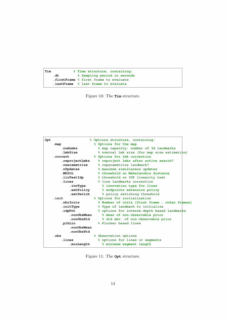
Tim % Time structure, containing:.dt % Sampling period in seconds.firstFrame % first frame to evaluate.lastFrame % last frame to evaluate

Figure 10: The Tim structure.

Opt % Options structure, containing:.map % Options for the map

.numLmks % map capacity: number of 3d landmarks

.lmkSize % nominal lmk size (for map size estimation).correct % Options for lmk correction

.reprojectLmks % reproject lmks after active search?

.rearametrize % reparametrize landmark?

.nUpdates % maximum simultaneus updates

.MD2th % threshold on Mahalanobis distance

.linTestIdp % threshold on IDP linearity test

.lines % line landmarks correction.innType % innovation type for lines.extPolicy % endpoints extension policy.extSwitch % policy switching threshold

.init % Options for initialization.nbrInits % Number of inits [first frame , other frames].initType % Type of landmark to initialize.idpPnt % options for inverse−depth based landmarks

.nonObsMean % mean of non−observable prior

.nonObsStd % std dev. of non−observable prior.plkLin % Plucker based lines

.nonObsMean

.nonObsStd.obs % Observation options

.lines % options for lines or segments.minLength % minimum segment length

Figure 11: The Opt structure.

14

3.2 Simulation data

This toolbox also includes simulated scenarios. We use for them the follow-ing objects, that come with 6-letter names to differentiate from the SLAMdata:

SimRob: Virtual robots for simulation.

SimSen: Virtual sensors for simulation.

SimLmk: A virtual world of landmarks for simulation.

SimOpt: Options for the simulator.

The simulation structures SimXxx are simplified versions of those existingin the SLAM data. Their arborescence is much smaller, and sometimes theymay have absolutely different organization. It is important to understandthat none of these structures is necessary if the toolbox is to be used withreal data.

It follows a reproduction of the arborescences of the principal simulationdata structures.

15

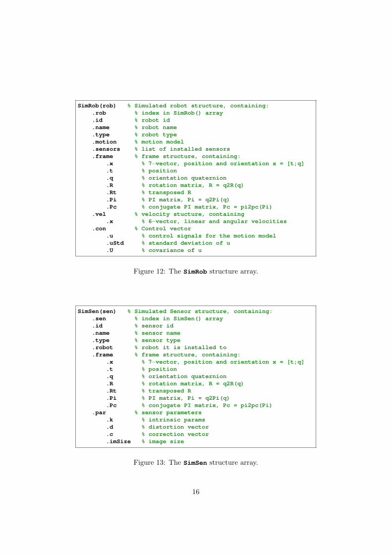
SimRob(rob) % Simulated robot structure, containing:.rob % index in SimRob() array.id % robot id.name % robot name.type % robot type.motion % motion model.sensors % list of installed sensors.frame % frame structure, containing:

.x % 7−vector, position and orientation x = [t;q]

.t % position

.q % orientation quaternion

.R % rotation matrix, R = q2R(q)

.Rt % transposed R

.Pi % PI matrix, Pi = q2Pi(q)

.Pc % conjugate PI matrix, Pc = pi2pc(Pi).vel % velocity stucture, containing

.x % 6−vector, linear and angular velocities.con % Control vector

.u % control signals for the motion model

.uStd % standard deviation of u

.U % covariance of u

Figure 12: The SimRob structure array.

SimSen(sen) % Simulated Sensor structure, containing:.sen % index in SimSen() array.id % sensor id.name % sensor name.type % sensor type.robot % robot it is installed to.frame % frame structure, containing:

.x % 7−vector, position and orientation x = [t;q]

.t % position

.q % orientation quaternion

.R % rotation matrix, R = q2R(q)

.Rt % transposed R

.Pi % PI matrix, Pi = q2Pi(q)

.Pc % conjugate PI matrix, Pc = pi2pc(Pi).par % sensor parameters

.k % intrinsic params

.d % distortion vector

.c % correction vector

.imSize % image size

Figure 13: The SimSen structure array.

16

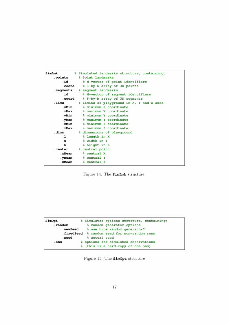
SimLmk % Simulated landmarks structure, containing:.points % Point landmarks

.id % N−vector of point identifiers

.coord % 3−by−N array of 3D points.segments % segment landmarks

.id % M−vector of segment identifiers

.coord % 6−by−M array of 3D segments.lims % limits of playground in X, Y and Z axes

.xMin % minimum X coordinate

.xMax % maximum X coordinate

.yMin % minimum Y coordinate

.yMax % maximum Y coordinate

.zMin % minimum Z coordinate

.zMax % maximum Z coordinate.dims % dimensions of playground

.l % length in X

.w % width in Y

.h % height in Z.center % central point

.xMean % central X

.yMean % central Y

.zMean % central Z

Figure 14: The SimLmk structure.

SimOpt % Simulator options structure, containing:.random % random generator options

.newSeed % use true random generator?

.fixedSeed % random seed for non−random runs

.seed % actual seed.obs % options for simulated observations.

% (this is a hard−copy of Obs.obs)

Figure 15: The SimOpt structure

17

3.3 Graphics data

This toolbox also includes graphics output. We use for them the followingobjects, which come also with 6-letter names:

MapFig: A structure of handles to graphics objects in the 3D map figure.One Map figure showing the world, the robots, the sensors, and thecurrent state of the estimated SLAM map (Figs. 16 and 17).

SenFig: A structure array of handles to graphics objects in the sensorfigures. One figure per sensor, visualizing its measurement space (Figs.18 and 19).

FigOpt: A structure with options for figures such as colors, views andprojections.

It follows a reproduction of the arborescences of the principal graphicsstructures. See Section 5.7 for information about graphic functions.

18

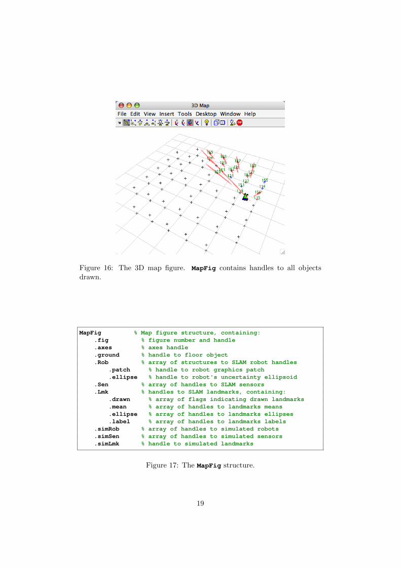
Figure 16: The 3D map figure. MapFig contains handles to all objectsdrawn.

MapFig % Map figure structure, containing:.fig % figure number and handle.axes % axes handle.ground % handle to floor object.Rob % array of structures to SLAM robot handles

.patch % handle to robot graphics patch

.ellipse % handle to robot's uncertainty ellipsoid.Sen % array of handles to SLAM sensors.Lmk % handles to SLAM landmarks, containing:

.drawn % array of flags indicating drawn landmarks

.mean % array of handles to landmarks means

.ellipse % array of handles to landmarks ellipses

.label % array of handles to landmarks labels.simRob % array of handles to simulated robots.simSen % array of handles to simulated sensors.simLmk % handle to simulated landmarks

Figure 17: The MapFig structure.

19

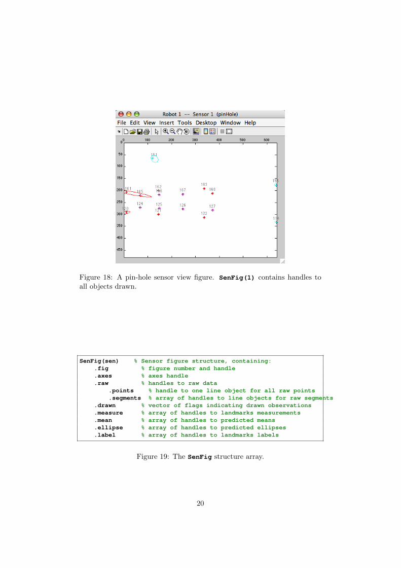
Figure 18: A pin-hole sensor view figure. SenFig(1) contains handles toall objects drawn.

SenFig(sen) % Sensor figure structure, containing:.fig % figure number and handle.axes % axes handle.raw % handles to raw data

.points % handle to one line object for all raw points

.segments % array of handles to line objects for raw segments.drawn % vector of flags indicating drawn observations.measure % array of handles to landmarks measurements.mean % array of handles to predicted means.ellipse % array of handles to predicted ellipses.label % array of handles to landmarks labels

Figure 19: The SenFig structure array.

20

FigOpt % Figure options structure, containing:.renderer % renderer.rendPeriod % rendering period in frames.createVideo % flag: create video sequence?.map % map figure options

.proj % projection of the 3d figure

.view % viewpoint of the 3d figure

.orbit % AZ and EL orbit angle increments

.size % map figure size

.showSimLmk % flag: show simulated landmarks?

.showEllip % flag: show uncertainty ellipsoids?

.colors % map figure colors.border % border.axes % axes, ticks and axes labels.bckgnd % background.simLmk % simulated landmarks.defPnt % default point

.mean % mean dot

.ellip % ellipsoid.othPnt % other point

.mean % mean dot

.ellip % ellipsoid.defLin % default line

.mean % mean line

.ellip % endpoint ellipsoids.simu % simulated robots and sensors.est % estimated robots and sensors.ground % ground.label % landmark ID labels

.sensor % sensor figures options.size % sensor figure size.showEllip % flag: show uncertainty ellipses?.colors % Sensor figure colors:.border % border.axes % axes, ticks and axes labels.bckgnd % background.raw % raw data.defPnt % euclidean point

.updated % updated

.predicted % predicted.othPnt % other point

.updated % updated

.predicted % predicted.defLin % default line

.meas % measurement

.mean % mean line

.ellip % endpoint ellipses.othLin % other line

.meas % measurement

.mean % mean line

.ellip % endpoint ellipses.label % label

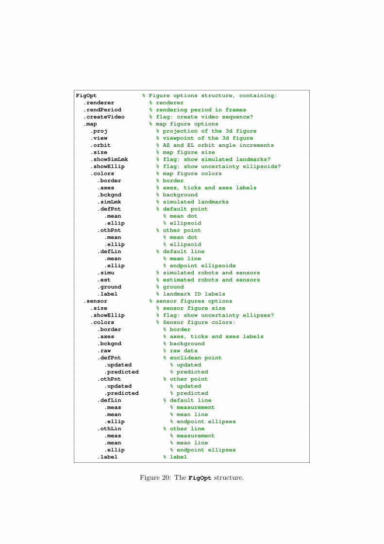
Figure 20: The FigOpt structure.

3.4 Plain data

The structured data we have seen so far is composed of chunks of lowercomplexity structures and plain data. This plain data is the data that thelow-level functions take as inputs and deliver as outputs.

For plain data we mean:

logicals and scalars: Any Matlab scalar value such as a = 5 or b = true.

vectors and matrices: Any Matlab array such as v = [1;2], w = [1 2],c = [true false] or M = [1 2;3 4].

character strings: Any Matlab alphanumeric string such as type = 'pinHole'or dir = '%HOME/tmp/'.

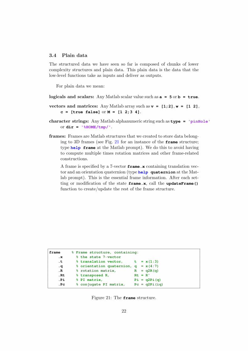
frames: Frames are Matlab structures that we created to store data belong-ing to 3D frames (see Fig. 21 for an instance of the frame structure;type help frame at the Matlab prompt). We do this to avoid havingto compute multiple times rotation matrices and other frame-relatedconstructions.

A frame is specified by a 7-vector frame.x containing translation vec-tor and an orientation quaternion (type help quaternion at the Mat-lab prompt). This is the essential frame information. After each set-ting or modification of the state frame.x, call the updateFrame()function to create/update the rest of the frame structure.

frame % Frame structure, containing:.x % the state 7−vector.t % translation vector, t = x(1:3).q % orientation quaternion, q = x(4:7).R % rotation matrix, R = q2R(q).Rt % transposed R, Rt = R'.Pi % PI matrix, Pi = q2Pi(q).Pc % conjugate PI matrix, Pc = q2Pi(iq)

Figure 21: The frame structure.

22

4 Functions

The SLAM toolbox is composed of functions of different importance, defin-ing three levels of abstraction (Fig. 3). They are stored in subdirectoriesaccording to their field of utility. There are two particular directories:HighLevel, with two scripts and a limited set of high-level functions; andInterfaceLevel, with a number of functions interfacing the high level datawith the low-level library. All other directories contain low-level functions.

4.1 High level

The high level scripts and functions are located in the directorySLAMtoolbox/HighLevel/.

There are two main scripts that constitute the highest level, one for thecode and one for the data:

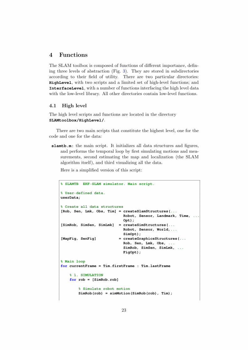
slamtb.m: the main script. It initializes all data structures and figures,and performs the temporal loop by first simulating motions and mea-surements, second estimating the map and localization (the SLAMalgorithm itself), and third visualizing all the data.

Here is a simplified version of this script:

% SLAMTB EKF−SLAM simulator. Main script.

% User−defined data.userData;

% Create all data structures[Rob, Sen, Lmk, Obs, Tim] = createSlamStructures(...

Robot, Sensor, Landmark, Time, ...Opt);

[SimRob, SimSen, SimLmk] = createSimStructures(...Robot, Sensor, World,...SimOpt);

[MapFig, SenFig] = createGraphicsStructures(...Rob, Sen, Lmk, Obs, ...SimRob, SimSen, SimLmk, ...FigOpt);

% Main loopfor currentFrame = Tim.firstFrame : Tim.lastFrame

% 1. SIMULATIONfor rob = [SimRob.rob]

% Simulate robot motionSimRob(rob) = simMotion(SimRob(rob), Tim);

23

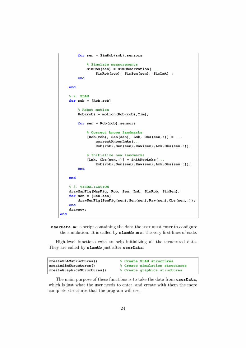
for sen = SimRob(rob).sensors

% Simulate measurementsSimObs(sen) = simObservation(...

SimRob(rob), SimSen(sen), SimLmk) ;end

end

% 2. SLAMfor rob = [Rob.rob]

% Robot motionRob(rob) = motion(Rob(rob),Tim);

for sen = Rob(rob).sensors

% Correct known landmarks[Rob(rob), Sen(sen), Lmk, Obs(sen,:)] = ...

correctKnownLmks(...Rob(rob),Sen(sen),Raw(sen),Lmk,Obs(sen,:));

% Initialize new landmarks[Lmk, Obs(sen,:)] = initNewLmks(...

Rob(rob),Sen(sen),Raw(sen),Lmk,Obs(sen,:));end

end

% 3. VISUALIZATIONdrawMapFig(MapFig, Rob, Sen, Lmk, SimRob, SimSen);for sen = [Sen.sen]

drawSenFig(SenFig(sen),Sen(sen),Raw(sen),Obs(sen,:));enddrawnow;

end

userData.m: a script containing the data the user must enter to configurethe simulation. It is called by slamtb.m at the very first lines of code.

High-level functions exist to help initializing all the structured data.They are called by slamtb just after userData:

createSLAMstructures() % Create SLAM structurescreateSimStructures() % Create simulation structurescreateGraphicsStructures() % Create graphics structures

The main purpose of these functions is to take the data from userData,which is just what the user needs to enter, and create with them the morecomplete structures that the program will use.

24

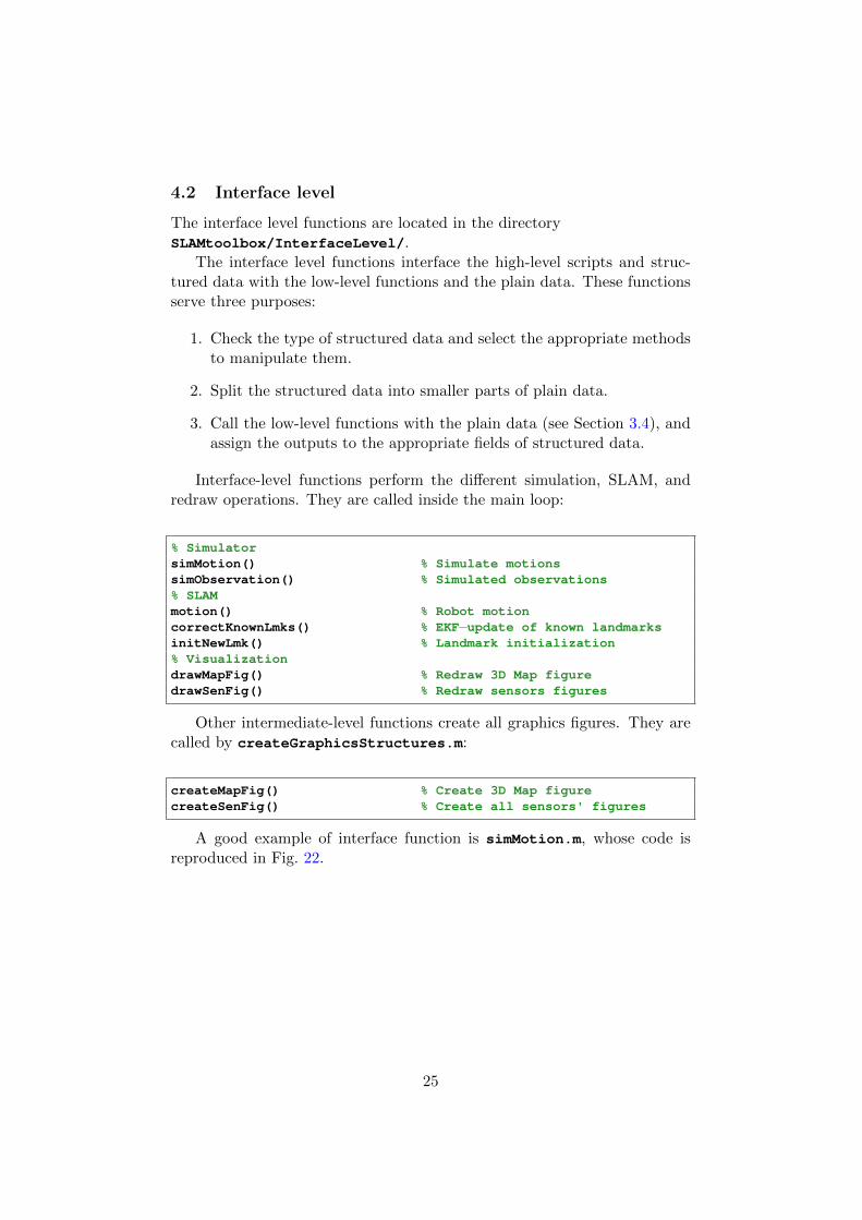
4.2 Interface level

The interface level functions are located in the directorySLAMtoolbox/InterfaceLevel/.

The interface level functions interface the high-level scripts and struc-tured data with the low-level functions and the plain data. These functionsserve three purposes:

1. Check the type of structured data and select the appropriate methodsto manipulate them.

2. Split the structured data into smaller parts of plain data.

3. Call the low-level functions with the plain data (see Section 3.4), andassign the outputs to the appropriate fields of structured data.

Interface-level functions perform the different simulation, SLAM, andredraw operations. They are called inside the main loop:

% SimulatorsimMotion() % Simulate motionssimObservation() % Simulated observations% SLAMmotion() % Robot motioncorrectKnownLmks() % EKF−update of known landmarksinitNewLmk() % Landmark initialization% VisualizationdrawMapFig() % Redraw 3D Map figuredrawSenFig() % Redraw sensors figures

Other intermediate-level functions create all graphics figures. They arecalled by createGraphicsStructures.m:

createMapFig() % Create 3D Map figurecreateSenFig() % Create all sensors' figures

A good example of interface function is simMotion.m, whose code isreproduced in Fig. 22.

25

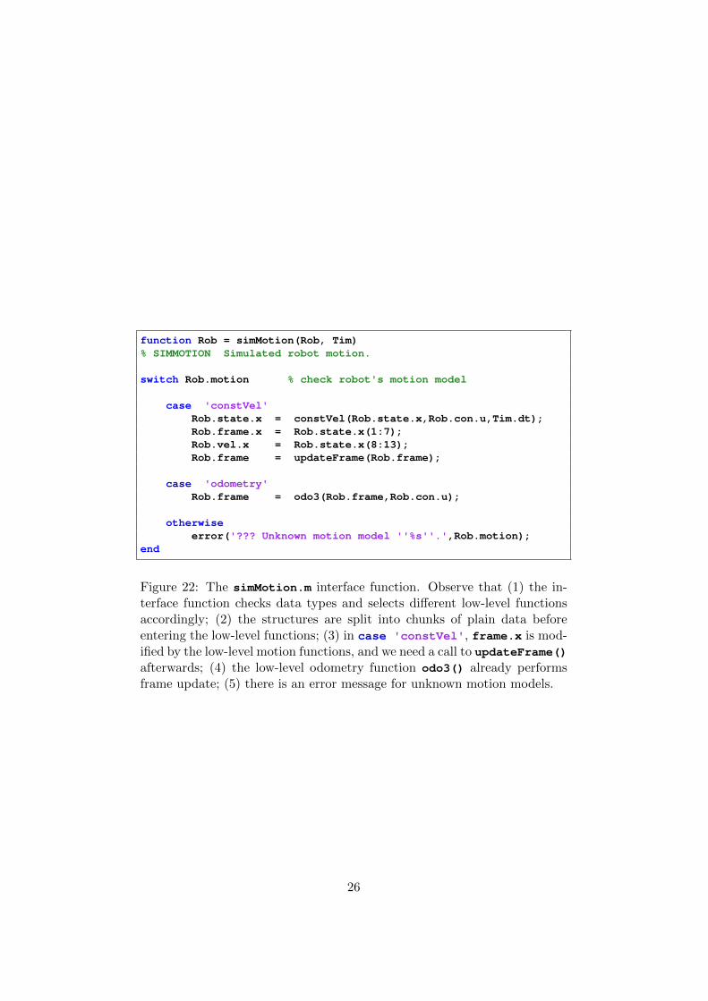
function Rob = simMotion(Rob, Tim)% SIMMOTION Simulated robot motion.

switch Rob.motion % check robot's motion model

case 'constVel'Rob.state.x = constVel(Rob.state.x,Rob.con.u,Tim.dt);Rob.frame.x = Rob.state.x(1:7);Rob.vel.x = Rob.state.x(8:13);Rob.frame = updateFrame(Rob.frame);

case 'odometry'Rob.frame = odo3(Rob.frame,Rob.con.u);

otherwiseerror('??? Unknown motion model ''%s''.',Rob.motion);

end

Figure 22: The simMotion.m interface function. Observe that (1) the in-terface function checks data types and selects different low-level functionsaccordingly; (2) the structures are split into chunks of plain data beforeentering the low-level functions; (3) in case 'constVel', frame.x is mod-ified by the low-level motion functions, and we need a call to updateFrame()afterwards; (4) the low-level odometry function odo3() already performsframe update; (5) there is an error message for unknown motion models.

26

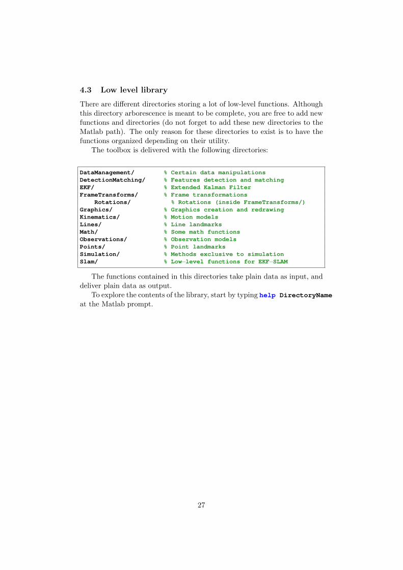
4.3 Low level library

There are different directories storing a lot of low-level functions. Althoughthis directory arborescence is meant to be complete, you are free to add newfunctions and directories (do not forget to add these new directories to theMatlab path). The only reason for these directories to exist is to have thefunctions organized depending on their utility.

The toolbox is delivered with the following directories:

DataManagement/ % Certain data manipulationsDetectionMatching/ % Features detection and matchingEKF/ % Extended Kalman FilterFrameTransforms/ % Frame transformations

Rotations/ % Rotations (inside FrameTransforms/)Graphics/ % Graphics creation and redrawingKinematics/ % Motion modelsLines/ % Line landmarksMath/ % Some math functionsObservations/ % Observation modelsPoints/ % Point landmarksSimulation/ % Methods exclusive to simulationSlam/ % Low−level functions for EKF−SLAM

The functions contained in this directories take plain data as input, anddeliver plain data as output.

To explore the contents of the library, start by typing help DirectoryNameat the Matlab prompt.

27

5 Developing new observation models

This section describes the necessary steps for creating new observation mod-els any time a new type of sensor and/or a new type of landmark is consid-ered. Please read ‘guidelines.pdf’ before contributing your own code.

Before you develop a new observation model, you must take care of thefollowing facts:

1. You need a direct observation model for observing known landmarksand correcting the map, and an inverse observation model for land-mark initialization.

2. The robot acts as a mere support for sensors. Normally, only itscurrent frame is of any interest. In some (rare) special cases, therobot’s velocity may be of interest if the measurements are sensitiveto it (for example, when considering a sonar sensor with Doppler-effectcapabilities).

3. The sensor’s frame is specified in robot frame. It may be part of theSLAM state vector.

4. The sensor contains other parameters. The number and nature of theseparameters depend on the type of sensor and cannot be generalized.We have not considered these parameters as part of the SLAM statevector, although this could be done. Most observation functions in thetoolbox already return the Jacobians with respect to these parameters.

5. The landmark has the main parameters in the SLAM vector, but itmay have some other parameters out of it.

6. The sensor may provide full or partial measurements of the landmarkstate. In case of partial measurements, you have to provide a Gaussianprior of the non-measured part for initialization.

5.1 Practical error-free procedure for the lazy-minded

To start the creation of a new model, simply edit userData.m and enter anew string in Opt.init.initType (for example, enter the string 'newLin'to create a new line. When creating a new landmark model, remember touse strictly 6 characters, with the last 3 indicating either 'Pnt' or 'Lin'!.Then execute slamtb. The program will fail exactly in the place where youneed to enter new code. Let me call this an entry point. Read the errorcomment and check the existing code close to the entry point: get inspiredon it and you will soon know what to do, and how to do it. After addingthe code (and saving the corresponding file!), re-execute slamtb to advanceto the next entry point.

28

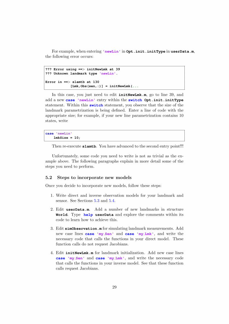
For example, when entering 'newLin' in Opt.init.initType in userData.m,the following error occurs:

??? Error using ==> initNewLmk at 39??? Unknown landmark type 'newLin'.

Error in ==> slamtb at 130[Lmk,Obs(sen,:)] = initNewLmk(...

In this case, you just need to edit initNewLmk.m, go to line 39, andadd a new case 'newLin' entry within the switch Opt.init.initTypestatement. Within this switch statement, you observe that the size of thelandmark parametrization is being defined. Enter a line of code with theappropriate size; for example, if your new line parametrization contains 10states, write

case 'newLin'lmkSize = 10;

Then re-execute slamtb. You have advanced to the second entry point!!!

Unfortunately, some code you need to write is not as trivial as the ex-ample above. The following paragraphs explain in more detail some of thesteps you need to perform.

5.2 Steps to incorporate new models

Once you decide to incorporate new models, follow these steps:

1. Write direct and inverse observation models for your landmark andsensor. See Sections 5.3 and 5.4.

2. Edit userData.m. Add a number of new landmarks in structureWorld. Type help userData and explore the comments within itscode to learn how to achieve this.

3. Edit simObservation.m for simulating landmark measurements. Addnew case lines case 'my Sen' and case 'my Lmk', and write thenecessary code that calls the functions in your direct model. Thesefunction calls do not request Jacobians.

4. Edit initNewLmk.m for landmark initialization. Add new case linescase 'my Sen' and case 'my Lmk', and write the necessary codethat calls the functions in your inverse model. See that these functioncalls request Jacobians.

29

5. Edit correctKnownLmks.m for landmark corrections. Add new caselines case 'my Sen' and case 'my Lmk', and write the necessarycode that calls the functions in your direct model. See that thesefunction calls request Jacobians. Name the return variable and Jaco-bians exactly as in the other existing models: they are used later. SeeSections 5.3, 5.5 and 5.6.

6. Edit createMapFig.m and createSenFig.m for map and sensor fig-ures. Add new switch−case entries and the methods to create thedesired graphics. See Section 5.7.

7. Edit drawMapFig.m and drawSenFig.m to redraw the new landmarksin the map and sensor figures. Add new switch−case entries andcreate the desired methods for showing the landmarks and associatedobservations. See Section 5.7.

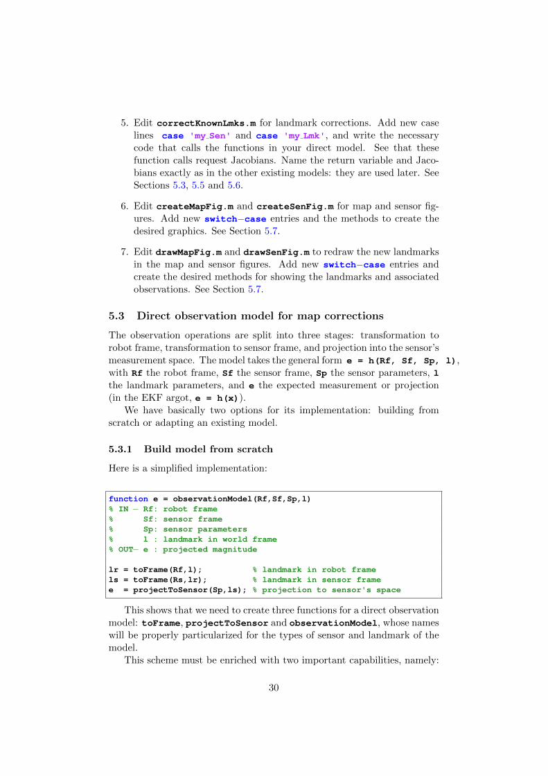
5.3 Direct observation model for map corrections

The observation operations are split into three stages: transformation torobot frame, transformation to sensor frame, and projection into the sensor’smeasurement space. The model takes the general form e = h(Rf, Sf, Sp, l),with Rf the robot frame, Sf the sensor frame, Sp the sensor parameters, lthe landmark parameters, and e the expected measurement or projection(in the EKF argot, e = h(x)).

We have basically two options for its implementation: building fromscratch or adapting an existing model.

5.3.1 Build model from scratch

Here is a simplified implementation:

function e = observationModel(Rf,Sf,Sp,l)% IN − Rf: robot frame% Sf: sensor frame% Sp: sensor parameters% l : landmark in world frame% OUT− e : projected magnitude

lr = toFrame(Rf,l); % landmark in robot framels = toFrame(Rs,lr); % landmark in sensor framee = projectToSensor(Sp,ls); % projection to sensor's space

This shows that we need to create three functions for a direct observationmodel: toFrame, projectToSensor and observationModel, whose nameswill be properly particularized for the types of sensor and landmark of themodel.

This scheme must be enriched with two important capabilities, namely:

30

• Jacobian matrices computation.

• Vectorized operation for multiple landmarks.

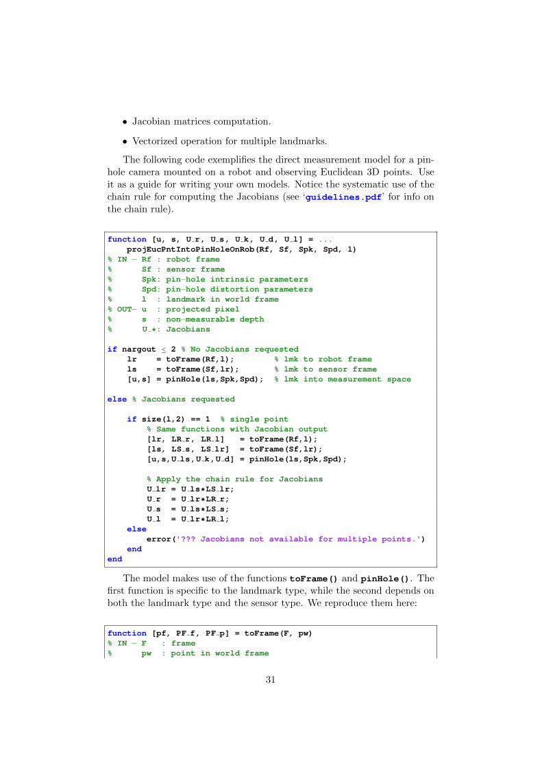
The following code exemplifies the direct measurement model for a pin-hole camera mounted on a robot and observing Euclidean 3D points. Useit as a guide for writing your own models. Notice the systematic use of thechain rule for computing the Jacobians (see ‘guidelines.pdf’ for info onthe chain rule).

function [u, s, U r, U s, U k, U d, U l] = ...projEucPntIntoPinHoleOnRob(Rf, Sf, Spk, Spd, l)

% IN − Rf : robot frame% Sf : sensor frame% Spk: pin−hole intrinsic parameters% Spd: pin−hole distortion parameters% l : landmark in world frame% OUT− u : projected pixel% s : non−measurable depth% U *: Jacobians

if nargout ≤ 2 % No Jacobians requestedlr = toFrame(Rf,l); % lmk to robot framels = toFrame(Sf,lr); % lmk to sensor frame[u,s] = pinHole(ls,Spk,Spd); % lmk into measurement space

else % Jacobians requested

if size(l,2) == 1 % single point% Same functions with Jacobian output[lr, LR r, LR l] = toFrame(Rf,l);[ls, LS s, LS lr] = toFrame(Sf,lr);[u,s,U ls,U k,U d] = pinHole(ls,Spk,Spd);

% Apply the chain rule for JacobiansU lr = U ls*LS lr;U r = U lr*LR r;U s = U ls*LS s;U l = U lr*LR l;

elseerror('??? Jacobians not available for multiple points.')

endend

The model makes use of the functions toFrame() and pinHole(). Thefirst function is specific to the landmark type, while the second depends onboth the landmark type and the sensor type. We reproduce them here:

function [pf, PF f, PF p] = toFrame(F, pw)% IN − F : frame% pw : point in world frame

31

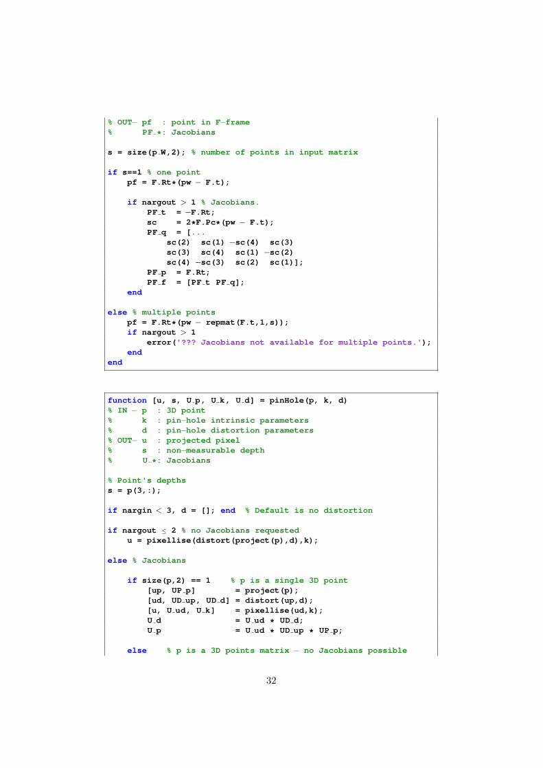
% OUT− pf : point in F−frame% PF *: Jacobians

s = size(p W,2); % number of points in input matrix

if s==1 % one pointpf = F.Rt*(pw − F.t);

if nargout > 1 % Jacobians.PF t = −F.Rt;sc = 2*F.Pc*(pw − F.t);PF q = [...

sc(2) sc(1) −sc(4) sc(3)sc(3) sc(4) sc(1) −sc(2)sc(4) −sc(3) sc(2) sc(1)];

PF p = F.Rt;PF f = [PF t PF q];

end

else % multiple pointspf = F.Rt*(pw − repmat(F.t,1,s));if nargout > 1

error('??? Jacobians not available for multiple points.');end

end

function [u, s, U p, U k, U d] = pinHole(p, k, d)% IN − p : 3D point% k : pin−hole intrinsic parameters% d : pin−hole distortion parameters% OUT− u : projected pixel% s : non−measurable depth% U *: Jacobians

% Point's depthss = p(3,:);

if nargin < 3, d = []; end % Default is no distortion

if nargout ≤ 2 % no Jacobians requestedu = pixellise(distort(project(p),d),k);

else % Jacobians

if size(p,2) == 1 % p is a single 3D point[up, UP p] = project(p);[ud, UD up, UD d] = distort(up,d);[u, U ud, U k] = pixellise(ud,k);U d = U ud * UD d;U p = U ud * UD up * UP p;

else % p is a 3D points matrix − no Jacobians possible

32

error('??? Jacobians not available for multiple points.')end

end

5.3.2 Adapting an existing model

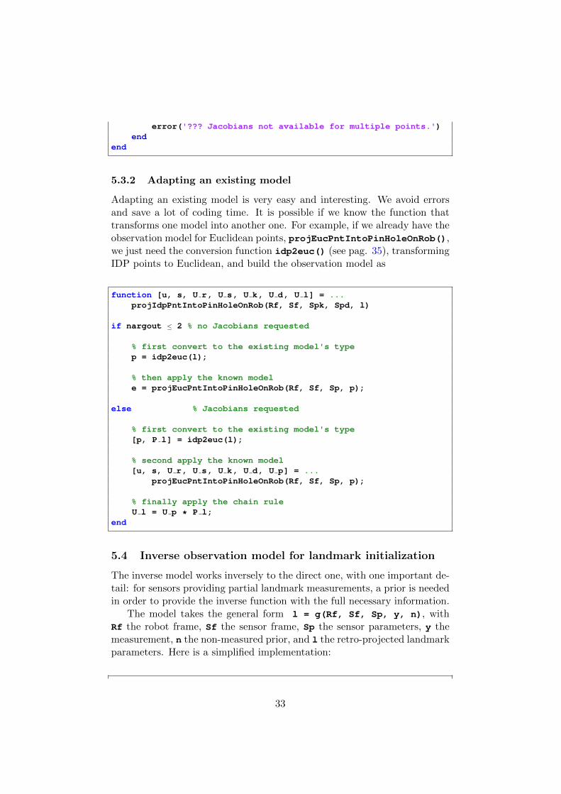
Adapting an existing model is very easy and interesting. We avoid errorsand save a lot of coding time. It is possible if we know the function thattransforms one model into another one. For example, if we already have theobservation model for Euclidean points, projEucPntIntoPinHoleOnRob(),we just need the conversion function idp2euc() (see pag. 35), transformingIDP points to Euclidean, and build the observation model as

function [u, s, U r, U s, U k, U d, U l] = ...projIdpPntIntoPinHoleOnRob(Rf, Sf, Spk, Spd, l)

if nargout ≤ 2 % no Jacobians requested

% first convert to the existing model's typep = idp2euc(l);

% then apply the known modele = projEucPntIntoPinHoleOnRob(Rf, Sf, Sp, p);

else % Jacobians requested

% first convert to the existing model's type[p, P l] = idp2euc(l);

% second apply the known model[u, s, U r, U s, U k, U d, U p] = ...

projEucPntIntoPinHoleOnRob(Rf, Sf, Sp, p);

% finally apply the chain ruleU l = U p * P l;

end

5.4 Inverse observation model for landmark initialization

The inverse model works inversely to the direct one, with one important de-tail: for sensors providing partial landmark measurements, a prior is neededin order to provide the inverse function with the full necessary information.

The model takes the general form l = g(Rf, Sf, Sp, y, n), withRf the robot frame, Sf the sensor frame, Sp the sensor parameters, y themeasurement, n the non-measured prior, and l the retro-projected landmarkparameters. Here is a simplified implementation:

33

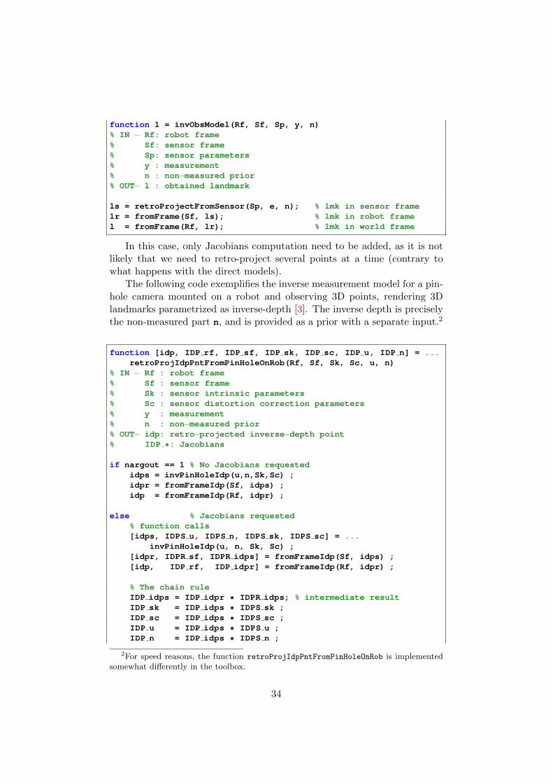
function l = invObsModel(Rf, Sf, Sp, y, n)% IN − Rf: robot frame% Sf: sensor frame% Sp: sensor parameters% y : measurement% n : non−measured prior% OUT− l : obtained landmark

ls = retroProjectFromSensor(Sp, e, n); % lmk in sensor framelr = fromFrame(Sf, ls); % lmk in robot framel = fromFrame(Rf, lr); % lmk in world frame

In this case, only Jacobians computation need to be added, as it is notlikely that we need to retro-project several points at a time (contrary towhat happens with the direct models).

The following code exemplifies the inverse measurement model for a pin-hole camera mounted on a robot and observing 3D points, rendering 3Dlandmarks parametrized as inverse-depth [3]. The inverse depth is preciselythe non-measured part n, and is provided as a prior with a separate input.2

function [idp, IDP rf, IDP sf, IDP sk, IDP sc, IDP u, IDP n] = ...retroProjIdpPntFromPinHoleOnRob(Rf, Sf, Sk, Sc, u, n)

% IN − Rf : robot frame% Sf : sensor frame% Sk : sensor intrinsic parameters% Sc : sensor distortion correction parameters% y : measurement% n : non−measured prior% OUT− idp: retro−projected inverse−depth point% IDP *: Jacobians

if nargout == 1 % No Jacobians requestedidps = invPinHoleIdp(u,n,Sk,Sc) ;idpr = fromFrameIdp(Sf, idps) ;idp = fromFrameIdp(Rf, idpr) ;

else % Jacobians requested% function calls[idps, IDPS u, IDPS n, IDPS sk, IDPS sc] = ...

invPinHoleIdp(u, n, Sk, Sc) ;[idpr, IDPR sf, IDPR idps] = fromFrameIdp(Sf, idps) ;[idp, IDP rf, IDP idpr] = fromFrameIdp(Rf, idpr) ;

% The chain ruleIDP idps = IDP idpr * IDPR idps; % intermediate resultIDP sk = IDP idps * IDPS sk ;IDP sc = IDP idps * IDPS sc ;IDP u = IDP idps * IDPS u ;IDP n = IDP idps * IDPS n ;

2For speed reasons, the function retroProjIdpPntFromPinHoleOnRob is implementedsomewhat differently in the toolbox.

34

end

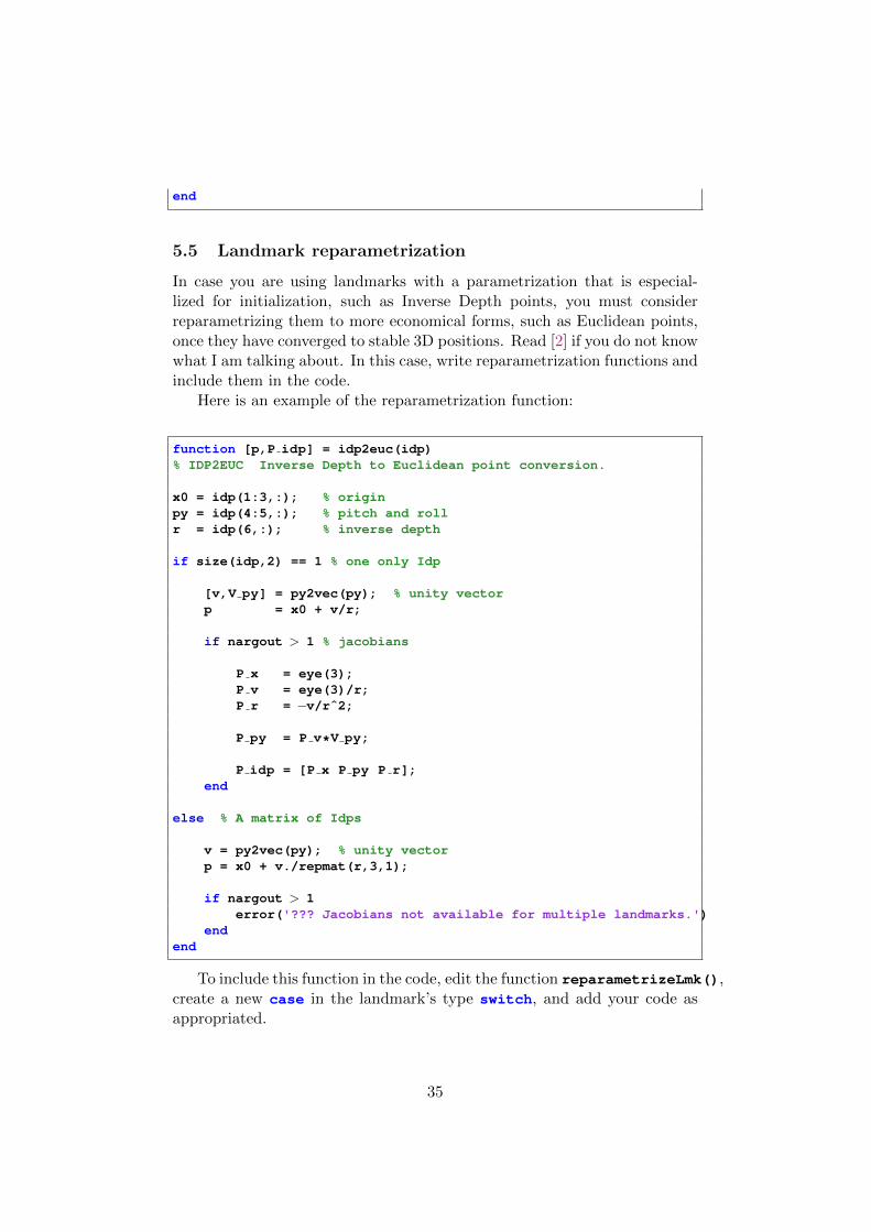
5.5 Landmark reparametrization

In case you are using landmarks with a parametrization that is especial-lized for initialization, such as Inverse Depth points, you must considerreparametrizing them to more economical forms, such as Euclidean points,once they have converged to stable 3D positions. Read [2] if you do not knowwhat I am talking about. In this case, write reparametrization functions andinclude them in the code.

Here is an example of the reparametrization function:

function [p,P idp] = idp2euc(idp)% IDP2EUC Inverse Depth to Euclidean point conversion.

x0 = idp(1:3,:); % originpy = idp(4:5,:); % pitch and rollr = idp(6,:); % inverse depth

if size(idp,2) == 1 % one only Idp

[v,V py] = py2vec(py); % unity vectorp = x0 + v/r;

if nargout > 1 % jacobians

P x = eye(3);P v = eye(3)/r;P r = −v/rˆ2;

P py = P v*V py;

P idp = [P x P py P r];end

else % A matrix of Idps

v = py2vec(py); % unity vectorp = x0 + v./repmat(r,3,1);

if nargout > 1error('??? Jacobians not available for multiple landmarks.')

endend

To include this function in the code, edit the function reparametrizeLmk(),create a new case in the landmark’s type switch, and add your code asappropriated.

35

Another example of reparametrization is hmg2euc(). It transforms ho-mogeneous points to the Euclidean space.

5.6 Landmark parameters out of the SLAM map

There may be some landmark parameters that are not part of the stochasticstate vector estimated by SLAM. The number and nature of these parame-ters depend on the landmark type and cannot be generalized.

The direct and inverse observation models must be complemented withthe appropriate methods to initialize and update these parameters. In thetoolbox, we use the functions initLmkParams and updateLmkParams.

Examples of such parameters are:

• The endpoints of segment landmarks. See [8, 17] for examples of set-ting and updating. Initialization and updating of segment endpointsfor lines of the type Plucker are supported in this toolbox. Checkfunctions retroProjPlkEndPnts and updatePlkLinEndPnts.

• The landmark’s appearance information, used in appearance-basedfeature matching. See [4, 15] for examples on setting and using theseparameters. See [9] for an example of updating them.

5.7 Graphics

Each new landmark needs its own drawing methods and, possibly, dedicatedgraphic data structures.

5.7.1 Graphic handles

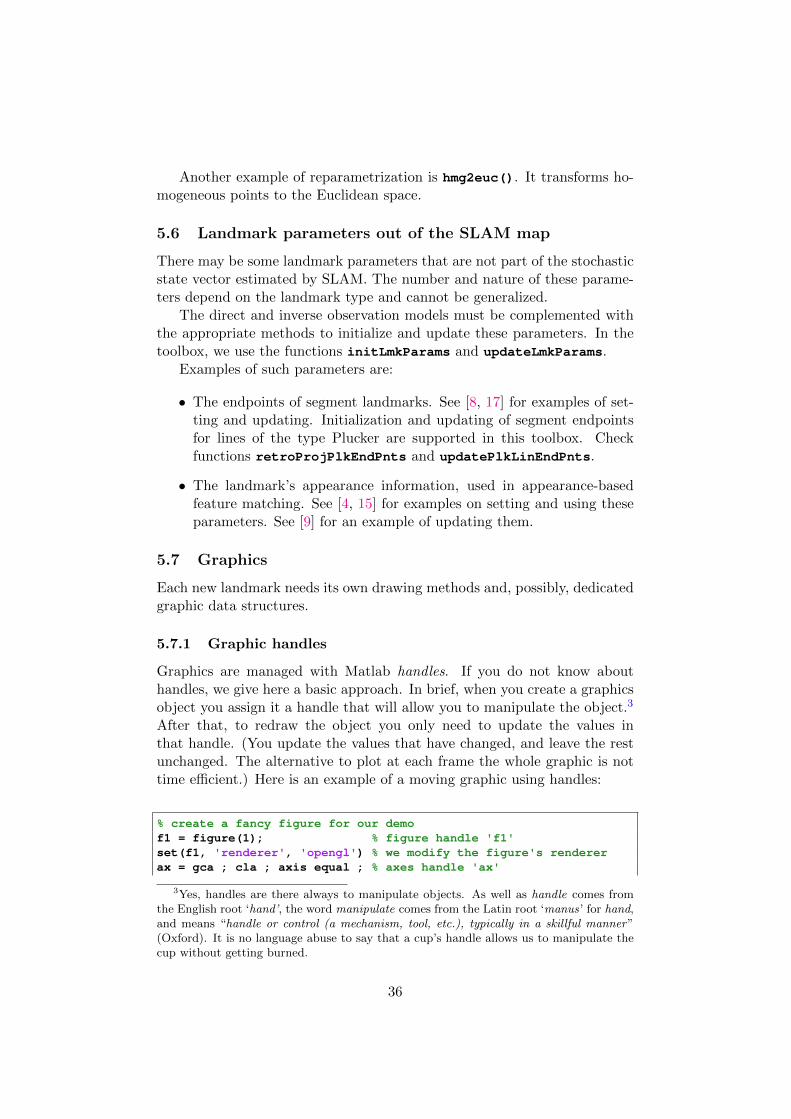
Graphics are managed with Matlab handles. If you do not know abouthandles, we give here a basic approach. In brief, when you create a graphicsobject you assign it a handle that will allow you to manipulate the object.3

After that, to redraw the object you only need to update the values inthat handle. (You update the values that have changed, and leave the restunchanged. The alternative to plot at each frame the whole graphic is nottime efficient.) Here is an example of a moving graphic using handles:

% create a fancy figure for our demof1 = figure(1); % figure handle 'f1'set(f1, 'renderer', 'opengl') % we modify the figure's rendererax = gca ; cla ; axis equal ; % axes handle 'ax'

3Yes, handles are there always to manipulate objects. As well as handle comes fromthe English root ‘hand’, the word manipulate comes from the Latin root ‘manus’ for hand,and means “handle or control (a mechanism, tool, etc.), typically in a skillful manner”(Oxford). It is no language abuse to say that a cup’s handle allows us to manipulate thecup without getting burned.

36

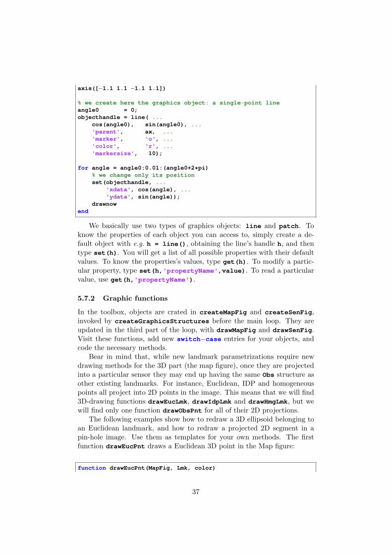
axis([−1.1 1.1 −1.1 1.1])

% we create here the graphics object: a single−point lineangle0 = 0;objecthandle = line( ...

cos(angle0), sin(angle0), ...'parent', ax, ...'marker', 'o', ...'color', 'r', ...'markersize', 10);

for angle = angle0:0.01:(angle0+2*pi)% we change only its positionset(objecthandle, ...

'xdata', cos(angle), ...'ydata', sin(angle));

drawnowend

We basically use two types of graphics objects: line and patch. Toknow the properties of each object you can access to, simply create a de-fault object with e.g. h = line(), obtaining the line’s handle h, and thentype set(h). You will get a list of all possible properties with their defaultvalues. To know the properties’s values, type get(h). To modify a partic-ular property, type set(h,'propertyName',value). To read a particularvalue, use get(h,'propertyName').

5.7.2 Graphic functions

In the toolbox, objects are crated in createMapFig and createSenFig,invoked by createGraphicsStructures before the main loop. They areupdated in the third part of the loop, with drawMapFig and drawSenFig.Visit these functions, add new switch−case entries for your objects, andcode the necessary methods.

Bear in mind that, while new landmark parametrizations require newdrawing methods for the 3D part (the map figure), once they are projectedinto a particular sensor they may end up having the same Obs structure asother existing landmarks. For instance, Euclidean, IDP and homogeneouspoints all project into 2D points in the image. This means that we will find3D-drawing functions drawEucLmk, drawIdpLmk and drawHmgLmk, but wewill find only one function drawObsPnt for all of their 2D projections.

The following examples show how to redraw a 3D ellipsoid belonging toan Euclidean landmark, and how to redraw a projected 2D segment in apin-hole image. Use them as templates for your own methods. The firstfunction drawEucPnt draws a Euclidean 3D point in the Map figure:

function drawEucPnt(MapFig, Lmk, color)

37

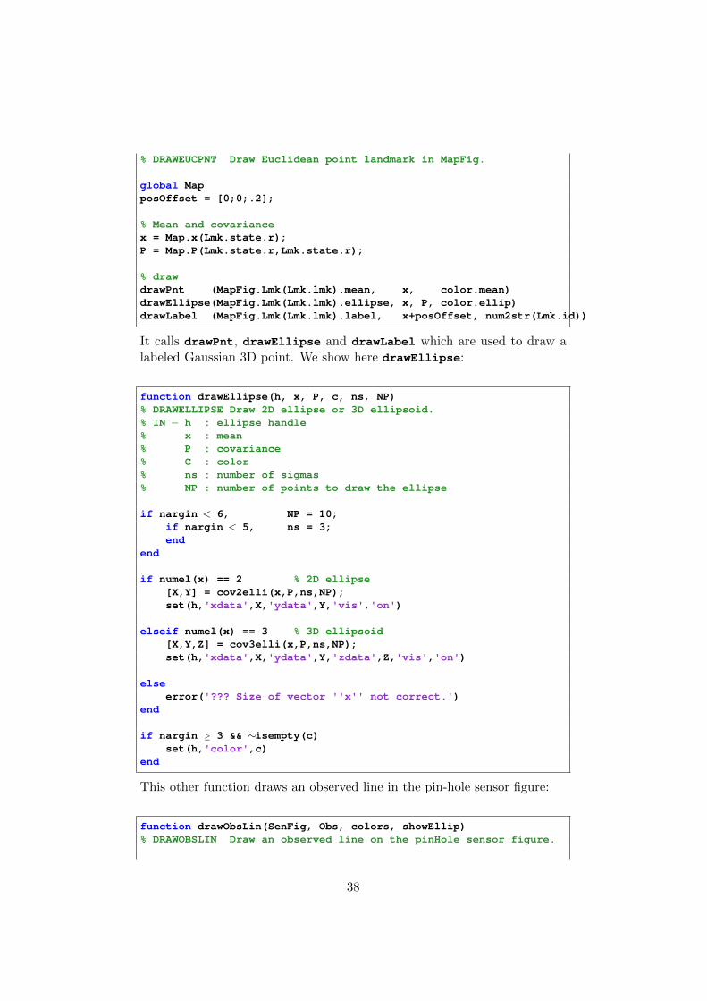
% DRAWEUCPNT Draw Euclidean point landmark in MapFig.

global MapposOffset = [0;0;.2];

% Mean and covariancex = Map.x(Lmk.state.r);P = Map.P(Lmk.state.r,Lmk.state.r);

% drawdrawPnt (MapFig.Lmk(Lmk.lmk).mean, x, color.mean)drawEllipse(MapFig.Lmk(Lmk.lmk).ellipse, x, P, color.ellip)drawLabel (MapFig.Lmk(Lmk.lmk).label, x+posOffset, num2str(Lmk.id))

It calls drawPnt, drawEllipse and drawLabel which are used to draw alabeled Gaussian 3D point. We show here drawEllipse:

function drawEllipse(h, x, P, c, ns, NP)% DRAWELLIPSE Draw 2D ellipse or 3D ellipsoid.% IN − h : ellipse handle% x : mean% P : covariance% C : color% ns : number of sigmas% NP : number of points to draw the ellipse

if nargin < 6, NP = 10;if nargin < 5, ns = 3;end

end

if numel(x) == 2 % 2D ellipse[X,Y] = cov2elli(x,P,ns,NP);set(h,'xdata',X,'ydata',Y,'vis','on')

elseif numel(x) == 3 % 3D ellipsoid[X,Y,Z] = cov3elli(x,P,ns,NP);set(h,'xdata',X,'ydata',Y,'zdata',Z,'vis','on')

elseerror('??? Size of vector ''x'' not correct.')

end

if nargin ≥ 3 && ∼isempty(c)set(h,'color',c)

end

This other function draws an observed line in the pin-hole sensor figure:

function drawObsLin(SenFig, Obs, colors, showEllip)% DRAWOBSLIN Draw an observed line on the pinHole sensor figure.

38

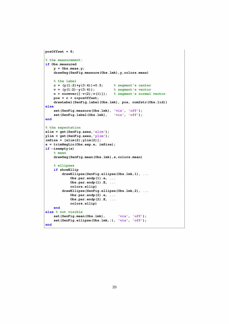
posOffset = 8;

% the measurement:if Obs.measured

y = Obs.meas.y;drawSeg(SenFig.measure(Obs.lmk),y,colors.meas)

% the labelc = (y(1:2)+y(3:4))*0.5; % segment's centerv = (y(1:2)−y(3:4)); % segment's vectorn = normvec([−v(2);v(1)]); % segment's normal vectorpos = c + n*posOffset;drawLabel(SenFig.label(Obs.lmk), pos, num2str(Obs.lid))

elseset(SenFig.measure(Obs.lmk), 'vis', 'off');set(SenFig.label(Obs.lmk), 'vis', 'off');

end

% the expectationxlim = get(SenFig.axes,'xlim');ylim = get(SenFig.axes,'ylim');imSize = [xlim(2);ylim(2)];s = trimHmgLin(Obs.exp.e, imSize);if ∼isempty(s)

% meandrawSeg(SenFig.mean(Obs.lmk),s,colors.mean)

% ellipsesif showEllip

drawEllipse(SenFig.ellipse(Obs.lmk,1), ...Obs.par.endp(1).e, ...Obs.par.endp(1).E, ...colors.ellip)

drawEllipse(SenFig.ellipse(Obs.lmk,2), ...Obs.par.endp(2).e, ...Obs.par.endp(2).E, ...colors.ellip)

endelse % not visible

set(SenFig.mean(Obs.lmk), 'vis', 'off');set(SenFig.ellipse(Obs.lmk,:), 'vis', 'off');

end

39

6 Extensions

You want to extend the capabilities of this toolbox. Here are some sugges-tions:

Combined points and lines: SLAM using both points and lines. Thisshould be relatively easy to implement, but at this time the toolboxdoes not support it. If you want to try, check and modify the featuredetection and landmark initialization sections (all in initNewLmks.m).Updates and rendering should work without problems.

Multi-map: Multi-map operation for consistent large-scale SLAM. Basi-cally, you should surround the main loop in slamtb.m with anotherloop managing the closing and creation of maps and performing themulti-map loop closures.

Other sensors: Use of sensors other than the pin-hole camera. This is amatter of building new observation models as explained in Section 5.

Real images: Use of real data, avoiding all the simulation part. Refer tothe following section for general guidelines.

6.1 Extension with real images

The toolbox does not support working with real images; you need to imple-ment it.

Basically, you should remove the whole SIMULATION section in slamtb.mand substitute it by a few lines of code loading an image into Raw(sen).data.img,setting Raw(sen).type to 'image'. Then, you need to code the fea-ture detection and matching functions for real images, inserting them ininitNewLmk.m and matchFeature.m respectively.

6.1.1 Loading, storing and displaying images

To load an image into the Raw structure, you can simply do:

Raw(sen).data.img = imread(imageFileName);

where imageFileName can be built at each frame with e.g.

imageFileName = sprintf('PATH/image%05d.png',currentFrame);

However, it might be more efficient to declare the image global, like:

global Img

40

% [...]Img{sen} = imread(imgFileName);

and ignore Raw(sen).data.img. This will speed up your algorithm. Iadvise you to use a cell array Img{sen} to be able to handle more than onecamera automatically, even if the images from each camera have differentsizes.

You may want to be sure that the image is grayscale, with just onechannel, and with just 8 bits depth. You can convert the image to anyformat you want using standard Matlab functions.

Regarding the graphics part, the toolbox already initializes a image han-dler in SenFig(sen).img, and updates it at each frame with the contentsof Raw(sen).data.img. To update it using a global image Img{sen}, editdrawSenFig.m and modify the appropriate code.

6.1.2 Some image processing tools

For what concerns the image processing, the toolbox has a few functions,located in directory DetectionMatching/, that might help you in doingthis without the need of the Matlab’s Image Processing toolbox:

harris strongest.m gives you the strongest Harris point in an image.You normally give it a fraction of the image where you know no land-marks are tracked, and ask the function to give you one point there.This is used for landmark detection just before initialization.

[point,sc] = harris strongest(im,sigma,mrg,edgerej)

pix2patch.m extracts a rectangular image patch centered on a pixel. Inorder to speed up some computations of the ZNCC, it is useful todefine the patch structure as follows: patch.I is the patch image (of9× 9 to 15× 15 pixels as detailed below). patch.SI is the sum of allpixels. And patch.SII is the sum of the squares of the pixels. Thisfunction does the job for you, and it already accepts working withglobal images Img.

ptch = pix2patch(I,pix,hsize,vsize)

zncc.m is the zero-mean normalized correlation coefficient, used for featurematching. It basically compares 2 patches and gives you a score ofsimilarity in the range [-1 1]. Other correlation scores are ssd.m andcensus.m.

41

sc = zncc(I,J,SI,SII,SJ,SJJ)

imresize2.m is used to modify the reference patch before correlation, sothat the appearance of the reference patch resembles at maximum thatof the feature to match in the current image. You use the estimatedrotation and distance variation to infer zoom and rotation parametersfor patch resizing. This function may need some improvements to workfully satisfactorily, but it is good enough for a start. If you have theImage processing toolbox, you can try imtransform.m instead.

out im = imresize2(im,H)

patchResize.m uses imresize2.m to create a modified version of thestructure patch.

rpatch = patchResize(opatch,r)

6.1.3 The active-search algorithm

The work of implementing SLAM with real images is long. I recommend youread the literature about ”active search” techniques [4, 6, 15]. The activesearch algorithm takes care of the following:

1. At initialization time (inside initNewLmk.m, and then in detectFeature.m)

(a) Define a grid in the image plane, for example 5x5 cells dividingthe image in equal subimages. I recommend you store this gridsomewhere in the Sen structure so that you have easy access toit. You create the grid at startup, in createSensors.m. Youalso need to define the user-configurable grid characteristics be-forehand in userData.m, in the Sensor{i} section.

(b) Project all mapped landmarks into the image. For each projectedlandmark (only the mean is needed), set the grid cell where themean has been projected to true or 'occupied'.4

(c) When done, randomly select one only cell which is not 'occupied'.Extract the image of that cell.

(d) Detect the best Harris point in this image cell, with harris strongest.m.Set the resulting pixel pix as the landmark measurement with

4You may want to relegate this peace of code to the correctKnownLmks.m func-tion, as in this function all landmarks are being projected already. This way you savecomputation time, but the resulting code is less compact. It’s up to you.

42

meas.y = pix and meas.R = pixnoiseˆ2*eye(2). The tool-box will use this measurement for landmark initialization. To en-sure a proper graphics rendering, set also the expectation exp.e = meas.yand exp.E = meas.R.

(e) Check if the detected point is good enough by putting a thresholdon the Harris score returned. This ”feature quality threshold”needs to be created beforehand. A good place to store it is inObs.init.featQualityTh, defined in userData.m.

(f) If successful, store a 9× 9 to 15× 15 pixels patch around the de-tected point, and the current camera position and orientation, inan ”appearance” variable app. This will become the landmark’sdescriptor or ”signature” for future matchings (on successful ini-tialization, the toolbox will store it for you in Lmk.sig).

(g) Create a unique identifier for the new landmark (a number).Name it newId. The toolbox will assign it to Lmk and Obs struc-tures for you.

(h) Proceed to initialization (this is already coded in initNewLmk.m).

basically, you enter code 1a—1g in the case 'image' in detectFeaturewithin initNewLmk.m.

function [Lmk,Obs] = initNewLmk(Rob, Sen, Raw, Lmk, Obs, Opt)

% [...]

% Feature detectionswitch Raw.type

case {'simu','dump'}[newId, app, meas, exp, inn] = simDetectFeat(...

Opt.init.initType, ...[Lmk([Lmk.used]).id], ...Raw.data, ...Sen.par.pixCov, ...Sen.par.imSize);

case 'image' % <−−− INSERT YOUR FUNCTION HERE% NYI : Not Yet Implemented. Create detectFeat.m and call:% [newId, app, meas, exp, inn] = detectFeat(...);error('??? Raw type ''%s'' not yet implemented.', Raw.type);

end

% [...]

2. At correction time (inside correctKnownLmks.m, and then inside matchFeature.m)

(a) Project all mapped landmarks (this is already done).

43

(b) Select the set of landmarks to observe (done).

(c) For each selected observation, proceed as follows.

(d) Define a rectangular search region based on the projection meanObs.exp.x and the 3-sigma ellipse Obs.inn.P. The mean is thecenter, and the square roots of the diagonals of the covariance arethe sigmas, σu and σv. You need to build a rectangle that goes±3σ at each side of the center.

(e) Using the current camera position and orientation, and the storedposition and orientation in Lmk.sig.pose0, compute a zoomingfactor and a rotation to be applied to the stored patch Lmk.sig.patchbefore scanning. Store this predicted appearance in Obs.app.pred.

(f) Scan the rectangular region for the modified patch, using zncc.mas the preferred ZNCC correlation score. Store the best matchpatch in Obs.app.curr, and the score in Obs.app.sc. Store thebest pixel as the measurement, in Obs.meas.y. Set Obs.measured = true.

(g) On completion, test if the ZNCC score is greater than a threshold(0.95 minimum). This ”appearance score threshold” needs to becreated beforehand. A good place to store it is in Obs.correct.appScTh,defined in userData.m. If successful, set Obs.matched = true.

(h) Test the Mahalanobis distance between the expectation and themeasurement to be smaller than a threshold. If passed, set Obs.inlier = true.This is already coded in correctKnownLmks.m.

(i) Proceed with landmark correction (already done).

basically, you need to code 2c—2g inside matchFeature.m. Useswitch / case statements to select which kind of processing youwill do depending on the Raw.type data being 'image', 'simu',etc.

function Obs = matchFeature(Sen,Raw,Obs)

% [...]

switch Raw.typecase {'simu','dump'}

% [...]

case 'image'error('??? Feature matching for Raw data type ''%s'' not implemented yet.', Raw.type)% TODO: the 'image' case <−−− INSERT YOUR CODE HERE

end

Within matchFeature.m, do not forget to set the flags .measured, .matchedin structure Obs: they are important for the correct development of

44

the algorithm, especially in the graphics section. The landmark eventcounters .nSearch, nMatch, nInlier in structure Lmk are alreadyupdated by the toolbox.

It is long but doable. Good luck!

45

7 Bibliography selection

The following publications list is of mandatory reading for anyone wishingto understand/use/contribute to this toolbox.

• One article by myself and colleagues demonstrating performances ofseveral landmark parametrizations for monocular EKF-SLAM: [16].

• Articles by myself and colleagues about monocular SLAM and theextensions to multi-camera: [14, 13, 15, 17].

• My thesis [12], but not in all its extension. Read Chapter 6, andparticularly section 6.5 on Active Search.

• Articles by Andrew J. Davison, the most important contributor tomonocular EKF-SLAM, and his colleagues at Oxford, London andCambridge: [4, 5, 6, 9, 7].

• Articles from the University of Zaragoza, mostly on EKF-SLAM. Land-mark initialization using inverse-depth parametrization, and multi-map SLAM for large environments: [10, 2, 3, 11].

If this list is too long for your available time or patience, try this reducedversion of just 3 titles:

1. Davison on monocular SLAM [4].

2. Sola on landmark parametrizations for points and lines [16].

3. Sola on multi-camera SLAM [15].

46

References

[1] Simone Ceriani, Daniele Marzorati, Matteo Matteucci, Davide Migliore,and Domenico Giorgio Sorrenti. On feature parameterization for ekf-based monocular slam. In IFAC WC, 2011.

[2] Javier Civera, Andrew J. Davison, and Jose Marıa Martınez Montiel.Inverse Depth to Depth Conversion for Monocular SLAM. In IEEE Int.Conf. on Robotics and Automation, pages 2778 –2783, April 2007.

[3] Javier Civera, Andrew J. Davison, and Jose Marıa Martınez Montiel.Inverse depth parametrization for monocular SLAM. IEEE Trans. onRobotics, 24(5), 2008.

[4] Andrew J. Davison. Real-time simultaneous localisation and mappingwith a single camera. In Int. Conf. on Computer Vision, volume 2,pages 1403–1410, Nice, October 2003.

[5] Andrew J. Davison. Active search for real-time vision. Int. Conf. onComputer Vision, 1:66–73, 2005.

[6] Andrew J. Davison, Ian D. Reid, Nicholas D. Molton, and OlivierStasse. MonoSLAM: Real-time single camera SLAM. Trans. on PatternAnalysis and Machine Intelligence, 29(6):1052–1067, June 2007.

[7] Ethan Eade and Tom Drummond. Scalable monocular SLAM. IEEEInt. Conf. on Computer Vision and Pattern Recognition, 1:469–476,2006.

[8] Thomas Lemaire and Simon Lacroix. Monocular-vision based SLAMusing line segments. In IEEE Int. Conf. on Robotics and Automation,pages 2791–2796, Rome, Italy, 2007.

[9] Nicholas Molton, Andrew J. Davison, and Ian Reid. Locally planarpatch features for real-time structure from motion. In British MachineVision Conference, 2004.

[10] Jose Marıa Martınez Montiel, Javier Civera, and Andrew J. Davi-son. Unified inverse depth parametrization for monocular SLAM. InRobotics: Science and Systems, Philadelphia, USA, August 2006.

[11] L. M. Paz, Pedro Pinies, Juan Domingo Tardos, and Jose Neira. Largescale 6DOF SLAM with stereo-in-hand. IEEE Trans. on Robotics,24(5), 2008.

[12] Joan Sola. Towards Visual Localization, Mapping and Moving ObjectsTracking by a Mobile Robot: a Geometric and Probabilistic Approach.PhD thesis, Institut National Polytechnique de Toulouse, 2007.

47

[13] Joan Sola, Andre Monin, and Michel Devy. BiCamSLAM: Two timesmono is more than stereo. In IEEE Int. Conf. on Robotics and Au-tomation, pages 4795–4800, Rome, Italy, April 2007. IEEE.

[14] Joan Sola, Andre Monin, Michel Devy, and Thomas Lemaire. Unde-layed initialization in bearing only SLAM. In IEEE/RSJ Int. Conf. onIntelligent Robots and Systems, pages 2499–2504, Edmonton, Canada,2005. IEEE.

[15] Joan Sola, Andre Monin, Michel Devy, and Teresa Vidal-Calleja. Fus-ing monocular information in multi-camera SLAM. IEEE Trans. onRobotics, 24(5):958–968, October 2008.

[16] Joan Sola, Teresa Vidal-Calleja, Javier Civera, and Jose Marıa MartınezMontiel. Impact of landmark parametrization on monocular EKF-SLAM with points and lines. Int. Journal of Computer Vision,97(3):339–368, September 2011. Available online at Springer’s:http://www.springerlink.com/content/5u5176nj521kl3h0/.

[17] Joan Sola, Teresa Vidal-Calleja, and Michel Devy. Undelayed initial-ization of line segments in monocular SLAM. In IEEE/RSJ Int. Conf.on Intelligent Robots and Systems, pages 1553–1558, Saint Louis, USA,October 2009. IEEE.

48