DESIGN AND IMPLEMENTATION OF A 6 DOF PARALLEL …

DESIGN AND IMPLEMENTATION OF A 6 DOF PARALLEL MANIPULATOR

WITH PASSIVE FORCE CONTROL

By

BO ZHANG

A DISSERTATION PRESENTED TO THE GRADUATE SCHOOL OF THE UNIVERSITY OF FLORIDA IN PARTIAL FULFILLMENT

OF THE REQUIREMENTS FOR THE DEGREE OF DOCTOR OF PHILOSOPHY

UNIVERSITY OF FLORIDA

2005

Copyright 2005

by

Bo Zhang

iii

ACKNOWLEDGMENTS

The author wishes to express his great gratitude to Dr. Carl D. Crane, III, his

dissertation advisor, for suggesting the topic of this work, providing continuous guidance,

support and encouragement throughout this research. Also the author would like to

acknowledge the efforts of his supervisory committee members: Dr. John C. Ziegert, Dr.

Gloria J. Wiens, Dr. A. Antonio Arroyo and Dr. Rodney G. Roberts, whose time and

expertise were greatly appreciated.

The author wishes to acknowledge the guidance from Dr. Joseph Duffy; he will be

greatly missed. The author would like to thank Dr. Carol Chesney, Shannon Ridgeway,

Dr. Michael Griffis, Dr. Bob Bicker and Jean-Francois Kamath for their great help. He

also would like to thank his fellow students in the Center for Intelligent Machines and

Robotics for sharing their knowledge.

This research was performed with funding from the Department of Energy through

the University Research Program in Robotics (URPR), grant number DE-FG04-

86NE37967.

Finally, the author gives special appreciation to his parents, for their love, patience

and support.

iv

TABLE OF CONTENTS page

ACKNOWLEDGMENTS ................................................................................................. iii

LIST OF TABLES............................................................................................................. vi

LIST OF FIGURES ......................................................................................................... viii

ABSTRACT....................................................................................................................... xi

CHAPTER

1 MOTIVATION AND INTRODUCTION....................................................................1

Motivation.....................................................................................................................1 Introduction...................................................................................................................4

2 BACKGROUND AND LITERATURE REVIEW ....................................................11

Kinematics Analysis ...................................................................................................11 Singularity Analysis....................................................................................................13 Statics and Compliance Analysis................................................................................14 Compliance and Stiffness Matrix ...............................................................................17

3 PARALLEL PLATFORM DESIGN..........................................................................20

Design Specification...................................................................................................20 Conceptual Design......................................................................................................22 Prototype Design ........................................................................................................28

4 SINGULARITY ANALYSIS.....................................................................................34

5 STIFFNESS ANALYSIS OF COMPLIANT DEVICE .............................................41

Simple Planar Case Stiffness Analysis .......................................................................41 Planar Displacement and Force Representation .........................................................46 Stiffness Mapping for a Planar System ......................................................................48 Stiffness Matrix for Spatial Compliant Structures......................................................51

v

6 FORWARD ANALYSIS FOR SPECIAL 6-6 PARALLEL PLATFORM ...............65

Forward Kinematic Analysis for a 3-3 Platform ........................................................65 Forward Kinematic Analysis for Special 6-6 In-Parallel Platform ............................70

7 RESULTS AND CONCLUSION...............................................................................78

Calibration Experiment for the Force Sensor .............................................................78 Individual Leg Calibration Experiment ......................................................................80 Parallel Platform Force/Wrench Testing Experiment.................................................85 Determination of Stiffness Matrix at a Loaded Position ............................................95 Future Research ........................................................................................................106

APPENDIX MECHANICAL DRAWINGS OF THE PARTS FOR PCCFC..............107

LIST OF REFERENCES.................................................................................................114

BIOGRAPHICAL SKETCH ...........................................................................................118

vi

LIST OF TABLES

Table page 3-1 Design objective specification .................................................................................21

6-1 Mappings of angles of spherical four bar mechanism..............................................69

6-2 Parameter substitutions ............................................................................................75

7-1 Load cell regression statistics...................................................................................80

7-2 Force-torque Sensor Resolution ...............................................................................85

7-3 Repeatability experiment, method 1 (Encoder Counts) ...........................................86

7-4 Repeatability experiment, method 2 (Encoder Counts) ...........................................87

7-5 Forward analysis ......................................................................................................88

7-6 Spring constants .......................................................................................................92

7-7 Numerical experiment 1- encoder counts and leg lengths .......................................93






7-13 Numerical experiment 1 - wrench............................................................................94





vii


7-19 Measured leg connector lengths at positions A through F (all units mm) .............100

7-20 Displacement of leg connectors from unloaded home position at positions A through F (all units are encoder counts).................................................................101

viii

LIST OF FIGURES

Figure page 1-1 Passive compliance device for contact force control .................................................3

1-2 Serial structure............................................................................................................4

1-3 In-parallel platform ....................................................................................................5

1-4 General parallel platform. ..........................................................................................9

1-5 3-3 parallel platform...................................................................................................9

2-1 Remote Center Compliance Coupling......................................................................17

3-1 Plan view of octahedral 3-3 parallel platform..........................................................23

3-2 Special 6-6 parallel platform. ...................................................................................26

3-3 3-D model for special 6-6 parallel mechanism ........................................................27

3-4 Plan view of special 6-6 platform ............................................................................29

3-5 Flow chart of the design process ..............................................................................30

3-6 Assembled model for special 6-6 parallel platform .................................................32

3-7 Photo of the assembled parallel platform.................................................................33

4-1 Planar singularity......................................................................................................35

4-2 Plan view of a special 6-6 parallel platform.............................................................36

4-3 Plan view of the special singularity configuration ...................................................37

4-4 Photo of the parallel platform in singularity ............................................................39

5-1 Planar in-parallel springs..........................................................................................42

5-2 Planar serially connected springs system .................................................................43

5-3 Planar 2 DOF spring.................................................................................................44

ix

5-4 Planar compliant system...........................................................................................49

5-5 Stiffness mapping for a planar compliant system ....................................................50

5-6 3-D Model for special 6-6 parallel mechanism........................................................55

5-7 Top view of the special 6-6 configuration ...............................................................55

6-1 3-D drawing of the 3-3 in-parallel platform.............................................................67

6-2 A general spherical four-bar mechanism .................................................................69

6-3 3-3 in-parallel mechanism with three spherical four-bar linkages ...........................70

6-4 Special 6-6 platform and equivalent 3-3 platform ...................................................72

6-5 Definition of angles β and γ .....................................................................................73

6-6 Planar triangle ..........................................................................................................74

7-1 Load cell calibration experiment..............................................................................79

7-2 Load cell calibration experiment - opposite direction..............................................79

7-3 Calibration plot for leg-1..........................................................................................81






7-9 Photo of the testing experiment for the parallel platform ........................................85

7-10 Coordinate systems of the parallel platform ............................................................90

7-11 Compliant Platform Model.......................................................................................96

A-1 Strip holder. ............................................................................................................108

A-2 Lower leg part. .......................................................................................................109

A-3 Upper leg part.........................................................................................................110

A-4 Leg..........................................................................................................................111

x

A-5 Top plate.................................................................................................................112

A-6 Base plate. ..............................................................................................................113

xi

Abstract of Dissertation Presented to the Graduate School of the University of Florida in Partial Fulfillment of the Requirements for the Degree of Doctor of Philosophy

DESIGN AND IMPLEMENTATION OF A 6 DOF PARALLEL MANIPULATOR WITH PASSIVE FORCE CONTROL

By

Bo Zhang

August 2005

Chair: Carl D. Crane III Major Department: Mechanical and Aerospace Engineering

Parallel mechanism has been studied for several decades. It has various advantages

such as high stiffness, high accuracy and high payload capacity compared to the

commonly used serial mechanism. This work presents the design, analysis, and control

strategy for a parallel compliance coupler for force control (PCCFC) based on a parallel

platform design. The device is installed on the distal end of an industrial manipulator to

regulate the contact wrench experienced when the manipulator comes into contact with

objects in its environment. The parallel mechanism is comprised of a top platform and a

base platform that are connected by six instrumented compliant leg connectors. The pose

of the top platform relative to the base as well as the external wrench applied to the top

platform is determined by measuring the displacements of the individual leg connectors.

The serial robot then moves the PCCFC in order to achieve the desired contact wrench at

the distal end.

xii

A mechanical system has been fabricated with an emphasis placed on minimizing

the system size and minimizing friction at the joints. Each leg has been calibrated

individually off-line to determine connector properties, i.e., spring constant and free

length.

The spatial compliance matrix of the PCCFC has been studied to better understand

the compliant property of the passive manipulator. The forward analysis for the special

6-6 parallel platform as well as the kinematic control is also studied. The outcome of this

research will advance the contact force/torque and pose regulation for in-contact

operations.

1

CHAPTER 1 MOTIVATION AND INTRODUCTION

Motivation

With the development of robotics and control technologies, many tasks can now be

done with higher efficiency than ever before. Robotic systems can perform extremely

high precision operations in automatic assembly lines as well as perform operations in

environments that are too dangerous for humans to work in directly. Simple operations

can be completed by position control alone and manipulators are capable of high

repeatability which makes these operations easy to control. More complex operations

require the robot to be controlled as it manipulates a work piece which comes into contact

with other objects in its environment.

The control of forces during in-contact operations is a more difficult problem than

that which occurs during non-contact operations. For example, during an in-contact

operation it is necessary to monitor the loads applied externally to the end effector to

ensure that the forces and torques applied to the object being manipulated and the objects

in the environment do not exceed allowable specified values. The manipulator should

provide the appropriate loads to the object to function properly without exceeding the

external load limits of the object. As an example, the manipulator may need to implant a

prism-shaped part into a corresponding hole of a precision instrument. During the

assembly operation, the part should be carefully fitted with minimal collision so as not to

damage the component or the instrument.

2

Industrial manipulators have been in use since the mid 1970’s. Traditional serial

industrial robots can be positioned and oriented very accurately and moved along a

desired trajectory. However, without some form of force control, any positional

misalignment of the manipulator could cause unexpected yielding interaction with other

parts if the manipulated end-effector is rigidly positioned.

To satisfy these kinds of requirements, one solution is to integrate a force control

scheme into the manipulator controller where measured forces are fed back in a closed-

loop approach. Load cells that are commercially available are capable of measuring a

spatial wrench. These devices, however, are quite stiff and the response of the

manipulator may not be fast enough to prevent high contact forces. The focus of this

dissertation is on the creation and analysis of a more compliant spatial device that can be

incorporated into the control loop of a manipulator in order to successfully accomplish

the in-contact force control task.

Compliance control must be integrated in the robotic control when the manipulator

is handling some fragile or dangerous objects with force regulation. A properly designed

compliance control system has following advantages [Hua98]:

1. Avoiding collision and damage of the object and the environment.

2. Regulating the loads and wrench applied on the manipulator to meet any special external load requirements.

3. Compensating for the inevitable positional inaccuracies that results form rigid position/trajectory control.

A simple example is shown in Figure 1-1. A serial pair of actuated prismatic joints

supports a wheel via a two-spring system. The actuated prismatic joints are controlled so

that the wheel could maintain a desired contact force with a rigid wall [Gri91A, Duf96].

3

Figure 1-1. Passive compliance device for contact force control

The objective of this simple application is to control the contact force between the

wheel and the rigid wall when the wheel is rolling along the surface. The serial pair of

actuated prismatic joints supports the body containing points B1 and B2. This body is

connected to the wheel by two compliant connectors ( 1B C and 2B C ). The actuator drives

the end effector body with pure motion in the i and j directions to sustain the desired

contact force between the wheel and the environment and to move the wheel along the

surface as specified. This can be accomplished given the compliant propriety of the two

connectors (spring constants and free lengths) and the geometrical values of the

4

mechanism (θ1 and θ2). The relationship between a change in the actuator positions

( 1dδ and 2dδ ) and the change in contact force can be analytically determined.

Introduction

Most industrial manipulators are serial in structure. The serial structure is an open-

ended structure consisting of several links connected one after another as shown in Figure

1-2. The human arm is a good example of a serial manipulator. The kinematic diagrams

of most industrial manipulators look similar to that of the G.E. P-60 and PUMA 560

industrial robots in that most consist of seven links (including ground) interconnected by

six rotational joints using a special geometry (such as having three consecutive joint axes

being parallel or intersecting). These structures are well constructed, highly developed,

and are widely used in the industrial applications. Serial manipulators do not have closed

kinematical loops and are actuated at each joint along the serial linkage.

Figure 1-2. Serial structure

Accordingly, each actuator can significantly contribute to the net force/torque that

is applied to the end effector link, either to accelerate this link to cause it to move or to

influence the contact force and torque if the motion is restricted by the environment.

Since motions are provided serially, the effects of control and actuation errors are

5

compounded. Further, with serially connected links, the stiffness of the whole structure

may be low and it may be very difficult to realize very fast and highly accurate motions

with high stiffness.

Compared to the serial manipulator, the parallel manipulator is a closed-loop

mechanism in which the end-effecter (mobile platform) is connected to the base by at

least two independent kinematic chains (see for example Figure 1-3). With the multiple

closed loops, it can improve the stiffness of the manipulator because all the leg

connectors sustain the payload in a distributive manner as long as the device is far from a

singular configuration. The problem of end-point positioning error is also reduced due to

no accumulation of errors.

Figure 1-3. In-parallel platform

Hence this type of manipulator enjoys the advantages of compact, high speed, high

accuracy, high loading capacity, and high stiffness, compared to serial manipulators.

Disadvantages, however, include a limited work space due to connector actuation limits

and interference.

6

Therefore, the in-parallel mechanism is perceived to be a good counterpart and

necessary complement to that of the serial manipulator. It is very useful to combine these

two types of structures to utilize both advantages and decrease the weaknesses. One of

these applications is force control of serial manipulators with an in-parallel manipulator,

whose leg connectors are compliant and instrumented, is mounted at the end of the serial

arm. This is the approach that will be taken here in this dissertation; i.e., a commercially

available serial industrial manipulator will be augmented by attaching a compliant in-

parallel platform to the end effector so that contact forces can be effectively controlled.

Compared to parallel manipulators, the direct forward position analysis of serial

manipulators is quite simple and straightforward and the reverse position analysis is very

complex and often requires the solution of multiple non-linear equations to obtain

multiple solution sets. For the parallel manipulator, the opposite is the case in that the

reverse position analysis is straightforward while the forward position analysis is

complicated. This kind of phenomenon is usually referred to as serial-parallel duality.

There are similar duality properties between serial robots and fully parallel manipulator

with regards to instantaneous kinematics and statics.

The first parallel spatial industrial robot is credited to Pollard’s five degree-of-

freedom parallel spray painting manipulator [Pol40] that had three branches. This

manipulator was never actually built. In late 1950’s, Dr. Eric Gough invented the first

well-known octahedral hexapod with six struts symmetrically forming an octahedron

called the universal tire-testing machine to respond to the problem of aero-landing loads

[Gou62]. Then in 1965, Stewart published his paper of designing a parallel-actuated

mechanisms as a six-DOF flight simulator, which is different from the octahedral

7

hexapod and widely referred to as the “Stewart platform” [Ste65]. Stewart’s paper

gained much attention and has had a great impact on the subsequent development of

parallel mechanisms. Since then, much work has been done in the field of parallel

geometry and kinematics such as geometric analysis [Lee00, Hun98, Tsa99], kinematics

and statics [Das98A], and parallel dynamics and controls [Gri91B]. Relative works will

be discussed in a more detailed manner in the literature review section.

In addition to theoretical studies, experimental works on prototypes of the Stewart

platform have also been conducted for studying its property and performance. The fine

positioning and orienting capability of the Stewart platform make it very suitable for use

in control applications as dexterous wrists and various constructions of Stewart platform

based wrists.

Because there are different nomenclatures and definitions used by different

researchers in the field of parallel mechanisms, it is quite necessary to define the

nomenclature [Mer00] used in current research. The following terms are defined:

1. Parallel mechanism: A closed-loop mechanism in which the end-effecter (mobile platform) is connected to the base by at least two independent kinematic chains. It is also called Parallel Platform or a Parallel Kinematic Mechanism (PKM).

2. In-parallel mechanism: A 6-DOF parallel mechanism with two rigid bodies connected through six identical leg connectors, such as for example six extensible legs each with spherical joints at both ends or with a spherical joint at one end and a universal joint at the other.

3. Base Platform: The immovable plate of the parallel platform. It is also called the fixed platform.

4. Top Platform: The moving body connected to the base platform via extensible legs. It is also called moving platform or mobile platform.

5. Legs: The independent kinematic chains in parallel connecting the top platform and the base platform. Also called a connector.

6. Joint: Kinematic connection between two rigid bodies providing relative motion.

8

7. PCCFC: Parallel Compliance Coupler for Force Control. A parallel mechanism whose leg connectors are compliant and instrumented.

8. Platform Configuration: The combined positions and orientations of all leg connectors and the top platform.

9. Direct Analysis: Given the kinematic properties of the legs, determine the position and orientation of the top platform. Also called the forward analysis.

10. Reverse Analysis: Given the position and orientation of the top platform, determine the kinematic properties of the leg actuators.

11. M-N PKM: A PKM with M joint connection points on the base platform and N joint connection points on the top platform.

12. DOF: An abbreviating for degree of freedom.

A generalized parallel platform is shown in Figure 1-4 [Rid04]. In this example the

base platform and top platform are connected by six extensible legs. The joints

connecting the legs to the top platform and base platform are spherical joints, which

would introduce an additional trivial rotation of legs about their axes. These additional

freedoms will not affect the overall system performance and could be eliminated by

replacing the spherical joint on one end of each connector with a universal joint.

The above parallel platform has six legs connecting the base platform with the top

platform and there are six separate joint points on the base platform and top platform

respectively. This geometric arrangement it is called a 6-6 PKM or “6-6 platform”

according to the above nomenclature. The six joint points on the base platform are not

necessarily located on one plane, but it is often the case that all joint points lie on a single

plane and are arranged in some symmetric pattern.

9

Figure 1-4. General parallel platform [Rid02].

Besides the general 6-6 parallel platform, there are some other configurations. One

common configuration of a parallel mechanism is the 3-3 parallel manipulator as shown

in Figure 1-5.

Figure 1-5. 3-3 parallel platform.

Base Platform

Top Platform

Leg connector

Joint

10

The 3-3 parallel platform also has six connector legs, but each leg shares one joint

point with another leg on the base platform and similarly on the top platform. The three

shared joint points form a triangle on both the planar top platform and the planar base

platform. A literature review of these types of devices will be presented in the following

chapter.

11

CHAPTER 2 BACKGROUND AND LITERATURE REVIEW

Although it was Dr. Eric Gough [Gou62] who invented the first variable-length-

strut octahedral hexapod in England in the 1950’s, his parallel mechanism, also called the

universal tire-testing machine, did not draw much public attention. Then in 1965,

Stewart presented his paper on the design of a flight simulator based upon a 6 DOF

parallel platform [Ste65]. This work had a great impact on subsequent developments in

the field of parallel mechanisms. Since then, many researchers have done much work on

parallel mechanisms and both theoretical analyses and practical applications have been

studied.

Kinematics Analysis

The forward kinematic analysis of parallel mechanisms was one of the central

research interests in this field in the 1980s and 1990s. While the reverse kinematics

analysis, which is to calculate connector properties based on the top platform position and

orientation information, is quite straightforward, the forward kinematic analysis is

comparatively difficult to solve. The problem is to determine the position and orientation

information of the top platform (mobile platform) based on the connector properties, i.e.,

typically the connector lengths. Usually the legs are composed of actuated prismatic

joints that are connected to the top platform and base platform by a spherical joint at one

end and either a spherical or universal joint at the other. The connector properties are

generally referred to as the connector length or leg length as this parameter is usually

measured as part of a closed-loop feedback scheme to control the prismatic actuator.

12

It has been observed [Das00]that the closed-form solution for the forward

kinematics problem could be simplified by regulating the connector joint locations. The

simplest case is the 3-3 platform, which is degenerated by grouping the connector joints

into three pairs for both the top platform and base platform; each pair of connectors

shares one joint point. Although it is difficult to design a physical octahedral structure

with the concentric double-spherical joints that would have sufficient loading capacity

and adequate workspace due to collisions of the leg connectors themselves, the forward

analysis is the simplest for this class [Hun98]. The forward analysis of this device was

first solved by Griffis and Duffy [Gri89] who showed how the position and orientation of

the top platform can be determined with respect to the base when given the lengths of the

six connectors as well as the geometry of the connection points on the top and base. This

solution is a closed-form solution and is based on the analysis of the input/output

relationship of a series of three spherical four bar mechanisms. The resulting solution

yielded a single eighth degree polynomial in the square of one variable which resulted in

a total of sixteen distinct solution poses for a given set of connector lengths. Eight

solutions were reflected about the plane formed by the base connector points. The

solution technique was extended to solve other special configurations such as the 4-4 and

4-5 platforms with extended methods [Lin90, Lin94]. Other methods [Inn93, Mer92]

used constraints to solve the problem. First, part of the structure is ignored so that the

locus curves of the connector joints could be determined according to the connector and

joint properties. Then the removed part together with the angular and distance constraints

is added back for further determinations of the solution for the forward kinematics

analysis.

13

Some theoretical analyses [Rag93, Wen94] found that there are as many as 40

solutions for the forward kinematic equations. Hunt and Primrose used a geometrical

method to determine the maximum number of the assembly [Hun93]. In 1996, Wampler

[Wam96], found that the maximum number of possible configurations for a general

Stewart platform is forty by using a continuation method.

Singularity Analysis

A singular configuration is some special configuration in which the parallel

mechanism gains some uncontrollable freedom. For parallel manipulators, there are

different types of singularity conditions based on the analysis of the Jacobian matrix that

is formed from the lines of action of the six leg connectors [Zha04].

Both Tsai [Tsa99] and Merlet [Mer00] point out in their books that there are 3

types of singularities based on the Jacobian matrix analysis: the inverse kinematic

singularities where the manipulator loses one or more degrees of freedom and can resist

external loads in some directions; the direct kinematic singularities where the top

platform gains additional degree(s) of freedom and the parallel platform cannot sustain

external loads in certain direction (or just uncontrollable); and the combined singularities

which could exhibit the features of both the direct kinematic singularities and reverse

kinematic singularities.

Other researchers [Dan95, Ma91] found an interesting phenomenon called

architecture singularities, which means that some parallel manipulators with particular

configurations exhibit continuous motion capabilities in a relatively large portion of the

whole workspace with all actuators fixed. This kind of singularity should be avoided in

the early stage of design.

14

One of the reasons to study singularities is to avoid or restrict any singularities

from occurring within the effective workspace. Dasgupta [Das98B] developed a method

to plan paths with good performance in the workspace of the manipulator for some

special cases although there is not solid evidence to prove that the method is applicable to

all begin-pose-to-end-pose path planning.

Statics and Compliance Analysis

The forward static analysis is very straightforward as the end effector (top

platform) force can be directly mapped from the connector forces, as described by

[Fic86]. Duffy [Duf96] performed “stiffness mapping” analyses when considering the

relationship between the twist (instantaneous motion of the top platform) in response to a

change in the externally applied wrench. The mapping matrix (compliance matrix) is

related to the stiffness properties of the connectors as well as the geometric dimension

values.

The static equilibrium equation for a parallel mechanism with six leg connectors

can be written as

ŵ = {f ; m} = {f1 ; m01} + {f2 ; m02} + … + {f6 ; m06} (2-1) where ŵ is the applied external wrench applied to the top platform which is comprised of

a force f applied through the origin point of the reference coordinate system and a

moment m (dyname interpretation). The terms fi and mi, i = 1..6, represent the pure force

that is applied along each of the leg connectors, i.e., fi represents the force applied along

connector i and m0i represents the moment of the force along connector i measured with

respect to the origin of the reference frame.

This equation may also be written as

ŵ = f{S ; S0} = f1{S1 ; S0L1} + f2{S2 ; S0L2} + … + f6{S6 ; S0L6} (2-2)

15

where f is the magnitude of the external wrench, {S; S0} are the coordinates of the screw

associated with the wrench, fi represents the magnitude of the force along connector i,

and {Si ; S0Li} are the Plücker line coordinates of the line along connector i [Cra01].

This equation can also be written in matrix format as

1

2

1 2 3 4 5 6 3

0 01 02 03 04 05 06 4

5

6

fff

ffff

⎡ ⎤⎢ ⎥⎢ ⎥⎢ ⎥⎡ ⎤ ⎡ ⎤

= ⎢ ⎥⎢ ⎥ ⎢ ⎥⎣ ⎦ ⎣ ⎦ ⎢ ⎥

⎢ ⎥⎢ ⎥⎢ ⎥⎣ ⎦

S S S S S S SS S S S S S S

(2-3)

where the 6×6 matrix formed by the Plücker coordinates of the lines along the six leg

connectors comprises the Jacobian matrix that relates the force magnitudes along each leg

to the externally applied wrench.

A derivative of the above equation will yield a relationship between the changes in

individual leg forces to the change in the externally applied wrench. Griffis [Gri91A]

extended this analysis to show how the change in the externally applied wrench could be

mapped to the instantaneous motion of the top platform.

According to the static force analysis presented above, it is straightforward to

design a compliant parallel platform to detect forces and torques. Knowledge of the

spring constant and free length of each connector and measurement of the current leg

lengths allows for the computation of the external wrench, once a forward position

analysis is completed to determine the current pose. The first sensor of this type was

developed by Gaillet [Gai83] based on the 3-3 parallel octahedral structure. Griffis and

Duffy [Gri91B] then introduced the kinestatic control theory to simultaneously control

force and displacement for a certain constrained manipulator based on the general spatial

16

stiffness of a compliant coupling. In their theoretical analysis of the compliant control

strategy, a model of a passive Stewart platform with compliant legs was utilized to

describe the spatial stiffness of the parallel platform based wrench sensor.

Compared to the open loop Remote Center Compliance Modules (RCC) that are

commercially available (see Figure 2-1), the Stewart-platform-based force-torque sensor

can provide additional information about external wrench to assist force/ position control.

Dwarakanath and Crane [Dwa00], and Nguyen and Antrazi [Ngu91] studied a Stewart

platform based force sensor, using a LVDT to measure the compliant deflection for

wrench detection. Some researchers [Das94, Svi95] also considered the optimality of the

condition number of the force transformation matrix for isotropy and stability problems.

It is important that any wrench sensing device be far from a singularity

configuration. Lee [Lee94] defined the problem of “closeness” to a singularity measure

by defining what is known as quality index (QI) for planer in-parallel devices. Lee et al.

[Lee98] extended the definition of quality index to spatial 3-3 in-parallel devices. The

quality index is the ratio of the determinant of the matrix formed by the Plücker line

coordinates of the six connector legs of the platform in some arbitrary position to the

maximum value of the determinant that is possible for the in-parallel mechanism. The

index ranges from 0 to 1 and the maximum value of 1 refers to the optimal configuration.

Lee [Lee00] provides a detailed quality index presentation on several typical in-parallel

structures.

17

Figure 2-1. Remote Center Compliance Coupling

Compliance and Stiffness Matrix

The theory of screws is a very powerful tool to investigate the compliance or

stiffness characteristic of a compliant device. Ball [Bal00] first introduced the theory and

used it to describe the general motion of a rigid body. He presented the idea of the

principal screw of a rigid body, where a wrench applied along a principal screw of inertia

generates a twist on the same screw. The principal screw can be found by solving the

spatial eigenvector problem. Dimentberg [Dim65] analyzed the static and dynamic

properties of a spring suspended system using screw theory.

Patterson and Lipkin [Pat90] studied the necessary and sufficient conditions for the

existence of compliant axes and showed a new classification of general compliance

matrix based on the numbers of the compliant axes produced.

18

Loncaric [Lon87] also did research on unloaded compliant systems for the spatial

stiffness matrix and normal form analysis by using Lie groups. Then Loncaric [Lon91A]

used a geometric approach to define and analyze the elastic systems of rigid bodies and

described how to choose coordinates to simplify the interpretation of the compliance and

stiffness matrix.

Lipkin and Duffy [Lip88] presented a hybrid control theory for twist and wrench

control of a rigid body, and showed that it is based on the metric of elliptic geometry and

is noninvariant with the change of Euclidean unit length and change of basis.

Duffy [Duf96] analyzed planer parallel spring systems theoretically. Griffis and

Duffy [Gri91B] studied the non-symmetric stiffness behavior for a special octahedron

parallel platform with 6 springs as the connectors, and the stiffness mapping could be

represented by a 6×6 matrix [K]. Patterson and Lipkin [Pat92] also found that a

coordinate transformation changes the stiffness matrix into an asymmetric matrix but the

eigenvectors and eigenvalues are invariant under the coordinate transformation, and the

eigenvalue problems for compliance matrix and stiffness matrix are shown to be

equivalent.

Lipkin [Lip92A] introduce a geometric decomposition to diagonalize the 6×6

compliance matrix and the diagonal elements are the linear and rotational compliance and

stiffness values. It is also proved that the decomposition always exists for all cases.

Another paper [Lip92B] presents several geometric results of the 6×6 compliance matrix

via screw theory.

Huang and Schimmels [Hua00] also studied the decomposition of the stiffness

matrix by evaluating the rank-1 matrices that compose a spatial stiffness matrix by using

19

the stiffness-coupling index. The decomposition, which is also called eigenscrew

decomposition, is shown to be invariant in coordinate transformation with the concept of

screw springs.

Roberts [Rob02] points out that the normal stiffness matrix with a preload wrench

is asymmetric. However when only a small twist from the equilibrium pose is

considered, the spatial stiffness matrix is a symmetric positive semi-defined matrix and

the normal form could be derived from it.

Ciblak and Lipkin [Cib94] have shown that for a preload system with relative large

deflection from its original position, the stiffness matrix is no longer symmetric. In a

more recent study, Ciblak and Lipkin [Cib99] present a systematic approach to the

synthesis of Cartesian stiffness by springs using screw theory, and shown that a stiffness

matrix with rank n can be synthesized by at least n springs. Researchers [Cho02, Hua98,

Lon91B, Rob00] also work on synthesis for a predefined spatial stiffness matrix.

20

CHAPTER 3 PARALLEL PLATFORM DESIGN

The parallel mechanism offers a straightforward method to determine the external

wrench applied to the top platform based on measured leg lengths and knowledge of the

system geometry (location of joint points in top and base platforms), connector spring

constants, and connector spring free lengths. Because of this, the Passive Compliant

Coupler for Force Control (PCCFC) can be utilized in force feedback applications for

serial robots by employing it as a wrist element that is between the distal end of the

manipulator and the environment. In this chapter, a prototype for the compliant parallel

platform has been designed and tested in order to study the position/wrench control with

the PKM device.

Design Specification

The design process could roughly be composed by 3 stages [Tsa99]:

1. Product specification and planning stage, 2. Conceptual design stage, 3. Physical design stage.

During the first stage, the functionality, dimension, and other requirements are

specified for the development of the product. In the second stage, several rough

conceptual design alternatives are developed based on the product specification and the

one with best overall performance is chosen to be developed. In the last stage the

dimensional and functional design, analysis and optimization, assembly simulation,

material selection, and engineering documentation are completed. Although the third

21

stage usually is the most time-consuming stage, the first two stages have great impact on

design results and cost control.

In the PCCFC specification and planning stage, the product’s geometrical and

functional requirements are specified as follows:

SP1: The mechanism should be compliant in nature to measure contact loads;

SP2: The mechanism should have 6 degrees of freedom;

SP3: The mechanism should be a spatial parallel structure;

SP4: The mechanism should be ability to measure loads without large errors;

SP5: the structure should have a relatively compact size.

As mentioned in the previous chapter, the Stewart platform is a promising structure

for such spatial compliant devices. The Stewart platform structure satisfies the SP2 and

SP3 criteria. With each connector being composed of a prismatic joint and compliant

component, the SP1 and SP4 criteria could also be satisfied. One of the main advantages

of the Stewart platform is that it can withstand a large payload (compared to serial

geometries) with relative compact size. As a result, the dimensional requirement - SP5

could be met during the conceptual design and physical design stage. The detailed design

specifications are presented in Table 3-1. Note that in this table, the direction of the z

axis that is referred to is perpendicular to the plane of the base platform.

Table 3-1. Design objective specification Specification Range

Individual Connector Deflection : Magnitude ±5mm

Maximum perpendicular load: Magnitude 50N

Motion range in Z direction: Magnitude ±4mm

Motion range in X,Y direction: Magnitude ±3.5mm

22

Table 3-1. Continued Specification Range

Rotation range about Z axis: Magnitude ±6°

Rotation range about X,Y axis: Magnitude ±4°

Position Measuring Resolution: 0.01mm

Conceptual Design

In the conceptual design stage, a “best” conceptual design is selected from among

alternatives. The 3-3 octahedral structure was the first to be considered since it is the

simplest structure of its kind.

The mobility of general spatial mechanisms can be calculated from the Grübler

Criterion [Tsa99]:

∑=

−λ−−λ=j

1ii )f()1n(M , (3-1)

where:

M: Mobility, or number of degree of freedom of the system.

λ : Degrees of freedom of the space in which a mechanism is intended to function, for the

spatial case, λ = 6

n : Number of links in the mechanism, including the fixed link

j : Numbers of joints in a mechanism, assuming that all the joints are binary.

if : Degrees of relative motion permitted by joint i .

The octahedral 3-3 parallel platform is shown in Figure 3-1. It is the simplest

geometry for a spatial parallel platform. For the 3-3 parallel platform, the octahedron has

a top platform and a base platform, 6 connectors, and 6 concentric spherical joints, three

on the base platform and three on the top platform. Each connector is treated as 2 bodies

23

connected by a prismatic joint. Thus there are a total of 14 bodies; 2 for each of the 6

legs, the top platform, and the base platform. Each spherical joint has 3 relative degrees

of freedom and thus there are a total of 12 joints that each has 3 degrees of relative

freedom.

Figure 3-1. Plan view of octahedral 3-3 parallel platform

For this case, the mobility equation becomes

12303678)16()36()114(6M6

1i

12

1i=−−=−−−−−= ∑∑

==

(3-2)

Six out of the 12 degrees of freedom are trivial in that each leg connector can rotate

about its own axis. Eliminating these from consideration results in a 6 degree of freedom

device.

The forward kinematic analysis was first performed by Griffis and Duffy [Gri89].

They discovered that a maximum of sixteen pose configurations can exist for this device

(eight above the base platform and eight more reflections below the base platform) when

given a set of leg connector lengths. Hunt does a comprehensive study of the octahedral

24

3-3 parallel platform [Hun98]. Lee [Lee94] analyzed the singular configurations of this

device and defined the problem of “closeness” to a singularity by defining what is known

as the quality index (QI) for planer in-parallel devices. Lee et al. [Lee98] extended the

definition of quality index to the spatial 3-3 in-parallel device. The quality index is the

ratio of the determinant of the matrix formed by the Plücker line coordinates of the six

connector legs of the platform in some arbitrary position to the maximum value of

determinant that is possible for the in-parallel mechanism. This index is a dimensionless

value:

max||||

JJ

=λ , (3-3)

where J is the matrix of the line coordinates. The quality index has a maximum value of

1 at an optimal configuration that is shown to correspond to the maximum value of the

determinant. As the top platform departs from this configuration relative to the base, the

determinant would decrease, and at some positions and orientations it can reach zero

which indicates an uncontrollable singularity state.

As previously stated, the mechanism has been designed such that the determinant

of the matrix J will be near the maximum at the unloaded home position. Lee [Lee00]

showed that for a 3-3 platform with a top triangle of side length a and a bottom triangle of

side length b, that the maximum value of the determinant of J would occur when the top

platform was parallel to the base and was rotated as depicted by the plan view shown in

Figure 3-1. The determinant of the matrix J was shown to be given by

32

22

333

h3

baba4

hba33

⎭⎬⎫

⎩⎨⎧

++−

=J (3-4)

25

where h is the separation distance or height of the top platform with respect to the base.

Lee proved that the maximum value for the determinant of J would occur when

2 21 ( )

3h a ab b= − + . (3-5)

and 2b a= . (3-6)

From (3-5) and (3-6), it is easy to obtain

2 2b a h= = . (3-7)

Although the geometric configuration of the 3-3 parallel platform has the simplest

geometry with regards to the forward analysis, it is difficult to design and implement in

practice due to the pair of concentric spherical joints or other type of universal joints that

connect each leg to the base and top platform. These kind of concentric joint pairs are

not only very difficult to manufacture but also very hard to have sufficient payload

capacity. This configuration also induces unwanted interference between moving legs.

One other alternative is the 6-3 platform, which has six points of connection on the

base platform and three points of connection on the top platform. While this 6-3

configuration has less concentric joints pair in the base platform, it still has the same

difficulty and complicated arrangement of joint connections on the top platform. In order

to completely eliminate the need for coincident connections, the 6-6 parallel platform was

studied. The forward analysis for a general 6-6 platform, however, is very complicated

requiring lengthy computation and resulting in a maximum of forty configurations.

Griffis and Duffy [Gri93] developed a special 6-6 platform geometry, however,

where the forward analysis was comparable in difficulty to that of the 3-3 platform. As

26

opposed to a general 6-6 parallel platform, the special 6-6 platform has six leg connector

points in a plane on the top and base platforms. The arrangement of these connecting

points is such that three connecting points of the platform define a triangle as the apices

and the other three connecting points lie on the sides of this triangle.

There are a few configurations of the leg connection: one configuration, known as

the “apex to apex”, has three of the legs attaching to the corners or apices of the triangle

of the top platform and the base platform, and the remaining legs are attached to the sides

or edges of the platform. The other preferred configuration is known as “apex to

midline” as shown in Figure 3-2.

Figure 3-2. Special 6-6 parallel platform.

27

In order to eliminate the six additional rotational freedoms, the six spherical joints

connecting the top platform and leg connectors are replaced by universal joints. Equation

(3-1) is utilized here to calculate the mobility of the special 6-6 parallel platform

630241878)16()26()36()114(6M6

1i

6

1i

6

1i=−−−=−−−−−−−= ∑∑∑

===

(3-8)

The legs 1-6 are arranged in such a way that each of them is connecting to a corner

connecting point on either the top or base platform while the other connecting point is in

the midline of the triangle of the opposing platform. For example, leg 6 is connecting the

top platform 19 on the corner connecting point 18 with the base platform 20 on the

midline connecting point 12. Griffis noted that this particular configuration is singular

Figure 3-3. 3-D model for special 6-6 parallel mechanism

If the midline connecting points are not exactly on the middle of the triangle side

and for each side of the triangle, and the points are distributed symmetrically, there are

two different configurations which are usually called “clockwise” configuration and

28

“anti-clockwise” (the rotation direction of the top platform when pressed) configuration

based on the plan view of the structure. There is no significant analytical difference

between the two configurations for the kinematic analysis and control, so only one

configuration is used to build the prototype. One computer generated model of these

configurations is shown in Figure 3-3.

Prototype Design

After choosing the desired configuration of the prototype, more detailed and

specific information about the parallel platform should be studied in order to build the

physical mechanism. One plan view of the configuration of the parallel platform is

shown in Figure 3-4.

The dimensional relationship between the top/base platform and the free length of

the legs was studied by Lee [Lee00] based on the optimal dimensional restriction for the

special 6-6 parallel platform stated in the previous section. The free lengths of the

connectors are calculated by the following equations:

(3-9)

As shown in Figure 3-4:

l: free length of the legs, divided into two groups based on the fact that there are two

different values for free length of the legs.

a: refers to the functional triangle edge length of the top form

b: refers to the functional triangle edge length of the base form.

θ: refers to the rotation angle of the top platform about the z-axis.

( )

( )

2 2 2 2

2 2 2 2

1 3 (3 3 1) (cos 3(2 1)sin )31 3 (cos 3(2 1) sin ) (3 3 1)3

long

short

l h a ab b

l h a ab b

ρ ρ θ ρ θ

θ ρ θ ρ ρ

= + − + − + − +

= + − − − + − +

29

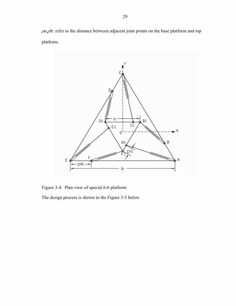
ρa,ρb: refer to the distance between adjacent joint points on the base platform and top

platform.

Figure 3-4. Plan view of special 6-6 platform

The design process is shown in the Figure 3-5 below

30

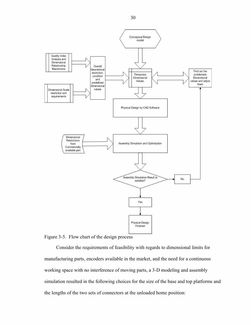
Figure 3-5. Flow chart of the design process

Consider the requirements of feasibility with regards to dimensional limits for

manufacturing parts, encoders available in the market, and the need for a continuous

working space with no interference of moving parts, a 3-D modeling and assembly

simulation resulted in the following choices for the size of the base and top platforms and

the lengths of the two sets of connectors at the unloaded home position:

31

a = 60 mm,

b =120 mm,

ρ = 28/120 = 0.2333,

h = a= 60mm,

Lshort = 68.021 mm,

Llong = 80.969 mm.

The elastic component is a crucial element for the passive compliant parallel

manipulator prototype. Precision linear springs were selected for use as the elastic

component to provide elongation and compression of the leg connectors. After carefully

studying and comparing different springs, a group of cylindrical precision springs with

different spring constants and the same high linear coefficient ( ± 5%) were selected to

use as the elastic component in the legs. The spring rates were respectively 8.755 N/mm,

2.627 N/mm and 0.8755 N/mm (or 50 lb/in, 15lb/in, and 5 lb/in). By using different

groups of springs, the stiffness matrix of the parallel platform could be changed by

replacing the spring and thus the device can be applied to different applications where the

expected force ranges are different.

The free length variation of each connector is measured by a linear optical encoder.

Each leg connector is comprised of two parts that translate with respect to each other and

are interconnected by the spring. The encoder read head is attached to one of the leg

parts and the encoder linear scale is attached to the other. The two leg parts are

constrained by a ball spline to ensure that they translate relative to one another and to

help maintain alignment of the encoder read head and linear scale.

32

The initial free length of each connector is measured by micro-photography with a

specially designed clamp apparatus. Since the six connecting points on the base platform

are in the same plane, the centers of the pseudo-spherical joints are also in the same

virtual plane. The free length of the connectors is defined as the distance between the

two centers of the joints, which connect the connector with the top platform and the base

platform.

Figure 3-6 shows renderings of the prototype device. Figure 3-7 presents a

photograph of the prototype.

A B Figure 3-6. Assembled model for special 6-6 parallel platform. A) Solid model, B)

Frame model.

33

Figure 3-7. Photo of the assembled parallel platform

34

CHAPTER 4 SINGULARITY ANALYSIS

In this chapter, a singularity analysis is presented and a special singularity

configuration for a special 6-6 parallel platform is analyzed.

It is important singularity configurations, which are identified as the case when

the Plücker line coordinates of the six leg connectors become linearly dependent, be

avoided throughout the effective workspace of the device. Singularities can occur in both

planar and spatial mechanisms. As an example, a planar structure is shown in Figure 4-1.

The structure is in a singular configuration when point S is at location (0, 0). At this

instant, considering the displacement of point S as the input and the displacement of point

D as the output, it is not possible to obtain a user desired velocity for point D, no matter

what the velocity of the input is. This condition where point S is at (0, 0) is called a

singular point as distinct from other simple points, which are also called regular points

[Hun78]. For this group of mechanism, a singularity only occurs when the mechanism

comes to some discrete special configuration while for all other points or configurations

the mechanism is normal or controllable. Particularly for parallel structures, it could be

said that singularity configurations exist in the workspace at those configurations where

the parallel structure gains some uncontrollable freedom.

35

Figure 4-1. Planar singularity

For spatial parallel manipulators, there are different types of singularity conditions

based on the analysis of the Jacobian matrix that is formed from the lines of action of the

six leg connectors. For example, a parallel manipulator may be able to resist external

loads in some directions with zero actuator forces at an inverse kinematical singular

configuration. Some manipulators can also have a different kind of singularity condition,

in which with all the actuators are locked, the top platform could still move

infinitesimally in some direction. Further, there are combined singularities that occur for

some special kinematic architecture when both conditions mentioned above occur

[Tsa99].

All the singularity conditions described above are temporary and conditional. This

means that only when the special geometrical configuration occurs, the mechanism will

function differently from the norm. The special 6-6 parallel platform is considered here

and the joint arrangement is shown in Figure 4-2.

Lee [Lee00] showed that when the dimensional ratio p=q=1/2, where p and q

represent the offset percentage of the joints in the base and top platform respectively, the

determinant of the Jacobian matrix is zero and the platform is in a singularity. He also

D

S

(0, 0)

36

identified the singularity case that occurs when the top platform rotates 90° around the Z-

axis.

Figure 4-2. Plan view of a special 6-6 parallel platform

Certain geometries exist, however, that are always singular. One planar example is

the parallelogram. A parallelogram with four revolute joints is normally unstable i.e., it

could not sustain external loads with internal angles unchanged. Compared to the very

stable triangle, such special geometries are often referred to as unstable as opposed to

being described as being in a singular state [Tsa 99].

Examples of unstable spatial mechanisms can also be found. Figure 4-3 shows the

particular case that was identified in this research. This special geometry is always

unstable, or in a singularity condition. It will be shown that the top platform will have

continuous mobility when the lengths of the six leg connectors are fixed. For this

pb qa

37

mechanism, both the top and the base platforms are equilateral triangles. The following

notation is used for this special singularity configuration:

a: the length of the side of the top equilateral triangle,

b: the length of the side of the base equilateral triangle,

q,p: a dimensionless number in the range of 0 to 0.5 that defines the offset distance of the

connection points (for example, the distance between points Ec1 and Ec2 is pb and the

distance between points B1 and B2 is qa),

h: the vertical distance from the geometric center of the base plate to the center of top

plate.

Figure 4-3. Plan view of the special singularity configuration

In order to simplify the process, here the structure will be analyzed only in an

initial configuration where the two plates are parallel and the relative rotation angle is

zero. The analysis process is the same for other positions and orientations. The matrix of

the line coordinates along the connectors for this configuration is written as

qa

38

( 1) (2 1) (1 2 ) (1 )2 2 2 2 2 2

3[ (3 1) ] 3( ) 3( ) 3[ (3 1) ] 3[ (2 3 ) 2 ] 3[2 (2 3 ) ]6 6 6 6 6 6

3 3 3 3(3 1) 2 3 3(2 3 )6 6 6 6 6 6

(2 1) (1 ) 02 2 2 2 23 36

q a b a p b q a b a p b qa pb

a q b b a b a a p b a q b a p b

h h h h h h

bh bh bh p bh bh p bh

bh p bh bh p bh pbh

qab p

− + − − − − − − −

− + − − − − − − − − −

− − − − −

− − − − −

− − 3 3 3 36 6 6 6 6

ab qab pab qab pab

⎡ ⎤⎢ ⎥⎢ ⎥⎢ ⎥⎢ ⎥⎢ ⎥⎢ ⎥⎢ ⎥⎢ ⎥⎢ ⎥⎢ ⎥⎢ ⎥⎢ ⎥⎢ ⎥− − −⎢ ⎥⎣ ⎦

(4-1)

The determinant of the Jacobian matrix is

,(4-2)

It was shown by Lee [Lee00] when analyzing the mechanism depicted in Figure 4-

2 that when p=q=0.5, the determinant of the Jacobian matrix equals zero and the structure

is unstable. For all other values for p and q in the range of 0 to 0.5, the structure is stable.

For the structure shown in Figure 4-3, the result is quite different. Clearly the

determinant of J is zero when p=q. Under the constraints 0≤q, p≤0.5, the term

2( ) 3 (1 )(1 )p q pq p q⎡ ⎤− + − −⎣ ⎦ is clearly nonnegative and is zero precisely when p=q=0.

Consequently, we have that under the natural physical constraints 0<q, p<0.5, the

determinant of J is zero if and only if p=q, regardless of the values for a, b, and h. This

means that the matrix is degenerate and the structure is singular and has gained some

uncontrollable freedom. Since the structure now could not sustain any external load, the

gravity of the top plate would change the configuration of the structure and would move

it downwards in Z direction with a counterclockwise rotation along the Z axis.

3 3 3 2 3 3 2 3 3

3 2

3( ) ( ) (9 9 3 9 9 3 )8

3 3 ( ) ( ) ( ) 3 (1 )(1 )8

Det J abh q p q p q qp q p p

abh p q p q pq p q

= − − − + +

⎡ ⎤= − − + − −⎣ ⎦

39

A photo of the platform model is shown in Figure 4-4. From the picture it can be

seen that the structure has collapsed due to the gravity effect until leg interference occurs.

The structure could sustain the gravity of the top plate in the shown state only because of

collisions of adjacent leg connectors which stops it from moving downwards further. The

top plate could easily be moved upwards with little upwards force applied.

Figure 4-4. Photo of the parallel platform in singularity

Although singular conditions are typically something to be avoided, there is one

application where this particular geometry would be of use. Platforms that incorporate

tensegrity must be in a state that when no external load is applied to the top platform, the

lines of action of the six leg connectors must be linearly dependent. Tensegrity based

platforms incorporate compliance such as springs to pre-stress certain leg connectors in

tension which will place the other connectors in compression. The internal forces in the

40

leg connectors can only sum to zero when the lines of action are linearly dependent.

Thus, the platform geometry discussed here could have particular application when

tensegrity is incorporated in the platform.

41

CHAPTER 5 STIFFNESS ANALYSIS OF COMPLIANT DEVICE

For a compliant component, such as a spring, the basic property of it is its stiffness.

Theoretically, no object is infinitely stiff; the only difference between a so called “stiff

component” and “compliant device” is that comparing with the “compliant” component,

the “stiff” component has a relatively much higher rigidity or stiffness. The spring is the

most commonly used compliant component. The stiffness property of a spring is usually

quantified by a ratio called the spring constant, also known as the elastic coefficient or

stiffness coefficient and is used to describe compliant devices.

In this chapter, simple analyses for planar compliant devices are introduced

together with an example of a compliant 2-D contact force control system. Then the

stiffness analysis of a 3-D system is studied using Screw theory. The stiffness matrix for

the special 6-6 parallel manipulator is developed and a numerical example is provided for

the specific design.

Simple Planar Case Stiffness Analysis

Hooke’s Law describes the fundamental relationship between an external force and

the compliant displacement in static equilibrium

0( )sF k l k l l= − ∆ = − − (5-1)

where sF is the force exerted on the spring (or more generally, the compliant component),

k is the spring constant, l is the current length of the spring, l0 is the free length, and l∆ is

the displacement from the equilibrium position.

42

Consider two springs that are connected in-parallel, with spring constants 1k and 2k

respectively. An external force is applied on the right end of the two springs and the

force direction is along the axes of the springs.

Figure 5-1. Planar in-parallel springs

The force in each spring can be calculated as

fs1 = -k1 ∆l1

fs2 = -k2 ∆l2

where in this case ∆l1 = ∆l2 = ∆l . The total force applied to the across the two springs

can be written as

fs = f1 + f2 (5-2)

The equivalent mapping of stiffness of the model is derived by:

1 1 2 2 1 2( ) ( )s

e

f k l k l k k lk l

= − ∆ + ∆ = − + ∆= − ∆

, (5-3)

where ek is the equivalent stiffness/spring constant of the in-parallel connected springs. It

is the sum of the individual spring constants. This shows that when compliant

components are connected in-parallel, the overall equivalent stiffness is much higher than

the stiffness of any individual compliant component.

sf

1sf

2sf

1k

2k

43

Figure 5-2. Planar serially connected springs system

Now consider two springs connected in series, as shown in Figure 5-2 above. The

axes of the two springs are collinear and they are connected end to end. The direction of

the external force applied on them is also along the axes of the springs. The derivation is

quite simple, so only the result is provided here as

1 2( )s s sf k l k l l= − ∆ = − ∆ + ∆ (5-4)

where 1 2

1 1 1

sk k k= +

The term sk is the equivalent stiffness/spring constant of the serially connected

springs. Its reciprocal value is the sum of the reciprocal values of the individual spring

constants. This means that when compliant components are connected serially, the

overall equivalent stiffness is less than the stiffness of individual compliant component.

If 1 2k k k= = then 2ekk = and if 1 2k k , then 1ek k≅ . This shows that serially

connected components with widely different spring constants, have an equivalent

stiffness, which is more dependent on the component with the smaller spring constant.

According to this result, if one compliant component is connected to a relatively

stiff bar, the equivalent stiffness of this two-component system is very close to the

stiffness of the compliant component. The systems discussed above have one degree-of-

freedom (DOF). A more general planar case would have two or more DOF.

sf

1sf 2sf

1k 2k

44

X Figure 5-3. Planar 2 DOF spring

Figure 5-3 shows a planar 2 DOF spring case. In this spring system, two

translational springs are connected at one end P and grounded separately at pivot points A

and B respectively. Here translational springs behave like prismatic joints in revolute-

prismatic-revolute (RPR) serial chains. In the X-Y plane, two such springs form the

simple compliant coupling as shown in Figure 5-3.

The two-spring compliant coupling system is equivalent to a planar two-

dimensional spring. The spring is two-dimensional because two independent forces act

in the translational spring, and it is planar since the forces remain in a plane.

The external force applied at point P is in static equilibrium with the forces acting

in the springs. The two-dimensional spring remains in quasi static equilibrium as the

point P move gradually.

In order to analyze the two-dimensional force/displacement relationship, or

mapping of stiffness, it is necessary to decompose both the external force and

displacements into standard Cartesian coordinate vectors such that x yf f x f yδ δ δ= +r r rr r .

A

P

B

fx

fy

K2 K1

2θ 1θ

Y

45

The locations of points A, B, and P, the initial and current lengths of AP, BP, and

the angles 1 2,θ θ are all known. The free length of AP is 01l and the free length of BP

is 02l . The spring constants are 1k and 2k . The current length of AP and BP are 1l and

2l respectively. To simplify the equations, dimensionless parameters 1 01 1l lρ = and

2 02 2l lρ = are introduced. By definition, these two scalar values are always positive, and

no negative spring lengths are allowed. When iρ >1, the corresponding spring is

elongated, and if iρ is less than 1, then it is compressed.

The external force applied on the spring system is given by:

1 2 1 1 1

1 2 2 2 2

(1 )(1 )

x

y

f c c k lf s s k l

ρρ

−⎡ ⎤ ⎡ ⎤ ⎡ ⎤=⎢ ⎥ ⎢ ⎥ ⎢ ⎥−⎣ ⎦ ⎣ ⎦⎣ ⎦

(5-5)

where cos( )i ic θ= and sin( )i is θ= . Differentiating the above equation will result in the

following equation

[ ]x

y

f xk

f yδ δδ δ

⎡ ⎤ ⎡ ⎤=⎢ ⎥ ⎢ ⎥

⎣ ⎦⎣ ⎦ (5-6)

where [k] is the mapping of the stiffness of the system which can be written as [Gri91A]

11 12 1 2 1 1 1

21 22 1 2 2 2 2

1 2 1 1 1 1

1 2 2 2 2 2

0[ ]

0

(1 ) 00 (1 )

k k c c k c sk

k k s s k c s

s s k s cc c k s c

ρρ

⎡ ⎤ ⎡ ⎤ ⎡ ⎤ ⎡ ⎤= = +⎢ ⎥ ⎢ ⎥ ⎢ ⎥ ⎢ ⎥

⎣ ⎦ ⎣ ⎦ ⎣ ⎦ ⎣ ⎦− − − −⎡ ⎤ ⎡ ⎤ ⎡ ⎤

⎢ ⎥ ⎢ ⎥ ⎢ ⎥− −⎣ ⎦ ⎣ ⎦ ⎣ ⎦

(5-7)

The spring matrix [k] can be written in the form

[ ] [ ][ ][ ] [ ][ ][ ](1 )T Ti i ik j k j j k jδ ρ δ= + − (5-8)

where [j] is the static Jacobian matrix of the system, [ jδ ] is the differential matrix with

respect to 1θ and 2θ , and[ ]ik , ( )1i ik ρ⎡ ⎤−⎣ ⎦ are 2 × 2 diagonal matrices. In general 1 2θ θ≠ ,

46

as if the two angles are equal, then the spring matrix expression is singular and

meaningless. For that case the two springs are also parallel and equation (5-3) can be

applied instead.

Planar Displacement and Force Representation

Screw theory is utilized in the analysis of more complex compliant systems, such

as the structure shown in Figure 1-1. In screw theory [Bal00, Duf96], a line in the XY

plane is written using Plücker coordinates as a triple of real numbers {L,M; R}. L and M

represent the direction of the line in the XY plane and as such are dimensionless. R

represent the moment of the line about the Z axis and has units of length. For this

analysis the direction of the line will be represented by a unit vector and thus

12 2 2( )L M+ =1. The Plücker coordinates of a line are often written as

};{ˆ 0SSs = (5-9) where S= (Li + Mj) and S0= (Rk). Although Plücker coordinates are homogeneous, i.e.,

{λS ; λS0} describe the same line for all man zero values for λ, it will be assumed

throughout this analysis that S is a unit vector. The subscript 0 is introduced to indicate

that the moment of the line about the Z axis will change with a translation of the

reference coordinate system.

A force is represented by a line multiplied by a force magnitude. A twist is

represented by a line multiplied by an angular velocity. It is interesting to note that a

pure moment of magnitude m is written as {0, 0; m} and a pure translation of magnitude

v is write as {0, 0; v} which represent lines at infinity that are multiplied by the moment

magnitude and the velocity magnitude respectively.

47

The resultant of an arbitrary set of planar forces fi {Si; S0i}, i=1..n, can always be

represented by a wrench which in the planar case reduces to a particular line-bound force

which may be calculated as

};{f};{f i0i

n

1ii0 SSSSw ∑

=

== (5-10)

This resultant is often written as

};{ˆ 0mfw = (5-11) where f = f S and m0 = f S0.

Now, consider that three forces in the XY plane of magnitude 1 2 3, ,f f f are

applied to a rigid body. The equivalent resultant force can be determined by the sum of

the force vectors as

31 21 1 2 2 3 3

31 2

10 0 0

ˆ ˆ ˆ ˆ

1 2 32 3

1 2 3

w f s f s f s

S S Sf + f + f

S S S

⎡ ⎤ ⎡ ⎤⎡ ⎤ ⎡ ⎤= = + + = + +⎢ ⎥ ⎢ ⎥⎢ ⎥ ⎢ ⎥

⎣ ⎦ ⎣ ⎦⎣ ⎦ ⎣ ⎦⎡ ⎤ ⎡ ⎤ ⎡ ⎤

= ⎢ ⎥ ⎢ ⎥ ⎢ ⎥⎣ ⎦ ⎣ ⎦ ⎣ ⎦

o

f ff fm mm m

(5-12)

Equation (5-12) can be further transformed with the following expression

1 2 3

1 1 2 3

1 2 3

ˆ 2 3

c c cw f s + f s + f s

p p p

⎡ ⎤ ⎡ ⎤ ⎡ ⎤⎢ ⎥ ⎢ ⎥ ⎢ ⎥= ⎢ ⎥ ⎢ ⎥ ⎢ ⎥⎢ ⎥ ⎢ ⎥ ⎢ ⎥⎣ ⎦ ⎣ ⎦ ⎣ ⎦

(5-13)

where si and ci represent the sine and cosine of an orientation angle of line i measured

with respect to the X axis and pi represent the moment of line i.

Equation (5-13) may be written in matrix form as

w j= λ , (5-14)

where

48

1 2 3

1 2 3

1 2 3

c c cj s s s

p p p

⎡ ⎤⎢ ⎥= ⎢ ⎥⎢ ⎥⎣ ⎦

, 1

2

3

fff

⎡ ⎤⎢ ⎥= ⎢ ⎥⎢ ⎥⎣ ⎦

λ .

Given the magnitude of the external forces and their coordinates of each line of

action, the coordinates of the resultant force (both magnitude and the line of action) can

be determined by the above equation. For static equilibrium [Duf96], there must be one

corresponding external force also applied on the rigid body with equal magnitude and

opposite direction.

Stiffness Mapping for a Planar System

The general mapping of stiffness is a one-to-one correspondence that associates a

twist describing the relative displacement between the bodies with the corresponding

resultant wrench which interacts between them. Considering a simple 2-D planar system

shown in Figure 5-4, the rigid moving body is connected to ground by three RPR

compliant serial chains. A linear spring is located inside the prismatic joint and axial

spring forces are applied both on the top moving stiff body (to simplify, it is also called

top platform) and the ground. According to equation (5-13), the resultant force can be

calculated. In order to maintain equilibrium, an external force with the exact same

magnitude f and opposite coordinates w much be applied on the top platform.

49

Figure 5-4. Planar compliant system

1 1 2 2 3 3

1 1 01 1 2 2 02 2 2 2 02 2

ˆ ˆ ˆ ˆˆ ˆ ˆ( ) ( ) ( )

w f s f s f sk l l s k l l s k l l s

= + + =− + − + −

(5-15)

where twist w contains the magnitude and geometrical information of the resultant force,

1f , 2f and 3f are the magnitudes of the spring forces correspondingly, 1 2ˆ ˆ,s s and 3s are the

line coordinate of the axis of the connectors, 1k , 2k and 3k are the spring constants and

0( ), ( 1, 2,3)i il l i− = is the change in length between the current connector length and the

initial length correspondingly.

The detailed derivation process can be found in [Duf96], and only the result of the

stiffness mapping is provided here as

[ ] ˆw K Dδ δ= (5-16)

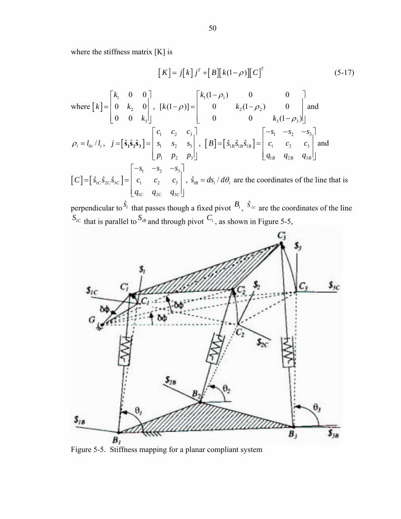
50

where the stiffness matrix [K] is

[ ] [ ] [ ][ ][ ](1 ) TTK j k j B k Cρ= + − (5-17)

where [ ]1

2

3

0 00 00 0

kk k

k

⎡ ⎤⎢ ⎥= ⎢ ⎥⎢ ⎥⎣ ⎦

, 1 1

2 2

3 3

(1 ) 0 0[ (1 )] 0 (1 ) 0

0 0 (1 )

kk k

k

ρρ ρ

ρ

−⎡ ⎤⎢ ⎥− = −⎢ ⎥⎢ ⎥−⎣ ⎦

and

0 /i i il lρ = , [ ]1 2 3

1 2 3

1 2 3

ˆ ˆ ˆc c c

j s s sp p p

⎡ ⎤⎢ ⎥= = ⎢ ⎥⎢ ⎥⎣ ⎦

1 2 3s s s , [ ] [ ]1 2 3

1 1 1 1 2 3

1 2 3

ˆ ˆ ˆB B B

B B B

s s sB s s s c c c

q q q

− − −⎡ ⎤⎢ ⎥= = ⎢ ⎥⎢ ⎥⎣ ⎦

and

[ ] [ ]1 2 3

1 2 3 1 2 3

1 2 3

ˆ ˆ ˆC C C

C C C

s s sC s s s c c c

q q q

− − −⎡ ⎤⎢ ⎥= = ⎢ ⎥⎢ ⎥⎣ ⎦

, ˆ /iB i is ds dθ= are the coordinates of the line that is

perpendicular to is that passes though a fixed pivot iB , ˆ i cs are the coordinates of the line iCS that is parallel to iBS and through pivot iC , as shown in Figure 5-5,

Figure 5-5. Stiffness mapping for a planar compliant system

51

Stiffness Matrix for Spatial Compliant Structures

The analysis of stiffness matrix for the planar structure was presented in the

previous sections. Now the spatial stiffness property will be explored. In this section,

necessary concepts of projective geometry for point and line-vector are provided briefly,

followed by the analysis of a spatial 3-3 octahedron and the desired special 6-6 spatial

parallel manipulator.

In order to perform the analysis, it is essential to expand some of the concepts from

the 2-D plane to 3-D space. In the planar case, the Cartesian coordinate for a point is

defined by two dimensionless scalar values: X and Y, which are also dependent on the

reference point of the selected coordinate system. In Screw theory [Cra01],

homogeneous coordinates (w; x, y, z) are used to describe the location of a point and

i i ii

i

x y zrw

+ +=

i j k refers to the position vector from the reference point O to the point A

with Cartesian coordinate ( , , )i i ix y z . Usually it is assumed that w=1 so that the ratios of

x/w, y/w, z/w are equal to x, y and z. This homogeneous coordinate system also allows

for a point at infinity. When |w|=0, the point A is at infinity in the direction parallel to

( )x y z+ +i j k . For points not at infinity, w is always a non-zero value. To simplify the

expressions in this work, the coordinate of a point will also be expressed as (x, y, z).

It is clear that in the planar case, the equation of a line can be expressed by three

numbers L, M, and R, which are first introduced by Plücker, and are called Plücker line

coordinates. In 3-D space, the ray coordinate of a line is defined by any two distinct

points on the line. The coordinate of point 1 and point 2 are 1 1 1 1( , , )x y zr and

52

2 2 2 2( , , )x y zr respectively. The vector S whose direction is parallel to the line could be

written as:

( )= 2 1S r - r , (5-18) or L M N= + +S i j k (5-19)

So vector S provides directional information for the line segment composed by the

two points. Now consider another vector r from the reference origin to any general point

1 1 1( , , )x y z on the line, the cross product of the two vectors defines a new vector which is

perpendicular to both of the vectors. This is written as

OL = ×S r S . (5-20)

The vector OLS is the moment of the line about the origin O and is clearly origin

dependent, while the vector S provides the directional information for the line. Thus the

coordinate of a line is written as { }OLS;S and this is also called the Plücker coordinates of

the line. The semi-colon in the coordinates indicates that the dimensions of S and OLS are

different, i.e., S is dimensionless while S0L has units of length.

From equation (5-20), the moment vector OLS is:

1 1 1OL x y z P Q RL M N

= = + +i j k

S i j k , (5-21)

where

1 1

1 1

1 1

P y N z LQ z L x NR x M y L

= −= −= −

(5-22)

The Plücker coordinates for the line joining two points with coordinates

( )1 1 11; , ,x y z and ( )2 2 21; , ,x y z was expressed by Grassmann by the six 2×2 determinants of

the array:

53

1 1 1

2 2 2

11

x y zx y z

⎡ ⎤⎢ ⎥⎣ ⎦

(5-23)

as 1

2

11

xL

x= , 1

2

11

yM

y= , 1

2

11

zN

z= , and 1 1

2 2

y zP

y z= , 1 1

2 2

z xQ

z x= , 1 1

2 2

x yP

x y=

The Plücker line coordinates { } { , , ; , , }OL L M N P Q R=S;S are homogeneous since

non-zero scalar multiples of all the coordinates still determine the same line [Cra01]. The

semicolon inside the coordinate separates the (L, M, N) and (P, Q, R) because their

dimensions are different. From equation (5-19), the direction ratios (L, M, N) are related

to the distance |S| by

2 2 2 2| |L M N+ + = S (5-24)

It is useful to unitize these directional values of these homogeneous coordinates to

simplify the application;

2 1 2 1 2 1, ,| | | | | |

x x y y z zL M NS S S− − −

= = = (5-25)

which are also called direction cosines of the lines or unit direction ratios. Therefore, the

new set of L, M, and N has the new restriction

2 2 2 1L M N+ + = . (5-26)

Using the Plücker line coordinates, a force f is expressed as a scalar multiple fS .

The reference point is selected in such a way that the moment of the force f about this

reference point, 0m , can be expressed as a scalar multiple OLfS where OLS is the moment

vector of the line. So the action of the force applied on the body can be expressed as a

scalar multiple of the standard Plucker line coordinates and the coordinates of the force

are:

54

ˆˆ { } { , }OLw f f= ⋅ = = 0S S;S f m , (5-27)

where { }OLS;S is the Plucker line coordinates and 1=S . It is clear that f is a line bound

vector and coordinate independent, while the moment 0m is origin dependent.

For spatial parallel mechanisms, the forward static analysis consists of computing the

resultant wrench ˆ { }w = f;m due to linearly independent forces generated in the legs

acting upon the moving platform. The resultant wrench could be simply expressed:

1 01 2 02 3 03

1 1 01 2 2 02 3 3 03

ˆ { } { } { } { } ...{ ; } { ; } { ; } ...

wf S S f S S f S S= = + + +

= + + +f;m f ;m f ;m f ;m

. (5-28)

Equation (5-28) may be written as

w = jλ , (5-29)

where j is the Jacobian matrix of the structure. The columns of the matrix are composed

of the Plücker coordinates of the lines of the leg connector forces as

1 2 3

01 02 03

...

...S S SS S S

⎡ ⎤= ⎢ ⎥

⎣ ⎦j . (5-30)

λ is the column vector with the scalar of the forces as its elements.

1

2

3

...

fff

λ

⎡ ⎤⎢ ⎥⎢ ⎥=⎢ ⎥⎢ ⎥⎣ ⎦

. (5-31)

55

Figure 5-6. 3-D Model for special 6-6 parallel mechanism

Figure 5-7. Top view of the special 6-6 configuration

56

Now consider the proposed special 6-6 parallel passive structure, its 3-D model and

plan view are shown in Figures 5-6 and 5-7.

This special 6-6 spatial parallel manipulator has a moveable top platform connected

to the fixed platform (ground) by six translational springs acting in-parallel. Each leg has

a conventional spring as the compliant component and as acting in the prismatic joint of

spherical-prismatic-spherical serial chain. The parallel manipulator with six such

compliant legs as well as one top platform and one base platform thus has six degrees of

freedom.

The top platform is connected to the base platform by the initially unloaded

compliant coupling which restricts any relative spatial motion between the bodies. The

corresponding stiffness mapping is thus a one-to-one correspondence that associates a

twist describing the relative displacement between the top and base platform with the

corresponding resultant wrench provided by the springs between them.

The basic shapes of the top platform and the base platform of this special

configuration are equilateral triangles with the top and base triangle side lengths being a

and b respectively while pa and pb are the joints separation distance between the pivots.

The distance h between the geometrical center of the top platform and the geometrical

center of the base platform is selected in such a way that it is qualify the following

expression based on the analysis in the previous chapters:

2bh a= = . (5-32)

The top platform has 6 spherical pivot points 1, 1, 1, 1, 1, 1A B C D E F located along its

triangle sides and the base platform has 6 spherical pivot points , , , , ,A B C D E F along its

triangle sides. The six springs are connected respectively and in order to simplify the

57

process of the analysis, it is necessary to establish the geometry of the system. The

following are position vectors that define the directions of the six legs and their

magnitudes define the lengths of the six legs:

1 1 1 2 1 1

3 1 1 4 1 1

5 1 1 6 1 1

,

,

,

l AA OA OA l BB OB OB

l CC OC OC l DD OD OD

l EE OE OE l FF OF OF

= = − = = −

= = − = = −

= = − = = −

uuur uuur uuur uuur uuur uuur

uuuur uuuur uuur uuuur uuuur uuur

uuur uuuur uuur uuur uuur uuur. (5-33)

One coordinate system is attached to the base platform, which is fixed to ground,

with the z axis pointing upwards to the top platform. The origin of the coordinate system

is located right on the geometrical center of the base triangle platform.

Now considering some external wrench is applied on the top platform and the

whole system is in static equilibrium with the six spring forces as the moving top

platform twists relative to the fixed base platform. Here a wrench [ ]w = 0f;m can be

thought of as a force[ ]f;0 acting though the origin together with a general couple[ ]00;m ,

adding these sets of coordinates together reproduces the original wrench coordinates.

Similar to the wrench, a twist (written in axial coordinates) can be thought of as a rotation

[ ]0,φ about a line through the origin together with a general translation [ ]X,0 , adding

these sets of coordinates together reproduces the original six twist coordinates:

[ ]D = X,φ .[Gri91A]

In order to maintain the system equilibrium, the top platform moves as the external

wrench changes. The incremental change of wrench may be written as [ ]ˆ ;wδ δ δ= f m ,

and the form of the desired stiffness mapping of the compliant structure may be written

as

58

[ ] ˆw K Dδ δ= , (5-34)

where [ ]K is the 6×6 stiffness matrix, which relates the incremental twist

( [ ]ˆ ,D Xδ δ δφ= ) of the top platform relative to the fixed base platform/ground to the

incremental change of the wrench.

As it is specified in the previous chapters, the geometrical properties of the

platform are known: the leg lengths are measured, while the dimensional values of the

top and base triangles are invariant and pre-defined. The individual spring constants of

the springs are also known.

In order to determine the mapping of (5-34), it is necessary to first differentiate (5-

29) [Pig98], which could also be written as

1 1 01

2 2 02

3 3 03

4 4 04

5 5 05

6 6 06

( )( )( )

ˆ( )( )( )

k l lk l lk l l

wk l lk l lk l l

−⎡ ⎤⎢ ⎥−⎢ ⎥⎢ ⎥−⎡ ⎤

= = = ⎢ ⎥⎢ ⎥ −⎣ ⎦ ⎢ ⎥⎢ ⎥−⎢ ⎥

−⎢ ⎥⎣ ⎦

0

fjλ j

m, (5-35)

where ik is the individual spring constant of the thi spring, and 0,i il l are the current length

and free length of the thi spring respectively, so that 0( )i i ik l l− is the force in the thi leg due

to the extension of the thi spring. The Jacobian matrix j is:

1 2 3 4 5 6

1 2 3 4 5 6

⎡ ⎤= ⎢ ⎥× × × × × ×⎣ ⎦

S S S S S Sj

OA S OB S OC S OD S OE S OF S , (5-36)

where, iS is the direction cosine of the axial line of the thi leg. These direction cosines

could be calculated and unitized via (5-25):

59

1 2 3 4 5 61 2 3 4 5 6

1 1 1 1 1 1, , , , ,l l l l l l

= = = = = =AA BB CC DD EE FFS S S S S S

The lower three rows of the 6×6 matrix in (5-36) are the moments of the six lines

relative to the reference point O. Because OA, OB, OC, OD, OE and OF are all fixed

line vectors on the base platform triangle, and are constant, this matrix is solely a

function of the direction cosines of the six legs.

The differential of equation (5-35) is expressed as

1 1

2 2

1 2 3 4 5 6 3 3

1 2 3 4 5 6 4 4

5 5

6 6

1 1 01

2 2 02

1 2 3 4 5 6 3 3 03

1 2 3 4 5 6

( )( )(

k lk l

S S S S S S k lOA S OB S OC S OD S OE S OF S k l

k lk l

k l lk l l

S S S S S S k l lOA S OB S OC S OD S OE S OF S

δδδδδδ

δ δ δ δ δ δδ δ δ δ δ δ

⎡ ⎤⎢ ⎥⎢ ⎥⎢ ⎥⎡ ⎤ ⎡ ⎤

= ⎢ ⎥⎢ ⎥ ⎢ ⎥× × × × × ×⎣ ⎦ ⎣ ⎦ ⎢ ⎥⎢ ⎥⎢ ⎥⎢ ⎥⎣ ⎦

−−−⎡ ⎤

+ ⎢ ⎥× × × × × ×⎣ ⎦

o

δfδm

4 4 04

5 5 05

6 6 06

)( )( )( )

k l lk l lk l l

⎡ ⎤⎢ ⎥⎢ ⎥⎢ ⎥⎢ ⎥−⎢ ⎥⎢ ⎥−⎢ ⎥

−⎢ ⎥⎣ ⎦

(5-37) Here ilδ is related to Dδ by the following expression:

[ ] ˆTl Dδ δ= j (5-38)

where [ ]j is the Jacobian matrix of the parallel structure. The column of this 6×6 matrix

is the line coordinates of the thi leg [Gri91A].

Griffis demonstrated that in order to relate iSδ with Dδ , each leg needs to have two

derivatives, which are perpendicular to the axis of that leg at its base point, to describe

the iSδ . Because each leg is individually connected to the base platform and top

platform via a ball joint and a hook joint, it only possess two degrees of freedom: two

60

rotations whose rotation axis are mutual perpendicular. Griffis also provides the stiffness

mapping analysis for a 3-3 octahedral spatial platform: the analysis is based on Screw

theory and utilizes some geometrical restrictions and configurations of the octahedral

structure. Three examples include that two legs sharing one concentric ball joint at one

fixed pivot, four legs sharing one triangle side and the pivots are located on the vertexes

of the triangles. Although the analysis result is exclusively for the 3-3 octahedral

mechanism, the conceptual approach is applicable to the general spatial stiffness analysis.

The stiffness mapping of the special 6-6 parallel manipulator is determined by following

the same procedure.

The general expression of the stiffness matrix for the special 6-6 parallel platform

is presented as

[ ] [ ][ ][ ] [ ][ ][ ] [ ][ ][ ][ ][ ][ ] [ ][ ][ ]

(1 ) (1 )

(1 ) (1 )

T T Ti i i i i

T Ti i i i

K k k k

k V k V

α α

θ α α

δ ρ δ δ ρ δ

δ ρ δ ρ

= + − + −

+ − + −

θ θ

θ

j j j j j j

j j, (5-39)

where [ ] 1 2 3 4 5 6

1 2 3 4 5 6

⎡ ⎤= ⎢ ⎥× × × × × ×⎣ ⎦

S S S S S Sj

OA S OB S OC S OD S OE S OF S (5-40)

[ ]

1

2

3

4

5

6

0 0 0 0 00 0 0 0 00 0 0 0 00 0 0 0 00 0 0 0 00 0 0 0 0

i

kk

kk

kk

k

⎡ ⎤⎢ ⎥⎢ ⎥⎢ ⎥

= ⎢ ⎥⎢ ⎥⎢ ⎥⎢ ⎥⎢ ⎥⎣ ⎦

[ ]

1 1

2 2

3 3

4 4

5 5

6 6

(1 ) 0 0 0 0 00 (1 ) 0 0 0 00 0 (1 ) 0 0 0

(1 )0 0 0 (1 ) 0 00 0 0 0 (1 ) 00 0 0 0 0 (1 )

i i

kk

kk

kk

k

ρρ

ρρ

ρρ

ρ

−⎡ ⎤⎢ ⎥−⎢ ⎥⎢ ⎥−

− = ⎢ ⎥−⎢ ⎥⎢ ⎥−⎢ ⎥

−⎢ ⎥⎣ ⎦

(5-41)

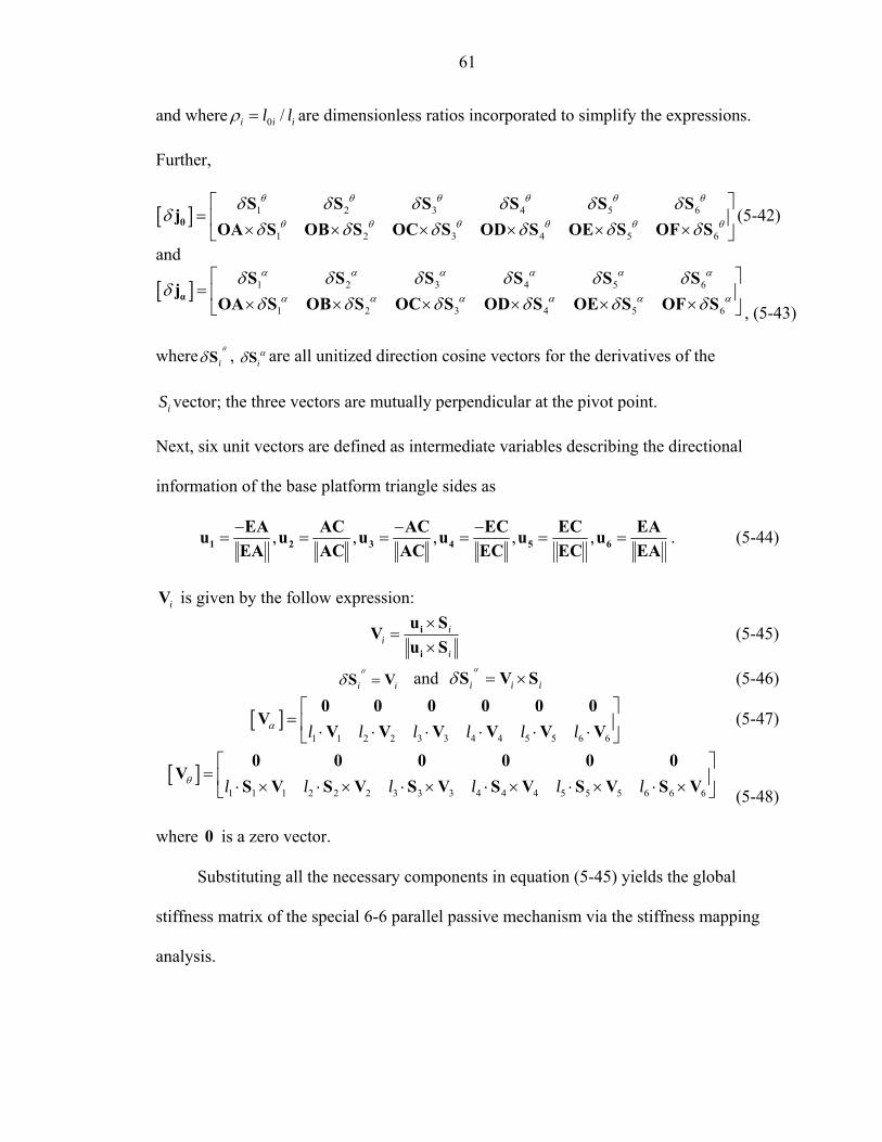
61

and where 0 /i i il lρ = are dimensionless ratios incorporated to simplify the expressions.

Further,

[ ] 1 2 3 4 5 6

1 2 3 4 5 6

θ θ θ θ θ θ

θ θ θ θ θ θ

δ δ δ δ δ δδ

δ δ δ δ δ δ⎡ ⎤

= ⎢ ⎥× × × × × ×⎣ ⎦θ

S S S S S Sj

OA S OB S OC S OD S OE S OF S(5-42)

and

[ ] 1 2 3 4 5 6

1 2 3 4 5 6

α α α α α α

α α α α α α

δ δ δ δ δ δδ

δ δ δ δ δ δ⎡ ⎤

= ⎢ ⎥× × × × × ×⎣ ⎦α

S S S S S Sj

OA S OB S OC S OD S OE S OF S , (5-43)

where i

θ

δS , iαδS are all unitized direction cosine vectors for the derivatives of the

iS vector; the three vectors are mutually perpendicular at the pivot point.

Next, six unit vectors are defined as intermediate variables describing the directional

information of the base platform triangle sides as

, , , , ,− − −= = = = = =1 2 3 4 5 6

EA AC AC EC EC EAu u u u u uEA AC AC EC EC EA

. (5-44)

iV is given by the follow expression:

ii

i

×=

×i

i

u SVu S

(5-45)

i i

θ

δ =S V and i i i

α

δ = ×S V S (5-46)

[ ]1 1 2 2 3 3 4 4 5 5 6 6l l l l l lα

⎡ ⎤= ⎢ ⎥⋅ ⋅ ⋅ ⋅ ⋅ ⋅⎣ ⎦

0 0 0 0 0 0V

V V V V V V (5-47)

[ ]1 1 1 2 2 2 3 3 3 4 4 4 5 5 5 6 6 6l l l l l lθ

⎡ ⎤= ⎢ ⎥⋅ × ⋅ × ⋅ × ⋅ × ⋅ × ⋅ ×⎣ ⎦

0 0 0 0 0 0V

S V S V S V S V S V S V (5-48)

where 0 is a zero vector.

Substituting all the necessary components in equation (5-45) yields the global

stiffness matrix of the special 6-6 parallel passive mechanism via the stiffness mapping

analysis.

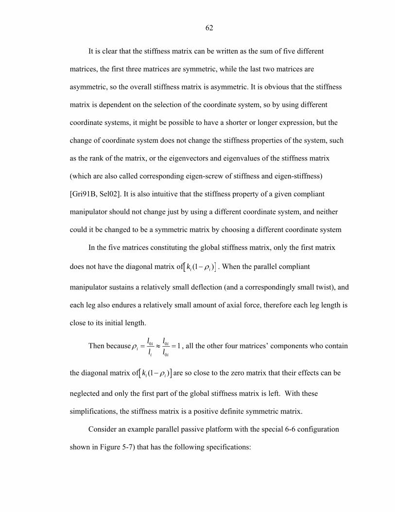
62

It is clear that the stiffness matrix can be written as the sum of five different

matrices, the first three matrices are symmetric, while the last two matrices are

asymmetric, so the overall stiffness matrix is asymmetric. It is obvious that the stiffness

matrix is dependent on the selection of the coordinate system, so by using different

coordinate systems, it might be possible to have a shorter or longer expression, but the

change of coordinate system does not change the stiffness properties of the system, such

as the rank of the matrix, or the eigenvectors and eigenvalues of the stiffness matrix

(which are also called corresponding eigen-screw of stiffness and eigen-stiffness)

[Gri91B, Sel02]. It is also intuitive that the stiffness property of a given compliant

manipulator should not change just by using a different coordinate system, and neither

could it be changed to be a symmetric matrix by choosing a different coordinate system

In the five matrices constituting the global stiffness matrix, only the first matrix

does not have the diagonal matrix of[ ](1 )i ik ρ− . When the parallel compliant

manipulator sustains a relatively small deflection (and a correspondingly small twist), and

each leg also endures a relatively small amount of axial force, therefore each leg length is

close to its initial length.

Then because 0 0

0

1i ii

i i

l ll l

ρ = ≈ = , all the other four matrices’ components who contain

the diagonal matrix of[ ](1 )i ik ρ− are so close to the zero matrix that their effects can be

neglected and only the first part of the global stiffness matrix is left. With these

simplifications, the stiffness matrix is a positive definite symmetric matrix.

Consider an example parallel passive platform with the special 6-6 configuration

shown in Figure 5-7) that has the following specifications:

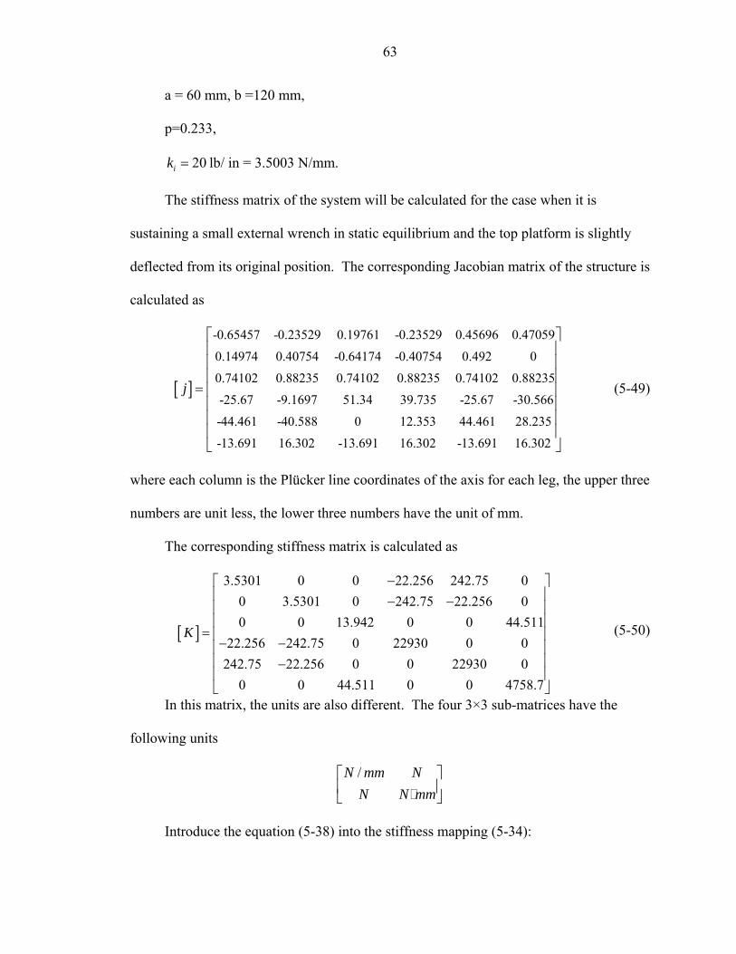
63

a = 60 mm, b =120 mm,

p=0.233,

20ik = lb/ in = 3.5003 N/mm.

The stiffness matrix of the system will be calculated for the case when it is

sustaining a small external wrench in static equilibrium and the top platform is slightly

deflected from its original position. The corresponding Jacobian matrix of the structure is

calculated as

[ ]

-0.65457 -0.23529 0.19761 -0.23529 0.45696 0.470590.14974 0.40754 -0.64174 -0.40754 0.492 00.74102 0.88235 0.74102 0.88235 0.74102 0.88235-25.67 -9.1697 51.34 39.735 -25.67 -30.566-44.461 -40.588 0 12.353 44.461 28.235-13.6

j =

91 16.302 -13.691 16.302 -13.691 16.302

⎡ ⎤⎢ ⎥⎢ ⎥⎢ ⎥⎢ ⎥⎢ ⎥⎢ ⎥⎢ ⎥⎣ ⎦

(5-49)

where each column is the Plücker line coordinates of the axis for each leg, the upper three

numbers are unit less, the lower three numbers have the unit of mm.

The corresponding stiffness matrix is calculated as

[ ]

3.5301 0 0 22.256 242.75 00 3.5301 0 242.75 22.256 00 0 13.942 0 0 44.511

22.256 242.75 0 22930 0 0242.75 22.256 0 0 22930 0

0 0 44.511 0 0 4758.7

K

−⎡ ⎤⎢ ⎥− −⎢ ⎥⎢ ⎥

= ⎢ ⎥− −⎢ ⎥⎢ ⎥−⎢ ⎥⎣ ⎦

(5-50)

In this matrix, the units are also different. The four 3×3 sub-matrices have the

following units

/N mm NN N mm

⎡ ⎤⎢ ⎥⎣ ⎦

Introduce the equation (5-38) into the stiffness mapping (5-34):

64

[ ] [ ][ ]ˆˆ Tw K D K jδ δ δ−= = l (5-51)

For a given set of minute deflections of the legs, the above equation can be used to

calculate the applied external wrench.

-2.2912 -0.8236 0.69168 -0.8236 1.5995 1.64720.52414 1.4265 -2.2463 -1.4265 1.7222 02.5938 3.0885 2.5938 3.0885 2.5938 3.0885

ˆ-89.852 -32.097 179.7 139.09 89.852 -106.99-155.63 -142.07 0 43.239 155.63 98.832-47.921 57.061 -47

w =

1

2

3

4

5

6.921 57.061 -47.921 57.061

llllll

∆⎡ ⎤⎡ ⎤⎢ ⎥⎢ ⎥ ∆⎢ ⎥⎢ ⎥⎢ ⎥⎢ ⎥ ∆⎢ ⎥⎢ ⎥ ∆⎢ ⎥⎢ ⎥⎢ ⎥⎢ ⎥ ∆⎢ ⎥⎢ ⎥∆⎢ ⎥⎣ ⎦ ⎣ ⎦

(5-52)

If the top platform of the special 6-6 parallel passive platform is deflected much

from its unladed home position, then the compliance matrix can be calculated from

equation (5-39).

65

CHAPTER 6 FORWARD ANALYSIS FOR SPECIAL 6-6 PARALLEL PLATFORM

The kinematic forward analysis is very important to control applications. In this

chapter, the forward kinematic analysis for parallel 3-3 manipulator is introduced. Then

a geometrical method, patented by Duffy and Griffis [Gri93], of determining the

equivalent 3-3 parallel structure for a special 6-6 configuration mechanism is described.

Forward Kinematic Analysis for a 3-3 Platform

It is necessary to determine the position and orientation of the end effector of the

manipulator. Given the geometrical properties of the parallel platform, including leg

length, connector pivots locations and etc., the forward kinematic analysis determines the

relation between the end effector pose and it geometrical properties. As stated in the

previous chapters, the forward kinematic analysis is complicated compared to the reverse

kinematic analysis. This problem is also geometrically equivalent to the problem of

finding out ways to place a rigid body such that six of its given points lie on six given

spheres.

During the late 80’s and early 90’s of last century, many researchers had worked on

the forward kinematic analysis of parallel manipulators. Many different approaches such

as closed-form solutions of special cases, numerical schemes, and analytical approaches

were considered for both special cases and general 6-6 configurations. Hunt [Hun98]

studied the geometry and mobility of the 3-3 in-parallel manipulator. Wen and Liang

[Wen94] used an analytical approach and solved the problem for the 6-6 Stewart platform

with a planar base and platform by reducing of the kinematic equations into a uni-variate

66

polynomial and concluded that the upper bound of the solutions for forward kinematic

problems is 40 for this class. Merlet [Mer92, Mer00] had studied direct kinematic

solutions for general 6-6 parallel platform and special cases with additional sensors.

Various researchers have stated that for a general 6-6 in-parallel platform and with

a given set of fixed leg lengths, it is possible to assemble it in 40 different configurations

[Das00, Hun98]. It is not likely that all of the 40 configurations are real and applicable.

Due to the difficulty of the forward kinematic analysis for the general 6-6 in-parallel

platform, it is worthwhile to consider some special cases with reduced complexity. The

simplest form of this class is first analyzed.

Although there are different configurations and designs for a simple spatial parallel

platform, the symmetric 3-3 parallel platform shown in Figure 6-1 is among the most

important and widely analyzed structures.

This 3-3 parallel platform is also called an “octahedron”. It has eight triangular

faces, six vertices and twelve edges. Four edges are concurrent at each vertex. Every

vertex is contained in four faces. The device has all six degrees of freedom, ignoring the

trivial freedom of each leg rotating about its own axis.

The forward kinematic analysis for the 3-3 in-parallel manipulator was first solved

by Griffis and Duffy [Gri89] who showed that the position and orientation of the top

platform can be determined with respect to the base when given the lengths of the six

connectors as well as the geometry of the connection points on the top and base. The

solution is a closed-form solution and is based on the analysis of the input/output

relationship of three spherical four bar mechanisms. The three spherical four bar

mechanisms (see Figure 6-3) result in three equations in the tan-half angle of the three

67

unknowns θx, θy, and θz. These tan-half angles are simply named x, y, and z. Elimination

of the variables y and z results in the following polynomial which contains the variable x

as its only unknown [Gri89].

Figure 6-1. 3-D drawing of the 3-3 in-parallel platform

21 24α βρ ρΕ = − , (6-1)

where

68

2 2 2 2 2 23 3 2 1 2 3 3 1 2 3 3 1 1 2 3 3 2 1

2 23 3 1 2 1 2 3 3 1 1 2 3 3 2 2 1

2 23 3 1 2 3 3 1 1 1 2 3 3 1 2 1 2

2 2 2 23 3 1 1 2 3 3 2 2 1 3 3 1 2

2 2 23 3 1 2 1 3 3 2 1 3 3

2 4 2 4

2 4 4

8 2 2

4 4 8

2 4 2

A B a c c A B c b A C a c c A C c b

A E a a c c A E a c b A E a c b

A E b b A D c c b b B C a a c c

B C a c b B C a c b B C b b

B E a a c B E a b B D

α = − + −

− + +

− − −

+ + −

+ − − 2 1 1 22 2 2

3 3 1 2 2 3 3 1 2 3 3 1 2 1 22 2 2 2

3 3 1 2 1 2 3 1 2 1 2 3 1 22 2 2 2 2 2 2 2 2

3 1 2 3 1 2 3 1 2

3 3 1 2 3 3 1 2 3 3 1 2

3 3 1 2 3 3 1 2 3 3 1 2

21 1 1 1

22 2 2 2

2 4 2

2

44

a c b b

C E a a c C E a b C D a c b b

D E a a b b D a a c c A c c

B c a C a c E a a

A E b b A D c c D E a aB C b b B D c a C D a c

b a c

b a c

β

ρ

ρ

+ − −

− − −

− − −

= + +− − −

= −

= −

2 21 1 1 1 1 1 1 1

2 22 2 2 2 2 2 2 2

, 0.5 ,

, 0.5 ,

a A x C b D x c B x E

a A x B b D x c C x E

= + = = +

= + = = +

The coefficients ,..., , 1,2,3i iA E i = are expressed in terms of known quantities.

Their values for the generic spherical four bar mechanism shown in Figure 6-2 may be

written as

12 41 34 12 41 34 41 34 12 23 12 41 34

12 41 34 12 41 34 41 34 12 23 12 41 34

12 41 34 12 41 34 41 34 12 23 12 41 34

12 34

12 41 34 12 41 34 41 34 12 23 12 41 34

4

A s c s s s c s s c c c c cB s c s s s c s s c c c c cC s c s s s c s s c c c c cD s sE s c s s s c s s c c c c c

= − − + −= − − + + −= − + − + −= −= + + + −

where sin( )ij ijs α= and cos( )i ic α= . For this problem, the coefficients are obtained by

replacing the vertex as the origin of the three spherical four-bar linkages (shown in Figure

6-3) with points o, p, and q respectively. The corresponding mapping of the angles of the

spherical four-bar linkages is shown in table 6-1.

69

Figure 6-2. A general spherical four-bar mechanism, Griffis [Gri89]

Table 6-1. Mappings of angles of spherical four bar mechanism. Origin o p Q

Output: 12a qor∠ ops∠ pqr∠

Coupler: 23a ros∠ spt∠ tqr∠

Input: 34a sop∠ tpq∠ rqo∠

Ground: 41a poq∠ pqo∠ oqp∠

The resulting solution shown above is an eighth degree polynomial in the square of

one variable which yields a maximum of sixteen solution poses for any given set of

connector lengths and base-top triangles lengths. Eight solutions were reflected about the

70

plane formed by the base connector points. There can be up to 16 real solutions and

therefore, there can be 0,2,4,6 or 8 pairs of real, reflected solutions.

Figure 6-3. 3-3 in-parallel mechanism with three spherical four-bar linkages, Griffis

[Gri89]

Forward Kinematic Analysis for Special 6-6 In-Parallel Platform

The configuration of the special 6-6 in-parallel platform is carefully chosen such

that the forward kinematic analysis can use a method similar to the method for the 3-3 in-

parallel platform. This section will show the geometric relationship between the special

6-6 in-parallel platform and an equivalent 3-3 platform and how to solve the direct

kinematic analysis problem by using this conversion. The relationship between a Special

6-6 platform and its equivalent 3-3 platform was discovered by Griffis and Duffy [Gri93]

and is presented here for completeness as the forward analysis is an important part of the

control algorithm for the force control device developed in this dissertation.

71

A Special 6-6 platform is defined as one which is geometrically reducible to an

equivalent 3-3 platform. Figure 6-4 depicts a perspective and plan view of a 6-6 platform

where the leg connector points R0, S0, and T0 lie along the edges of the triangle defined

by points O0, P0, and Q0 and the leg connector points O1, P1, and Q1 lie along the edges of

the triangle defined by the points R1, S1, and T1. The objective here is to determine the

distance between the pairs of points O0 - R1, O0 - S1, P0 - S1, P0 -T1 , Q0 - T1, and Q0 - R1.

These distances represent the leg connector lengths for an equivalent 3-3 platform.

Throughout this analysis, the notation minj will be used to represent the distance

between the two points Mi and Nj and the notation minj will represent the vector from

point Mi to Nj. Using this notation, the problem statement can be written as:

given: o0o1, p0p1, q0q1, r0r1, s0s1, t0t1 connector lengths for Special 6-6 platform

o0p0, p0q0, q0o0, o0s0, p0t0, q0r0 base triangle parameters

r1s1, s1t1, t1r1, r1o1, s1p1, t1q1 top triangle parameters

find: o0r1, o0s1, p0s1, p0t1, q0t1, q0r1 connector lengths for equivalent 3-3 platform

Obviously it is the case that

s0p0 = o0p0 – o0s0 ; t0q0 = p0q0 – p0t0 ; r0o0 = q0o0 – q0r0

o1s1 = r1s1 – r1o1 ; p1t1 = s1t1 – s1p1 ; q1r1 = t1r1 – t1q1 . (6-2

)

The six leg connectors of the equivalent 3-3 platform define an octahedron, i.e.,

there are eight triangular faces; the top and bottom platform triangles and six faces

defined by two intersecting connectors and an edge of either the base or top platform.

The solution begins by first defining angles β and γ which, for each of the six faces

72

defined by intersecting connectors, defines the angle in the plane between a connector of

the Special 6-6 platform and an edge of either the top or base platform as appropriate.

A

B Figure 6-4. Special 6-6 platform and equivalent 3-3 platform, A) Perspective view, B)

Plan view

Figure 6-5 shows the angles γ1 and β1. The angle γ2 is defined as the angle between

r0r1 and r0o0 and the angle γ3 is defined as the angle between s0s1 and s0o0. Similarly, the

O0

O1

P0

P1

Q0

Q1 R1

R0

S1

S0

T1

T0

O0

O1

P0

P1

Q0

Q1 R1

R0

S1

S0

T1

T0

73

angle β2 is defined as the angle between q1t1 and q1q0 and the angle β3 is defined as the

angle between o1s1 and o1o0.

Figure 6-5. Definition of angles β and γ

Figure 6-6 shows a planar triangle that is defined by the vertex points G1, G2, and

G3. A point G0 is defined as a point on the line defined by G1 and G2 and the angle φ is

shown as the angle between g0g2 and g0g3. The cosine law for the triangle defined by

points G0, G2, and G3 yields

cb2cbcos

2b

22 l−+=ϕ (6-3)

Next consider that the triangle lies in a plane defined by u and v coordinate axes.

The coordinates of any point Gi may then be written as (ui, vi). The distance al may then

be expressed as

P0

Q0

O0

S1

R1 T1

P1

T0

γ1

β1

74

ϕ++=

ϕ++ϕ+ϕ=

ϕ+ϕ+=

−+−=

cosca2cacosca2a)cos(sinc

)sinc()cosca(

)vv()uu(

22

2222

22

213

213

2al

. (6-4)

Figure 6-6. Planar triangle

Substituting (6-3) into (6-4) and simplifying gives

)acabacbab(

b1

)cb(baca

2b

2222

2b

22222a

l

ll

−+++=

−+++= . (6-5)

Regrouping this equation gives

2 2 2 2 2 2( ) ( )( )a bb a a b c ab a b a b c ab+ = + + + = + +l l . (6-6)

The result of equation (6-6) can be applied to each of the six side faces of the

octahedron defined by the leg connectors of the equivalent 3-3 platform. The parameter

substitutions are shown in Table 6-2.

G1 G2 G0

G3

φ

a b

c al bl

u

v

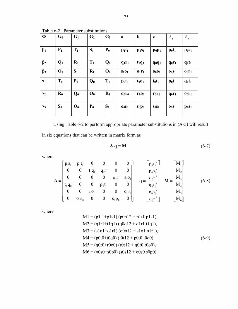
75

Table 6-2. Parameter substitutions Φ G0 G1 G2 G3 a b c al bl

β1 P1 T1 S1 P0 p1t1 p1s1 p0p1 p0t1 p0s1

β2 Q1 R1 T1 Q0 q1r1 t1q1 q0q1 q0r1 q0t1

β3 O1 S1 R1 O0 s1o1 o1r1 o0o1 o0s1 o0r1

γ1 T0 P0 Q0 T1 p0t0 t0q0 t0t1 p0t1 q0t1

γ2 R0 Q0 O0 R1 q0r0 r0o0 r0r1 q0r1 o0r1

γ3 S0 O0 P0 S1 o0s0 s0p0 s0s1 o0s1 p0s1

Using Table 6-2 to perform appropriate parameter substitutions in (A-5) will result

in six equations that can be written in matrix form as

A q = M , (6-7)

where

⎥⎥⎥⎥⎥⎥⎥⎥

⎦

⎤

⎢⎢⎢⎢⎢⎢⎢⎢

⎣

⎡

=

⎥⎥⎥⎥⎥⎥⎥⎥

⎦

⎤

⎢⎢⎢⎢⎢⎢⎢⎢

⎣

⎡

=

⎥⎥⎥⎥⎥⎥⎥⎥

⎦

⎤

⎢⎢⎢⎢⎢⎢⎢⎢

⎣

⎡

=

6

5

4

3

2

1

210

210

210

210

210

210

0000

0000

0000

1111

1111

1111

MMMMMM

rosotqrqsptp

0ps00so0rq00or00

00tp00qtosro000000rqqt000000tpsp

MqA (6-8)

where

M1 = (p1t1+p1s1) (p0p12 + p1t1 p1s1),M2 = (q1r1+t1q1) (q0q12 + q1r1 t1q1),M3 = (s1o1+o1r1) (o0o12 + s1o1 o1r1),M4 = (p0t0+t0q0) (t0t12 + p0t0 t0q0),M5 = (q0r0+r0o0) (r0r12 + q0r0 r0o0),M6 = (o0s0+s0p0) (s0s12 + o0s0 s0p0).

(6-9)

76

Then these equations are manipulated such that dividing the first rows of A and

M by p1t1+p1s1= s1t1, the second rows by q1r1+t1q1= r1t1, and so on to obtain

A q M′ ′= , (6-10)

where

⎥⎥⎥⎥⎥⎥⎥⎥

⎦

⎤

⎢⎢⎢⎢⎢⎢⎢⎢

⎣

⎡

++++++

=′

⎥⎥⎥⎥⎥⎥⎥⎥

⎦

⎤

⎢⎢⎢⎢⎢⎢⎢⎢

⎣

⎡

−−

−−

−−

=′

00002

10

00002

10

00002

10

11112

10

11112

10

11112

10

0100000100

0000110000

0010000001

pssossorrqrrqttpttroosooqtrqqqsptppp

ssrr

ttww

qqpp

MA

with

00

00

0000

00

11

11

1111

11

00

00

0000

00

11

11

1111

11

00

00

0000

00

11

11

1111

11

poos

psosos

ssrro

sororo

w

oqqr

orqrqr

rtrtq

rqtqtq

q

qppt

qtptpt

ttssp

tpspsp

p

=+

==+

=

=+

==+

=

=+

==+

=

Note that 1,,,,,0 ≤≤ srtwqp .

The matrix A′ is dimensionless and depends only on the ratios of where the

connections occur along the sides of the upper and lower bases. Matrix A′ is also

independent of the shapes of the upper and lower triangles. Now all the terms in matrix

A′ are known as they are dimensionless ratios expressed in terms of given distances of

the top and bottom platform. All the terms in vector M ′ are also known as they are

expressed in terms of given dimensions as well as the square of the lengths of the six leg

connectors of the Special 6-6 platform. Thus the square of the lengths of the connectors

for the equivalent 3-3 platform may be determined as:

77

1q A M− ′= (6-11)

Further more, the determinant of A′ is:

pqwtrssrtwqp −−−−−−−= )1)(1)(1)(1)(1)(1()det(A (6-12)

It is interesting to note that the matrix A′ is singular if and only if the following

condition is satisfied:

11

00

11

00

11

00

11

00

11

00

11

00

tptp

soso

rqrq

roro

qtqt

psps

= (6-13)

One case where this could happen would be if all the middle connector pointes S0,

T0, R0, O1, P1, and Q1 are located at the midpoints of the sides of the upper and lower

triangles. We can also conclude that for A′ to be singular, if some of the parameters

srtwqp ,,,,, are less than ½ then some of the other parameters must be greater than ½.

Thus we immediately conclude that if all of the parameters are less than ½ (as is the case

in Figure A-1), then A′ is non-singular. The same statement of course is true if all the

parameters are greater than ½.

Once the leg length dimensions of the equivalent 3-3 platform are determined, the

forward analysis of the 3-3 device as described in Section 6.1 is used to determine the

position and orientation of the top platform relative to the base

78

CHAPTER 7 RESULTS AND CONCLUSION

In this chapter, the individual components of the designed manipulator are tested to

validate the machine design and theoretical analysis presented in the previous chapters.

In order to calibrate each leg’s stiffness, first the force sensor is calibrated. An optical

encoder measures the compliant displacement of the leg and the load cell records the

applied force. The force-displacement relationship is provided for each leg and the

results are analyzed. The parallel platform is then assembled for the 6 DOF wrench

measuring testing. Several experiments are presented and the results are analyzed. At

the end of this chapter, a summary of the work is followed by conclusions and future

work suggestions.

Calibration Experiment for the Force Sensor

In order to get the force/ displacement relationship of the compliant connectors, the

detected force signal and the corresponding displacement signal should be recorded

simultaneously during the individual leg calibration experiment.

A load cell is used to measure the axial force applied on the individual leg. The

rated capacity of the load cell is 5 lb, (22.246 N) and the output of the load cell is an

analog voltage signal, ranging from -5~+5 Vdc. The rated output is 2mV/V ± 20%. It is

necessary to calibrate the load cell first to ensure the validity and accuracy of the

following experiments’ results.

79

0 5 10 15 20 25-1

0

1

2

3

4

5

6

Input Force - (Ns)

Out

put V

olta

ge -

(Vol

ts)

Load cell linearity calibration experiment plot

Figure 7-1. Load cell calibration experiment

0 2 4 6 8 10 12 14-0.5

0

0.5

1

1.5

2

2.5

3

3.5

Input Force - (Ns)

Out

put V

olta

ge -

(Vol

ts)

Load cell linearity calibration experiment plot: Fine plot

Figure 7-2. Load cell calibration experiment - opposite direction

80

The load cell output analog signal is connected to an A/D port of a multi-functional

I/O board and the value of the voltage is recorded with the corresponding known force,

which is provided by a set of standard weights for accurate force calibration. The

mapping of the force/voltage relationship is shown in Figure 7-1 and Figure 7-2.

Five additional sets of experimental data were analyzed and the plots are very

similar, so only one plot is shown here. The linear equation that relates the applied force

to the measured voltage can be written as

1y k x= , (7-1)

where the coefficient k1 is determined to equal 0.00225 Volt/gram. The linear regression

statistics are shown in Table 7-1.

Table 7-1. Load cell regression statistics Regression Statistics

Multiple R 0.999115584 R Square 0.998231949

Adjusted R Square 0.966981949 Standard Error 0.059572297(V)

From the table and the figure above, the load cell shows very high linearity and is

adequate to be used in the following experiments.

Individual Leg Calibration Experiment

After calibrating the load cell, it is necessary to calibrate the compliant connectors

and identify the stiffness property for each of them. During the experiment, the

compliant connector is fixed vertically and is attached to the load cell in such a way that

the applied external force causing either elongation or compression can be detected

properly. The two physical quantities, force and displacement, are detected by the load

81

cell and the optical encoder. The optical encoder is attached on the compliant leg both

for the calibration experiment and for the designed operation.

Axial force is applied on the top of the compliant leg with variable magnitude and

direction in order to get the stiffness mapping of the leg for both compression and

elongation. The resolution of the optical encoder is 1000 counts/inch.

The individual plot of the stiffness mapping for each of the six leg connectors is

shown in Figures 7-3 through 7-8.

-2 -1 0 1 2 3 4 5-5

0

5

10

15Leg 1 Calibration: Force Vs. Displacement

X - Displacement (mm)

Y -

Forc

e (N

)

Figure 7-3. Calibration plot for leg-1

82

-2 -1 0 1 2 3 4 5-6

-4

-2

0

2

4

6

8

10

12



Y -

Forc

e (N

)


-2 -1 0 1 2 3 4 5-5

0

5

10



Y -

Forc

e (N

)


83

-2 -1 0 1 2 3 4 5-6

-4

-2

0

2

4

6

8

10

12



Y -

Forc

e (N

)


-2 -1 0 1 2 3 4 5 6-6

-4

-2

0

2

4

6

8

10

12

14

Leg 5 Calibration: Force Vs. Displacement


Y -

Forc

e (N

)

Figure 7-7 Calibration plot for leg-5

84

-2 -1 0 1 2 3 4 5-6

-4

-2

0

2

4

6

8

10

12



Y -

Forc

e (N

)

Figure 7-8 Calibration plot for leg-6

In the calibration plots, the displacement is measured in mm and force measured in

Newtons. In the original data file, the displacement at each sample time is recorded as

encoder counts and the force is recorded as digitized voltage value. Then the units are

converted by the load cell calibration experiment results together with the following

conversion equations:

1 25.4

453.6 4.448in mmlb gram

= 1 = = Ν

(7-2)

Then, the data in the plots is used to build six individual look-up tables of

displacement vs. force for each leg. During operation, the relative displacement is

measured and the corresponding force value is obtained from the look-up table. These

calibration tables can also be replaced by linear regression of the data for less-accurate

operations, and thus a “linear spring constant” is assigned to each leg.

85

Parallel Platform Force/Wrench Testing Experiment

The force/torque sensor has been factory calibrated, so only the resolution is listed

here. The resolutions for force and torque are shown in the table below

Table 7-2. Force-torque Sensor Resolution

The parallel platform is attached on the top of the force/torque sensor as shown in

Figure 7-9 and its mass center is carefully balanced such that its weight is directly over

the origin of the sensor’s reference coordinate system. This coordinate system is based

on the force/torque sensor, so there is no moment introduced. This z-direction bias force

is easily eliminated in the sampling program, so it will not be discussed further.

Figure 7-9. Photo of the testing experiment for the parallel platform

Fx Fy Fz Tx Ty Tz 0.1 (N) 0.1 (N) 0.2 (N) 5 (N-mm) 5 (N-mm) 5 (N-mm)

86

The home position refers to the position of the platform when it is attached with the

force/torque sensor and placed horizontally, with no other force applied on the top

platform or any leg. The home position is also called the initial position/ orientation, and

it can be specified by its relative displacement from the encoder’s indexed position.

Before use, it is necessary to home the device. This is done by applying some small

force/ wrench to the top platform, so each leg pass through its index position. Thus after

homing, the current position and orientation can be accurately measured even when it is

not in its home position.

Repeatability test

It is important to know the repeatability of the manipulator. The previous

prototype, built by Tyler [Dwa00], did not have good repeatability. Significant friction in

the spherical joints was noted when an external force was applied and then removed.

This friction impacted the ability of the top platform to return repeatedly to the same

home position when external loading was removed.

In order to test its repeatability, two sets of experiment are performed.

1. Apply random force/wrench to the top plate and then remove it, measure the unloaded position/ orientation via the leg lengths measurements

2. Apply a weight of 500 grams on the top plate several times, and compare the measured leg lengths.

Table 7-3. Repeatability experiment, method 1 (Encoder Counts)

Test Number Leg 1 Leg 2 Leg 3 Leg 4 Leg 5 Leg 6

#1 -1 0 0 0 0 -1 #2 0 0 -1 1 2 -1 #3 -6 0 -4 -6 1 -3 #4 -5 2 0 -4 3 -1 #5 -3 -3 -1 -1 -2 -1 #6 -2 0 -1 0 2 2

Average -2.83333 -0.16667 -1.16667 -1.66667 1 -0.83333 STD 2.316607 1.602082 1.47196 2.73252 1.788854 1.602082

87

Table 7-4. Repeatability experiment, method 2 (Encoder Counts) Test

Number Leg 1 Leg 2 Leg 3 Leg 4 Leg 5 Leg 6

#1 -200 -64 -5 -103 101 98 #2 -202 -65 -5 -104 101 100 #3 -207 -66 -5 -104 101 102 #4 -197 -63 -4 -100 100 97 #5 -203 -66 -5 -102 101 98 #6 -202 -65 -4 -103 100 101

Average -201.833 -64.8333 -4.66667 -102.667 100.6667 99.33333 STD 3.311596 1.169045 0.516398 1.505545 0.516398 1.966384

The experiment results are shown in Tables 7-3 and 7-4. The numbers in the

column shows the encoder counts when there is no external load applied (for method 1)

and when the external load is applied on the platform (for method 2). The overall

repeatability for the parallel platform is reasonable.

Forward analysis verification

The forward kinematic analysis was presented in Chapter 5. An experiment is

shown here to validate the analysis result and also to provide for the static analysis

process.

The parallel platform has some external wrench applied on the top plate. The

counts of the relative displacement for each leg is then recorded. Table 7-5 shows the

lengths of the six leg connectors, both in units of encoder counts from the unloaded

position and in units of mm, with the external wrench applied.

The table also shows the calculated lengths of the six connectors of the equivalent

3-3 platform. After performing the forward analysis of the equivalent 3-3 platform, a

reverse analysis of the special 6-6 platform is conducted to calculate the leg lengths and

to verify the forward analysis result.

88

Table 7-5. Forward analysis Leg 1 Leg 2 Leg 3 Leg 4 Leg 5 Leg 6

Encoder Counts -15 -10 -2 -13 -26 -19 Leg length for special 6-6

(measured) (mm) 80.588 67.746 80.918 67.669 80.308 67.517

Leg length for the equivalent 3-3 platform

(mm) 84.595 84.829 84.722 84.145 84.469 80.588

Leg length for the 6-6 platform (reverse analysis)

(mm) 80.587 67.746 80.918 67.669 80.309 67.517

From the table, it is clear that the forward analysis is very accurate, the leg lengths

calculated from the reverse analysis, which are also based on the results of the forward

kinematic analysis, are very close to the leg length values measured by the optical

encoder.

The coordinate systems of the parallel platform are shown in Figure 7-10. The base

points are 0 0, ,O P and 0Q , the origin of the base coordinate system is at point 0O , 0P is on

the X axis, and 0Q is on the XY plane. This coordinate system is fixed in the base. The

top plate corner points are 1 1 1, ,R S T , the origin of the top platform coordinate system is at

point 1R , 1S is on the x axis, and 1T is in the xy plane.

After finding the leg lengths of the equivalent 3-3 platform by the geometrical

conversion, the position and orientation of the platform can be calculated by the forward

kinematic analysis. The detail of this analysis is presented in Chapter 6, so only the

results are presented here.

89

For the measured leg lengths listed in Table 7-5, the forward analysis has only 8

solutions.1 Four are above the base and four are reflected through the base. The four

configurations above the base are discussed here. Each solution can be represented by a

4 4× transformation matrix. The first three elements in the fourth column have units of

length (mm) and all other elements are dimensionless. From now on, the units for the

element in the transformation matrices are omitted. The four calculated transformation

matrices that relate the top and base coordinate systems are

basetop 1

0.5105 0.1095 0.8529 29.20290.8598 0.0718 0.5055 52.4117

0.0059 0.9914 0.1308 59.44080 0 0 1

−⎡ ⎤⎢ ⎥− −⎢ ⎥=⎢ ⎥− −⎢ ⎥⎣ ⎦

T ,

basetop 2

0.5021 0.8648 0.0007 29.71070.8648 0.5020 0.0007 52.1185

0.0058 0.0042 0.9999 59.44690 0 0 1

⎡ ⎤⎢ ⎥−⎢ ⎥=⎢ ⎥−⎢ ⎥⎣ ⎦

T ,

basetop 3

0.4987 0.8668 0.0061 29.91490.1211 0.0627 0.9907 52.00060.8583 0.4947 0.1363 59.4478

0 0 0 1

⎡ ⎤⎢ ⎥− −⎢ ⎥=⎢ ⎥− −⎢ ⎥⎣ ⎦

T , (7-3)

basetop 4

0.3526 0.3757 0.8570 80.99280.3670 0.7869 0.4960 22.5108

0.8608 0.4894 0.1396 8.15100 0 0 1

− −⎡ ⎤⎢ ⎥−⎢ ⎥=⎢ ⎥−⎢ ⎥⎣ ⎦

T .

Although all four solutions are real and satisfy the geometrical conditions, there is

only one solution that corresponds to the actual current configuration. With these

transformation matrices, the coordinates of all points of the 3-3 structure can be

determined. Then drawings of these configurations (or the numerical determination of

1 In general, the forward analysis of the special 6-6 platform will yield 16 possible solutions, 8 above the base and 8 reflections through the base. However for the measured set of leg lengths, only 8 real solutions exist, 4 above the base and 4 reflections through the base.

90

the configuration closest to the most previous pose) can be used to choose the correct

solution set.

Figure 7-10. Coordinate systems of the parallel platform

Here the geometrical meanings of the 4 4× transformation matrices are used to

make the selection. By using homogeneous coordinates, the 4 4× transformation matrix

can be represented as

0

0 0 0 1

A AB BA

B

⎡ ⎤= ⎢ ⎥

⎢ ⎥⎣ ⎦

R PT , (7-4)

where

0

ABP is the location of the origin of the B coordinate system measured with respect

to the A coordinate system, A A A AB B B B⎡ ⎤= ⎣ ⎦R X Y Z , its columns vectors are the

orientation of the B coordinate system measured with respect to the A coordinate system.

O0

O1

P0

P1

Q0

Q1 R1

R0

S1

S0

T1

T0

X

Z

Y

z

x y

91

So by comparing the columns of the transformation matrices, the right solution can be

properly selected.

The transformation matrix for the home position is given below as

basetop home

0.5056 0.8628 0 29.66510.8628 0.5056 0 52.1547

0 0 1 59.99870 0 0 1

⎡ ⎤⎢ ⎥−⎢ ⎥=⎢ ⎥⎢ ⎥⎣ ⎦

T (7-5)

Clearly, the second solution is the correct one since physically the Z axis of the top

coordinate system remained relatively parallel to the Z axis of the base coordinate system

after the loading was applied. For all other solutions, the coordinate systems have too

much rotation relative to the base coordinates system.

Wrench and force testing.

After choosing the correct transformation matrix, the coordinates of all points are

known and the Jacobian matrices of the structure at any instant be calculated. Using the

equilibrium condition, the following equation can be used to calculate the applied force/

wrench as stated in the previous chapters.

w = jλ . (7-6) Numerical example:

In order to verify the accuracy of the PCCFC, several numerical experiments have

been done. For each set of experiment data, the external wrench applied on the top

platform of the PCCFC is measured by the force/torque sensor on which the device is

mounted for this experiment and compared to the calculated wrench based on the sensed

leg lengths. The force/torque sensor date is reported in terms of the sensor’s coordinate

system and the calculated wrench is calculated in terms of the base coordinate system.

The wrenches are compared by converting the calculated wrench to the sensor coordinate

92

system. It is important to note that the force/torque sensor has a left-handed coordinate

system. That is its Z-axis and X-axis are parallel to the corresponding axes of the base

coordinate system of the PCCFC, but the Y-axes are anti-parallel.

The sensor coordinate system is used as the common reference system and the

coordinates of the external wrench detected by the PCCFC are transformed by the

following equation:

2 2 1 1 1 10 0{ ; } { ; }= − ×S S S S p S (7-7)

where superscript 1 and 2 refer to the Screw coordinates in the former coordinate system

and new coordinate system respectively, 1p refers the coordinates of origin of the second

coordinate system in terms of the first coordinate system. This transformation will

determine the calculated wrench in terms of a right-handed coordinate system whose

origin is at the origin of the sensor coordinate system. The x and z axes will be parallel to

the x and z axes of the sensor coordinate system, but the y axis will be anti-parallel to that

of the sensor coordinate system.

For each set of experiment data, 0,S S will be different, but 1p will remain the

same as 1 [60,20 3, 19]= −p mm. Several numerical experiments are conducted here.

The spring constants are shown in Table 7-6.

Table 7-6. Spring constants Leg_1 Leg_2 Leg_3 Leg_4 Leg_5 Leg_6

Spring Constant(N/mm)

3.0914 3.0469 3.1003 3.1047 2.9757 3.038

Numerical experiments:

Six different loads were applied to the top platform. The encoder counts and the

corresponding leg lengths for the six cases are shown in Tables 7-7 through 7-12.

93

Table 7-7. Numerical experiment 1- encoder counts and leg lengths






Leg_1 Leg_2 Leg_3 Leg_4 Leg_5 Leg_6 Counts -15 -15 -12 -73 -61 8

Leg length(mm)

80.59 67.62 80.66 66.15 79.42 68.20

Leg_1 Leg_2 Leg_3 Leg_4 Leg_5 Leg_6 Counts -76 13 -13 -4 -5 -87

Leg length(mm)

79.04 68.33 80.64 67.90 80.84 65.79

Leg_1 Leg_2 Leg_3 Leg_4 Leg_5 Leg_6 Counts -6 -80 -63 -6 -20 2

Leg length(mm)

80.82 65.97 79.37 67.85 80.46 68.05

Leg_1 Leg_2 Leg_3 Leg_4 Leg_5 Leg_6 Counts 74 -30 -37 -54 -21 -83

Leg length(mm)

82.85 67.24 80.03 66.63 80.44 65.89

Leg_1 Leg_2 Leg_3 Leg_4 Leg_5 Leg_6 Counts 46 -31 -37 -47 -22 -67

Leg length(mm)

82.14 67.21 80.03 66.81 80.41 66.30

Leg_1 Leg_2 Leg_3 Leg_4 Leg_5 Leg_6 Counts 43 -101 -27 -66 59 -35

Leg length(mm)

82.06 65.43 80.28 66.32 82.47 67.11

94

The corresponding wrench information for each of the six cases is shown in Tables

7-13 through 7-18. The sensor data are shown in the first row, the calculated data from

PCCFC in terms of its base coordinate system are shown in the second row.

Table 7-13. Numerical experiment 1 - wrench Fx(N) Fy(N) Fz(N) Tx(Nmm) Ty(Nmm) Tz(Nmm)

F/T sensor -0.1 0.3 -9.9 -56.5

-192.1 -8.5

PCCFC (base coord system)

-0.1 -0.4 -10.4 -429.2 821.1 -36.2

PCCFC (Transformed)

-0.1 -0.4 -10.4 -60.0 193.7 -14.0

Table 7-14. Numerical experiment 2 - wrench

Fx(N) Fy(N) Fz(N) Tx(Nmm) Ty(Nmm) Tz(Nmm) F/T sensor 0.1 0 -9.8 -107.3 240.1 0


-0.1 -0.1 -10.6 499.7 380.9 -4.8

PCCFC (Transformed)

-0.1 -0.1 -10.6 -130.6 -257.4 -3.1


Fx(N) Fy(N) Fz(N) Tx(Nmm) Ty(Nmm) Tz(Nmm) F/T sensor -0.2 0.1 -10.5 237.3 -31.1 -5.6


-0.2 -0.3 -10.7 -115.8 691.0 -29.8

PCCFC (Transformed)

-0.2 -0.3 -10.7 263.9 41.5 -14.9


Fx(N) Fy(N) Fz(N) Tx(Nmm) Ty(Nmm) Tz(Nmm) F/T sensor 4.3 -3.6 -11.0 -420.4 -519.7 -189.2


5.3 4.0 -10.8 -674.3 1051.6 163.0

PCCFC (Transformed)

5.3 4.0 -10.8 -379.3 507.7 -223.2


Fx(N) Fy(N) Fz(N) Tx(Nmm) Ty(Nmm) Tz(Nmm) F/T sensor 3.1 -2.5 -10.8 -310.7 -401.1 -144.0


3.9 2.8 -10.8 -576.3 951.2 -133.7

PCCFC (Transformed)

3.9 2.8 -10.8 -256.7 379.5 -166.7

95

Table 7-18. Numerical experiment 6 - wrench Fx(N) Fy(N) Fz(N) Tx(Nmm) Ty(Nmm) Tz(Nmm)

F/T sensor 1.8 1.9 -9.4 420.8 -254.2 -276.8 PCCFC (base coord system)

2.0 -2.3 -9.9 29.6 794.8 -540.9

PCCFC (Transformed)

2.0 -2.3 -9.9 417.9 239.0 -327.8

The different signs between Fy and Ty of the two set of data are caused by the

different coordinate systems. Considering the resolution of the sensor and environmental

noise, the results are very good.

Determination of Stiffness Matrix at a Loaded Position

In this section the stiffness matrix for the prototype device when it is at a loaded

position will be determined in two ways i.e., analytically and experimentally, and the two

results will be compared. Figure 7-11 shows a model of the compliant platform with

coordinate system 0 attached to the base and coordinate system 1 attached to the top

platform. The constant platform dimensions are given as

mm14LLL

,mm60LLL

,mm28LLL

,mm120LLL

111111

111111

000000

000000

QTPSOR

RTTSSR

RQTPSO

OQQPPO

===

===

===

===

→→→

→→→

→→→

→→→

(7-8)

where the notation jiL → is used to represent the distance between points i and j.

A load was applied to the top platform and the leg lengths were measured as

.mm9492.67L

,mm2032.68L

,mm8570.66L

,mm8928.80L

,mm8928.80L

,mm1054.80L

10

10

10

1o

10

10

TT

SS

RR

QQ

PP

OO

=

=

=

=

=

=

→

→

→

→

→

→

(7-9)

96

Figure 7-11. Compliant Platform Model

At this position, a forward displacement analysis was conducted and four possible

real positions and orientations of the top platform were determined. During the

experiment, the z axis of the top platform remained close to parallel to the z axis of the

bottom platform and the solution which most closely satisfied this constraint was

selected. The 4×4 transformation matrix that relates the top and base coordinate systems

was determined to be

⎥⎥⎥⎥

⎦

⎤

⎢⎢⎢⎢

⎣

⎡−

−

=

10005839.589996.00133.00256.06518.510154.05021.08647.01091.300243.08647.05017.0

01T . (7-10)

the units of the terms in the first three columns are dimensionless and the units of the top

three terms of the fourth column are millimeters.

At this position, the force in each of the six leg connectors was determined. The

displacement of each of the legs from the unloaded home position measured in terms of

encoder counts was as follows:

97

.2L

,8L

,45L

,3L

,3L

,34L

10

10

10

1o

10

10

TT

SS

RR

QQ

PP

OO

−=∆

=∆

−=∆

−=∆

−=∆

−=∆

→

→

→

→

→

→

(7-11)

The resolution of the encoder is 1000 counts/inch (39 counts/mm). The spring

constant of each leg was previously determined experimentally as

.mmN1047.3k

,mmN0469.3k

,mmN0380.3k

,mmN9757.2k

,mmN1003.3k

,mmN0914.3k

10

10

10

1o

10

10

TT

SS

RR

QQ

PP

OO

=

=

=

=

=

=

→

→

→

→

→

→

(7-12)

The force in each of the legs is thus calculated as

.1577.0

,6191.0

,4724.3

,2267.0

,2362.0

,6697.2

10

10

10

1

10

10

Nf

Nf

Nf

Nf

Nf

Nf

TT

SS

RR

QQ

PP

OO

o

−=

=

−=

−=

−=

−=

→

→

→

→

→

→

(7-13)

The external wrench applied at position 1, 1w) , is calculated as the sum of the

individual forces as

98

⎥⎥⎥⎥⎥⎥⎥⎥

⎦

⎤

⎢⎢⎢⎢⎢⎢⎢⎢

⎣

⎡

−−

=

7457.25602.1791979.263

9436.41829.00263.0

1w) (7-14)

where the first three terms have units of Newtons and the last three terms have units of

Newton-millimeters. The stiffness matrix for the device at this position will now be

computed analytically and experimentally.

Analytical Determination of Stiffness Matrix

In chapter 5, the spatial stiffness matrix for PCCFC was studied and presented.

The spatial stiffness matrix can be calculated analytically based on the geometrical

dimension values, spring constants of the compliant devices and the current

transformation matrix. Equation (5-39) is used to determine the spatial stiffness matrix.

For the specified configuration discussed above, its stiffness matrix can be

calculated as

[ ]

3.0505 0.0426 0.0239 21.406 211.79 101.960.0426 3.0365 0.0265 205.78 21.241 180.95

0.024 0.0265 12.101 412.15 732.38 42.64721.406 210.72 411.97 33777 24895 10396

216.73 21.241 732.36 24898 64519 11169101.78 18

aK

− − −− −

− −=

− − − −− − − −

− 0.93 42.647 10226 10906 18475

⎡ ⎤⎢ ⎥⎢ ⎥⎢ ⎥⎢ ⎥⎢ ⎥⎢ ⎥⎢ ⎥

− −⎣ ⎦

(7-15)

where α stands for analytically determined. As stated in Chapter 5, the four 3×3 sub-

matrices have the following units

/N mm NN N mm

⎡ ⎤⎢ ⎥⎣ ⎦

99

Experimental Determination of Stiffness Matrix

An additional external load was used to displace the platform slightly from the

position defined by (7-10) (to be referred to as position 1) and the leg lengths were

recorded. This procedure was repeated for a total of six times and these six cases will be

identified by the letters A through F. For each of these cases it was necessary to

determine the change in the applied wrench (to be written in ray coordinates) and the

twist that describes the motion of the platform from position 1 to the new position (to be

written in axis coordinates). The wrench and twist will both be evaluated in terms of the

coordinate system attached to the base platform.

As previously stated, the stiffness matrix K relates the change in the applied

wrench to the instantaneous motion of the top platform as

DKw ˆ][ˆ =δ (7-16)

By evaluating the change in the wrench and the twist six times, (7-16) can be

written in matrix format as

]ˆ[][]ˆ[ 6666 ×× =δ DKw (7-17) where ]ˆ[ 66×δw and ]ˆ[ 66×D are 6×6 matrices defined as

]ˆˆˆˆˆˆ[]ˆ[ F1E1D1C1B1A166 →→→→→→× δδδδδδ=δ wwwwwww , (7-18)

]ˆˆˆˆˆˆ[]ˆ[ F1E1D1C1B1A166 →→→→→→× = DDDDDDD . (7-19)

The columns of ]ˆ[ 66×δw are the changes in the external wrench as the platform

moved from position 1 to position A, position 1 to position B, etc. The columns of

]ˆ[ 66×D are the twists that represent the motion of the platform from position 1 to position

100

A, from position 1 to position B, etc. Once the matrices ]ˆ[ 66×δw and ]ˆ[ 66×D are

determined, the stiffness matrix can be calculated as

16666 ]ˆ][ˆ[][ −

××δ= DwK . (7-20)

Prior to calculating ]ˆ[ 66×δw and ]ˆ[ 66×D it is necessary to document the measured

leg lengths at the six new poses of the top platform. Table 7-19 presents this information.

Table7-19. Measured leg connector lengths at positions A through F (all units mm)

10 OOL → 10 PPL →

10 QQL → 10 RRL →

10 SSL → 10 TTL →

A 80.5118 79.3688 79.9530 66.9586 69.5748 68.3048 B 79.9530 80.2578 80.9182 66.9840 67.3142 68.0508 C 79.9784 80.7912 80.5372 66.9840 68.2032 67.1364 D 80.4102 81.3246 81.3500 66.4760 67.5428 67.7206 E 81.2738 79.6228 80.6134 66.5014 69.2192 67.7206 F 79.3434 80.4356 82.2390 67.4158 68.0762 67.4412

The position and orientation of the top platform was determined via a forward

displacement analysis. The transformation matrices were determined as

.

10005063.589995.00222.00225.00301.500084.04998.08661.04078.300305.08659.04993.0

,

10007887.589997.00064.00217.00331.520154.05099.08601.07774.310165.08602.05097.0

,

10006251.589996.00181.00222.04777.520109.04782.08782.04274.300265.08781.04778.0

,

10006024.589997.00036.00259.04415.510242.05020.08645.00147.300099.08648.05019.0

,

10006874.589997.00239.00061.05888.510068.05040.08637.00674.300237.08633.05041.0

,

10005788.589997.00072.00241.00055.510164.05394.08419.08315.300191.08420.05391.0

00

00

00

⎥⎥⎥⎥

⎦

⎤

⎢⎢⎢⎢

⎣

⎡−

−

=

⎥⎥⎥⎥

⎦

⎤

⎢⎢⎢⎢

⎣

⎡−

−

=

⎥⎥⎥⎥

⎦

⎤

⎢⎢⎢⎢

⎣

⎡−

−

=

⎥⎥⎥⎥

⎦

⎤

⎢⎢⎢⎢

⎣

⎡

−−

−

=

⎥⎥⎥⎥

⎦

⎤

⎢⎢⎢⎢

⎣

⎡−−−

=

⎥⎥⎥⎥

⎦

⎤

⎢⎢⎢⎢

⎣

⎡−

−

=

TT

TT

TT

FE

DC

BA

(7-21) The matrix ]ˆ[ 66×δw is relatively simple to calculate. For example, the wrench at

position 1, 1w , is calculated as the sum of the forces along the leg connector lines at

101

position 1. Similarly, the wrench at position A, Aw , is also calculated as the sum of the

forces along the leg connector lines at position A. The change in the wrench, A1ˆ →δw is

simply calculated as the difference between these two wrenches as

1AA1 ˆˆˆ www −=δ → . (7-22)

Similar calculations are performed for the other five legs. The displacements of

each leg measured in encoder counts from the unloaded home position are listed in the

table below.

Table 7-20. Displacement of leg connectors from unloaded home position at positions A through F (all units are encoder counts)

10 OOL →

10 PPL → 10 QQL →

10 RRL → 10 SSL →

10 TTL → A -18 -63 -40 -41 62 12 B -40 -28 -2 -40 -27 2 C -39 -34 -17 -40 8 -17 D -22 14 15 -60 -18 -11 E 12 -53 -14 -59 48 -11 F -64 -21 50 -23 3 -22

The calculated wrenches at each of the six positions are presented as

⎥⎥⎥⎥⎥⎥⎥⎥

⎦

⎤

⎢⎢⎢⎢⎢⎢⎢⎢

⎣

⎡

−

−−

=

⎥⎥⎥⎥⎥⎥⎥⎥

⎦

⎤

⎢⎢⎢⎢⎢⎢⎢⎢

⎣

⎡

−

−−

=

⎥⎥⎥⎥⎥⎥⎥⎥

⎦

⎤

⎢⎢⎢⎢⎢⎢⎢⎢

⎣

⎡

−

−−

−

=

⎥⎥⎥⎥⎥⎥⎥⎥

⎦

⎤

⎢⎢⎢⎢⎢⎢⎢⎢

⎣

⎡

−

−−−

=

⎥⎥⎥⎥⎥⎥⎥⎥

⎦

⎤

⎢⎢⎢⎢⎢⎢⎢⎢

⎣

⎡

−

−−−−

=

⎥⎥⎥⎥⎥⎥⎥⎥

⎦

⎤

⎢⎢⎢⎢⎢⎢⎢⎢

⎣

⎡

−−

=

0032.3294282.2127469.1250937.59762.4

3890.0

ˆ,

7374.473909.6004532.420

8078.40262.28796.5

ˆ,

9454.885356.1563332.257

7095.51190.06523.0

ˆ

,

1008.631178.4653918.370

1272.85456.0

3539.0

ˆ,

4402.211519.3636900.223

4476.84166.03449.0

ˆ,

8671.1382140.5089854.433

8295.42219.27730.4

ˆ

FED

CBA

www

www

(7-23)

102

where the first three components of these vectors have units of Newtons and the last three

components have units of Newton-millimeters. From (7-21) and (7-14) the matrix

]ˆ[ 66×wδ is calculated as

⎥⎥⎥⎥⎥⎥⎥⎥

⎦

⎤

⎢⎢⎢⎢⎢⎢⎢⎢

⎣

⎡

−−−−−−

−−−−−−−−−−−

−−

=×

75.331483.50691.91847.65186.2412.136868.4182.429025.1456.29459.19265.33794.38826.1578646.519.107508.3979.170

1501.01358.07659.01836.35041.31141.01591.58434.10639.07285.05994.00391.2

3628.08533.56785.03277.03712.07467.4

]ˆ[ 66wδ . (7-24)

The determination of the twists as the top platform moves from position 1 to each

of the six other positions is slightly more complicated. The determination of the twist

A1→D)

will be presented.

The twist A1→D)

is comprised of six components. When written in axis coordinates,

the last three represent the instantaneous angular velocity of the moving body and the

first three represent the instantaneous linear velocity of a point in the moving body that is

coincident with the origin of the reference frame. In this case, both of these

instantaneous quantities must be approximated from the finite motion of the platform as it

moves between pose 1 and pose A.

The angular velocity was approximated by calculating the axis and angle of rotation

that would rotate the top coordinate system from its orientation at pose 1 to its orientation

at pose A. This was accomplished by first evaluating the net rotation matrix that relates

the A pose to the 1 pose as

[ ] RRR 0A

T01

1A = (7-25)

103

where the 3×3 rotation matrices R01 and R0

A are obtained as the upper left 3×3 elements

of the transformation matrices T01 and T0

A respectively. For this case the rotation matrix

R1A was evaluated as

⎥⎥⎥

⎦

⎤

⎢⎢⎢

⎣

⎡

−−

−=

0000.10049.00020.00050.0999.00437.00018.00438.0999.0

1RA . (7-26)

From [Cra98] the angle of rotation and axis of rotation that would rotate coordinate

system 1 to be aligned with coordinate system A are calculated as θ=2.526 degrees and

1m = [-0.1124, 0.0431, 0.9927]T. The superscript associated with the axis vector m is

used to indicate that the rotation axis that was determined from (7-26) was expressed in

terms of the coordinate system attached to the top platform at position 1. The direction of

the rotation axis can be expressed in the ground, 0, coordinate system via

mRm 101

0 = . (7-27)

Evaluating the axis of rotation in the 0 coordinate system yielded 0m = [-0.0433,

0.1342, 0.9900]T. Finally, the last three components of A1→D)

are approximated by (θ 0m)

and will be dimensionless (radians).

As previously stated, the first three components of A1→D)

represent the

instantaneous linear velocity of a point in the moving body that is coincident with the

origin of the reference frame. This quantity is estimated by first determining the

coordinates of the origin point of the ground, 0, coordinate system in the 1 coordinate

system, i.e., 1P0orig. This quantity is determined as

[ ] orig10T0

1orig01 PRP −= (7-28)

104

where orig10 P is obtained as the top three terms of the fourth column of T0

1 which was

numerically determined in (7-10). For infinitesimal motion, the coordinates of the origin

of the ground coordinate system should be the same when measured in the 1 or the A

coordinate systems. Thus it is assumed that orig01

orig'0A PP = where the notation 0'orig is

introduced. This point is then transformed to the 1 coordinate system as

orig'0A1

Aorig'01 PTP = (7-29)

where

[ ] TTT 0A

101

1A

−= . (7-30)

The translation of the origin point of coordinate system 0 as seen from coordinate

system 1 can be written as the net displacement of the point as

orig01

orig'01

orig01 PPv −= . (7-31)

Lastly, this translation vector can be evaluated in the 0 coordinate system as

orig010

1o0 vRv = . (7-32)

For this particular case, the translation of the point in the top platform that is

coincident with the origin of the reference coordinate system, for the case where the top

platform moves from pose 1 to pose A, was evaluated as

mm0052.06462.0

7223.0

o0

⎥⎥⎥

⎦

⎤

⎢⎢⎢

⎣

⎡

−−=v . (7-33)

Thus for the case where the top platform moves from position 1 to position A, the

instantaneous twist written in axis coordinates is estimated as

105

⎥⎥⎥⎥⎥⎥⎥⎥

⎦

⎤

⎢⎢⎢⎢⎢⎢⎢⎢

⎣

⎡

−−−

=⎥⎦

⎤⎢⎣

⎡

θ=→

04364.000592.000191.00052.06462.0

7223.0

ˆ0

o0

A1 mv

D (7-34)

where the first three components have units of mm and the last three components have

units of rad.

The process can be repeated to determine the twists associated with the motion

from pose 1 to pose B, pose 1 to pose C, …, pose 1 to pose F. The resulting twists were

determined as

,

0273.00025.0

0053.00411.08259.03183.0

ˆ,

0001.00144.00088.0

0185.02102.00944.0

ˆ,

0027.00006.00222.01035.06291.0

04179.0

ˆ111

⎥⎥⎥⎥⎥⎥⎥⎥

⎦

⎤

⎢⎢⎢⎢⎢⎢⎢⎢

⎣

⎡

−−

=

⎥⎥⎥⎥⎥⎥⎥⎥

⎦

⎤

⎢⎢⎢⎢⎢⎢⎢⎢

⎣

⎡

−

−

−−

=

⎥⎥⎥⎥⎥⎥⎥⎥

⎦

⎤

⎢⎢⎢⎢⎢⎢⎢⎢

⎣

⎡−

−

= →→→ DCB DDD (7-35)

⎥⎥⎥⎥⎥⎥⎥⎥

⎦

⎤

⎢⎢⎢⎢⎢⎢⎢⎢

⎣

⎡

−−

−−

=

⎥⎥⎥⎥⎥⎥⎥⎥

⎦

⎤

⎢⎢⎢⎢⎢⎢⎢⎢

⎣

⎡

−= →→

0025.00062.0

0071.00776.06217.1

2987.0

ˆ,

0091.00079.00001.0

2048.03813.06683.1

ˆ11 FE DD

Lastly, substituting these values into (7-19) and then substituting (7-19) and (7-24)

into (7-17) yields the stiffness matrix for the device at pose 1. This matrix was

determined as

106

[ ]

2.9045 0.0499 1.7812 67.167 136.53 97.1520.0239 2.9637 0.8046 167.05 56.028 181.38

0.2085 0.0308 11.182 364.17 693.53 32.818.5556 205.44 326.45 29390 21122 10796

189.53 29.633 524.65 14459 55733 1017498.136 179.

K

− −− − −

−=

− − − −− − − −

− 71 18.616 11395 9997.3 18204

⎡ ⎤⎢ ⎥⎢ ⎥⎢ ⎥⎢ ⎥⎢ ⎥⎢ ⎥⎢ ⎥

− −⎣ ⎦

. (7-36)

Comparison of analytical result and experimental result

Comparing the stiffness matrix determined analytically with the stiffness matrix

calculated experimentally, it is clear that both matrices are non-symmetric and they are

very close to each other. This result also validates the previous stiffness analysis as well

as the force/ twist approximation.

Future Research

The passive parallel platform has been designed, fabricated, and tested. Future

experiments should be applied to test its dynamic properties such as the effects of

vibration, velocity, and acceleration. The performance of kinematic control depends not

only on the stiffness matrix of the compliant component but also on the whole robot

system. The system stiffness is dependent on the configuration of the robot system,

including the serial industrial robot, passive parallel platform, a gripper or tool, and any

permanently attached compliant devices. The ability of accurately modeling the system

stiffness ensures the control performance for displacement and force.

There are ways to improve the design of the PCCFC. The theoretical analysis

presented in this work can be applied directly to the future project. A non-contact

displacement laser sensor can be used to replace the optical encoder to greatly reduce the

size of the structure. Also a plastic or rubber cover can be designed to protect the

connectors for use of the device in a far ranging set of applications.

APPENDIX MECHANICAL DRAWINGS OF THE PARTS FOR PCCFC

108

Figure A-1. Strip holder

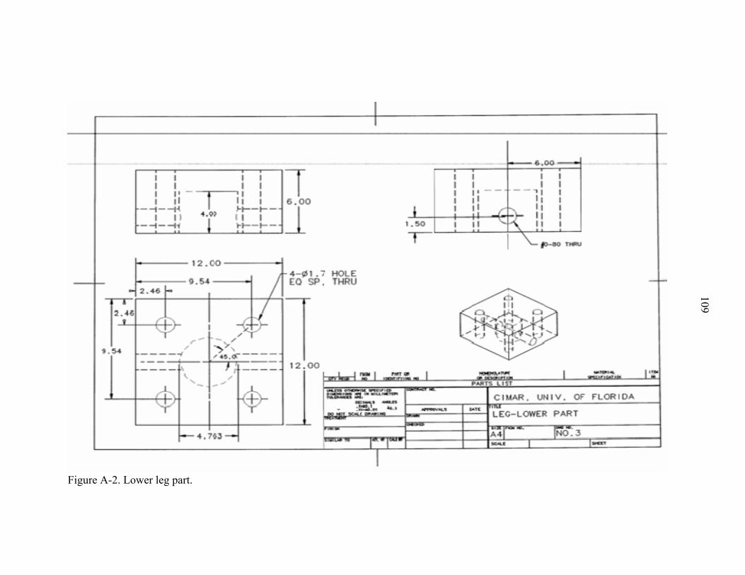
109

Figure A-2. Lower leg part.

110

Figure A-3. Upper leg part

111

Figure A-4. Leg

112

Figure A-5. Top plate.

113

Figure A-6. Base plate.

114

LIST OF REFERENCES

[Bal00] Ball, Robert Stawell, Treatise on the Theory of Screws, Cambridge University Press, Cambridge, UK, 1900.

[Cho02] Choi, K., and Jiang, S., “Spatial Stiffness Realization with Parallel Springs Using Geometric Parameters,” IEEE Trans. on Robotics and Automation, Vol. 18 (3), pp. 274-284, 2002.

[Cib99] Ciblak, N., and Lipkin, H., “Synthesis of Cartesian Stiffness for Robotic Applications,” in Proc. IEEE Int. Conf. Robotics and Automation, Detroit, MI, May 1999 pp. 2147–2151, 1999.

[Cra98] Crane, C.D., and Duffy, J., Kinematic Analysis of Robot manipulators, Cambridge University press, Cambridge, UK, 1998.

[Cra01] Crane, C.D., and Duffy, J.,Class Notes: Screw Theory and its Application to Spatial Robot Manipulators, MAE, University of Florida, Gainesville, FL, 2001.

[Dan95] Daniali H.R.M., and Zsombor-Murray P.J., “Singularity Analysis of a General Class of Planar Parallel Manipulators,” In IEEE Int. Conf. on Robotics and Automation, Nagoya , Japan, pp. 1547-1552, 1995.

[Das94] Dasgupta B., Reddy S., and Mruthyunjaya, T.S., “Synthesis of a Force-Torque Sensor Based on the Stewart Platform Mechanism,” Proc. National Convention of Industrial problems in Machines and Mechanisms, Bangalore, India, pp.14~23, 1994.

[Das98A] Dasgupta, B., and Mruthyunjaya, T.S., “A Newton-Euler Formulation for the Inverse Dynamics of the Stewart Platform Manipulator,” Mech. Mach. Theory, Vol. 33(8), pp. 1135-1152, 1998.

[Das98B] Dasgupta, B. and Mruthyunjaya, T.S. “Singularity-Free Path Planning for the Stewart Platform Manipulator,” Mechanism and Machine Theory, Vol. 33(6), pp.711-725, 1998.

[Das00]Dasgupta, B., and Mruthyunjaya, T.S., “The Stewart Platform Manipulator: A Review,” Mechanism and Machine Theory, Vol. 35, pp. 15~40, 2000.

[Dim65] Dimentberg, F.M., “The Screw Calculus and its Application in Mechanics,” Foreign Technology Division, Wright-patterson Air Force Base, Ohio. Document No. FTD-HT-23-1632-67, 1965.

115

[Duf96] Duffy, J, Statics and Kinematics with Applications to Robotics, Cambridge University press, Cambridge, UK, 1996.

[Dwa00]Dwarakanath, T., and Crane, C., “In-Parallel Passive Compliant Coupler for Robot Force Control,” Proceedings of the ASME Mechanisms Conference, Baltimore , MD, pp. 214-221, 2000.

[Fic86] Fichter, E.F., “A Stewart Platform-Based Manipulator: General Theory and Practical Construction,” Int. Journal of Robotics Research, Vol.5 Issue 2, pp. 157~181, 1986.

[Gai83] Gaillet, A and Reboulet, C., “An Isostatic Six Component Force and Torque Sensor,” Proc. 13th Int. Symposium on Industrial Robotics, Chicago, IL 1983.

[Gou62] Gough, V.E. and Whitehall, S.G., "Universal Tyre Test Machine," Proceedings of the FISITA Ninth Int. Technical Congress, London, UK, pp. 117-137, 1962.

[Gri89] Griffis, M., and Duffy, J., “A Forward Displacement Analysis of a Class of Stewart Platforms,” Journal of Robotic Systems, Vol. 6(6), pp. 703-720, 1989.

[Gri91A] Griffis, M., Kinestatic control: A Novel Theory for Simultaneously Regulating Force and Displacement, Ph.D. Dissertation, University of Florida, Gainesville, FL, 1991.

[Gri91B] Griffis, M., and Duffy, J., “Kinestatic Control: A Novel Theory for Simultaneously Regulating Force and Displacement,” Trans. ASME Journal of Mechanical Design, Vol. 113, No. 4, pp. 508-515, 1991.

[Gri93] Griffis, M., and Duffy, J., “Method and Apparatus for Controlling Geometrically Simple Parallel Mechanisms with Distinctive Connections,” United States Patent, Patent Number 5,179,525, Jan.12, 1993.

[Hua98] Huang, S., The Analysis and Synthesis of Spatial Compliance, PhD dissertation, Marquette Univ., Milwaukee, WI, 1998.

[Hun93] Hunt K.H. and Primrose E.J.F., “Assembly Configurations of Some In-Parallel Actuated Manipulators,” Mechanism and Machine Theory, Vol. 28(1), pp. 31-42, 1993.

[Hun98] Hunt, K.H., and McAree, P. R., “The Octahedral Manipulator: Geometry and Mobility,” The Int. Journal of Robotics Research, Vol. 17, No. 8, pp. 868-885, 1998.

[Inn93] Innocenti C. and Parenti C. V., “Closed-Form Direct Position Analysis of a 5-5 Parallel Mechanism,” ASME Journal of Mechanical Design, Vol. 115(3), pp. 515-521, 1993.

116

[Lee94] Lee, J., “An Investigation of A Quality Index for The Stability of In-Parallel Planar Platform Devices,” Master's Thesis, University of Florida, Gainesville, FL, 1996.

[Lee98] Lee, J., Duffy, J., and Hunt K., “A Practical Quality Index Based On the Octahedral Manipulator,” Int. Journal of Robotic Research, Vol.17 (10), pp. 1081-1090, 1998.

[Lee00] Lee, J., Investigation of Quality Indices of In-Parallel Platform Manipulators and Development of Web Based Analysis Tools, PhD Dissertation, University of Florida, Gainesville, FL, 2000.

[Lin 90] Lin, W., Duffy, J., and Griffis, M., "Forward Displacement Analysis of the 4-4 Stewart Platforms," in Proc. 21st Biennial Mech. Conf. ASME, Chicago, IL, Vol. DE-25, pp. 263-269, 1990.

[Lin94] Lin, W., Crane, C.D., and Duffy, J. “Closed Form Forward Displacement Analysis of the 4-5 In-Parallel Platforms,” ASME Journal of Mechanical Design, Vol. 116, pp. 47-53, 1994.

[Lon87] Loncaric, J., “Normal Forms of Stiffness and Compliance Matrices,”, IEEE Journal of Robotics and Automation, Vol. 3(6), pp. 567-572, 1987.

[Ma91] Ma O. and Angeles J, “Architecture Singularities of Platform Manipulator,” In. IEEE Int. Conf. on Robotics and Automation, Sacramento, CA, USA, pp. 1542-1547, 1991.

[Mer92] Merlet, J,, “Direct Kinematics and Assembly Models of Parallel Manipulators,” Int. Journal of Robotics Research, Vol. 11(2), pp.150-162, 1992.

[Mer00] Merlet, J., Parallel Robots, Kluwer Academic Publishers, Boston, MA, 2000.

[Ngu91] Nguyen C.C, and Antrazi, S.S. “Analysis and Implementation of a Stewart Platform-Based Force Sensor for Passive Compliant Robotic Assembly,” In IEEE Proc. of the Southeast Conf. 91, Williamsburg, VA, pp. 880-884, Williamsburg, 1991

[Pig98] Pigoski, T., Griffis, M., and Duffy, J., “Stiffness Mappings Employing Different Frames of Reference,” Mech. Mach. Theory Vol.33, No.6. pp. 825-838, 1998.

[Pol40] Pollard, W.L.G., "Spray Painting Machine," US Patent No. 2,213,108, August 26, 1940.

[Rag93] Raghavan, M., “The Stewart Platform of General Geometry has 40 Configurations,” Trans ASME J Mech. Trans. Automat Des Vol. 115, pp. 277~282, 1993.

117

[Rid02] Ridgeway, S., Research Proposal for Parallel Manipulator, MAE, University of Florida, Gainesville, FL, 2002.

[Rob00] Roberts, R.G., “Minimal Realization of an Arbitrary Spatial Stiffness Matrix with a Parallel Connection of Simple and Complex Springs,” IEEE Trans. on Robotics and Automation, Vol. 16(5), pp. 603-608, 2000.

[Rob02] Roberts, R.G.,” A Note on the Normal Form of a Spatial Stiffness Matrix,” IEEE Trans. on Robotics and Automation, Vol. 17(6), pp.968-972, 2001.

[Sel02] Selig, J.M. and Ding, X., “Structure of the Spatial Stiffness Matrix,” Int. Journal of Robotics and Automation, Vol. 17(1), pp.1-16, 2002.

[Ste65] Stewart, D., "A Platform with Six Degrees of Freedom," Proc of the IMechE, Vol. 180, Pt. 1, No. 15, pp. 371-385, 1965-66.

[Svi95] Svinin, M.M., and Uchiyama, M, “Optimal Geometric Structures of Force/Torque Sensors,” Int. journal of Robotics Research, Vol. 14(6), pp.560~573, 1995.

[Tsa99] Tsai, L.W., Robot Analysis, the Mechanics of Serial and Parallel Manipulators, John Wiley& Sons, New York, USA, 1999.

[Wam96] Wampler, C.W., “Forward Displacement Analysis of General Six-In-Parallel SPS (Stewart) Platform Manipulators Using soma coordinates,” Mechanism and Machine Theory, Vol. 31(3), pp.331-337,1996.

[Wen94] Wen F. and Liang C., “Displacement Analysis of the 6-6 Platform Mechanisms,” Mechanism and Machine Theory, Vol. 29(4), pp. 547-557, 1994.

[Zha04] Zhang, B, and Crane, C., “Special Singularity Analysis for a 6-DOF Parallel Platform,” 10th Int. Conference on Robotics & Remote Systems for Hazardous Environments, Gainesville, FL, USA, 2004.

118

BIOGRAPHICAL SKETCH

Bo Zhang was born in Xi’an, China, 1975. He received his Bachelor of Science

degree in mechanical engineering from XiDian University in his home town in 1997.

Then he went to Beijing to continue his study and received his Master of Science degree

in mechanical engineering from Tsinghua University in 2000. He found his strong

interest in robotics and joined the Department of Mechanical and Aerospace Engineering,

University of Florida, for his PhD degree in mechanical engineering. Since then, he has

continued his studies and worked as a research assistant with Dr. Carl D. Crane III at the

Center for Intelligent Machines and Robotics.

Documents

DESIGN AND IMPLEMENTATION OF A 6 DOF PARALLEL …