Design and Decoupling of Control System for a … 3/Issue 6/IJESIT201406_02.pdfISSN: 2319-5967 ISO 9001:2008 Certified International Journal of Engineering Science and Innovative Technology

ISSN: 2319-5967

ISO 9001:2008 Certified International Journal of Engineering Science and Innovative Technology (IJESIT)

Volume 3, Issue 6, November 2014

9

Design and Decoupling of Control System for

a Continuous Stirred Tank Reactor (CSTR) Georgeous, N.B

*1 and Gasmalseed, G.A, Abdalla, B.K

(1-2) University of Science and Technology, Sudan Department of Chemical Engineering.

Abstract: To apply the methods of stability analysis and tuning, it is necessary first to develop a control strategy for

possible noninteracting and interacting loops. Then the transfer functions were identified by mathematical modeling and

the overall gains were cited from the literature. Pairing of the loops were undertaken and the interact in loops were

coupled according to the RGA (Relative Gain Array), thus the loops with minimal interaction were selected and put in

block diagrams. The characteristic equations were obtained for both closed and open loops. An exothermic reaction in a

continuous stirred tank reactor (CSTR) was selected as a case study. The loops were subjected to tuning, stability and

offset investigation. Summary of the adjustable parameters, offsets and response behavior were tabulated for comparison

between the methods. It is clear that all the methods are in agreement, but the Bode criteria showed a superior

consistency over other methods. It is recommended that the method of Bode has to be preferentially selected for tuning

and stability analysis.

Index Terms: Methods of tuning, Stability, Transfer function identification, Offset investigation.

I. INTRODUCTION

A control system is composed of interacting loops and that the number of feasible alternative configurations

needed to be configured are very large. It must be recognized that for a process with n controlled variables and n

manipulated variables there are n different ways to form control the loops [1]

. The question is which one to

selected? The answer is to consider the interaction between the loops for all n loops and then the RGA is

applied to select a loop when the interaction is minimal. The RGA provides such a methodology by pairing the

input and output that give minimum interaction when together coupled, RGA was first proposed by Bristol and

today it is a very popular tool for selection of control loops giving minimal interaction [1].The methods of

pairings and the RGA were applied to an exothermic reaction in a jacketed CSTR, the process is a 2 2

controlled and manipulated variables. The method of stability and tuning were applied using Routh-Hurwitz,

direct substitution, root-Locus, and Bode and Nyquist criteria.

II. OBJECTIVES

1- To select the loops with minimal interaction in CSTR.

2- To study the dynamics of a CSTR.

3- To investigate the methods of tuning and stability analysis.

4- To compare the accuracy of these methods with respect to stability, adjustable parameters and offset.

III. LITERATURE REVIEW

Multiple input, multiple output (MIMO) systems describe processes with more than one input and more than

one output which require multiple control loops. Examples of MIMO systems include heat exchangers, chemical

reactors, and distillation columns. These systems can be complicated through loop interactions that result in

variables with unexpected effects. Decoupling the variables of that system will improve the control of that

process [2].

An example of a MIMO system is a jacketed CSTR in which the formation of the product is dependent upon the

reactor temperature and feed flow rate. The process is controlled by two loops, a composition control loop and a

temperature control loop. Changes to the feed rate are used to control the product composition and changes to

the reactor temperature are made by increasing or decreasing the temperature of the jacket. However, changes

made to the feed would change the reaction mass, and hence the temperature, and changes made to temperature

would change the reaction rate, and hence influence the composition. This is an example of loop interactions.

Loop interactions need to be avoided because changes in one loop might cause destabilizing changes in another

loop [2]. To avoid loop interactions, MIMO systems can be decoupled into separate loops known as single

ISSN: 2319-5967



10

input, single output (SISO) systems. Decoupling may be done using several different techniques, including

restructuring the pairing of variables, minimizing interactions by detuning conflicting control loops, opening

loops and putting them in manual control, and using linear combinations of manipulated and/or controlled

variables. If the system can’t be decoupled, then other methods such as neural networks or model predictive

control should be used to characterize the system [2,3,4].

There are two ways to see if a system can be decoupled. One way is with mathematical models and the other

way is a more intuitive educated guessing method. Mathematical methods for simplifying MIMO control

schemes include the relative gain array (RGA)[2]

. The RGA provides a quantitative approach to the analysis of

the interactions between the controls and the output, and thus provides a method of pairing manipulated and

controlled variables to generate a control scheme. The RGA is a normalized form of the gain matrix that

describes the impact of each control variable on the output, relative to each control variable's impact on other

variables. The process interaction of open-loop and closed-loop control systems are measured for all possible

input-output variable pairings [5]. A ratio of this open-loop gain to this closed-loop gain is determined and the

results are displayed in a matrix. The array will be a matrix with one column for each input variable and one row

for each output variable in the MIMO system[5]

. The best pairing is discovered by taking the maximum value of

RGA Matrix for each row.

A digital computer can be used to control simultaneously several outputs, the control program is composed of

several subprograms, each one used to control a different loop. Furthermore, the control program should be able

to coordinate the execution of the various subprograms so that each loop and all together function properly [6].

Although a controller may be stable when implemented as an analog controller, it could be unstable when

implemented as a digital controller due to a large sampling interval. During sampling the aliasing modifies the

cutoff parameters. Thus the sample rate characterizes the transient response and stability of the compensated

system, and must update the values at the controller input often enough so as to not cause instability. When

substituting the frequency into the z operator, regular stability criteria still apply to discrete control systems.

Nyquist criteria apply to z-domain transfer functions as well as being general for complex valued functions.

Bode stability criteria apply similarly. Jury criterion determines the discrete system stability about its

characteristic polynomial [6].

The system stability can be tested by considering its response to a finite input signal. This means the analysis of

system dynamics in the actual time domain which is usually cumbersome and time consuming. Several methods

have been developed to deduce the system stability from its characteristic equation. They are short-cut methods

for providing information without finding out the actual response of the system. They give information from the

s-domain without going back to the actual time-domain. All these methods are based on the criterion that a

sufficient condition for stability of a control loop is to have a characteristic equation with only negative real

roots and or complex roots with negative real parts. The short-cut methods for assessment of the stability of a

system include the direct method, the Routh–Hurwitz stability criterion and graphical methods of investigating

the behavior of the roots of the characteristic equation, i.e. Root Locus method and Nyquist stability criterion.

Bode plots are common graphical method. It depends only upon the open loop transfer function (OLTF). The

OLTF relates the feedback or measured variable to the set point, when the feedback loop is disconnected from

the comparator when the loop is broken or opened.

IV. RESULTS AND DISCUSSION

Interaction, coupling and control of CSTR

Consider a process with two controlled outputs and two manipulated inputs (Figure 1.). The transfer functions

are:

1.GC1(s)= KC1, ….(1)

2.GC2(s)= KC2, ….(2)

3.Gf1(s)= , ….(3)

http://controls.engin.umich.edu/wiki/index.php/NN

http://en.wikipedia.org/wiki/Nyquist_stability_criterion

http://en.wikipedia.org/wiki/Jury_stability_criterion

ISSN: 2319-5967



11

4.Gf2(s)= , ….(4)

5.Gm1(s)= , ….(5)

6.Gm2(s)= , ….(6)

7. H11(s)= , ….(7)

8.H12(s)= , ….(8)

9.H21(s)= , ….(9)

10.H22(s)= . ….(10)

Loop 1

-

,sp + + +

,sp + - + +

Loop 2

Fig 1. Block diagram of CSTR with two controlled outputs and two manipulative variables.

The Routh–Hurwitz stability criterion is used for determination the stability of a system, the characteristic

equation of closed loop is used. Also Bode plots, root-Locus method and Nyquist stability criterion are used for

determination the stability of a system, the OLTF is used. The amplitude ratio (AR) is used to get the ultimate

gain(KU) and Ziegler-Nichols tuning is brought to edge of stability under proportional control and it is used for

tuning the adjustable parameters, which are substituted in overall gains for study the response.

Loop 1 is closed and loop 2 is open, the transfer function is:

….(11)

….(12)

GC1(s)

H22

Gm2(s)

GC2(s) Gf2(s)

H21

H12

H11

Gm1(s)

Gf1(s)

ISSN: 2319-5967



12

….(13)

The characteristic equation of closed loop is: 0.15 s4 +1.45s

3 + 3.85 s

2 +3.6 s + (1+ KC1) = 0 ….(14)

Putting the characteristic equation in Routh Array:

Table 1: Routh-Hurwitz Array

For the system to be critically stable: (3.183-0.417 KC1) = 0, KC1= KU1 = 7.633, The system become stable for all

values of KC1 KU1 7.633. The auxiliary equation is1.45s3

+3.6 s = 0, s= iω; ωco = 1.5757 rad / sec; Pu =

= = 3.99 sec.

Tuning:

Applying Ziegler- Nichols method ( Z-N method):

Table 2: Z-N adjustable parameters for loop 1

Controller mode KC1 τI ( sec) τD ( sec)

P 3.8165 - -

PI 3.4349 3.325 -

PID 4.5798 1.995 0.4988

Substituting the value of KC1 = 3.8165 of proportional controller (P- action) in characteristic equation,0.15 s4

+1.45s3

+ 3.85 s2 +3.6 s + 4.8165= 0 and in first column of Routh array. All elements of the first column were

positive and there is no change of sign, therefore the system is stable.

Response:

Substituting the value of KC1 in the transfer function of loop1 (G(s)) and introducing an impulse forcing function:

Impulse Response

Time (seconds)

Ampli

tude

0 5 10 15 20 25 30-0.5

0

0.5

1

System: sys

Peak amplitude: 0.849

At time (seconds): 1.12

System: sys

Settling time (seconds): 16.9

Fig 2. Impulse response when loop1 is closed.

S4 0.15 3.85 (1+ KC1) 0

S3 1.45 3.6 0 0

S2 3.4776 (1+ KC1) 0 0

S1 (3.183-0.417 KC1) 0 0 0

S0 (1+ KC1) 0 0 0

ISSN: 2319-5967



13

Bode analysis and tuning:

Open loop transfer function (OLTF) of loop 1is:

….(15)

Fig 3. Bode diagram when loop1 is open

From Bode diagram, ωco =1.58 rad /sec and the amplitude ratio (AR)= 1, Pu = = 3.98 sec, the amplitude

ratio (AR) is used to get KC1.

1= ….(16)

Substituting the value of ωco = 1.58 rad / sec in the equation to get KC1,KC1= KU1= 7.9962

Response:

For Kc1 = 3.9981

Impulse Response

Time (seconds)

Ampl

itude

0 5 10 15 20 25 30-0.6

-0.4

-0.2

0

0.2

0.4

0.6

0.8

1

System: sys



System: sys


Fig 4.Impulse response when loop1 is closed.

-250

-200

-150

-100

-50

0

Magn

itude

(dB)

Bode Diagram

Frequency (rad/s)

10-2

10-1

100

101

102

103

-360

-270

-180

-90

0

System: sys

Frequency (rad/s): 1.58

Phase (deg): -180

Phas

e (de

g)

ISSN: 2319-5967



14

Root Locus:

Root Locus

Real Axis (seconds-1)

Imag

inary

Axis

(sec

onds

-1)

-20 -15 -10 -5 0 5 10 15-15

-10

-5

0

5

10

15

System: sys

Gain: 7.52

Pole: -0.00429 + 1.57i

Damping: 0.00273

Overshoot (%): 99.1


Fig 5.Root-Locus diagram when loop1 is open

From root-Locus diagram, ωco = 1.57 rad / sec and the amplitude ratio (AR) = 1, KC1= KU1= 7.8939

Response:

For Kc1 = 3.9469

Impulse Response

Time (seconds)

Ampli

tude

0 5 10 15 20 25 30-0.6

-0.4

-0.2

0

0.2

0.4

0.6

0.8

1

System: sys



System: sys


Fig 6. Impulse response when loop1 is closed.

Nyquist stability criterion:

Nyquist Diagram

Real Axis

Imag

inary

Axis

-1 -0.5 0 0.5 1 1.5-0.8

-0.6

-0.4

-0.2

0

0.2

0.4

0.6

0.8

System: sys

Real: -0.132

Imag: 0.00326

Frequency (rad/s): -1.58

Fig 7. Nyquist diagram when loop1 is open

From Nyquist diagram, ωco = 1.58 rad / sec.The characteristic equation of closed loop is:

0.15 s4 +1.45s

3 + 3.85 s

2 +3.6 s + (1+ KC1) = 0 ….(14)

0.15 ω 4 -1.45 iω

3 - 3.85 ω

2 +3.6 iω + (1+ KC1) = 0 ….(17)

ISSN: 2319-5967



15

0.15 ω 4 - 3.85 ω

2 + (1+ KC1) = 0 ….(18)

Substituting the value of ωco = 1.58 rad / sec to get KC1, KC1= KU1 = 7.6763

Response: For Kc1 = 3.8382

Impulse Response

Time (seconds)

Am

plitu

de

0 5 10 15 20 25 30-0.5

0

0.5

1

System: sys



System: sys


Fig 8. Impulse response when loop1 is closed

Table 3: Comparison between the methods for continuous stirred tank reactor ( CSTR ) of loop1

Method KU PU

(sec)

KC

Routh-

Durwitz

7.633 3.99 3.8165 -0.2076

Bode 7.9962 3.98 3.9981 -0.2001

Root-Locus 7.8939 4.00 3.9469 -0.2021

Nyquist 7.6763 3.98 3.8382 -0.2067

Table 4: Comparison between the methods for continuous stirred tank reactor ( CSTR ) of loop1

Method Overshoot Rise

time(sec)

Settling

time(sec)

Routh-Durwitz 0.849 1.12 16.9

Bode 0.886 1.11 18.9

Root-Locus 0.875 1.11 18.8

Nyquist 0.854 1.12 16.9

Loop 2 is closed and loop 1 is open, the transfer function is:

….(19)

The characteristic equation is: 0.4 S5 + 2.4 s

4 +5.7s

3 + 7.1 s

2 +4.4 s + (1+ 2KC2) = 0 ….(20)

The preceding procedure is applied.

Table 5: Routh-Hurwitz Array

S5 0.4 5.7 4.4 0

S4 2.4 7.1 (1+ 2KC2) 0

S3 4.5167 (4.23-0.33KC2) 0 0

S2 (4.85+0.18 KC2) (1+ 2KC2) 0 0

ISSN: 2319-5967



16

S1

( ) 0 0 0

S0 (1+2 KC2) 0 0 0

KU2 = 1.6029, ωco= 0.906 rad / sec, Pu = = 6.94 sec, KC2 = 0.8015.


Impulse Response

Time (seconds)

Ampli

tude

0 5 10 15 20 25 30 35-0.2

-0.1

0

0.1

0.2

0.3

0.4

0.5

System: sys



System: sys



Bode analysis and tuning:

Open loop transfer function (OLTF) of loop 2is:

….(21)

-200

-150

-100

-50

0

50

Mag

nitu

de (

dB)

Bode Diagram

Frequency (rad/s)

10-2

10-1

100

101

102

-450

-360

-270

-180

-90

0System: sys


Phase (deg): -180

Pha

se (

deg)

Fig 10. Bode diagram when loop2 is open

ISSN: 2319-5967



17

From Bode diagram, ωco = 0.906 rad / sec, Pu = = 6.9379 sec, and the amplitude ratio (AR) = 1=

….(22)

KC2= KU2= 1.6054.

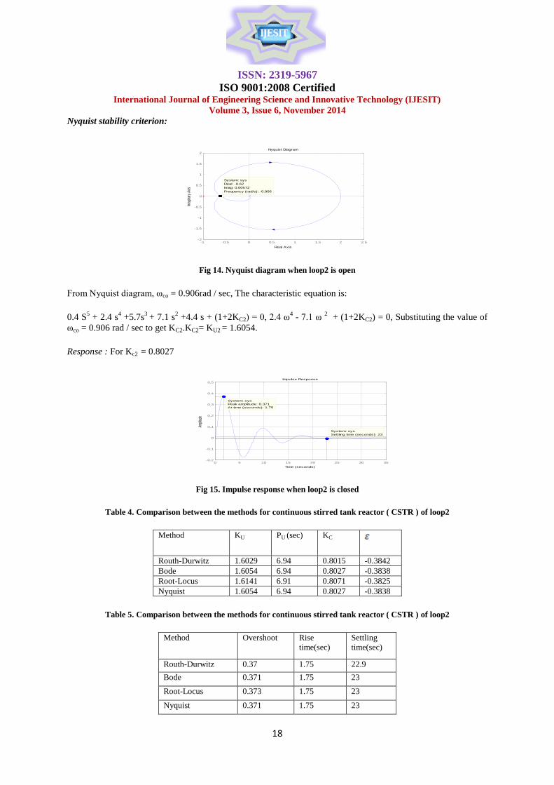
Response : For Kc2 = 0.8027

Impulse Response

Time (seconds)

Ampl

itude

0 5 10 15 20 25 30 35-0.2

-0.1

0

0.1

0.2

0.3

0.4

0.5

System: sys

Settling time (seconds): 23

System: sys




Root Locus:

Root Locus

Real Axis (seconds-1)

Imag

inary

Axis

(sec

onds

-1)

-8 -6 -4 -2 0 2 4-6

-4

-2

0

2

4

6

System: sys

Gain: 1.64

Pole: 0.00626 + 0.909i

Damping: -0.00689

Overshoot (%): 102


Fig 12. Root-Locus diagram when loop2 is open

From root-Locus diagram, ωco = 0.909 rad / sec and the amplitude ratio (AR) = 1, KC2= KU2= 1.6141.


Impulse Response

Time (seconds)

Am

plitu

de

0 5 10 15 20 25 30 35-0.2

-0.1

0

0.1

0.2

0.3

0.4

0.5

System: sys


System: sys




ISSN: 2319-5967



18

Nyquist stability criterion:

-1 -0.5 0 0.5 1 1.5 2 2.5-2

-1.5

-1

-0.5

0

0.5

1

1.5

2

System: sys

Real: -0.62

Imag: 0.00572

Frequency (rad/s): -0.906

Nyquist Diagram

Real Axis

Imag

inar

y Ax

is

Fig 14. Nyquist diagram when loop2 is open

From Nyquist diagram, ωco = 0.906rad / sec, The characteristic equation is:

0.4 S5 + 2.4 s

4 +5.7s

3 + 7.1 s

2 +4.4 s + (1+2KC2) = 0, 2.4 ω

4 - 7.1 ω

2 + (1+2KC2) = 0, Substituting the value of

ωco = 0.906 rad / sec to get KC2.KC2= KU2 = 1.6054.

Response : For Kc2 = 0.8027

Impulse Response

Time (seconds)

Ampli

tude

0 5 10 15 20 25 30 35-0.2

-0.1

0

0.1

0.2

0.3

0.4

0.5

System: sys


System: sys




Table 4. Comparison between the methods for continuous stirred tank reactor ( CSTR ) of loop2

Method KU PU (sec) KC

Routh-Durwitz 1.6029 6.94 0.8015 -0.3842

Bode 1.6054 6.94 0.8027 -0.3838

Root-Locus 1.6141 6.91 0.8071 -0.3825

Nyquist 1.6054 6.94 0.8027 -0.3838

Table 5. Comparison between the methods for continuous stirred tank reactor ( CSTR ) of loop2

Method Overshoot Rise

time(sec)

Settling

time(sec)

Routh-Durwitz 0.37 1.75 22.9

Bode 0.371 1.75 23

Root-Locus 0.373 1.75 23

Nyquist 0.371 1.75 23

ISSN: 2319-5967



19

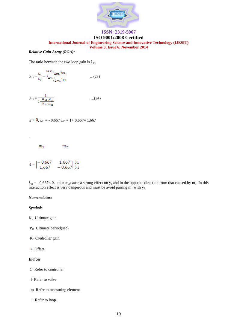
Relative Gain Array (RGA):

The ratio between the two loop gain is λ11,

λ11 = = ….(23)

λ11 = ….(24)

s , λ11 = - 0.667, λ12 = 1+ 0.667= 1.667

.

=

λ11 = - 0.667< 0, , then m2 cause a strong effect on y1 and in the opposite direction from that caused by m1. In this

interaction effect is very dangerous and must be avoid pairing m1 with y2.

Nomenclature

Symbols

KU Ultimate gain

PU Ultimate period(sec)

KC Controller gain

Offset

Indices

C Refer to controller

f Refer to valve

m Refer to measuring element

1 Refer to loop1

ISSN: 2319-5967



20

2 Refer to loop2

V. CONCLUSION

It is clear that all the methods are in agreement, but the Bode criterion has to be preferentially selected for tuning

and stability analysis. For CSTR, λ11 = - 0.667, then m2 cause a strong effect on y1 and in the opposite direction

from that caused by m1. In this interaction effect is very dangerous.

ACKNOWLEDGMENT

The authors wish to thank the Collage of Higher Studies and Research of Karary University for their help and

for giving us opportunity for carrying out research in partial fulfillment for Ph.D in Chemical Engineering.

REFERENCES [1] Stephanopoulos, G. (2005), Chemical Process Control, Prentice-Hall, India.

[2] Tham, M.T. (1999). "Multivariable Control: An Introduction to Decoupling Control". Department of Chemical and

Process Engineering, University of Newcastle upon Tyne.

[3] McMillan, Gregory K. (1983) Tuning and Control Loop Performance. Instrument Society of America. ISBN 0-87664-

694-1.

[4] Lee, Jay H., Choi, Jin Hoon, and Lee, Kwang Soon. (1997). "3.2 Interaction and I/O Pairing". Chemical Engineering

Research Information Center.

[5] Berber, Ridvan. (1994).Methods of Model Based Process Control, Kluwer Academic Publishers.

[6] FRANKLIN, G.F.; POWELL, J.D. (1981). Digital control of dynamical systems. USA, California: Addison-Wesley.

ISBN 0-201-82054-4.

Documents

Design and Decoupling of Control System for a … 3/Issue 6/IJESIT201406_02.pdfISSN: 2319-5967 ISO 9001:2008 Certified International Journal of Engineering Science and Innovative Technology