ISSN: 2319-5967 ISO 9001:2008 Certified International ... 3/Issue 5/IJESIT201405_10.pdf · tedious .In the sour water stripping column in ... of the loops and then design ... as condensates

ISSN: 2319-5967

ISO 9001:2008 Certified International Journal of Engineering Science and Innovative Technology (IJESIT)

Volume 3, Issue 5, September 2014

95

Interaction, Parings, and decoupling of sour

water stripping unit S. O .AlhagAli, G.A.Gasmelseed, I.H.Elamin

Department of Chemical Engineering, Faculty of Engineering, University of Science and Technology

Telephone:+249912475667, +249919634134, +249912306041

Abstract: Interactions among control loops in distillation and stripping columns are quite common, and sometimes

becomes very serious. It disturbs the stability of the control system and makes the tuning process rather difficult and

tedious .In the sour water stripping column in Khartoum refinery , interaction exists between the feed rate (F) and top

plate temperature (T),as well as between the feed rate (F) and the level (L) in the reflux drum. Simultaneously interaction

exists between the reflux ratio(R) and the top temperature (T)and also exists between the reflux ratio ( R) and level (L)in

the reflux drum .These interacting loops need to be decoupled by connecting loops with minimal interaction .The

procedure is to develop a control strategy , identify the transfer functions of the elements of the loops and then design

proper pairings according to the relative gain array (RGA)method. The RGA determines loops with minimal interaction

and helps in decoupling ,however ,RGA shows loops that have comparatively minimum interaction, but does not

eliminate the interaction ,and some time the interaction needs installation of decouples .In this study a control system was

designed, loops with minimum interaction were connected , tuned , and their stability and offset investigation were

carried out using different techniques including Routh-Hurwitz , Root Locus , Bode Plot, and Nyquist .A complete

control system of the sour water treatment plant is designed with decouplers , the same is interfaced to digital, Control

system (PLC).

Index terms: Pairing, decoupling, sour water, stripping, digital control.

I. INTRODUCTION

A. Sour Water Stripping Unit

Sour water is any water from a refinery that contains hydrogen sulphide. In addition, sour water may contain

ammonia, light hydrocarbons. Sour Water comes from: Atmospheric Crude distillation, catalytic cracking

reforming and Delayed Coking Unit, distillation column produces sour water as condensates from steam that

used in injection and stripping. Another major source of sour water is hydro-treater wash water. [1]

Brief introduction of the sour water stripping unit

Sour water stripping unit of Khartoum Refinery is a single-column low- pressure stripping process, The

construction started from the year 2009, and was commissioned in May 2010. The feedstock for the unit is the

sour water coming from Residual Fluid Catalytic cracking （RFCC）, Delayed Coking Unit（DCU）, Coker

gasoline/diesel Hydro-treating （GDHT）as well as Diesel Hydro fining Unit （DHT）etc. Design processing

capacity of the unit is 1.0 million t/year. The unit consists of sour water pretreatment system, sour water

stripping system（SWS）, acid gas Incinerator system（AGI）, and waste gas sweetening facility

system（WGS）and condensate water recovery system （CWR）. [1].

II. MATERIALS AND METHODS

A control strategy was developed, interacting loops were paired, transfer functions have been identified and

loops with minimal interactions were coupled together .The coupled loops had to be analyzed for stability and

tuning. By Routh -Hurwitz, Root Locus, Direct substitution, and Bode methods.

A. Routh-Hurwitz criterion for stability

The Routh test is a purely algebraic method for determining how many roots of the characteristic equation have

positive real parts; from which it can be seen whether the system is stable, for if there are no roots with positive

real parts, the system is stable or unstable. [2]

B. Root locus

The root loci are merely the plots in the complex plane of the roots of the characteristic equation as the gain

varied from zero to infinity. [3].

ISSN: 2319-5967



96

C. Direct substitution method

This method is a simple way to find the values of parameters in the characteristic equation that put the system

just at the limit of stability. This means that the roots are pure imaginary numbers (zeros real parts) at the brink

of instability. [4].

D. Roots solving method

This method is based on determining the roots of the characteristic equation. The application of this method was

limited by the mathematical difficulty in evaluating roots of high order polynomials, where a computer software

has to be used.

E. Frequency Response methods

Frequency response concepts and techniques play an important role on stability analysis. A much more practical

approach now utilizes spreadsheets or control-oriented software such as MATLAB to simplify calculations and

generates Bode and Nyquist plots.

- Bode plot: TheBode diagram consists of a log-log plot of the amplitude ratio(AR) versus

frequency ω and a semilog plot of versus .These plots are particularly useful for rapid analysis of

the response characteristics and stability of closed-loop systems.

- Nyquist plot: A Nyquist plot also called a polar plot inS-plane of the amplitude ratio versus

phase angle as the frequency is varied from zero to infinity.

F. Relative stability

To know that the system is stable is not generally sufficient for the requirements of control system design. There

is a need for stability analysis to determine how close the system is closed to instability and how much is the

margin when disturbances are present and when the gain is adjusted. [5] Relative Stability is represented by real

part of each root. The more negative stability of each root is clearly necessary. This method is superseded by the

root –solving method where exact values of the roots may be determined. [6]

G. Interacting of Control loops

For the design of control system for processes with multiple inputs and multiple outputs (MIMO) two

characteristics must be clear:

1-A control system is composed of several interacting control loops.

2-The number of feasible alternative configurations of control loops is very large and equal N! ,Where N is the

number of controlled and manipulated variables[3].

III. OBJECTIVES

1-To develop a control strategy of sour water striping unit in Khartoum refinery

2- To identify the transfer functions

3-To investigate the tuning and stability analysis.

4- To present response simulation at the values of the tuned adjustable parameters.

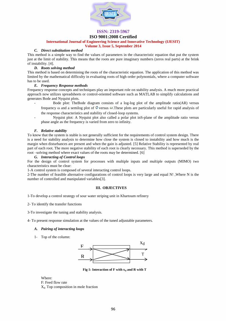
A. Pairing of interacting loops

1- Top of the column:

Fig 1: Interaction of F with xd and R with T

Where:

F: Feed flow rate

Xd: Top composition in mole fraction

F

R

xd

T

http://www.roymech.co.uk/Related/Control/Frequency_Response.html

ISSN: 2319-5967



97

R: Reflux ratio

T: Top temperature

Feed rate affects the composition of the product and top temperature ,loop1.

The reflux ratio affects the temperature at the top and the composition of the product, loop2.

2- Base of the column:

Fig 2: Interaction of B with Land T. and m.s with T

Where:

B: Bottom flow rate

L: Base level

ms: Steam Flow rate

T: Bottom temperature

The bottom rate affects the level at the base and temperature at the lower plates, loop3. The steam rate affects

the temperature at the lower plates and the level at the base of the column

B. Identification of transfer functions of control loops

From the literature [4] the following transfer functions are obtained:

Loop1:

GP = ………………………………………………………..…..….…(1)

Gm = 1.0

GV = ………………………………………………….…...……….(2)

GC = KC

Loop2:

GP = …………………………….…………………………..………….……(3)

Gm = ……………………………………………………..….....………….(4)

GV = ……………………………………………..…....………..…(5)

GC = KC

Loop3:

GP = ………………………………………………………....………….…(6)

Gm = ………………………………………………………...…...…….….(7)

Bottom rate, B

Steam rate ,m,s

L

T

ISSN: 2319-5967



98

GV = ………………………………..……………………………..….….(8)

GC = KC

Loop4:

GP = ……………………………………..…………………………….……(9)

Gm = …………………………………………………………….…..…….(10)

GV = …………………………………………………………..…….....…(11)

GC = KC

C. Interaction and decoupling of interacting loops (loop1andloop2)

Loop1and loop2:

=

Figure 3:Block diagram of interacting systems of loop1and loop2

+ +

+

=

KC

F xd

-

1.0

+

KC

R

T

-

+

M1

M2

+ -

ISSN: 2319-5967



99

From figure (3): the following relations were obtained:

H11 = …………………….…...…...…(12)

H21 = ………………………..……....……(13)

H12 = ………………………………….…….(14)

H22 = ……………..………………….……..(15)

Where :

H11 ,H21,H12 , H22 are the four transfer functions relating the two outputs(xd,T)to the two inputs(F,R), the

interaction indicates are calculated as follows:

y-11 = ………………….………....…(16)

y-1 = m

-1 + m

-2 …....………….…..…(17)

y-2 = m

-1 + m

-2 ...………………………..(18)

k11=[ ] ……………………….………...….(19)

y-11 = = 3 ………………………….….…..(20)

m-1 m

-2

Λ = 3 -2 y-1

-2 3 y-2

The coupling would be as follows:

y-1coupling with m

-1

and y-2 was coupled with m

-2

The block diagrams of loops with minimal interactions according to the RGA are as shown in the following

figure:

ISSN: 2319-5967



100

Fig 4: Block diagram of loops with minimal interaction

D. Tuning and stability analysis

The Overall transfer function = …………………………..…………………….….(21)

Where : πf = multiplication of the forward transfer functions

πl = multiplication of the loop transfer functions

The open loop transfer function of the loop 1:

OLTF = ………………………………..….…..……....…(22)

1+πl=1+ ……….……………………..…….……..….……(23)

1+πl= ………………………………...…..……..…(24)

The characteristic equation is 1+πl=0

The Characteristic equation of loop1 is:

=0 …………………….....…….…(25)

ISSN: 2319-5967



101

0.5S4 + 3.75S

3+ 6.75S

2 +4.5S+1+0.35KC = 0 …………….……………………….…..(26)

To tune loop 1 using Z-N method the value of ultimate gain Ku and ultimate period Pu were determined using

Routh Hurwitz, Root locus and bode criteria.

Tuning of loop 1

Routh- Hurwitz method

Routh Array:

S4

0.5 6.75 1+3.5KC

S3

3.75 4.5 0

S2

6.15 0

S 27.5-(3.75+13.125Kc) 0 0

S0

3.75+13.125kc 0 0

27.5-(3.75+13.125Kc) = 0 ………………….……………………………………….…….(27)

23.75-13.125Kc =0 ………………………………………………………….…….……..(28)

23.75 = 13.125Kc ………………………………………………………………………..(29)

Kc = 1.81 , Kc = Ku ……...………………………………………………………………(30)

Ku = 1.81 ….……………………………………………………………………………..(31)

Pu = ……………………………………………………………………..………….(32)

To determine ωco direct substitution method was used:

Taking the auxiliary equation:

Set s= i

Where = frequency in rad/sec

6.75S2 + 1+ 3.5 Kc =0 ……………………………………………………….……………(33)

6.75S2 + (1+3.5*1.81) =0 …………………………………………….……..……………(34)

6.75( i )2 = -(1+3.5*1.81) ……………………………………………………………….(35)

-6.75ω2 = - 7.335 …………..………………………………………….…………………(36)

ω2 = 1.09 then ω = 1.044 and ω = ωco ……………………………………... …...….(37)

ωco = 1.044 rad/sec ……………………………………………………………………(38)

ISSN: 2319-5967



102

Pu = then Pu = = 6.02 ………………………………………………….…......(39)

Table (1): Using Ziegler – Nichols’ method to specify the tuning parameters of loop 1

Type of

Controller

Kc

I ,sec

τD ,sec

P 0.91 - -

PI 0.82 5.02 -

PID 1.086 3.01 0.753

Response of the system:

G(s) = …………………….……………………..……(40)

G(s) = ……….…………………….………………(41)

G(s) = …………...………………….……………….….(42)

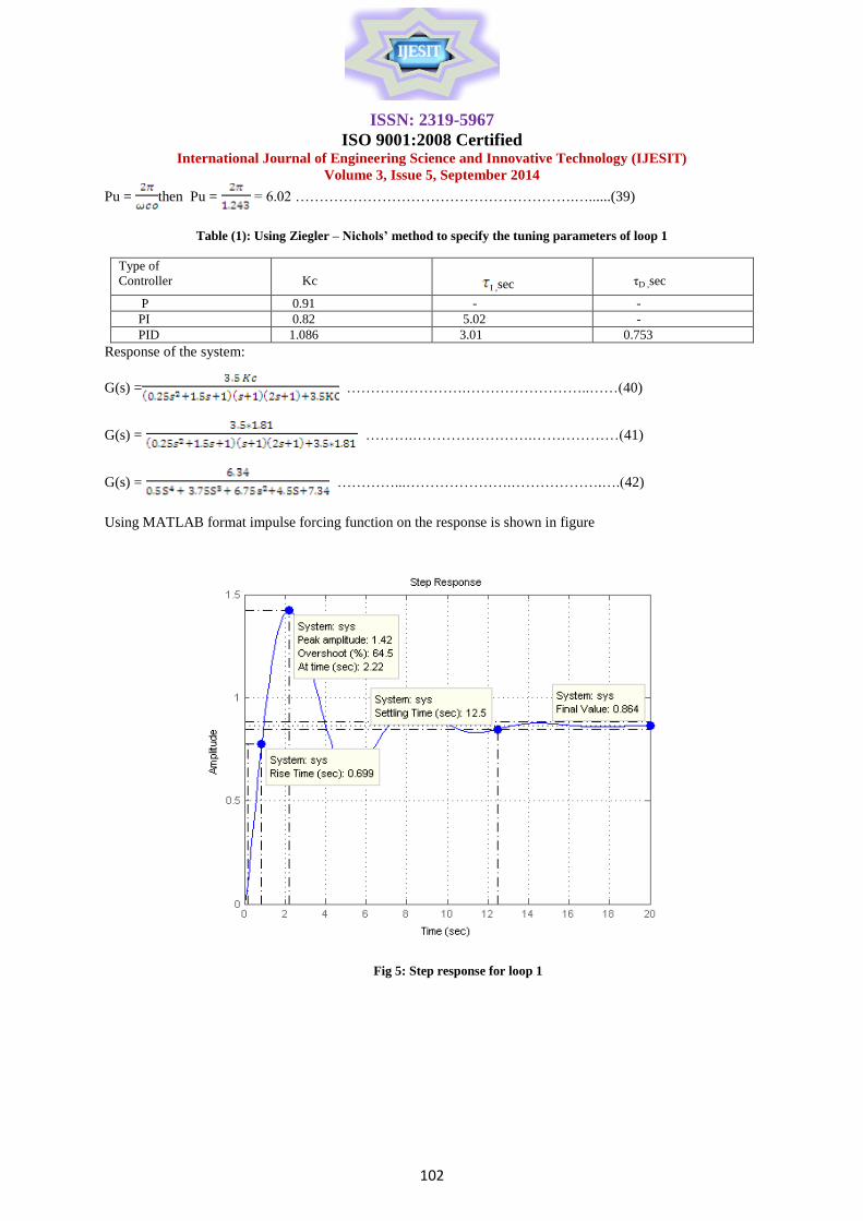
Using MATLAB format impulse forcing function on the response is shown in figure

Fig 5: Step response for loop 1

ISSN: 2319-5967



103

Table (2) Characteristic of Step response for loop 1

Characteristic Value

Peak amplitude at time (sec)

1.42

Over shoot (%)

64.5

Settling Time (sec)

12.5

Rise Time (sec)

0.699

Final Value

0.864

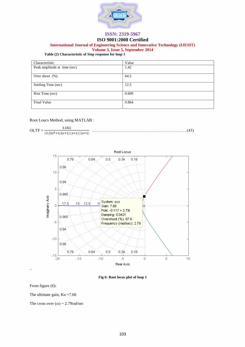
Root Loucs Method, using MATLAB :

OLTF = ……………………………………………………………(43)

..

Fig 6: Root locus plot of loop 1

From figure (6):

The ultimate gain, Ku =7.66

The cross over (ω) = 2.79rad/sec

ISSN: 2319-5967



104

Pu = = =2.25 sec ………………………………………………………….…………(44)

Table (3): Values of the adjustable parameters using Zeigler- Nichol’s

Type of

controller

KC

τI,sec

τD,sec

P 3.38 - -

PI 3.45 1.88 -

PID 4.596 1.125 0.283

The Bode plot method, using MATLAB

1+OLTF=0 …………………………………………………………………………………..(45)

1+ = 0 …………………………………………………...……...(46)

Fig 7: Bode plot of loop 1

From figure (7):

Frequency = 2.9rad/sec

Phase=-180°

AR= ……………………………………………………………(47)

At the cross-over frequency, AR=1

ISSN: 2319-5967



105

* * ) * ) =Kc

Kc=49.25

Pu= ……………………………………………….…………………………………….(48)

Pu =2 ………………………………………………………………………………..(49)

Pu= 2.16

Table (4): Tuning using Zeigler-Nichol’s

Type of

Controller

Kc

τI(sec)

τD(sec)

P 24.6 - -

PI 22.2 1.8 -

PID 29.6 1.08 0.27

Offset investigation for loop1:

G(s) = ……….….…………………………….….…..(50)

Kc=1.8

G(s) = …………….…………………………………..(51)

Taking a unit step:

r(t) =1

R(s) = …………..……………………………….……………………...……..…….…(52)

Є = C∞ - Cid ………………………………………..………………………………..…..(53)

C∞ = ………………..……………..……………………………..…(54)

………………………...……..….(55)

Cid = 1

Є = 0.864 – 1= -0.136

The same procedure was repeated for loops2, with results shown in figure: (8,910) respectively

ISSN: 2319-5967



106

Fig 8: Step response for loop 2

Table (6): Characteristic of Step response for loop 2

Characteristic value

Peak amplitude at time (sec)

2.42

Over shoot (%)

166

Settling Time (sec)

22.5

Rise Time (sec)

0.304

Final Value

0.912

Root Loucs Method

ISSN: 2319-5967



107

Fig 9: Root locus for loop 2

Fig 10: Bode plot for loop 2

E .Interaction and decoupling of interacting loops (loop3andloop4):

=

KC

Bottom rate ,B

L

+

KC

Steam rate, m

.s

T

-

+

M1

-

M

2-

+

=

+

+

=

+

+

-

ISSN: 2319-5967



108

Figure 11:Block diagram of interacting system of loop3and loop4

From figure (11): the following relations were obtained:

H11 = ……………………….…............................................................................…(56)

H21 = ………………………………………………………….………………(57)

H12 = ………………………………………………………………….…….…….….(58)

H22 = ……………..………………………………………………….…….………..(59)

Where :

H11 ,H21, H12 , H22 are the four transfer functions relating the two outputs(B,L)to the two inputs(m.s ,T).

y-11 = ……………………………………………………………….…...…(60)

y-1 = m

-1 + m

-2 …….…...………………………………………...…..…..….…(61)

y-2 = m

-1 + m

-2 ...…….................................................................………..(62)

k11=[ ] …………………..………..................................................................….(63)

y-11 = = 2.03 …………………………………………………….…………..……...(64)

Λ = m-1 m

-2

y-1

-1.03 2.03 y-2

The coupling would be as follows:

y-1coupling with m

-1

and y-2 was coupled with m

-2

The block diagrams of loops with minimal interactions according to RGA are as shown in figure:

ISSN: 2319-5967



109

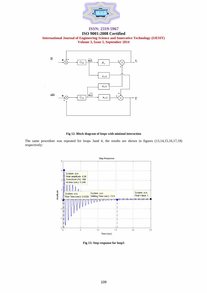
Fig 12: Block diagram of loops with minimal interaction

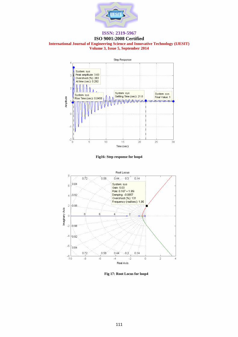
The same procedure was repeated for loops 3and 4, the results are shown in figures (13,14,15,16,17,18)

respectively:

Fig 13: Step response for loop3

ISSN: 2319-5967



110

Fig 14: Root Locus for loop3

Fig 15: Bode Plot for loop3

ISSN: 2319-5967



111

Fig16: Step response for loop4

Fig 17: Root Locus for loop4

ISSN: 2319-5967



112

Fig 18: Bode plot for loop 4

Table (7): comparison between the characteristic interacting loops (1, 2, 3, 4) using different techniques:

Method Routh Root Locus BodePlot

Loop1 Type of

controller

P PI PID P PI PID P PI PID

Kc 0.91 0.82 1.086 3.38 3.45 4.596 24.6 22.2 29.6

τi,sec - 5.02 3.01 - 1.88 1.125 - 1.8 1.08

τD,sec - - 0.753 - - 0.283 - - 0.27

Offset -0.136 - - -0.035 - - -0.01 - -

Loop2 Kc 1.66 1.494 21.9 12.85 11.565 15.42 16.93 15.24 20.32

τi,sec - 2.78 1.67 - 1.80 1.089 - 2.52 1.52

τD,sec - - 0.42 - - 0.27 - - 11.15

Offset -0.13 - - -0.007 - - -0.006 - -

Method Routh Root Locus BodePlot

Loop3 Type of

controller

P PI PID P PI PID P PI PID

Kc 1.52 1.368 1.824 1.865 1.679 2.238 0.988 0.889 1.186

τi,sec - 9.417 5.65 - 2.575 1.545 - 5.23 3.14

τD,sec - - 1.41 - - 0.385 - - 0.785

Offset -0.022 - - -0.017 - - -0.032 - -

Loop4 Kc 1.54 1.386 1.848 2.515 2.264 3.018 4.369 3.932 5.243

τi,sec - 3.232 1.939 - 2.683 1.61 - 2.727 1.636

τD,sec - - 0.485 - - 0.403 - - 0.409

Offset -0.021 - - -0.013 - - -0.007 - -

ISSN: 2319-5967



113

Table (8): Comparison between characteristic of the impulse responses

IV. DISCUSSION OF THE RESULTS

Interacting loops in the sour water stripper were identified, and their transfer functions were cited from the

literature. It was found that the feed rate affects the composition and temperature at the top of the column and

that the reflux ratio also affects the composition and temperature at the top of the column ,therefore the two

loops are interacting .It was also found that the flow rate of the residue affects the level at the base and the

temperature at the bottom of the column .It was observed that the steam rate affects the level and temperature at

the bottom of the column ,thus the two loops are interacting .The interaction of the interacting loops were made

to a minimum level using Relative Gain Array (RGA).The loops were coupled and it was seen that the

composition of the top of the column had to be coupled with feed rate and that the temperature had to be

coupled with the reflux ratio .It was decided that the level at the base of the column should be coupled with the

steam rate. Once the loops were coupled, stability and tuning analysis were carried out and the adjustable

parameter were obtained .These parameters were introduced in the overall transfer functions and the responses

were simulated for each loop and found to be stable with reasonable settling time and over shoot .The offsets

were investigated and compared against each in all loops and found to be within reasonable limits.

ACKNOWLEDGMENT

The authors wish to thank the college of Graduate Studies and Scientific Research, University of Science and

Technology for their help and support .This paper is generated from a Ph.D. thesis in Chemical engineering.

REFERENCES [1] Jin Shang jun., “Sour Water stripping unit operation procedure”, KRCmanual, 2010.

[2] Katsuhiko O., “Modern Control Engineering”, Prentice Hall. Fifth edition, 2010, New Gersy.

[3] Stephanopoulos, G., “Chemical process control, an introduction to theory and practice”, Prentice Hall of India Private

limited, New Delhi, 2005.

[4] Carlos A., “Principles and practice of Automatic Process Control”, John Wiley and sons Inc, Asia edition, 2006.

[5] Roland S., “Advanced control engineering”, Butterwoth-Heinemann, Oxford, 2001.

[6] Gasmelseed, G.A. “Advanced control for graduate students”, G-town, Khartoum, 2012.

Character Loop1 Loop2 Loop3 Loop 4

Amplitude 1.42 2.42 4.06 3.63

Overshoot 64.5 166 306 263

Settling time 12.5 22.5 15.5 21.8

Rise time 0.699 0.304 0.0326 0.458

Documents

ISSN: 2319-5967 ISO 9001:2008 Certified International ... 3/Issue 5/IJESIT201405_10.pdf · tedious .In the sour water stripping column in ... of the loops and then design ... as condensates