Embed Size (px)
Citation preview
DESIGN AND CONSTRUCTION OF A PULSE FORMING
NETWORK, PULSE TRANSFORMER POWER SUPPLY
FOR THE TEXAS TECH RAILGUN
by
MICHELE WOFFORD, B.S.
A THESIS
IN
ELECTRICAL ENGINEERING
Submitted to the Graduate Faculty of Texas Tech University in
Partial Fulfillment of the Requirements for
the Degree of
~~STER OF SCIENCE
IN
ELECTRICAL ENGINEERING
Approved
Accepted
August, 1991

ACKNOWLEDGMENTS
I would like to thank the pulsed power staff and
students, who helped me run this project as smoothly as
possible. Danny and Dino, your hard work and effort made
this project possible, and I could not have asked for better
help. Michael, it has been fun working with you, good luck
with your future endeavors. Dr. Giesselmann deserves credit
for his advice and information about the pulse transformer.
Dr. Baker, thank you for being such a patient and
encouraging advisor.
I want to thank Dr. Glen McDuff and Dr. Tom Burkes,
whose faith and guidance inspired me to go to graduate
school. Last, but most certainly not least, I cannot
overemphasize the interest and support of my family
throughout my education, I love you.
ii

TABLE OF CONTENTS
ACKNOWLEDGMENTS • . . • • • • . . . • • • . . • • • ii
ABSTRACT . . . . . . . . . . . . . . . . . . . . . . . . v
LIST OF TABLES . . . . . . . . . . . . . . . . . . . • • vi
LIST OF FIGURES • . . . . . . . . • • • • • • • • . . . vii
CHAPTER I INTRODUCTION ••••••••••••••••• 1 The Direction of Railgun Research ••••••• 2 Railgun Operating Theory ••••••••••. 4
Electromagnetic Theory. • • • • • • • .5 Plasma Armatures • • • • • • • • • • • • 7
CHAPTER II POWER SUPPLY AND DIAGNOSTIC THEORY • • • • • 10 Railgun Equivalent Circuit • • • • • . • 11 Power supply Design Background • . • • • • • 13
Monocyclic Power Supply Background • 14 Pulse Forming Network Background •••• 17 Pulse Transformer Background • • • • • • 20 Ignitron Background • • • • • . • • • • • 23
Diagnostics. • • • • • • • • . • • . . • . • 24
CHAPTER III DESIGN AND CONSTRUCTION OF THE HERA POWER SUPPLY AND DIAGNOSTICS • • • • • • • • • • • 27 Monocyclic Power supply Design • • • . • • • 27 PFN Design • • • • • . • • • • • . • . • • • 29 Transformer and Switching Circuitry ••••• 30 Mechanical Design. • • . . • • • • • . • • • 33
High-current Buswork. • • • • • • • • • • 33 Pre-Injector Gas Gun. • • . • • • • • . • 36 Railgun • • • • • • • • • • • • • • • • • 37
controls and Diagnostics • • • • • • • . 39 LeCroy Data Acquisition System. • • • • • 40 Optical Trigger for Iqnitron. • • • • 40
CHAPTER IV EXPERIMENTAL RESULTS • • • • • • • • • • • • 43
CHAPTER V
PFN Testing • • • • • • • • • • • • • • • • 43 PFN Into an Iqnitron Load • • • • • • • • 43 PFN Into Railgun Load • • • • • • • • • • 53
Pulse Transformer Testing •••••••••• 55 Pulse Transformer Model • • • • • • • • . 55 Pulse Transformer Tests • • • • • • • • • 56
High current Testing Into the Railgun. . • • 60 Velocity Measurements • • • • • • • • • • 69
CONCLUSIONS. • • • • • • . . . . . . . . • • 72
iii

REFERENCES
APPENDIX. •
• •
• •
• • • • • • • •
• •
iv
•
•
• 75
77

ABSTRACT
A pulse forming network (PFN), pulse transformer power
supply has been designed, constructed, and tested to supply
high current for the Texas Tech railgun. The power supply
can deliver 500 kA to 1 MA for almost 1 ms to the railgun
load. The current level is dependent upon the charge
voltage of the PFN and the turns ratio of the transformer.
The PFN is a Type E and has five stages. Comprised of
11 kV, 50 kJ Maxwell capacitors, the capacitor bank can
supply a total of 500 kJ at 10 kV. The PFN is designed to
deliver 100 kA at half voltage, or 200 kA for the full 10
kV. The total current delivered to the railgun depends on
the transformer ratio, which can be altered from 5:1 to
10:1.
This type of power supply is unique for railgun loads.
Generally, homopolar generators or distributed capacitor
banks have been used. PFNs have been used to drive
railguns, but without the pulse transformer. The addition
of the transformer increases the power transfer efficiency,
and boosts the current without affecting the pulse length.
The advantages of this system are as follows: it provides
high constant current without complex controls, the output
current can be increased without changing the system, and
the PFN waveform is tunable.
v

4.1.
4.2.
LIST OF TABLES
PFN Peak currents for Ignitron Load Tests
Pulse Transformer Values • • • . . . . . .
vi
• • • • 53
. . . • 55
1.1.
1.2.
2.1.
2.2.
2.3.
2.4.
2.5.
2.6.
2.7.
2.8.
3.1.
3.2.
3.3.
3.4.
LIST OF FIGURES
Propulsion Mechanism in Railguns . . . . . . . . 6
Four-Stage Plasma Armature Model
Railgun Equivalent Circuit. • • • •
Power Supply and Load Waveforms . . R-C Charging Network . . . . . . .
. . . . . . 8
. . . . • • • 12
• • . . . . • 13
. . . . . . • 15
Monocyclic Power supply • . . . . . . . . . . • • 16
Type E Pulse Forming Network . . . . . . . . • • 19
Ideal Transformer Model • • • . . . . . . . . . • 21
Non-Ideal Transformer Model . • • 22
Placement of B-Oot Probes • • . . . . . . . • • • 25
Block Diagram of Power Supply • . . . . . . • 28
Texas Tech Railgun PFN . . . . . . . . . . • 30
Transformer Turns Ratios . . . . . . . . . . . • 31
Pre-Injector Gas Gun . . . . . . . • 37
3.5. Pre-Injector Gun Poppet Valve Operation .•••• 38
3.6. Railgun Bore Cross Section. . . . . . . . . . 39
3.7. optical Trigger Setup • . • . . . . . • . 41
3.8. Timing Diagram of Triggering Scheme . . . . . 42
4.1. Total PFN current for a 5 kV Charging Voltage into an Ignitron Load. • • • • • • • • • • • • • • 45
4.2. Capacitor current for Each Stage for a 5 kV Charging Voltage into an Ignitron Load. • • • • . 46
4.3. Inductor current for Each Stage for a 5 kV Charging Voltage into an Ignitron Load . • • 47
4.4. Diode current for Each stage for a 5 kV Charging Voltage into an Ignitron Load • • • • . . • • • 48
vii
4.5. stage 1: Capacitor current . . • . • . . . • • . 49
4.6. Stage 2: Capacitor current . . . . . . . . . • . 49
4.7. stage 3: Capacitor current . • . . . . . . • . . 50
4.8. Stage 4: Capacitor current . . . . . . . . . . . 50
4.9. Stage 1: Diode current . . . • • • • • . • • • . 51
4.10. Stage 2: Diode current . . • • • • • • . . . 51
4.11. Stage 3: Diode current . . . • • . • • . 52
4.12. Stage 4: Diode current • . • . • . • . . • . . • 52
4.13. Railgun Current for a 2 kV Charging Voltage . . . 54
4.14. Transformer Performance for 5:1 Turns Ratio into a Matched Load • • • • • • • • • • • • • • • • . 57
4.15. Transformer Performance for 10:1 TUrns Ratio into a Matched Load . • • • • • • . . . • • • • • • • 58
4.16. Transformer Test into a Short Circuit Load .•. 59
4.17. PFN and Railgun currents for a Matched Resistive Load . . • . . . . . . . . . . . . . . . . . . . 61
4.18. PFN and Railgun currents for Ideal Buswork Resistance and Inductance, Breech Voltage Load • 62
4.19. Buswork Contact Resistance Effect on PFN and Railgun Currents • • • . • • • • • • • • • • • . 63
4.20. Railgun Inductance Effect on PFN and Railgun Currents . . . . . . . . . . . . . . . . . . . . 6 4
4.21. Buswork Contact Resistance and Railgun Inductance. Effects on PFN and Railgun currents • • • • • • • 65
4.22. Fuse Shot: PFN current for 2 kV Charging Voltage 67
4.23. Fuse Shot: PFN current for 5 kV Charging Voltage 67
4.24. Fuse Shot: Breech Voltage for 5 kV Charging Voltage •• . . . . . . . . . . . . . . . . . • • 68
4.25. Projectile Shot: PFN current and Breech Voltage for 5 kV Charging Voltage • • • • • • • • • • • . 68
4.26. Fuse Shot: B-dot Waveforms for Probes 1 and 2 •• 70
viii

4.27. Fuse Shot: B-dot waveforms for Probes 2 and 3 •• 70
ix

CHAPTER I
INTRODUCTION
This thesis describes the design, construction, and
testing results of a high-current power supply for the Texas
Tech High Energy Railgun Accelerator (HERA) railgun. The
power supply can deliver a single-shot, constant-current
pulse to the railgun in the range of 500 kA to 1 MA for a
time period of about 1 ms. The power supply consists of a
monocyclic charging power supply, a Type E pulse forming
network (PFN), an ignitron switch, and a pulse transformer.
Chapter II discusses the theory and design considerations of
each part of the power supply and the appropriate
diagnostics. Chapter III describes the design and
construction of the power supply, including the high-current
buswork from the transformer to the railgun. The testing
results and conclusions are presented in the last two
chapters.
several different sources, discussed in Chapter II, are
used to drive the low-impedance railgun load. PFNs have
been used sparingly for this application because the PFN
impedance is generally mismatched to the load. The
subsequent oscillations are detrimental to the energy
storage capacitors used in the PFN. Also, the design of the
characteristic impedance of the PFN is dependent on the
pulse length. Lowering the impedance will generally lower
1
the pulse length, and railgun loads require high currents
for a relatively long period of time. The dependence of the
impedance and pulse length are apparent from the design
equations in the PFN background section of Chapter II.
However, PFNs have the following advantages: the pulse
shape can be designed for linear or nonlinear loads, the
pulse shape can be tuned over a limited range, and the pulse
width can be tailored to the specific needs of the load.
This particular power supply is unique because it utilizes
the advantages of the PFN and overcomes the disadvantage of
the impedance mismatch by using a pulse transformer. The
transformer serves a dual purpose; it boosts the PFN current
without compromising the pulse length, and provides a better
impedance match to the railgun load.
The Direction of Railgun Research
The velocity of a conventional gun is limited by the
thermodynamics of the expanding gas within the bore.
Electromagnetic launchers, or railguns, discussed in detail
in the following section, do not have this limitation and,
theoretically, much higher velocities can be obtained.
Consequently, the kinetic energy of the projectile is
increased as a result of higher velocity.
Experiments have shown that the basic theory of
railguns is correct. However, experiments have also shown
an anomaly called velocity saturation, where increasing the
2

input energy does not increase the velocity. In early
experiments that used solid conducting armatures, the
velocity was limited to less than 2 kmjs. Apparently, as
the solid armature moved down the bore, the electrical
contact between the armature and rails decreased, thereby
limiting the energy transferred to the projectile.
Research then focused on plasma armatures, which have
the advantage of smaller mass, better electrical contact,
and less rail erosion than solid armatures [1]. Research
has concentrated mainly on plasma armatures after the
successful experiment at the Australian National University
in 1977. From this experiment, s.c. Rashleigh and R.A.
Marshall concluded that larger railgun systems should
produce higher velocities [2]. However, few experiments
have exceeded the 5.9 km/s obtained in Australia.
Most researchers agree that a secondary arc behind the
armature causes the velocity saturation. Instead of all the
energy being directed at the projectile, some is wasted in a
parasitic arc that forms well behind the armature. The
formation of the secondary arc is not completely understood,
mainly because a complete model of the plasma armature does
not exist. However, the restrike is believed to happen in a
sequence of events, which will be explained in detail later
in this chapter.
Research at Texas Tech University will focus on the
development of hybrid armatures, plasma armatures that are
3

continually "seeded" with conductive material [3]. The
hybrid armature will serve a dual purpose. First, the
plasma will not have to strip the rails for conducting
material to maintain high conductivity. Secondly,
experiments have shown that the plasma lengths tend to be
more localized if the plasma is seeded.
The armature of the Tech railgun will be seeded by a
thick fuse at the back of the projectile, rather than
injecting the material into the bore during a shot. With
this approach, the added material is in the appropriate
frame of reference and velocity. Also, the amount and type
of material may be more carefully controlled. Ongoing
research will be performed to determine plasma properties
and the effect of the hybrid armature. This thesis will
focus on the operating system that will enable this research
to begin.
Railgun Operating Theory
Railgun structures are relatively simple~ they consist
of conducting rails, an armature (which is generally part of
the projectile), and a support structure. A large support
structure is required because the forces generated in the
gun tend to blow the rails apart.
4
Electromagnetic Theory
Railguns operate on the theory of the Lorentz force in
Equation 1.1
F = q(E + v X B) N (1.1)
where q = electric charge, E = electric field, v = particle
velocity, and B = magnetic field. since the primary driving
force is a powerful magnetic field, the effects of the
electric field are neglected, and the governing equation,
derived from Equation 1.1, is
dF = dl (I X B) N m
(1.2)
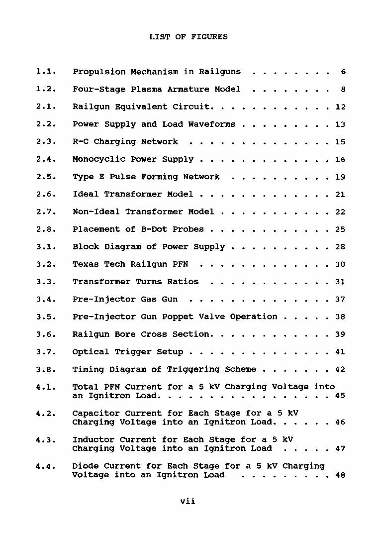
where dl = elemental length. As pictured in Figure 1.1, the
rail current interacts with the armature magnetic field to
generate the force. Not only does the armature provide a
current path between the rails, but it supplies a medium to
transfer the magnetic energy into kinetic energy. The
magnetic field between the rails, determined by Ampere's
law, is
- I I B = J.Lo ( d) W+
T (1.3)
where w = width and d = height of each rail. Integrating
Equation 1.2 with the magnetic field in Equation 1.3 results
in
5

where L' equals
L' s = ~0 w + d H m
(1.4)
(1.5)
where s = separation between rails. For this railgun, L' =
.592 uHjm.
..Jarc ..Jarc x Bra i Is
Ira i I
Figure 1.1 Propulsion Mechanism in Railguns
After calculating the force due to the magnetic field,
the acceleration, velocity, and position of the projectile
can be predicted. These terms are calculated respectively
in Equations 1.6 through 1.8.
a =
6
m g2
(1.6)
If the mass of the projectile, m, and system current is
known, the acceleration may be determined. If the current
delivered to the railgun is constant, which it is in this
case, the acceleration is constant: therefore, the velocity
is linear.
v(t) = (tia L' dt + v(O) Jo 2m
m s
(1.7)
The position of the projectile in the bore is determined
simply be integrating the velocity with respect to time.
x( t) = x(O) + v(O) t + ( t I2
L' t dt m . Jo 2m
(1.8)
Plasma Armature
The losses associated with the transfer of energy from
the armature to the projectile are the main limitations of
railguns. Once the loss mechanisms are well understood,
steps can be taken to increase the efficiency of the system.
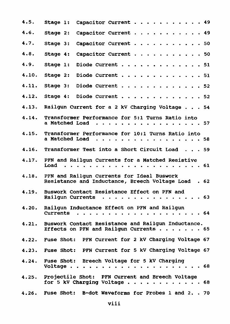
J.V. Parker presents a thorough, .up-to-date examinations of
plasma armature behavior in Reference [4]. Assuming the
plasma has moved far enough for restrike conditions to
occur, Parker divides the armature into four regions as can
be seen in Figure 1.2.
The main, or primary, plasma is extremely hot and
highly ionized. The plasma ablates material from the bore
rails and insulators, and this material starts to lag behind
7
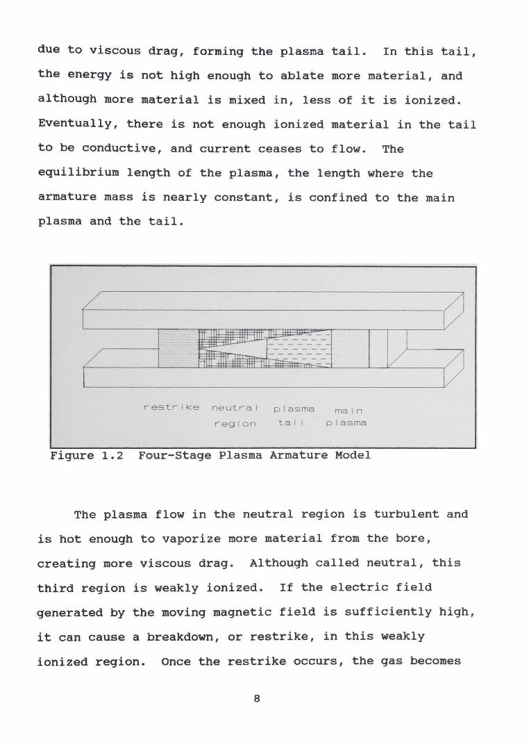
due to viscous drag, forming the plasma tail. In this tail,
the energy is not high enough to ablate more material, and
although more material is mixed in, less of it is ionized.
Eventually, there is not enough ionized material in the tail
to be conductive, and current ceases to flow. The
equilibrium length of the plasma, the length where the
armature mass is nearly constant, is confined to the main
plasma and the tail.
restrike neutral plasma main
region tai I plasma
Figure 1.2 Four-Stage Plasma Armature Model
The plasma flow in the neutral region is turbulent and
is hot enough to vaporize more material from the bore,
creating more viscous drag. Although called neutral, this
third region is weakly ionized. If the electric field
generated by the moving magnetic field is sufficiently high,
it can cause a breakdown, or restrike, in this weakly
ionized region. Once the restrike occurs, the gas becomes
8

highly ionized and conditions are favorable to sustain the
parasitic arc. As more current is shunted into the
secondary arc, less energy is available to propel the
projectile. The tail and neutral regions of the armature
are not as well understood as the main plasma. Research on
the HERA railgun will be centered around determining the
characteristics of these regions and overcoming the
difficulties they produce.
9

CHAPTER II
POWER SUPPLY AND DIAGNOSTIC THEORY
Several factors are important for a railgun power
source. The source should provide a high constant current
to generate the large forces in the gun and maintain the
acceleration. Also, the source should be designed such that
a minimum amount of energy is wasted in a muzzle flash when
current attempts to flow into the gun after the projectile
has exited. Therefore, the amplitude and shape of the
current pulse are important considerations.
Power sources that can generate the high currents
necessary for railgun operation are the homopolar generator,
inductive energy storage, capacitor banks, distributed
energy systems, batteries, and pulse forming networks [5].
Homopolar generators can store a large amount of energy and
produce very high currents. However, the output voltage is
generally low, and it is difficult to stop the current flow
once the projectile exits the railgun. High losses and
technical complications associated with opening switches
make inductive energy storage an unattractive alternative.
Large capacitor banks can store quite a bit of energy but
have no means of pulse shaping. Distributed capacitor banks
are placed along the length of the gun instead of being
placed only at the breech of the gun. The distributed bank
has the advantage of reduced I 2R losses and more control of
10
the pulse shape, but it requires precise timing of multiple
switches. Batteries are an inexpensive way to store energy,
but they cannot provide pulse shaping. The pulse forming
network, or PFN, can deliver a constant current for a
controlled length of time and does not require complex
controls. If the PFN impedance matches the load impedance,
all of the energy stored in the PFN can be delivered to the
load. If the pulse length coincides with the timing of the
projectile exiting the gun, and the circuit losses are low,
the efficiency can be very high.
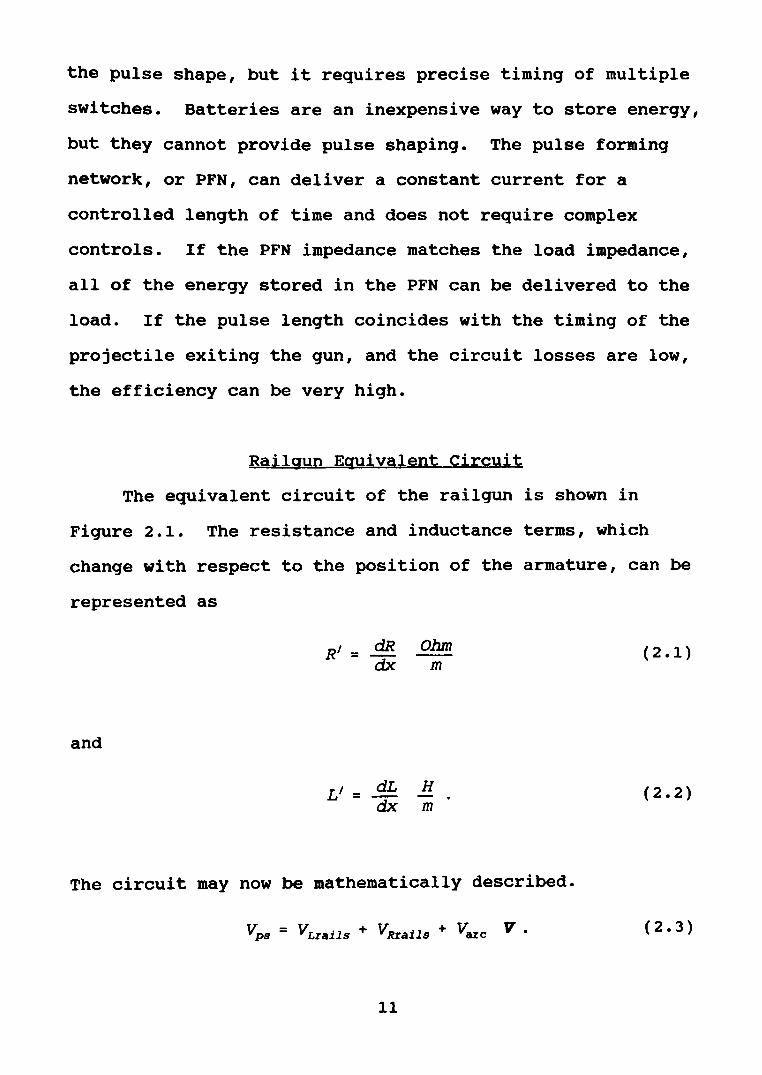
Railgun Equivalent Circuit
The equivalent circuit of the railgun is shown in
Figure 2.1. The resistance and inductance terms, which
change with respect to the position of the armature, can be
represented as
and
R' = dR Ohm dx m
L' = dL H dx m
The circuit may now be mathematically described.
vps = VLrails + v Rrails + varc v .
11
(2.1)
(2.2)
(2.3)
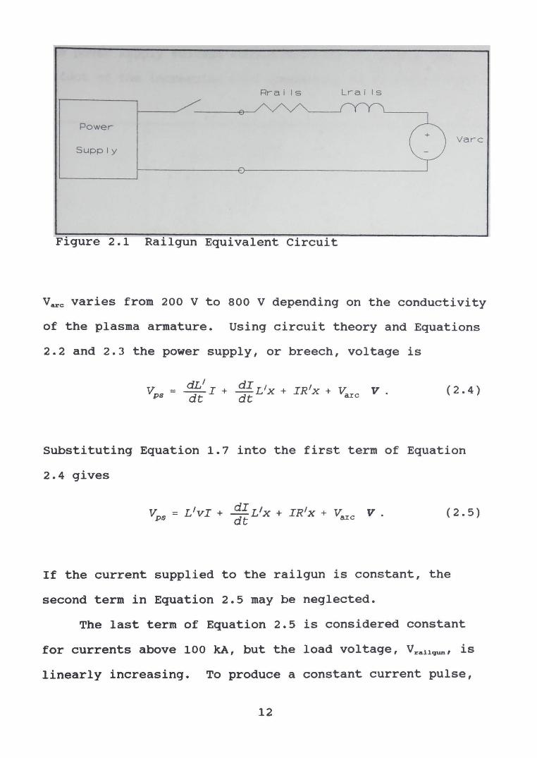
- -Rra i Is Lra i Is
0 A
Power
0 Varc Supply
,...... '-'
. . . F1gure 2.1 Ra1lgun Equ1valent Circuit
V~e varies from 200 V to 800 V depending on the conductivity
of the plasma armature. Using circuit theory and Equations
2.2 and 2.3 the power supply, or breech, voltage is
V dL' I + di L 1x + IR1x + V V ps = dt dt arc '
(2.4)
Substituting Equation 1.7 into the first term of Equation
2.4 gives
V = L 1vi + di L 1x + IR1x + V V ps dt arc •
(2.5)
If the current supplied to the railgun is constant, the
second term in Equation 2.5 may be neglected.
The last term of Equation 2.5 is considered constant
for currents above 100 kA, but the load voltage, Vrau.qunt is
linearly increasing. To produce a constant current pulse,
12
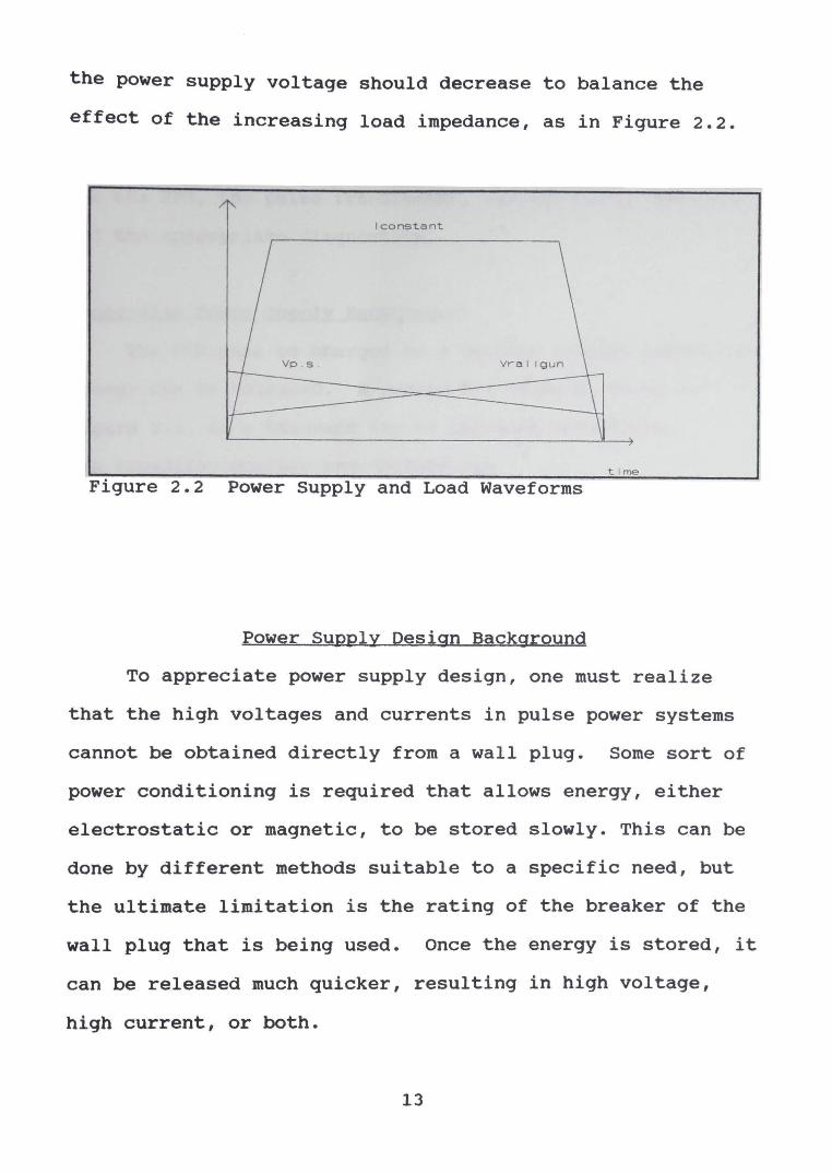
the power supply voltage should decrease to balance the
effect of the increasing load impedance, as in Figure 2.2.
I constant
Vra 1 I gun
time
Figure 2.2 Power Supply and Load Waveforms
Power Supply Design Background
To appreciate power supply design, one must realize
that the high voltages and currents in pulse power systems
cannot be obtained directly from a wall plug. Some sort of
power conditioning is required that allows energy, either
electrostatic or magnetic, to be stored slowly. This can be
done by different methods suitable to a specific need, but
the ultimate limitation is the rating of the breaker of the
wall plug that is being used. Once the energy is stored, it
can be released much quicker, resulting in high voltage,
high current, or both.
13
In this case, a system is designed for high-current,
single-shot operation. The remainder of this chapter will
discuss the theory and design of the driving power supply
for the PFN, the pulse transformer, the switching circuitry,
and the appropriate diagnostics.
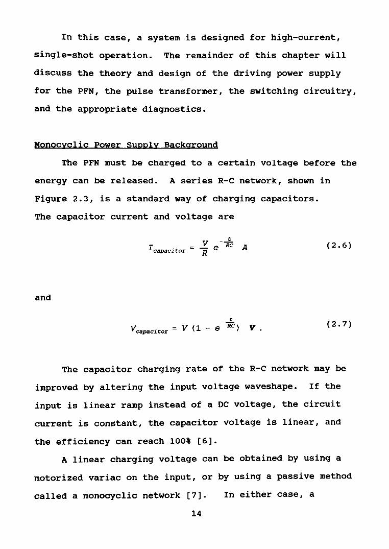
Monocyclic Power Supply Background
The PFN must be charged to a certain voltage before the
energy can be released. A series R-C network, shown in
Figure 2.3, is a standard way of charging capacitors.
The capacitor current and voltage are
I capacitor =
and
t
V V (1 e -Re) capaci t:or = - v.
(2.6)
(2.7)
The capacitor charging rate of the R-C network may be
improved by altering the input voltage waveshape. If the
input is linear ramp instead of a DC voltage, the circuit
current is constant, the capacitor voltage is linear, and
the efficiency can reach 100% [6].
A linear charging voltage can be obtained by using a
motorized variac on the input, or by using a passive method
called a monocyclic network [7]. In either case, a
14
constant current is supplied. This thesis will focus on the
monocyclic method.
Rcharge
~ ~ D C . l Ccharge
Power Supply T
Figure 2.3 R-C Charging Network
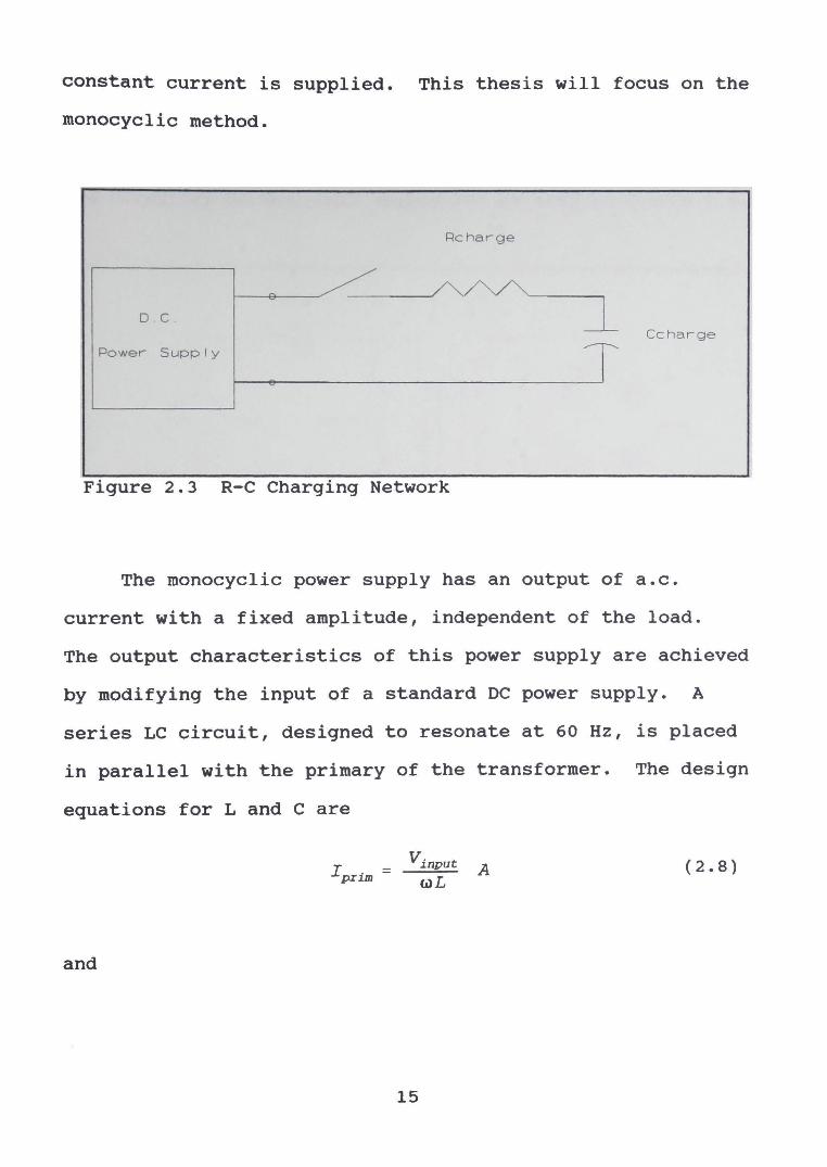
The monocyclic power supply has an output of a.c.
current with a fixed amplitude, independent of the load.
The output characteristics of this power supply are achieved
by modifying the input of a standard DC power supply. A
series LC circuit, designed to resonate at 60 Hz, is placed
in parallel with the primary of the transformer. The design
equations for L and c are
and
I . = prl.lll (2.8)
15
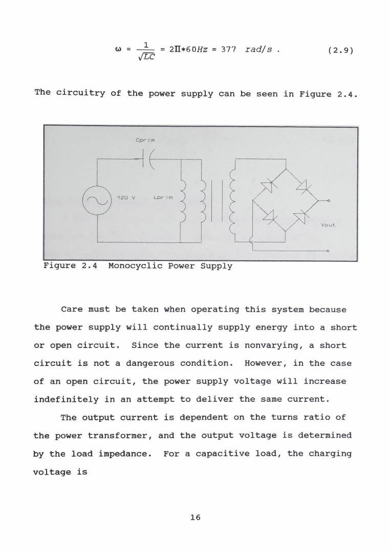
(a) = 1
v'LC (2.9) = 2IT•60Hz = 377 rad/ s .
The circuitry of the power supply can be seen in Figure 2.4.
Cprrm
Figure 2.4 Monocyclic Power Supply
Care must be taken when operating this system because
the power supply will continually supply energy into a short
or open circuit. Since the current is nonvarying, a short
circuit is not a dangerous condition. However, in the case
of an open circuit, the power supply voltage will increase
indefinitely in an attempt to deliver the same current.
The output current is dependent on the turns ratio of
the power transformer, and the output voltage is determined
by the load impedance. For a capacitive load, the charging
voltage is
16

1 L t 'd vc = - ~ t v. c 0 (2.10)
For a constant current, the charging time for a specific
voltage is
cv I
Pulse Forming Network Background
s. (2.11)
A PFN will supply the high current and pulse shaping
necessary for this project. PFNs can be designed for
complex loads; however, the scope of this project is limited
to the design of a PFN for a resistive load. The PFN can be
tuned to fit the more specific needs of this project. This
can be a separate project, and a good reference is [8].
Pulse forming networks are lumped parameter
approximation of a transmission line. A lossless
transmission line can deliver a square pulse to a matched
load. The length, geometry, and material of the line
determine the propagation time,
(2.12)
where er = relative permitivitty and c = speed of light.
The characteristic impedance of a pulse forming line is
17
(2.13)
The pulse length is twice the one way transit time, T1 wav•
Cable transmission lines make simple pulsers but have
several disadvantages. For pulses longer than several
nanoseconds, the cable length becomes too long to be
practical. Also, there are limited impedances available and
the cable stores a limited amount of energy.
Whereas a transmission line is modelled as a
distributed network of inductors and capacitors, a PFN is a
lumped parameter network with a finite number of elements
that approximates transmission line behavior. The advantage
of a PFN is that the characteristic impedance and pulse
length are dependent on component values and are flexible.
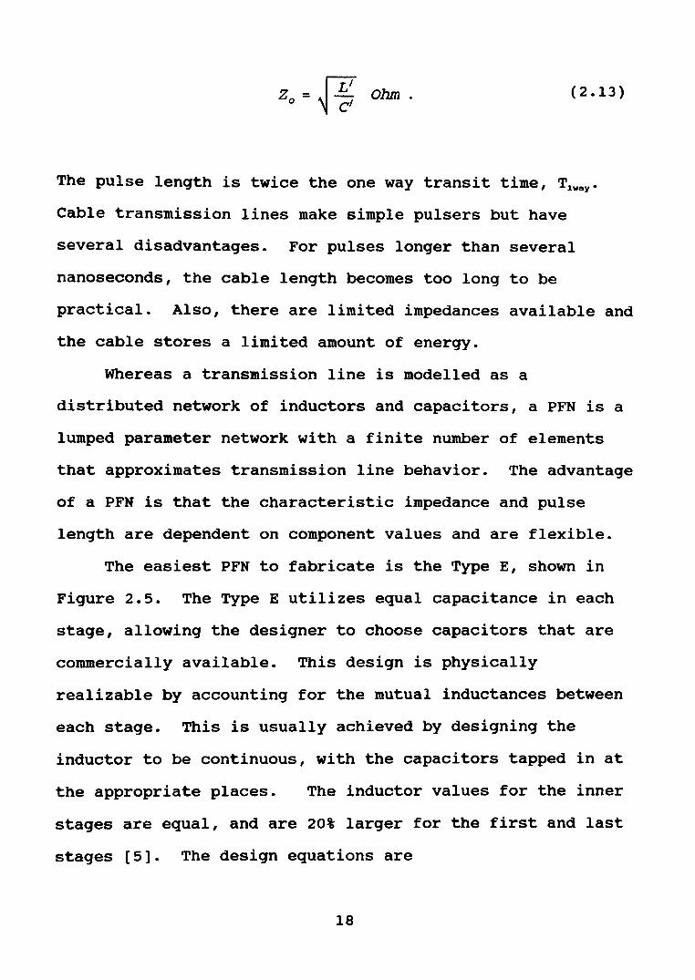
The easiest PFN to fabricate is the Type E, shown in
Figure 2.5. The Type E utilizes equal capacitance in each
stage, allowing the designer to choose capacitors that are
commercially available. This design is physically
realizable by accounting for the mutual inductances between
each stage. This is usually achieved by designing the
inductor to be continuous, with the capacitors tapped in at
the appropriate places. The inductor values for the inner
stages are equal, and are 20% larger for the first and last
stages [5]. The design equations are
18
and
z = 0 v
2I = Ltotal
ctotal Ohm (2.14)
(2.15)
·---
_Crvv\_Crvv\_Crvv\(\~
L C1 T C2 T C3 T C4 J cs
C1 = C2 = C3 = C4 = CS
Figure 2.5 Type E Pulse Forming Network
If the inductor is a solenoid and the turns are equally
spaced, the design equation is
Lsolenoid = (2.16)
where N =number of turns, U0 = permeability of free space,
A = cross sectional area, and 1 = length of solenoid. This
is a rough approximation, excluding the effects of mutual
inductance. The buswork and railgun have significant
19

inductance, so an approximation of the PFN inductor value is
sufficient.
Pulse Transformer Background
Transformers are used to step up voltage or current, to
match impedances, to invert signals, or to isolate the load
from the source. Pulse transformers are a class of
transformers that are designed for pulse applications. This
has a definite impact on the design and layout of the
transformer.
First, a few properties will be defined to further the
discussion. In a pulse transformer, the primary and
secondary inductances are wound close together, so the
geometry of each is approximately the same. Therefore, the
value of the primary and secondary are related through the
turns ratio, N by
(2.17)
Mutual inductance, M, is a measure of the flux linkage of
the two inductors. It is related to the coupling
coefficient, k, by
(2.18)
coupling coefficient, which ranges from O<k<1, is a measure
of the percentage of flux linkage from the primary to the
20
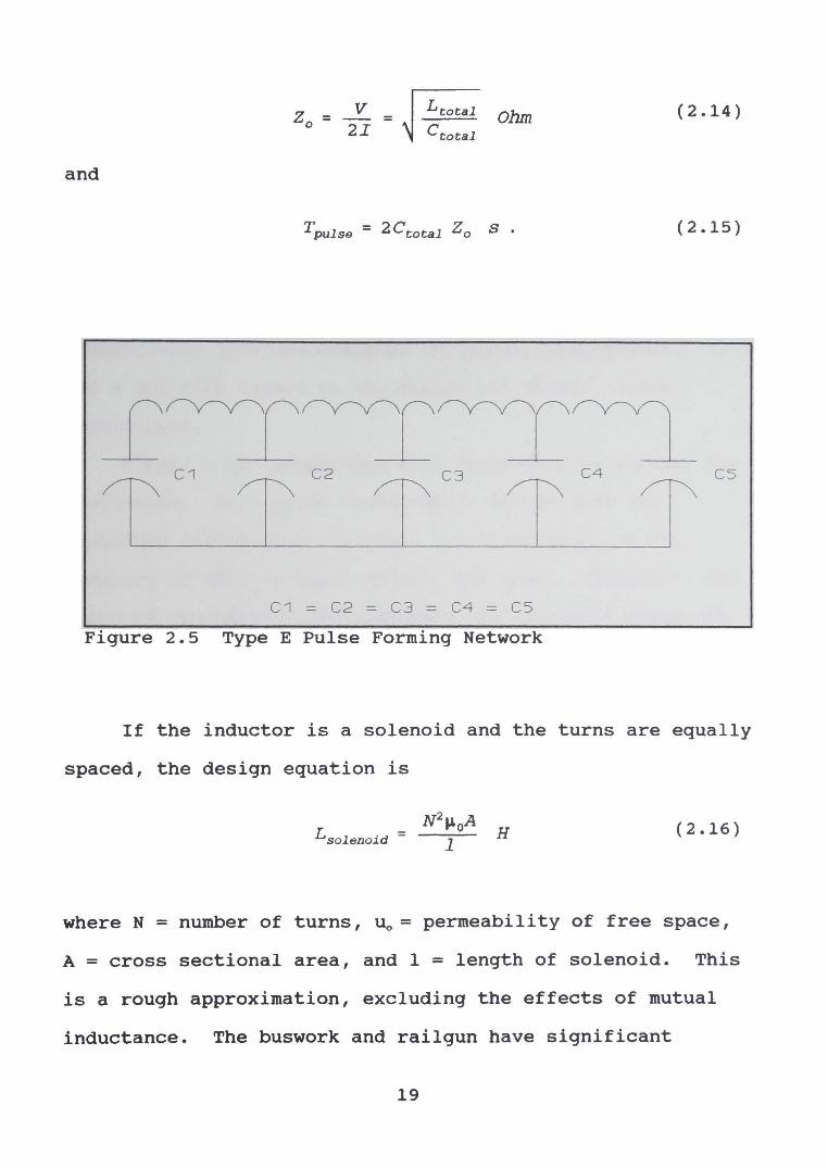
secondary of a transformer. The perfect transformer would
have k=l, which means all of the flux from the primary is
linked to the secondary. In an ideal transformer, no energy
resides in the core of the transformer, which is assumed to
have infinite permeability. The model of the ideal
transformer can be seen in Figure 2.6.
V1 N1 N2 V2 N2/N1 ~ V1
Figure 2.6 Ideal Transformer Model
Transformers differ from the perfect model due to
losses associated with an iron core and with the windings.
Core losses are the result of energy lost in the hysteresis
process and eddy currents. Also, a small amount of current
is needed to overcome the reluctance of the core. These
losses are represented as the excitation current, which is a
sum of the core-loss and magnetizing currents. The finite
resistance of the windings and the loss of flux linkage from
the primary to secondary create the leakage losses. When
21
maximum coupling is desired, k approaches 1, and the losses
are kept to a minimum.
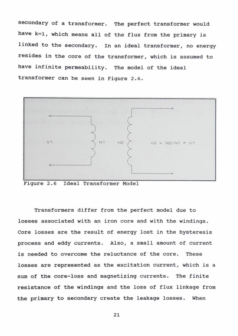
The losses due to the iron core and windings can be
represented as circuit values in the transformer model.
Core losses are represented as R~r• and L_9 , which are in
parallel to the primary. Winding losses, in series with the
model, are represented as R.,1n., and L1.ak. There is also a
distributed capacitance which results from the separation of
the high voltage windings from ground. Figure 2.7 fully
represents the transformer model.
Lleak Rwlnd
Lleak Rwlnd
V'1 V2
Figure 2.7 Non-Ideal Transformer Model
A correctly designed pulse transformer will retain the
pulse shape of the primary signal. To retain pulse shape,
the rise and fall time of the pulse should not be degraded,
there should be minimal overshoot and droop, and the core
22
should not saturate. Designing a transformer to handle high
power, pulse conditions is not an elementary problem. A
more detailed description is given in Reference [9].
Ignitron Background
Ignitrons are mercury vapor vacuum switches that are
designed to handle high currents. To turn the ignitron on,
a fast, high voltage pulse is applied to the ignitor pin,
which vaporizes a small portion of the cathode mercury pool.
The vapor creates a conducting path, that the energy
released into the switch sustains. once the current flowing
through the ignitron becomes negligible, the mercury vapor
recombines and condenses, and the switch turns off.
Although an ignitron is a relatively easy switch to
operate and maintain, several steps must be taken to use the
switch properly. The voltage pulse applied to the ignitor
pin should be a minimum of about 1 kV, and the polarity
should be positive with respect to the cathode. A negative
voltage can short out the ignitor. Also, even if the
ignitor is pulsed, the switch will not fire unless there is
a potential difference of around 1 kV across the anode and
cathode. Also, current reversal should be kept to a minimum
to maximize the lifetime of the tube. The switch must be
mounted vertically, otherwise the cathode mercury pool will
short to the anode. In addition, the temperature of the
sidewalls and the anode should be kept above the temperature
23

of the mercury pool to prevent prefire. All of this
information should be taken into consideration when
electrically and mechanically designing an ignitron into a
circuit.
Diagnostics
The main data to be taken for this project is the
current amplitude and waveshape delivered to the railgun,
the muzzle voltage, and the velocity of the projectile as it
travels and exits the bore. The first two will help
characterize the power supply and the railgun. This
information will be compared to predicted responses on
PSPICE, a circuit simulation program. The velocity
measurements will help determine if and where velocity
saturation is taking place. In the future, the tail of the
plasma armature will be characterized by data gathered from
microwave interferometry. This information can be coupled
with velocity measurements to determine the causes of the
saturation effect.
B-dot probes placed along the outer bore of the gun
will be used to determine the velocity of the projectile as
it travels down the bore of the railgun. B-dot probes
generate a voltage proportional to the time derivative of a
magnetic field. The voltage induced is given by
24
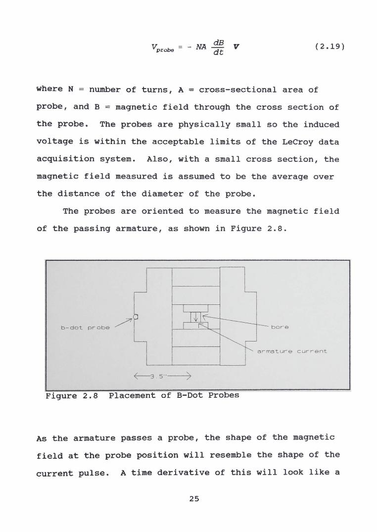
dB Vp.rabe = - NA dt V {2.19)
where N = number of turns, A = cross-sectional area of
probe, and B = magnetic field through the cross section of
the probe. The probes are physically small so the induced
voltage is within the acceptable limits of the LeCroy data
acquisition system. Also, with a small cross section, the
magnetic field measured is assumed to be the average over
the distance of the diameter of the probe.
The probes are oriented to measure the magnetic field
of the passing armature, as shown in Figure 2.8.
b-dot probe ~ bore
armature current
~3 . 5" )
Figure 2.8 Placement of B-Oot Probes
As the armature passes a probe, the shape of the magnetic
field at the probe position will resemble the shape of the
current pulse. A time derivative of this will look like a
25

negative spike representing the rising edge, a positive
spike representing the falling edge, and the zero-crossing
representing the maximum field. The maximum magnetic field
corresponds to the maximum current of the armature.
Coupling the knowledge of the zero-crossing times of each
probe with the known distance between each probe, velocity
measurements can be made for the length of the gun.
26

CHAPTER III
DESIGN AND CONSTRUCTION OF THE HERA
POWER SUPPLY AND DIAGNOSTICS
The design criteria for this project was to have a
power conditioning system to convert a.c. line voltage into
a pulsed power system that could deliver up to 500 kJ of
energy in a single pulse. The designed power supply
converts a single-phase, 220 V wall connection into a 500 us
single shot pulse. The system is flexible and can deliver
from 500 kA to 1 MA by increasing the charge voltage on the
capacitor bank of the PFN, or by altering the turns ratio of
the pulse transformer. The power supply consists of a
constant current power supply, a pulse forming network, an
ignitron switch, and a pulse transformer.
This chapter will discuss the electrical and mechanical
design of the power supply and the diagnostics system. A
block diagram of the power supply can be seen in Figure 3.1.
Monocyclic Power Supply Design
The primary circuit values are L=.06 H and C=120 uF,
and from Equation 2.8, the peak sinusoidal primary current
is 9.72 A. The transformer has a 1:45 ratio, and can handle
a maximum power of 37 kVA. Given the input circuit and a
220 v single-phase voltage, the peak secondary current is .2
A. The secondary of the transformer is connected to a full-
27
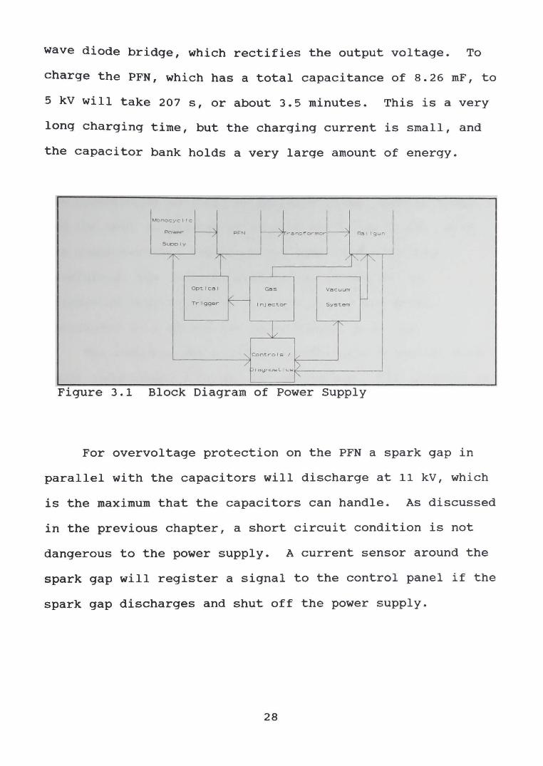
wave diode bridge, which rectifies the output voltage. To
charge the PFN, which has a total capacitance of 8.26 mF, to
5 kV will take 207 s, or about 3.5 minutes. This is a very
long charging time, but the charging current is small, and
the capacitor bank holds a very large amount of energy.
Mc-nccyc 1 T c
!=In WAr -7 PFN 7 renc1'ormcr ~ Ral lgun /
Suoolv
/f". T 1"7 ", I
Op1:1Cal Gas Vacuum
Tr-Igger ~ Injector System
,1 /f'
' Controls I /
/ Dl d.'JIIO!=o L I Lb l>
I'
F1gure 3.1 Block Diagram of Power Supply
For overvoltage protection on the PFN a spark gap in
parallel with the capacitors will discharge at 11 kV, which
is the maximum that the capacitors can handle. As discussed
in the previous chapter, a short circuit condition is not
dangerous to the power supply. A current sensor around the
spark gap will register a signal to the control panel if the
spark gap discharges and shut off the power supply.
28
PFN pesign
The PFN was designed to deliver a 100 kA for a 5 kV
charge, and 200 kA for a 10 kV charge for a pulse length up
to 1 ms. From Equation 2.14, the characteristic impedance
of the PFN is .025 Ohm. The capacitor bank consists of ten
11 kV, 50 kJ capacitors, two in parallel for each stage.
The capacitance is 1.652 mF for each stage, 8.26 mF total,
and the bank is capable of storing 500 kJ at 10 kV. With
the characteristic impedance and capacitance already
determined, the inductance and pulse length can be
calculated from Equations 2.14 and 2.15. The total
inductance is 5 uH and the pulse length is 413 us.
The inductor was wound as a continuous solenoid, with
equal inductance, 1.25 uH, for each stage. The inductor is
made of a double layer of 1/16" thick, 3" wide strips of
copper, with 16 turns wound around a 8" diameter PVC pipe.
It sits on a stand that is the height of the capacitors, to
make the physical connections easier. Strips of copper are
tapped onto the inductor every fourth turn to connect to the
positive plate of each capacitor section. Grounding of the
parallel capacitor sections is achieved by one large
aluminum ground plate that is bolted to the ground
connections of each capacitor.
To prevent voltage reversal on the capacitors, high
current diode stacks are placed in parallel to each section.
The diodes are International Rectifier 74-7182 "hockey-puk"
29
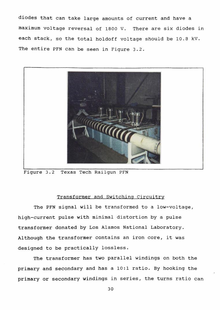
diodes that can take large amounts of current and have a
maximum voltage reversal of 1800 v. There are six diodes in
each stack, so the total holdoff voltage should be 10.8 kV.
The entire PFN can be seen in Figure 3.2.
Figure 3.2 Texas Tech Railgun PFN
Transformer and Switching Circuitry
The PFN signal will be transformed to a low-voltage,
high-current pulse with minimal distortion by a pulse
transformer donated by Los Alamos National Laboratory.
Although the transformer contains an iron core, it was
designed to be practically lossless.
The transformer has two parallel windings on both the
primary and secondary and has a 10:1 ratio. By hooking the
primary or secondary windings 1n series, the turns ratio can
30
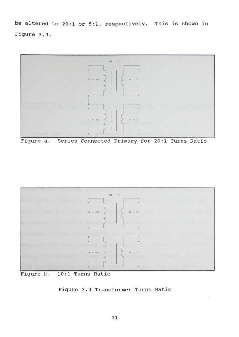
be altered to 20:1 or 5:1, respectively. This is shown in
Figure 3.3.
20
N = 6
N = 6
Figure a. Series Connected Primary for 20:1 Turns Ratio
10
N = 60 N = 6
N = 60 N = 6
Figure b. 10:1 Turns Ratio
Figure 3.3 Transformer Turns Ratio
31
5
N = 60
N - 6
Figure c. Series Connected Secondary for 5:1 Turns Ratio
Figure 3.3 Continued
There are two ways of switching power to the rails.
The fuse of the projectile can trigger the discharge of the
power supply, known as running the rails "hot," or the power
can be delivered to the railgun as the projectile enters the
breech. The first method is simpler, but the second method
insures that voltage breakdown will not occur between the
rails before the gun is fired. Also, the first method is
invalid for our type of power supply. The PFN, which is on
the primary of the transformer, is charged slowly, and the
secondary of the transformer is open circuited. The slow
charge of the PFN acts as a d.c. signal, which would short
through the primary transformer windings. Whereas this
would not harm the charging power supply, the PFN would
never be able to charge to high voltage.
Therefore, in this system, the current is switched to
the rails through a size E ignitron, placed in series with
32

the low-current side, or the primary, of the transformer.
This method requires a sophisticated timing method which
will be discussed in the following section on controls.
Mechanical Design
Designing high energy systems requires careful
consideration of mechanical, as well as electrical, design.
The high current from the transformer to the railgun, as
well as from the PFN to the transformer create forces
comparable to that in the railgun. The difference is that
the railgun has a massive support structure. Another
consideration is the extra inductance inherent in any type
of current feed, be it strip line or coaxial cable. The two
main criteria for design are the strength and support and
lowest possible inductance. Discussed in this section will
be the design of the high-current buswork, the pre-injector
gas gun, and the railgun.
High-Current Buswork
The physical considerations for the Texas Tech railgun
for the high-current buswork were: it had to interface with
the transformer and the railgun, the buswork had to be out
of the way of the main work area of the injector gun, the
current was going to be split symmetrically on each side of
the gun, and it had to be sturdy enough to withstand the
forces generated by the high currents. The electrical
33
considerations were to keep the inductance and resistance to
a minimum.
Two types of buswork considered were coaxial cable and
parallel plates. The advantages of using coaxial cable are
the low inductance, and the transformer connections were
made for large cable, such as RG-19. The inductance for RG-
19 cable is calculated in Equation 3.1
Lcoax = IJ.llo ln b H = 308.09 nH 2 a m m
( 3 .1)
where inner diameter, a= 3/32", and outer diameter,
b = 7/16". However, in a previous experiment with
comparable current [10], the connection from the coax system
to the railgun was compromised during each shot. The coax
cable blew out of the connection, and had to be refitted.
Also, the cable would have to be routinely checked for
defects. If a bad cable went undetected, the other cables
would be forced to carry more current, which would put
additional strain on the system.
The parallel plate system was chosen for the buswork.
Although the inductance was higher than the coax, it was not
excessive. The transformer connections were modified
without major design changes, and the connection to the
railgun was much simpler than for coaxial cables. For
copper with a cross section of 3" x 1/2 11 , the inductance and
resistance is calculated in Equations 3.2 and 3.3
34
Ll d H 439.33 nH = 1-LowKdw = m m
(3.2)
Rl 1 Ohm = a A m
(3.3)
where d = distance between rails, w = width of rails,
A = area of rails, 1 = length of rails, s = conductivity of
copper, and Kdw = 0.6 [11]. Skin effect due to the
frequency of the pulse is taken into consideration for the
resistance value.
The buswork was designed to withstand the force
generated by a 1 MA pulse. If the buswork was not clamped,
the high currents would tend to blow the plates apart. For
symmetry and to reduce the forces, there are two sets of
parallel plates, one on each side of the gun. The force is
proportional to the square of the current; therefore,
halving the current reduces the forces by a factor of four.
For 500 kA, the shearing force on the plates is
8.69(106) N, or 1.95(106
) lbf. Designing for a factor of
safety of 2, 3/4 11 diameter, Grade 8 bolts can withstand a
maximum force of 26,507 lbf. The total number of bolts
needed, which is 74 for each set of plates, is determined by
dividing the total force by the maximum force each bolt can
take.
The bolts cannot be directly connected to the positive
and negative plates. Blocks of insulators wider than the
35
,
buswork plates with aluminum backing will serve as the
medium to connect the bolts. Therefore, the clamp material
must be strong enough to take the pressure exerted by the
bolts. The original choice of material was G-10 because of
its high mechanical strength. However nylon was used
because of its availability, and its strength is sufficient.
The clamps are 6" squares of nylon with aluminum backing,
with six bolts per clamp. There are twelve clamps, spaced
6" apart, for each set of parallel plates.
Pre-Injector Gas Gun
The pre-injector gun and railgun was designed and
fabricated by Dr. Kim Reed, formally of the University of
Texas at Arlington. Several slight modifications were made
at Texas Tech to enhance the operation of the gas gun. The
injector uses highly pressurized gas to accelerate the
projectile. By the time the projectile reaches the breech
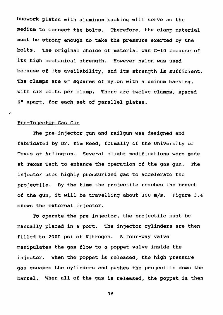
of the gun, it will be travelling about 300 mjs. Figure 3.4
shows the external injector.
To operate the pre-injector, the projectile must be
manually placed in a port. The injector cylinders are then
filled to 2000 psi of Nitrogen. A four-way valve
manipulates the gas flow to a poppet valve inside the
injector. When the poppet is released, the high pressure
gas escapes the cylinders and pushes the projectile down the
barrel. When all of the gas is released, the poppet is then
36
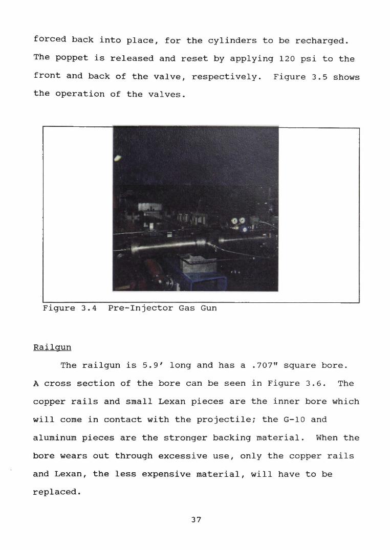
forced back into place, for the cylinders to be recharged.
The poppet is released and reset by applying 120 psi to the
front and back of the valve, respectively. Figure 3.5 shows
the operation of the valves.
Figure 3.4 Pre-Injector Gas Gun
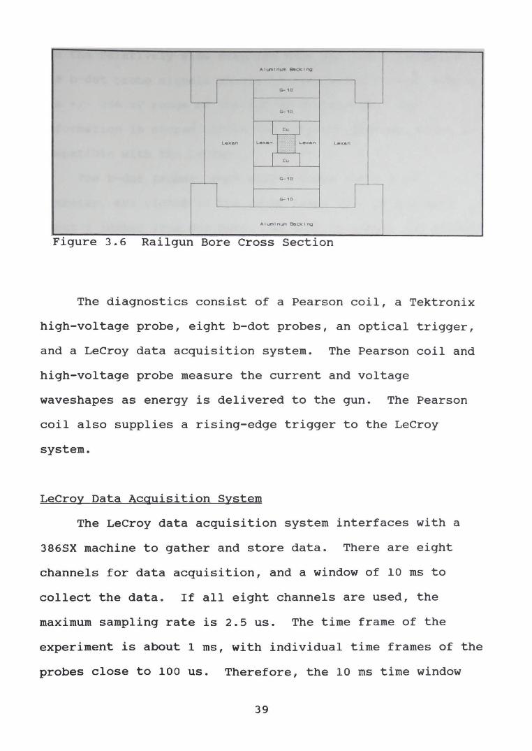
Rail gun
The railgun is 5.9' long and has a .707" square bore.
A cross section of the bore can be seen in Figure 3.6. The
copper rails and small Lexan pieces are the inner bore which
will come in contact with the projectile; the G-10 and
aluminum pieces are the stronger backing material. When the
bore wears out through excessive use, only the copper rails
and Lexan, the less expensive material, will have to be
replaced.
37
hIgh p,..essure
1"111 line
release poppe't. reset:. poppet
120 psi
1"1 1 1 line
Figure 3.5 Pre-Injector Gun Poppet Valve Operation
At the breech end, the bore is modified to make a
smooth connection to the pre-injector gun. Also at the
breech, the copper buswork coming from the power supply is
bolted onto the rails to make a solid electrical connection.
The muzzle end of the bore is attached to a drift tube which
can be elongated. The drift tube is then connected to a
very sturdy catch tank that not only stops the projectile
but also provides a port for the vacuum system.
Controls and Diagnostics
The injector gun and power supply may be manipulated
through a control panel designed and built by another
graduate student, Michael Day. Safety precautions are taken
to be able to abort the operating procedure at any stage and
to prevent any unintentional firing of the gun.
38
A 1 uonl num Qeclc 1 no
G-10
I I- --G- 10
I Cu I Le)(an Lexon I I Le><an lexan
I Cu I G-10
-
G-10 I AIL.6nlnum 91Scklng
. . F1gure 3.6 Ra1lgun Bore Cross Sect1on
The diagnostics consist of a Pearson coil, a Tektronix
high-voltage probe, eight b-dot probes, an optical trigger ,
and a LeCroy data acquisition system. The Pearson coil and
high-voltage probe measure the current and voltage
waveshapes as energy is delivered to the gun. The Pearson
coil also supplies a rising-edge trigger to the LeCroy
system.
LeCroy Data Acquisition System
The LeCroy data acquisition system interfaces with a
386SX machine to gather and store data. There are eight
channels for data acquisition, and a window of 10 ms to
collect the data. If all eight channels are used, the
maximum sampling rate is 2.5 us. The time frame of the
experiment is about 1 ms, with individual time frames of the
probes close to 100 us. Therefore, the 10 ms time window
39
and the relatively slow sampling rate are not a hindrance.
The b-dot probe signals should be attenuated to stay within
the +/- 256 mv range of the LeCroy digitizers. The
information is stored within the catalyst program, which is
compatible with the LeCroy.
The b-dot probes, each with 8 turns and a 3 mm
diameter, are placed in the outer Lexan wall of the gun,
about 4 inches from the bore. At this distance, the maximum
magnetic field intensity should be about 1 Tesla for a 500
kA shot. Assuming the risetime of the pulse to be less than
100 us, the probe voltage should be less than 1 V, according
to Equation 2.19.
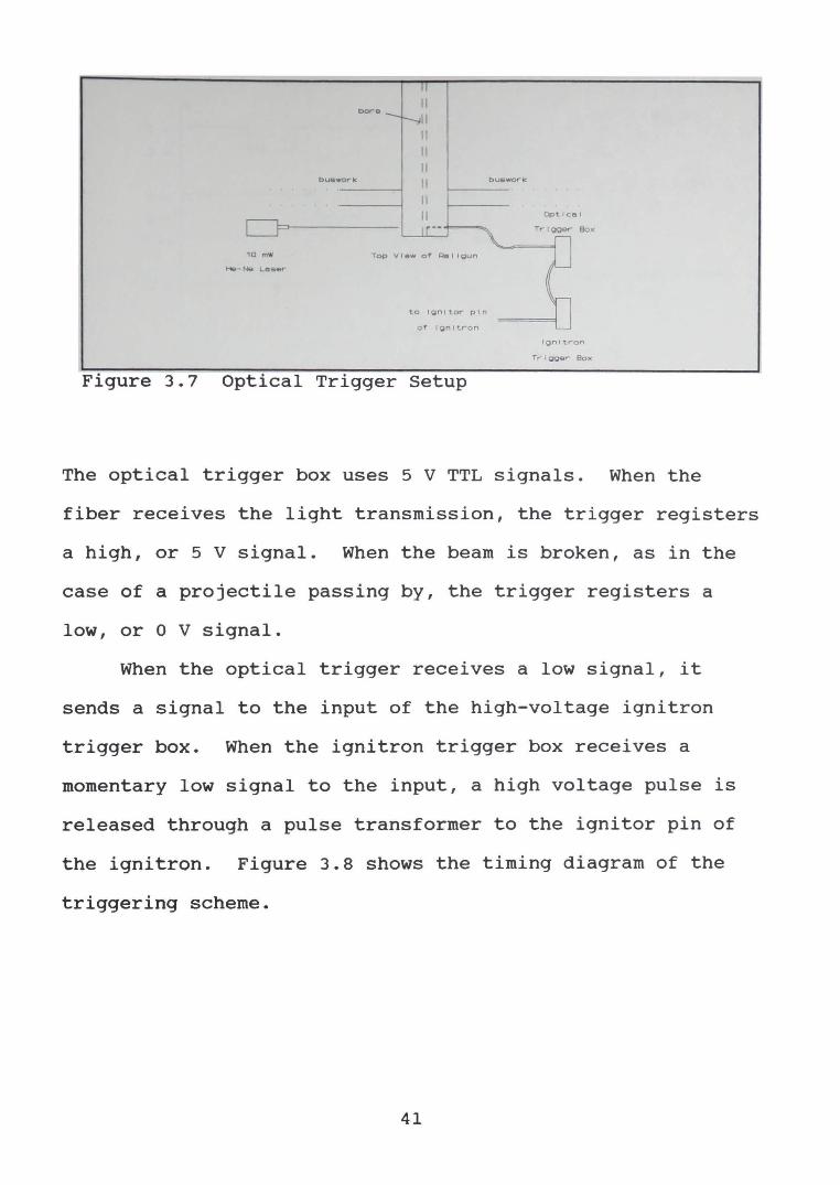
Optical Trigger for Ignitron
The purpose of the optical trigger is to have the
projectile and the current reach the breech of the railgun
at approximately the same time. The optical trigger sends
an input signal to a high-voltage trigger box, which fires
the ignitron. Constructed by Michael Day, the optical
trigger fires the ignitron when the projectile exits the
preinjector gun. Optical sensors are ideal for this
experiment because they are unaffected by the noisy
environment of the railgun.
A 10 mW He-Ne laser is aligned across the bore with an
optical fiber where the gas gun connects with the railgun,
as shown in Figure 3.7.
40
II
II bor-e -
~II II II II
buaworle II bU&'NOrk:
II II Opt leo!
0=---- 1r·· - TriQQer'" BoK
10 mW Top V lew of Re 1 I gun
He-Ne Lo&er-
to Ignitor pin
Of lgn 1 t.ron
tgnl't.ron
Trigger- Box . F1gure 3.7 Opt1cal Tr1gger Setup
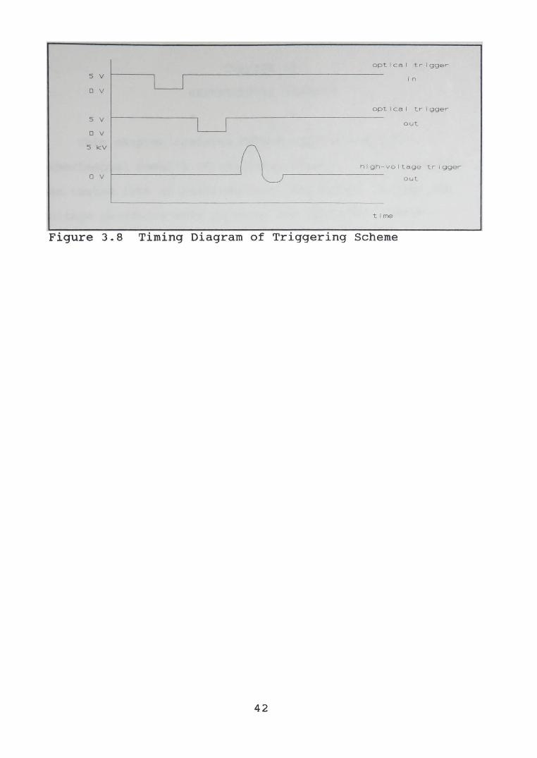
The optical trigger box uses 5 V TTL signals. When the
fiber receives the light transmission, the trigger registers
a high, or 5 V signal. When the beam is broken, as in the
case of a projectile passing by, the trigger registers a
low, or o V signal.
When the optical trigger receives a low signal , it
sends a signal to the input of the high-voltage ignitron
trigger box. When the ignitron trigger box receives a
momentary low signal to the input, a high voltage pulse is
released through a pulse transformer to the ignitor pin of
the ignitron. Figure 3.8 shows the timing diagram of the
triggering scheme.
41
optic~ I trigger
5 v I I in
0 v
optical trigger
5 v I I out
0 v
5 kV
high- voltage trigger 0 v out
tlme
Figure 3.8 Timing Diagram of Triggering Scheme
42
CHAPTER IV
EXPERIMENTAL RESULTS
This chapter contains PSPICE simulations and
experimental results of the power supply. First, the PFN
was tested into an ignitron load, and output current and
voltage waveforms were obtained for different charging
voltages. Also, the current in each capacitor and diode
were measured at low charging voltages. Next, the PFN was
fired directly into the railgun at low voltages, and current
data was obtained. The pulse transformer was modelled in
PSPICE, and the performance was tested into a short circuit
load. once the PFN and pulse transformer were tested
separately, they were tested together into the railgun.
Velocity, as well as current and breech voltage measurements
were taken for a PFN charge voltage of 5 kV.
PFN Testing
PFN Into an Ignitron Load
To determine current waveforms of each stage, the PFN
was discharged into an ignitron load at different charging
voltages. When the switch closes, the impedance is
basically a short circuit. Although the railgun load is
more complex and dynamic, the ignitron results give an
approximation of the final current waveform into the
43
railgun. The impedance of the Size E ignitron used is .003
Ohm [11].
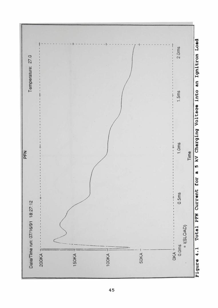
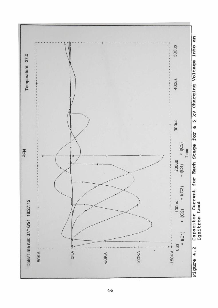
The following PSPICE results in Figures 4.1 through 4.4
are for individual currents in each capacitor, inductor, and
diode, plus the total current. The PSPICE listing for the
following results is in Appendix A. The initial spike is a
switching transient that disappears when the load is
modelled as a resistor instead of a switch. Also, the spike
does not appear in any of the experimental results.
The experimental results in Figures 4.5 through 4.12
are capacitor and diode currents for a 1 kV charging
voltage. Although the charging voltage differs from the
PSPICE results, the waveshape can be compared to the
simulations. The experimental results throughout this
chapter are shown in the form of an oscilloscope trace. In
some of the pictures, the reference line, where the trace
started, is not inherently obvious. To reduce confusion on
the reader's part, the reference line will be noted on each
of the oscilloscope traces.
44
~
U1
PF
N
Dat
eiT
ime
run:
07/
16/9
1 18
:27:
12
Tem
pera
ture
: 27
.0
20
0K
A l.
--· ---
---· · -
--· + --
---
· · -
---
---·
-·
+-
--
--
--
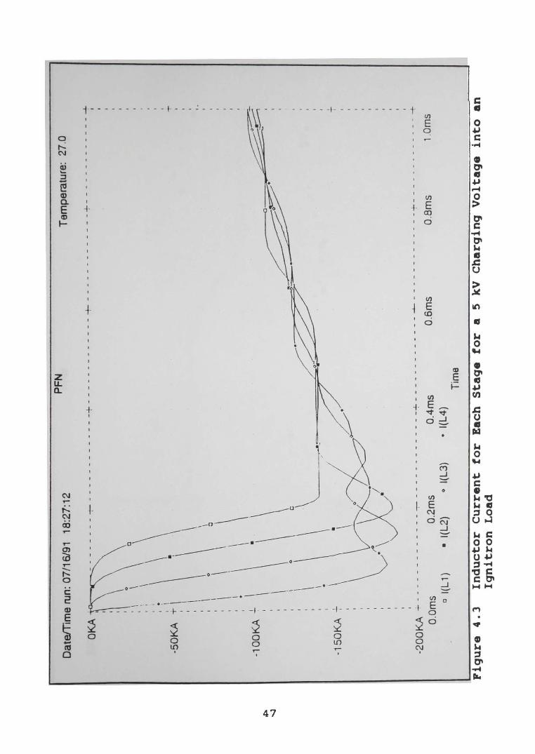
--
--
· -
--
-· ~ -
· ·
--
· -
· ·
· ·
· -
--·1
110
: II!\
~
. 15
0KA
~ !
~ +
I I I I
10
0K
A +
l I I
! 5
0K
A 7
I !
J
..!..
OK
A +
---
----
----
----
--~-
----
----
----
----
+-
--
--
--
--
--
--
--
--~ -
--
--
--
--
--
--
--
-~
O.O
ms
O.S
ms
1.0
ms
1.5
ms
2.0
ms
D
I(S
LO
AD
) Ti
me
Fig
ure 4~1
To
tal
PFN
cu
rren
t to
r a
5 kV
C
ha
rqin
q V
olt
ag
e in
to
an
Iq
nit
ro
n
Loa
d
~
0'1
PF
N
Tem
pera
ture
: 27
.0
Dat
e/T
ime
run:
07/
16/9
1 18
:27
:12
SOK
A -
--
--
--
--
--
--
-+
---
----
----
--+
--
--
--
--
--
--
-~ -
--
--
--
--
--
--+
--
--
--
--
--
--
--+
I
I
. r
.
~~·~
OKA~·-~•
I /"
a:::
:::::
-I
o
I I I I
-50
KA
i ' ' v I I I ! v
-10
0K
A T
., i
I -I
I \ I
\
I )(
• i ~
----
1=--
----
r"
'0
.... 0
o.., <
~·
r I
~
0 r
~
\.
0
I I
I I
• I
i I
) 0
\/
.. ,..
...__......
.
\j
0
' T
-15
0K
A +
_!---
--
--
--
--
-~ -
--
--
--
--
--
--+
--
--
--
--
--
--
-~ -
--
--
--
--
--
--T
--
--
--
--
--
--
-~
Ous
· 10
0us
200u
s 30
0us
400u
s 50
0us
a l(
C1)
•
l(C
2)
o I(
C3
) •
l(C4)
•
l(CS
) T
ime
Fiq
ure
4
.2
Cap
acit
or
Cu
rren
t fo
r E
ach
Sta
ge fo
r a
5 kV
Ch
arg
ing
Vo
ltag
e in
to a
n
Ign
itro
n L
oad
~
I "'-
l
Dat
e/T
ime
run:
07/
16/9
1 18
:27:
12
PF
N
Tem
pera
ture
: 27
.0
OK
A ~ -
--
--
--
--
--
--
--
--
--
---
1-
--
--
--
--
--
--
-~ -
--
--
--
--
--
--
-~.. -
--
--
--
--
--
--
...-~..
I· •
' ,
' I
-50
KA
I ~ +\
: I
I \
0 \ \ \
~
I \
I . 1
,\
~~
: l
\ . -~
; \
\ ,
• ~
-10
0K
A l
. I
I \ \ i
0
\
\ ~?-/
· \
0 "---
.
I '
. -1
50
KA
7
i
I •
I
-20
0K
A ~ -
--
--
--
--
--
--
....-
--
--
--
--
--
--
-+-
--
--
--
--
--
--
...._ -
--
--
--
--
--
--+
--
--
--
--
--
--
--+
O.O
ms
0.2
ms
0.4
ms
0.6
ms
0.8
ms
1.0m
s a
I(L
1)
• I(
L2)
o l(
L3
) •
I(L4
) Ti
me
Fig
ure
4
.3
Ind
ucto
r cu
rren
t fo
r E
ach
stag
e fo
r a
5 kV
C
har
gin
g V
olt
age
into
an
Ig
nit
ron
Loa
d
,c:.
00
Da
te/T
ime
run
: 07
/16/
91
18
:27
:12
P
FN
Tem
pera
ture
: 27
.0
20
0K
A +
--
--
--
--
--
--
--+-
----
----
----
--+
--
--
--
--
--
--
--+
----
----
----
--7
--
--
--
--
--
--
--+
I
I
I
15
0K
A ~
10
0K
A -
7-
I S
OK
A 7
•
I Q I 0
: ~
~
....
----
----
----
----
----
--0-
----
---
0~
: Jl
• I
. .
I ~
0 JG\
~-H l i
Jl. \I
~>> .
. .
. -~
=-··-
H~ -O
KA
O
.Om
s 0
.2m
s 0
.4m
s 0
.6m
s O
.Bm
s 1.
0ms
c 1(
01)
• 1(
02)
0 1(
03)
• 1(
04)
9 1(
05)
Tim
e
Fig
ure
•·•
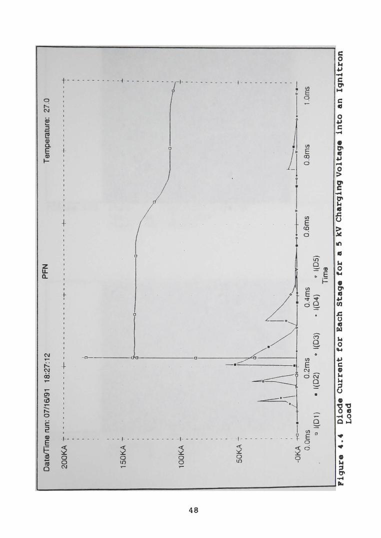
D
iod
e cu
rren
t to
r E
ach
Sta
ge
for
a 5
kV C
har
gin
g V
olt
ag
e in
to a
n
Ign
itro
n
Loa
d
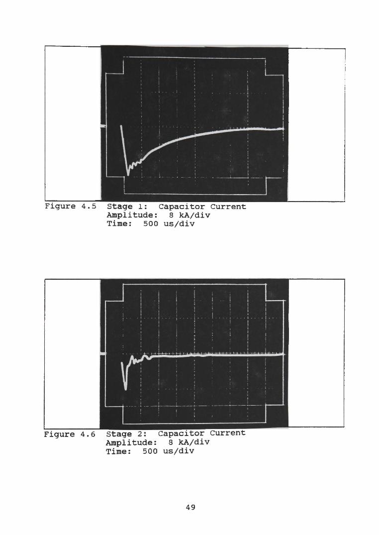
Figure 4.5 stage 1: capacitor current Amplitude: 8 kA/div Time: 500 usjdiv
Figure 4.6 Stage Amplitude: Time: 500
49
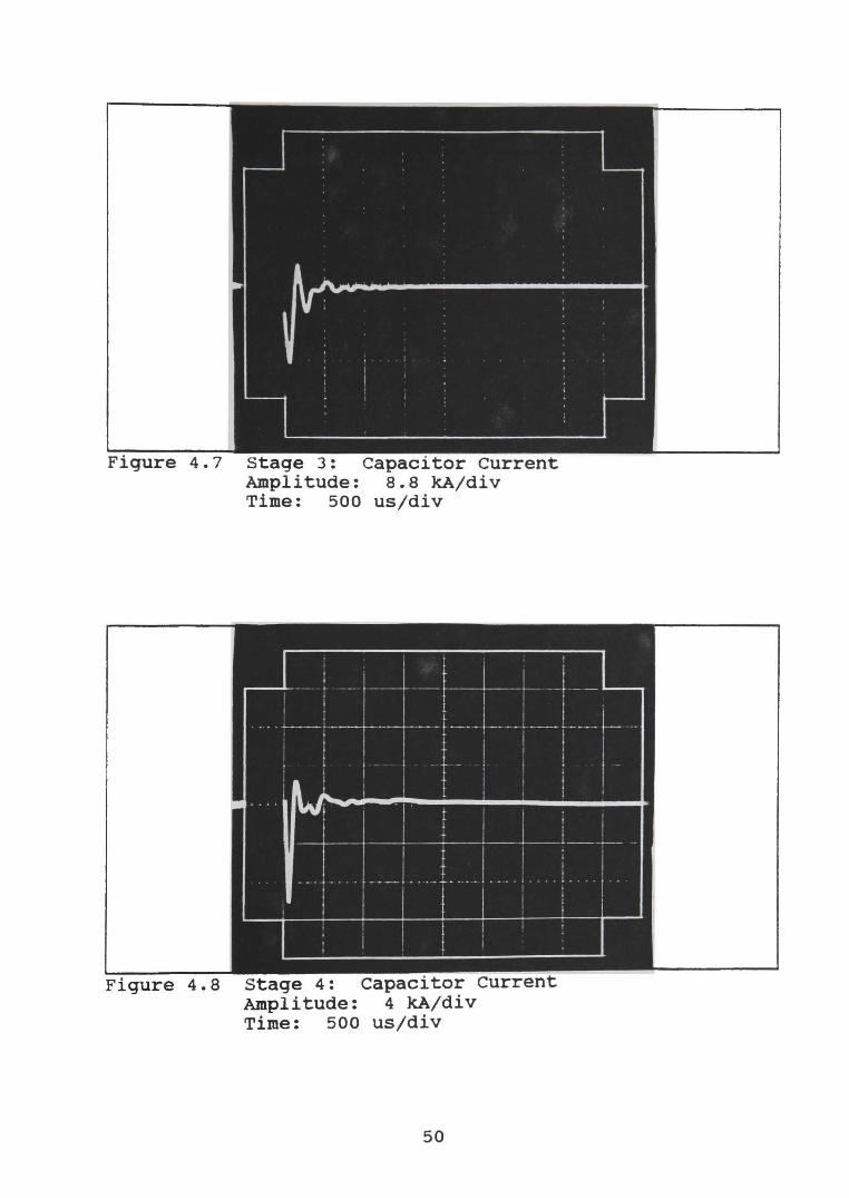
Figure 4.7 stage 3: capacitor current Amplitude: 8.8 kA/div Time: 500 us/div
Figure 4.8 stage 4: capacitor current Amplitude: 4 kA/div Time: 500 usjdiv
50
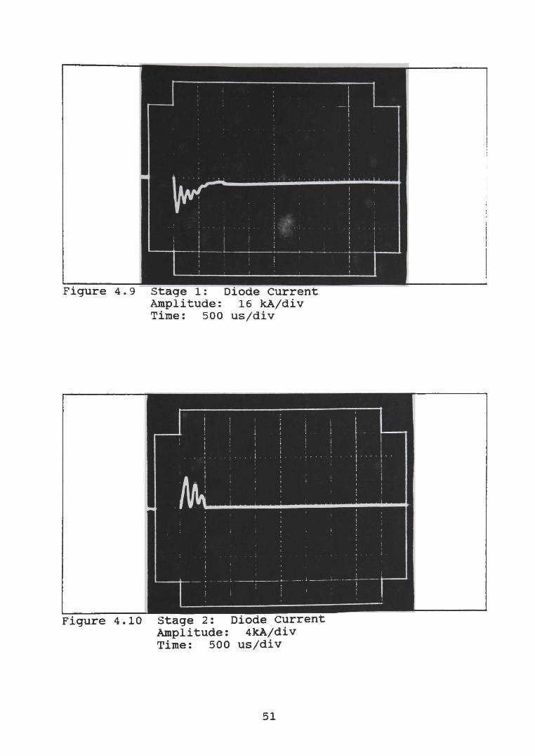
Figure 4.9 Stage 1: Diode Current Amplitude: 16 kA/div Time: 500 us/div
Figure 4.10 current Amplitude: 4kA/div Time: 500 us/div
51
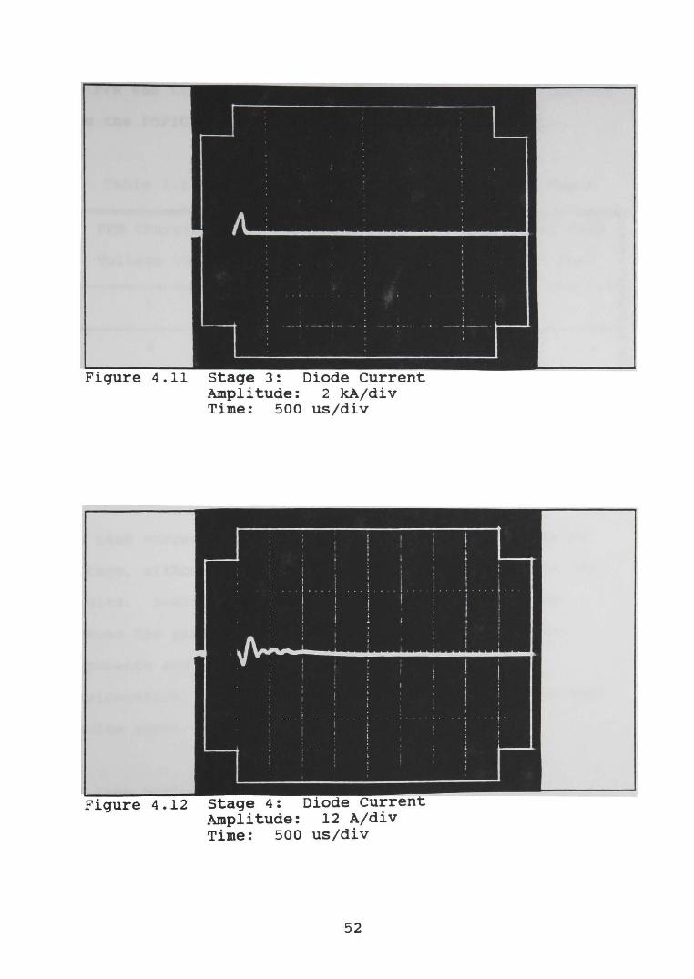
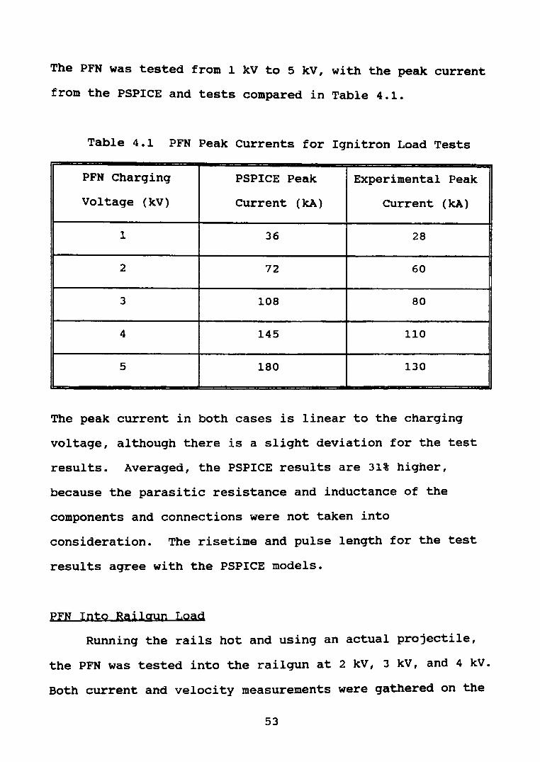
Figure 4.11 stage 3: Diode current Amplitude: 2 kA/div Time: 500 usjdiv
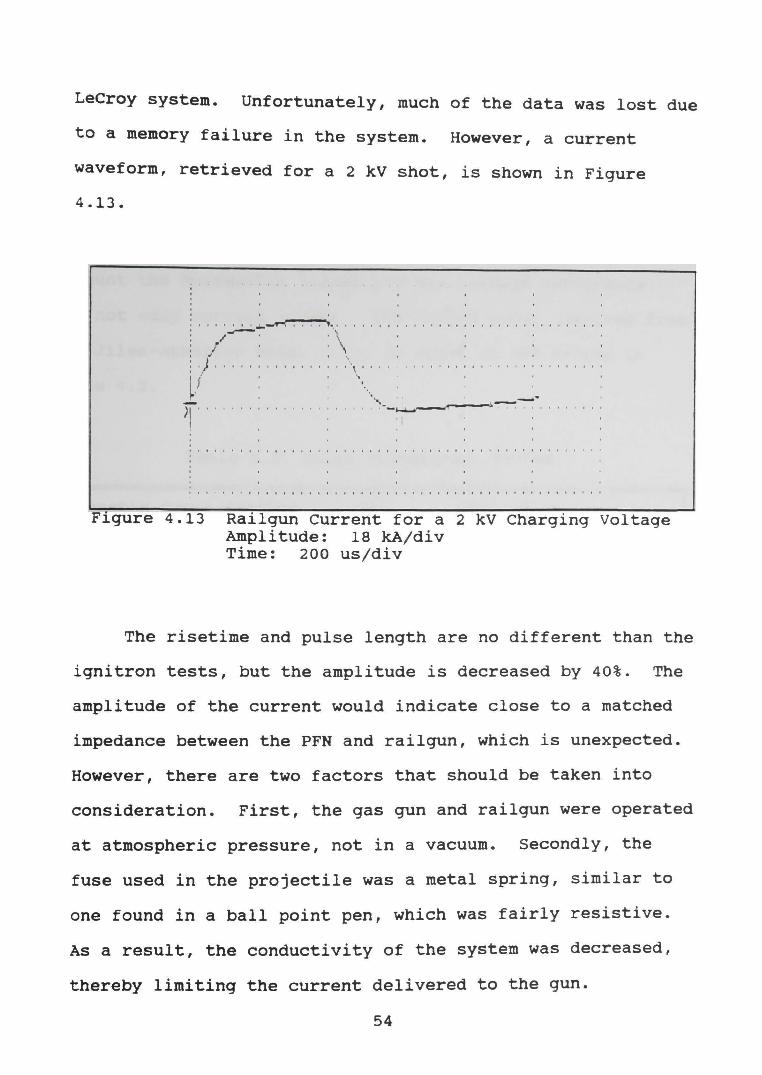
Figure 4.12 current Amplitude: 12 A/div Time: 500 usjdiv
52
The PFN was tested from 1 kV to 5 kV, with the peak current
from the PSPICE and tests compared in Table 4.1.
Table 4.1 PFN Peak Currents for Ignitron Load Tests
PFN Charging PSPICE Peak Experimental Peak
Voltage (kV) Current (kA) Current (kA)
1 36 28
2 72 60
3 108 80
4 145 110
5 180 130
The peak current in both cases is linear to the charging
voltage, although there is a slight deviation for the test
results. Averaged, the PSPICE results are 31% higher,
because the parasitic resistance and inductance of the
components and connections were not taken into
consideration. The risetime and pulse length for the test
results agree with the PSPICE models.
PFN Into Railgun Load
Running the rails hot and using an actual projectile,
the PFN was tested into the railgun at 2 kV, 3 kV, and 4 kV.
Both current and velocity measurements were gathered on the
53
LeCroy system. Unfortunately, much of the data was lost due
to a memory failure in the system. However, a current
waveform, retrieved for a 2 kV shot, is shown in Figure
4.13.
' ' ' ;~~~ ' ' ' ' :··\' ' ' ' ' ' ' : ' ' ' ' ' ' ' : ' ' ' ' ' ' ' : ' ' ' ' ' ' ' : I , ,
·)J ·'' '':' '' '' '':' .'\''' ' '' ''' ' '':' ' ' '' '' : ''' '' '':
~f ' ' .. . ' ' '
' ·, ' ' · ... , , ' ~· ' - ... -~.-)1' '''' ''''' ''''''''' '' .--~ ~· . '' '''' '' ' ' '.
1 t I • ' I I
0 1 1 o 0 I I
I I I I I ' I I I I It I I I I I I I I I I I I I 0 I I It It I I I I I I It It I I It I I'
I I t I I I 0 I I I I I I I I 0 I I I I I t I I I I It I I I I If I I I I 0 I I I I I I
Figure 4.13 Railgun Current for a 2 kV Charging Voltage Amplitude: 18 kA/div Time: 200 us/div
The risetime and pulse length are no different than the
ignitron tests, but the amplitude is decreased by 40%. The
amplitude of the current would indicate close to a matched
impedance between the PFN and railgun, which is unexpected.
However, there are two factors that should be taken into
consideration. First, the gas gun and railgun were operated
at atmospheric pressure, not in a vacuum. Secondly, the
fuse used in the projectile was a metal spring, similar to
one found in a ball point pen, which was fairly resistive.
As a result, the conductivity of the system was decreased,
thereby limiting the current delivered to the gun.
54
Pulse Transformer Testing
Pulse Transformer Model
If the magnetic core dimensions of the transformer and
the number of turns of the primary and secondary are known,
a reasonably accurate model can be simulated on the
professional version of PSPICE. The model takes into
account the hysteresis losses and the leakage inductance,
but not eddy current losses. The PSPICE model, derived from
the Jiles-Atherton model [12], is based on the values in
Table 4.2.
Table 4.2 Pulse Transformer Values
Magnetic Cross-Section 1206.45 em
Magnetic Path Length 279.4 em
Air Gap Length .OS em
Magnetization Saturation 600 A/m
Coupling Coefficient 99 %
Primary Resistance 8.58 mOhm
Secondary Resistance 1.72 mOhm
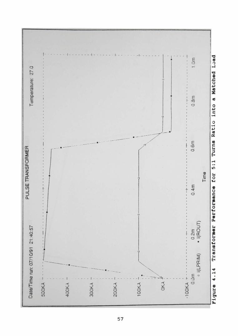
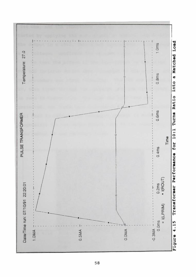
The results are shown in Figure 4.14 and Figure 4.15.
The PSPICE listings for each case are placed in the
appendix. In the first two simulations, a 100 kA PFN
55
waveform is pulsed through the transformer into a low
impedance load, representing a matched case for the PFN.
The runs are made for a 5:1 and 10:1 turns ratio,
respectively. The rise and fall times are unaffected, and
the transformer does not saturate. However, there is a 7%
droop for the 500 kA shot and a 25% droop for the 1 MA shot.
Although the performance drops drastically for the 1 MA
pulse, the pulse shape will not be compromised severely for
the 500 kA pulse.
In Figures 4.16 through 4.21, the PFN, with an initial
charge voltage of 5 kV, supplies the current pulse. The
following runs test the transformer into a variety of loads
to see the effect of the railgun and buswork impedance.
These results will be presented in the following section on
high-current testing into the railgun.
Pulse Transformer Tests
The transformer turns ratio and magnetizing inductance
was tested with 120 V a.c •• To test the magnetizing
inductance, the a.c. wall plug was hooked directly to the
primary of the transformer, with the secondary open
circuited. The a.c. impedance of an inductor is
Za.c. = 2Tif L Ohm (4.1)
where f=60 Hz. The circuit drew .5 A, so the impedance was
56
U1
-....J
Da
te/T
ime
run
: 07
/10/
91
21:4
0:5
7
PU
LS
E T
RA
NS
FO
RM
ER
T
em
pe
ratu
re:
27.0
--
--
--~
--
--
--
--
--
--
--
--
--
-7
--
-~
--
--
--
--
--
--
--
--
--
--
----
--
--
--
--
--
--
-
i I 50
CK
A
400K
A -
30
0K
A -
20
0K
A ~
I
10
0K
A
I • I
I :/ 0
j:
KA
:
I I I I I • j
I I • I I I / ~
• I ' \ 1: I I \ I ' \ • . I \ i ' • \
"':..
\
-!..
~
',~
' \ ~
., __
__
__ _
-1 00
KA
+ -
--
--
--
--
--
--
+-
--
--
--
--
---
--+
---
----
---
---.
...,...--
---
----
--
---
-:--
----
----
---
--O
.Om
0
.2m
0
.4m
0
.6m
O
.Bm
1
.0m
c
I(LP
RIM
) •
!(R
OU
T)
Tim
e
Fiq
ure
4
.14
T
ran
afo
raer
Perf
ora
an
ce
for
5:1
T
urn
s R
ati
o
into
a
Matc
hed
L
vad
VI
(X)
Da
tetT
ime
run
: 07
/10/
91
22:2
0:01
P
UL
SE
TR
AN
SF
OR
ME
R
Tem
pera
ture
: 27
.0
1.0
MA
-
--
--
--
--
--
--
--7
--
--
--
--
--
--
---
:---
--
--
--
--
--
--~ -
--
--
--
--
--
----
--
--
--
--
--
--
;
I I ~-------------
• I ~ \ i
I \ • \
0.5
MA
1
• I
I T
•
O.O
MA
vo
o--
-o-~
\
I \
w--
-·
\ I
L. ---
----
----
----
·----------~
-0.3
MA
--------------
-r-------------
--:---
---
---------~------------
------
---
---
--
O.O
ms
0.2
ms
0.4m
s 0
.6m
s 0
.8m
s 1
.0m
s
c l(
LP
RIM
) •
I(R
OU
T)
n~
-I-
·riq
ure
4.1
5
Tra
net
ora
er
Per
fora
an
ce to
r 1
0:1
T
urn
e R
ati
o
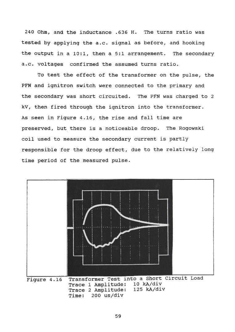
into
a
Ha
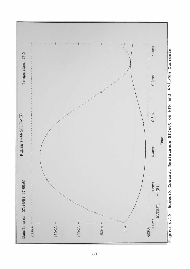
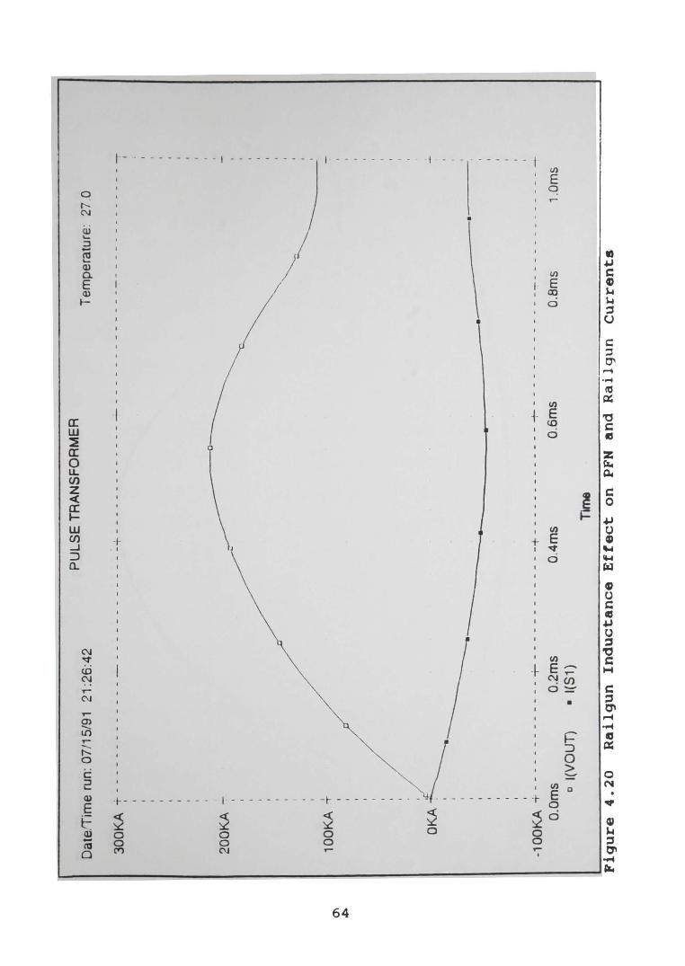
tch
ed
Loa
d
240 Ohm, and the inductance .636 H. The turns ratio was
tested by applying the a.c. signal as before, and hooking
the output in a 10:1, then a 5:1 arrangement. The secondary
a.c. voltages confirmed the assumed turns ratio.
To test the effect of the transformer on the pulse, the
PFN and ignitron switch were connected to the primary and
the secondary was short circuited. The PFN was charged to 2
kV, then fired through the ignitron into the transformer.
As seen in Figure 4.16, the rise and fall time are
preserved, but there is a noticeable droop. The Rogowski
coil used to measure the secondary current is partly
responsible for the droop effect, due to the relatively long
time period of the measured pulse.
Figure 4.16 Transformer Test into a Short Circuit Load Trace 1 Amplitude: 10 kA/div Trace 2 Amplitude: 125 kA/div Time: 200 usjdiv
59
The short circuit connections actually had an impedance
of about .005 Ohm, which is .5 Ohm reflected to the primary.
The larger load impedance smoothes the waveform and
decreases the PFN current amplitude. The maximum PFN
current is 25 kA, and the secondary current, with a 10:1
turns ratio, is approximately 250 kA.
High-Current Testing Into the Railgun
High-current shots were taken on the railgun to gather
rail current, breech voltage, and projectile velocity
measurements. The PFN was charged to 2 kV and to 5 kV, and
the transformer ratio was 5:1 for every shot. Due to
problems with the optical trigger, the timing of the
ignitron trigger was not accurate, so the pre-injector gun
was bypassed. A copper fuse and an actual projectile were
fired separately. Firing a projectile with no initial
velocity is highly detrimental to the lifetime of the rails.
Therefore, this method will be used only until the optical
trigger can be fixed.
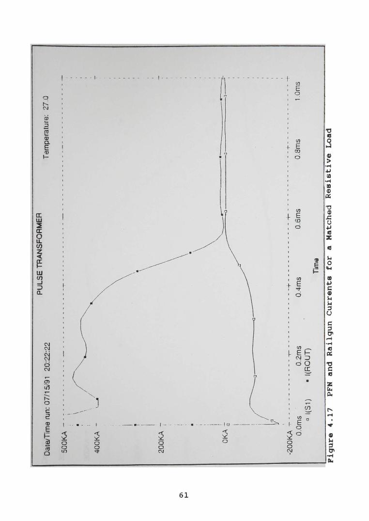
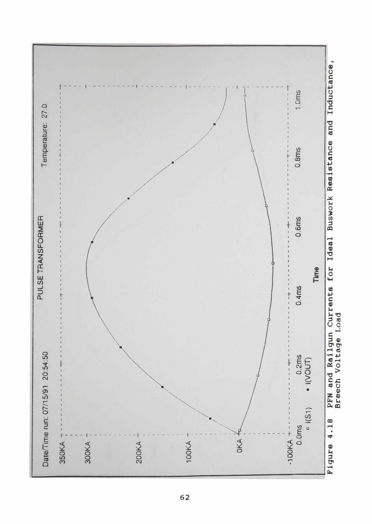
The remainder of the PSPICE results will be presented
in Figures 4.17 through 4.21 and compared to actual data.
The buswork and railgun values are determined, in part, by
actual data taken. In each of the following figures, the
total PFN current is displayed as I(S1) and the total
railgun current as I(ROUT) or I(VOUT).
60
0'1
1-'
PU
LSE
TR
AN
SFO
RM
ER
D
ateJ
Tim
e ru
n: 0
7/15
i91
20:2
2:22
T
em
pe
ratu
re:
27.0
SOO
KA
-
--
---
--
----
--
--
--
---
--
--
---
---
--
--
--
---
--
--
--
--
--
--
--
---
--
--
--
--
--
--·-
-
•
40
0K
A -
i • ! I I 2
00
KA
-:- '
I \ \ \
~ I
..,..
•
• •
OKAl
\_
•
~
i ~
1~
1;--
---,~~
~a -2
00K
A .
.,.. -
--
--
--
--
--
--
-r-
--
--
--
--
--
--
-+-
--
--
--
--
--
--
+
--
--
--
--
--
--
-T-
--
--
--
--
--
--~
O.O
ms
0.2
ms
0.4m
s 0
.6m
s 0
.8m
s 1.
0m
s a
I(S 1
) •
l(R
OU
T)
Tim
e
Fig
ure
4.1
7
PFN
a
nd
R
ail
gu
n
Cu
rren
ts
for
a M
atc
hed
R
esis
tiv
e
Loa
d
0\
l\)
Da
te/T
ime
run
: 07
/15/
91
20:5
4:50
PU
LSE
TRA
NSF
OR
MER
T
empe
ratu
re:
27.0
350K
A "
'7
--
--
--
--
--
--
-~
--
--
--
--
--
--
-+ -
--
--
--
--
--
--~ -
--
--
--
--
--
----
__
__
__
__
__
__
_ I
I
300K
A ~
200K
A _
.:_
100M~
I • I I
'/
OKA
~. '\
. "'-.
... '
~
~c:~ I
-1 O
OKA
+ -
--
--
--
--
---
-+-
--
--
--
--
--
---+
---
----
--
--
---+
--
--
--
--
--
--
--+
--
--
--
--
--
--
-~
O.O
ms
0.2
ms
0.4m
s 0
.6m
s O
.Bm
s 1.
0m
s o
1(51
) •
I(VO
UT)
T
lme
Fig
ure
4
.18
PF
N
an
d
Rail
gu
n C
urr
en
ts
for
Ideal
Bu
swo
rk R
esis
tan
ce
an
d
Ind
ucta
nce,
Bre
ech
V
olt
ag
e
Lo
ad
II 0
\ w
Dat
etT
ime
run:
07/
16/9
1 17
:55:
59
PU
LSE
TR
AN
SF
OR
ME
R
Te
mp
era
ture
: 27
.0
200K
A
--
--
--
--
--
--
--
--
--
--
--
--
--
---
--
--
--
--
--
--
--
--
--
--
--
--
-----
--
--
--
--
--
--
-
15uK
A -
10
0K
A -
5u
KA
- I I
,;
,- I I
aKA~
I I I I
~~ """""
"' \, \
i \ \\
'\ \ -~
-5C
KA
-
--
--
--
--
--
--
--
--
--
--
--
--
---~ -
--
--
--
--
--
--~ -
--
__
__
__
__
__
__
__
__
__
__
__
__
_
O.O
ms
0.2m
s 0.
4ms
0.6
ms
0.8
ms
1.0m
s c
I(V
OU
I)
• 1(
51)
Tim
e
Fig
ure
4
.19
B
usw
ork
C
on
tact
Resis
tan
ce
Eff
ect
on
PF
N
and
R
ail
gu
n C
urr
en
ts
0'1 ~
PU
LS
E T
RA
NS
FO
RM
ER
D
ate
.'Tim
e r
un: 0
7/1
5/91
21
:26
:42
T
em
pe
ratu
re:
27.0
30
0K
A +
--
---
--
---
--
---
--
--
--
--
---
-+ -
--
--
--
--
--
--~ -
--
--
--
--
--
---
--
--
--
--
--
--
-;
I
20
0K
A -
~:
10
0K
A +
OKA~
: ----
--------
------
1
~--------~--------
-· -1
OO
KA
+
--
----
---
----
-+-
--
--
--
--
--
--
-+ -
----
---
--
--
-~ -
--
--
--
--
--
---
--
--
--
----
--
--
O.O
ms
0.2
ms
0.4
ms
0.6
ms
O.B
ms
1.0m
s o
I(V
OU
T)
• I(
S1)
T
ime
Fig
ure
4
.20
R
ail
gu
n
Ind
ucta
nce
Eff
ect
on
PF
N
and
R
ail
gu
n
Cu
rren
ts
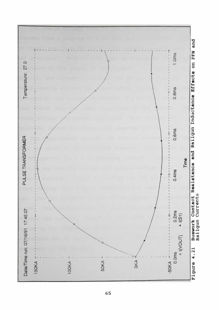
0\
U'l
Da
te/T
ime
run
: 0
7/1
6/9
1
17:4
5:0
7 PU
LSE
TRA
NSF
ORM
ER
Te
mp
era
ture
: 27
.0
15
0K
A ~ -
--
--
--
--
--
--~ -
--~~-
--
--
--
--
--
--
--
--
--
--
--
--
--
i
10
0K
A -
, a
SO
KA
-I :;
OK
A
I I
1/
::J
-
~
--·
I --5
0K
A ~ -
--
--
--
--
--
--
-+---
----
---
----
+ -
----
--
--
----
+ -
---
---
--
---
-+-
--
--
--
--
--
--
-+
O.O
ms
0.2m
s 0.
4ms
0.6
ms
O.B
ms
1.0
ms
o l(V
OU
T)
• I(
S1)
T
ime
Fig
ure
4
.21
B
usw
ork
C
on
tact
Resi
stan
ce
and
R
ail
gu
n I
nd
ucta
nce E
ffects
on
PF
N an
d~
Rail
gu
n C
urr
en
ts
The breech voltage used in the PSPICE listings is
obtained from a picture of 5 kV shot using the copper fuse.
The actual amplitude of the railgun current is much less
than predicted. Much of this loss is attributed to contact
resistance in the joints of the buswork. In Figures 4.19
and 4.21, the contact resistance was chosen so that the
PSPICE results matched the experimental results. To match
the results, the contact resistance is .002 Ohm, which is 20
times higher than the ideal resistance of the buswork. The
breech voltage and system inductance lower the current
amplitude, smooth the pulse, and lengthen the fall time.
The experimental current and voltage waveforms for fuse
shots are shown in the following figures. Figure 4.22 is
the PFN current for a 2 kV charging current. Figures 4.23
and 4.24 are the PFN current and breech voltage for a 5 kV
charging current. Figure 4.25 shows the PFN current and
breech voltage when a Lexan projectile was used with a wider
fuse. For the projectile, the system current is increased
by 20%. This suggests that using an even wider fuse will
increase the current. Obviously, the width of the fuse is
limited by the dimensions of the bore. Further results were
not pursued due to the difficulty of loading the fuse into
the breech of the railgun.
66
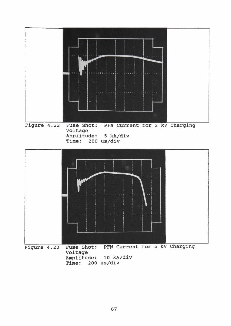
Figure 4.22
Figure 4.23
Fuse Shot: Voltage Amplitude: Time: 200
Fuse Shot: Voltage Amplitude: Time: 200
PFN current for 2 kV Charging
5 k.A/div US/diV
PFN current for 5 kV Charging
10 kA/div US/div
67
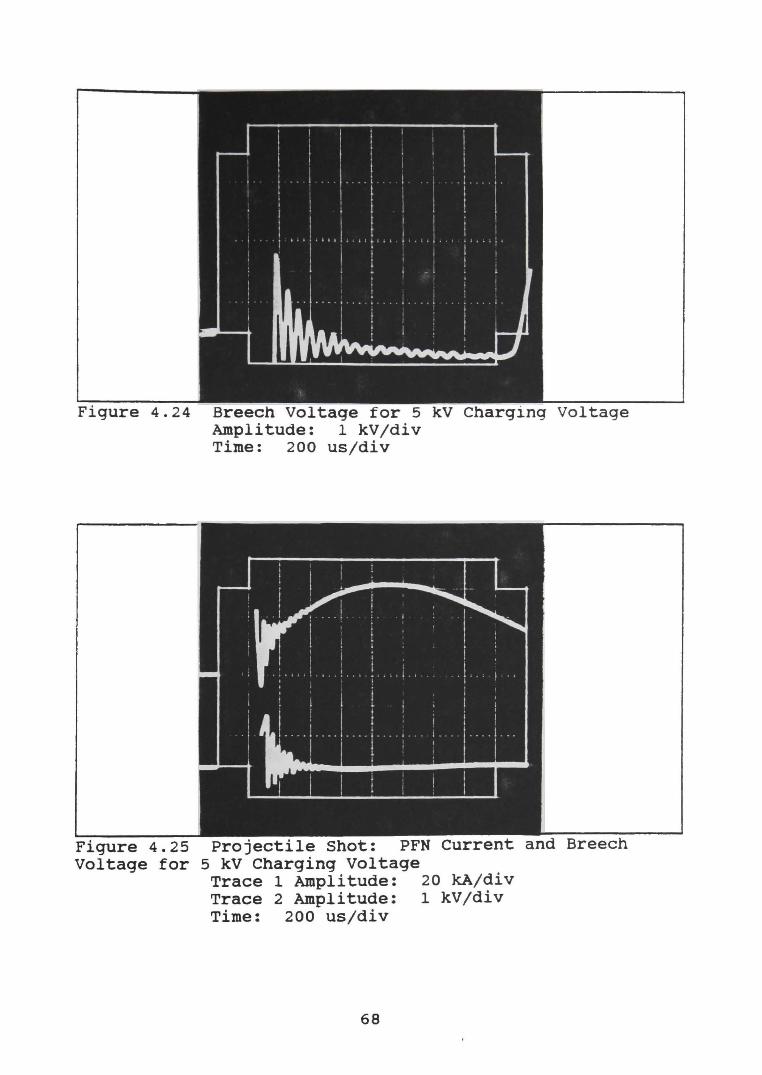
Figure 4.24
Figure 4.25 Voltage for
Breech Voltage for 5 kV Charging Voltage Amplitude: 1 kV/div Time: 200 usjdiv
Projectile Shot: PFN current 5 kV Charging Voltage Trace 1 Amplitude: 20 kA/div Trace 2 Amplitude: 1 kV/div Time: 200 usjdiv
68
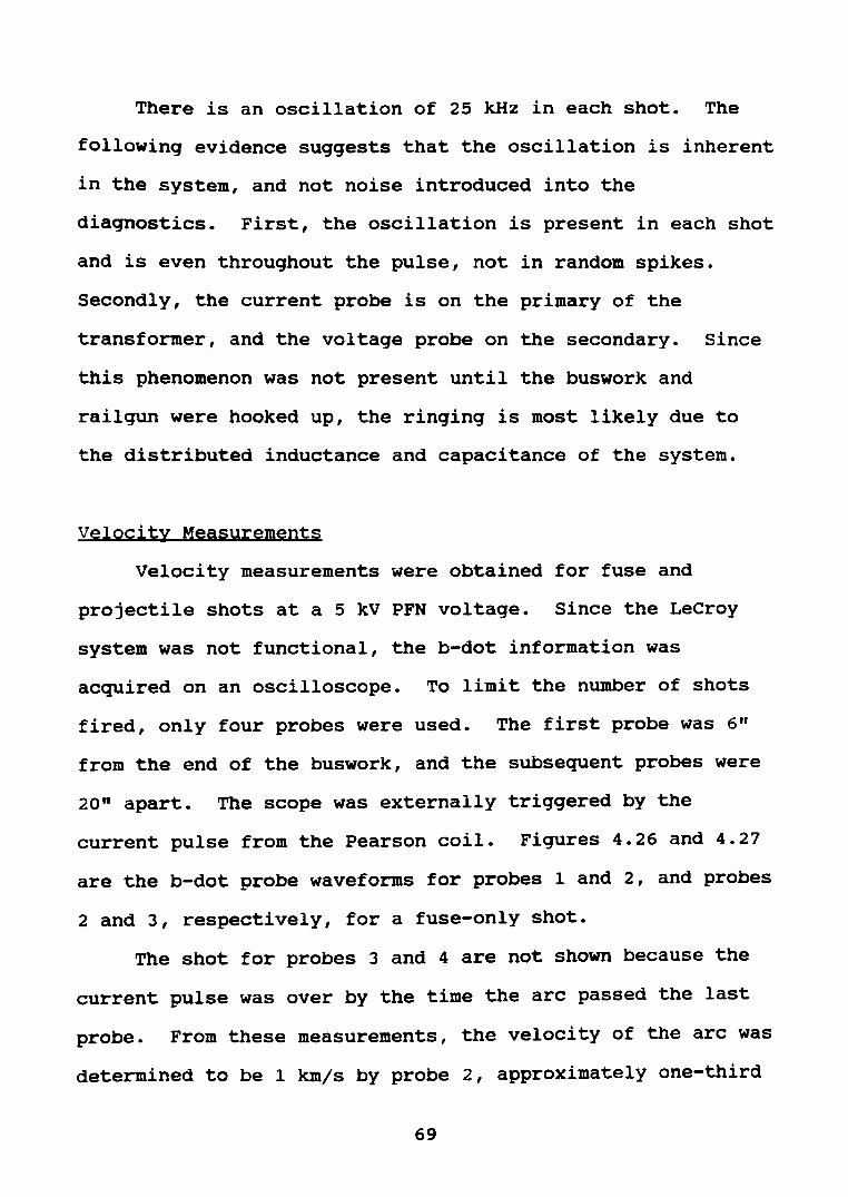
There is an oscillation of 25 kHz in each shot. The
following evidence suggests that the oscillation is inherent
in the system, and not noise introduced into the
diagnostics. First, the oscillation is present in each shot
and is even throughout the pulse, not in random spikes.
Secondly, the current probe is on the primary of the
transformer, and the voltage probe on the secondary. Since
this phenomenon was not present until the buswork and
railgun were hooked up, the ringing is most likely due to
the distributed inductance and capacitance of the system.
Velocity Measurements
Velocity measurements were obtained for fuse and
projectile shots at a 5 kV PFN voltage. Since the LeCroy
system was not functional, the b-dot information was
acquired on an oscilloscope. To limit the number of shots
fired, only four probes were used. The first probe was 6 11
from the end of the buswork, and the subsequent probes were
20" apart. The scope was externally triggered by the
current pulse from the Pearson coil. Figures 4.26 and 4.27
are the b-dot probe waveforms for probes 1 and 2, and probes
2 and 3, respectively, for a fuse-only shot.
The shot for probes 3 and 4 are not shown because the
current pulse was over by the time the arc passed the last
probe. From these measurements, the velocity of the arc was
determined to be 1 km/s by probe 2, approximately one-third
69
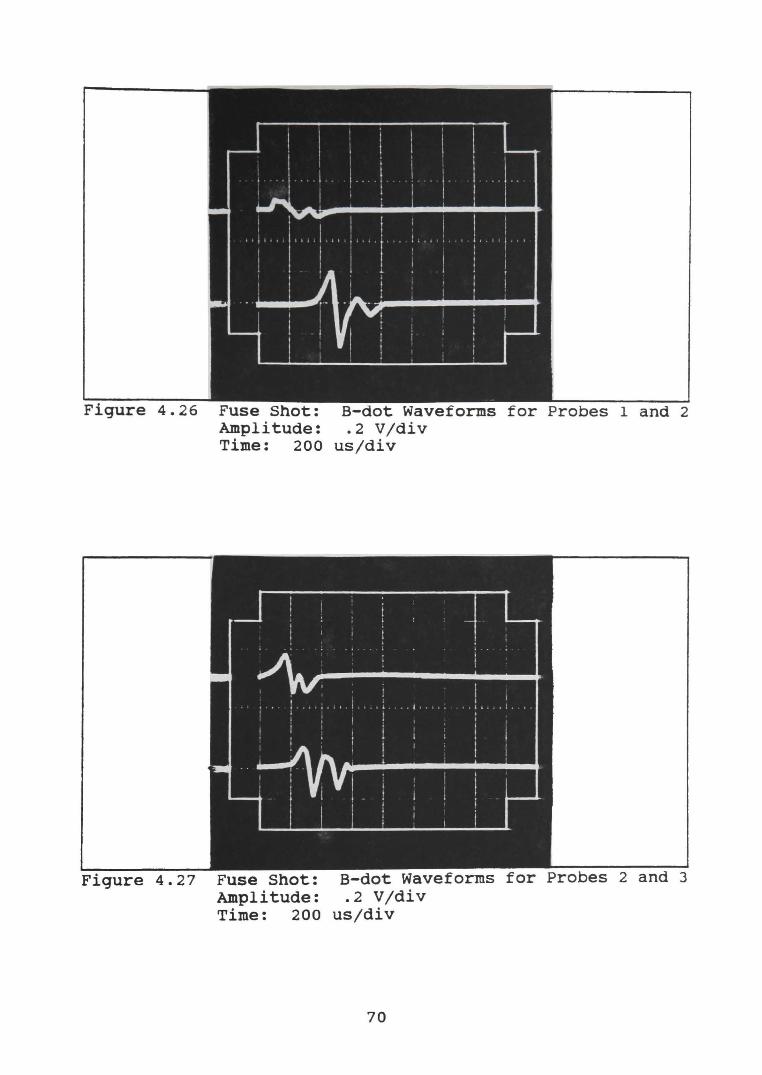
Figure 4.26 Fuse Shot: B-dot Waveforms for Probes 1 and 2 Amplitude: .2 V/div Time: 200 usjdiv
Figure 4.27 Fuse Shot: B-dot Waveforms Amplitude: .2 V/div Time: 200 usjdiv
70

the length of the bore, and 4.2 km/s by probe 3, two-thirds
the length. The presence of more than one rising and
falling impulse in the b-dot probe data suggests that a
secondary arc formed, closely following the first arc.
The data for the projectile is not shown, because it is
not particularly useful. The projectile reached a velocity
of .5 kmjs by probe 2. However, the current had decreased
sufficiently by probe 3 so as not to obtain any data.
71

CHAPTER V
CONCLUSIONS
The power supply has been tested into an ignitron load,
and into the railgun, with and without the pulse
transformer. The PFN behaved as predicted by PSPICE, with a
lower peak current. This was attributed to the parasitic
losses in the components and connections.
When the PFN was tested directly into the railgun
without the pulse transformer, the current waveshape was
retained, but the amplitude was drastically reduced. This
effect was unexpected because the railgun impedance is
comparable to the ignitron impedance. However, the losses
could be due, in part, to the losses in the railgun load.
For these tests, the railgun was fired at atmospheric
pressure, not in a vacuum, and the fuse was fairly
resistive. Also, shown in the high-current tests to the
railgun, using a wider fuse generated a higher current. The
fuse used for the low current shot was a spring that covered
only a small portion of the back of the projectile.
Although the maximum railgun current was not determined, it
was demonstrated that the railgun load did not distort the
pulse shape.
The PSPICE transformer model shows that the transformer
will retain the pulse shape for a 500 kA shot. For higher
currents, the effect of the transformer droop will become
72
significant. The actual data taken of pulsing the
transformer into a short circuit load shows that the
transformer retains the pulse shape very well. There is a
noticeable droop towards the end of the pulse, due partly to
the limitations of the Rogowski coil used to measure the
secondary current.
The current into the railgun for the high-current shots
is seriously limited by the contact resistance in the joints
of the buswork. The contact resistance can be decreased by
using a conducting grease specifically made for high current
contacts, but the cost is prohibitively high. The buswork
can be modified to minimize the discontinuities in the
system, without a complete redesign. Perhaps a modification
in the buswork will also eliminate the oscillations in the
output current and voltage signals.
If this step does not sufficiently increase the current
delivered to the railgun, two steps can be taken. The
transformer can be hooked up 10:1 with little difficulty,
but the secondary voltage would be lower. An easier, and
probably better, alternative is to increase the charging
voltage of the PFN. To generate 100 kA, the design voltage
for the system is 5 kV. The capacitors can be safely
charged to 11 kV to create a higher output current.
The velocity data will be more accurate once the data
acquisition system is operational. The existing
measurements suggest that the current pulse is finished
73

before the projectile reaches the muzzle of the gun. The
projectile velocity will level off once the magnetic energy
is gone. Ideally, the zero-crossing point of the current
pulse should coincide with the projectile exiting the bore.
The velocity measurements should be reevaluated once
the projectile is fired through the preinjector gun and
also with a higher railgun current. When a projectile is
fired from a standing start, energy is wasted on overcoming
the initial frictional forces. By using the preinjector
gun, the magnetic energy will not have to overcome the
initial friction, and the projectile will have an initial
velocity of approximately 300 mjs. Increasing the railgun
current will not increase the pulse length, but the
projectile will be moving faster, and will take less time to
travel down the bore.
This thesis has demonstrated the use of a pulse forming
network, pulse transformer power supply to drive a railgun
load at high currents. Although this type of power supply
is not new, it has never been used to power a railgun. This
system has the following advantages: the PFN can deliver a
shaped, tunable, high-current pulse, the transformer
provides better impedance matching and steps up the current
without compromising the pulse length, and the controls are
not complex.
74

REFERENCES
[1] Headley, Clifford. Interferometric Measurement of Plasma Armature Electron Density Profile in a Railgun Simulator. Master's Thesis, University of Texas at Arlington, 1988.
[2] Marshall, R.A. and Rashleigh, S.C. "Electromagnetic Acceleration of Macroparticles to High Velocities." Journal of Applied Physics, Vol. 49, [4], April 1978.
[3] Baker, M.C. and O'Hair, E.A. ''Investigation of Hybrid Armature Railgun Performance." submitted to SDIO, Kinetic Energy Branch, February 1990.
[4] Parker, J.V. "Why Plasma Armature Railguns Don't Work." IEEE Transactions on Magnetics, Vol. 25, [1], January 1989.
[5] Stanford, E.R. The Design of an Electrolytic Capacitor Based. Pulse Forming Network. Power Supply for a Railgun Simulator. Master's Thesis, University of Texas at Arlington, 1989.
[6] Pulsed Power Short Course. Texas Tech University, Pulsed Power Laboratory, Vol. 2, Lubbock, Texas 1989.
[7] Sarjeant, W.J. and Dollinger, R.E. High Power Electronics. 1st ed. Blue Ridge Summit, PA: TAB BOOKS Inc., 1989.
[8] Reed, Kim. "Using Pulse Forming Networks for Railgun Energy Sources." University of Texas at Arlington, 1985. unpublished.
[9] Glasoe, G.N. and Lebacqz, J.V. Pulse Generators. 1st ed. New York, NY: Dover Publications, 1965.
[10] Smith, Bret. Design and Construction of a Three Hundred kA Breech Simulation Railgun. Master's Thesis, Texas Tech University, 1989.
[11] Knoepfel, H. Pulsed High Magnetic Fields. 1st ed. London, England: North-Holland Publishing Co., 1970.
75

[12] Jiles, D.C. and Atherton, D.L. "Theory of Ferromagnetic Hysteresis." Journal of Magnetism and Magnetic Material, Vol. 61, [1], 1986.
76

APPENDIX
PSPICE LISTINGS FOR CHAPTER IV SIMULATIONS
77

PFN 1 IGNITRON LOAD I
1 PFN Cl 1 0 1.652M IC=5KV Dl 0 1 DCAP Ll 2 1 1.25U C2 2 0 1.652M IC=5KV D2 0 2 DCAP L2 3 2 1.25U C3 3 0 1.652M IC=5KV D3 0 3 DCAP L3 4 3 1.25U C4 4 0 1.652M IC=5KV D4 0 4 DCAP L4 5 4 1.25U C5 5 0 1.652M IC=5KV D5 0 5 DCAP I
1 IGNITRON SWITCH LOAD SLOAD 5 0 20 0 IGNITRON VSW 20 0 PWL(O 0 .05U .5 .lU 1 lOU 1) RSW 20 0 lOOMEG I
.MODEL DCAP D
.MODEL IGNITRON VSWITCH (RON=.003)
.TRAN 20U 2M UIC
.PROBE
.END
78

PULSE TRANSFORMER 'MATCHED LOAD I
'IDEAL INPUT CURRENT PULSE !PULSE 1 0 PULSE(O lOOKA 0 SOU SOU 500U) I
'PULSE TRANSFORMER 5:1 LPRIM 1 0 60 LSEC 2 0 12 KTRAN LPRIM LSEC .9999 TPULSE I
'MATCHED RESISTIVE LOAD ROUT 2 0 .001 I
.MODEL TPULSE CORE (AREA=1206.45 PATH=279.4 GAP=.05 MS=600)
.TRAN 50U 1M
.OPTIONS (ITL5=0 RELTOL=.Ol)
.PROBE
.END
79

PULSE TRANSFORMER 'MATCHED LOAD I
'IDEAL INPUT CURRENT PULSE !PULSE 1 0 PULSE(O lOOKA 0 SOU SOU 500U) I
'PULSE TRANSFORMER 10:1 LPRIM 1 0 60 LSEC 2 0 6 KTRAN LPRIM LSEC .9999 TPULSE I
'MATCHED RESISTIVE LOAD ROUT 2 0 .001 I
.MODEL TPULSE CORE (AREA=1206.45 PATH=279.4 GAP=.05 MS=600)
.TRAN SOU 1M
.OPTIONS (ITL5=0 RELTOL=.Ol)
.PROBE
.END
so
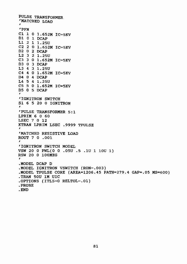
PULSE TRANSFORMER 'MATCHED LOAD ' 'PFN Cl 1 0 1.652M IC=5KV Dl 0 1 DCAP Ll 2 1 1.25U C2 2 0 1.652M IC=5KV D2 0 2 DCAP L2 3 2 1.25U C3 3 0 1.652M IC=5KV D3 0 3 DCAP L3 4 3 1.25U C4 4 0 1.652M IC=5KV D4 0 4 DCAP L4 5 4 1.25U C5 5 0 1.652M IC=5KV D5 0 5 DCAP ' 'IGNITRON SWITCH Sl 6 5 20 0 IGNITRON ' 'PULSE TRANSFORMER 5:1 LPRIM 6 0 60 LSEC 7 0 12 KTRAN LPRIM LSEC .9999 TPULSE ' 'MATCHED RESISTIVE LOAD ROUT 7 0 .001 ' 'IGNITRON SWITCH MODEL VSW 20 0 PWL(O 0 .05U .5 .lU 1 lOU 1) RSW 20 0 lOOMEG ' .MODEL DCAP D .MODEL IGNITRON VSWITCH (RON=.003) .MODEL TPULSE CORE (AREA=l206.45 PATH=279.4 GAP=.05 MS=600) .TRAN 50U 1M UIC .OPTIONS (ITL5=0 RELTOL=.Ol) .PROBE .END
81
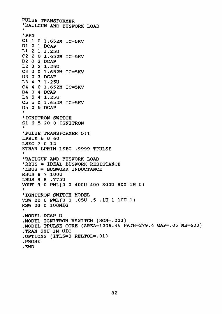
PULSE TRANSFORMER 'RAILGUN AND BUSWORK LOAD I
'PFN Cl 1 0 1.652M IC=5KV Dl 0 1 DCAP Ll 2 1 1.25U C2 2 0 1.652M IC=5KV D2 0 2 DCAP L2 3 2 1.25U C3 3 0 1.652M IC=5KV D3 0 3 DCAP L3 4 3 1.25U C4 4 0 1.652M IC=5KV D4 0 4 DCAP L4 5 4 1.25U C5 5 0 1.652M IC=5KV D5 0 5 DCAP I
'IGNITRON SWITCH Sl 6 5 20 0 IGNITRON I
'PULSE TRANSFORMER 5:1 LPRIM 6 0 60 LSEC 7 0 12 KTRAN LPRIM LSEC .9999 TPULSE I
'RAILGUN AND BUSWORK LOAD 'RBUS = IDEAL BUSWORK RESISTANCE 'LBUS = BUSWORK INDUCTANCE RBUS 8 7 lOOU LBUS 9 8 .775U VOUT 9 0 PWL(O 0 400U 400 800U 800 1M 0) I
'IGNITRON SWITCH MODEL VSW 20 0 PWL(O 0 .05U .5 .lU 1 lOU 1) RSW 20 0 lOOMEG I
.MODEL DCAP D
.MODEL IGNITRON VSWITCH (RON=.003)
.MODEL TPULSE CORE (AREA=1206.45 PATH=Z79.4 GAP=.05 MS=600)
.TRAN 50U 1M UIC
.OPTIONS (ITL5=0 RELTOL=.Ol)
.PROBE
.END
82

PULSE TRANSFORMER 'CONTACT RESISTANCE , 'PFN Cl 1 0 1.652M IC=SKV Dl 0 1 DCAP Ll 2 1 1.25U C2 2 0 1.652M IC=SKV D2 0 2 DCAP L2 3 2 1.25U C3 3 0 1.652M IC=SKV D3 0 3 DCAP L3 4 3 1.25U C4 4 0 1.652M IC=SKV D4 0 4 DCAP L4 5 4 1.25U C5 5 0 1.652M IC=SKV D5 0 5 DCAP , 'IGNITRON SWITCH Sl 6 5 20 0 IGNITRON , 'PULSE TRANSFORMER 5:1 LPRIM 6 0 60 LSEC 7 0 12 KTRAN LPRIM LSEC .999 TPULSE , 'RAILGUN AND BUSWORK LOAD 'RBUS = IDEAL BUSWORK RESISTANCE + CONTACT RESISTANCE 'LBUS = BUSWORK INDUCTANCE RBUS 8 7 .002 LBUS 9 8 .775U VOUT 9 0 PWL(O 0 400U 400 800U 800 1M 0) , 'IGNITRON SWITCH MODEL VSW 20 0 PWL(O 0 .05U .5 .lU 1 lOU 1) RSW 20 0 lOOMEG , .MODEL DCAP D .MODEL IGNITRON VSWITCH (RON=.003) .MODEL TPULSE CORE (AREA=1206.45 PATH=279.4 GAP=.05 MS=600) .TRAN SOU 1M UIC .OPTIONS (ITL5=0 RELTOL=.Ol) .PROBE .END
83
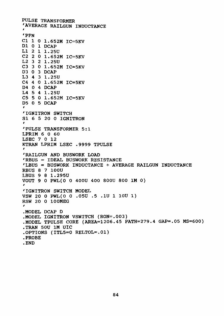
PULSE TRANSFORMER 'AVERAGE RAILGUN INDUCTANCE I
'PFN Cl 1 0 1.652M IC=5KV Dl 0 1 DCAP Ll 2 1 1.25U C2 2 0 1.652M IC=5KV L2 3 2 1.25U C3 3 0 1.652M IC=5KV D3 0 3 DCAP L3 4 3 1.25U C4 4 0 1.652M IC=5KV D4 0 4 DCAP L4 5 4 1.25U C5 5 0 1.652M IC=5KV D5 0 5 DCAP I
'IGNITRON SWITCH Sl 6 5 20 0 IGNITRON I
'PULSE TRANSFORMER 5:1 LPRIM 6 0 60 LSEC 7 0 12 KTRAN LPRIM LSEC .9999 TPULSE I
'RAILGUN AND BUSWORK LOAD 'RBUS = IDEAL BUSWORK RESISTANCE 'LBUS = BUSWORK INDUCTANCE + AVERAGE RAILGUN INDUCTANCE RBUS 8 7 lOOU LBUS 9 8 1.295U VOUT 9 0 PWL(O 0 400U 400 800U 800 1M 0) I
'IGNITRON SWITCH MODEL VSW 20 0 PWL(O 0 .05U .5 .lU 1 lOU 1) RSW 20 0 lOOMEG I
.MODEL DCAP D
.MODEL IGNITRON VSWITCH (RON=.003)
.MODEL TPULSE CORE (AREA=l206.45 PATH=279.4 GAP=.05 MS=600)
.TRAN 50U 1M UIC
.OPTIONS (ITL5=0 RELTOL=.Ol)
.PROBE
.END
84
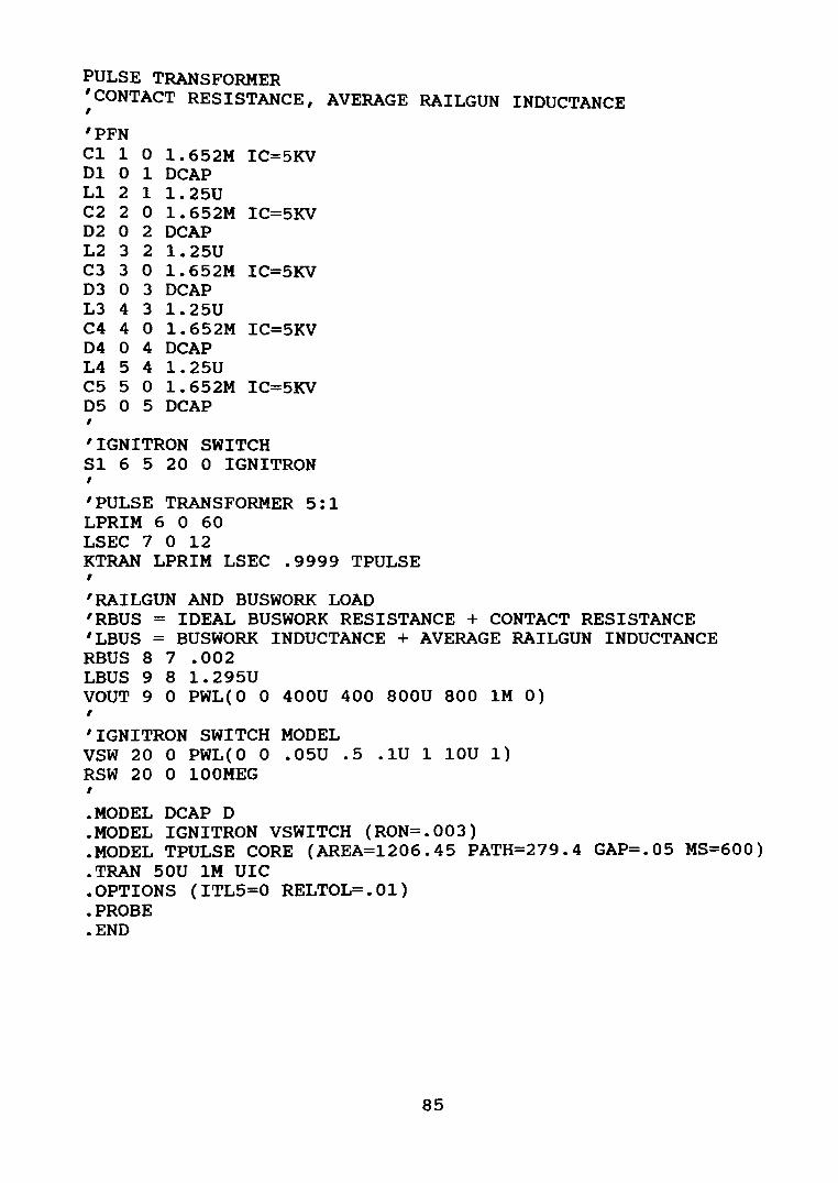
PULSE TRANSFORMER 'CONTACT RESISTANCE, AVERAGE I
'PFN Cl 1 0 1.652M IC=5KV Dl 0 1 DCAP Ll 2 1 1.25U C2 2 0 1.652M IC=5KV D2 0 2 DCAP L2 3 2 1.25U C3 3 0 1.652M IC=SKV D3 0 3 DCAP L3 4 3 1.25U C4 4 0 1.652M IC=5KV 04 0 4 DCAP L4 5 4 1.25U cs 5 0 1.652M IC=5KV DS 0 5 DCAP I
'IGNITRON SWITCH Sl 6 5 20 0 IGNITRON , 'PULSE TRANSFORMER 5:1 LPRIM 6 0 60 LSEC 7 0 12
RAILGUN INDUCTANCE
KTRAN LPRIM LSEC .9999 TPULSE I
'RAILGUN AND BUSWORK LOAD 'RBUS = IDEAL BUSWORK RESISTANCE + CONTACT RESISTANCE 'LBUS = BUSWORK INDUCTANCE + AVERAGE RAILGUN INDUCTANCE RBUS 8 7 .002 LBUS 9 8 1.295U VOUT 9 0 PWL(O 0 400U 400 800U 800 1M 0) I
'IGNITRON SWITCH MODEL VSW 20 0 PWL(O 0 .OSU .5 .lU 1 lOU 1) RSW 20 0 lOOMEG I
.MODEL DCAP D
.MODEL IGNITRON VSWITCH (RON=.003)
.MODEL TPULSE CORE (AREA=1206.45 PATH=279.4 GAP=.OS MS=600)
.TRAN SOU 1M UIC
.OPTIONS (ITLS=O RELTOL=.Ol)
.PROBE
.END
85