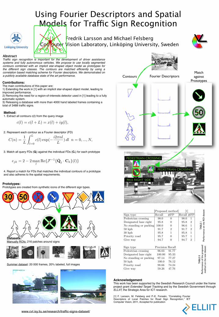
AbstractTraffic sign recognition is important for the development of driver assistance systems and fully autonomous vehicles. We propose to use locally segmented contours combined with an implicit star-shaped object model as prototypes for the different sign classes. The contours are matched efficiently by using a correlation based matching scheme for Fourier descriptors. We demonstrated on a publicly available database state of the art performance.

Contributions:The main contributions of this paper are:1) Extending the work in [1] with an implicit star-shaped object model, leading to improved performance.2) Removing the need for a region-of-interests detector used in [1] leading to a fully automatic system.3) Releasing a database with more than 4000 hand labeled frames containing a total of 3488 traffic signs.

Fredrik Larsson and Michael FelsbergComputer Vision Laboratory, Linköping University, Sweden

Using Fourier Descriptors and Spatial Models for Traffic Sign Recognition

AcknowledgementThis work has been supported by the Swedish Research Council under the frame project grant Extended Target Tracking and by the Swedish Government through ELLIIT, the Strategic Area for ICT research.

1277107930Image000011.jpg

SIDE_ROAD, PEDESTRIAN_CROSSING

SIDE_ROAD, PEDESTRIAN_CROSSINGVISIBLE, PEDESTRIAN_CROSSING

VISIBLE, PASS_RIGHT_SIDEVISIBLE, PRIORITY_ROAD

1277389846Image000071.jpgMisc. signs

VISIBLE, 120_SIGN

www.cvl.isy.liu.se/research/traffic-signs-dataset/

Datasets:Manually ROIs: 216 patches around signs

Summer dataset: 20 000 frames, 20% labeled, full images

Fig. 3. Extracted local features (green contours) and correspondingvectors (red arrows) pointing towards the center of the traffic sign.

vk is simply the vector from the center of the local featureto the center of the object, see Fig. 3. This can be seenas a simple implicit star-shaped object model [14] whereeach local feature is connected to the center of the object.The combination of FDs and corresponding spatial vectorsgives the final traffic sign prototype as

P = {(Ck,vk)} k = 1..K (11)

where K is the total number of contours for the prototype.

D. Matching Sign Prototypes

From a query image J contours qj are extracted, seeFig. 1 left, and represented by their FDs Qj . For eachsign prototype, all prototype contours Ck are comparedto all extracted contours Qj using (8):

ejk = 2− 2maxl

Re{F−1{Qj ·Ck}(l)} . (12)

This results in the binary matrix M = (m)jk of matchedcontours, see Fig. 1 left, with

mjk =

�1 ejk ≤ θk0 ejk > θk

(13)

where θk is a manually selected threshold for each pro-totype contour k.

The next step is to verify which combinations ofmatched contours Qj fit to the spatial configuration ofthe sign prototype. This is done by a cascaded matchingscheme. For each individual match mjk, we obtain bymeans of (10) parameters sk and tk and compute anestimate v�

jk = sjkvk + tjk.The vector v�

j1 defines a hypothesized prototype center.We then go through all prototype contours k = 2 . . .Kand verify for all mik �= 0, i �= j, that sik/sj1 issufficiently close to 1 and that v�

ik is sufficiently closeto the hypothesized prototype center. These contours areconsistent with respect to scale and location and if onlyif sufficiently many contours are consistent, a detectionof the corresponding sign is flagged, see Fig. 1 right.

E. Dataset

A dataset has been created by recording sequences fromover 350 km of Swedish highways and city roads. A 1.3mega-pixel color camera, a Point-Grey Chameleon, wasplaced inside a car on the dashboard looking out of thefront window. The camera was pointing slightly to theright, in order to cover as many relevant signs as possible.

(a) (b) (c) (d) (e) (f) (g)

(A) (B) (C) (D) (E) (F) (G)Fig. 4. First row: Synthetic signs used to create models. Second row:Corresponding real world examples.

The lens had a focal length of 6.5mm, resulting in approx-imately 41 degrees field of view. Typical speed signs onmotorways are about 90 cm wide, which corresponds toa size of about 50 pixel if they are to be detected at adistance of about 30 m.

A human operator started the recording whenever atraffic sign was visible and stopped the recording whenno more signs were visible. In total, in over 20 000frames have been recorded of which every fifth frame hasbeen manually labeled. The label for each sign containssign type (pedestrian crossing, designated lane right, nostanding or parking, priority road, give way, 50 kph, or 30kph), visibility status (occluded, blurred, or visible) androad status (whether the signs is on the road being traveledor on a side road). The entire database including groundtruth is available on https://www.cvl.isy.liu.se/research/traffic-signs-dataset.

III. EXPERIMENTS

Synthetic images of Swedish road signs, see bottomrow of Fig. 4, were used for creating models accordingto the methodology described in Sec. II-C. The signmodels were then matched against real images from twodatasets. The first dataset, denoted Manually ROIs dataset,is the one used in [5] which is using patches frombounding boxes of 200x200 pixels, see Fig. 4. The secondevaluation was done on the the newly collected dataset,denoted Summer dataset, see Sec. II-E. All processing isdone frame wise not using temporal clues.

Note that the evaluation was done using grey scaleimages and do not use the distinct colors of the signs as adescriptor. The images used correspond to the red channelof a normal color camera. This is easily achieved byplacing a red-pass filter in front of an ordinary monochro-matic camera. Using normal grey-scale conversion wouldbe problematic since some of the signs are isoluminant,e.g. sign (c) in Fig. 4. The reason for not using colors isthat color cameras have lower frame rates given a fixedbandwidth and resolution. High frame rates are crucialfor cameras to be used within the automotive industry.Higher frame rates mean for example higher accuracywhen estimating the velocity of approaching cars.

A. Results Manually ROIs dataset

The first dataset is used in order to compare tothe reported results in [5] and contains 316 regions-of-interests (ROIs) of 200x200 pixels, see Fig. 4. The ROIswere manually extracted around 216 signs and 100 non-signs. The result is summarized in table I. This dataset

Fig. 3. Extracted local features (green contours) and correspondingvectors (red arrows) pointing towards the center of the traffic sign.

vk is simply the vector from the center of the local featureto the center of the object, see Fig. 3. This can be seenas a simple implicit star-shaped object model [14] whereeach local feature is connected to the center of the object.The combination of FDs and corresponding spatial vectorsgives the final traffic sign prototype as

P = {(Ck,vk)} k = 1..K (11)

where K is the total number of contours for the prototype.

D. Matching Sign Prototypes

From a query image J contours qj are extracted, seeFig. 1 left, and represented by their FDs Qj . For eachsign prototype, all prototype contours Ck are comparedto all extracted contours Qj using (8):

ejk = 2− 2maxl

Re{F−1{Qj ·Ck}(l)} . (12)

This results in the binary matrix M = (m)jk of matchedcontours, see Fig. 1 left, with

mjk =

�1 ejk ≤ θk0 ejk > θk

(13)

where θk is a manually selected threshold for each pro-totype contour k.

The next step is to verify which combinations ofmatched contours Qj fit to the spatial configuration ofthe sign prototype. This is done by a cascaded matchingscheme. For each individual match mjk, we obtain bymeans of (10) parameters sk and tk and compute anestimate v�

jk = sjkvk + tjk.The vector v�

j1 defines a hypothesized prototype center.We then go through all prototype contours k = 2 . . .Kand verify for all mik �= 0, i �= j, that sik/sj1 issufficiently close to 1 and that v�

ik is sufficiently closeto the hypothesized prototype center. These contours areconsistent with respect to scale and location and if onlyif sufficiently many contours are consistent, a detectionof the corresponding sign is flagged, see Fig. 1 right.

E. Dataset

A dataset has been created by recording sequences fromover 350 km of Swedish highways and city roads. A 1.3mega-pixel color camera, a Point-Grey Chameleon, wasplaced inside a car on the dashboard looking out of thefront window. The camera was pointing slightly to theright, in order to cover as many relevant signs as possible.

(a) (b) (c) (d) (e) (f) (g)

(A) (B) (C) (D) (E) (F) (G)Fig. 4. First row: Synthetic signs used to create models. Second row:Corresponding real world examples.

The lens had a focal length of 6.5mm, resulting in approx-imately 41 degrees field of view. Typical speed signs onmotorways are about 90 cm wide, which corresponds toa size of about 50 pixel if they are to be detected at adistance of about 30 m.

A human operator started the recording whenever atraffic sign was visible and stopped the recording whenno more signs were visible. In total, in over 20 000frames have been recorded of which every fifth frame hasbeen manually labeled. The label for each sign containssign type (pedestrian crossing, designated lane right, nostanding or parking, priority road, give way, 50 kph, or 30kph), visibility status (occluded, blurred, or visible) androad status (whether the signs is on the road being traveledor on a side road). The entire database including groundtruth is available on https://www.cvl.isy.liu.se/research/traffic-signs-dataset.

III. EXPERIMENTS

Synthetic images of Swedish road signs, see bottomrow of Fig. 4, were used for creating models accordingto the methodology described in Sec. II-C. The signmodels were then matched against real images from twodatasets. The first dataset, denoted Manually ROIs dataset,is the one used in [5] which is using patches frombounding boxes of 200x200 pixels, see Fig. 4. The secondevaluation was done on the the newly collected dataset,denoted Summer dataset, see Sec. II-E. All processing isdone frame wise not using temporal clues.

Note that the evaluation was done using grey scaleimages and do not use the distinct colors of the signs as adescriptor. The images used correspond to the red channelof a normal color camera. This is easily achieved byplacing a red-pass filter in front of an ordinary monochro-matic camera. Using normal grey-scale conversion wouldbe problematic since some of the signs are isoluminant,e.g. sign (c) in Fig. 4. The reason for not using colors isthat color cameras have lower frame rates given a fixedbandwidth and resolution. High frame rates are crucialfor cameras to be used within the automotive industry.Higher frame rates mean for example higher accuracywhen estimating the velocity of approaching cars.

A. Results Manually ROIs dataset

The first dataset is used in order to compare tothe reported results in [5] and contains 316 regions-of-interests (ROIs) of 200x200 pixels, see Fig. 4. The ROIswere manually extracted around 216 signs and 100 non-signs. The result is summarized in table I. This dataset

Prototypes:Prototypes are created from synthetic icons of the different sign types.

Traffic Sign Recognition Using FourierDescriptors and Spatial Models

Fredrik Larsson and Michael FelsbergComputer Vision Laboratory,

Linkoping University, SE-581 83 Linkoping, SwedenEmail: {larsson,mfe}@isy.liu.se

Abstract—Traffic sign recognition is important for the de-velopment of driver assistance systems and fully autonomousvehicles. Even though GPS navigator systems works wellfor most of the time, there will always be situations whenthey fail. In these cases, robust vision based systems arerequired. Traffic signs are designed to have distinct coloredfields separated by sharp boundaries. We propose to uselocally segmented contours combined with an implicit star-shaped object model as prototypes for the different signclasses. The contours are described by Fourier descriptors.Matching of a query image to the sign prototype database isdone by exhaustive search. This is done efficiently by usingthe correlation based matching scheme for Fourier descrip-tors and a fast cascaded matching scheme for enforcingthe spatial requirements. We demonstrated on a publiclyavailable database state of the art performance.

I. INTRODUCTION

Traffic sign recognition is important for the develop-ment of driver assistance systems and fully autonomousvehicles. Even though GPS navigator systems work wellfor most of the time, there will always be situationswhen no GPS-signal is available or when the map isinvalid, temporary sign installations near road works justto mention one example. In these cases, robust visionbased systems are required, preferably making use ofmonochromatic images.

A. Related WorkMany different approaches to traffic sign recognition

have been proposed and there are commercial visionbased systems available, for example in VolkswagenPhaeton, Saab 9-5 and in the BMW 5 and 7 series.

One common approach is to threshold in a carefullychosen color space, e.g. HSV [1], HSI [2] or CBH [3],in order to obtain a (set of) binary image(s). This isthen followed by detection and classification using theauthors favorite choice of classifier, e.g. support vectormachines [4] or Neural networks [1], [2]. Another com-mon approach is to consider an edge map using e.g.Fourier descriptors [5], Hough transform [6] or distancetransforms [7]. For an excellent overview of existingapproaches see [2].

One thing that most published methods have in com-mon is that they report excellent results on their own datasets. Typically they achieve more than 95% recognitionrate with very few false positives. However, there areunfortunately no publicly available database for compar-ing different road sign recognition systems. Meaning that

PEDESTRIAN_CROSSING

PASS_RIGHT_SIDE

PEDESTRIAN_CROSSINGPEDESTRIAN_CROSSING

Fig. 1. Left: Contours that matched any of the contours in the pedestriancrossing prototype are shown in a non-yellow color. Right: The finalresults after matching against all sign prototypes.

most authors report results on their own dataset and donot provide any means of comparing against their method.One of the main contributions of this paper is to provide alabeled database of more than 4000 frames captured whiledriving 350 km on highways and in city environment.

B. Main ContributionThe main contributions of this paper are:1) Extending the work [5] with an implicit star-shaped

object model, leading to improved performance.2) Removing the need for a region-of-interests detector

used in [5], leading to a fully automatic system.3) Releasing a database with more than 4000 hand

labeled frames (more than 3488 traffic signs).

II. METHODS

The proposed method consists of three steps: extrac-tion of Fourier descriptors (FDs), matching of FDs, andmatching of previously acquired prototypes with spatialmodels.

A. Fourier DescriptorsFourier descriptors (FDs) [8] is a classic and still

popular method for contour matching. The key idea is toapply the Fourier transform to a periodic representationof the boundary, which results in a shape descriptor in thefrequency domain.

In line with Granlund [8], the closed contour c withcoordinates x and y is parameterized as a complex valuedperiodic function

c(l) = c(l + L) = x(l) + iy(l), (1)

where L is the contour length, usually given by thenumber of contour samples.1 By taking the 1D Fourier

1We treat contours as continuous functions here, where the contoursamples can be thought as of impulses with appropriate weights.

transform of c, the Fourier coefficients C are obtained as

C(n) =1

L

� L

l=0c(l) exp(− i2πnl

L) dl n = 0, ..., N, (2)

where N ≤ L is the descriptor length.One reason for the popularity of FDs is that they are

easy to interpret. Each coefficient has a clear physicalmeaning and using only a few of the low frequencycoefficients is equivalent to smoothing the contour. SeeFig. 2 where we reconstruct a pedestrian outline startingwith two low frequency coefficients and gradually addmore and more high frequency components.

2 3 4 5 6 8 10

12 14 16 32 64 128 256

Fig. 2. Reconstruction of a detail from a Swedish pedestrian crossingsign using increasing number (shown above respective contour) ofFourier coefficients.

Another strength and reason for popularity of FDsis their behavior under geometric transformations. TheDC component C(0) is the only one that is affectedby translations c0 of the curve c(l) �→ c(l) + c0. Bydisregarding this coefficient, the remaining N − 1 co-efficients are invariant under translation. Scaling of thecontour, i.e. c(l) �→ ac(l), affects the magnitude of thecoefficients and the coefficients can thus be made scaleinvariant by normalizing with the energy (after C(0) hasbeen removed). Without loss of generality, we assumethat �C�2 = 1 (� · �2 denotes the quadratic norm) andC(0) = 0 in what follows.

Rotating the contour c with φ radians counter clock-wise corresponds to multiplication of (1) with exp(iφ),which adds a constant offset to the phase of the Fouriercoefficients

c(l) �→ exp(iφ)c(l) ⇒ C(n) �→ exp(iφ)C(n) . (3)

Furthermore, if the index l of the contour is shifted by∆l, a linear offset is added to the Fourier phase, i.e. thespectrum is modulated

c(l) �→ c(l −∆l) ⇒ C(n) �→ C(n) exp(− i2πn∆l

L) .

(4)When we use the term shift we always refer to a shiftin the starting point for sampling, this should not beconfused with translation which we use to denote spatialtranslation of the entire contour.

B. Matching of FDsSince rotation and index-shift result in modulations of

the FD, it has been suggested to neglect phase infor-mation in order to be invariant to these transformations.

However, as pointed out by Oppenheim and Lim [9],most information is contained in the phase and simplyneglecting it means to throw away information. Matchingof magnitudes ignores a major part of the signal structuresuch that the matching is less specific. According to (3)and (4), the phase of each FD component is modifiedby a rotation of the corresponding trigonometric basisfunction, either by a constant offset or by a linear offset.Considering magnitudes only can be seen as finding theoptimal rotation of all different components of the FDindependently. That is, given a FD of length N −1, mag-nitude matching corresponds to finding N − 1 differentrotations instead of estimating two degrees of freedom(constant and slope). Due to the removal of N−3 degreesof freedom, two contours can be very different eventhough the magnitude in each FD component is the same.

Recently, a new efficient correlation based matchingmethod for FDs was proposed by Larsson et al. [5]. Thisapproach is partly similar to established methods suchas [10], [11], but differs in some respects: Complex FDsare directly correlated to find the relative rotation betweentwo FDs without numerically solving equation systems:Let T denote a transformation corresponding to rotationand index-shift. Let c1 and c2 denote two normalizedcontours, then

minT

�c1 − T c2�2 = 2− 2maxl

|r12(l)| (5)

where |·| denotes the complex modulus and the cross cor-relation r12 is computed between the Fourier descriptorsC1 and C2 according to [12], p. 244–245,

r12(k) = (c1 � c2)(k).=

� L

0c1(l)c2(k + l) dl (6)

= F−1{C1 · C2}(k) . (7)

In particular, if c�1 and c�2 denote two contours so thatc�2 = T �c�1, where T � denotes a transformation coveringscaling, translation, rotation and index-shift, then

minT

�c�1 − T c�2�2 = 2− 2maxl

|r12(l)| = 0 . (8)

The parameters of the transformation T that minimizes(8) are given as

∆l = argmaxl

|r12(l)| φ = arg r12(∆l) (9)

s =(�∞

n=1 |C �1(n)|2)

12

(�∞

n=1 |C �2(n)|2)

12

t = C �1(0)− C �

2(0)(10)

C. Sign PrototypesA traffic sign prototype is created from a synthetic

image of the traffic sign, see first row in Fig. 4. Thesynthetic image is low-pass filtered before local contoursare extracted using Maximally Stable Extremal Regions(MSER)[13]. Each extracted contour ck is described byits Fourier descriptor Ck.

In order to describe the spatial relationships betweenthe local features an extra component vk is added, cre-ating a pair (Ck,vk) where the first component capturesthe local geometry (contour) and the second componentthe global geometry of the sign. This second component

Fig. 3. Extracted local features (green contours) and correspondingvectors (red arrows) pointing towards the center of the traffic sign.

vk is simply the vector from the center of the local featureto the center of the object, see Fig. 3. This can be seenas a simple implicit star-shaped object model [14] whereeach local feature is connected to the center of the object.The combination of FDs and corresponding spatial vectorsgives the final traffic sign prototype as

P = {(Ck,vk)} k = 1..K (11)

where K is the total number of contours for the prototype.

D. Matching Sign Prototypes

From a query image J contours qj are extracted, seeFig. 1 left, and represented by their FDs Qj . For eachsign prototype, all prototype contours Ck are comparedto all extracted contours Qj using (8):

ejk = 2− 2maxl

Re{F−1{Qj ·Ck}(l)} . (12)

This results in the binary matrix M = (m)jk of matchedcontours, see Fig. 1 left, with

mjk =

�1 ejk ≤ θk0 ejk > θk

(13)

where θk is a manually selected threshold for each pro-totype contour k.

The next step is to verify which combinations ofmatched contours Qj fit to the spatial configuration ofthe sign prototype. This is done by a cascaded matchingscheme. For each individual match mjk, we obtain bymeans of (10) parameters sk and tk and compute anestimate v�

jk = sjkvk + tjk.The vector v�

j1 defines a hypothesized prototype center.We then go through all prototype contours k = 2 . . .Kand verify for all mik �= 0, i �= j, that sik/sj1 issufficiently close to 1 and that v�

ik is sufficiently closeto the hypothesized prototype center. These contours areconsistent with respect to scale and location and if onlyif sufficiently many contours are consistent, a detectionof the corresponding sign is flagged, see Fig. 1 right.

E. Dataset

A dataset has been created by recording sequences fromover 350 km of Swedish highways and city roads. A 1.3mega-pixel color camera, a Point-Grey Chameleon, wasplaced inside a car on the dashboard looking out of thefront window. The camera was pointing slightly to theright, in order to cover as many relevant signs as possible.

(a) (b) (c) (d) (e) (f) (g)

(A) (B) (C) (D) (E) (F) (G)Fig. 4. First row: Synthetic signs used to create models. Second row:Corresponding real world examples.

The lens had a focal length of 6.5mm, resulting in approx-imately 41 degrees field of view. Typical speed signs onmotorways are about 90 cm wide, which corresponds toa size of about 50 pixel if they are to be detected at adistance of about 30 m.

A human operator started the recording whenever atraffic sign was visible and stopped the recording whenno more signs were visible. In total, in over 20 000frames have been recorded of which every fifth frame hasbeen manually labeled. The label for each sign containssign type (pedestrian crossing, designated lane right, nostanding or parking, priority road, give way, 50 kph, or 30kph), visibility status (occluded, blurred, or visible) androad status (whether the signs is on the road being traveledor on a side road). The entire database including groundtruth is available on https://www.cvl.isy.liu.se/research/traffic-signs-dataset.

III. EXPERIMENTS

Synthetic images of Swedish road signs, see bottomrow of Fig. 4, were used for creating models accordingto the methodology described in Sec. II-C. The signmodels were then matched against real images from twodatasets. The first dataset, denoted Manually ROIs dataset,is the one used in [5] which is using patches frombounding boxes of 200x200 pixels, see Fig. 4. The secondevaluation was done on the the newly collected dataset,denoted Summer dataset, see Sec. II-E. All processing isdone frame wise not using temporal clues.

Note that the evaluation was done using grey scaleimages and do not use the distinct colors of the signs as adescriptor. The images used correspond to the red channelof a normal color camera. This is easily achieved byplacing a red-pass filter in front of an ordinary monochro-matic camera. Using normal grey-scale conversion wouldbe problematic since some of the signs are isoluminant,e.g. sign (c) in Fig. 4. The reason for not using colors isthat color cameras have lower frame rates given a fixedbandwidth and resolution. High frame rates are crucialfor cameras to be used within the automotive industry.Higher frame rates mean for example higher accuracywhen estimating the velocity of approaching cars.

A. Results Manually ROIs dataset

The first dataset is used in order to compare tothe reported results in [5] and contains 316 regions-of-interests (ROIs) of 200x200 pixels, see Fig. 4. The ROIswere manually extracted around 216 signs and 100 non-signs. The result is summarized in table I. This dataset

Method:1. Extract all contours c(l) from the query image

2. Represent each contour as a Fourier descriptor (FD)

3. Match all query FDs (Qj) against the individual FDs (Ck) for each prototype

4. Report a match for FDs that matches the individual contours of a prototype and also adheres to the spatial requirements.

Contours Fourier DescriptorsMatch against

Prototypes

PEDESTRIAN_CROSSING

PASS_RIGHT_SIDE

PEDESTRIAN_CROSSINGPEDESTRIAN_CROSSING

PEDESTRIAN CROSSING

PEDESTRIAN CROSSING

PASS RIGHT SIDE

ROIs were manually extracted around 216 signs and 100 non-signs. The result

is summarized in table 1. This dataset is fairly simple and the proposed method

increases the already good performance of [10]. Using constraints on the spatial

arrangement of contours removes some of the false positives (FPs) while keeping

the same recall level or increasing it by allowing for less strict thresholds on the

individual contours. The classes Priority road and Give way are unaffected since

they consist of a single contour each, thus not benefiting from the added spatial

constraints.

Proposed method [1]

Sign type Recall #FP Recall #FP

Pedestrian crossing 98.0 0 98.0 1

Designated lane right 95.8 0 95.8 2

No standing or parking 100.0 0 96.6 1

50 kph 91.7 2 91.7 2

30 kph 95.8 1 95.8 1

Priority road 95.7 0 95.7 1

Give way 94.7 0 94.7 2

Table 1. Performance on the Manually ROIs dataset for the method presented in [10]

and the proposed algorithm.

3.2 Results Summer dataset

The second evaluation is done on the new Summer dataset, see Sec. 2.5 for details

regarding the dataset. The evaluation was limited to include signs for the road

being traveled on with a bounding box of at least 50x50 pixels, corresponding to

a sign more than 30 m from the camera. Table 2 contains the results for the same

sign classes that was used in the Manually ROIs dataset, with one exception.

The class 30kph was removed since only 11 instances of the sign was seen, not

giving sufficient statistics. The entire image was giving as query without any

ROIs.

The recall rate for the classes Pedestrian crossing and Designated lane rightare above 90% while the 50 kph, Priority road and No standing or parking classes

Sign type Total Signs Precision Recall

Pedestrian crossing 158 96.03 91.77

Designated lane right 107 100.00 95.33

No standing or parking 44 97.14 77.27

50 kph 67 100.0 76.12

Priority road 198 98.66 74.24

Give way 67 59.26 47.76

Table 2. Results on the Summer dataset for the proposed method.

TABL

E I

Perf

orm

ance

on

the

ROI d

atas

et

TABL

E II

Perf

orm

ance

of t

he p

ropo

sed

met

hod

on t

he n

ew d

atas

et

ROIs were manually extracted around 216 signs and 100 non-signs. The result

is summarized in table 1. This dataset is fairly simple and the proposed method

increases the already good performance of [10]. Using constraints on the spatial

arrangement of contours removes some of the false positives (FPs) while keeping

the same recall level or increasing it by allowing for less strict thresholds on the

individual contours. The classes Priority road and Give way are unaffected since

they consist of a single contour each, thus not benefiting from the added spatial

constraints.

Proposed method [10]

Sign type Recall #FP Recall #FP

Pedestrian crossing 98.0 0 98.0 1

Designated lane right 95.8 0 95.8 2

No standing or parking 100.0 0 96.6 1

50 kph 91.7 2 91.7 2

30 kph 95.8 1 95.8 1

Priority road 95.7 0 95.7 1

Give way 94.7 0 94.7 2

Table 1. Performance on the Manually ROIs dataset for the method presented in [10]

and the proposed algorithm.

3.2 Results Summer dataset

The second evaluation is done on the new Summer dataset, see Sec. 2.5 for details

regarding the dataset. The evaluation was limited to include signs for the road

being traveled on with a bounding box of at least 50x50 pixels, corresponding to

a sign more than 30 m from the camera. Table 2 contains the results for the same

sign classes that was used in the Manually ROIs dataset, with one exception.

The class 30kph was removed since only 11 instances of the sign was seen, not

giving sufficient statistics. The entire image was giving as query without any

ROIs.

The recall rate for the classes Pedestrian crossing and Designated lane rightare above 90% while the 50 kph, Priority road and No standing or parking classes

Sign type Precision Recall

Pedestrian crossing 96.03 91.77

Designated lane right 100.00 95.33

No standing or parking 97.14 77.27

50 kph 100.0 76.12

Priority road 98.66 74.24

Give way 59.26 47.76

Table 2. Results on the Summer dataset for the proposed method.

It is also shown in [10] that considering the maximum of the real part insteadof the absolute value in (7), corresponds to not compensating for the rotation,i.e. rotation variant matching is given according to

min∆l

�c�1 − c�2(∆l)�2 = 2− 2maxl

Re{r12(l)} . (10)

2.3 Sign Prototypes

A traffic sign prototype is created from a synthetic image of the traffic sign,see first row in Fig. 5. The synthetic image is low-pass filtered before localcontours are extracted using Maximally Stable Extremal Regions (MSER)[13].Each extracted contour ck is described by its Fourier descriptor Ck.

In order to describe the spatial relationships between the local features anextra component vk is added, creating a pair (Ck,vk) where the first componentcaptures the local geometry (contour) and the second component the globalgeometry of the sign. This second component vk is simply the vector from thecenter of the local feature to the center of the object, see Fig. 2. This can beseen as a simple implicit star-shaped object model [11] where each local feature isconnected to the center of the object. The combination of FDs and correspondingspatial vectors gives the final traffic sign prototype as

P = {(Ck,vk)} k = 1..K (11)

where K is the total number of contours for the sign prototype.These spatial components effectively removes the need for a region-of-interests

detector as a first step. Even though each Ck might give matches not corre-sponding to the actual sign, it is seldom that multiple matches vote for the sameposition if they not belong to the actual traffic sign.

Fig. 2. Extracted local features (green contours) and corresponding vectors (red ar-rows) pointing towards the center of the traffic sign

[1] F. Larsson, M. Felsberg and P.-E. Forssén, “Correlating Fourier Descriptors of Local Patches for Road Sign Recognition,” IET Computer Vision, 2011, Accepted for publication