Multi-view trafﬁc sign detection, recognition, and 3D ...timofter/publications/Timofte-MVA-2011... · Multi-view trafﬁc sign detection, recognition, and 3D localisation ... Keywords

Machine Vision and Applications manuscript No.(will be inserted by the editor)

Multi-view traffic sign detection, recognition, and 3D localisation

Radu Timofte · Karel Zimmermann · Luc Van Gool

Received: 29 October 2010 / Revised: 31 July 2011 / Accepted: 15 November 2011

Abstract Several applications require information about streetfurniture. Part of the task is to survey all traffic signs. Thishas to be done for millions of km of road, and the exerciseneeds to be repeated every so often. We used a van with8 roof-mounted cameras to drive through the streets andtook images every meter. The paper proposes a pipeline forthe efficient detection and recognition of traffic signs fromsuch images. The task is challenging, as illumination con-ditions change regularly, occlusions are frequent, sign posi-tions and orientations vary substantially, and the actual signsare far less similar among equal types than one might ex-pect. We combine 2D and 3D techniques to improve resultsbeyond the state-of-the-art, which is still very much preoc-cupied with single view analysis. For the initial detectionin single frames, we use a set of colour- and shape-basedcriteria. They yield a set of candidate sign patterns. The se-lection of such candidates allows for a significant speed upover a sliding window approach while keeping similar per-formance. A speedup is also achieved through a proposedefficient bounded evaluation of AdaBoost detectors. The 2Ddetections in multiple views are subsequently combined togenerate 3D hypotheses. A Minimum Description Lengthformulation yields the set of 3D traffic signs that best ex-

Radu TimofteESAT-PSI / IBBT, Katholieke Universiteit Leuven, BelgiumTel.: +32-16-321704Fax: +32-16-321723E-mail: [email protected]

Karel Zimmermann - present addressCMP, Czech Technical University in Prague, Czech RepublicE-mail: [email protected]

Luc Van GoolESAT-PSI / IBBT, Katholieke Universiteit Leuven, BelgiumE-mail: [email protected]

Published online: 30 December 2011Springer, DOI 10.1007/s00138-011-0391-3

Fig. 1 3D mapped traffic signs in a reconstructed scene.

plains the 2D detections. The paper comes with a publiclyavailable database, with more than 13 000 traffic signs an-notations.

Keywords Traffic sign recognition · Computer vision-based mobile mapping · Multi-view analysis · MinimumDescription Length · Integer Linear Programming

1 Introduction

Mobile mapping is used ever more often, e.g. for the creationof 3D city models for navigation, or to turn old paper maps

2 Radu Timofte, Karel Zimmermann, Luc Van Gool

a) Within-class variability:

b) Bad standardisation:

c) Among-class similarity:

Fig. 2 The within-class variability and between-class similarity oftraffic signs are high. The five first rows show instances of the sameclass. The last two rows show traffic signs from two distinct classes(first 3 columns vs. last 2 columns).

into digital databases. Several of those applications need thelocations and types of the traffic signs along the roads, seeFig. 1. The paper describes an efficient pipeline for the de-tection and recognition of such signs, from mobile mappingdata.

Over the last decade, the computer vision communityhas largely turned towards the recognition of object classes,rather than specific patterns like traffic signs. However, itwould be a mistake to believe that their recognition is notextremely challenging. To be useful, both false positive andfalse negative rates have to be very low. That is why cur-rently much of this work is still carried out by human op-erators. There are all the traditional problems of variationsin lighting, background, pose, and of occlusions by otherobjects, see Fig. 2a. In addition, these signs are often notas precisely standardized as one would expect (this also de-pends on the country; our dataset was acquired in Belgium),see Fig. 2b.

The traffic sign detection problem is traditionally solvedby one of the following approaches:

(i) the selective extraction of windows of interest, followedby their classification [14,17,19,3].

(ii) exhaustive sliding window based classification [22,21,1].

Approach (i) exploits the saliency traffic signs exhibitby design. A small number of interest regions is selected inthe images, through fast and cheap methods. These interestregions are then subjected to a more sophisticated classifica-tion. Unfortunately, such approach risks to overlook trafficsigns if their assumed saliency has been compromised. SeeFig. 12 for some examples.

Approach (ii) considers all regions or ‘windows’ in theimage. As the number of candidate windows is huge, theclassification process easily becomes intractable [22]. Ad-ditional constraints like minimum and maximum windowsizes help to prune that number, at the expense of the num-ber of times the same sign can be detected in image setsof the type we use. Typically, a cascaded classification is ap-plied [1], such that more time is invested in the more promis-ing windows and the vast majority can again be discardedquickly. A single sign often results in multiple detections inoverlapping windows, such that a non-maximum suppres-sion is needed as a post-processing step.

In this paper, we contribute to the traffic sign detectionproblem in the following ways:

Contribution 1: Observing that approaches (i) and (ii)have complementary strengths, we propose their combineduse.

Contribution 2: The candidate window selection in ap-proach (i) is usually rather ad-hoc, with thresholds manuallychosen. We propose an off-line learning process which au-tomatically selects features and corresponding thresholds.

Contribution 3: We do not stop at single view detectionand recognition, but add multi-view 3D localisation. Apartfrom the value of 3D localisation per se, the 3D analysisassists in weeding out false detections while keeping theirsubset that jointly best explain the observations in the differ-ent views.

Contribution 4: An efficient bounded evaluation for lin-ear Discrete AdaBoost-like classifiers [26] is proposed with-out trading off the performance.

Contribution 5: Since there has been no publicly avail-able database which could serve as a statistically relevantbenchmark, we make available such database, as describedin Section 7.1 and found at http://homes.esat.kuleuven.be/˜rtimofte/traffic_signs/. It contains over 13000 traffic sign annotations, for more than 145000 imagestaken on Belgian roads. The image resolution is 1628 ×1236 pixels.

Multi-view traffic sign detection, recognition, and 3D localisation 3

2 State-of-the-art

2.1 Single view detection

The results of traffic sign detection and recognition thus far– often obtained under simpler conditions than in our exper-iments – testify to the high difficulty of the task.

Lafuente et al. [14] had 26% of false negatives for 3false positives per image. Maldonado et al. [17] used imagethresholding followed by SVM classification. They mentionthat every traffic sign has been detected at least twice in atotal of 5000 video frames, with 22 false alarms. Detectionrates per view are not given. In both these methods, thresh-olds are manually selected. Nunn et al. [21] showed thatconstraining the search to road borders and an overhang-ing strip significantly reduces the number of false positives,while false negatives are at 3.8%. In this preselection step,they still found 16494 false positives per image on averageusing that geometric restriction. All these systems were onlytested on highways.

The following systems have also been demonstrated offthe highway. Pettersson et al. [22] restricted the detection tospeed signs, stop signs and give-way signs. They got 10−4−10−5 false positive rates for 1% false negatives, but fail tomention the number of sub-windows per image. Moutardeet al. [19] reported no false positives at all in a 150 min-utes long video, but with 11% of all traffic signs left un-detected. Ruta et al. [24] combine image colour threshold-ing and shape detection, achieving 6.2% false negatives. Thenumber of false positives is not mentioned. Broggi et al. [3]proposed a system similar to [17] where the SVM is replacedby a neural network. No quantitative results are presented.

Although some papers mention the possibility to trackthe traffic signs, the actual analysis reported in all these pa-pers is based on per-image detection. This is different for thefollowing papers, which consider fused recognition based onmultiple detections, as in our case.

In [1] a real-time system for circular traffic signs is pro-posed that uses a sliding window method. A cascaded Ad-aBoost detector is trained over Haar-like features defined foreach colour channel. The detections are tracked and fusedfor recognition. A 85% recognition rate is reported for onefalse positive in every 600 frames (640 × 480 pixel resolu-tion). Ruta et al. in [25] propose a real-time circular traf-fic sign recognition system that employs colour filtering forred and blue, quad-tree based region of interest extraction,a Hough transform detector with confidence-weighted meanshift refinement, regression tracking based on learning affinedistortions over time for specific sign instances, and an Ad-aBoost variant (SimBoost) for classification. For 720× 540pixels videos, they report 12 missclassified signs out of 85correct detected/tracked traffic signs while not detecting 14signs and having 10 false detections.

Results so far are not good enough to roll out such meth-ods at a large, urban scale. Both the numbers of false posi-tives and false negatives are too high, or methods are basedon assumptions that no longer hold.

Whereas the majority of the previous contributions workwith a rather small subset of sign types, our system handles62 different types of signs. Moreover, the authors usually fo-cus on highway images, whereas our dataset mainly containsimages from smaller roads and streets. This poses a morechallenging problem as signs tend to be smaller, have moreoften been smeared with graffiti or stickers, suffer more fromocclusions, are often older, and are visible in fewer images.Also, several sign types never appear along highways.

2.2 Multi-view detection

Given the aforementioned limitations with single view meth-ods, it stands to reason to exploit the fact that, typically, atraffic sign is visible in more than one image. Indeed, withthe usual mobile mapping vans, multiple, synchronised im-ages are taken a few times per second. This delivers suchredundancy and, also, 3D information.

In mainstream computer vision, approaches have recentlyemerged that try to exploit contextual information. A goodexample is to use the estimated position of the ground plane,thereby introducing a weak notion of 3D scene layout [11].This was found to be very beneficial. In a similar vein, Wo-jek and Schiele [31] went further in coupling object detec-tion and scene labeling approaches. Yet, these approachesstill work from a single image. In a mobile mapping setting,a multi-view approach comes natural and can ease such con-textual analysis through the explicit 3D information it pro-vides.

As a second strand of relevant research, some recenttechniques have focused on detecting and recognizing objectrelated subsets of 3D point clouds [4,20,10]. 3D informa-tion is combined with motion, colour, and other data. Thesesystems, which have also been mainly targeting urban scenesegmentation and labeling, show remarkable performance.Yet, smaller objects like road signs are among the more dif-ficult ones to handle.

It thus stands to reason to exploit information comingfrom multiple images. Both the high resolution available ineach of those images and the 3D information that can be ex-tracted from them, seem vital inputs. Our method is basedon the combination and final selection of detections in asingle 3D space. Some earlier traffic sign detection meth-ods may have been aggregating detections from multipleviews as well, but in different and less exacting ways. e.g.through tracking [1,25,23,27], grouping using GPS infor-mation, consistency checks in stereo camera imagery, and/oractive vision with high-res regions of interest detected within


a low-res camera image [12]. The redundant informationcoming from the different views is not compiled into a single3D space, obtained from all views as in our approach.

As a matter of fact, this begs the question what addingadditional sensors like laser scanners could do. In [13] suchan integrated mobile mapping system is described, but in theautomatic mode, the false detection rate is still high and thelocalisation precision is not better than sub-meter. Addinglaser scanning is no miracle cure per se. Before we describeour system in more detail, it is useful to also review litera-ture on the combination of multi-view based detection andtracking.

Fleuret et al. [9] use a multi-view probabilistic occu-pancy map for people detection and tracking. They globallyoptimize each individual trajectory separately over long se-quences. In contrast, Leibe et al. [15] employ a globally op-timal solution for all detections and trajectories at once. Thesolution is given by a Minimum Description Length (MDL)formulation that inspired also our 3D solution. An impor-tant difference lies in the added value of ground plane andspace occupancy constraints in their system, however. Nei-ther are of such great help in our traffic sign application. Thesigns are positioned at varying positions and their volumesare negligible.

Similar challenges are faced by the mobile mapping sys-tem in [5], which was designed to find streetlights. Likeours, this system employs multiple cameras mounted on avan, where 2D detections are used to generate 3D hypothe-ses and their validation is based on back-projection into theimages. These authors did use a ground plane constraint andan occupancy map, but at the cost of making strong assump-tions about the height above ground and the presence ofrather thick poles on which the lamps are fixed. The recentwork from [28] uses the same settings as we do, for the 3Dmapping of manhole covers. The main assumption is that themanholes are lying on the ground and, thus, the images areprojected onto the ground plane and the problem thereby isgreatly simplified.

We have to cover cases with signs also fixed to structureslike walls or bridges, at rather unpredictable heights. For theaforementioned reasons, we do not make use of these con-straints. Also, we formulate criteria for the optimal selectionof the basic features (used for detection) and the resulting3D hypotheses. Moreover, our problem setting imposes thedetection of far more object classes, which are typically of asmaller size.

This paper is an extension to our previous work [29].It contains a more detailed description of the ideas and al-gorithms, a comparison with a standard sliding window ap-proach as well as with a state-of-the-art part-based approach [8],additional justifications of the design choices made, improvedresults, as well as the link to the published training and test-ing datasets.

The structure of the remainder of the paper is as follows.Section 3 first gives an overview of the different steps takenby the system. Then, we focus on the most innovative as-pects. Section 4 explains the initial selection of good candi-dates within the individual images. Section 5 introduces anefficient bounded evaluation of linear AdaBoost-like clas-sifiers, which speeds up the system. Section 6 explains theMDL formulation for 3D traffic sign localisation. Section 7describes the experimental setup and the results. Section 8discusses practical issues and comments on the generalityof the system. Section 9 draws conclusions.

3 Overview of the system

Before starting with the description of how the traffic signsare detected in the data, it is useful to give a bit more in-formation about our data capturing procedure. Like for mostlarge-scale surveying applications, a van with sensors is driventhrough the streets. In our case, it had 8 cameras on its roof:two looking ahead, two looking back, two looking to the left,and two to the right. There was an overlap between the fieldsof view of neighbouring cameras. About every meter, eachof the cameras simultaneously takes a 1628 × 1236 image.The average speed of the van is ∼ 35km/h. The camerasare internally calibrated and also their relative positions areknown. Structure-from-motion combined with GPS yieldsthe ego-motion of the van.

We do not propose on-line driver assistance but an off-line traffic sign mapping system, performing optimizationover the captured views. Only traffic signs captured at a dis-tance of less than 50 meters are considered. The proposedsystem first processes single images independently, keepingthe number of false negatives (FN - the number of missedtraffic signs) very low and the number of false positives (FP- the number of accepted background regions) reasonable.Single-view traffic sign detections in conjunction with themulti-view scene geometry subsequently allows for a globaloptimization. This optimization simultaneously performs a3D localisation and refinement. Since we deal with hundredsof thousands of high-resolution images the approach is toquickly throw out most of the background, and to then in-vest increasing amounts of time on whatever patterns sur-vive previous steps.

We now sketch the different steps of the single-view andmulti-view processing pipelines. The next two sections thengive a more detailed account of these pipelines, resp.

The single-view detection phase consists of the follow-ing steps:1) Candidate extraction - very fast preprocessing step, wherean optimized combination of simple (i.e. computationallycheap), adjustable extraction methods selects bounding boxes


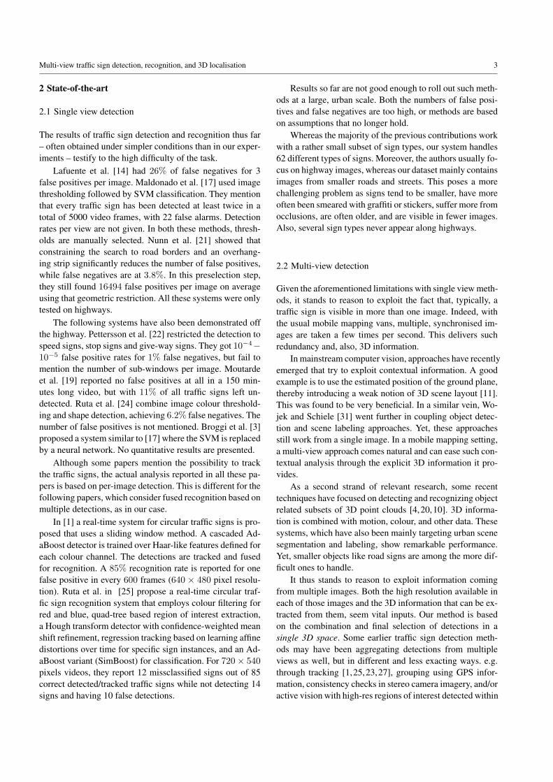
Fig. 3 Haar-like features used in our implementation.

with possible traffic signs. This step requires an automaticoff-line learning stage, where an appropriate subset of fea-tures and corresponding decision rules is selected. They shouldyield very high detection rate (FN very low), while keep-ing the number of false positives in check. This part of thepipeline is described in more detail in Section 4.2) Detection - Extracted candidates are verified further by abinary classifier which filters out remaining background re-gions. It is based on the well known Viola and Jones [30]Discrete AdaBoost classifier [26]. The 6 Haar-like patternsused are shown in Fig. 3. Detection is performed by cas-cades of AdaBoost classifiers, followed by an SVM operat-ing on normalized RGB channels, pyramids of Histogramof Oriented Gradients(HOGs) [2] and AdaBoost-selectedHaar-like features. The detection time is reduced by usingan efficient bounded evaluation of the AdaBoost classifiers,further explained in Section 5.3) Recognition - Six one-against-all SVM classifiers se-lect one of the six basic traffic sign subclasses (triangle-up, triangle-down, circle-blue, circle-red, rectangle and dia-mond) for the different candidate traffic signs. They work onthe RGB colour channels normalized by the intensity vari-ance.

The multi-view phase consists of the following steps:4) Multi-view hypothesis generation - We search for possi-ble correspondences among the final, single-view candidatesin the different views. The search is restricted to a volumewith a predefined radius in 3D space. Every geometricallyand visually consistent pair is used to create a 3D hypothe-sis. Geometric consistency amounts to checking the positionof the back-projected 3D hypothesis against the 2D imagecandidates. Visual consistency gives a higher weight to pairswhich are more probable to be of the same basic shape.5) Multi-view MDL hypothesis pruning - The MinimumDescription Length principle is used to select the subset of3D hypotheses which best explains the overall set of 2D(i.e. single-view) candidates. A by-product of the MDL opti-mization is quite a clean set of 2D candidates correspondingto each particular 3D hypothesis. These candidates allow for3D hypothesis position refinement. Usually, steps 4) and 5)are iterated. More details are given in Section 6.6) Multi-view sign type recognition - The collected set of2D candidates for each 3D hypothesis is classified by anSVM classifier. These classifications then jointly vote on thefinal type assigned to the hypothesis.

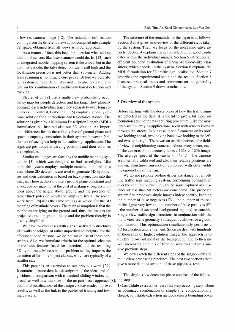
Original Thresholded Connected Extractedimage image I(T ) components bound. boxes

Fig. 4 Colour-based extraction method for threshold T =(0.5, 0.2,−0.4, 1.0)>

Occlusion Occlusion Peeled Dirty

Fig. 5 Not threshold separable traffic signs. There are still trafficsigns which are not well locally separable from background; thereforeshape-based extraction is used.

4 Single-view candidate extraction

The simplest extraction method often used for traffic signdetection is extraction of connected components from a thresh-olded image, an idea already used in [17,3]. The principle isoutlined in Fig. 4. The thresholded image is obtained from acolour image, with colour channels (IR, IG, IB), by appli-cation of a colour threshold T = (t, a, b, c)>:

I(T ) =

{1 a · IR + b · IG + c · IB ≥ t0 otherwise

(1)

Authors often manually select two to five thresholds,which are expected to extract all traffic signs. However, weexperimentally observed that under variable illumination con-ditions and in the presence of a complex background suchextraction method is insufficient.

Since there typically is no single threshold performingwell by itself, it is necessary to combine regions selectedby different thresholds T = {T1, T2, . . . }, in the sense ofadding regions (OR-ing operation). Then, regions passed onby any threshold are going to the next stage, i.e. detection.The more thresholds are used the lower FN can be made butthe higher FP risks to get, and the higher the computationalcost will be.

Partially occluded, peeled or dirty traffic signs also shouldpass the colour test. Therefore, this cannot be made too re-strictive. Examples are shown in Fig. 5. That is why we alsoemploy shape information to further refine the candidates.

Section 4.1 explains how the set of colour thresholdsare learned and how, starting from those, the colour-basedcandidates are extracted. Section 4.2 then describes a shape-based Hough transform. This takes the borders of the colour-based candidates as input.


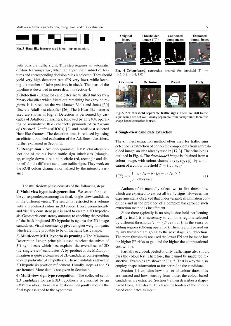
Original Extracted Bounding Rescaledimage region box bound. box

Fig. 6 Demonstration of the extended threshold. The object is notwell locally separable from the background, because bricks have acolour similar to that of the red boundary. Therefore the inner whitepart is extracted and the resulting bounding box is rescaled T =(0.1,−0.433,−0.250, 0.866, 1.6, 1.6)>.

4.1 Colour-based candidate extraction

Given thousands of possible colour thresholds, we search forthe optimal subset T of such thresholds, given some crite-rion. Since for most interesting such criteria the problem isNP-complete, we formulate our search as an Integer LinearProgramming problem. We have experimentally found thatfinding the real optimum takes several hours, but that ILP,due to the sparsity of the constraints, yields a viable solutionwithin minutes.

The most straightforward criterion is to search for a trade-off between FP and FN.

T ∗ = arg minT

(FP(T ) + κ1 · FN(T )), (2)

where FP(T ) stands for the number of false positives andFN(T ) for the number of false negatives, resp., of the se-lected subset of thresholding operations T measured on atraining set. The real number κ1 is a relative weighting fac-tor. In order to avoid overfitting and also to keep the methodsufficiently fast, we introduce an additional constraint on thecardinality card(T ) of the set of selected thresholds. Thiscan be either a hard constraint card(T ) < ω0 or a soft con-straint as in:

T ∗ = arg minT

(FP(T ) + κ1 · FN(T ) + κ2 · card(T )) (3)

We achieved better results with the soft constraint, but im-posing a hard constraint may be necessary if the runningtime is an issue. Since accuracy, defined as the average over-lap between ground truth bounding boxes with extracted bound-ing boxes, is important, we also add a term which increasesthe penalty for inaccurate extractions:

T ∗ = arg minT

(FP(T ) + κ1 · FN(T )

+κ2 · card(T )− κ3 · accuracy(T )) (4)

Scalars κ1, κ2 and κ3 are learned parameters which we esti-mate by cross-validation. Reformulations of problems (2,3,4)into the Integer Linear Programming form are described inthe Appendix.

Original Extracted Hough Refinedimage region accumulator bound. box

Fig. 7 Shape-based extraction principle. The border of the colour-based extracted region (blue) votes for different shapes in a Houghaccumulator. The green bounding box corresponds to the maximum.

Occasionally it happens that the contour of the trafficsign cannot be separated from the background due to coloursimilarity. See for example Fig. 6, where the rim of the signis too similar in colour to the background. Fortunately, manytraffic signs have also some inner contours (e.g. the whiteinner part of the sign in Fig. 6, can be separated rather eas-ily). This inner part can often define the traffic sign’s out-line with sufficient accuracy. We therefore introduce the ex-tended threshold

T = (t, a, b, c︸︷︷︸T

, sr, sc)> (5)

which consists of the original threshold T and vertical resp.horizontal scaling factors (sr, sc) to be applied to the bound-ing box which is extracted with the original threshold. Suchextended threshold - in the sequel simply referred to as thresh-old - can reveal a traffic sign, even if its rim poses problems.

Changing illumination poses another problem to thresh-olding. One could try to adapt the set of thresholds to theillumination conditions, but it is better to add robustness tothe thresholding method itself. We adjust the threshold to belocally stable in the sense of Maximally Stable Extremal Re-gions (MSER) [18]. Instead of directly using the boundingbox as extracted by the learned threshold (t, a, b, c, sr, sc),we use bounding boxes from MSERs detected within therange [(t − ε, a, b, c, sr, sc); (t + ε, a, b, c, sr, sc)], where εis a parameter of the method. Since MSERs themselves aredefined by a stability parameter ∆, this ‘TMSER’ method isparametrized by two parameters (ε,∆).

4.2 Shape-based candidate extraction

Traffic signs are meant to be well distinguishable by boththeir colour and shape. Each of the above thresholds (withscaling and TMSER extensions) let pass a series of con-nected components, i.e. regions (usually thousands per im-age). To these regions we now apply an additional shape-filter, akin to the generalized Hough transformation. Theprinciple is outlined in Fig. 7.

In general the image shapes of the signs will be affinelytransformed versions of the actual shapes. Using the gener-


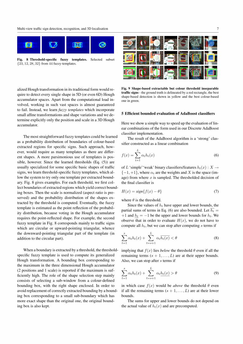
Fig. 8 Threshold-specific fuzzy templates. Selected subset{23, 12, 28, 32} from 44 fuzzy-templates.

alized Hough transformation in its traditional form would re-quire to detect every single shape in 5D (or even 6D) Houghaccumulator spaces. Apart from the computational load in-volved, working in such vast spaces is almost guaranteedto fail. Instead, we learn fuzzy templates which incorporatesmall affine transformations and shape variations and we de-termine explicitly only the position and scale in a 3D Houghaccumulator.

The most straightforward fuzzy templates could be learnedas a probability distribution of boundaries of colour-basedextracted regions for specific signs. Such approach, how-ever, would require as many templates as there are differ-ent shapes. A more parsimonious use of templates is pos-sible, however. Since the learned thresholds (Eq. (5)) areusually specialized for some specific basic shapes of trafficsigns, we learn threshold-specific fuzzy templates, which al-low the system to try only one template per extracted bound-ary. Fig. 8 gives examples. For each threshold, we first col-lect boundaries of extracted regions which yield correct bound-ing boxes. Then the scale is normalized (aspect ratio is pre-served) and the probability distribution of the shapes ex-tracted by the threshold is computed. Eventually, the fuzzytemplate is estimated as the point reflection of the probabil-ity distribution, because voting in the Hough accumulatorrequires the point-reflected shape. For example, the secondfuzzy template in Fig. 8 corresponds mainly to traffic signswhich are circular or upward-pointing triangular, whencethe downward-pointing triangular part of the template (inaddition to the circular part).

When a boundary is extracted by a threshold, the threshold-specific fuzzy template is used to compute its generalizedHough transformation. A bounding box corresponding tothe maximum in the three dimensional Hough accumulator(2 positions and 1 scale) is reported if the maximum is suf-ficiently high. The role of the shape selection step mainlyconsists of selecting a sub-window from a colour-definedbounding box, with the right shape enclosed. In order toavoid replacement of correctly extracted bounding by a bound-ing box corresponding to a small sub-boundary which hasmore exact shape than the original one, the original bound-ing box is also kept.

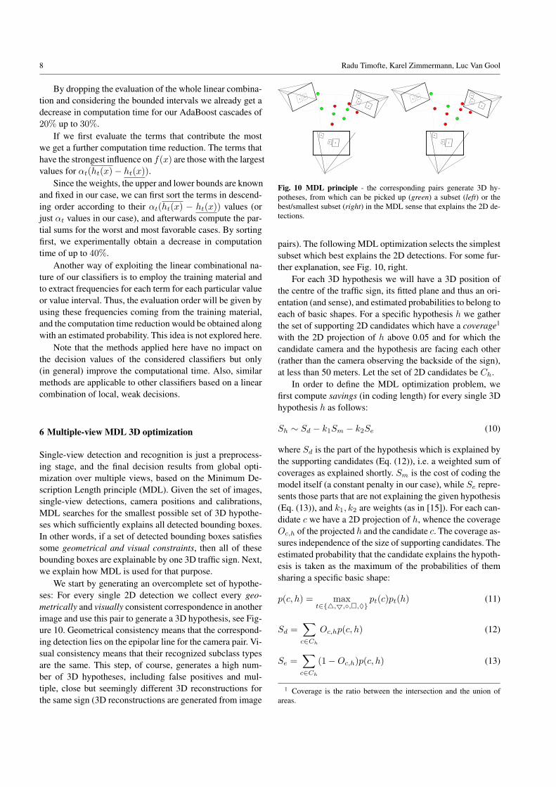
Fig. 9 Shape-based extractable but colour threshold inseparabletraffic signs - the ground truth is delineated by a red rectangle, the bestshape-based detection is shown in yellow and the best colour-basedone in green.

5 Efficient bounded evaluation of AdaBoost classifiers

Here we show a simple way to speed up the evaluation of lin-ear combinations of the form used in our Discrete AdaBoostclassifier implementation.

The result of the AdaBoost algorithm is a ‘strong’ clas-sifier constructed as a linear combination

f(x) =L∑t=1

αtht(x) (6)

of L ‘simple’‘weak’ binary classifiers/features ht(x) : X →{−1,+1}, where αt are the weights andX is the space (im-age) from where x is sampled. The thresholded decision ofthe final classifier is

H(x) = sign{f(x)− θ} (7)

where θ is the threshold.Since the values of ht have upper and lower bounds, the

partial sums of terms in Eq. (6) are also bounded. Let ht =+1 and ht = −1 be the upper and lower bounds for ht. Weobserve that in order to evaluate H(x), we do not have tocompute all ht, but we can stop after computing s terms if

s∑t=1

αtht(x) +L∑

t=s+1

αtht(x) < θ (8)

implying that f(x) lies below the threshold θ even if all theremaining terms (s + 1, . . . , L) are at their upper bounds.Also, we can stop after s terms if

s∑t=1

αtht(x) +L∑

t=s+1

αtht(x) > θ (9)

in which case f(x) would be above the threshold θ evenif all the remaining terms (s + 1, . . . , L) are at their lowerbounds.

The sums for upper and lower bounds do not depend onthe actual value of ht(x) and are precomputed.


By dropping the evaluation of the whole linear combina-tion and considering the bounded intervals we already get adecrease in computation time for our AdaBoost cascades of20% up to 30%.

If we first evaluate the terms that contribute the mostwe get a further computation time reduction. The terms thathave the strongest influence on f(x) are those with the largestvalues for αt(ht(x)− ht(x)).

Since the weights, the upper and lower bounds are knownand fixed in our case, we can first sort the terms in descend-ing order according to their αt(ht(x) − ht(x)) values (orjust αt values in our case), and afterwards compute the par-tial sums for the worst and most favorable cases. By sortingfirst, we experimentally obtain a decrease in computationtime of up to 40%.

Another way of exploiting the linear combinational na-ture of our classifiers is to employ the training material andto extract frequencies for each term for each particular valueor value interval. Thus, the evaluation order will be given byusing these frequencies coming from the training material,and the computation time reduction would be obtained alongwith an estimated probability. This idea is not explored here.

Note that the methods applied here have no impact onthe decision values of the considered classifiers but only(in general) improve the computational time. Also, similarmethods are applicable to other classifiers based on a linearcombination of local, weak decisions.

6 Multiple-view MDL 3D optimization

Single-view detection and recognition is just a preprocess-ing stage, and the final decision results from global opti-mization over multiple views, based on the Minimum De-scription Length principle (MDL). Given the set of images,single-view detections, camera positions and calibrations,MDL searches for the smallest possible set of 3D hypothe-ses which sufficiently explains all detected bounding boxes.In other words, if a set of detected bounding boxes satisfiessome geometrical and visual constraints, then all of thesebounding boxes are explainable by one 3D traffic sign. Next,we explain how MDL is used for that purpose.

We start by generating an overcomplete set of hypothe-ses: For every single 2D detection we collect every geo-metrically and visually consistent correspondence in anotherimage and use this pair to generate a 3D hypothesis, see Fig-ure 10. Geometrical consistency means that the correspond-ing detection lies on the epipolar line for the camera pair. Vi-sual consistency means that their recognized subclass typesare the same. This step, of course, generates a high num-ber of 3D hypotheses, including false positives and mul-tiple, close but seemingly different 3D reconstructions forthe same sign (3D reconstructions are generated from image

Fig. 10 MDL principle - the corresponding pairs generate 3D hy-potheses, from which can be picked up (green) a subset (left) or thebest/smallest subset (right) in the MDL sense that explains the 2D de-tections.

pairs). The following MDL optimization selects the simplestsubset which best explains the 2D detections. For some fur-ther explanation, see Fig. 10, right.

For each 3D hypothesis we will have a 3D position ofthe centre of the traffic sign, its fitted plane and thus an ori-entation (and sense), and estimated probabilities to belong toeach of basic shapes. For a specific hypothesis h we gatherthe set of supporting 2D candidates which have a coverage1

with the 2D projection of h above 0.05 and for which thecandidate camera and the hypothesis are facing each other(rather than the camera observing the backside of the sign),at less than 50 meters. Let the set of 2D candidates be Ch.

In order to define the MDL optimization problem, wefirst compute savings (in coding length) for every single 3Dhypothesis h as follows:

Sh ∼ Sd − k1Sm − k2Se (10)

where Sd is the part of the hypothesis which is explained bythe supporting candidates (Eq. (12)), i.e. a weighted sum ofcoverages as explained shortly. Sm is the cost of coding themodel itself (a constant penalty in our case), while Se repre-sents those parts that are not explaining the given hypothesis(Eq. (13)), and k1, k2 are weights (as in [15]). For each can-didate c we have a 2D projection of h, whence the coverageOc,h of the projected h and the candidate c. The coverage as-sures independence of the size of supporting candidates. Theestimated probability that the candidate explains the hypoth-esis is taken as the maximum of the probabilities of themsharing a specific basic shape:

p(c, h) = maxt∈{4,5,◦,�,♦}

pt(c)pt(h) (11)

Sd =∑c∈Ch

Oc,hp(c, h) (12)

Se =∑c∈Ch

(1−Oc,h)p(c, h) (13)

1 Coverage is the ratio between the intersection and the union ofareas.


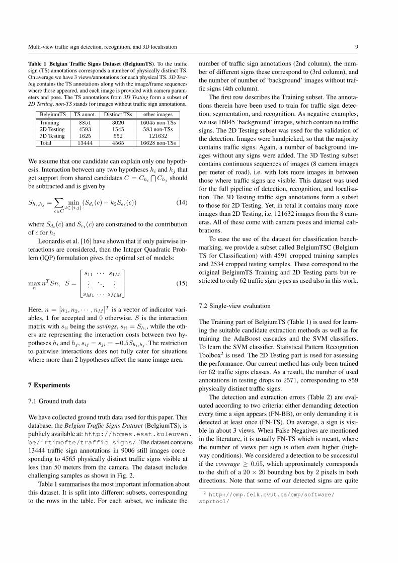
Table 1 Belgian Traffic Signs Dataset (BelgiumTS). To the trafficsign (TS) annotations corresponds a number of physically distinct TS.On average we have 3 views/annotations for each physical TS. 3D Test-ing contains the TS annotations along with the image/frame sequenceswhere those appeared, and each image is provided with camera param-eters and pose. The TS annotations from 3D Testing form a subset of2D Testing. non-TS stands for images without traffic sign annotations.

BelgiumTS TS annot. Distinct TSs other imagesTraining 8851 3020 16045 non-TSs2D Testing 4593 1545 583 non-TSs3D Testing 1625 552 121632Total 13444 4565 16628 non-TSs

We assume that one candidate can explain only one hypoth-esis. Interaction between any two hypotheses hi and hj thatget support from shared candidates C = Chi

⋂Chj should

be subtracted and is given by

Shi,hj=

∑c∈C

mint∈{i,j}

(Sdt(c)− k2Set

(c)) (14)

where Sdt(c) and Set(c) are constrained to the contributionof c for ht

Leonardis et al. [16] have shown that if only pairwise in-teractions are considered, then the Integer Quadratic Prob-lem (IQP) formulation gives the optimal set of models:

maxn

nTSn, S =

s11 · · · s1M.... . .

...sM1 · · · sMM

(15)

Here, n = [n1, n2, · · · , nM ]T is a vector of indicator vari-ables, 1 for accepted and 0 otherwise. S is the interactionmatrix with sii being the savings, sii = Shi

, while the oth-ers are representing the interaction costs between two hy-potheses hi and hj , sij = sji = −0.5Shi,hj . The restrictionto pairwise interactions does not fully cater for situationswhere more than 2 hypotheses affect the same image area.

7 Experiments

7.1 Ground truth data

We have collected ground truth data used for this paper. Thisdatabase, the Belgian Traffic Signs Dataset (BelgiumTS), ispublicly available at: http://homes.esat.kuleuven.be/˜rtimofte/traffic_signs/. The dataset contains13444 traffic sign annotations in 9006 still images corre-sponding to 4565 physically distinct traffic signs visible atless than 50 meters from the camera. The dataset includeschallenging samples as shown in Fig. 2.

Table 1 summarises the most important information aboutthis dataset. It is split into different subsets, correspondingto the rows in the table. For each subset, we indicate the

number of traffic sign annotations (2nd column), the num-ber of different signs these correspond to (3rd column), andthe number of number of ‘background’ images without traf-fic signs (4th column).

The first row describes the Training subset. The annota-tions therein have been used to train for traffic sign detec-tion, segmentation, and recognition. As negative examples,we use 16045 ‘background’ images, which contain no trafficsigns. The 2D Testing subset was used for the validation ofthe detection. Images were handpicked, so that the majoritycontains traffic signs. Again, a number of background im-ages without any signs were added. The 3D Testing subsetcontains continuous sequences of images (8 camera imagesper meter of road), i.e. with lots more images in betweenthose where traffic signs are visible. This dataset was usedfor the full pipeline of detection, recognition, and localisa-tion. The 3D Testing traffic sign annotations form a subsetto those for 2D Testing. Yet, in total it contains many moreimages than 2D Testing, i.e. 121632 images from the 8 cam-eras. All of these come with camera poses and internal cali-brations.

To ease the use of the dataset for classification bench-marking, we provide a subset called BelgiumTSC (BelgiumTS for Classification) with 4591 cropped training samplesand 2534 cropped testing samples. These correspond to theoriginal BelgiumTS Training and 2D Testing parts but re-stricted to only 62 traffic sign types as used also in this work.

7.2 Single-view evaluation

The Training part of BelgiumTS (Table 1) is used for learn-ing the suitable candidate extraction methods as well as fortraining the AdaBoost cascades and the SVM classifiers.To learn the SVM classifier, Statistical Pattern RecognitionToolbox2 is used. The 2D Testing part is used for assessingthe performance. Our current method has only been trainedfor 62 traffic signs classes. As a result, the number of usedannotations in testing drops to 2571, corresponding to 859physically distinct traffic signs.

The detection and extraction errors (Table 2) are eval-uated according to two criteria: either demanding detectionevery time a sign appears (FN-BB), or only demanding it isdetected at least once (FN-TS). On average, a sign is visi-ble in about 3 views. When False Negatives are mentionedin the literature, it is usually FN-TS which is meant, wherethe number of views per sign is often even higher (high-way conditions). We considered a detection to be successfulif the coverage ≥ 0.65, which approximately correspondsto the shift of a 20 × 20 bounding box by 2 pixels in bothdirections. Note that some of our detected signs are quite

2 http://cmp.felk.cvut.cz/cmp/software/stprtool/


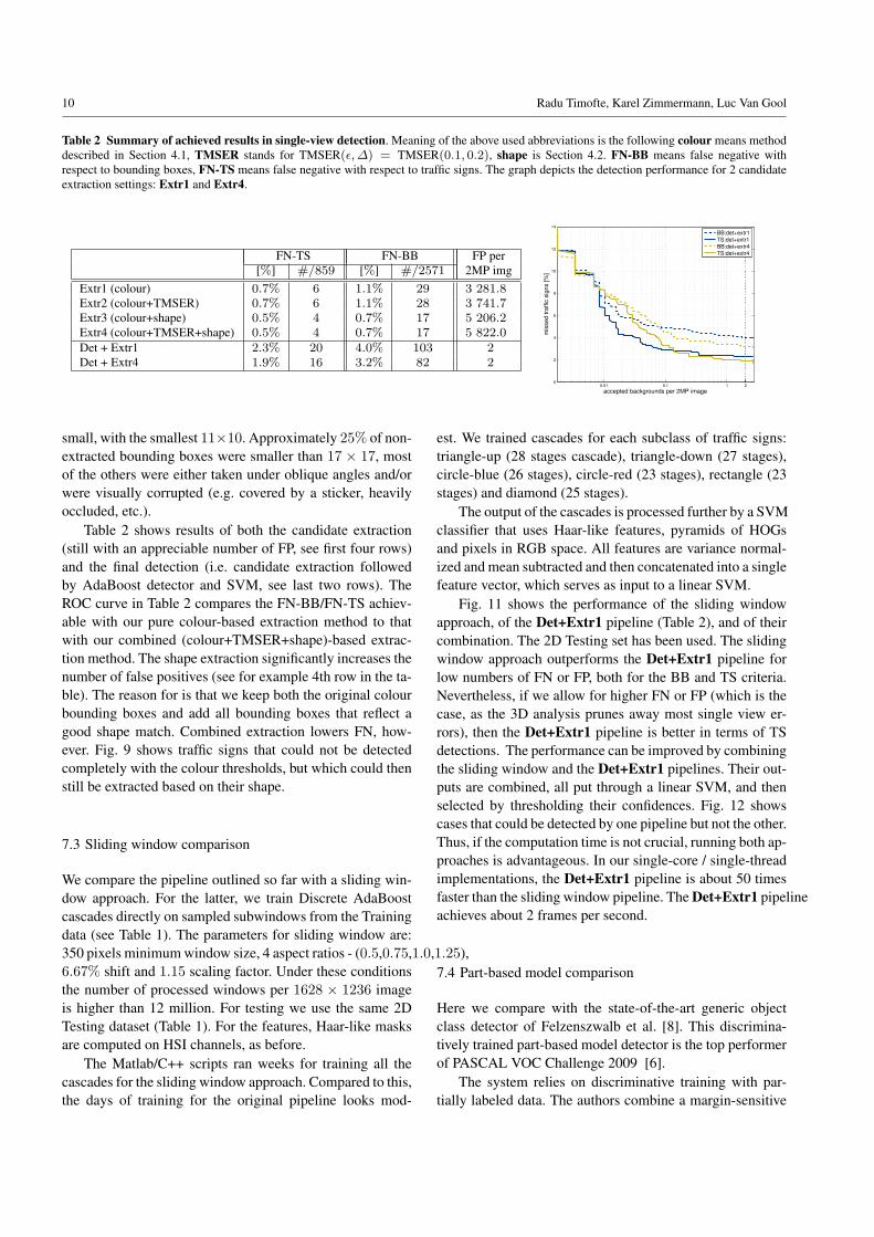
Table 2 Summary of achieved results in single-view detection. Meaning of the above used abbreviations is the following colour means methoddescribed in Section 4.1, TMSER stands for TMSER(ε,∆) = TMSER(0.1, 0.2), shape is Section 4.2. FN-BB means false negative withrespect to bounding boxes, FN-TS means false negative with respect to traffic signs. The graph depicts the detection performance for 2 candidateextraction settings: Extr1 and Extr4.

FN-TS FN-BB FP per[%] #/859 [%] #/2571 2MP img

Extr1 (colour) 0.7% 6 1.1% 29 3 281.8Extr2 (colour+TMSER) 0.7% 6 1.1% 28 3 741.7Extr3 (colour+shape) 0.5% 4 0.7% 17 5 206.2Extr4 (colour+TMSER+shape) 0.5% 4 0.7% 17 5 822.0Det + Extr1 2.3% 20 4.0% 103 2Det + Extr4 1.9% 16 3.2% 82 2

0.01 0.1 1 20

2

4

6

8

10

12

14

accepted backgrounds per 2MP image

mis

sed tra

ffic

sig

ns [%

]

BB:det+extr1

TS:det+extr1

BB:det+extr4

TS:det+extr4

small, with the smallest 11×10. Approximately 25% of non-extracted bounding boxes were smaller than 17 × 17, mostof the others were either taken under oblique angles and/orwere visually corrupted (e.g. covered by a sticker, heavilyoccluded, etc.).

Table 2 shows results of both the candidate extraction(still with an appreciable number of FP, see first four rows)and the final detection (i.e. candidate extraction followedby AdaBoost detector and SVM, see last two rows). TheROC curve in Table 2 compares the FN-BB/FN-TS achiev-able with our pure colour-based extraction method to thatwith our combined (colour+TMSER+shape)-based extrac-tion method. The shape extraction significantly increases thenumber of false positives (see for example 4th row in the ta-ble). The reason for is that we keep both the original colourbounding boxes and add all bounding boxes that reflect agood shape match. Combined extraction lowers FN, how-ever. Fig. 9 shows traffic signs that could not be detectedcompletely with the colour thresholds, but which could thenstill be extracted based on their shape.

7.3 Sliding window comparison

We compare the pipeline outlined so far with a sliding win-dow approach. For the latter, we train Discrete AdaBoostcascades directly on sampled subwindows from the Trainingdata (see Table 1). The parameters for sliding window are:350 pixels minimum window size, 4 aspect ratios - (0.5,0.75,1.0,1.25),6.67% shift and 1.15 scaling factor. Under these conditionsthe number of processed windows per 1628 × 1236 imageis higher than 12 million. For testing we use the same 2DTesting dataset (Table 1). For the features, Haar-like masksare computed on HSI channels, as before.

The Matlab/C++ scripts ran weeks for training all thecascades for the sliding window approach. Compared to this,the days of training for the original pipeline looks mod-

est. We trained cascades for each subclass of traffic signs:triangle-up (28 stages cascade), triangle-down (27 stages),circle-blue (26 stages), circle-red (23 stages), rectangle (23stages) and diamond (25 stages).

The output of the cascades is processed further by a SVMclassifier that uses Haar-like features, pyramids of HOGsand pixels in RGB space. All features are variance normal-ized and mean subtracted and then concatenated into a singlefeature vector, which serves as input to a linear SVM.

Fig. 11 shows the performance of the sliding windowapproach, of the Det+Extr1 pipeline (Table 2), and of theircombination. The 2D Testing set has been used. The slidingwindow approach outperforms the Det+Extr1 pipeline forlow numbers of FN or FP, both for the BB and TS criteria.Nevertheless, if we allow for higher FN or FP (which is thecase, as the 3D analysis prunes away most single view er-rors), then the Det+Extr1 pipeline is better in terms of TSdetections. The performance can be improved by combiningthe sliding window and the Det+Extr1 pipelines. Their out-puts are combined, all put through a linear SVM, and thenselected by thresholding their confidences. Fig. 12 showscases that could be detected by one pipeline but not the other.Thus, if the computation time is not crucial, running both ap-proaches is advantageous. In our single-core / single-threadimplementations, the Det+Extr1 pipeline is about 50 timesfaster than the sliding window pipeline. The Det+Extr1 pipelineachieves about 2 frames per second.

7.4 Part-based model comparison

Here we compare with the state-of-the-art generic objectclass detector of Felzenszwalb et al. [8]. This discrimina-tively trained part-based model detector is the top performerof PASCAL VOC Challenge 2009 [6].

The system relies on discriminative training with par-tially labeled data. The authors combine a margin-sensitive


0.01 0.1 1 20

2

4

6

8

10

12

14

accepted backgrounds per 2MP image

mis

sed tra

ffic

sig

ns [%

]

BB:det+extr1

TS:det+extr1

BB:sliding window

TS:sliding window

BB:combined (sliding window & det+extr1)

TS:combined (sliding window & det+extr1)

BB:part−based models (Felzenszwalb)

TS:part−based models (Felzenszwalb)

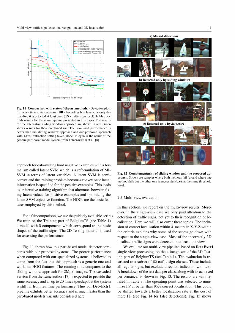
Fig. 11 Comparison with state-of-the-art methods. - Detection plotsfor every time a sign appears (BB - bounding box level), or only de-manding it is detected at least once (TS - traffic sign level). In blue onefinds results for the main pipeline presented in this paper. The resultsfor the alternative sliding window approach are shown in red. Greenshows results for their combined use. The combined performance isbetter than the sliding window approach and our proposed approachwith Extr1 extraction setting taken alone. In cyan is the result of thegeneric part-based model system from Felzenszwalb et al. [8]

approach for data-mining hard negative examples with a for-malism called latent SVM which is a reformulation of MI-SVM in terms of latent variables. A latent SVM is semi-convex and the training problem becomes convex once latentinformation is specified for the positive examples. This leadsto an iterative training algorithm that alternates between fix-ing latent values for positive examples and optimizing thelatent SVM objective function. The HOGs are the basic fea-tures employed by this method.

For a fair comparison, we use the publicly available scripts.We train on the Training part of BelgiumTS (see Table 1)a model with 5 components which correspond to the basicshapes of the traffic signs. The 2D Testing material is usedfor assessing the performance.

Fig. 11 shows how this part-based model detector com-pares with our proposed systems. The poorer performancewhen compared with our specialized systems is believed tocome from the fact that this approach is a generic one andworks on HOG features. The running time compares to thesliding window approach for 2Mpxl images. The cascadedversion from the same authors [7] is expected to provide thesame accuracy and an up to 20 times speedup, but the systemis still far from realtime performance. Thus our Det+Extr1pipeline exhibits better accuracy and is much faster than thepart-based models variants considered here.

a) Missed detections:

b) Detected only by sliding window:

c) Detected only by det+extr1:

Fig. 12 Complementarity of sliding window and the proposed ap-proach. Shown are samples where both methods fail (a) and where onemethod fails but the other one is successful (b,c), at the same thresholdlevel.

7.5 Multi-view evaluation

In this section, we report on the multi-view results. More-over, in the single-view case we only paid attention to thedetection of traffic signs, not yet to their recognition or lo-calisation. Here we will also cover these topics. The inclu-sion of correct localisation within 3 meters in X-Y-Z withinthe criteria explains why some of the scores go down withrespect to the single-view case. Most of the incorrectly 3Dlocalised traffic signs were detected in at least one view.

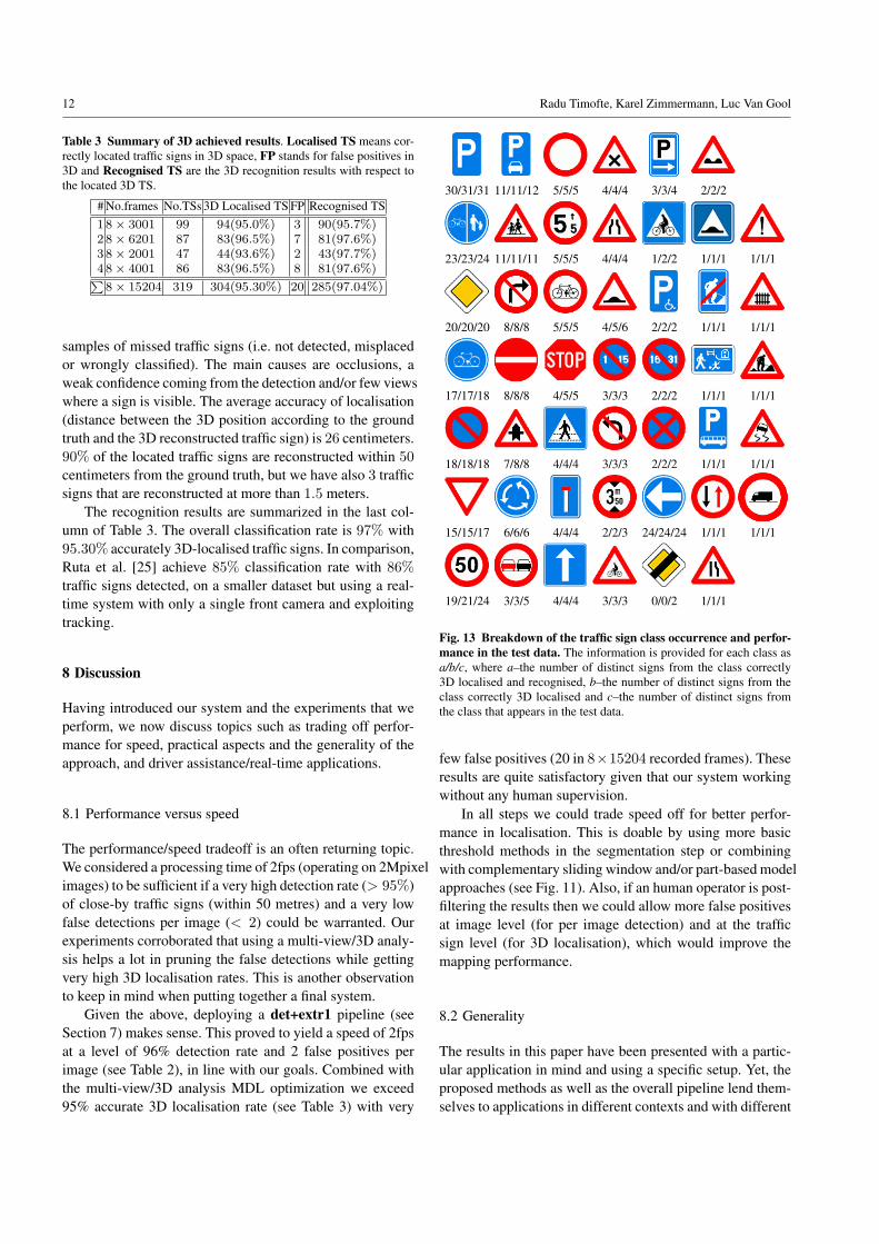
We evaluate our multi-view pipeline, based on Det+Extr1single-view processing, on the 4 image sets of the 3D Test-ing part of BelgiumTS (see Table 1). The evaluation is re-stricted to a subset of 62 traffic sign classes. These includeall regular signs, but exclude direction indicators with text.A breakdown of the test data per class, along with its achievedperformance, is shown in Fig. 13. The results are summa-rized in Table 3. The operating point was selected to mini-mize FP at better than 95% correct localisation. This couldbe shifted towards a better localisation rate at the cost ofmore FP (see Fig. 14 for false detections). Fig. 15 shows


Table 3 Summary of 3D achieved results. Localised TS means cor-rectly located traffic signs in 3D space, FP stands for false positives in3D and Recognised TS are the 3D recognition results with respect tothe located 3D TS.

# No.frames No.TSs 3D Localised TS FP Recognised TS18× 3001 99 94(95.0%) 3 90(95.7%)28× 6201 87 83(96.5%) 7 81(97.6%)38× 2001 47 44(93.6%) 2 43(97.7%)48× 4001 86 83(96.5%) 8 81(97.6%)P8× 15204 319 304(95.30%) 20 285(97.04%)

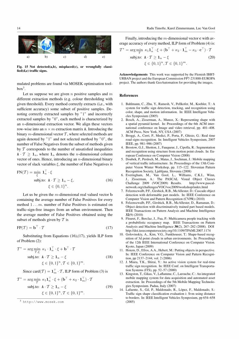
samples of missed traffic signs (i.e. not detected, misplacedor wrongly classified). The main causes are occlusions, aweak confidence coming from the detection and/or few viewswhere a sign is visible. The average accuracy of localisation(distance between the 3D position according to the groundtruth and the 3D reconstructed traffic sign) is 26 centimeters.90% of the located traffic signs are reconstructed within 50centimeters from the ground truth, but we have also 3 trafficsigns that are reconstructed at more than 1.5 meters.

The recognition results are summarized in the last col-umn of Table 3. The overall classification rate is 97% with95.30% accurately 3D-localised traffic signs. In comparison,Ruta et al. [25] achieve 85% classification rate with 86%traffic signs detected, on a smaller dataset but using a real-time system with only a single front camera and exploitingtracking.

8 Discussion

Having introduced our system and the experiments that weperform, we now discuss topics such as trading off perfor-mance for speed, practical aspects and the generality of theapproach, and driver assistance/real-time applications.

8.1 Performance versus speed

The performance/speed tradeoff is an often returning topic.We considered a processing time of 2fps (operating on 2Mpixelimages) to be sufficient if a very high detection rate (> 95%)of close-by traffic signs (within 50 metres) and a very lowfalse detections per image (< 2) could be warranted. Ourexperiments corroborated that using a multi-view/3D analy-sis helps a lot in pruning the false detections while gettingvery high 3D localisation rates. This is another observationto keep in mind when putting together a final system.

Given the above, deploying a det+extr1 pipeline (seeSection 7) makes sense. This proved to yield a speed of 2fpsat a level of 96% detection rate and 2 false positives perimage (see Table 2), in line with our goals. Combined withthe multi-view/3D analysis MDL optimization we exceed95% accurate 3D localisation rate (see Table 3) with very

30/31/31

23/23/24

20/20/20

17/17/18

18/18/18

15/15/17

19/21/24

11/11/12

11/11/11

8/8/8

8/8/8

7/8/8

6/6/6

3/3/5

5/5/5

5/5/5

5/5/5

4/5/5

4/4/4

4/4/4

4/4/4

4/4/4

4/4/4

4/5/6

3/3/3

3/3/3

2/2/3

3/3/3

3/3/4

1/2/2

2/2/2

2/2/2

2/2/2

24/24/24

0/0/2

2/2/2

1/1/1

1/1/1

1/1/1

1/1/1

1/1/1

1/1/1

1/1/1

1/1/1

1/1/1

1/1/1

1/1/1

Fig. 13 Breakdown of the traffic sign class occurrence and perfor-mance in the test data. The information is provided for each class asa/b/c, where a–the number of distinct signs from the class correctly3D localised and recognised, b–the number of distinct signs from theclass correctly 3D localised and c–the number of distinct signs fromthe class that appears in the test data.

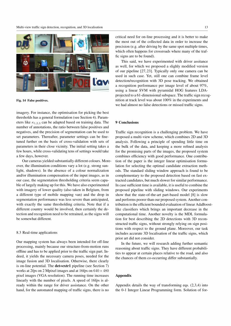
few false positives (20 in 8×15204 recorded frames). Theseresults are quite satisfactory given that our system workingwithout any human supervision.

In all steps we could trade speed off for better perfor-mance in localisation. This is doable by using more basicthreshold methods in the segmentation step or combiningwith complementary sliding window and/or part-based modelapproaches (see Fig. 11). Also, if an human operator is post-filtering the results then we could allow more false positivesat image level (for per image detection) and at the trafficsign level (for 3D localisation), which would improve themapping performance.

8.2 Generality

The results in this paper have been presented with a partic-ular application in mind and using a specific setup. Yet, theproposed methods as well as the overall pipeline lend them-selves to applications in different contexts and with different


Fig. 14 False positives.

imagery. For instance, the optimisation for picking the bestthresholds has a general formulation (see Section 4). Param-eters like κ1,2,3 can be adapted based on training data. Thenumber of annotations, the ratio between false positives andnegatives, and the precision of segmentation can be used toset parameters. Thereafter, parameter settings can be fine-tuned further on the basis of cross-validation with sets ofparameters in their close vicinity. The initial setting takes afew hours, while cross-validating tens of settings would takea few days, however.

Our cameras yielded substantially different colours. More-over, the illumination conditions vary a lot (e.g. strong sun-light, shadows). In the absence of a colour normalizationand/or illumination compensation of the input images, as inour case, the segmentation thresholding criteria seem capa-ble of largely making up for this. We have also experimentedwith imagery of lower quality (also taken in Belgium, froma different type of mobile mapping van) and the drop insegmentation performance was less severe than anticipated,with exactly the same thresholding criteria. Note that if adifferent country would be involved, then certainly the de-tection and recognition need to be retrained, as the signs willbe somewhat different.

8.3 Real-time applications

Our mapping system has always been intended for off-lineprocessing, mainly because our structure-from-motion runsoffline and has to be applied prior to the traffic sign part. In-deed, it yields the necessary camera poses, needed for theimage fusion and 3D localisation. Otherwise, there clearlyis on-line potential. The det+extr1 pipeline (see Section 7)works at 2fps on 2 Mpixel images and at 16fps on 640×480pixel images (VGA resolution). The running time increaseslinearly with the number of pixels. A speed of 16fps is al-ready within the range for driver assistance. On the otherhand, for the automated mapping of traffic signs, there is no

critical need for on-line processing and it is better to makethe most out of the collected data in order to increase theprecision (e.g. after driving by the same spot multiple times,which often happens for crossroads where many of the traf-fic signs are to be found).

This said, we have experimented with driver assitanceas well, for which we proposed a slighly modified versionof our pipeline [27,23]. Typically only one camera can beused in such case. Yet, still one can combine frame leveldetection/recognition with 3D pose tracking. We obtaineda recognition performance per image level of about 97%,using a linear SVM with pyramidal HOG features LDA-projected to a 61-dimensional subspace. The traffic sign recog-nition at track level was about 100% in the experiments andwe had almost no false detections or missed traffic signs.

9 Conclusions

Traffic sign recognition is a challenging problem. We haveproposed a multi-view scheme, which combines 2D and 3Danalysis. Following a principle of spending little time onthe bulk of the data, and keeping a more refined analysisfor the promising parts of the images, the proposed systemcombines efficiency with good performance. One contribu-tion of the paper is the integer linear optimisation formu-lation for selecting the optimal candidate extraction meth-ods. The standard sliding window approach is found to becomplementary to the proposed detection based on fast ex-tracted candidates, but much slower for similar performance.In case sufficient time is available, it is useful to combine theproposed pipeline with sliding windows. Our experimentsshow that the state-of-the-art part-based model [8] is slowand performs poorer than our proposed system. Another con-tribution is the efficient bounded evaluation of linear AdaBoost-like classifiers which brings an important decrease in thecomputational time. Another novelty is the MDL formula-tion for best describing the 2D detections with 3D recon-structed traffic signs, without strongly relying on sign posi-tions with respect to the ground plane. Moreover, our taskincludes accurate 3D localisation of the traffic signs, whichprior art did not consider.

In the future, we will research adding further semanticreasoning about traffic signs. They have different probabili-ties to appear at certain places relative to the road, and alsothe chances of them co-occurring differ substantially.

Appendix

Appendix details the way of transforming eqs. (2,3,4) intothe 0-1 Integer Linear Programming form. Solution of for-


a) b) c) d) e)

Fig. 15 Not detected(a,b), misplaced(c), or wrongfully classi-fied(d,e) traffic signs.

mulated problems are found via MOSEK optimisation tool-box3.

Let us suppose we are given n positive samples and mdifferent extraction methods (e.g. colour thresholding withgiven threshold). Every method correctly extracts (i,e., withsufficient accuracy) some subset of positive samples. De-noting correctly extracted samples by ”1” and incorrectlyextracted samples by ”0”, each method is characterized byan n-dimensional extraction vector. We align these vectorsrow-wise into an n×m extraction matrix A. Introducing thebinarym-dimensional vector T , where selected methods areagain denoted by ”1” and not selected method by ”0”, thenumber of False Negatives from the subset of methods givenby T corresponds to the number of unsatisfied inequalitiesA · T ≥ 1n, where 1n denotes the n-dimensional columnvector of ones. Hence, introducing an n-dimensional binaryvector of slack variables ξ, the number of False Negatives is

FN(T ) = minξ

1>n · ξ

subj.to: A · T ≥ 1n − ξ, (16)

ξ ∈ {0, 1}n.

Let us be given the m-dimensional real valued vector bcontaining the average number of False Positives for everymethod 1 . . .m. number of False Positives is estimated ontraffic-sign-free images from an urban environment. Thenthe average number of False Positives obtained using thesubset of methods given by T is

FP(T ) = b> · T (17)

Substituting from Equations (16),(17), yields ILP formof Problem (2):

T ∗ = arg minT ,ξ

κ1 · 1>n · ξ + b> · T

subj.to: A · T ≥ 1n − ξ (18)

ξ ∈ {0, 1}n, T ∈ {0, 1}m.

Since card(T ) = 1>m · T , ILP form of Problem (3) is

T ∗ = arg minT

κ11>n · ξ + (b> + κ2 · 1>m) · T

subj.to: A · T ≥ 1n − ξ (19)

ξ ∈ {0, 1}n, T ∈ {0, 1}m.

3 http://www.mosek.com

Finally, introducing them-dimensional vector c with av-erage accuracy of every method, ILP form of Problem (4) is:

T ∗ = arg minT

κ11>n · ξ + (b> + κ2 · 1>m − κ3 · c>) · T

subj.to: A · T ≥ 1n − ξ (20)

ξ ∈ {0, 1}n, T ∈ {0, 1}m.

Acknowledgements This work was supported by the Flemish IBBT-URBAN project and the European Commission FP7-231888-EUROPAproject. The authors thank GeoAutomation for providing the images.

References

1. Bahlmann, C., Zhu, Y., Ramesh, V., Pellkofer, M., Koehler, T.: Asystem for traffic sign detection, tracking, and recognition usingcolor, shape, and motion information. In: IEEE Intelligent Vehi-cles Symposium (2005)

2. Bosch, A., Zisserman, A., Munoz, X.: Representing shape witha spatial pyramid kernel. In: Proceedings of the 6th ACM inter-national conference on Image and video retrieval, pp. 401–408.ACM Press, New York, NY, USA (2007)

3. Broggi, A., Cerri, P., Medici, P., Porta, P., Ghisio, G.: Real timeroad signs recognition. In: Intelligent Vehicles Symposium, 2007IEEE, pp. 981–986 (2007)

4. Brostow, G.J., Shotton, J., Fauqueur, J., Cipolla, R.: Segmentationand recognition using structure from motion point clouds. In: Eu-ropean Conference on Computer Vision (2008)

5. Doubek, P., Perdoch, M., Matas, J., Sochman, J.: Mobile mappingof vertical traffic infrastructure. In: Proceedings of the 13th Com-puter Vision Winter Workshop, pp. 115–122. Slovenian PatternRecognition Society, Ljubljana, Slovenia (2008)

6. Everingham, M., Van Gool, L., Williams, C.K.I., Winn,J., Zisserman, A.: The PASCAL Visual Object ClassesChallenge 2009 (VOC2009) Results. http://www.pascal-network.org/challenges/VOC/voc2009/workshop/index.html

7. Felzenszwalb, P.F., Girshick, R.B., McAllester, D.: Cascade objectdetection with deformable part models. In: IEEE Conference onComputer Vision and Pattern Recognition (CVPR) (2010)

8. Felzenszwalb, P.F., Girshick, R.B., McAllester, D., Ramanan, D.:Object detection with discriminatively trained part based models.IEEE Transactions on Pattern Analysis and Machine Intelligence32(9) (2010)

9. Fleuret, F., Berclaz, J., Fua, P.: Multicamera people tracking witha probabilistic occupancy map. IEEE Transactions on PatternAnalysis and Machine Intelligence 30(2), 267–282 (2008). DOIhttp://doi.ieeecomputersociety.org/10.1109/TPAMI.2007.1174

10. Golovinskiy, A., Kim, V.G., Funkhouser, T.: Shape-based recog-nition of 3d point clouds in urban environments. In: Proceedingsof the 12th IEEE International Conference on Computer Vision.Kyoto, Japan (2009)

11. Hoiem, D., Efros, A.A., Hebert, M.: Putting objects in perspective.In: IEEE Conference on Computer Vision and Pattern Recogni-tion, pp 2137–2144, vol. 2 (2006)

12. J. Miura, T.K., Shirai, Y.: An active vision system for real-timetraffic sign recognition. In: IEEE Conf. on Intelligent Transporta-tion Systems (ITS), pp. 52–57 (2000)

13. Kingston, T., Gikas, V., Laflamme, C., Larouche, C.: An integratedmobile mapping system for data acquisition and automated assetextraction. In: Proceedings of the 5th Mobile Mapping Technolo-gies Symposium. Padua, Italy (2007)

14. Lafuente, S., Gil, P., Maldonado, R., Lopez, F., Maldonado, S.:Traffic sign shape classification evaluation i: Svm using distanceto borders. In: IEEE Intelligent Vehicles Symposium, pp 654–658(2005)


15. Leibe, B., Schindler, K., Cornelis, N., Van Gool, L.: Coupled ob-ject detection and tracking from static cameras and moving vehi-cles. IEEE Transactions on Pattern Analysis and Machine Intelli-gence 30(10), 1683–1698 (2008)

16. Leonardis, A., Gupta, A., Bajcsy, R.: Segmentation of range im-ages as the search for geometric parametric models. InternationalJournal of Computer Vision, pp 253–277 14(3) (1995)

17. Maldonado, S., Lafuente, S., Gil, P., Gomez, H., Lopez, F.: Road-sign detection and recognition based on support vector machines.IEEE Trans. Intelligent Transportation Systems, pp 264–278 8(2)(2007)

18. Matas, J., Chum, O., Urban, M., Pajdla, T.: Robust wide baselinestereo from maximally stable extremal regions. In: British Ma-chine Vision Conference, pp 384-393, vol. 1 (2002)

19. Moutarde, F., Bargeton, A., Herbin, A., Chanussot, L.: Robust on-vehicle real-time visual detection of american and european speedlimit signs, with a modular traffic signs recognition system. In:IEEE Intelligent Vehicles Symposium, pp 1122–1126 (2007)

20. Munoz, D., Vandapel, N., Hebert, M.: Directional associativemarkov network for 3-d point cloud classification. In: 3D DataProcessing Visualization and Transmission (2008)

21. Nunn, C., Kummert, A., Muller-Schneiders, S.: A novel region ofinterest selection approach for traffic sign recognition based on 3dmodelling. In: IEEE Intelligent Vehicles Symposium, pp 654–658(2008)

22. Pettersson, N., Petersson, L., Andersson, L.: The histogram fea-ture - a resource-efficient weak classifier. In: IEEE Intelligent Ve-hicles Symposium, pp 678 - 683 (2008)

23. Prisacariu, V.A., Timofte, R., Zimmermann, K., Reid, I., VanGool, L.J.: Integrating object detection with 3d tracking towards abetter driver assistance system. In: 20th International Conferenceon Pattern Recognition, ICPR 2010, Istanbul, Turkey, pp. 3344–3347 (2010)

24. Ruta, A., Li, Y., Liu, X.: Towards real-time traffic sign recogni-tion by class-specific discriminative features. In: British MachineVision Conference (2007)

25. Ruta, A., Porikli, F., Watanabe, S., Li, Y.: In-vehicle camera trafficsign detection and recognition. Mach. Vis. Appl. 22(2), 359–375(2011)

26. Schapire, R.E., Freund, Y., Bartlett, P., Lee, W.S.: Boosting themargin: a new explanation for the effectiveness of voting methods.The Annals of Statistics 26(5), 1651–1686 (1998)

27. Timofte, R., Prisacariu, V.A., Van Gool, L.J., Reid, I.: Chapter3.5: Combining traffic sign detection with 3d tracking towardsbetter driver assistance. In: C.H. Chen (ed.) Emerging Topics inComputer Vision and its Applications. World Scientific Publishing(2011)

28. Timofte, R., Van Gool, L.: Multi-view manhole detection, recogni-tion, and 3d localisation. In: 1st IEEE/ISPRS Workshop on Com-puter Vision for Remote Sensing of the Environment (CVRS) inconjunction with the 13th International Conference on ComputerVision (ICCV) (2011)

29. Timofte, R., Zimmermann, K., Van Gool, L.: Multi-view trafficsign detection, recognition, and 3d localisation. In: Proceedings ofthe IEEE Computer Society’s Workshop on Applications of Com-puter Vision (WACV). IEEE Computer Society, Snowbird, Utah,USA (2009)

30. Viola, P., Jones, M.: Robust real-time face detection. In: IEEEInternational Conference on Computer Vision, vol. 2, pp. 747–757(2001)

31. Wojek, C., Schiele, B.: A dynamic conditional random field modelfor joint labeling of object and scene classes. In: European Con-ference on Computer Vision, pp 733-747 (2008)

Documents

Multi-view trafﬁc sign detection, recognition, and 3D ...timofter/publications/Timofte-MVA-2011... · Multi-view trafﬁc sign detection, recognition, and 3D localisation ... Keywords