Fall 2012

Directed by : Dr. Darhmaoui

Physics 1402 :

Final Project

RLC Circuit

Zdadou Fatima Ezzahra & Derj Atar

1 | P a g e

Introduction:

R, L and C are the basic passive elements in electric and electronic

circuit their combination in series or in parallel could serve as a

hardware function.

The purpose of this project is to study the behavior of those elements by

combining them in a circuit which is called RLC circuit, and to get a

response of frequency.

To study the behavior, we divide the project in 3 mainly parts which are:

The theoretical part,

The simulation part,

And the experimental part.

2 | P a g e

An RLC circuit (or LCR circuit) is an electrical circuit consisting of a resistor, an inductor, and

a capacitor, connected in series or in parallel. The RLC part of the name is due to those letters

being the usual electrical symbols for resistance, inductance and capacitance respectively.

Resistor:

A resistor is a passive two-terminal electrical component that implements electrical resistance as

a circuit element.

The current through a resistor is in direct proportion to the voltage across the resistor's terminals.

This relationship is represented by Ohm's law: I= V/R

where I is the current through the conductor in units of amperes, V is the potential difference

measured across the conductor in units of volts, and R is the resistance of the conductor in units

of ohms.

Inductance:

An inductor (also choke, coil or reactor) is a passive two-terminal electrical component that

stores energy in its magnetic field. For comparison, a capacitor stores energy in an electric field,

and a resistor does not store energy but rather dissipates energy as heat.

Capacitance:

A capacitance is the ability of a body to store an electrical charge. Any body or structure that is

capable of being charged, either with static electricity or by an electric current, exhibits

capacitance. A common form of energy storage device is a parallel-plate capacitor. In a parallel

plate capacitor, capacitance is directly proportional to the surface area of the conductor plates

and inversely proportional to the separation distance between the plates. If the charges on the

plates are +q and −q, and V gives the voltage between the plates, then the capacitance C is given

by C= q/V.

The capacitance is a function only of the physical dimensions (geometry) of the conductors and

the permittivity of the dielectric. It is independent of the potential difference between the

conductors and the total charge on them.

3 | P a g e

1st Part (In Series):

A. Circuit Analysis:

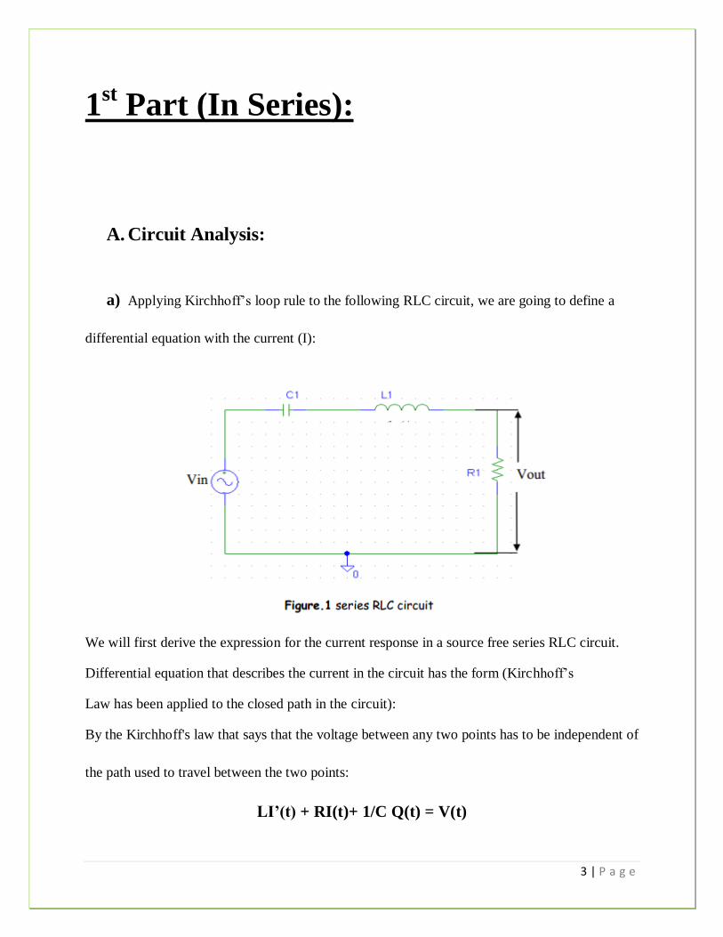
a) Applying Kirchhoff’s loop rule to the following RLC circuit, we are going to define a

differential equation with the current (I):

We will first derive the expression for the current response in a source free series RLC circuit.

Differential equation that describes the current in the circuit has the form (Kirchhoff’s

Law has been applied to the closed path in the circuit):

By the Kirchhoff's law that says that the voltage between any two points has to be independent of

the path used to travel between the two points:

LI’(t) + RI(t)+ 1/C Q(t) = V(t)

4 | P a g e

Assuming that R; L; C and V are known, this is still one differential equation in two unknowns, I

and Q. However the two unknowns are related by:

I(t) = dQ(t) /dt

So, that :

LQ’’(t) + RQ’(t) +

Q(t) = V(t)

or, differentiating with respect to t and then subbing in:

(t) = I(t)

Then we replace it, we result with:

LI’’ (t) + RI’+

I(t) = V’(t)

For an ac voltage source, choosing the origin of time so that:

V(0) = 0 , V(t) = E0sin(wt)

and the final differential equation becomes:

LI’’(t) + RI’(t) +

I(t) = wE0cos(wt)

b) Assuming that at t=0 (when the switch is closed), I = 0 & (d/dt)I = 0, we are going to

solve the differential equation to find the function(s) for the current in the circuit :

We take the previous result that we got – the differential equation- :

5 | P a g e

LI’’(t) + RI’(t) +

I(t) = wE0cos(wt) (1)

Now, we guess one solution of this equation by trying :

Ip (t) = A sin (wt - φ ) (2)

With A= Amplitude , φ = Phase (To be determined)

We plug (2) in (1):

L Ip’’(t) + R Ip’(t) +

Ip (t) = wE0cos(wt)

-Lw²Asin(wt - φ)+RwAcos(wt - φ)+

Asin(wt - φ)= wE0cos(wt)

= wE0cos(wt- φ + φ )

Then:

(1/C-Lw²)Asin(wt - φ )+RwAcos(wt - φ )=wE0cos(φ)cos(wt - φ)-wE0sin(φ) sin(wt - φ)

So,

(Lw² -

)A = wE0sin(φ) (3)

RwA = wE0cos(φ) (4)

Now, we solve for A and φ :

To calculate φ :

(3)/(4)

tan(φ) =

φ = tan ^-1 (

)

To calculate A:

6 | P a g e

√((Lw²-1/C)²+R²w²A) = wE0

A = wE0 / √((Lw²-1/C)²+R²w²A)

= E0 / √((Lw-1/Cw)²+R²)

At t= 0:

A= Imax & impedance Z=

So, Imax = E0 / Z

If the capacitive reactance is greater than the inductive reactance: Xc > Xl then the overall circuit

reactance is capacitive giving a leading phase angle. Likewise, if the inductive reactance is

greater than the capacitive reactance, XL > XC then the overall circuit reactance is inductive

giving the series circuit a lagging phase angle. If the two reactance's are the same

and XL = XC then the angular frequency at which this occurs is called the resonant frequency and

produces the effect of resonance. Therefore, it is a good filter at this resonant frequency.

Then the magnitude of the current depends upon the frequency applied to the series RLC circuit.

When impedance, Z is at its maximum, the current is a minimum and likewise, when Z is at its

minimum, the current is at maximum.

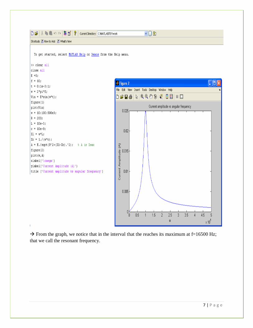
c) To solve the differential equation and plot the current magnitude vs. frequency, we used

MatLab (Version 7):

Given the following values:

R = 200 ohms Vin (t) = 5.0 sin (ωt) volts, L = 10 mHenry, C =10 nFarads

We will add them to proceed by having our differents plots:

7 | P a g e

From the graph, we notice that in the interval that the reaches its maximum at f=16500 Hz;

that we call the resonant frequency.

8 | P a g e

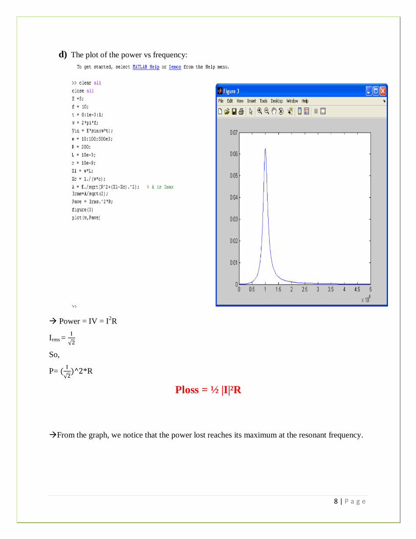
d) The plot of the power vs frequency:

Power = IV = I2R

Irms =

So,

P=

*R

Ploss = ½ |I|²R

From the graph, we notice that the power lost reaches its maximum at the resonant frequency.

9 | P a g e

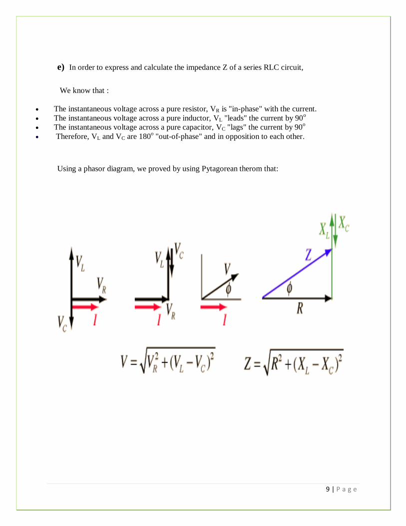
e) In order to express and calculate the impedance Z of a series RLC circuit,

We know that :

The instantaneous voltage across a pure resistor, VR is "in-phase" with the current.

The instantaneous voltage across a pure inductor, VL "leads" the current by 90o

The instantaneous voltage across a pure capacitor, VC "lags" the current by 90o

Therefore, VL and VC are 180o "out-of-phase" and in opposition to each other.

Using a phasor diagram, we proved by using Pytagorean therom that:

10 | P a g e

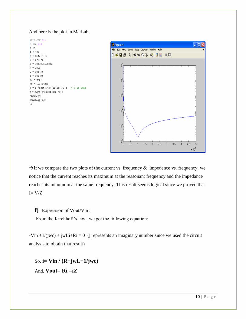
And here is the plot in MatLab:

If we compare the two plots of the current vs. frequency & impedence vs. frequency, we

notice that the current reaches its maximum at the reasonant frequency and the impedance

reaches its minumum at the same frequency. This result seems logical since we proved that

I= V/Z.

f) Expression of Vout/Vin :

From the Kirchhoff’s law, we got the following equation:

-Vin + i/(jwc) + jwLi+Ri = 0 (j represents an imaginary number since we used the circuit

analysis to obtain that result)

So, i= Vin / (R+jwL+1/jwc)

And, Vout= Ri =iZ

11 | P a g e

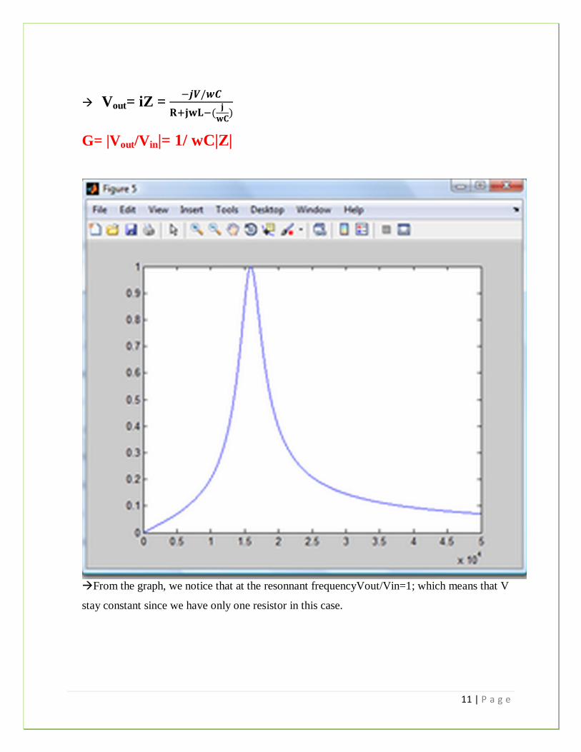
Vout= iZ =

G= |Vout/Vin|= 1/ wC|Z|

From the graph, we notice that at the resonnant frequencyVout/Vin=1; which means that V

stay constant since we have only one resistor in this case.

12 | P a g e

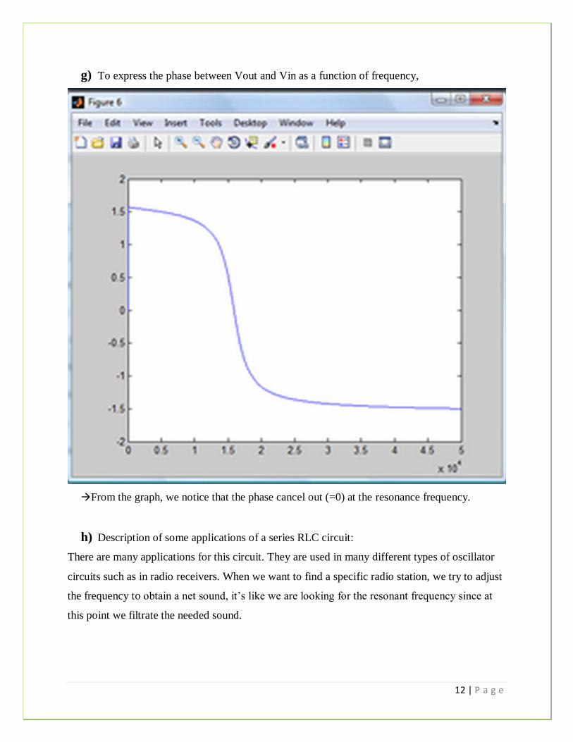
g) To express the phase between Vout and Vin as a function of frequency,

From the graph, we notice that the phase cancel out (=0) at the resonance frequency.

h) Description of some applications of a series RLC circuit:

There are many applications for this circuit. They are used in many different types of oscillator

circuits such as in radio receivers. When we want to find a specific radio station, we try to adjust

the frequency to obtain a net sound, it’s like we are looking for the resonant frequency since at

this point we filtrate the needed sound.

13 | P a g e

B. Simulation:

a) Setting up an AC analysis:

To set up the AC analysis, we followed the steps below:

1- From the PSpice menu, we choose: New Simulation

Profile or Edit Simulation Settings. (If this is a new simulation, enter the name of the profile and

click OK.)

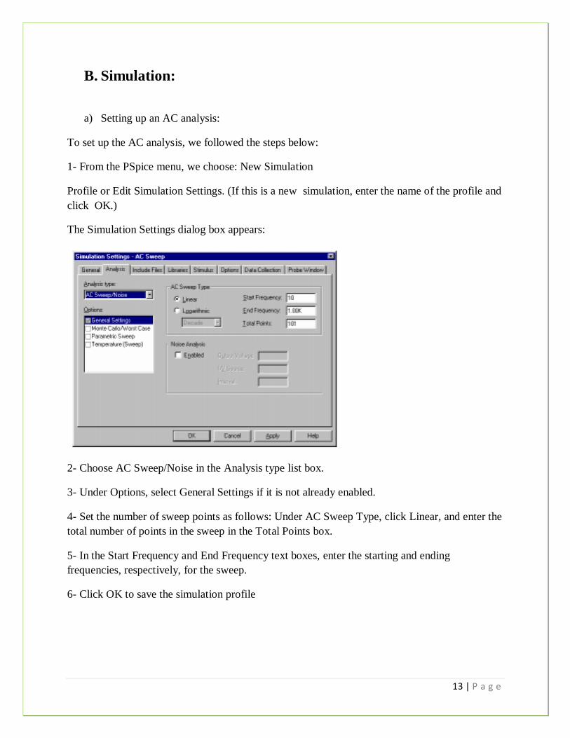
The Simulation Settings dialog box appears:

2- Choose AC Sweep/Noise in the Analysis type list box.

3- Under Options, select General Settings if it is not already enabled.

4- Set the number of sweep points as follows: Under AC Sweep Type, click Linear, and enter the

total number of points in the sweep in the Total Points box.

5- In the Start Frequency and End Frequency text boxes, enter the starting and ending

frequencies, respectively, for the sweep.

6- Click OK to save the simulation profile

14 | P a g e

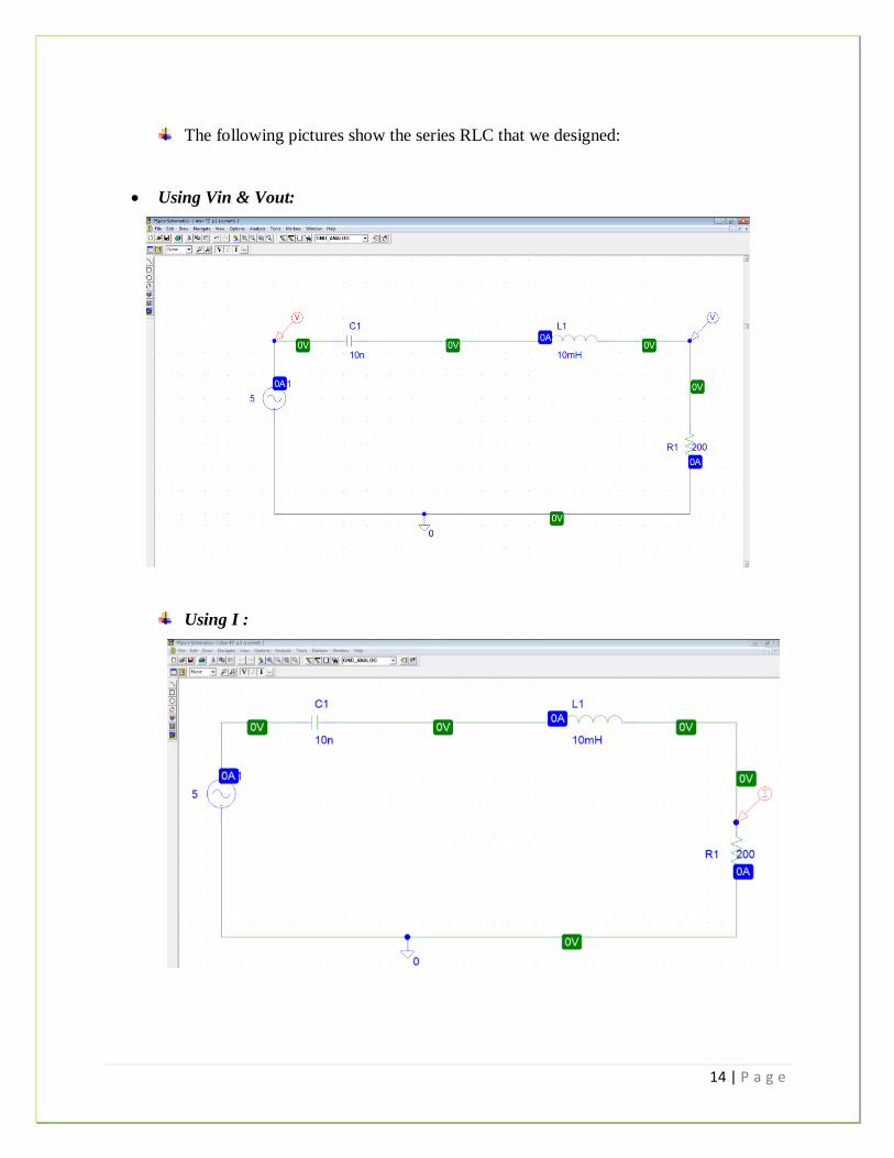
The following pictures show the series RLC that we designed:

Using Vin & Vout:

Using I :

15 | P a g e

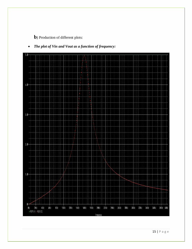
b) Production of different plots:

The plot of Vin and Vout as a function of frequency:

16 | P a g e

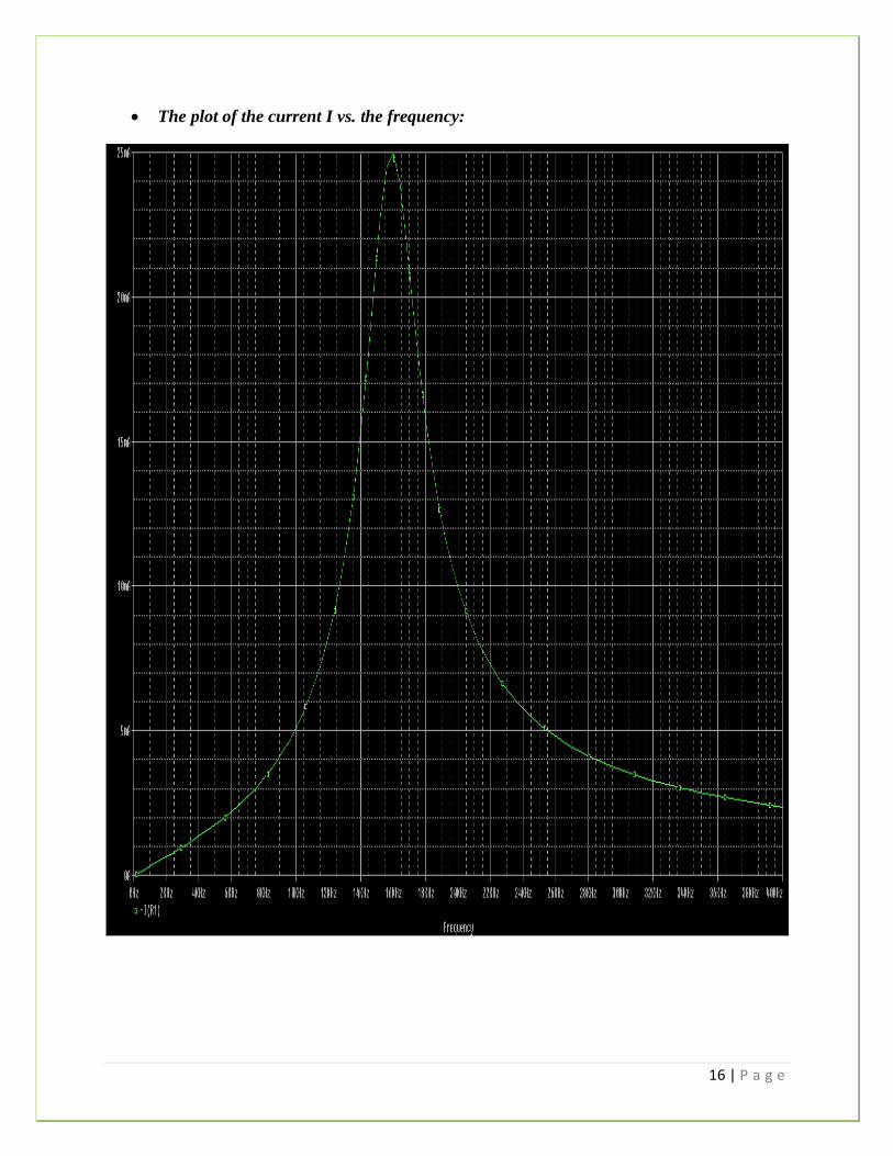
The plot of the current I vs. the frequency:

17 | P a g e

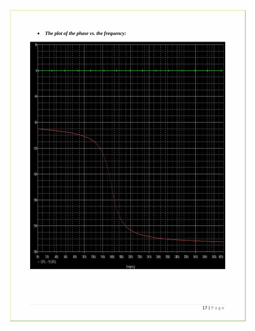
The plot of the phase vs. the frequency:

18 | P a g e

c) From the plots, we deduce that the resonant frequency is the peak of the graph, which

is in our case f= 16 KHz.

From the first graph, Vout/Vin reaches its maximum at the resonant frequency and also we can

notice that the Vout = Vin.

From the second graph, the current reaches its maximum at the resonant frequency.

From the graph 3, the phase cancel out (=0) at the resonant frequency.

Also at the resonant frequency the impedance Z=R which leads that the voltage across the

circuit depends on the resistor R. We have V= I*R= I*Z.

R Z The circuit will perform well its filtrate.

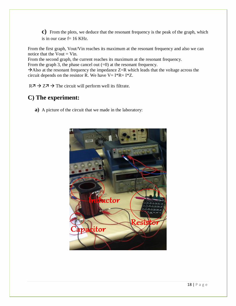
C) The experiment:

a) A picture of the circuit that we made in the laboratory:

19 | P a g e

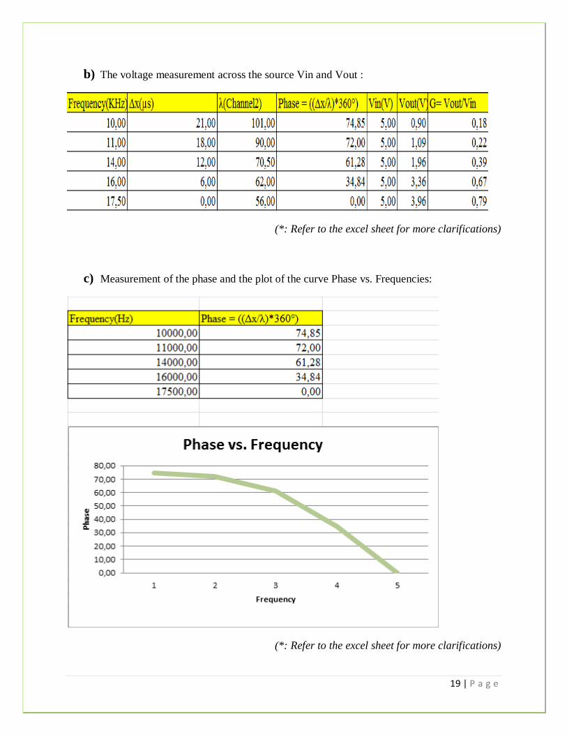
b) The voltage measurement across the source Vin and Vout :

(*: Refer to the excel sheet for more clarifications)

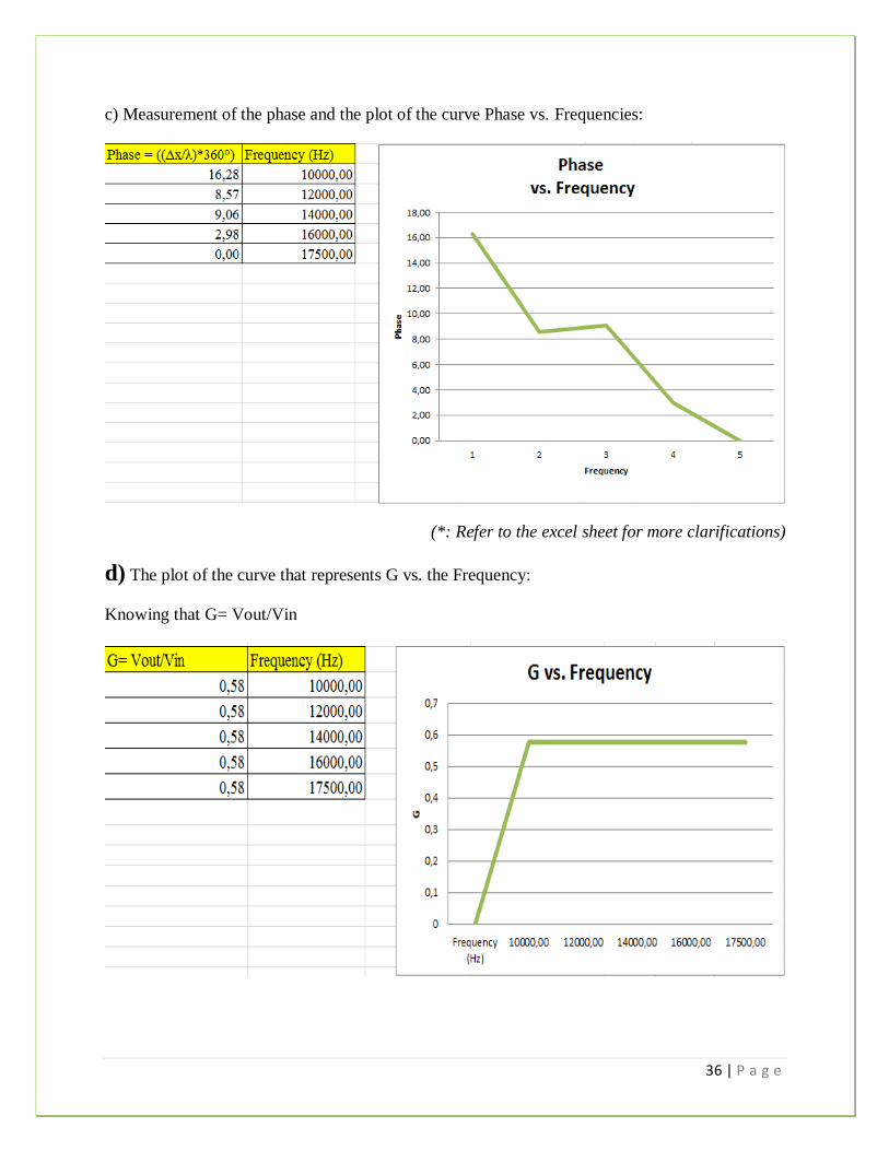
c) Measurement of the phase and the plot of the curve Phase vs. Frequencies:

(*: Refer to the excel sheet for more clarifications)

20 | P a g e

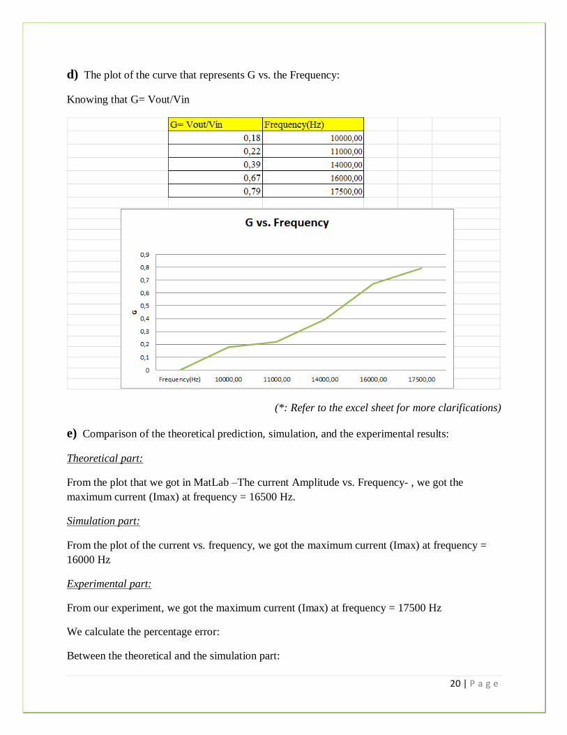
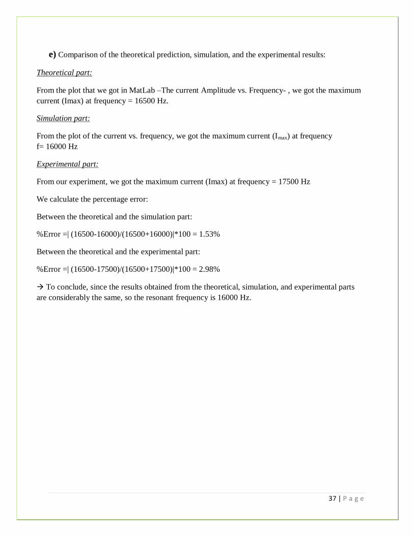
d) The plot of the curve that represents G vs. the Frequency:

Knowing that G= Vout/Vin

(*: Refer to the excel sheet for more clarifications)

e) Comparison of the theoretical prediction, simulation, and the experimental results:

Theoretical part:

From the plot that we got in MatLab –The current Amplitude vs. Frequency- , we got the

maximum current (Imax) at frequency = 16500 Hz.

Simulation part:

From the plot of the current vs. frequency, we got the maximum current (Imax) at frequency =

16000 Hz

Experimental part:

From our experiment, we got the maximum current (Imax) at frequency = 17500 Hz

We calculate the percentage error:

Between the theoretical and the simulation part:

21 | P a g e

%Error =| (16500-16000)/(16500+16000)|*100 = 1.53%

Between the theoretical and the experimental part:

%Error =| (16500-17500)/(16500+17500)|*100 = 2.98%

To conclude, since the results obtained from the theoretical, simulation, and experimental

parts are considerably the same, so the resonant frequency is 16000 Hz.

______________________________________________________________________________

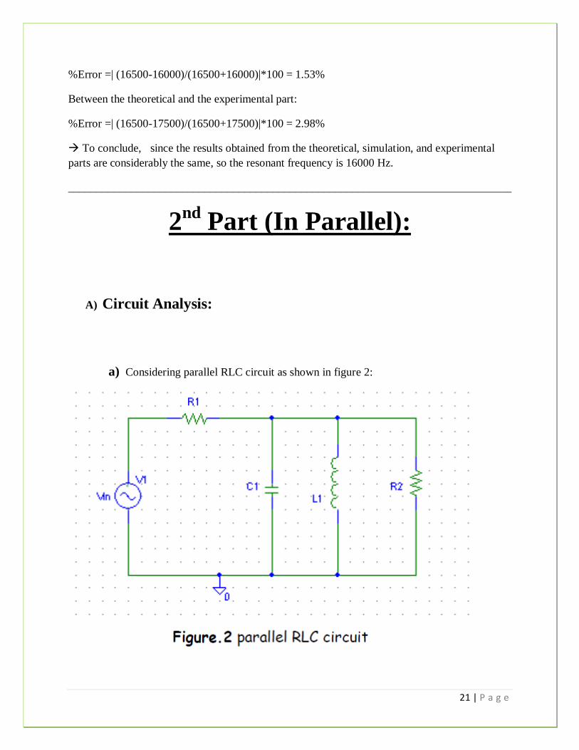
2nd Part (In Parallel):

A) Circuit Analysis:

a) Considering parallel RLC circuit as shown in figure 2:

22 | P a g e

Applying Kirchhoff’s Current Law, we get:

i= iL+iC+iR

di/dt = diL/dt + diC/dt + diR/dt

Knowing that: u= iR *R2 (iR current flowing through R2)

So,

di/dt = ( iR*R2 / L) + (C*R2*d²iR / dt²) + (diR/dt)

b) We solve the differential equation using circuit analysis techniques, we represent the

circuit using the phasors:

ej Ɵ = cos Ɵ + jsin Ɵ

Vin = Vm cos( wt+ Ɵ) = Re{Vme

j (wt+Ɵ) } (Re represents the real part of Vin)

We represent: Vin as Vmej Ɵ

when we work with phasors, the impedances are:

C 1/ jwc = Zc

L jwL = ZL

R ZR

Since ZL ,Zc, ZR are in parallel: Zeq= (jwR2 * L) / (R2+ jwL+w²R2LC)

V = (Vin * Z) / (R1+Z) (V is the voltage across the components)

iR = V/R2 = (Vin*Z) / R2 * (R1+ Z)

Using Kirchhoff’s Law,

-Vin + R1i + Zeqi = 0

So,

i = Vin/ R1+Zeq

23 | P a g e

i depends on R1 and Zeq, when (R1+Zeq) I.

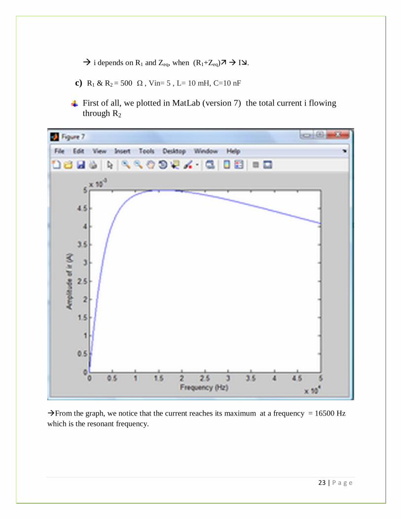
c) R1 & R2 = 500 Ω , Vin= 5 , L= 10 mH, C=10 nF

First of all, we plotted in MatLab (version 7) the total current i flowing

through R2

From the graph, we notice that the current reaches its maximum at a frequency = 16500 Hz

which is the resonant frequency.

24 | P a g e

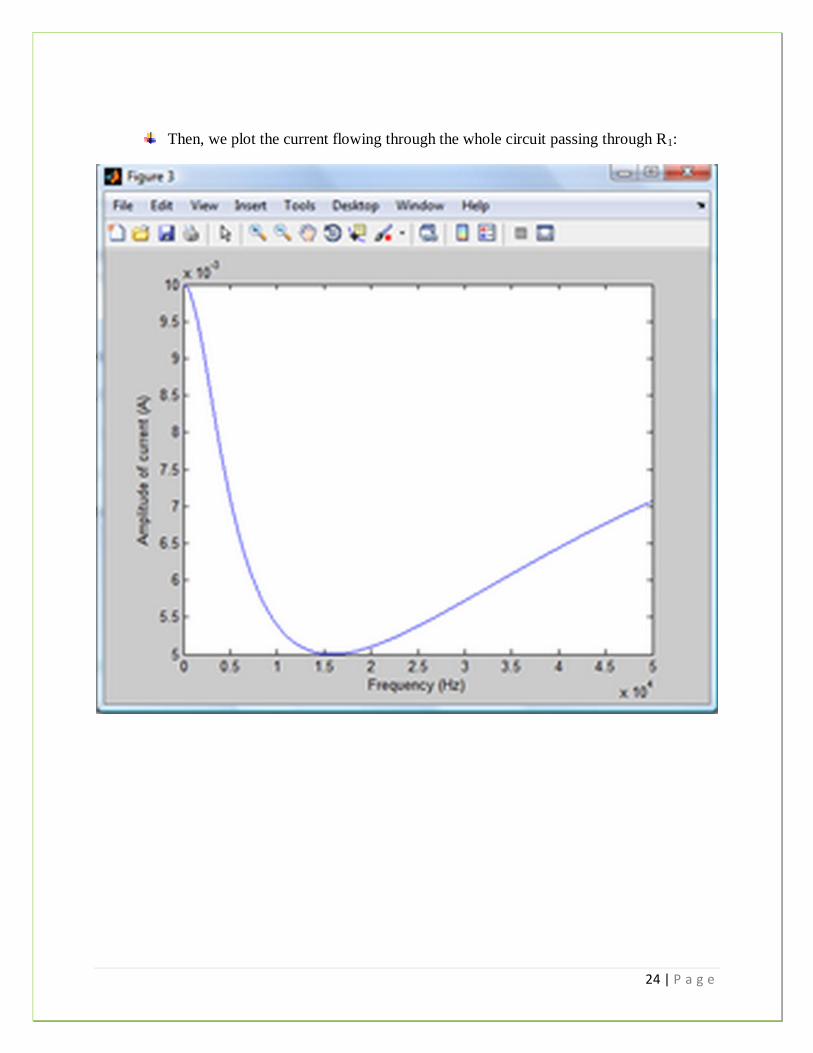
Then, we plot the current flowing through the whole circuit passing through R1:

25 | P a g e

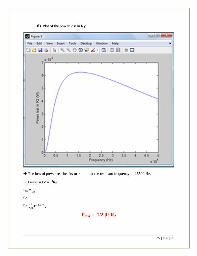
d) Plot of the power lost in R2:

The loss of power reaches its maximum at the resonant frequency f= 16500 Hz.

Power = IV = I2R2

Irms =

So,

P=

* R2

Ploss = 1/2 |I²|R2

26 | P a g e

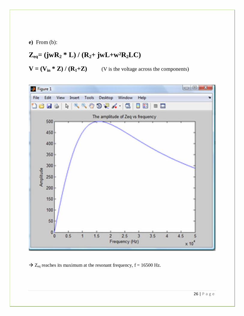
e) From (b):

Zeq= (jwR2 * L) / (R2+ jwL+w²R2LC)

V = (Vin * Z) / (R1+Z) (V is the voltage across the components)

Zeq reaches its maximum at the resonant frequency, f = 16500 Hz.

27 | P a g e

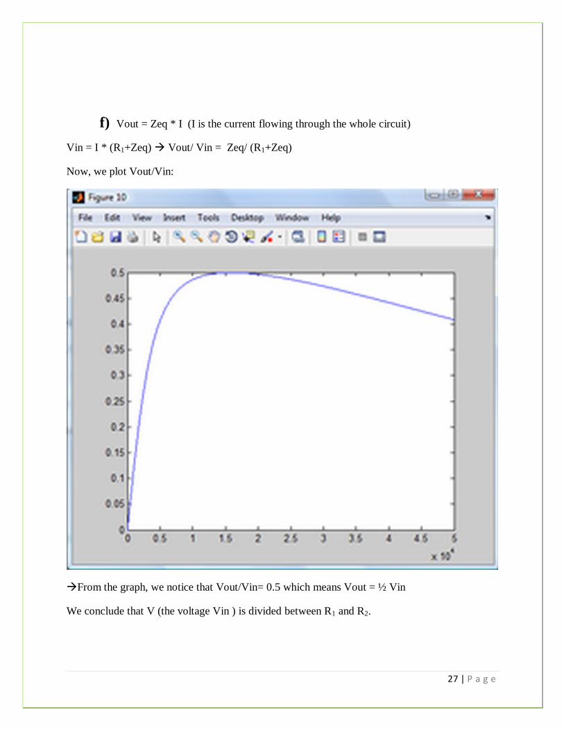
f) Vout = Zeq * I (I is the current flowing through the whole circuit)

Vin = I * (R1+Zeq) Vout/ Vin = Zeq/ (R1+Zeq)

Now, we plot Vout/Vin:

From the graph, we notice that Vout/Vin= 0.5 which means Vout = ½ Vin

We conclude that V (the voltage Vin ) is divided between R1 and R2.

28 | P a g e

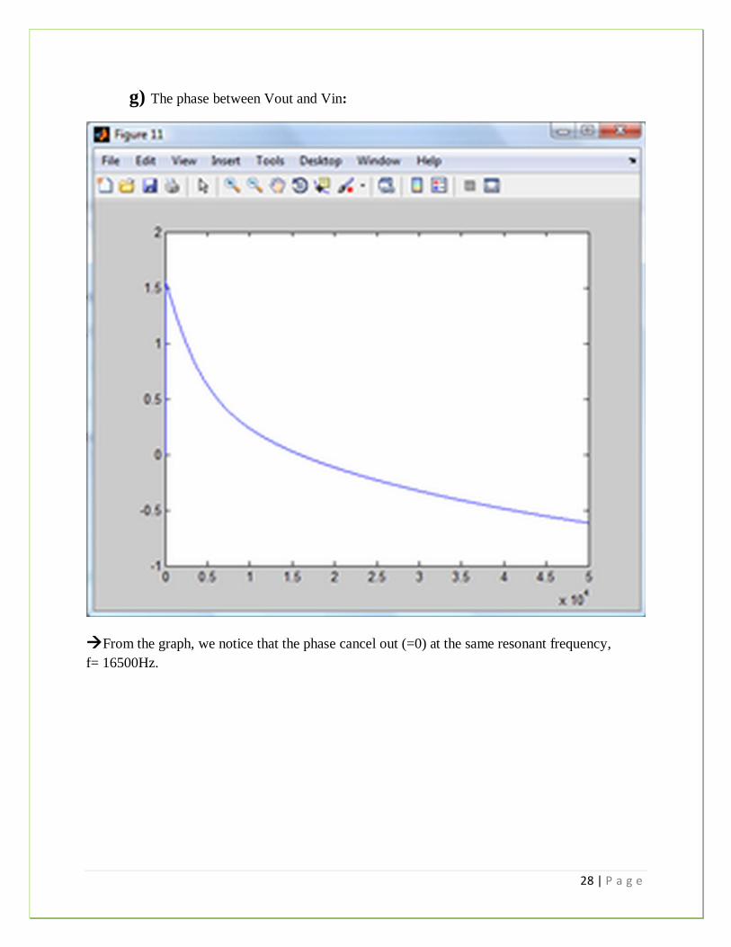
g) The phase between Vout and Vin:

From the graph, we notice that the phase cancel out (=0) at the same resonant frequency,

f= 16500Hz.

29 | P a g e

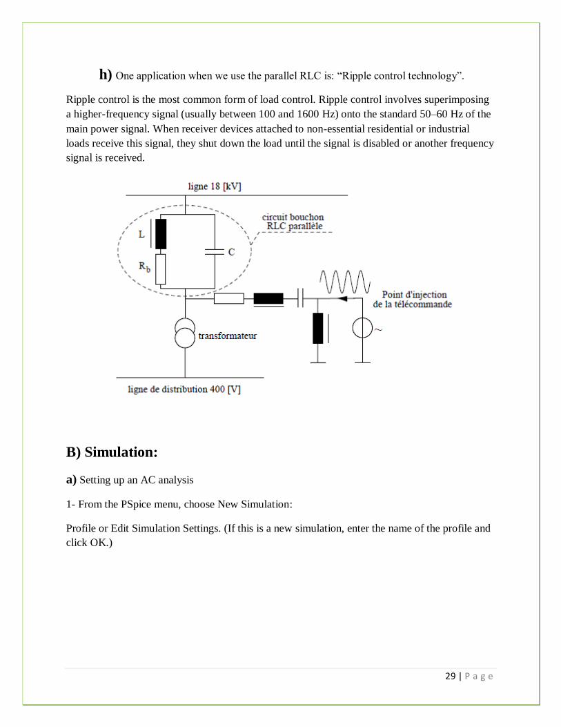
h) One application when we use the parallel RLC is: “Ripple control technology”.

Ripple control is the most common form of load control. Ripple control involves superimposing

a higher-frequency signal (usually between 100 and 1600 Hz) onto the standard 50–60 Hz of the

main power signal. When receiver devices attached to non-essential residential or industrial

loads receive this signal, they shut down the load until the signal is disabled or another frequency

signal is received.

B) Simulation:

a) Setting up an AC analysis

1- From the PSpice menu, choose New Simulation:

Profile or Edit Simulation Settings. (If this is a new simulation, enter the name of the profile and

click OK.)

30 | P a g e

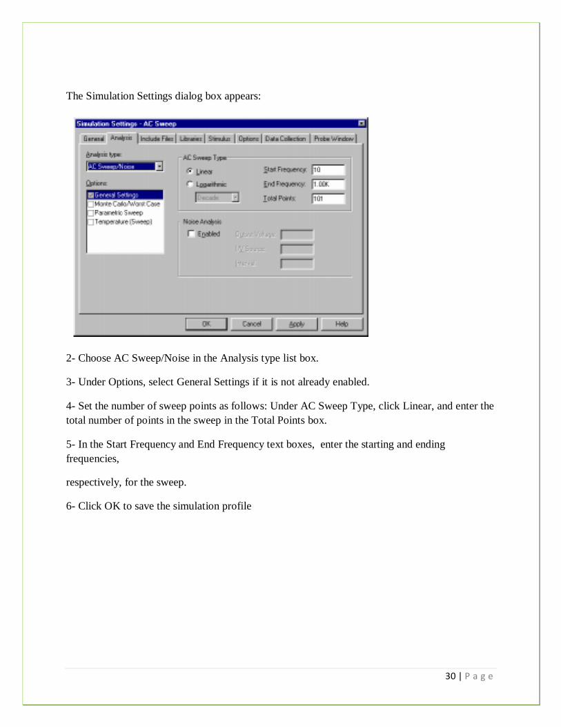
The Simulation Settings dialog box appears:

2- Choose AC Sweep/Noise in the Analysis type list box.

3- Under Options, select General Settings if it is not already enabled.

4- Set the number of sweep points as follows: Under AC Sweep Type, click Linear, and enter the

total number of points in the sweep in the Total Points box.

5- In the Start Frequency and End Frequency text boxes, enter the starting and ending

frequencies,

respectively, for the sweep.

6- Click OK to save the simulation profile

31 | P a g e

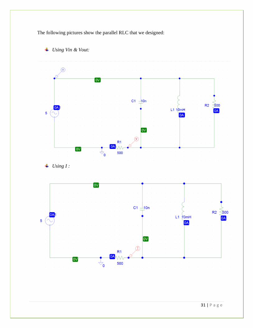
The following pictures show the parallel RLC that we designed:

Using Vin & Vout:

Using I :

32 | P a g e

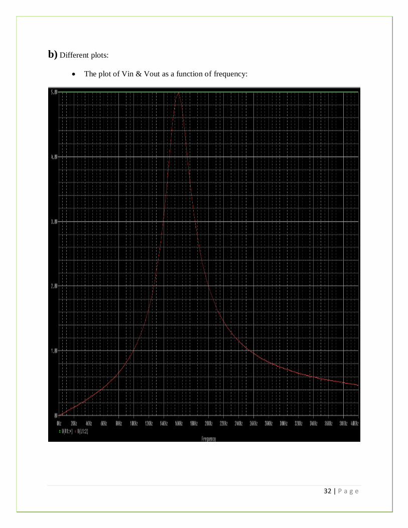
b) Different plots:

The plot of Vin & Vout as a function of frequency:

33 | P a g e

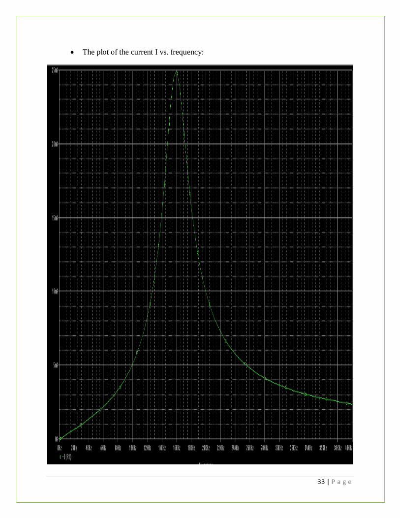
The plot of the current I vs. frequency:

34 | P a g e

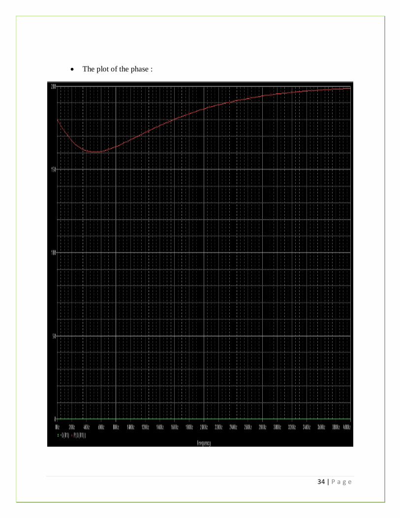
The plot of the phase :

35 | P a g e

c) From the plots, we deduce that the resonant frequency is the peak of the graph, which

is in our case f= 16500 Hz.

From the first graph, Vout/Vin reaches its maximum at the resonant frequency and also we can

notice that the Vout = ½ Vin Vin is divided between R1 and R2.

From the second graph, the current reaches its maximum at the resonant frequency.

From the graph 3, the phase cancel out (=0) at the resonant frequency.

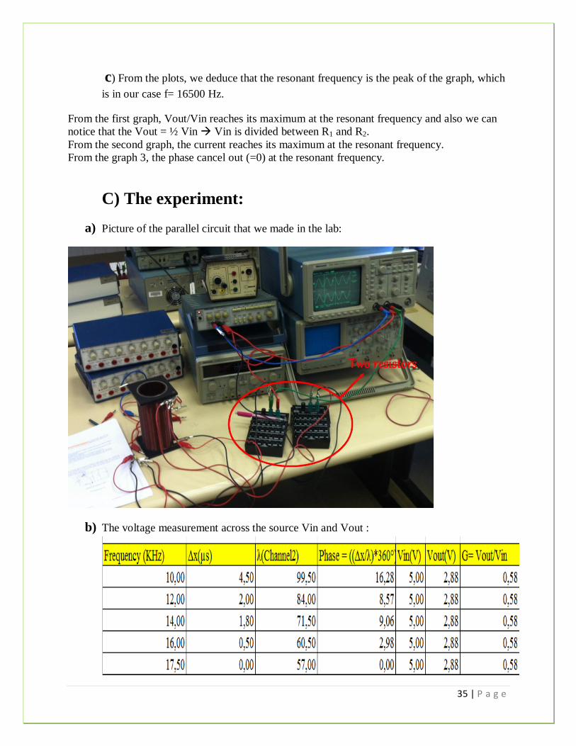
C) The experiment:

a) Picture of the parallel circuit that we made in the lab:

b) The voltage measurement across the source Vin and Vout :

36 | P a g e

c) Measurement of the phase and the plot of the curve Phase vs. Frequencies:

(*: Refer to the excel sheet for more clarifications)

d) The plot of the curve that represents G vs. the Frequency:

Knowing that G= Vout/Vin

37 | P a g e

e) Comparison of the theoretical prediction, simulation, and the experimental results:

Theoretical part:

From the plot that we got in MatLab –The current Amplitude vs. Frequency- , we got the maximum

current (Imax) at frequency = 16500 Hz.

Simulation part:

From the plot of the current vs. frequency, we got the maximum current (Imax) at frequency

f= 16000 Hz

Experimental part:

From our experiment, we got the maximum current (Imax) at frequency = 17500 Hz

We calculate the percentage error:

Between the theoretical and the simulation part:

%Error =| (16500-16000)/(16500+16000)|*100 = 1.53%

Between the theoretical and the experimental part:

%Error =| (16500-17500)/(16500+17500)|*100 = 2.98%

To conclude, since the results obtained from the theoretical, simulation, and experimental parts

are considerably the same, so the resonant frequency is 16000 Hz.

38 | P a g e

Conclusion:

We have seen so far that series and parallel RLC circuits contain both capacitive reactance and

inductive reactance within the same circuit. If we vary the frequency across these circuits there

must become a point where the capacitive reactance value equals that of the inductive reactance

and therefore, XC = XL. The frequency point at which this occurs is called resonance. Also, from

this experiment, we noticed that the range of the frequencies in the parallel RLC circuit is bigger

than the range of the series RLC circuit. This leads us to conclude that the series RLC filter

better than the parallel RLC.