Embed Size (px)
Citation preview

Dept. of Internet & Multimedia Eng., Changhoon YimR.C. Gonzalez & R.E. Woods 1
Chapter 3: Image Enhancement in the Spatial Domain
Chapter 3: Image Enhancement in the Spatial Domain
3.1 Background
3.2 Some basic intensity transformation functions
3.3 Histogram processing
3.4 Fundamentals of spatial filtering
3.5 Smoothing spatial filters
3.6 Sharpening spatial filters

Dept. of Internet & Multimedia Eng., Changhoon YimR.C. Gonzalez & R.E. Woods 2
PreviewPreview
• Spatial domain processing: direct manipulation of pixels in an image
• Two categories of spatial (domain) processing
• Intensity transformation:
- Operate on single pixels
- Contrast manipulation, image thresholding
• Spatial filtering
- Work in a neighborhood of every pixel in an image
- Image smoothing, image sharpening

Dept. of Internet & Multimedia Eng., Changhoon YimR.C. Gonzalez & R.E. Woods 3
3.1 Background3.1 Background
• Spatial domain methods: operate directly on pixels
• Spatial domain processing
g(x,y) = T[f(x, y)]
f(x, y): input image
g(x, y): output (processed) image
T: operator
• Operator T is defined over a neighborhood of point (x, y)

Dept. of Internet & Multimedia Eng., Changhoon YimR.C. Gonzalez & R.E. Woods 4
3.1 Background3.1 Background
• For any location (x,y), output image g(x,y) is equal
to the result of applying T to the neighborhood of
(x,y) in f
• Filter: mask, kernel, template, window
Spatial filtering

Dept. of Internet & Multimedia Eng., Changhoon YimR.C. Gonzalez & R.E. Woods 5
3.1 Background3.1 Background
• The simplest form of T: g depends only on the value of f at (x,
y)
T becomes intensity (gray-level) transformation function
s = T(r)
r: intensity of f(x,y)
s: intensity of g(x,y)
• Point processing: enhancement at any point depends only on
the gray level at that point

Dept. of Internet & Multimedia Eng., Changhoon YimR.C. Gonzalez & R.E. Woods 6
3.1 Background3.1 Background
• (a) Contrast stretching
• Values of r below k are compressed into a narrow range of s
• (b) Thresholding
Point processing

Dept. of Internet & Multimedia Eng., Changhoon YimR.C. Gonzalez & R.E. Woods 7
3.2 Some Basic Intensity Transformation Functions3.2 Some Basic Intensity Transformation Functions
• r: pixel value before processing
s: pixel value after processing
T: transformation
s = T(r)
• 3 types
• Linear (identity and negative transformations)
• Logarithmic (log and inverse-log transformations)
• Power-law (nth power and nth root transformations)

Dept. of Internet & Multimedia Eng., Changhoon YimR.C. Gonzalez & R.E. Woods 8
3.2 Some Basic Gray Level Transformations3.2 Some Basic Gray Level Transformations

Dept. of Internet & Multimedia Eng., Changhoon YimR.C. Gonzalez & R.E. Woods 9
3.2.1 Image Negatives
• Negative of an image with gray level [0, L-1]
s = L – 1 – r
• Enhancing white or gray detail embedded in dark
regions of an image

Dept. of Internet & Multimedia Eng., Changhoon YimR.C. Gonzalez & R.E. Woods 10
3.2.2 Log Transformations
• General form of log transformation
s = c log(1+r)
c: constant, r ≥ 0
• This transformation maps a narrow range of low gray-
level values in the input image into a wider range of
output levels
• Classical application of log transformation:
Display of Fourier spectrum

Dept. of Internet & Multimedia Eng., Changhoon YimR.C. Gonzalez & R.E. Woods 11
3.2.2 Log Transformations
• (a) Original Fourier spectrum: 0 ~ 1,500,000 range
scaled to 0 ~ 255
• (b) Result of log transformation: 0 ~ 6.2 range
scaled to 0 ~ 255

Dept. of Internet & Multimedia Eng., Changhoon YimR.C. Gonzalez & R.E. Woods 12
3.2.3 Power-Law Transformations

Dept. of Internet & Multimedia Eng., Changhoon YimR.C. Gonzalez & R.E. Woods 13
3.2.3 Power-Law Transformations
• Basic form of power-law transformations
s = c r γ
c, γ : positive constants
• Gamma correction:
process of correcting this power-law response
• Example: cathode ray tube (CRT)
Intensity to voltage response is power function with
exponent (γ) 1.8 to 2.5
Solution: preprocess the input image by performing
transformation
s = r1/2.5 = r0.4

Dept. of Internet & Multimedia Eng., Changhoon YimR.C. Gonzalez & R.E. Woods 14
3.2.3 Power-Law Transformations
CRT monitor gamma correction
example

Dept. of Internet & Multimedia Eng., Changhoon YimR.C. Gonzalez & R.E. Woods 15
3.2.3 Power-Law Transformations
MRI gamma correction example
original γ = 0.6
γ = 0.4 γ = 0.3

Dept. of Internet & Multimedia Eng., Changhoon YimR.C. Gonzalez & R.E. Woods 16
3.2.3 Power-Law Transformations
Arial image gamma correction
example
originalγ =
3.0
γ =
5.0
γ =
4.0

Dept. of Internet & Multimedia Eng., Changhoon YimR.C. Gonzalez & R.E. Woods 17
3.2.4 Piecewise-Linear Transformation Functions
Contrast stretching
Piecewise
linear
function
Low contrast
image
Result of
contrast
stretching
Result of
thresholding

Dept. of Internet & Multimedia Eng., Changhoon YimR.C. Gonzalez & R.E. Woods 18
3.2.4 Piecewise-Linear Transformation Functions
Contrast
stretching(c) Contrast stretching
(r1, s1) = (rmin, 0), (r2, s2) = (rmax, L-1)
rmin, rmax: minimum, maxmum level of image
(d) Thresholding:
r1 = r2 = m, s1 = 0, s2 = L-1
m: mean gray level

Dept. of Internet & Multimedia Eng., Changhoon YimR.C. Gonzalez & R.E. Woods 19
3.2.4 Piecewise-Linear Transformation Functions
Intensity-level slicing

Dept. of Internet & Multimedia Eng., Changhoon YimR.C. Gonzalez & R.E. Woods 20
3.2.4 Piecewise-Linear Transformation Functions
Intensity-level slicing
(a) Display a high value for all gray levels in the
range of interest, and a low value for all other
images
- produces binary image
(b) Brightens the desired range of gray levels
but preserves the background and other parts

Dept. of Internet & Multimedia Eng., Changhoon YimR.C. Gonzalez & R.E. Woods 21
3.2.4 Piecewise-Linear Transformation Functions
Intensity-level slicing

Dept. of Internet & Multimedia Eng., Changhoon YimR.C. Gonzalez & R.E. Woods 22
3.2.4 Piecewise-Linear Transformation Functions
Bit-plane
slicing

Dept. of Internet & Multimedia Eng., Changhoon YimR.C. Gonzalez & R.E. Woods 23
3.2.4 Piecewise-Linear Transformation Functions
Bit-plane
slicing

Dept. of Internet & Multimedia Eng., Changhoon YimR.C. Gonzalez & R.E. Woods 24
3.2.4 Piecewise-Linear Transformation Functions
Bit-plane slicing
(a) Multiply bit plane 8 by 128
Multiply bit plane 7 by 64
Add the results of two planes

Dept. of Internet & Multimedia Eng., Changhoon YimR.C. Gonzalez & R.E. Woods 25
3.3 Histogram Processing3.3 Histogram Processing
• The histogram of digital image with gray levels in the
range [0, L-1] is a discrete function
• h(rk) = nk
rk: kth gray level
nk: number of pixels in image having gray levels rk
• Normalized histogram
p(rk) = nk/n
n: total number of pixels in image
n = MN (M: row dimension, N: column dimension)

Dept. of Internet & Multimedia Eng., Changhoon YimR.C. Gonzalez & R.E. Woods 26
3.3 Histogram Processing3.3 Histogram Processing
Histogram
• horizonal axis:
rk (kth intensity value)
• vertical axis:
nk: number of pixels, or
nk/n: normalized number

Dept. of Internet & Multimedia Eng., Changhoon YimR.C. Gonzalez & R.E. Woods 27
3.3.1 Histogram Equalization
• r: intensities of the image to be enhanced
r is in the range [0, L-1]
r = 0: black, r = L-1: white
s: processed gray levels for every pixel value r
• s = T(r), 0 ≤ r ≤ L-1
• Requirements of transformation function T
(a) T(r) is a (strictly) monotonically increasing in the
interval 0 ≤ r ≤ L-1
(b) 0 ≤ T(r) ≤ L-1 for 0 ≤ r ≤ L-1 • Inverse transformation
r = T-1(s), 0 ≤s ≤L-1

Dept. of Internet & Multimedia Eng., Changhoon YimR.C. Gonzalez & R.E. Woods 28
3.3.1 Histogram Equalization
Intensity transformation function

Dept. of Internet & Multimedia Eng., Changhoon YimR.C. Gonzalez & R.E. Woods 29
3.3.1 Histogram Equalization
( ) ( )s r
drp s p r
ds
0( ) ( 1) ( )
r
rs T r L p w dw
0
( )( 1) [ ( ) ] ( 1) ( )
r
r r
ds dT r dL p w dw L p r
dr dr dr
1 1( ) ( ) ( )
( 1) ( ) 1s r rr
drp s p r p r
ds L p r L
probability density function (PDF)
cumulative distribution function (CDF)
Uniform probability density function
Intensity levels: random variable in interval [0, L-1]
0 1s L

Dept. of Internet & Multimedia Eng., Changhoon YimR.C. Gonzalez & R.E. Woods 30
3.3.1 Histogram Equalization

Dept. of Internet & Multimedia Eng., Changhoon YimR.C. Gonzalez & R.E. Woods 31
3.3.1 Histogram Equalization
( ) 0,1,2,..., 1kr k
np r k L
MN
0 0
1( ) ( 1) ( ) 0,1,2,.., 1
k k
k k r j jj j
Ls T r L p r n k L
MN
• histogram equalization (histogram linearization):
Processed image is obtained by mapping each pixel rk (input
image)
into corresponding level sk (output image)
MN: total number of pixels in image
nk: number of pixels having gray level rk
L: total number of possible gray levels

Dept. of Internet & Multimedia Eng., Changhoon YimR.C. Gonzalez & R.E. Woods 32
3.3.1 Histogram Equalization

Dept. of Internet & Multimedia Eng., Changhoon YimR.C. Gonzalez & R.E. Woods 33
3.3.1 Histogram Equalization
Histogram equalization from dark image (1)
Histogram equalization from light image (2)
Histogram equalization from low contrast image (3)
Histogram equalization from high contrast image (4)

Dept. of Internet & Multimedia Eng., Changhoon YimR.C. Gonzalez & R.E. Woods 34
3.3.1 Histogram Equalization
Transformation functions

Dept. of Internet & Multimedia Eng., Changhoon YimR.C. Gonzalez & R.E. Woods 35
3.3.3 Local Histogram Processing
• Histogram processing methods in previous section are
global
• Global methods are suitable for overall enhancement
• Histogram processing techniques are easily adapted to
local enhancement
• Example
(b) Global histogram equalization
Considerable enhancement of noise
(c) Local histogram equalization using 7x7 neighborhood
Reveals (enhances) the small squares inside the dark
squares
Contains finer noise texture

Dept. of Internet & Multimedia Eng., Changhoon YimR.C. Gonzalez & R.E. Woods 36
3.3.3 Local Histogram Processing
Original imageGlobal histogramequalized image
Local histogramequalized image

Dept. of Internet & Multimedia Eng., Changhoon YimR.C. Gonzalez & R.E. Woods 37
3.3.4 Use of Histogram Statistics for Image Enhancement
1
0
( ) ( ) ( )L
nn i i
i
r r m p r
1
0
( )L
i ii
m r p r
12
20
( ) ( ) ( )L
i ii
r r m p r
r: discrete random variable representing intensity values in the range [0, L-1]
p(ri): normalized histogram component corresponding to value ri
nth moment of r
mean (average) value of r
variance of r, б2(r)
1 1
0 0
1( , )
M N
x y
m f x yMN
sample mean
1 12 2
0 0
1[ ( , ) ]
M N
x y
f x y mMN
sample variance

Dept. of Internet & Multimedia Eng., Changhoon YimR.C. Gonzalez & R.E. Woods 38
3.3.4 Use of Histogram Statistics for Image Enhancement
1
0
( )xy xy
L
S i S ii
m r p r
12 2
0
( ) ( )xy xy xy
L
S i S S ii
r m p r
• Global mean and variance are measured over entire image
Used for gross adjustment of overall intensity and contrast
• Local mean and variance are measured locally
Used for local adjustment of local intensity and contrast
local mean
local variance
(x,y): coordinate of a pixel
Sxy: neighborhood (subimage), centered on (x,y)
r0, …, rL-1: L possible intensity values
pSxy: histogram of pixels in region Sxy

Dept. of Internet & Multimedia Eng., Changhoon YimR.C. Gonzalez & R.E. Woods 39
3.3.4 Use of Histogram Statistics for Image Enhancement
• A measure whether an area is relatively light or dark at (x,y) Compare the local average gray level mSxy to the global mean mG
(x,y) is a candidate for enhancement if mSxy ≤ k0mG
• Enhance areas that have low contrast Compare the local standard deviation бSxy to the global standard deviation бG
(x,y) is a candidate for enhancement if бSxy ≤ k2 бG
• Restrict lowest values of contrast (x,y) is a candidate for enhancement if k1 бG ≤ бSxy • Enhancement is processed simply multiplying the gray level by a constant E 0 1 2( , ) if
( , )( , ) otherwise
xy xyS G G S GE f x y m k m AND k kg x y
f x y

Dept. of Internet & Multimedia Eng., Changhoon YimR.C. Gonzalez & R.E. Woods 40
3.3.4 Use of Histogram Statistics for Image Enhancement
Problem: enhance dark areas while leaving the light area as unchanged as possible
E = 4.0, k0 = 0.4, k1 = 0.02, k2 = 0.4, Local region (neighborhood) size: 3x3

Dept. of Internet & Multimedia Eng., Changhoon YimChap.3 Intensity Transformations and Spatial Filtering 41
3.4 Fundamentals of Spatial Filtering3.4 Fundamentals of Spatial Filtering
• Operations with the values of the image pixels in the neighborhood
and the corresponding values of subimage
• Subimage: filter, mask, kernel, template, window
• Values in the filter subimage: coefficient
• Spatial filtering operations are performed directly on the pixels
of an image
• One-to-one correspondence between
linear spatial filters and filters in the frequency domain

Dept. of Internet & Multimedia Eng., Changhoon YimChap.3 Intensity Transformations and Spatial Filtering 42
• A spatial filter consists of
(1) a neighborhood (typically a small rectangle)
(2) a predefined operation
• A processed (filtered) image is generated as the center of
the filter visits each pixel in the input image
• Linear spatial filtering using 3x3 neighborhood
• At any point (x,y), the response, g(x,y), of the filter
g(x,y) = w(-1,-1)f(x-1,y-1) + w(-1,0)f(x-1,y) + …
+ w(0,0)f(x,y) + …+ w(1,0)f(x+1,y) + w(1,1)f(x+1,y+1)
3.4.1 Mechanics of Spatial Filtering

Dept. of Internet & Multimedia Eng., Changhoon YimChap.3 Intensity Transformations and Spatial Filtering 43
3.4.1 Mechanics of Spatial Filtering

Dept. of Internet & Multimedia Eng., Changhoon YimChap.3 Intensity Transformations and Spatial Filtering 44
( , ) ( , ) ( , )a b
s a t b
g x y w s t f x s y t
• Filtering of an image f with a filter w of size m x n
a = (m-1) / 2, b = (n-1) / 2 or m = 2a+1, n = 2b+1
(a, b: positive integer)
3.4.1 Mechanics of Spatial Filtering

Dept. of Internet & Multimedia Eng., Changhoon YimChap.3 Intensity Transformations and Spatial Filtering 45
3.4.2 Spatial Correlation and Convolution

Dept. of Internet & Multimedia Eng., Changhoon YimChap.3 Intensity Transformations and Spatial Filtering 46
3.4.2 Spatial Correlation and Convolution

Dept. of Internet & Multimedia Eng., Changhoon YimChap.3 Intensity Transformations and Spatial Filtering 47
( , ) ( , ) ( , )a b
s a t b
g x y w s t f x s y t
• Correlation of a filter w(x,y) of size m x n with an image f(x,y)
• Convolution of w(x,y) and f(x,y)
( , ) ( , ) ( , )a b
s a t b
g x y w s t f x s y t
3.4.2 Spatial Correlation and Convolution

Dept. of Internet & Multimedia Eng., Changhoon YimChap.3 Intensity Transformations and Spatial Filtering 48
1 1 2 21
mnT
mn mn i ii
R w z w z w z w z
w z
• Linear spatial filtering by m x n filter
• Linear spatial filtering by 3 x 3 filter
9
1 1 2 2 9 91
Ti i
i
R w z w z w z w z
w z
3.4.3 Vector Representation of Linear Filtering

Dept. of Internet & Multimedia Eng., Changhoon YimChap.3 Intensity Transformations and Spatial Filtering 49
• Spatial filtering at the border of an image• Limit the center of the mask no less than (n-1)/2 pixels
from the border -> Smaller filtered image• Padding -> Effect near the border
• Adding rows and columns of 0’s• Replicating rows and columns
3.4.3 Vector Representation of Linear Filtering

Dept. of Internet & Multimedia Eng., Changhoon YimChap.3 Intensity Transformations and Spatial Filtering 50
• Linear spatial filtering by 3 x 3 filter
9
1 1 2 2 9 91
i ii
R w z w z w z w z
3.4.4 Generating Spatial Filter Masks
• Average value in 3 x 3 neighborhood
9
1
1
9 ii
R z
• Gaussian function
2 2
22( , )x y
h x y e

Dept. of Internet & Multimedia Eng., Changhoon YimChap.3 Intensity Transformations and Spatial Filtering 51
3.5 Smoothing Spatial Filters3.5 Smoothing Spatial Filters
• Linear spatial filters for smoothing:
averaging filters, lowpass filters• Noise reduction• Undesirable side effect: blur
edges
standard average
weighted average

Dept. of Internet & Multimedia Eng., Changhoon YimChap.3 Intensity Transformations and Spatial Filtering 52
• Standard averaging by 3x3 filter 9
1
1
9 ii
R z
• Weighted averaging
Reduce blurring compared to standard
averaging
( , ) ( , )( , )
( , )
a b
s a t ba b
s a t b
w s t f x s y tg x y
w s t
• General implementation for filtering with a
weighted
averaging filter of size m x n (m=2a+1, n=2b+1)
3.5.1 Smoothing Linear Filters

Dept. of Internet & Multimedia Eng., Changhoon YimChap.3 Intensity Transformations and Spatial Filtering 53
3.5.1 Smoothing Linear Filters
Result of smoothing with square averaging filter masks
Original n=3
n=5 n=9
n=15 n=35

Dept. of Internet & Multimedia Eng., Changhoon YimChap.3 Intensity Transformations and Spatial Filtering 54
3.5.1 Smoothing Linear Filters
Application example of spatial averaging
15x15 averaging Result of thresholdingOriginal

Dept. of Internet & Multimedia Eng., Changhoon YimChap.3 Intensity Transformations and Spatial Filtering 55
3.5.2 Order-Statistic (Nonlinear) Filters
• Order-statistic filters are nonlinear spatial filters whose response is based on ordering (ranking) the pixels• Median filter• Replaces the pixel value by the median of the gray levels
in the neighborhood of that pixel• Effective for impulse noise (salt-and-pepper noise)• Isolated clusters of pixels that are light or dark
with respect to their neighbors, and whose area is less than n2/2, are eliminated by an n x n median filter• Median
• 3x3 neighborhood: 5th largest value• 5x5 neighborhood: 13th largest value
• Max filter: select maximum value in the neighborhood• Min filter: select minimum value in the neighborhood

Dept. of Internet & Multimedia Eng., Changhoon YimChap.3 Intensity Transformations and Spatial Filtering 56
3.5.2 Order-Statistic Filters

Dept. of Internet & Multimedia Eng., Changhoon YimChap.3 Intensity Transformations and Spatial Filtering 57
3.6 Sharpening Spatial Filters3.6 Sharpening Spatial Filters
• Objective of sharpening:
highlight fine detail to enhance detail that has been blurred
• Image blurring can be accomplished by digital averaging
Digital averaging is similar to spatial integration
• Image sharpening can be done by digital differentiation
Digital differentiation is similar to spatial derivative
• Image differentiation enhances edges and other discontinuities
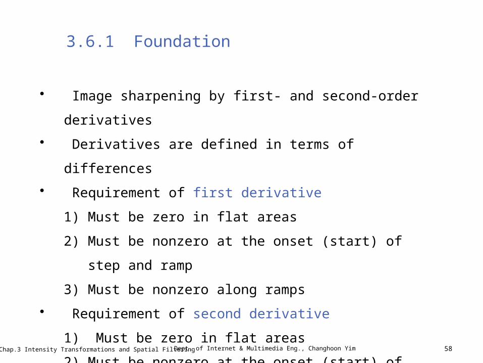
Dept. of Internet & Multimedia Eng., Changhoon YimChap.3 Intensity Transformations and Spatial Filtering 58
• Image sharpening by first- and second-order
derivatives
• Derivatives are defined in terms of differences
• Requirement of first derivative
1) Must be zero in flat areas
2) Must be nonzero at the onset (start) of step and
ramp
3) Must be nonzero along ramps
• Requirement of second derivative
1) Must be zero in flat areas
2) Must be nonzero at the onset (start) of step and
ramp
3) Must be zero along ramps of constant slope
3.6.1 Foundation

Dept. of Internet & Multimedia Eng., Changhoon YimChap.3 Intensity Transformations and Spatial Filtering 59
3.6.1 Foundation
( ) ( 1) ( )fx f x f x
x
2
2( 1) ( 1) 2 ( )
ff x f x f x
x
first-order derivative
second-order derivative
( 1) ( ) ( 1)fx f x f x
x

Dept. of Internet & Multimedia Eng., Changhoon YimChap.3 Intensity Transformations and Spatial Filtering 60
3.6.1 Foundation

Dept. of Internet & Multimedia Eng., Changhoon YimChap.3 Intensity Transformations and Spatial Filtering 61
3.6.1 Foundation
• At the ramp• First-order derivative is nonzero along the ramp • Second-order derivative is zero along the ramp• Second-order derivative is nonzero only at the onset and end
of the ramp• At the step
• Both the first- and second-order derivatives are nonzero• Second-order derivative has a transition from positive to negative
(zero crossing)• Some conclusions
• First-order derivatives generally produce thicker edges• Second-order derivatives have stronger response to fine detail• First-order derivatives generally produce stronger response
to gray-level step• Second-order derivatives produce a double response at step

Dept. of Internet & Multimedia Eng., Changhoon YimChap.3 Intensity Transformations and Spatial Filtering 62
3.6.2 Use of Second Derivatives for Enhancement
• Isotropic filters: rotation invariant
• Simplest isotropic second-order derivative operator: Laplacian
2 22
2 2
f ff
x y
2-D Laplacian operation
2
2( 1, ) ( 1, ) 2 ( , )
ff x y f x y f x y
x
2
2( , 1) ( , 1) 2 ( , )
ff x y f x y f x y
y
2 ( , ) [ ( 1, ) ( 1, ) ( , 1) ( , 1)] 4 ( , )f x y f x y f x y f x y f x y f x y
x-direction
y-direction

Dept. of Internet & Multimedia Eng., Changhoon YimChap.3 Intensity Transformations and Spatial Filtering 63
3.6.2 Use of Second Derivatives for Enhancement
4 neighborsnegative center coefficient
8 neighborsnegative center coefficient
4 neighborspositive center coefficient
8 neighborspositive center coefficient

Dept. of Internet & Multimedia Eng., Changhoon YimChap.3 Intensity Transformations and Spatial Filtering 64
3.6.2 Use of Second Derivatives for Enhancement
• Image enhancement (sharpening) by Laplacian operation
2
2
( , ) ( , ) if the center coefficient of the Laplacian mask is negative( , )
( , ) ( , ) if the center coefficient of the Laplacian mask is positive
f x y f x y
g x yf x y f x y
( , ) ( , ) [ ( 1, ) ( 1, ) ( , 1)( , 1)] 4 ( , )
5 ( , ) [ ( 1, ) ( 1, )( , 1) ( , 1)]
g x y f x y f x y f x y f x yf x y f x yf x y f x y f x yf x y f x y
• Simplification

Dept. of Internet & Multimedia Eng., Changhoon YimChap.3 Intensity Transformations and Spatial Filtering 65
3.6.2 Use of Second Derivatives for Enhancement
Original image
Laplacian image
Enhanced image(original-Laplacian)

Dept. of Internet & Multimedia Eng., Changhoon YimChap.3 Intensity Transformations and Spatial Filtering 66
3.6.2 Use of Second Derivatives for Enhancement
Original image
Enhanced image8 neighbors
Enhanced image4 neighbors

Dept. of Internet & Multimedia Eng., Changhoon YimChap.3 Intensity Transformations and Spatial Filtering 67
3.6.3 Unsharp Masking and Highboost Filtering
( , ) ( , ) ( , )maskg x y f x y f x y
• When k=1, unsharp masking
• When k > 1, highboost filtering
original image – blurred image
( , ) ( , ) ( , )maskg x y f x y k g x y

Dept. of Internet & Multimedia Eng., Changhoon YimChap.3 Intensity Transformations and Spatial Filtering 68
3.6.3 Unsharp Masking and Highboost Filtering

Dept. of Internet & Multimedia Eng., Changhoon YimChap.3 Intensity Transformations and Spatial Filtering 69
3.6.3 Unsharp Masking and Highboost Filtering

Dept. of Internet & Multimedia Eng., Changhoon YimChap.3 Intensity Transformations and Spatial Filtering 70
3.6.4 Using First-Order Derivatives for Image Sharpening
grad( )f
x xf
y y
gf f g
2 2 1/ 2
1/ 222
( , ) mag( ) [ ]x yM x y f g g
f f
x y
• First derivatives in image processing is implemented
using the magnitude of the gradient
gradient of f at (x,y)
magnitude of gradient
( , ) x yM x y g g Approximation of magnitude of gradient by absolute values

Dept. of Internet & Multimedia Eng., Changhoon YimChap.3 Intensity Transformations and Spatial Filtering 71
3x3 region
Roberts operators
Sobel operators
3.6.4 Using First-Order Derivatives for Image Sharpening

Dept. of Internet & Multimedia Eng., Changhoon YimChap.3 Intensity Transformations and Spatial Filtering 72
• Roberts cross-gradient operators
9 5 8 6( ) and ( ) x yg z z g z z
9 5 8 6( , ) x yM x y g g z z z z
3.6.4 Using First-Order Derivatives for Image Sharpening
• Simplest approximation to first-order derivative
8 5 6 5( ) and ( ) x yg z z g z z
2 2 1/ 2 2 2 1/ 29 5 8 6( , ) [ ] [( ) ( ) ]x yM x y g g z z z z

Dept. of Internet & Multimedia Eng., Changhoon YimChap.3 Intensity Transformations and Spatial Filtering 73
• Sobel operators
7 8 9 1 2 3
3 6 9 1 4 7
( 2 ) ( 2 ) and ( 2 ) ( 2 )
x
y
g z z z z z zg z z z z z z
7 8 9 1 2 3
3 6 9 1 4 7
( , )
( 2 ) ( 2 )+ ( 2 ) ( 2 )
x yM x y g g
z z z z z zz z z z z z
3.6.4 Using First-Order Derivatives for Image Sharpening

Dept. of Internet & Multimedia Eng., Changhoon YimChap.3 Intensity Transformations and Spatial Filtering 74
3.7.3 Use of First Derivatives for Enhancement
Optical image of contact lens
Sobel gradient


![rss~'Dce- a.,]) R.e-1ssu1](https://img.pdfslide.us/doc/110x75/5f8f63b590e69168e30c6c5c/rssdce-a-re-1ssu1.jpg)