Embed Size (px)
Citation preview

DEPARTMENT OF ECONOMICS
Working Paper
UNIVERSITY OF MASSACHUSETTS AMHERST
Self-Employed Tutor Pricing Model
by
Tyler Hansen Jared Rand
Working Paper 2016-11

Running head: TUTOR PRICING MODEL 1
Abstract
One of the biggest problems faced by freelance tutors is choosing a price. Too high or too low, and
tutors lose out on earnings. What should a tutor take into account when setting a price? This project
surveys the relevant economic literature—most importantly wage determination—to specify a tutor
pricing model, and then applies econometric methods to test the model. The data set used is from
Knowledge Roundtable, which is a website matching independent tutors to students, and contains data
on 1,250 tutors from around the United States. Using the natural logarithm of tutor price as the
dependent variable, it was found that education level, years of experience (tenure and age), having a
professional certification related to teaching, teaching technical subjects, income level by zip code, and
population density have positive and statistically significant effects on tutor price. Surprisingly, the
coefficients on binary variables for gender, test prep, and versatility (offering both technical and
nontechnical subjects) were not statistically significant. While the R2 of 0.21 in the final model is in line
with conventional wage determination studies, it also supports the need for research into additional
determinants of earnings, especially if the goal is to help individual tutors choose the right price.

TUTOR PRICING MODEL 2
Introduction
Every freelance tutor faces the challenge of deciding what price to charge for his or her services.
Most tutors rely on their own intuition or knowledge of their local market when setting their hourly
rate. While tutors can adjust prices based on responses from clients, starting with the wrong price has
detrimental implications. First, tutors need to make enough money to live, and want to maximize
earnings. If tutors charge too much, they receive too few clients (if any), and lose out on earnings
relative to the earnings-maximizing price. If tutors charge too little, they may receive too many clients,
and again lose out on earnings. Even more harmful, too low of a price may actually send a signal to
potential clients of low quality, leading to fewer clients at a low price, greatly reducing earnings. The
trial and error method of finding the right price can take months or years, making it difficult for tutors to
make a living. In recent years, national tutor directories have accumulated tens of thousands of data
points on tutors including price, location, experience, education, certifications, and subjects offered.
This project attempts, for the first time, to apply an econometric model, using OLS estimators, to this
data in hopes of reliably predicting tutor prices. The next section reviews the related economic
literature, which is followed by a theory based tutor price model, a description of the variables and data
used, a discussion of the estimation process and results, and a brief conclusion summarizing the
methods and results. The results of this project can be adapted for commercial use benefiting parents
and tutors alike by helping them make better decisions about who to hire and how much to charge,
respectively.
Literature Review
No one has theorized or tested price determination models specifically for independent tutors.
This section will briefly survey the informal literature available on tutoring websites, and then review the
relevant theoretical and empirical literature that will help specify a model to be tested. This literature on

TUTOR PRICING MODEL 3
wage determination more generally, wage determination of self-employed workers, and school teacher
salaries by subject.
Before getting into theory, it is helpful to look at articles published by the tutoring companies at
the base of the market. These companies match tutors with clients, and some provide an online
platform for clients to make payments. At Appointment-Plus, hourly prices range from $10-$100; at
Care.com, $10-$75; and at Angie’s List, $15-$85 (Appointment-Plus, 2015; “The Tutor Guide”, 2013;
Warkentin, 2015). WyzAnt, the largest company, doesn’t give an overall range, but according to their
“Rates and Policies” page, the majority of tutors charge in the range of $30-$60/hour. At Angie’s List,
most tutors charge $30-$40/hour (Warkentin, 2015). Some websites also offer suggestions on price
determinants. According to Appointment-Plus, the main determinants are cost of living, demand for
tutoring services, education level, teaching certifications, and subjects taught. With the exception of
subjects, all of these determinants should be positively related to tutoring price. Tutors that teach
technical subjects, such as math or chemistry, should charge more than non-technical, such as English,
or social studies (Appointment-Plus, 2016). The Knowledge Roundtable generally agrees, adding that
certain subjects are in higher demand than others, including SAT prep, math, English, biology, chemistry,
and physics. Moreover, science, math, and standardized testing see a relative scarcity of tutors due to
their “American cultural aversion,” further increasing tutors’ prices for these subjects (Rand, 2015).
In neoclassical economic theory, the value of the marginal product is equal to wage.
Determinants of wage are thus limited to productive skills, assuming constant prices throughout the
economy (Bowles, 2000, p. 6). However much value a worker can add to production in an hour is what
he or she will earn. The late George Johnson (2001) of University of Michigan broke down the
conventional wage determinants, based on a survey of empirical studies, into five categories: skills, job
location, job characteristics, discrimination, and rents (p. 16346). The two associated with neoclassical
theory include skills and job characteristics. The greater one’s skill level, the more productive, and high

TUTOR PRICING MODEL 4
wage jobs often require higher skilled workers. The typical variables associated with skill level include
years of schooling and work experience, and dummy variables are often used to look at low-skilled vs.
high skilled jobs (pp. 16346, 16348).
Because reality differs from a perfect Walrasian economy, even mainstream wage
determination models generally go beyond skill differentials. Dummy variables for job characteristics
perceived as “bad” (e.g. danger, risk of injury), geographic location, race, gender, and rents (institutions
affecting labor market equilibrium, like trade unions), are often included (pp. 16247-50). The reasoning,
respectively, is that fewer people are willing to work in dangerous jobs, cost of living varies by location,
gender and racial discrimination in labor markets have been widely confirmed (Altonji, 1999), and union
workers (as one example) have more bargaining power than their non-union counterparts. In most
empirical studies, wage determination models use the natural logarithm of wage as the dependent
variable instead of wage, as this normalizes the distribution of the earnings (Johnson, 2001, p. 16346).
The basic model used, according to Johnson, is lnW=βX+γU+ε, where W=hourly wage, X=vector of
observed wage determinants, and U=vector of unobserved wage determinants. All of the determinants,
observed and unobserved, fall into the five categories outlined above (p. 16346). A survey of empirical
studies by Samuel Bowles, Herbert Gintis, and Melissa Osborne (2000) Bowles et al. found the
conventional variables to be indisputably determinant of wages, but they also found that “between two
thirds and four fifths of the variance of the natural logarithm of hourly wages or annual earnings is
unexplained” by them (p. 2).
This unexplained variance has led to the inclusion of seemingly irrelevant regressors, including
beauty and household cleanliness. Using a binary variable (1=“above average looks”; 0=“below average
looks”), Daniel Hamermesh and Jeff Biddle (1994) found that men with “above average looks” had
wages 14% higher than their “below average” counterparts. The “looks premium” for women was 9%.
Both coefficients were statistically significant. Greg Duncan and Rachel Dunifon (2012) found that having

TUTOR PRICING MODEL 5
a clean house is an important and statistically significant determinant of wages. Moreover, several
empirical studies, controlling for all the conventional variables, have found the income, education, and
occupation of a worker’s parents to be important and statistically significant indicators of wage (Bowles,
2000, p. 2). The significant relationships between the apparently irrelevant variables and wage suggests
there may be personality traits generally held by people with these characteristics.
Research on the effects of personality traits on wage began to emerge, especially since
“Determinants of Earnings” was published by Bowles et al. in 2000. Their work drew heavily on what
they called the “Schumpterian” and “Coasean” models of wage determination, which relax the
neoclassical assumptions (respectively) of labor market equilibria and exogenously determined and
constant worker effort (pp. 5-9). Assuming labor market disequilibria, a high level of entrepreneurship
(seen as a personality disposition), according to Theodore Schultz (1975), enables workers to effectively
take advantage of economic disequilibria (p. 827). Relaxing the effort assumption paved the way for a
theoretical wage determination model by Bowles et al. (2001) which included “incentive-enhancing
preferences.” Incentive-enhancing preferences, such as low time preference, internal locus of control
(strong belief in personal agency), distaste of handouts, and high level of shame when unemployed,
increase worker effort, and therefore profits (p. 156). So, employers would be willing to pay more for
workers exhibiting these traits. While still under-researched, Viinikainen et al. (2010) published a
literature review on empirical work testing the effects of personality traits on wages. Emotional stability,
internal locus of control, and openness have been found to have statistically significant positive effects
on wages, whereas aggression and introversion have statistically significant negative effects on wage (p.
202). Thus, it is clear that personality traits are needed to increase measures of R2.
Because independent tutors are self-employed, it is important review the empirical work on
wages of the self-employed as well. Unfortunately, most of the literature is focused on supply of self-
employed labor versus wage/salaried employees. However, some literature has looked at determinants
TUTOR PRICING MODEL 6
of wages. Peter Robinson and Edwin Sexton (1994) measure the effect of education and experience on
self-employed and wage/salaried workers. They dispel the myth that the self-employed, or
entrepreneurs, are less educated than wage/salaried workers (according to the myth, entrepreneurs are
high school dropouts that made it big), finding instead that self-employed workers are more educated
by about one year (p. 148). They used a linear model (dependent variable was earnings), controlling for
occupation, industry, marriage status, and children using dummy variables; and hours worked per week,
and weeks worked per year using continuous variables. Their main findings were that an additional year
of education increased yearly earnings by about $380 more for self-employed workers than for
wage/salaried workers, and an additional year of experience increased earnings by about $180 more for
self-employed workers. R2 came out at 0.33, in line with other mainstream studies. They did not test the
wage coefficient differentials between self-employed and wage workers, and they treated each year of
education as having the same effect on earnings, but their study nevertheless provides evidence that
conventional variables can be used for the self-employed.
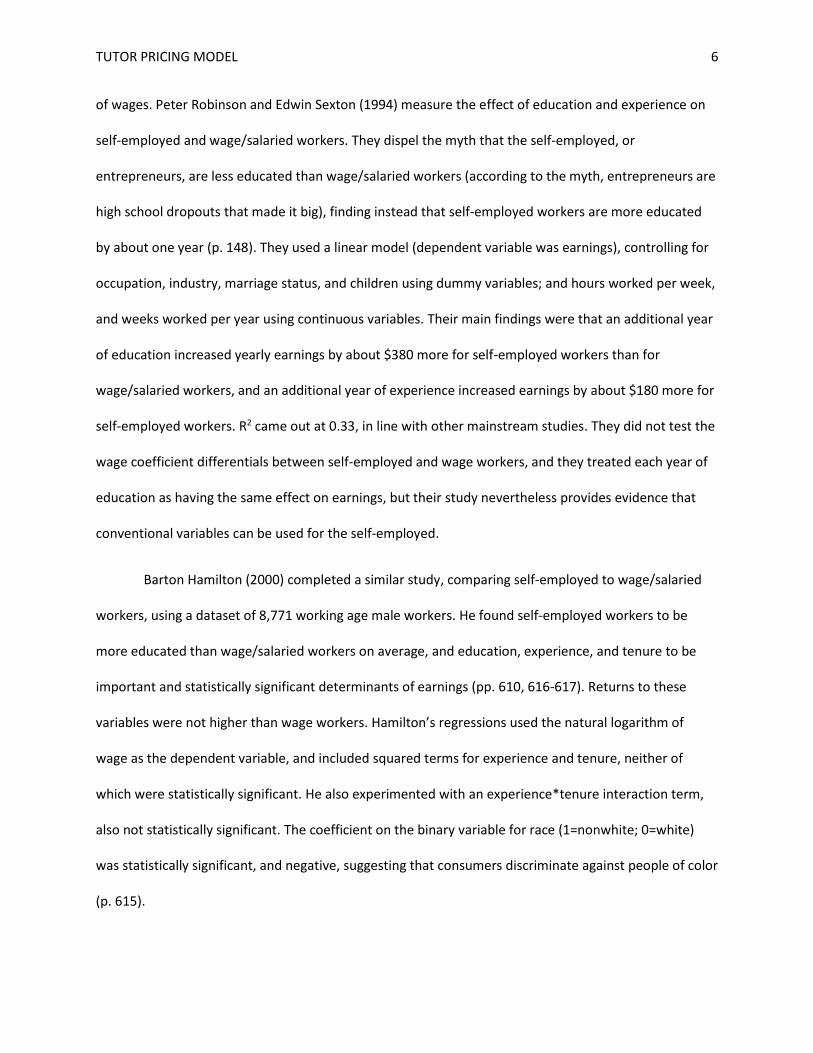
Barton Hamilton (2000) completed a similar study, comparing self-employed to wage/salaried
workers, using a dataset of 8,771 working age male workers. He found self-employed workers to be
more educated than wage/salaried workers on average, and education, experience, and tenure to be
important and statistically significant determinants of earnings (pp. 610, 616-617). Returns to these
variables were not higher than wage workers. Hamilton’s regressions used the natural logarithm of
wage as the dependent variable, and included squared terms for experience and tenure, neither of
which were statistically significant. He also experimented with an experience*tenure interaction term,
also not statistically significant. The coefficient on the binary variable for race (1=nonwhite; 0=white)
was statistically significant, and negative, suggesting that consumers discriminate against people of color
(p. 615).
TUTOR PRICING MODEL 7
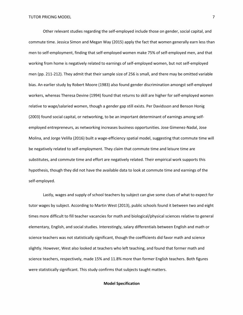
Other relevant studies regarding the self-employed include those on gender, social capital, and
commute time. Jessica Simon and Megan Way (2015) apply the fact that women generally earn less than
men to self-employment, finding that self-employed women make 75% of self-employed men, and that
working from home is negatively related to earnings of self-employed women, but not self-employed
men (pp. 211-212). They admit that their sample size of 256 is small, and there may be omitted variable
bias. An earlier study by Robert Moore (1983) also found gender discrimination amongst self-employed
workers, whereas Theresa Devine (1994) found that returns to skill are higher for self-employed women
relative to wage/salaried women, though a gender gap still exists. Per Davidsson and Benson Honig
(2003) found social capital, or networking, to be an important determinant of earnings among self-
employed entrepreneurs, as networking increases business opportunities. Jose Gimenez-Nadal, Jose
Molina, and Jorge Velilla (2016) built a wage-efficiency spatial model, suggesting that commute time will
be negatively related to self-employment. They claim that commute time and leisure time are
substitutes, and commute time and effort are negatively related. Their empirical work supports this
hypothesis, though they did not have the available data to look at commute time and earnings of the
self-employed.
Lastly, wages and supply of school teachers by subject can give some clues of what to expect for
tutor wages by subject. According to Martin West (2013), public schools found it between two and eight
times more difficult to fill teacher vacancies for math and biological/physical sciences relative to general
elementary, English, and social studies. Interestingly, salary differentials between English and math or
science teachers was not statistically significant, though the coefficients did favor math and science
slightly. However, West also looked at teachers who left teaching, and found that former math and
science teachers, respectively, made 15% and 11.8% more than former English teachers. Both figures
were statistically significant. This study confirms that subjects taught matters.
Model Specification

TUTOR PRICING MODEL 8
Freelance tutors are self-employed workers. In setting their prices, they are essentially setting
their wages. Clients, or students, then hire the tutors based on price and tutor characteristics. The
dependent variable being explained is hourly price. In order to normalize the distribution of wages and
be consistent with previous wage determination studies, the natural logarithm of wage will be used. The
independent variables determining price—based on conventional economic theory—include skills,
geographic location, job characteristics, social location (e.g. gender and race), and non-market
institutions affecting wage. Beyond conventional theory, two other wage determinants that will be
included are social capital and commute time. While personality is important, this data is unavailable for
tutors.
The variables capturing skill differentials include education, tutoring experience, and
professional certifications. A tutor with more education and experience is expected to be more skilled,
and thus higher paid, than a tutor with less. Similarly, a professional certification is expected to increase
skill and thus price. So, the coefficients on all of these variables are expected to be positive. To see the
effect of different educational degrees, education must be broken up into binary variables: some high
school, high school diploma, some college, BS/BA degree, some grad school, MS/MA degree,
Ph.D./professional student, and Ph.D./professional degree. The “some” variables are included because
there are many tutors who fall into these categories, and a college student, for example, is likely seen as
more qualified that a high school graduate not in college. To see the effect of different professional
certifications, binary variables will be included for the following certifications: teacher, tutor, social
worker, and other professional. Tutoring experience, as well as age (proxy for overall experience) is
measured in years.
Geographic location must be included because cost of living varies considerably across the
United States. Cost of living data is only available by state, so to more accurately capture this effect,

TUTOR PRICING MODEL 9
median wage by zip code is included. An area with higher wages is expected to have a higher cost of
living and therefore higher tutor prices.
Job characteristics generally refers to differing characteristics between jobs. This model is
looking at one specific job. However, as shown in the literature review, prices are expected to differ by
subject taught. Generally, technical subjects (math and science) are expected to pay more than non-
technical subjects (humanities and social studies) due to lack of tutors in these fields. Going beyond the
literature surveyed, a well-rounded tutor, or one who teaches both technical and non-technical subjects,
is likely seen as better than a tutor who teaches just one or the other. To capture these effects, binary
variables for only technical, only non-technical, and both must be defined. Because standardized testing
is widespread and very important for getting into college and grad school, an additional binary variable
for test-prep will be included. A tutor who teaches test-prep is expected to set a higher price than one
who does not.
Social location generally refers to race and gender. While race data is unavailable, data for
gender is. Conventionally, due to discrimination, women are expected to earn less than men. An
interaction variable between gender and experience will also be included as women may earn less than
men per additional year of experience (Johnson, 2001 p. 16349). Women may be seen, however, equally
as competent as men regarding teaching ability. As explained in the lit review, one study actually found
that women were entering self-employment in order to escape the gender wage gap (Devine, 1994).
Thus, gender variables may end up being unimportant.
Non-market institutions usually include trade unions and minimum wage laws. Freelance tutors
are not unionized, and minimum wage laws actually do not apply to self-employed workers (Banaian,
2013). Moreover, any effect minimum wage laws have on general wages would already be included in
the median income variable, supporting the expected positive effect of median income.
TUTOR PRICING MODEL 10
To capture the non-conventional determinants, population density by zip code will be included.
While not perfect, the higher the population density, the greater one’s ability to network (social capital).
Additionally, denser areas are expected to have higher traffic and therefore longer commutes. Both
effects suggest that the higher the population density, the higher the wages.
This discussion suggests the following model:
lnPricei = β0 + β1Expi + β2Agei + β3Cert_Teachi + β4Cert_Tutori + β5Cert_Soci + β6Cert_Profi + γ1HSi +
γ2Some_BSi + γ3BSi + γ4Some_MSi + γ5MSi + γ6Some_Profi + γ7Profi + δ1Incomei + δ2PopDensi + α1Techi +
α2Nontechi + α3Testprepi + η1fei + η2expfei+ ui
To escape the dummy variable trap, Versatilei and Some_HSi were left out, and will thus be part of the
intercept. The precise definitions of the variables will be discussed in the next section.
In addition to the mixed work around gender, and the lack of theory around including a variable
for both technical and nontechnical, one problem that may occur with including so many variables is
multicollinearity. It also may be problematic to include different dummy variables for different
certifications, as well as the “in-between” education variables (e.g. Some_MS). These issues, and more,
will be taken up in next sections.
Data
We have access to data from two tutor directories: WyzAnt.com (WyzAnt) and
TheKnowledgeRoundtable.com (KnowRo). The WyzAnt data set contains about 70,000 tutors, while the
KnowRo data set contains about 2100 tutors. Although it has more rows, the WyzAnt data set lacks
many variables we expect from theory to be important, including years of experience, certifications,
education, gender, and age. Since the KnowRo data set includes all the variables needed for our model,
it will be used in the analysis below. Note that this data is not publicly available; one of the authors is
the manager of KnowRo. The KnowRo data set is then supplemented by census data in order to map
TUTOR PRICING MODEL 11
income and population density to each tutor by zipcode (Population Studies Center, 2010; Bittner,
2014).
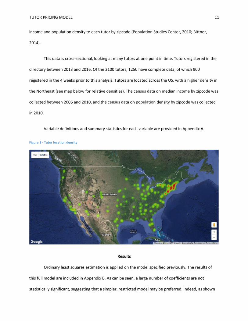
This data is cross-sectional, looking at many tutors at one point in time. Tutors registered in the
directory between 2013 and 2016. Of the 2100 tutors, 1250 have complete data, of which 900
registered in the 4 weeks prior to this analysis. Tutors are located across the US, with a higher density in
the Northeast (see map below for relative densities). The census data on median income by zipcode was
collected between 2006 and 2010, and the census data on population density by zipcode was collected
in 2010.
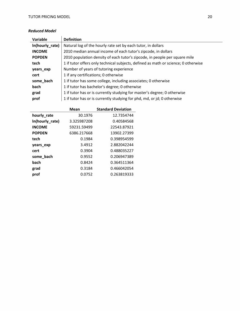
Variable definitions and summary statistics for each variable are provided in Appendix A.
Figure 1 - Tutor location density
Results
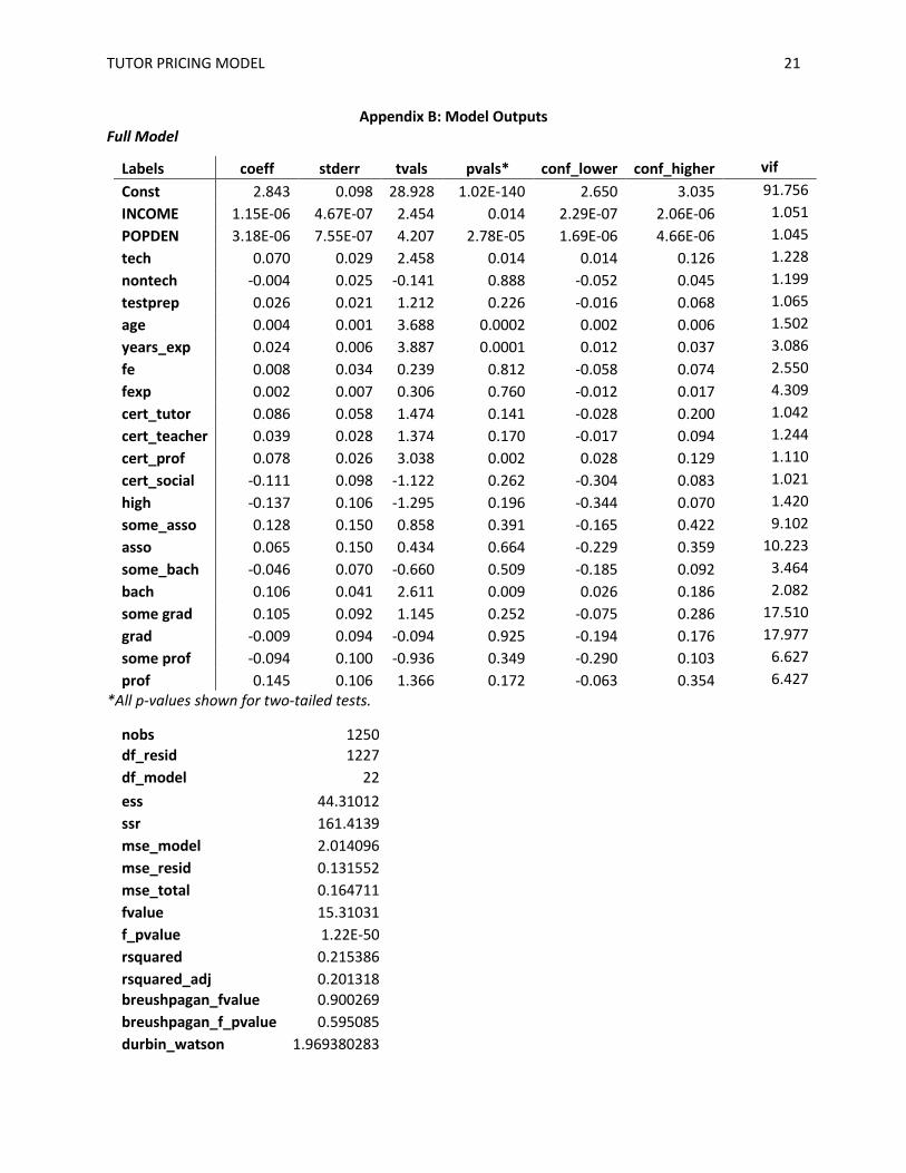
Ordinary least squares estimation is applied on the model specified previously. The results of
this full model are included in Appendix B. As can be seen, a large number of coefficients are not
statistically significant, suggesting that a simpler, restricted model may be preferred. Indeed, as shown
TUTOR PRICING MODEL 12
in the next subsection, an F-test of a model with 13 restrictions indicates that a vastly simpler model is in
fact preferred. Interpretations will be made on this simpler model.
Model Selection
The alternate model below is considered. This model is simpler in two ways: first, the
certification variables are combined as well as the education variables; second, the model restricts
variables for age, nontechnical subjects, test prep, gender, and interaction of gender with years of
experience to be zero. Thus, this model simultaneously tests whether greater detail in certifications and
education help explain more variance in hourly rate and whether gender, age, and certain subject
offerings have any explanatory power. The decision to combine education and certification variables for
this test was driven by concerns about multicollinearity. The variable Some_BS was kept due to the
significant percentage of tutors who are either current college students or associate’s degree holders.
The decision to test significance of nontechnical subjects, test prep, gender, and interaction of gender
with years of experience was driven by low p-values on these variables’ parameter estimates in the full
model and by weak theoretical justification. The decision to test significance of age, despite its
parameter estimate having a low p-value, was driven by weak theoretical justification, namely the
concern that years of tutoring experience would capture the same effect and do so more directly.
lnPricei = β0 + β1Expi + β7Certi + γ8Some_BSi + γ9BSi + γ10MSi + γ11Profi + δ1Incomei + δ2PopDensi + α1Techi
+ ui
Note that this model does not simply restrict by setting coefficients to zero; Cert and the
education variables are logical ORs of variables defined in the full model. Variable definitions and
summary statistics are provided in Appendix A. Coefficients and model statistics are provided in
Appendix B.

TUTOR PRICING MODEL 13
This simpler model is compared to the full model using an F-test. The results of this test are
presented below.
H0: The reduced model explains the same or more of the variance in hourly rate as does the full model. HA: The full model explains more of the variance in hourly rate than does the reduced model.
F-test: full model vs reduced
model ESSu 44.31012244 Alpha 0.05 ESSr 41.88060033 Fvalue 1.421788165 RSSu 161.413916 Fcrit 1.728123043 J 13 F_pvalue 0.141951412 n 1250 Reject H0? Fail to Reject k_u 22 Conclusion Accept Reduced Model
Failing to reject the null hypothesis is a surprising result, as it suggests that many factors that are
significant wage determinants in the general labor market and even the general self-employed labor
market are not significant in the self-employed tutor labor market. However, restricting so many
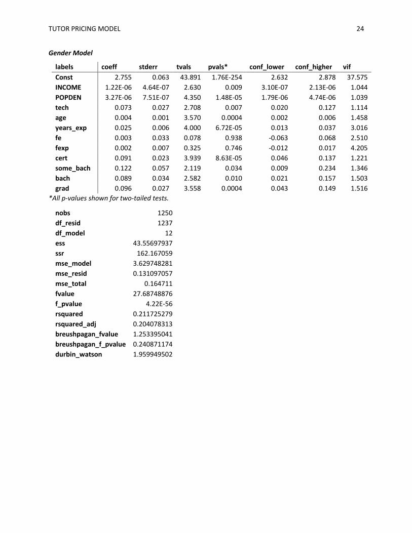
variables in one test may drown out explanatory power of individual variables. Thus, we now test this
reduced model against models in which age is included and gender and its interaction with years of
experience are included.
H0: Coefficient of Age = 0 HA: Coefficient of Age ≠ 0
F-test: age model vs reduced
model ESSu 43.51164457 Alpha 0.05 ESSr 41.88060033 Fvalue 12.46818938 RSSu 162.2123938 Fcrit 3.848968989 J 1 F_pvalue 0.000429121 n 1250 Reject H0? Yes k_u 10 Conclusion Accept Age Model
H0: 𝜂1 = 0, 𝜂2 = 0

TUTOR PRICING MODEL 14
HA: 𝜂1 ≠ 0, 𝜂2 ≠ 0
F-test: gender model vs age model ESSu 43.55697937 Alpha 0.05 ESSr 43.51164457 Fvalue 0.173045298 RSSu 162.167059 Fcrit 3.002993103 J 2 F_pvalue 0.841119855 n 1250 Reject H0? Fail to Reject k_u 12 Conclusion Accept Age Model
These tests suggest that Age should be included in the model, but not fe or expfe. The
significance of age despite the presence of the seemingly redundant factor of years of experience can be
explained by the fact that, for example, some middle-aged professionals need to earn a high rate
because of their life circumstances, but may have less tutoring experience than a college student who
has tutored their peers for several years.
Our final model is as follows.
lnPricei = β0 + β1Expi + β2Agei + β7Certi + γ8Some_BSi + γ9BSi + γ10MSi + γ11Profi + δ1Incomei + δ2PopDensi +
α1Techi + ui
It should be noted that for the final reduced model, we fail to reject the null hypothesis that
error variances are constant via the Breusch-Pagan test (p-values presented in Appendix B). Thus, there
are no signs of heteroskedasticity. Lack of autocorrelation is also confirmed with a Durbin-Watson
statistic close to 2 (which is expected for cross-sectional data). Finally, multicollinearity was a major
issue in the full model (indicated by high variance inflation factors on many variables), but was resolved
for all variables in the final reduced model with the exception of the intercept (perhaps because 95% of
tutors have Some_Bach=1).
Model Interpretation

TUTOR PRICING MODEL 15
The final reduced model explains 21.2% of the variance in tutors’ hourly rates according to the
model’s R2 value, and is highly statistically significant (the p-value for an F-test with null hypothesis “all
coefficients=0” is 1.49x10-57). Also, as mentioned in the section above, no issues with heteroskedasticity,
autocorrelation, or multicollinearity are present. Thus, since all parameter estimates are statistically
significant at the 0.05 level (whether one-tailed or two-tailed tests are used), except for that for Prof, we
can safely and confidently interpret the model’s parameters as follows.
Variable Parameter
Parameter
Estimate Interpretation
CONST β0 2.759 When all variables are zero, a tutor will charge 𝑒2.759 =$15.78/hr. This includes the base cases of high school degree only and offering not only technical subjects.
INCOME δ1 1.21E-06 A $10,000 increase in median annual income of a tutor’s zipcode results in an hourly rate increase of 1.21%, all else constant.
POPDEN δ2 3.24E-06 A 10,000 person per square mile increase in population density of a tutor’s zipcode results in an hourly rate increase of 3.24%, all else constant.
tech α1 0.070
Tutors offering only technical subjects charge (𝑒0.066 −1)100 = 7.25% more per hour than those who offer non-technical subjects only or both technical and nontechnical subjects, all else constant.
age β2 0.004 One additional year of age results in an hourly rate increase of 0.4%, all else constant.
years_exp β1 0.026 One additional year of tutoring experience results in an hourly rate increase of 2.6%, all else constant.
cert β7 0.092 Tutors holding at least one certification charge (𝑒0.092 −1)100 = 9.64% more per hour than those who do not hold any, all else constant.
some_bach γ8 0.122 Tutors having some college, including associates, charge (𝑒0.122 − 1)100 = 12.98% more per hour than those who only have a high school degree, all else constant.
bach γ9 0.090 Tutors having a bachelor’s degree charge (𝑒0.090 −1)100 = 9.42% more per hour than those who only have some college, all else constant.
grad γ10 0.096 Tutors having a graduate degree charge (𝑒0.096 −1)100 = 10.08% more per hour than those who only have a bachelor’s degree, all else constant.
All of these parameter estimates confirm our expectations from theory, with the exception of offering
technical subjects only. In that case, we expected tutors offering both technical and nontechnical

TUTOR PRICING MODEL 16
subjects to demand a premium over those offering only one or the other. Surprisingly, versatile tutors
charge (1 − 11+0.0725) ∗ 100% = 6.76% less than those who only offer technical subjects.
While most variables in the simple model have parameter estimates with the expected sign, it is
unexpected that estimates for the variables test prep, nontechnical subjects, gender, and interaction of
gender with years of experience do not explain a statistically significant portion of the variance in hourly
rate. This suggests additional work to be done on the importance of subjects taught. The insignificance
of gender supports Theresa Devine’s work, but also could simply be due to female tutors refusing to set
their prices lower than men. It is still possible that clients choose male tutors more than females,
something this model could not test.
Summary and Conclusions
This paper fills gaps in the academic literature and the tutoring industry by presenting the first
quantitative tutor pricing model of national scale. From a review of formal academic literature related to
wage determinants and the self-employed labor market, as well as informal literature available on
popular tutoring websites, we first identify categories of factors likely to have explanatory power as
wage determinants in the self-employed labor market, shown below. We then select specific factors for
each category that are particularly relevant for the tutoring industry and have data available.
Skills Geography
Job
Characteristics
Social
Location Unconventional
Education Median Annual
Income Technical Gender
Population
density
Years of tutoring
experience Population density Non-technical Age
Professional
certifications Test prep
Age
TUTOR PRICING MODEL 17
Our data set contains 1250 tutors from TheKnowledgeRoundtable.com, a national directory of
tutors. The tutor data set is supplemented with Census data that provides the income and population
density of each tutor’s zipcode. After comparing the statistical significance of 5 model variants, we show
that the best model is the following, where variables are as defined in Appendix A.
lnPricei = β0 + β1Expi + β2Agei + β7Certi + γ8Some_BSi + γ9BSi + γ10MSi + γ11Profi + δ1Incomei + δ2PopDensi +
α1Techi + ui
This model was estimated using Ordinary Least Squares and successfully explained 21.2% of the
variation in tutor prices. We show that the model does not suffer from issues of heteroskedasticity,
autocorrelation, or multicollinearity and thus inference can be performed.
There are two key, unexpected results. First, gender and the interaction of gender with years of
experience are not statistically significant factors determining tutor price. Tutoring thus appears to
break the mold of the gender pay gap. Second, the effects of subjects offered on tutor price are
unexpected: tutors who offer only technical subjects surprisingly charge more than versatile tutors who
offer both technical and non-technical subjects; and tutors who offer test prep do not charge more than
those who do not.
The model otherwise confirms established theories regarding wage determinants and the self-
employed labor market. Education, experience, certifications, age, income, and population density all
have a positive effect on tutor prices. Our research suggests that the model could be improved—that is,
more variation in tutor price could be explained—by collecting data on tutors’ personality traits.

TUTOR PRICING MODEL 18

TUTOR PRICING MODEL 19
Appendix A: Variable Definitions and Summary Statistics
Full Model
Variable Definition
ln(hourly_rate) Natural log of the hourly rate set by each tutor, in dollars INCOME 2010 median annual income of each tutor's zipcode, in dollars POPDEN 2010 population density of each tutor's zipcode, in people per square mile tech 1 if tutor offers only technical subjects, defined as math or science; 0 otherwise
nontech 1 if tutor offers only nontechnical subjects, defined as English, humanities, or foreign language; 0 otherwise
testprep 1 if tutor offers test prep tutoring; 0 otherwise age Age in years years_exp Number of years of tutoring experience fe 1 if female; 0 if male fexp fe*years_exp cert_tutor 1 if certified by a tutoring certification organization such as NRLA; 0 otherwise cert_teacher 1 if certified as a teacher; 0 otherwise cert_prof 1 if tutor has other related professional certifications, e.g. actuarial exams; 0 otherwise cert_social 1 if certified as a social worker; 0 otherwise high 1 if tutor has high school degree; 0 otherwise some_asso 1 if tutor has some associate degree work; 0 otherwise asso 1 if tutor has associates degree; 0 otherwise some_bach 1 if tutor has some college; 0 otherwise bach 1 if tutor has bachelor's degree; 0 otherwise some grad 1 if tutor has some master's work; 0 otherwise grad 1 if tutor has master's degree; 0 otherwise some prof 1 if tutor has some phd, md, or jd; 0 otherwise prof 1 if tutor has phd, md, or jd; 0 otherwise
Mean Standard Deviation Mean Standard Deviation
hourly_rate 30.198 12.735 cert_teacher 0.210 0.407 ln(hourly_rate) 3.326 0.406 cert_prof 0.226 0.419 INCOME 59231.595 22543.879 cert_social 0.011 0.105 POPDEN 6386.218 13902.274 high 0.986 0.116 tech 0.198 0.399 some_asso 0.955 0.207 nontech 0.286 0.452 asso 0.950 0.219 testprep 0.582 0.493 some_bach 0.920 0.271 age 29.798 11.983 bach 0.842 0.365 years_exp 3.491 2.882 some grad 0.318 0.466 fe 0.621 0.485 grad 0.306 0.461 fexp 2.195 2.852 some prof 0.075 0.264 cert_tutor 0.034 0.180 prof 0.064 0.245
TUTOR PRICING MODEL 20
Reduced Model
Variable Definition
ln(hourly_rate) Natural log of the hourly rate set by each tutor, in dollars INCOME 2010 median annual income of each tutor's zipcode, in dollars POPDEN 2010 population density of each tutor's zipcode, in people per square mile tech 1 if tutor offers only technical subjects, defined as math or science; 0 otherwise years_exp Number of years of tutoring experience cert 1 if any certifications; 0 otherwise some_bach 1 if tutor has some college, including associates; 0 otherwise bach 1 if tutor has bachelor's degree; 0 otherwise grad 1 if tutor has or is currently studying for master's degree; 0 otherwise prof 1 if tutor has or is currently studying for phd, md, or jd; 0 otherwise
Mean Standard Deviation
hourly_rate 30.1976 12.7354744 ln(hourly_rate) 3.325987208 0.40584568 INCOME 59231.59499 22543.87921 POPDEN 6386.217668 13902.27399 tech 0.1984 0.398954599 years_exp 3.4912 2.882042244 cert 0.3904 0.488035227 some_bach 0.9552 0.206947389 bach 0.8424 0.364511364 grad 0.3184 0.466042054 prof 0.0752 0.263819333
TUTOR PRICING MODEL 21
Appendix B: Model Outputs
Full Model
Labels coeff stderr tvals pvals* conf_lower conf_higher vif
Const 2.843 0.098 28.928 1.02E-140 2.650 3.035 91.756 INCOME 1.15E-06 4.67E-07 2.454 0.014 2.29E-07 2.06E-06 1.051 POPDEN 3.18E-06 7.55E-07 4.207 2.78E-05 1.69E-06 4.66E-06 1.045 tech 0.070 0.029 2.458 0.014 0.014 0.126 1.228 nontech -0.004 0.025 -0.141 0.888 -0.052 0.045 1.199 testprep 0.026 0.021 1.212 0.226 -0.016 0.068 1.065 age 0.004 0.001 3.688 0.0002 0.002 0.006 1.502 years_exp 0.024 0.006 3.887 0.0001 0.012 0.037 3.086 fe 0.008 0.034 0.239 0.812 -0.058 0.074 2.550 fexp 0.002 0.007 0.306 0.760 -0.012 0.017 4.309 cert_tutor 0.086 0.058 1.474 0.141 -0.028 0.200 1.042 cert_teacher 0.039 0.028 1.374 0.170 -0.017 0.094 1.244 cert_prof 0.078 0.026 3.038 0.002 0.028 0.129 1.110 cert_social -0.111 0.098 -1.122 0.262 -0.304 0.083 1.021 high -0.137 0.106 -1.295 0.196 -0.344 0.070 1.420 some_asso 0.128 0.150 0.858 0.391 -0.165 0.422 9.102 asso 0.065 0.150 0.434 0.664 -0.229 0.359 10.223 some_bach -0.046 0.070 -0.660 0.509 -0.185 0.092 3.464 bach 0.106 0.041 2.611 0.009 0.026 0.186 2.082 some grad 0.105 0.092 1.145 0.252 -0.075 0.286 17.510 grad -0.009 0.094 -0.094 0.925 -0.194 0.176 17.977 some prof -0.094 0.100 -0.936 0.349 -0.290 0.103 6.627 prof 0.145 0.106 1.366 0.172 -0.063 0.354 6.427
*All p-values shown for two-tailed tests.
nobs 1250 df_resid 1227 df_model 22 ess 44.31012 ssr 161.4139 mse_model 2.014096 mse_resid 0.131552 mse_total 0.164711 fvalue 15.31031 f_pvalue 1.22E-50 rsquared 0.215386 rsquared_adj 0.201318 breushpagan_fvalue 0.900269 breushpagan_f_pvalue 0.595085 durbin_watson 1.969380283
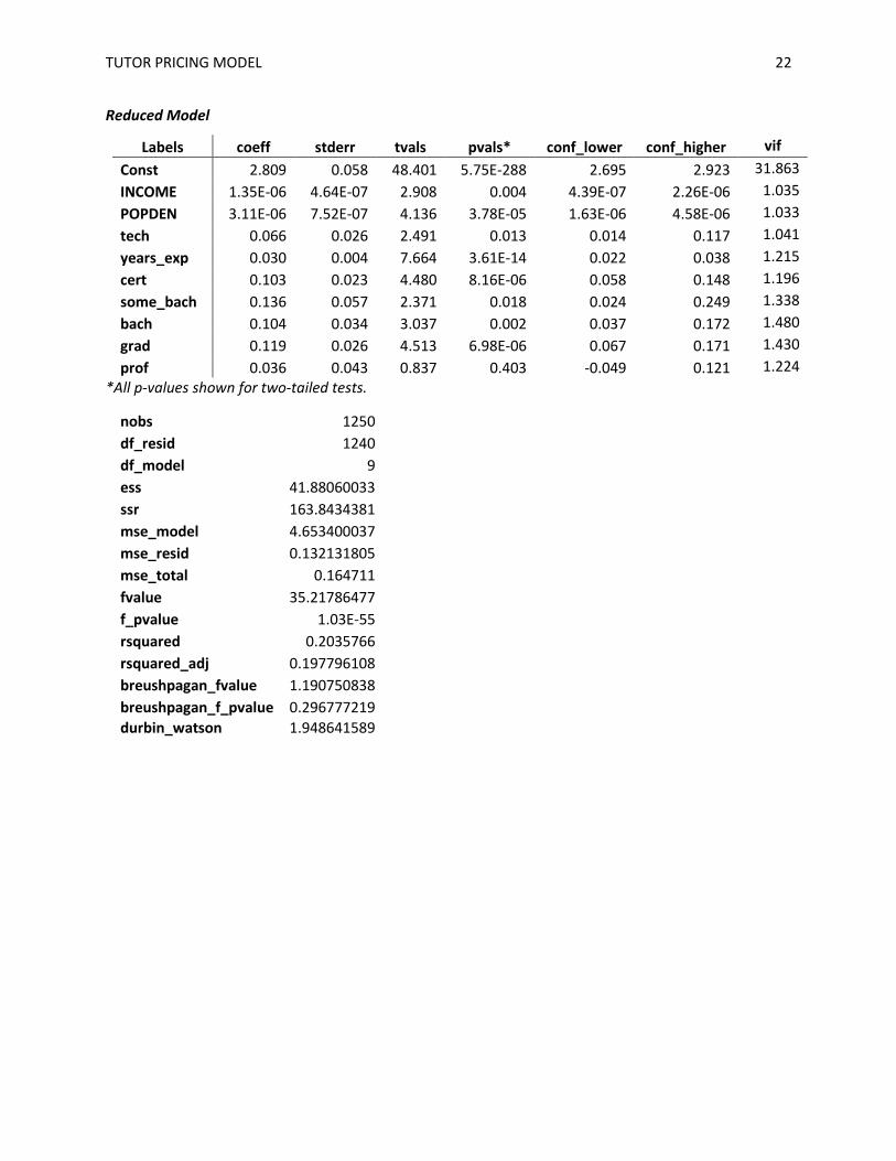
TUTOR PRICING MODEL 22
Reduced Model
Labels coeff stderr tvals pvals* conf_lower conf_higher vif
Const 2.809 0.058 48.401 5.75E-288 2.695 2.923 31.863 INCOME 1.35E-06 4.64E-07 2.908 0.004 4.39E-07 2.26E-06 1.035 POPDEN 3.11E-06 7.52E-07 4.136 3.78E-05 1.63E-06 4.58E-06 1.033 tech 0.066 0.026 2.491 0.013 0.014 0.117 1.041 years_exp 0.030 0.004 7.664 3.61E-14 0.022 0.038 1.215 cert 0.103 0.023 4.480 8.16E-06 0.058 0.148 1.196 some_bach 0.136 0.057 2.371 0.018 0.024 0.249 1.338 bach 0.104 0.034 3.037 0.002 0.037 0.172 1.480 grad 0.119 0.026 4.513 6.98E-06 0.067 0.171 1.430 prof 0.036 0.043 0.837 0.403 -0.049 0.121 1.224
*All p-values shown for two-tailed tests.
nobs 1250 df_resid 1240 df_model 9 ess 41.88060033 ssr 163.8434381 mse_model 4.653400037 mse_resid 0.132131805 mse_total 0.164711 fvalue 35.21786477 f_pvalue 1.03E-55 rsquared 0.2035766 rsquared_adj 0.197796108 breushpagan_fvalue 1.190750838 breushpagan_f_pvalue 0.296777219 durbin_watson 1.948641589

TUTOR PRICING MODEL 23
Age Model (Final Reduced Model)
Labels coeff stderr tvals pvals* conf_lower conf_higher vif
Const 2.759 0.059 46.371 5.17E-273 2.642 2.875 33.794 INCOME 1.21E-06 4.64E-07 2.614 0.009 3.02E-07 2.12E-06 1.042 POPDEN 3.24E-06 7.49E-07 4.327 1.63E-05 1.77E-06 4.71E-06 1.036 tech 0.070 0.026 2.664 0.008 0.018 0.121 1.043 age 0.004 0.001 3.530 0.0004 0.002 0.006 1.439 years_exp 0.026 0.004 6.483 1.30E-10 0.018 0.034 1.308 cert 0.092 0.023 3.975 7.44E-05 0.047 0.137 1.218 some_bach 0.122 0.057 2.127 0.034 0.009 0.235 1.344 bach 0.090 0.034 2.609 0.009 0.022 0.157 1.501 grad 0.096 0.027 3.558 0.0004 0.043 0.149 1.516 prof 0.032 0.043 0.737 0.461 -0.053 0.116 1.225
*All p-values shown for two-tailed tests.
nobs 1250 df_resid 1239 df_model 10 ess 43.51164457 ssr 162.2123938 mse_model 4.351164457 mse_resid 0.130922029 mse_total 0.164711 fvalue 33.23477716 f_pvalue 1.49E-57 rsquared 0.211504912 rsquared_adj 0.205140948 breushpagan_fvalue 1.199005014 breushpagan_f_pvalue 0.287010967 durbin_watson 1.958830888
TUTOR PRICING MODEL 24
Gender Model
labels coeff stderr tvals pvals* conf_lower conf_higher vif
Const 2.755 0.063 43.891 1.76E-254 2.632 2.878 37.575 INCOME 1.22E-06 4.64E-07 2.630 0.009 3.10E-07 2.13E-06 1.044 POPDEN 3.27E-06 7.51E-07 4.350 1.48E-05 1.79E-06 4.74E-06 1.039 tech 0.073 0.027 2.708 0.007 0.020 0.127 1.114 age 0.004 0.001 3.570 0.0004 0.002 0.006 1.458 years_exp 0.025 0.006 4.000 6.72E-05 0.013 0.037 3.016 fe 0.003 0.033 0.078 0.938 -0.063 0.068 2.510 fexp 0.002 0.007 0.325 0.746 -0.012 0.017 4.205 cert 0.091 0.023 3.939 8.63E-05 0.046 0.137 1.221 some_bach 0.122 0.057 2.119 0.034 0.009 0.234 1.346 bach 0.089 0.034 2.582 0.010 0.021 0.157 1.503 grad 0.096 0.027 3.558 0.0004 0.043 0.149 1.516
*All p-values shown for two-tailed tests.
nobs 1250 df_resid 1237 df_model 12 ess 43.55697937 ssr 162.167059 mse_model 3.629748281 mse_resid 0.131097057 mse_total 0.164711 fvalue 27.68748876 f_pvalue 4.22E-56 rsquared 0.211725279 rsquared_adj 0.204078313 breushpagan_fvalue 1.253395041 breushpagan_f_pvalue 0.240871174 durbin_watson 1.959949502

TUTOR PRICING MODEL 25
References
Altonji, J. G., & Blank, R. M. (1999). Race and gender in the labor market. Handbook of Labor
Economics, 3C, 3143-3260. Retrieved from /z-wcorg/ database. Banaian, K. (2013, February 19). The minimum wage for the self-employed is $0.00. Retrieved April 25,
2016, from http://www.americanexperiment.org/blog/201302/the-minimum-wage-for-the-self-employed-is-000
Bittner, J. (2014, January 06). Free US Population Density And Unemployment Rate By Zip Code.
Retrieved April 27, 2016, from https://blog.splitwise.com/2014/01/06/free-us-population-density-and-unemployment-rate-by-zip-code/
Bowles, S., Gintis, H., & Osborne, M. (2000). The Determinants of Earnings: Skills, Preferences, and
Schooling. ScholarWorks@UMass Amherst. Bowles, S., Gintis, H., & Osborne, M. (2001). Incentive-enhancing preferences: Personality, behavior, and
earnings. The American Economic Review, 91(2), 155-158. Retrieved from /z-proquest_abi_global/ database.
Devine, T. J. (1994). Changes in wage-and-salary returns to skill and the recent rise in female self-
employment. The American Economic Review, 84(2), 108-113. Retrieved from /z-proquest_abi_global/ database.
Duncan, G. J., & Dunifon, R. (2012). Introduction to “’soft-skills’ and long-run labor market
success”. Research in Labor Economics, 35, 309-312. Gimenez-Nadal, J. I., Molina, J. A., & Velilla, J. (2016). A wage-efficiency spatial model for US self-
employed workers. Bonn: IZA. Hamermesh, D., & Biddle, J. (1994). Beauty and the labor market. American Economic Review, 84(5),
1174-1194. Retrieved from /z-proquest_abi_global/ database. Hamilton, B. H. (2000). Does entrepreneurship pay? an empirical analysis of the returns to self-
employment. Journal of Political Economy, 108, 604-631. Retrieved from /z-wcorg/ database. Honig, B., & Davidsson, P. (2003). The role of social and human capital among nascent
entrepreneurs. Journal of Business Venturing, 18, 301-331. Retrieved from /ebsco_bth/ database.
How Much Should I Charge For Tutoring? (2015). Retrieved April 25, 2016, from
https://www.appointment-plus.com/articles/how_much_to_charge_for_tutoring_sessions.php Johnson, G. (2001). Wage differentials and structure. In N. J. S. B. Baltes (Ed.), International encyclopedia
of the social & behavioral sciences (pp. 16345-16350). Oxford: Pergamon. doi: http://dx.doi.org/10.1016/B0-08-043076-7/02285-3

TUTOR PRICING MODEL 26
Moore, R. L. (1983). Employer discrimination: Evidence from self-employed workers. The Review of
Economics and Statistics,65(3), 496-501. Retrieved from http://www.jstor.org/stable/1924197?seq=1#page_scan_tab_contents
Rand, J. (2015, February 24). How Much to Charge for Tutoring. Retrieved April 25, 2016, from
https://www.theknowledgeroundtable.com/how-much-to-charge-for-tutoring/ Rand, J. (2016). [Tutor price and demographic data from Knowledge Roundtable]. Unpublished raw data. Rate and Policies. (2016). Retrieved April 25, 2016, from
https://www.wyzant.com/Tutor/RateAndPolicies.aspx Robinson, P. B., & Sexton, E. A. (1994). The effect of education and experience on self-employment
success. Journal of Business Venturing, 9(2), 141-156. Retrieved from /z-proquest_abi_global/ database.
Schultz, T. W. (1975). The value of the ability to deal with disequilibria. Journal of Economic
Literature, 13(3), 827-847. Retrieved from http://silk.library.umass.edu/login?url=http://search.ebscohost.com/login.aspx?direct=true&db=bth&AN=5310693&site=ehost-live&scope=site
Simon, J., & Way, M. M. (2015). Working from home and the gender gap in earnings for self-employed
US millennials. Gender in Management: An International Journal, 30(3), 206-224. Retrieved from /z-wcorg/ database.
The Tutor Guide: Tutoring Fees. (2013, April 24). Retrieved April 25, 2016, from
http://www.care.com/tutoring-tutoring-fees-p1145-q3356.html Viinikainen, J., Kokko, K., Pulkkinen, L., & Pehkonen, J. (2010). Personality and labour market income:
Evidence from longitudinal data. Labour, 24(2), 201-220. Retrieved from /wiley_onlib/ database. Warkentin, S. (2015, June 4). How Much Should Tutoring Cost? Retrieved April 25, 2016, from
https://www.angieslist.com/articles/how-much-should-tutoring-cost.htm West, M. R. (2013, April 17). Do Math and Science Teachers Earn More Outside of Education? (Tech. No.
17). Retrieved April 25, 2016, from The Brookings Institution website: http://www.brookings.edu/research/papers/2013/04/17-math-science-teachers-west
Zip Code Characteristics: Mean and Median Household Income. (2010). Retrieved April 27, 2016, from
the Population Studies Center, Institute for Social Research, University of Michigan website http://www.psc.isr.umich.edu/dis/census/Features/tract2zip/