School of Economics and Management

Department of Economics

The Impacts of FDI on Productivity and Economic

Growth: A Comparative Perspective

Master Thesis, Spring 2010

Author: Cem Tintin Supervisor: Klas Fregert

2

TABLE OF CO*TE*TS

ABSTRACT ............................................................................................................................. 3

DEDICATIO* ......................................................................................................................... 4

ACK*OWLEDGEME*TS .................................................................................................... 5

LIST OF TABLES A*D FIGURES ...................................................................................... 6

LIST OF ABBREVIATIO*S A*D ACRO*YMS ............................................................... 7

1. I*TRODUCTIO* ............................................................................................................... 8

2. LITERATURE REVIEW ................................................................................................. 10

3. THEORETICAL BACKGROU*D A*D EMPIRICAL MODELS ............................. 14

3.1 Definitions of FDI .......................................................................................................... 14

3.2 The Impacts of FDI in Economic Growth Theory ......................................................... 15

3.2.1 The Impact of FDI on Capital Accumulation: Capital Widening ................ 15

3.2.2 The Impact of FDI on Productivity: Capital Deepening .............................. 16

3.3 Empirical Models .......................................................................................................... 19

3.3.1 Empirical Models: The Impact of FDI on Economic Growth ....................... 19

3.3.2 Empirical Models: The Impact of FDI on Productivity ................................. 23

4. DATA .................................................................................................................................. 25

4.1 Sources and Description of Data .................................................................................... 25

4.2 Definition of Samples .................................................................................................... 27

5. METHODS A*D ESTIMATIO* RESULTS ................................................................. 28

5.1 Methods ......................................................................................................................... 29

5.2 Panel Unit Root Tests .................................................................................................... 29

5.3 Panel Cointegration Tests ............................................................................................. 32

5.4 Estimation Method and Results .................................................................................... 35

5.4.1 Estimation Method .................................................................................................. 35

5.4.2 Estimation Results ................................................................................................... 37

5.4.2.1 Estimation Results: The Impact of FDI on Economic Growth ................... 37

5.4.2.2 Estimation Results: The Impact of FDI on Productivity ............................ 41

6. CO*CLUSIO*S A*D IMPLICATIO*S ....................................................................... 43

REFERE*CES ...................................................................................................................... 47

APPE*DICES ........................................................................................................................ 53

3

ABSTRACT

This study investigates the impacts of FDI on productivity and economic growth in

comparative perspective by using two samples, namely “developing” and “developed”

countries. The study employs panel cointegration and panel estimation methods. The panel

cointegration test results indicate that there are long-run relations between “FDI and

productivity”, and “FDI and economic growth” variables. The study’s main findings show

that FDI triggers (labor) productivity and economic growth in a positive way but at different

degrees. Nonetheless, the magnitudes of these effects differ across developing and developed

countries. Moreover, the findings testify that the impacts of FDI on productivity and

economic growth can be improved with high labor quality. Finally, it is analyzed that higher

openness and macroeconomic stability might be other important factors in assessing the

positive impacts of FDI concerning economic growth.

Key Words: Foreign Direct Investment, Productivity, Economic Growth, Panel

Cointegration, Panel Estimation.

4

To My Family

5

ACK*OWLEDGEME*TS

I would like to thank my supervisor Associate Professor Klas Fregert for his invaluable

comments and guidance throughout the writing of this thesis. Also, I would like to thank the

Swedish Institute for financial support during my studies in Sweden. A special word of thanks

goes to the members of my family who have encouraged and unconditionally supported me

throughout all my studies.

6

LIST OF TABLES A*D FIGURES

TABLES

Table 1: Summary of Some Selected Empirical Studies on FDI ............................................. 13

Table 2: Definitions of the Dependent and Independent Variables .......................................... 24

Table 3: Expected Signs of the Coefficients of Independent Variables .................................. 24

Table 4: Summary of Data Sources and Description .............................................................. 27

Table 5: Sample Groups .......................................................................................................... 28

Table 6: Estimation Results with Annual Data and 5-year Averages ...................................... 55

Table 7: Employed Tests and Methods .................................................................................... 29

Table 8: Panel Unit Root Test Results...................................................................................... 56

Table 9: The Johansen-Fisher Panel Cointegration Test Results: Fisher Statistic

From Trace Test ........................................................................................................................ 57

Table 10: The Johansen-Fisher Panel Cointegration Test Results: Fisher Statistic

From Max-Eigen Test ............................................................................................................... 58

Table 11: Estimation Results of Models 1 to 4 ........................................................................ 37

Table 12: Estimation Results of Models 5 and 6 ..................................................................... 41

Table 13: Estimation Results of Models 7 and 8 ...................................................................... 42

FIGURES

Figure 1: The Role of Capital in Economic Growth Models .................................................. 18

Figure 2: Openness and FDI Relation in Developing Countries .............................................. 59

7

LIST OF ABBREVIATIO*S A*D ACRO*YMS

ADF Augmented Dickey-Fuller

ARDL Autoregressive Distributed Lag

DOLS Dynamic Ordinary Least Squares

Eq. Equation

FDI Foreign Direct Investment

FMOLS Fully modified Ordinary Least Squares

G1 Developing Countries Sample

G2 Developed Countries Sample

GDP Gross Domestic Product

GSP Gross State Product

IFS International Financial Statistics

IMF International Monetary Fund

INF Inflation Rate

IPS Im-Peseran-Shin

LP Labor Productivity

LQ Labor Quality

OECD Organisation for Economic Co-operation and Development

OLS Ordinary Least Squares

OPEN Openness Index

PGDP Per capita Gross Domestic Product

TFP Total Factor Productivity

TNE Transnational Enterprises

UK United Kingdom

UNCTAD United Nations Conference on Trade and Development.

UNDP United Nations Development Programme

USA United States of America

VAR Vector Autoregression

8

1. I*TRODUCTIO*

The globalization process, which aims to reduce all kind of barriers across countries, has

fostered the physical and financial capital flows tremendously in the last thirty years.

Although physical capital is a less mobile factor relative to financial capital, the amounts of

FDI inflows and stocks in both developing and developed counties have been rocketed up

since 1980s due to reduced barriers for foreign direct investors. In particular, the collapse of

Soviet Union and the open market oriented policies followed by developing countries such as

China and India have been accelerated the pace of direct investments which led to increase in

the share of FDI stock as percentage of GDP in all countries.1

FDI has been increasingly seen as an important stimulus for productivity and economic

growth both for developing and developed countries. According to OECD; “FDI triggers

technology spillovers, assists human capital formation, contributes to international trade

integration, helps create a more competitive business environment, and enhances enterprise

development.” (OECD, 2002, p.5). According to the Solow economic growth model; the

capital stock of a country enlarges due to FDI inflows henceforth this country would

experience economic growth in the short run which is known as capital widening. On the

other hand, endogenous growth models adds a further dimension that the latest technology

and managerial skills in developed countries can be transferred to all countries via FDI which

would also trigger productivity and economic growth in host countries which is defined as

capital deepening. In a nutshell, economic theory predicts that FDI triggers productivity and

economic growth by different channels.

In this regard, this study aims to investigate the prediction of economic theory by analyzing

the impacts of FDI on productivity and economic growth in comparative perspective by using

two samples namely “developing” and “developed” countries. Because empirical findings of

previous studies are somewhat mixed about the impacts of FDI on productivity and economic

growth in different countries (Johnson, 2006, p.3). In particular, the results differ according to

the method of analysis that researchers employ and selected sample countries for the analysis.

Moreover, the findings point out that the impacts of FDI might differ remarkably between

1 For example, in 1990 “inward FDI stock of all countries as a percentage total world GDP” was 8.77, as of 2008

this figure reached to 24.38, which is a historical record (World Investment Report, 2009).

9

developed and developing countries which have different economic and institutional

structures. Therefore, this subject needs to be analyzed with different models and samples to

gain further insights about the impacts of FDI on productivity and economic growth.

The study mainly uses panel data approach in analyzing the impacts of FDI on productivity

and economic growth and differs from other studies in four respects. First of all, the study

has two sample country groups namely “developing” and “developed” countries. Therefore,

in the analysis it would be clarified whether the impacts of FDI differ remarkably between

developing and developed country groups. Secondly, the study uses three additional

explanatory variables (labor quality index, openness, inflation) in addition to main “FDI”

explanatory variable. It is the first time that the study employs the “labor quality index” as an

absorption capacity variable, which is constructed by Bonthuis (2010). Thirdly, the study uses

two productivity measures “labor productivity and total factor productivity” in the analysis

which increases the robustness of the analysis and adds additional insights into the discussion.

Finally, the study employs recent panel unit root, panel cointegration and panel estimation

methods in the analysis such as the IPS, Breitung panel unit root and Johansen-Fisher panel

cointegration tests.

The main findings of the study show that there are cointegration relations between “FDI and

productivity” and “FDI and economic growth” variables. Moreover, the findings suggest that

FDI enhances (labor) productivity and economic growth in a positive way but at different

degrees. Besides, the magnitudes of these impacts differ across developing and developed

countries. Notably, the findings testify the importance of absorption capacity that the impacts

of FDI on productivity and economic growth can be improved with high labor quality.

Finally, it is argued that openness and macroeconomic stability might be other important

factors in assessing the positive impacts of FDI concerning economic growth.

The organization of the study is as follows. After this short introduction, section 2 provides a

brief literature review and discusses other researchers’ main findings. Section 3 revisits the

economic growth models with attaining special importance to FDI and discusses how FDI can

be integrated into the growth models. It also derives and presents the formal models that are

used in the analysis. Section 4 explains sources and transformation of data. And it presents the

sample groups. Section 5 documents the results of the unit root tests, cointegration tests and

model estimations. In addition, it discusses the findings of the analysis in the light of

10

economic theory and previous studies. Section 6 summarizes the findings of the study and

concludes by adding policy implications for policy makers.

2. LITERATURE REVIEW

In this section, we present and discuss some selected empirical studies regarding the impacts

of FDI on productivity and economic growth in which authors used similar methods and

variables to our study. Then, Table 1 documents the summary of some selected studies.

In a benchmark article for our study, Johnson (2006) examines whether FDI has a positive

effect on economic growth by triggering technology spillovers and physical capital

accumulation. He uses a panel dataset compromising 90 developed and developing countries

between 1980 and 2002 period. In his regression model, he uses the “annual growth rate of

real per capita GDP” as the dependent variable and “average inward FDI stock as a share in

GDP” as the main independent variable. In addition, he uses some control variables which are

domestic investments, average years of schooling and interaction term of schooling & FDI,

and economic freedom index. He performs the empirical analysis by using OLS method both

for cross-section and panel data and finds out that “FDI enhances economic growth in

developing economies but not in developed economies” (Johnson, 2006, p.43). He also

estimates positive coefficients for the schooling variable and its interaction term which imply

the importance of absorption capacity in assessing the positive impacts of FDI.

Neuhaus (2006) makes an important contribution to the literature of FDI-led growth. In his

book, he formally introduces the FDI discussion into the endogenous growth models. In

addition, he makes an empirical investigation by using the data of 13 Central and Eastern

Europe Countries over the period from 1991 to 2002. While constructing his empirical model,

he substitutes the “human capital variable” of Mankiw, Romer and Weil (1992) growth model

with “FDI variable”. Furthermore, he includes some additional explanatory variables such as

the lag of per capita income, trade openness, inflation volatility, government consumption,

government balance, and domestic investment to improve the explanatory power of his

model. And he uses the growth rate of per capita income as the dependent variable. He runs

his ARDL (autoregressive distributed lag) type regression model by using pooled mean group

estimation method. As a result of estimations, he concludes that “FDI had a significant

11

positive impact on the rate of economic growth in Central and Eastern Europe Countries”

(Neuhaus, 2006, p.81). Moreover, he claims that FDI is an important determinant of growth

especially for transition economies. Therefore, he supports pro-FDI policies of governments

to attract more FDI inflows for growth and development.

Olofsdotter (1998) finds evidence that FDI has positive impacts on growth by using the data

of 50 countries over the period 1980-1990. Remarkably, she has considered the absorption

capability of the host countries by using two variables “degree of property-right protection

and measure of bureaucratic efficiency”. Her regression results reveal that “the beneficiary

effects of FDI are stronger in countries with a higher level of institutional capability, the

importance of bureaucratic efficiency being especially pronounced.” (Olofsdotter, 1998,

p.543).

A recent study by Ewing and Yang (2009) assesses the impact of “FDI in manufacturing

sector” on economic growth by using the data of 48 states in USA over the 1977-2001 period.

In their model, the dependent variable is the growth rate of real per capita Gross State Product

(GSP) whereas the main independent variable is FDI as a share of GSP. They also employ

some control variables namely; investment as a share of GSP, growth rate of state

employment, and human capital (schooling). They estimate the regression by using panel

data OLS estimation method and allowing for fixed effects for states. They clearly conclude

that FDI promotes growth but the growth impact is not uniform across regions and sectors.

Hence, they argue a FDI policy which takes regional differences into account. Furthermore,

they find a positive coefficient for schooling which implies; states with a higher stock of

human capital grow faster and might benefit from FDI to a higher extent (Ewing & Yang,

2009, p.515).

Lee (2009) examines the long-run productivity convergence for a sample of 25 countries from

1975 to 2004 by using panel unit-root procedures with a special importance to trade and FDI

links. 2 His empirical findings reveal that “long-run productivity convergence in the

manufacturing sector seemed to be a prevailing feature among countries that were linked

2 In his study, although he claims that total factor productivity is a better productivity measure, he uses labor

productivity data due to lack of TFP data for the whole sample.

12

internationally especially through trade and FDI” (Lee, 2009, p.237). Briefly, he concludes

that as FDI takes place it triggers productivity in host countries.

Not all studies, as presented above, are in favor of FDI in assessing the positive impacts of

FDI on productivity and economic growth. For example, Herzer et.al (2008) examine the

FDI-led growth hypothesis for 28 developing countries in 1970-2003 period. They employ

cointegration techniques while examining the countries. According to their empirical

investigation, only in 4 out of 28 developing countries FDI contributes to the long-run growth.

Another similar study is conducted by Blomström et.al (1994) by using the data of 78

developing countries. They put forward that only in the high-income developing countries

FDI triggers growth whereas the low-income countries cannot enjoy the growth effect of

FDI.3

Basu et.al (2003) employ panel cointegration techniques in searching for a long-run relation

between FDI and growth by using a panel of 23 developing countries in 1978-1996 period.

They find evidence for the existence of long-run relation between FDI and growth in

developing countries. In particular, they find that this relation to be stronger in more open

economies. Hansen and Rand (2006) search for cointegration and causality relation between

FDI and growth in a sample of 31 developing countries for the period 1970-2000 and they

confirm the existence of cointegration. Moreover, their results indicate that FDI has a lasting

positive impact on GDP irrespective of level of development. They interpret this finding “as

evidence in favor of the hypotheses that FDI has an impact on GDP via knowledge transfers

and adoption of new technologies.” (Herzer et.al, 2008, p.797).

There are also recent country-level studies which confirm the FDI-led growth. For instance,

Ma (2009) examines to what extent FDI triggered growth rate of China by using data from

1985 to 2008. And he estimates a positive and significant coefficient for the FDI independent

variable. Even though the growth impact seems to be significant for China, the impact of FDI

on productivity is found limited and sector-specific by several studies such as Sjöholm (2008)

and Buckley et.al (2006). In addition, Sasidharan (2006) reaches a similar conclusion by using

3 In addition, De Mello (1999) and Carkovic & Levine (2002) find weak evidence for FDI-led growth in their

panel studies.

13

Indian manufacturing sector data that FDI does not have any significant technology spillovers

effect in India.

In a nutshell, as mentioned in the introduction, the empirical literature is somewhat mixed for

the impacts of FDI on productivity and economic growth. Although growth impact of FDI

seems to have more empirical support, technology spillover (productivity) impact of FDI has

weaker empirical evidence.4 Moreover, both of the impacts seem to be country and sector

specific. Therefore, we believe that our empirical investigation in section 5 would provide

further insights into this discussion. We close this section with Table 1 which summarizes

some selected studies.

Table 1: Summary of Some Selected Empirical Studies on FDI

4 Technology spillovers, productivity, and capital deepening terms are used synonymously in the literature.

Study Sample Dependent

Variables

Independent

Variables

Method Result

Johnson (2006) 90 countries, for 1980- 2002 period

GDP growth FDI, schooling, GDPinitial,Economic freedom index

Cross-sectionand panel OLS

FDI has a positive impact on growth in developed, but not in developing.

Neuhaus (2006) 13 countries, for 1991-2002 period

GDP growth FDI, trade openness,inflation volatility, government consumption, government balance, and domestic investment

Pooled meangroup estimation

FDI has a positive impact on growth.

Ewing and Yang (2009)

48 states in USA, for 1977- 2001 period

GSP growth FDI, investment as a share of GSP, growth rate of state employment, and human capital (schooling).

Panel OLS FDI has a positive impact on growth, but vary across states.

Herzer et.al (2008)

28 countries, for 1970- 2003 period

GDP growth FDI Cross-sectionand panel cointegration

FDI has a positive impact only in 4 out of 28.

14

3. THEORETICAL BACKGROU*D A*D EMPIRICAL MODELS

In this section, we first briefly give the definitions related with FDI and explain the theoretical

background of FDI, productivity, and growth relations. Then, we present and discuss the

empirical models that we use in our analysis.

3.1 Definitions of FDI

What is FDI?

“Foreign direct investment is the category of international investment in which an enterprise

resident in one country (the direct investor) acquires an interest of at least 10 % in an

enterprise resident in another country (the direct investment enterprise).” (World Investment

Report, 2007 and 2009). According to UNCTAD, subsequent transactions between affiliated

enterprises are also direct investment transactions. Broadly speaking, FDI is a type of

international capital flows from one country to another. What makes FDI different from

financial capital flows is the usage of transferred capital in the host country. When foreign

investors invest on financial instruments, it is called financial flows. Nonetheless, FDI implies

that foreign investors either invest into an existing company or found a new company

(factory) in the host country. Since FDI is a form of physical investment, it is expected to

have direct and indirect impacts on macroeconomic variables such as growth, current account,

gross capital formation, productivity, employment, and so on. In this regard, it gets a great

deal of attention in empirical and theoretical studies.

Types of FDI

As mentioned above, FDI has direct and indirect impacts on economic variables. But these

impacts might differ according to types of FDI. Therefore, we briefly define the types of FDI.

Greenfield FDI includes the investments of foreigners by constructing totally new facilities of

production, distribution or research in the host country. On the other hand, the investments of

foreign investors into existing facilities in the host country are defined as Brownfield FDI

(Johnson, 2006, p.13). Brownfield FDI is sometimes classified as Mergers& Acquisitions (see

World Investment Report, 2009).

15

Another classification in FDI literature has been done according to investors’ investment

decisions. “When a company ‘slices’ its production chain by allocating different parts to those

countries in which production costs are lower, it is known as vertical FDI.” (EUROSTAT,

2007, p.22). The improvements in supply chain management systems and reduced transport

costs have given rise to the vertical FDI. “When a company ‘duplicates’ its production chain

in order to place its production closer to foreign markets, it is known as horizontal FDI. The

investment decision may result from a trade-off between fixed costs (the new plant) and

variable costs (high tariffs and transport costs associated with exporting to that country).”

(EUROSTAT, 2007, p.23). In both vertical and horizontal FDI, the main motivation of the

foreign investors is to maximize the profits in the medium and long-run. Since physical

investments possess risks in their nature especially in a foreign country, and due to the

existence of transport and installation costs; investors expect to reap the benefits of investing

in a foreign country in the medium and long-run.

3.2 The Impacts of FDI in Economic Growth Theory

The direct and indirect impacts of FDI are not limited with productivity and economic

growth. Actually, it has several impacts on macroeconomic variables thereby on well-being of

economic agents. However, in this study we limit ourselves with the impacts of FDI on

productivity and economic growth, thus our discussion below is constructed on economic

growth theory. In this respect, we discuss two anticipated impacts of FDI on capital

accumulation and productivity (technology spillover) which ultimately affect the economic

growth. The following two impacts are widely and deeply discussed in the FDI-growth

literature therefore we keep the discussion short.5

3.2.1 The Impact of FDI on Capital Accumulation: Capital Widening

Since FDI is a type of physical investment it is expected to lead to an increase in the stocks of

physical capital in host countries. Nonetheless, the impact might change regarding the type of

FDI. When FDI leads to an establishment of a totally new facility (Greenfield investment), the

increase in the stocks of capital would be significant. According to the neoclassical growth

model of Solow (1956), this increase in physical capital, which stems from FDI, would

increase per capita income level both in the short and long-run in the host economy by

increasing the existing type of capital goods, but it would only enhance the growth rate of the

5 For discussions; see Johnson (2006), Neuhaus (2006), and Ewing & Yang (2009).

16

economy during the transition period due to the existence of diminishing returns to capital.

Nonetheless, the longevity of the transition period differs across countries but it still lasts for

many years (Aghion & Howitt, 2009, p.59). Therefore, in capital-scarce developing countries

“capital widening” effect may imply important welfare gains for the economic agents. In this

regard, FDI can be seen an important growth enhancing factor for these countries which leads

to pro-FDI policies.

On the other hand, a brownfield type of FDI would not lead to a considerable increase in the

existing capital stock. In contrast, generally brownfield type of FDI changes the ownership

status of the existing capital stock therefore its impact on per capita income level and growth

might be limited (Johnson, 2006).

Formally, in the Solow growth model GDP equation can be written as � = ��(��)� with

a Cobb-Douglas type production function. Per effective labor GDP is given by � = ��; in

where � = �/�� (per effective labor income) and � = �/�� (per effective labor capital).

In a similar manner, per capita income and per capita capital can be defined as y=Y/L, k=K/L

respectively. When we write Y/L= �φ = �� , then the growth rate can be expressed as;

g=�� � + � �� ��� . In the Solow growth model, due to the existence of diminishing returns, the

long-run growth rate of the economy equals to the growth rate of technology (�� �)� whereas

during the transition period the growth rate is also designated by ( �� �� ). It is worth

mentioning that in here we assume FDI does not affect growth rate of technology and we

relax this assumption in the following section.

As a summary, during the transition period (which can last many years); FDI ↑ → K ↑ → � ↑

→ y↑ and g ↑. In the long-run, FDI ↑ → K ↑ → � ↑→ y ↑.

3.2.2 The Impact of FDI on Productivity: Capital Deepening

The second impact that we consider is known as “capital deepening” which implies the

transfer of knowledge and technology together with FDI into the host economy. It is supposed

that TNE (transnational enterprises) do not only bring physical capital into the host economy,

but also they transfer the technology and managerial skills since they want to maximize their

profits. This basic reasoning implies that as FDI takes place productivity levels tend to

increase which ultimately enhances per capita income levels and growth rate of per capita

17

income. Unlike capital widening impact, capital deepening impact triggers both short and

long-run growth rates. We explain this impact mechanism with economic growth models in

turn.

As showed in the previous section, the neoclassical growth model of Solow (1956) assumes

that capital falls into diminishing returns thereby the long-run growth rate equals to the

growth rate of technology. Since capital deepening argument assumes that FDI triggers

productivity (technology) hence the long-run growth rate increases with FDI. Per capita GDP

growth rate evolves according to g=�� � + � �� ��� . Due to the existence of capital deepening

impact it is expected that FDI ↑ → (�� �)� ↑ → y ↑ and g ↑ in the short and long-run. In

words, economy can be prevented from falling into diminishing returns due to increased

growth rate of technology which stems from FDI.

The AK growth model of Frankel (1962) and Romer (1986) is known as the first wave of

endogenous growth models. Because the proponents of the AK growth model assume that

during capital accumulation, externalities may help capital from falling into diminishing

returns. In here, externalities are created by “learning-by-doing” argument of Arrow (1962)

and knowledge spillovers effect. Therefore, according to the AK model as a country continues

to attract FDI; not only its capital stock enlarges but also productivity increases. Put

differently, in existence of learning by doing externalities country will keep growing both in

the short and long-run since its productivity (technology) grows as it goes on attracting FDI.

The product variety model of Romer (1990) argues that “productivity growth comes from an

expanding variety of specialized intermediate products” (Aghion & Howitt, 2009, p.69).

Therefore, in a closed economy the only way of increasing the variety of intermediate

products is conducting research and development activities in a productive manner. By

opening the economy, however, the economy can reap the benefits of research and

development activities which are conducted in foreign countries. The country may transfer

different types of intermediate goods either by import or through FDI in open economies.6

Thus, it is expected that FDI induces economy-wide productivity and economic growth by

expanding the variety of intermediate products. In this respect, technology spillover

6 Broda et. al (2006) empirically show that international trade increases TFP levels on average 10 % by applying

Romer model to a panel dataset of 73 countries over the period 1994-2003.

18

externalities, which stem from FDI, would also increase the knowledge stock of researchers

and productivity of research activities in the host country. As a result, researchers might

become more likely to invent new intermediate products which again trigger the economic

growth.

The Schumpeterian model of Aghion and Howitt (1992) constitutes the second wave of

endogenous growth models together with the product variety model of Romer (1990).

Basically, both models point out the importance of research and development activities for

sustained long-run growth rates and they explicitly explain the mechanisms how research and

development activities affect economic growth. The key difference between the product

variety and Schumpeterian models lies in their assumption how capital goods enhance the

economic growth. As mentioned above, in the Romer model, invention of “new” capital

goods triggers productivity and economic growth. Nonetheless, the Schumpeterian model

concentrates on the improvement of the quality of the existing types of capital goods. In other

words, by conducting research and development activities, firms would become able to

improve the quality of existing capital goods which makes old ones obsolete. This process is

called as “creative destruction” by Schumpeter (1942). Therefore, the economy can sustain

long-run growth as it innovates by carrying out research and development activities. By using

a similar argument above, in an open economy, the country would transfer the innovative

technology with FDI inflows and new quality improving mechanisms which would give rise

to productivity and economic growth.

Figure 1: The Role of Capital in Economic Growth Models

Source: Neuhaus, 2006, p.48.

Figure 1 summarizes the role of capital in different economic growth models and it also

clarifies the discussion above. All in all, FDI is seen as an important stimulus to the

19

productivity and growth in economic growth theory, even though there are differences in the

transmission mechanisms.

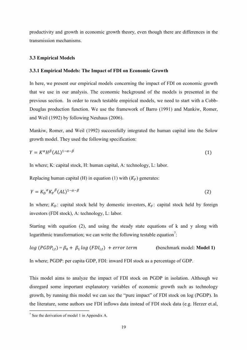
3.3 Empirical Models

3.3.1 Empirical Models: The Impact of FDI on Economic Growth

In here, we present our empirical models concerning the impact of FDI on economic growth

that we use in our analysis. The economic background of the models is presented in the

previous section. In order to reach testable empirical models, we need to start with a Cobb-

Douglas production function. We use the framework of Barro (1991) and Mankiw, Romer,

and Weil (1992) by following Neuhaus (2006).

Mankiw, Romer, and Weil (1992) successfully integrated the human capital into the Solow

growth model. They used the following specification:

� = ����(��)�� (1)

In where; K: capital stock, H: human capital, A: technology, L: labor.

Replacing human capital (H) in equation (1) with (��) generates:

� = ������(��)�� (2)

In where; �� : capital stock held by domestic investors, �� : capital stock held by foreign

investors (FDI stock), A: technology, L: labor.

Starting with equation (2), and using the steady state equations of k and y along with

logarithmic transformation; we can write the following testable equation7:

��� (�� �!,#) = $% + $ ��� (& '!,#) + ())�) *()+ (benchmark model: Model 1)

In where; PGDP: per capita GDP, FDI: inward FDI stock as a percentage of GDP.

This model aims to analyze the impact of FDI stock on PGDP in isolation. Although we

disregard some important explanatory variables of economic growth such as technology

growth, by running this model we can see the “pure impact” of FDI stock on log (PGDP). In

the literature, some authors use FDI inflows data instead of FDI stock data (e.g. Herzer et.al, 7 See the derivation of model 1 in Appendix A.

20

2008; Johnson, 2006) as a proxy of the rate of FDI stock (,�). However, Neuhaus (2006,

p.98) mentions that “the ratio of FDI stock to GDP is more accurate than the FDI flows in

capturing the sustaining effect of FDI on economic growth”. For this reason, we follow

Neuhaus (2006) and Olofsdotter (1998) and use the data of “inward FDI stock as a percentage

of GDP” instead of “inward FDI inflows as a percentage of GDP” in our models. In some

studies, authors do not choose taking the log values of percentage variables that they can get

semi-elasticities by estimating their coefficients. But in this study, we employ double-log

(log-log) type empirical models that $ coefficients can be interpreted as the (full) elasticity

parameters of respective independent variables (Ewing &Yang, 2009).

By estimating model 1 both for developing and developed countries, we would make a

comparison between the magnitudes of $ coefficient. We expect a positive $ coefficient for

developing and developed countries and it is more likely that the impact of FDI on economic

growth in developing countries would be higher due to two reasons. First, according to the

“convergence phenomenon” there is a negative relation between distance to world per capita

income level frontier and growth rate (Aghion & Howitt, 2009, p.158). It implies that

developing countries have more room to grow in comparison with developed countries.

Secondly, countries who are more far away from world technology frontier can achieve fast

economic growth rates and productivity gains simply by imitating technology which becomes

available to them via FDI and international trade.

Nonetheless, the expected positive impacts of FDI on economic growth rates in developing

and developed countries are closely dependent on some factors. Absorption capacity is the

first factor that is widely discussed and used in similar empirical FDI studies (e.g. Johnson,

2006). Several proxies are used by authors to model absorption capacity of a country. In the

literature, the most common proxy for absorption is the “schooling or educational attainment

rates” by following Barro (1991). Fortunately, we have found another absorption capacity

proxy namely “labor quality” which is developed by Bonthuis (2010). Labor quality index is a

more complete proxy then schooling data since it takes differences among schooling

indicators across countries. To reflect the role of absorption capacity we add “labor quality”

as an independent variable into model 1 and reach model 2. In model 2, we expect a

positive $- coefficient in developing and developed countries. Unlike FDI impact, we cannot

predict the relative magnitude of $- in developing and developed countries since absorption

(labor quality) is critically important in assessing the impacts of FDI in all countries. It is

21

expected that as countries raise their labor quality indices, they can both attract more FDI and

reach high growth rates. Additionally, “learning by doing” process takes place in a faster way

among high quality workers which reduces the installation costs and time for adaptation of

new investments which held by foreign investors.

��� (�� �!,#) = $% + $ ��� (& '!,#) + $- ��� (�.!,#) + ())�) *()+ (Model 2)

The second important factor that we consider in our analysis is “openness”. Together with

absorption, it is commonly used as an additional explanatory variable in FDI-led growth

studies (e.g. Neuhaus, 2006). According to international trade theory, more open economies

tend to grow faster which is supported by several empirical studies such as (Soysa &

Neumayer, 2005; Frankel & Romer, 1999).

With regard to FDI, openness has a special importance. First of all, more open economies can

attract more FDI.8 The case of China is a good example of this. As China has started to open

its economy to the world markets then it has become the leading country in terms of volumes

of total FDI inflows. Not only China experienced FDI surge for several years but also enjoyed

high and sustained economic growth rates while its openness is rising. In this regard, in model

3 we expect a positive $/ coefficient that implies openness triggers economic growth.

However, the magnitudes of the $/ coefficient may differ across the samples of developing

and developed countries due to the different degrees of openness.

��� (�� �!,#) = $% + $ ��� (& '!,#) + $- ��� (�.!,#) + $/ ��� (0�12!,#) + ())�) *()+

(Model 3)

The last factor that we consider as an additional independent variable in our analysis is the

annual inflation rate. In the literature, it is discussed that high inflation implies price

instability which decreases FDI attractiveness of the country (Neuhaus, 2006). Strictly

speaking, high inflation distorts the macroeconomic stability, expectations, and investment

decisions of domestic and foreign investors in a country (Fischer, 1993; Bleaney, 1996).

Gokal and Hanif (2004, p.11) summarize this: “through its impact on capital accumulation,

investment and exports, inflation can adversely impact a country’s growth rate”. Furthermore,

there is strong empirical evidence that inflation is detrimental to growth and capital

8 See Figure 2 in Appendix B, which demonstrates the positive association between openness and FDI.

22

accumulation (e.g. Briault, 1995; Bleaney, 1996). In our FDI-growth context, we use annual

inflation rate as an independent variable to model macroeconomic instability by following

Ismihan et. al (2002). We use the logarithms of the inflation rate variable to obtain

consistency with other variables and also to be able to interpret $3 coefficient as the full

elasticity of inflation rate with respect to PGDP.9 Since it is treated as an instability factor, we

expect a negative sign for $3 coefficient in model 4. Apart from this dominant view, there are

also other views concerning the impact of inflation on growth. Tobin (1965) in his classic

article argues that higher inflation rates may raise the level of output permanently and growth

rate of output temporarily. 10 Nonetheless, according to Solow (1956) inflation is an

exogenous factor for growth that it does not have any real impact on growth (Todaro, 2000).

��� (�� �!,#) = $% + $ ��� (& '!,#) + $- ��� (�.!,#) + $3 ��� ('2&!,#) + ())�) *()+

(Model 4)

With model 4, we conclude the presentation of our models which aim to analyze the impact of

FDI and some other additional variables on log (PGDP). In other words, estimation of models

1 to 4 would put forward the impact of FDI on economic growth which encapsulates both

“capital widening and deepening impacts”. To sum up, by estimating models 1 to 4 we aim to

reveal:

• Whether FDI is an important factor for economic growth (capital deepening + capital

widening impacts).

• To what extent the impact of FDI on economic growth alters between the samples of

developing and developed countries.

• Whether the additional independent variables have expected signs and the possible

implications of these results.

• To what extent the impact of FDI on economic growth alters across models which can

be seen as an informal way of checking the robustness of $ coefficient.

9 The standard deviation of inflation rate can also be used instead of raw inflation data (e.g. Neuhaus, 2006) but

we follow Ismihan et. al (2002) and use raw inflation data on consistency grounds. 10 See Gokal and Hanif (2004) for an extensive review of the impact of inflation on growth.

23

3.3.2 Empirical Models: The Impact of FDI on Productivity

After having completed the presentation of empirical models concerning the impact of FDI on

economic growth, in this section we go further and present four additional models in which

the dependent variables are productivity measures instead of PGDP. The theoretical

background of these models is discussed in section 3.2.2 where capital deepening impact is

explained.

In models 5 and 6, we use “labor productivity” as the dependent variable and employ FDI and

labor quality (absorption capacity) as the independent ones.11 In models 7 and 8, we employ

“total factor productivity” as the dependent variable instead of labor productivity and use FDI

and labor quality (absorption capacity) as the independent variables.

��� (��!,#) = $% + $ ��� (& '!,#) + ())�) *()+ (Model 5)

��� (��!,#) = $% + $ ��� (& '!,#) + $- ��� (�.!,#) + ())�) *()+ (Model 6)

��� (4&�!,#) = $% + $ ��� (& '!,#) + ())�) *()+ (Model 7)

��� (4&�!,#) = $% + $ ��� (& '!,#) + $- ��� (�.!,#) + ())�) *()+ (Model 8)

By estimating these additional four models both for the samples of developing and developed

countries, we aim to analyze:

• Whether FDI is an important factor for productivity (capital deepening impact).

• Whether the impact of FDI on productivity differs significantly between the samples

of developing and developed countries.

• Whether the labor quality (absorption capacity) matters for productivity.

• Whether the use of labor productivity or total factor productivity measures might

affect the results.

A final remark on our model set-up is concerning the interaction terms. As you see, in our

models we do not employ the interaction terms of FDI with other independent variables.

Because the use of interaction terms distorts our estimation results remarkably moreover they

are estimated as insignificant probably due to the multicollinearity problem. In a similar

11 It is worth noting that in models 5-8, we do not consider openness and inflation as additional independent

variables to concentrate on the impacts of FDI and labor quality on productivity.

24

study, Olofsdotter (1998) faced with the same problem that she could find only one of the

interaction term out of four to be significant at 10 percent level. She explains these

insignificant interaction terms with multicollinearity problem (high correlation among

independent variables) which stems from the use of independent variables and their

interaction terms simultaneously (Olofsdotter, 1998, p.541; Ewing &Yang, 2009).

We close this section with Tables 2 and 3 in which we present the explanations of the

variables and expected signs of the coefficients of the respective independent variables.12

Table 2: Definitions of the Dependent and Independent Variables

Table 3: Expected Signs of the Coefficients of Independent Variables

12 Technical details and calculation of the datasets are explained in section 4.

PGDP : Real per capita gross domestic product (per capita income)

FDI : Value of inward stock of foreign direct investment in country i as a percentage of GDP

LQ : The level of labor quality index

OPE* : The level of openness index, calculated as (EX+IMP) / GDP

I*F : Inflation rate based on consumer price index

LP : The level of labor productivity

TFP : The level of total factor productivity

log (FDI) log (LQ) log (OPE*) log (I*F)

Model 1 log (PGDP) +

Model 2 log (PGDP) + +

Model 3 log (PGDP) + + +

Model 4 log (PGDP) + + + -

Model 5 log (LP) +

Model 6 log (LP) + +

Model 7 log (TFP) +

Model 8 log (TFP) + +

Independent Variables

Model *o Dependent Variable

25

4. DATA

In this section, we first present the sources and description of datasets. Then, in section 4.2 we

define our sample groups.

4.1 Sources and Description of Data

To analyze the impacts of FDI on productivity and economic growth, we have developed

eight models in the previous section. In these models, totally we use different seven variables.

Below we explain briefly how we gathered and constructed the datasets of each variable in

turn.

Real per capita GDP data are gathered from The Conference Board-Total Economy database

which are in 1990 US$ (converted at Geary Khamis PPPs). After collecting the real per capita

GDP level data, we converted level data into the logarithmic form and gathered PGDP

variable to use in our estimations as Mankiw et.al (1992), and Herzer et.al (2008) did.

We collected the data of “inward FDI stock as a percentage of GDP” data for “FDI” variable

from UNCTAD-FDI database.13 It is important to note that we do not use the level data of the

“value of FDI stock” since it is only available at current prices at the database and for 20

countries it is difficult to construct a common deflator to convert current measures into real

terms. After collecting the data of “inward FDI stock as a percentage of GDP”, we took the

logarithms of the series to use in our estimations, as Ewing & Yang (2009) did.

We collected the data for “labor quality” from The Conference Board-Total Economy

Database. Originally, labor quality index is constructed by Bonthuis (2010) which uses

educational attainment as the key variable for labor quality with attaining special importance

to cross-country differences. He constructs his labor quality index by employing three

different datasets regarding educational attainment to reduce cross-country differences in

measurement of educational attainment data. In this respect, we believe that his labor quality

index is a more complete “absorption capacity” measure than a raw “schooling” data. At the

Conference Board-Total Economy Database, labor quality data are available in growth rates

13 “FDI stock is the value of the share of their capital and reserves (including retained profits) attributable to the

parent enterprise, plus the net indebtedness of affiliates to the parent enterprises” (World Investment Report,

2009).

26

form (log differences). In order to use in our estimations, first we calculated the levels of

labor quality from the growth rates by assuming an initial labor quality level value of 100.

Finally, we took the logarithms of the levels of labor quality values to use in our analysis.

Openness data are calculated by us using the IMF-IFS database. In order to calculate level of

openness index values, we gathered the data of dollar values of total Exports, Imports and

GDP (in current US$). By using the formula of (Exports + Imports)/GDP, we calculated

openness index for all 20 countries (e.g. Frankel & Romer, 1999). Finally, we took the

logarithms of the openness index values to use in our analysis.

Inflation data are derived from the IMF-IFS database. We collected the inflation data, which

is based on consumer price index, from the database and converted into logarithmic form to

use in our estimations by following Ismihan et.al (2002).

Labor productivity (output per employed person) is used as a proxy variable of economy-wide

productivity in our analysis. And data for labor productivity is derived from The Conference

Board-Total Economy Database which are in 1990 US$ (converted at Geary Khamis PPPs).

Put differently, our labor productivity level data are the level values of real output per

employed person in 1990 US$. In our analysis, the log values of the labor productivity data

are used.

The second productivity measure that we use is total factor productivity. TFP is defined as

“the portion of output not explained by the amount of inputs used in production” (Comin,

2008, p.1). In this respect, TFP is a difficult indicator to measure moreover it is not generally

available for many countries and for a long time period. 14 Fortunately, The Conference

Board-Total Economy Database presents the growth rates of TFP for different countries and

for a sufficient length of time, which is estimated as Tornqvist index.15 However, to use in our

estimations we need log values of level TFP data. Therefore, first we calculated the levels of

TFP from the growth rates of TFP by assuming an initial TFP level value of 100. Then, we

converted these calculated level TFP values into logarithms to use in our analysis.

14 See the discussion in Tica and Druzic (2006, p.11) and Lee (2009) on this issue. 15“Tornqvist index allows both quantities purchased of the inputs to vary and the weights used in summing the

inputs to vary, reflecting the relative price changes.” (Bureau of Labor Statistics, 2010).

27

Table 4: Summary of Data Sources and Description

4.2 Definition of Samples

We collected and constructed our dataset over the period 1984-2008 and for two different

sample groups namely “developing” and “developed” countries. Each sample group consists

of 10 countries. In our panel dataset, T is 25 years and N is 20 countries. Thus, we have

totally (20*25) 500 observations for each series. In this study, totally we employ seven

different series hence number of total observations equals (500*7) 3500.

We chose our sample countries according to their classifications in UNDP Human

Development Report, 2009. In this report, countries are classified in four main different

categories namely; “very high human development (developed countries)”, “medium human

development (developing countries)”, “high human development (developing countries)”, and

“low human development (least developed countries)” according to their development

indices.

Variables Gathered from Databases Data Source Data Conversion Logarithmic Form

of Level Values

Real per capita GDP(in 1990 US$ at Geary Khamis PPPs)

The Conference Board Total Economy Database

No log (PGDP)

FDI stock as a percentage of GDP UNCTAD-FDI Database No log (FDI)Growth of Labor Quality Index The Conference Board

Total Economy DatabaseLevels are calculated

from growth rates

log (PGDP)

Openness index IMF-IFS Database(calculated by us)

No log (OPEN)

Inflation(Consumer price index is used)

IMF-IFS Database No log (INF)

Labor productivity (output per person employed)

(in 1990 US$ at Geary Khamis PPPs)

The Conference Board Total Economy Database

No log (LP)

Total Factor Productivity Growth (Estimated as Tornqvist index)

The Conference Board Total Economy Database

Levels are calculated

from growth rates

log (TFP)

28

Table 5: Sample Groups

In our developing countries sample, there are 5 medium human development category (China,

Egypt, India, South Africa, Thailand) and 5 high human development category (Brazil,

Colombia, Mexico, Turkey, Uruguay) countries. Our developed countries sample contains 5

relatively large (France, Italy, Japan, UK, USA) and 5 relatively small countries (Austria,

Denmark, Netherlands, Sweden, Switzerland) in terms of their amount of total GDP. By

adding different types of counties into the sample groups, we aim to increase the homogeneity

within sample groups which help us in reducing sample selection bias. Nonetheless, one may

argue that 10-country might not be sufficient to reduce the sample selection bias. But the data

limitation has enforced us to work totally with 20 countries for 25-year period in this study.

Last but not least, we use annual data in our estimations. In some empirical studies (e.g.

Ewing & Yang, 2009; Neuhaus, 2006), authors choose using 5-year averages to reduce the

impact of business cycles to the coefficients of the regression models. In fact, the use of

annual or 5-year averages did not alter our estimation results remarkably (see Table 6 in

Appendix B). Therefore, we have always used data in annual form throughout this study. 16

5. METHODS A*D ESTIMATIO* RESULTS

In this section, we first describe the methods that we use in the analysis. Then, we present and

discuss the results of the tests and estimations in sections 5.2, 5.3, and 5.4.

16 See Olofsdotter (1998), Herzer et.al (2008), and Lee (2009) for studies which use annual data.

G1 G2

(Developing countries) (Developed Countries)

1. Brazil 1. Austria

2. China 2. Denmark

3. Colombia 3. France4. Egypt 4. Italy

5. India 5. Japan

6. Mexico 6. Netherlands7. South Africa 7. Sweden

8. Thailand 8. Switzerland

9. Turkey 9. UK10. Uruguay 10. USA

29

5.1 Methods

As mentioned in introduction, one of the distinguishing features of the study is its use of both

panel cointegration and panel estimation methods in analyzing the impacts of FDI on

productivity and economic growth in developing and developed countries. We carry out the

analysis in four steps and Table 7 summarizes the tests and methods that we employ

throughout the analysis.

Steps of the Analysis:

• First, we conduct panel unit root tests for our seven series. In order to be able to search

for panel cointegration among series, they should have the same order of integration.

Therefore, we first need to carry out panel unit root tests.

• Second, we conduct panel cointegration tests among the variables that we use in eight

different models. By doing this, we analyze whether there are long-run relations

among variables in our models.

• Third, we run eight models by using panel OLS method to estimate the coefficients of

the variables. The panel cointegration analysis only provides qualitative evidence

whereas the estimation of the coefficients would provide quantitative evidence.

Therefore, we can make comparisons regarding the sizes and significance of the

coefficients across models and samples.

• Finally, we interpret the estimation results in section 5.4.

Table 7: Employed Tests and Methods

5.2 Panel Unit Root Tests

After presenting the methodology that we follow, we start our analysis with panel unit root

tests, which is the usual way of starting cointegration analysis to identify whether the series

are stationary or non-stationary. A non-stationary series is not a mean-reverting series in

which a shock (innovation) in the series does not die away. It is formulated as “non-stationary

series have long memory” (Harris and Sollis, 2005, p.29). Therefore, linear combinations of

*ame of the Employed Tests and Methods

Test for: Panel Unit Root IPS individual unit root and Breitung common unit root testsTest for: Panel Cointegration Johansen-Fisher panel cointegration testEstimation Method Panel OLS with fixed effects

30

non-stationary series might lead to estimation of spurious regressions in which the estimated

coefficients are biased (Gujarati, 2003, p.806-807). In this regard, the identification of the

existence of non-stationarity (unit root) and its order is important in two respects:

• First, we need to know the order of unit root in the series to be able to conduct panel

cointegration tests that we can only conduct panel cointegration tests among series

which have the same order of integration. For instance, we can seek panel

cointegration in model 1, if log (PGDP) and log (FDI) are I (1).17

• Second, the order of unit root in the series is also important to get rid of spurious

regression risk when the existence of panel cointegration is not verified. In these

cases, the unit root test results are useful in converting series into the stationary form

by taking first or second differences. Otherwise, the use of non-stationary series which

are not cointegrated will lead to estimation of biased coefficients.18

Basically, in the literature of panel series there are two strands of “panel unit root tests” which

are the individual and common panel unit root tests. The IPS (Im-Peseran-Shin), Fisher ADF,

and Fisher PP tests are in the class of individual panel unit root tests whereas the Breitung,

Hadri, Levin-Li-Chu tests are the common panel unit root tests. Intuitively, the individual

panel unit root tests are less restrictive than the common panel unit root in the sense that they

allow ρ* (the coefficient of level of the series in eq.3) to vary within the panel series (Im et

al., 1997). However, in the literature it is noted that none of the panel unit root tests have an

exact superiority over another one (Verbeek, 2008, p.392-393). Put differently, there is no

common way in selecting the type of panel unit root tests to test whether there is panel unit

root. In here, to be able to eliminate the shortcomings of both types of tests, we choose to

conduct one individual panel unit (IPS) and one common unit root test (Breitung).19

The Im-Peseran-Shin (IPS) Individual Panel Unit Root Test

The IPS test estimates the value of ρ* by using the following equation in testing the existence

of unit root:

17 If a series is becoming stationary after taking the first difference, it is known as integrated of order 1 or I (1). 18 As you will see in section 5.3, we have not faced with this problem since we have found panel cointegration

among all series in the models. 19 See Baltagi & Kao (2000), Banerjee (1999), and Harris & Sollis (2005, p.191-200) for an extensive review of

panel unit root tests. See Mishra & Smyth (2010) and Apergis & Payne (2010) for some empirical examples.

31

∆7!# = 8∗7!,# + : ;!< ∆7!,#< + =!#>!<? (3)

Basically, the IPS tests the following hypotheses:

H0: ρ*=0 for all i; (All series in panel have a unit root)

H1: ρ*<0 for at least one i; (At least, one series in panel does not have a unit root)

We present the IPS test results in Table 8. By using the values in Table 8, we test unit root as

follows:

For example, according to Table 8, the level of “log (PGDP)” panel series of developing

countries is not stationary at 5% level. Because the IPS-W stat of the “level series of log

(PGDP)” is 7.02 and it is not significant at 5% level since its probability value is 1. Thus, we

accept the null hypothesis that all series in panel have a unit root. On the other hand, the “first

differences of log (PGDP)” is stationary. Because the IPS-W stat of the “first differences of

log (PGDP)” is -5.82 and it is significant at 5% level since its probability value is 0. Thus, we

accept the alternative hypothesis in this case and conclude that log (PGDP) is I (1) for

developing countries. Put differently, non-stationary series of log (PGDP) series turns to

stationary by taking the first differences thereby it is integrated of order 1. In a similar

fashion, when we conduct the IPS test for all panel series of developing and developed

countries, we reach the same conclusion that they are I (1).

The Breitung Common Panel Unit Root Test

The Breitung test uses the equation (3) as the IPS does, but it tests the following hypotheses:

H0: ρi*=0 for all i; (All series in panel have a unit root)

H1: ρi*<0 for all i; (All series in panel do not have a unit root)

We present the Breitung test results in Table 8. By using the values in Table 8, we test unit

root as follows:

For example, according to Table 8, the level of “log (PGDP)” panel series of developing

countries is not stationary at 5% level. Because the Breitung t-stat of the level series of log

(PGDP) is -1.016 and it is not significant at 5% level since its probability value is 0.15. Thus,

we accept the null hypothesis that all series in panel have a unit root. On the other hand, the

32

“first differences of log (PGDP)” series is stationary. Because the Breitung t-stat of the “first

differences of log (PGDP)” is -2.55 and it is significant at 5% level since its probability value

is 0.0053. Thus, we accept the alternative hypothesis in this case and conclude that log

(PGDP) is I (1) for developing countries. Put differently, non-stationary series of log (PGDP)

series turns to stationary by taking the first differences thereby it is integrated of order 1. In a

similar fashion, when we conduct the Breitung test for all panel series of developing and

developed countries, we reach the same conclusion that they are I (1).

All in all, there is full consistency between the findings of the IPS and Breitung tests.

Actually, it is not surprising that we have found out that all series are integrated of order one

since we use macroeconomic variables such as per capita GDP, labor productivity which tend

to be non-stationary over time. The main conclusion from panel unit root tests is that we can

search for panel cointegration among the series in our models since they all have the same

order of integration and we conduct panel cointegration tests in the next section.

5.3 Panel Cointegration Tests

When two non-stationary series are being individually nonstationary, their linear combination

can be stationary. “Economically speaking, two variables will be cointegrated if they have a

long-term, or equilibrium, relationship between them.” (Gujarati, 2003, p.822 and 830).

Basically, the Engle-Granger approach is used in existence of two individual time series. With

the contribution of Johansen (1988), multivariate cointegration analysis (cointegration in

existence of more than two time-series variables) has become available to researchers, which

has been widely used for several years.

Nonetheless, cointegration in panel series is a more complex issue than time series which

stems from the existence of cross-section units and their impacts on cointegration vectors.

Several scholars studied on panel series cointegration issue (e.g. Pedroni, 1999; Kao, 1999;

Maddala & Wu, 1999) to deal with these kinds of problems and they developed the panel

cointegration tests which are available in today’s modern econometric software programs.

Unfortunately, as mentioned by Verbeek (2008, p.392) “the drawbacks and complexities in

panel unit root tests are also relevant for the panel cointegration tests”. It implies that panel

cointegration tests still have some shortcomings such as Pedroni test reports 7 different test

33

statistics and while one of them is rejecting the null hypothesis of “no cointegration”, the

other one can accept it.

Although problems still persist, in empirical panel studies panel cointegration tests are widely

used. Because performing panel cointegration tests is the unique way of testing whether there

is a “long-run relation” among non-stationary panel series. At this stage, we put aside the

discussion on panel cointegration tests which is beyond the scope of this study, and

concentrate on the Johansen-Fisher panel cointegration test that we have conducted.20

The Johansen-Fisher Panel Cointegration Test

The Johansen-Fisher panel cointegration test is a Fisher-type test using an underlying

Johansen methodology (Maddala & Wu, 1999). The Johansen-Fisher panel cointegration test

fills an important gap in the literature that enables scholars to test whether there is a long-run

relation among panel series. Moreover, it identifies the rank of cointegration relation as the

Johansen cointegration test does in time-series datasets. In this regard, it has an advantage

over the Kao and Pedroni panel cointegration tests.

The Johansen-Fisher panel cointegration test uses two types of Fisher test statistics which are

computed from “trace and max-eigen value tests” in testing the null of “no cointegration”.

While conducting the Johansen-Fisher panel cointegration test, one should decide the

intercept and trend specification in the panel data, and the number of lags. A shortcoming of

the Johansen-Fisher panel cointegration test is that it does not suggest any systematic

approach while choosing the lag and trend specification as in the Johansen test. Nonetheless,

to make robust inferences from the Johansen-Fisher panel cointegration test results, it is

suggested to reach consistent “results” between trace and max-eigen test results. In this

respect, we have tried all five trend specification options in E-views 7 software program under

the Johansen-Fisher panel cointegration test with the smallest possible lags to get consistent

results.21

20 See the discussions in Banerjee (1999), Verbeek (2008, p.392-393), Harris & Sollis (2005, p.200-206). 21We employ “general to specific” approach which is suggested in the literature (Harris and Sollis, 2005) that we

keep the number of lags as small as possible according to Hannan-Quin lag-length selection criteria.

34

Hence, we have started to our tests with one lag and tried it under five different trend

specifications. In most of the cases, we have reached consistent results with one lag. Only in

two cases, we have used two lags for consistency purposes. Overall, we have reported the

panel cointegration test results in Tables 9 and 10 (see Appendix B) and have determined the

rank of cointegration in respective models according to these reported values.

For example, to test the existence of cointegration and determine its rank in model 1, which

includes only log (PGDP) and log (FDI) series, we follow two steps:

Step 1:

H0: r = 0 (no cointegration); H1: r ≤ 1 (at most one cointegration relation)

In Table 9, the reported Fisher stat from trace test for model 1 is 38 for developing countries

sample. It is significant at 5% level since its probability value is 0.0089. Therefore, we reject

the null and accept the alternative hypothesis. According to the reported Fisher stat from max-

eigen value test in Table 10, we reject the null and accept the alternative hypothesis as well.

Because the reported Fisher stat from max-eigen value test is 33.57 for model 1 in developing

countries sample. And it is significant at 5% level since its probability value is 0.0292. In

sum, both of the test statistics have confirmed the existence of at most one cointegration

relation.

Step 2:

H0: r ≤ 1 (at most one cointegration relation); H1: r ≤ 2 (at most two cointegration relations)

In Table 9, the Fisher stat from trace test for model 1 is 26.2. It is not significant at 5% level

since its probability value is 0.1592. Therefore, we accept the null hypothesis in this case.

According to the reported Fisher stat from max-eigen value test in Table 10, we accept the

null hypothesis as well. Because the reported Fisher stat from max-eigen value test is 26.2 for

model 1 in developing countries sample. And it is not significant at 5% level since its

probability value is 0.1592. In conclusion, according to the both trace stats and max-eigen

values under the Johansen-Fisher panel cointegration test; we have determined that there is

panel cointegration relation between “log (PGDP) and log (FDI) series”, and the rank of the

cointegration relation is 1.

In a similar fashion, when we repeat the similar steps for our eight models for developing and

developed country samples, we confirm the existence of cointegration in all cases. And in our

35

test results it is found out that the rank of cointegration lies between 1 and 4. 22 Put

differently, we have found long-run relations among all variables that we use in our models.

By finding cointegration relations among the series that we use in our models, the estimation

of spurious regression risk has been eliminated.

5.4 Estimation Method and Results

5.4.1 Estimation Method

After finding the existence of long-run relations among the panel series, now we need to

estimate the size and sign of these relations. In other words, cointegration analysis has only

verified the existence of long-run relations among the variables of eight models. But we need

quantitative values to be able to make interpretations and comparisons. We do this by

estimating our models, in which variables are cointegrated, by using panel OLS method

allowing for fixed effects and along with White heteroscedasticity consistent standard

errors.23

In panel estimation literature, panel OLS (fixed effect estimator) and dynamic OLS methods

are in the class of parametric approaches whereas FM (fully modified) OLS is a non-

parametric approach. Nonetheless, as in panel unit root and cointegration tests, there is no

consensus among scholars which estimation method performs better in estimating less-biased

and more robust coefficients. For example, Kao and Chiang (2000) showed that FMOLS may

be more biased than DOLS” (Harris and Sollis, 2005, p.207). But Banerjee (1999) claims

FMOLS or DOLS are asymptotically equivalent for more than 60 observations.24 Apart from

these approaches, in some panel studies, authors prefer estimating the coefficients of the

cross-section units separately by using OLS and calculate the mean coefficients for the whole

panel by taking the simple average of the estimated coefficients of cross-section units. This

method is known as mean group estimation. Bearing the discussion above in mind, we

employ panel OLS method because:

• Many scholars are skeptic about the use of either recently developed FMOLS or

DOLS method. Because none of them has distinct superiority over the other method.

22 For model 4, the trace test finds the rank of cointegration as 3, but max-eigen test finds it as 4. Additionally,

we have also verified the existence of cointegration by Kao panel cointegration test among the series of model 4. 23 See Olofsdotter (1998) and Ewing & Yang (2009) for studies which use panel OLS method. 24 See Harris and Sollis (2005, p.207) for discussion.

36

• Panel OLS method is the most common estimation technique which is available in

almost all econometric software programs. With panel OLS method, researchers can

easily estimate their equations with taking fixed or random effects, and

heteroscedasticity-consistent standard errors into consideration. Nonetheless, in many

software programs, researchers should write their own code to estimate a panel

regression with DOLS or FMOLS method which sometimes lead inconsistent

results.25

• Finally, the use of DOLS method requires inclusion of lags into the models. Since we

use more than one independent variables, it might lead further econometric problems

(e.g. multicollinearity, endogeneity). Therefore, we choose to employ panel OLS

method in this study.

Panel OLS Method

After this quick overview on panel estimation methods, we briefly explain panel OLS

estimation method-with fixed effects. The panel OLS method, is the application the of the

usual OLS method to the panel series. A panel series dataset has both time-unit dimension (T)

and cross-unit dimension (N). Thus, neither cross-section nor time-series estimators of OLS

method can generate unbiased results. In this respect, panel OLS estimators take both time

and cross-section units into consideration in estimation process. However, there can be cross-

country differences within time-series which can lead endogeneity problem (Aghion &

Howitt, 2009, p.452). Hence, estimation results without taking cross-country differences into

consideration might lead misinferences about coefficients. To deal with this problem, “the

fixed effect estimators of panel OLS is developed, which captures the omitted variables that

are present in each country and that are constant over time” (Aghion & Howitt, 2009, p.453).

Basically, the fixed effect can be applied by constructing a dummy variable for each cross-

section unit (country) which does not change over time. Fortunately, in E-views software

program this can be done automatically by selecting cross-section fixed-effects from panel

options while estimating the regressions that we do not need to construct these dummy

variables separately.

Another factor that can lead misinferences by leading biases in standard errors of the

coefficients is heteroscedasticity problem in use of panel series. To eliminate this possibility 25 For example, E-views 7 software program, which is developed in 2009, still does not allow FMOLS method in

estimation of panel series.

37

we choose White cross-section heteroscedasticity consistent co-variance method in E-views

software while running our regressions, which is a standard procedure in panel estimations

(see Olofsdotter, 1998).

To sum up econometric issues concerning the estimation of our models:

• We have eliminated spurious regression risk in existence of non-stationary series,

which might lead biased estimators, by searching and finding cointegration relations

among the variables of all models.

• The cross-country differences which do not change over time might lead endogeneity

problem. And this possibility is eliminated by allowing for fixed effects in estimations

of the models.

• The possibility of biased standard errors which might lead to make misinferences

about estimated coefficients is eliminated by choosing White’s cross-section

heteroscedasticity consistent co-variance method in estimations of the models.

5.4.2 Estimation Results

By using the framework described above, we run our models and present the estimation

results in Tables 11, 12, and 13.

5.4.2.1 Estimation Results: The Impact of FDI on Economic Growth

Table 11: Estimation Results of Models 1 to 4

*otes: (1) Values without parentheses are estimated coefficients. (2) Bold numbers denote that they are

significant at 5 % significance level. (3) Probabilities of t-statistics are in parentheses. (4) G1: Developing

countries sample and G2: Developed countries sample.

Dependent: log (PGDP)

G1 G2 G1 G2 G1 G2 G1 G2

Intercept 7.7563

(0.0000)

9.4765

(0.0000)

-2.6096

(0.0006)

-0.4360

(0.0071)

-2.0910

(0.0002)

-0.4289

(0.0005)

-2.6984

(0.0000)

-0.5435

(0.0097)

log (FDI) 0.2554

(0.0000)

0.1718

(0.0000)

0.1543

(0.0000)

0.0680

(0.0000)

0.0836

(0.0002)

0.0688

(0.0000)

0.0870

(0.0001)

0.0810

(0.0000)

log (LQ) 2.2681

(0.0000)

2.1794

(0.0000)

2.2403

(0.0000)

2.1768

(0.0000)

2.3623

(0.0000)

2.1886

(0.0000)

log (OPE*) 0.1998

(0.0006)

-0.0038

(0.9337)

0.1968

(0.0006)

-0.0258

(0.5550)

log (I*F) 0.0129

(0.1013)

0.0127

(0.0727)

Adjusted R-sq 0.8901 0.857 0.9136 0.8983 0.9204 0.8979 0.9205 0.9083

Model 1 Model 2 Model 3 Model 4

38

Table 11 documents the estimation results of models 1 to 4 in which the dependent variable is

log (PGDP).26 According to estimation results for the samples of developing and developed

countries:

• In model 1 (the benchmark model), the coefficient of log (FDI) is estimated as positive

and significant, as expected. It is 0.25 for developing and 0.17 for developed countries.

And in both samples the coefficients of log (FDI) are significant at 5% level. Thus, 1

percent rise in “FDI stock/GDP ratio” increases economic growth 0.25 percent in

developing and 0.17 percent in developed countries.27 The findings are also consistent

with the prediction of the convergence phenomenon of economic growth theory. Since

developing countries are more far away from the “world average per capita income” that

they can reach fast growth rates simply by transferring foreign capital (capital widening

impact) and imitating the technology which is improved by developed countries (capital

deepening impact). In addition, model 1 has a high goodness of fit (R-square) that 89 and

85 percent of the variation in log (PGDP) can be explained by log (FDI) in developing and

developed countries respectively.28

• In model 2, our interest variable is labor quality. According to estimation results, the

coefficient of log (LQ) is estimated as positive and significant at 5% level which is 2.26

for developing and 2.17 for developed countries. Therefore, 1 percent rise in labor quality

increases economic growth 2.26 percent in developing and 2.17 percent in developed

countries. Model 2 has high explanatory power for both of the samples. Unlike the

coefficient of log (FDI), we do not see a considerable difference in the magnitudes of the

coefficient of log (LQ) across developing and developed countries. This implies that labor

quality is an important factor for absorption in both developing and developed countries.29

Put differently, as countries raise the quality of labor by increasing the number of

schooling years and quality of education, they can experience high growth rates since their

absorption capacities increase in accordance with labor quality. Moreover, these countries

26 In our interpretations of the estimation results, we do not make comments on the intercept terms since they do

not have any economic importance in our model set-up. 27 Our estimation results are in line with the findings of several authors such as Neuhaus (2006), Olofsdotter

(1998) in terms of positive and significant growth impact of FDI. 28 High R-square values do not only stem from high explanatory power of the models but also stem from the use

of panel series. 29 See a similar conclusion in Johnson (2006) and Ewing & Yang (2009).

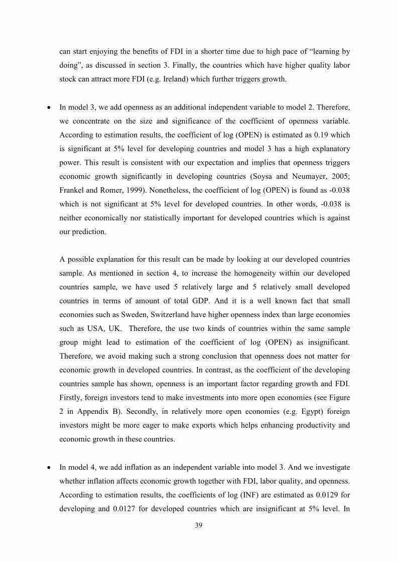
39

can start enjoying the benefits of FDI in a shorter time due to high pace of “learning by

doing”, as discussed in section 3. Finally, the countries which have higher quality labor

stock can attract more FDI (e.g. Ireland) which further triggers growth.

• In model 3, we add openness as an additional independent variable to model 2. Therefore,

we concentrate on the size and significance of the coefficient of openness variable.

According to estimation results, the coefficient of log (OPEN) is estimated as 0.19 which

is significant at 5% level for developing countries and model 3 has a high explanatory

power. This result is consistent with our expectation and implies that openness triggers

economic growth significantly in developing countries (Soysa and Neumayer, 2005;

Frankel and Romer, 1999). Nonetheless, the coefficient of log (OPEN) is found as -0.038

which is not significant at 5% level for developed countries. In other words, -0.038 is

neither economically nor statistically important for developed countries which is against

our prediction.

A possible explanation for this result can be made by looking at our developed countries

sample. As mentioned in section 4, to increase the homogeneity within our developed

countries sample, we have used 5 relatively large and 5 relatively small developed

countries in terms of amount of total GDP. And it is a well known fact that small

economies such as Sweden, Switzerland have higher openness index than large economies

such as USA, UK. Therefore, the use two kinds of countries within the same sample

group might lead to estimation of the coefficient of log (OPEN) as insignificant.

Therefore, we avoid making such a strong conclusion that openness does not matter for

economic growth in developed countries. In contrast, as the coefficient of the developing

countries sample has shown, openness is an important factor regarding growth and FDI.

Firstly, foreign investors tend to make investments into more open economies (see Figure

2 in Appendix B). Secondly, in relatively more open economies (e.g. Egypt) foreign

investors might be more eager to make exports which helps enhancing productivity and

economic growth in these countries.

• In model 4, we add inflation as an independent variable into model 3. And we investigate

whether inflation affects economic growth together with FDI, labor quality, and openness.

According to estimation results, the coefficients of log (INF) are estimated as 0.0129 for

developing and 0.0127 for developed countries which are insignificant at 5% level. In

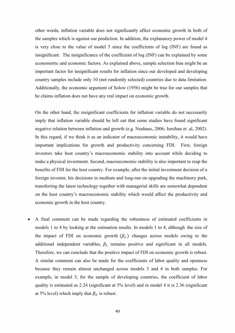
40

other words, inflation variable does not significantly affect economic growth in both of

the samples which is against our prediction. In addition, the explanatory power of model 4

is very close to the value of model 3 since the coefficients of log (INF) are found as

insignificant. The insignificance of the coefficient of log (INF) can be explained by some

econometric and economic factors. As explained above, sample selection bias might be an

important factor for insignificant results for inflation since our developed and developing

country samples include only 10 (not randomly selected) countries due to data limitation.

Additionally, the economic argument of Solow (1956) might be true for our samples that

he claims inflation does not have any real impact on economic growth.

On the other hand, the insignificant coefficients for inflation variable do not necessarily

imply that inflation variable should be left out that some studies have found significant

negative relation between inflation and growth (e.g. Neuhaus, 2006; Ismihan et .al, 2002).

In this regard, if we think it as an indicator of macroeconomic instability, it would have

important implications for growth and productivity concerning FDI. First, foreign

investors take host country’s macroeconomic stability into account while deciding to

make a physical investment. Second, macroeconomic stability is also important to reap the

benefits of FDI for the host country. For example, after the initial investment decision of a

foreign investor, his decisions in medium and long-run on upgrading the machinery park,

transferring the latest technology together with managerial skills are somewhat dependent

on the host country’s macroeconomic stability which would affect the productivity and

economic growth in the host country.

• A final comment can be made regarding the robustness of estimated coefficients in

models 1 to 4 by looking at the estimation results. In models 1 to 4, although the size of

the impact of FDI on economic growth ($ ) changes across models owing to the

additional independent variables, $ remains positive and significant in all models.

Therefore, we can conclude that the positive impact of FDI on economic growth is robust.

A similar comment can also be made for the coefficients of labor quality and openness

because they remain almost unchanged across models 3 and 4 in both samples. For

example, in model 3, for the sample of developing countries, the coefficient of labor

quality is estimated as 2.24 (significant at 5% level) and in model 4 it is 2.36 (significant

at 5% level) which imply that $- is robust.

41

5.4.2.2 Estimation Results: The Impact of FDI on Productivity

Table 12: Estimation Results of Models 5 and 6

*otes: (1) Values without parentheses are estimated coefficients. (2) Bold numbers denote that they are

significant at 5 % significance level. (3) Probabilities of t-statistics are in parentheses. (4) G1: Developing

countries sample and G2: Developed countries sample.

Table 12 documents the estimation results of models 5 and 6 in which the dependent variable

is log (LP). According to estimation results for the samples of developing and developed

countries:

• In model 5, the coefficients of log (FDI) are estimated as positive and significant, as

expected for both samples. It is 0.21 for developing and 0.14 for developed countries

which are significant at 5% level. Thus, 1 percent rise in “FDI stock/GDP ratio” increases

labor productivity 0.21 percent in developing and 0.14 percent in developed countries.

This finding is also consistent with the prediction of economic growth theory and the

convergence phenomenon. Although developing countries carry out relatively less

research and developed activities, they have a higher coefficient for log (FDI) variable, as

in model 1. Because they have more room to imitate the technology transferred via FDI.

Additionally, developing countries might not only imitate the transferred technology

legally but also they might do this illegally due to the existence of weak property-rights in

these countries. Hence, FDI might trigger labor productivity in developing countries to a

higher extent. Briefly, positive and significant coefficients for log (FDI) variable for the

samples of developing and developed countries imply that “capital deepening” takes place

as FDI stocks increase. Finally, model 5 and 6 have high goodness of fit (R-square)

which are 0.90 and 0.89 in developing and developed countries, respectively.

• In model 6, we add labor quality variable to model 5. According to estimation results, the

coefficients of log (LQ) are estimated as positive and significant at 5% level which is 1.74

Dependent: log (LP)

G1 G2 G1 G2

Intercept 8.7979

(0.0000)

10.2890

(0.0000)

0.8164

(0.0023)

3.1523

(0.0000)

log (FDI) 0.2165

(0.0000)

0.1479

(0.0000)

0.1386

(0.0000)

0.0731

(0.0000)

log (LQ) 1.7464

(0.0000)

1.5693

(0.0000)

Adjusted R-sq 0.9063 0.8927 0.9176 0.9191

Model 5 Model 6

42

for developing and 1.56 for developed countries. The findings are also in line with the

estimation results of model 2 that improvements in labor quality enhance labor

productivity. Put differently, labor quality does not only important for economic growth

but also for productivity. Thus, the importance of absorption capacity variable has been

verified in both samples of developing and developed countries.

Table 13: Estimation Results of Models 7 and 8

*otes: (1) Values without parentheses are estimated coefficients. (2) Bold numbers denote that they are

significant at 5 % significance level. (3) Probabilities of t-statistics are in parentheses. (4) G1: Developing

countries sample and G2: Developed countries sample.

Table 13 documents the estimation results of models 7 and 8 in which the dependent variable

is log (TFP). According to estimation results for the samples of developing and developed

countries:

• In model 7, the coefficient of log (FDI) is estimated as 0.0071 but insignificant at 5%

level for the sample of developing countries, which is against our prediction. On the other

hand, it is estimated as 0.0365 for the sample of developed countries which is significant

at 5% level. Thus, 1 percent rise in “FDI stock/GDP ratio” increases total factor

productivity by 0.03 percent in developed countries. Hence, one can conclude that log

(FDI) does not significantly enhance total factor productivity in developing countries but

weakly in developed countries. Such a conclusion might be explained by several

econometric and economic factors:

a) Sample-selection bias and country-heterogeneity in the sample of developing

countries might lead insignificant result for the coefficient log (FDI) in model 7.

b) Miscalculation of TFP data might also lead insignificant result for the coefficient

log (FDI) in model 7. As it is known, calculation of TFP requires both data of

“capital and labor stock” of a country. On the other hand, poor data quality

Dependent: log (TFP)

G1 G2 G1 G2

Intercept 4.5101

(0.0000)

4.6069

(0.0000)

3.3791

(0.0173)

1.6031

(0.0008)

log (FDI) 0.0071

(0.3946)

0.0365

(0.0000)

-0.0290

(0.0959)

0.0050

(0.3682)

log (LQ) 0.2599

(0.3864)

0.6604

(0.0000)

Adjusted R-sq 0.7598 0.8092 0.7673 0.8285

Model 7 Model 8

43

problem is a well-known fact especially for developing countries. Therefore, poor

data quality, which lead miscalculation of TFP, might be an explanation for

insignificant result in developing countries. (Sargent & Rodriguez, 2000, p.43).

c) We also need to consider other studies findings regarding the impact of FDI on

productivity in developing countries. Several authors have found out that

productivity impact of FDI is not significant in China and India (e.g. Sjöholm,

2008; Buckley et.al, 2006; Sasidharan, 2006). In this regard, for our developing

countries sample, the insignificant coefficient for log (FDI) might be a correct

estimation. But then, this result seems not to be consistent with the estimation

result of model 5. Because in model 5, we have concluded above that FDI triggers

“labor productivity” in developing countries sample. This inconsistency brings us

to a well-known discussion in economics about the use of best productivity

measure. We refer discussion to the literature and conclude that FDI weakly

triggers TFP in developed countries but not in developing countries.30

• In model 8, we add labor quality to model 7. Thus, our interest variable is labor quality.

According to estimation results, the coefficient of log (LQ) is estimated as 0.25 but it is

insignificant at 5% level for developing countries. However, for developed countries it is

found as 0.66 and significant at 5% level, as expected. Additionally, in model 8, the

coefficient of log (FDI) is estimated as insignificant at 5% in both samples.

Aforementioned, poor TFP data quality discussion for developing countries might be also

applied to here in explaining positive but insignificant coefficient of log (LQ). Because, in

all other models we have always found that labor quality enhances productivity and

economic growth in developing countries.

6. CO*CLUSIO*S A*D IMPLICATIO*S

In this final section, we gather the major findings of panel cointegration analysis and

estimation results and interpret them without technical details. Moreover, we discuss the

possible implications of these major findings and conclude the study.

30 See the discussion in Sargent & Rodriguez (2000). According to them, TFP seems to be a better productivity

measure but there are also proponents of LP therefore there is no clear conclusion in the discussion.

44

The study’s major findings reveal that:

• There is a long-run relation between “log (PGDP) and log (FDI)” variables. And the

coefficient of the long-run relation is estimated as positive and significant for both

samples in model 1. In other words, it is verified that FDI triggers economic growth in

developing and developed countries. Besides, the impact of FDI on economic growth

is found in developing countries relatively higher than developed countries which can

be explained by the convergence phenomenon.

• Although long-run relation is found between “log (LP) and log (FDI)”, and “log (TFP)

and log (FDI)” variables, the positive impact of FDI on productivity is only partly

verified. By using labor productivity as the dependent variable, we conclude FDI

enhances productivity in both developing and developed countries. But when we use

total factor productivity as the dependent variable, the positive and statistically

significant impact of FDI on productivity is only found for “developed countries

sample” in model 7.

• The magnitudes of productivity impacts of FDI are smaller than the magnitudes of

growth impacts of FDI in estimations. Because the magnitudes of growth impact ($ in model 1) reflect both capital widening and deepening effects whereas the

magnitudes of productivity impact ( $ in model 5 and 7) reflect only capital

deepening effect. Put differently, the productivity impact of FDI is limited in

comparison with growth impact of FDI, as expected. It is also consistent with the

prediction of the endogenous growth models in which the research and development

activities conducted within the country are the key element for technology

(productivity) growth rather than other factors such as FDI, international trade

(Aghion & Howitt, 2009).

• The impacts of a number of additional independent variables have been investigated in

the study. First of all, in all models the existence of long-run relations among variables

is verified by cointegration tests. Secondly, the labor quality (absorption capacity) is

found as a significant factor in promoting growth and productivity in both developing

and developed countries. Thirdly, it is showed that more open developing economies

tend to grow faster that the coefficient of openness is estimated as positive and

significant. Finally, the impact of inflation on growth could not be verified due to

insignificant coefficients for inflation variable in both developing and developed

countries.

45

The possible implications of these major findings can be summarized as follows:

• The major implication of the finding “FDI triggers economic growth” is that; both

developing and developing countries need to pursue pro-FDI policies to attract more

FDI which will boost their economic growth. Nonetheless, as discussed in section 3,

the size of the growth impact can alter regarding the type of FDI (greenfield versus

brownfield; vertical versus horizontal FDI). In this respect, pro-FDI policies should

not only designed for attracting high volumes of FDI but also right kinds of FDI to

induce economic growth to a higher extent. For example, governments can promote

investments of foreigners into some selected or prioritized sectors (e.g. IT, R&D) for

long-run growth and development. A successful example of pro-FDI policies with a

long-run development perspective is followed by Ireland. Önis and Senses (2007)

summarize this issue very well: “States try to adopt pro-active policies through various

direct and indirect mechanisms to upgrade the performance of national firms as well

as attracting in competition with other states the right kinds of FDI needed for long-

term transformation. As the experience of Ireland clearly testifies the approach

towards FDI is not a passive policy of creating the right environment, but a strategy

that goes beyond this and tries to actively encourage the desired types of FDI through

a variety of promotion and inducement mechanisms.” (Önis and Senses, 2007, p.28).

• Attracting FDI is the half of the way whereas internalization and adoption of new

working techniques is the other half for creating the productivity and economic growth

impacts of FDI. Presumably, internalization and adoption of new working techniques

can be accomplished with high quality labor which helps triggering economy-wide

productivity and economic growth. Thus, policies aiming to improve labor quality

shall be the integral part of pro-FDI policies both for developing and developed

countries. As discussed in section 3, high quality labor can help the absorption of the

new technologies in a short time and to a higher extent which naturally implies the

inducement of economy-wide productivity and economic growth.

• The finding of “limited impact of FDI on (total factor) productivity” suggests that the

contribution of foreigners to productivity of a country can be important but not as

important as the contribution of research and development activities conducted

domestically. Thus, especially developing countries shall try to boost their research

and development activities irrespective of amount of FDI stock that they have for

long-run sustainable growth and development.

46

• The estimation of positive openness coefficient for developing countries suggests that

policies which aim to reduce trade barriers can affect economic growth significantly

and in a positive manner. By following pro-trade policies, these countries might attract

high volumes of FDI and reap the benefits of FDI to a higher extent, as Ireland and

China did.

To sum up, the study’s main findings show that FDI triggers (labor) productivity and

economic growth in a positive way but at different degrees. Nonetheless, the magnitudes of

these impacts differ remarkably across developing and developed countries. Moreover, the

findings strongly suggest that the impacts of FDI on productivity and economic growth can be

improved with high labor quality. Finally, it is also emphasized and discussed that higher

openness and macroeconomic stability might be other important factors in assessing the

positive impacts of FDI concerning economic growth.

There are several points which will be explored by researchers in the future. The findings of

the study can be improved or questioned in further studies by using a more composite and

reliable “productivity” measure. A further study can also employ FMOLS non-parametric

approach in estimating the models instead of panel OLS method. Apart from inflation control

variable, some other “macroeconomic instability” indices can be developed and employed by

researchers in analyzing the impacts of FDI on economic growth in the future. Finally, the

study can be repeated in the future with larger samples to increase robustness and reduce

country heterogeneity, as more comparable datasets become available in databases.

47

REFERE*CES

Aghion, P., and P. Howitt (1992), “A Model of Growth through Creative Destruction”,

Econometrica, 60, pp.323-351.

Aghion, P., and P. Howitt (2009), The Economics of Growth, MIT Press.

Apergis, N., and J.E. Payne (2010), “Renewable Energy Consumption and Economic Growth:

Evidence from a Panel of OECD Countries”, Energy Policy, 38, pp.656-660.

Arrow, K.J. (1962), “The Economic Implications of Learning by Doing”, Review of Economic

Studies, 29, pp.155-173.

Baltagi, B. H., and C. Kao (2000), “Nonstationary Panels, Cointegration in Panels and

Dynamic Panels: A Survey”, Center for Policy Research-Working Paper, No. 16, Maxwell

School of Citizenship and Public Affairs, Syracuse University.

Banerjee, A. (1999), “Panel Data Unit Roots and Cointegration: An Overview”, Oxford

Bulletin of Economics and Statistics, 61 (Special Issue), pp.607-629.

Barro, R.J. (1991), “Economic Growth in a Cross Section of Countries”, The Quarterly

Journal of Economics, Vol.106, No.2, pp.407-443.

Basu, P., C. Chakraborty, and D. Reagle (2003), “Liberalisation, FDI, and Growth in

Developing Countries: A Panel Cointegration Approach”, Economic Inquiry, 51, pp.510-516.

Bleaney, M. F. (1996), “Macroeconomic Stability, Investment and Growth in Developing

Countries”, Journal of Development Economics, 48, pp.461-477.

Blomström, M., R.E. Lipsey, and M. Zejan (1994), “What Explains Developing Country

Growth?”, 0BER Working Paper, No. 4132.

Bonthuis, B. (2010), “Measuring Labour Quality”, Working Paper, University of Groningen.

Available at: http://www.conference-board.org/economics/downloads/Paper_b_bonthuis.pdf.

48

Briault, C. (1995), “The Costs of Inflation”, Bank of England Quarterly Bulletin, 35, pp.33-

45.

Broda, C., J. Greenfield, and D. Weinstein (2006), “From Groundnuts to Globalization: A

Structural Estimate of Trade and Growth”, 0BER Working Paper, No.12512.

Buckley, P.J, J. Clegg, and C. Wang (2006), “Inward FDI and Host Country Productivity:

Evidence from China’s Electronics Industry”, Transnational Corporations, Vol. 15, No. 1,

pp.13-37. Available at: http://www.unctad.org/en/docs/iteiit20061a2_en.pdf.

Bureau of Labor Statistics (2010), “Multifactor Productivity”, Available at:

http://www.bls.gov/mfp/mprover.htm.

Carkovic, M., and R. Levine (2002), “Does Foreign Direct Investment Accelerate Economic

Growth?”, Working Paper, Department of Finance, University of Minnesota.

Available at: http://papers.ssrn.com/sol3/papers.cfm?abstract_id=314924.

Comin, D. (2008), Total Factor Productivity, The New Palgrave Dictionary of Economics

Online, Palgrave Macmillan.

De Mello, L.R. (1999), “Foreign Direct Investment-Led Growth: Evidence from Time Series

and Panel Data”, Oxford Economic Papers, 51, pp.133-151.

EUROSTAT (2007), European Union Foreign Direct Investment Yearbook 2007,

Luxembourg.

Ewing, B.T., and B. Yang (2009), “The Differential Growth Effect of FDI across US

Regions”, International Economic Journal, Vol.23, No.4, pp.511-525.

Fischer, S. (1993), “The Role of Macroeconomic Factors in Growth”, 0BER Working Paper

No. 4565.

Frankel, J. A., and D. Romer (1999), “Does Trade Growth Cause Growth?”, American

Economic Review, Vol. 8, No. 3, pp.379-399.

49

Frankel, M. (1962), “The Production Function in Allocation of Growth: A Synthesis”,

American Economic Review, 52, pp.995-1022.

Gokal, V., and S. Hanif (2004), “Relationship between Inflation and Economic Growth”,

Working Paper, No. 2004/04, Reserve Bank of Fiji.

Gujarati, D. (2003), Basic Econometrics, McGraw-Hill.

Hansen, H., and J. Rand (2006), “On the Causal Links between FDI and Growth in

Developing Countries”, The World Economy, 29, pp.21-41.

Harris, R., and R. Sollis (2005), Applied Time Series Modeling and Forecasting, John Wiley

& Sons Ltd., England.

Herzer, D., S. Klasen, and D. F. Nowak-Lehmann (2008), “In Search of FDI-Led Growth in

Developing countries: The Way Forward”, Economic Modelling, 25, pp.793-810.

Im, K., H. Pesaran, and Y. Shin (1997), “Testing for Unit Roots in Heterogeneous Panels”,

Discussion Paper, University of Cambridge.

Ismihan, M., K. Metin-Ozcan, and A. Tansel (2002), “Macroeconomic Instability, Capital

Accumulation and Growth: The Case of Turkey 1963-1999”, Discussion Paper, No. 02-05,

Bilkent University. Available at:

http://www.bilkent.edu.tr/~economics/papers/02-05%20DP%20Kivilcim%20Metin.pdf.

Johansen, S. (1988), “Statistical Analysis of Cointegration Vectors”, Journal of Economic

Dynamics and Control, 12, pp. 231-254.

Johnson, A. (2006), “The Effects of FDI Inflows on Host Country Economic Growth”, CESIS

Electronic Working Paper Series, No. 58.

Available at: http://www.infra.kth.se/cesis/documents/WP58.pdf.

Kao, C. (1999), “Spurious Regression and Residual Based Tests for Cointegration in Panel

Data”, Journal of Econometrics, 90, pp.1-44.

50

Kao, C., and M. Chiang (2000), “On the Estimation and Inference of a Cointegrated

Regression in Panel Data”, 0onstationary Panels, Panel Cointegration and Dynamic Panels,

15, pp.179-222.

Lee, J. (2009), “Trade, FDI, and Productivity Convergence: A Dynamic Panel Data Approach

in 25 Countries”, Japan and the World Economy, 21, pp. 226-238.

Ma, X. (2009), “An Empirical Analysis on the Impact of FDI on China's Economic Growth”,

International Journal of Business and Management, Vol.4, No.6, pp.76-80.

Maddala, G.S., and S. Wu (1999), “A Comparative Study of Unit Root Tests with Panel Data

and a New Simple Test”, Oxford Bulletin of Economics and Statistics, 61, pp.631-652.

Mankiw, N. G., D. Romer, and D. N. Weil (1992), “A Contribution to the Empirics of

Economic Growth”, The Quarterly Journal of Economics, Vol.107, No.2, pp. 407-437.

Mishra, V., and R. Smyth (2010), “Female Labor Force Participation and Total Fertility Rates

in the OECD: New Evidence from Panel Cointegration and Granger Causality Testing”,

Journal of Economics and Business, 62, pp.48-64.

Neuhaus, M. (2006), The Impact of FDI on Economic Growth: An Analysis for the Transition

Countries of Central and Eastern Europe, Physica-Verlag, Heidelberg.

OECD (2002), Foreign Direct Investment for Development; Maximizing Benefits, Minimizing

Costs, Paris.

Olofsdotter, K. (1998), “Foreign Direct Investment, Country Capabilities and Economic

Growth, Weltwirtschaftliches Archiv, Vol.134, No.3, pp.534-547.

Önis Z., and F. Senses (2007), “Global Dynamics, Domestic Coalitions and a Reactive State:

Major Policy Shifts in Post-War Turkish Economic Development”, METU Studies in

Development, Vol. 34. No.2, pp.1-36.

51

Pedroni, P. (1999), “Critical Values for Cointegrating Tests in Heterogeneous Panels with

Multiple Regressors”, Oxford Bulletin of Economics and Statistics, 61, pp.653-670.

Romer, P. (1986), “Increasing Returns and Long-Run Growth”, Journal of Political Economy,

94, pp.1002-1037.

Romer, P. (1990), “Endogenous Technological Change”, Journal of Political Economy, 98,

pp.71-102.

Sargent C., and E. R. Rodriguez (2000), “Labour or Total Factor Productivity: Do We Need

to Choose?”, International Productivity Monitor, 1, pp.41-44.

Available at: http://www.csls.ca/ipm/1/sargent-e.pdf.

Sasidharan, S. (2006), “Foreign Direct Investment and Technology Spillovers: Evidence from

the Indian Manufacturing Sector”, SSR0 Working Paper.

Available at: http://papers.ssrn.com/sol3/papers.cfm?abstract_id=881528.

Schumpeter, J. A. (1942), The Theory of Economic Development, Cambridge, MA: Harvard

University Press.

Sjöholm, F. (2008), “The Effect of FDI on Employment and Technology in China”, IF0

Working Paper. Available at:

http://www.ifn.se/BinaryLoader.axd?OwnerID=249d8b5439ec431d9baf9e969bf4a631&Own

erType=0&PropertyName=File1&FileName=SjoholmChina10-20.pdf.

Solow, R. M. (1956), “A Contribution to the Theory of Economic Growth”, Quarterly

Journal of Economics, 70, pp.65-94.

Soysa, I., and E. Neumayer (2005), “False Prophet or Genuine Savior? Assessing the Effects

of Economic Openness on Sustainable Development”, International Organization, Vol. 59,

No. 3, pp.731-772.

Tica, J., and I. Druzic (2006), “The Harrod-Balassa-Samuelson Effect: A Survey of Empirical

Evidence”, Working Paper Series, No. 06-7/686, University of Zagreb.

52

Tobin, J. (1965), “Money and Economic Growth”, Econometrica, 33, pp.671-684.

Todaro, M.P. (2000), Economic Development, Addison Wesley Longman, Inc., New York.

UNDP Human Development Report (2009), Overcoming Barriers: Human Mobility and

Development, United Nations Development Programme, Palgrave Macmillan, New York.

Verbeek, M. (2008), A Guide to Modern Econometrics, 3.ed., John Wiley & Sons, Ltd.,

England.

World Investment Report (2007), Transnational Corporations, Extractive Industries and

Development, UNCTAD, New York and Geneva.

World Investment Report (2009), Transnational Corporations, Agricultural Production and

Development, UNCTAD, New York and Geneva.

53

APPE*DICES

APPE*DIX A: DERIVATIO* OF THE MODEL

In here, by using Neuhaus (2006, p.158) and Mankiw, Romer, and Weil (1992, p.416-418) we

present the derivation of our benchmark model.

� = ������(��)�� (Eq.1)

In where; �� : capital stock held by domestic investors, �� : capital stock held by foreign

investors (FDI stock), A: technology, L: labor.

7 = ������ (Eq.2)

In where; y = Y AL� , �� = �� ��� , �� = �� ��� .

Per capita capital accumulation over time is defined by following equations:

�� � = ,�7 − (E + � + F)�� (Eq.3)

�� � = ,�7 − (E + � + F)�� (Eq.4)

In where; n: population growth rate, g: technology growth rate, F: depreciation rate.

At steady state; we assume that growth rate of capital is 0. Therefore, �� � = 0 and �� � = 0.

Then, we can write from Eq.3 and Eq.4:

,�J

KL= (E + � + F) (Eq.5)

,�J

KM= (E + � + F) (Eq.6)

Equations 5 and 6 imply that:

�� = NL KMNM

(Eq.7)

When we plug Eq. 2 into Eq. 5, we get:

,�KLOKMP

KL= (E + � + F) (Eq.8)

By using Eq.7 and after some arrangements we reach to the steady state level of �� :

54

�� = Q NLONMRSOTUVUW X

RRSOSP

(Eq.9)

In a similar manner, we can find:

�� = Y NLRSPNM

P

TUVUW ZR

RSOSP (Eq.10)

When we plug Eq.9 and Eq.10 into Eq.2, we can get steady state 7:

7 = ,�Q P

RSOSPX,�Q O

RSOSPX(E + � + F )QS(O[P)RSOSP X

(Eq.11)

Finally, we take the logarithms of the both sides of Eq.11 and we reach a testable equation:

���(7) = �

�� ��� (,�) + ��� ��� (,�) − (�U�)

�� ��� (E + � + F ) (Eq.12)

In the study, we primarily concentrate on the impact of FDI stock on log ( 7) therefore we

disregard the remaining terms and collect them into the error term and re-write Eq.12 as a

regression:

���(7) = $% + $ ���( ,�) + ())�) *()+ (Eq.13)

In where; y: PGDP (per capita GDP) and s`: FDI (rate of FDI stock)

Substituting (y) and (,�) in Eq.13 with abbreviations, we can write our benchmark model as

follows31:

��� (�� �!,#) = $% + $ ��� (& '!,#) + ())�) *()+ (Eq.14)

By using log (PGDP) as the dependent variable, we would analyze the impact of “one percent

change in FDI stock” on the steady-state (equilibrium) value of log (PGDP). In this regard,

we start our analysis with cointegration tests to verify whether there is a long-run

(equilibrium) relation between “FDI stock” and PGDP variables.32

31 Note that in equation 2; (y) is output per effective labor whereas in equation 14 it is output per capita. In

empirical growth studies, these terms are generally used synonymously (see Mankiw, Romer, and Weil, 1992). 32 In the study, due to lack of “FDI stock” data in real terms, we employ “FDI stock/GDP” data, as several

authors did (e.g. Neuhaus, 2006; Olofsdotter, 1998).

55

APPE*DIX B: ADDITIO*AL TABLES A*D FIGURES

Table 6: Estimation Results with Annual Data and 5-year Averages

This table shows that the use of annual data or 5-year averages do not lead significant

differences in estimation results both in developing and developed countries. The estimation

results for the remaining 7 models are also in line with this result. In this respect, throughout

this study we always prefer using annual data.

*otes: (1) Values without parentheses are estimated coefficients. (2) Values with (*) denote

that they are significant at 1, 5, and 10 % significance levels. (3) Probabilities of t-statistics

are in parentheses. (4) Estimation is conducted by using Panel OLS-fixed effects with White

cross-section coefficient of covariance method. (5) G1: Developing countries sample and G2:

Developed countries sample.

Dependent: log (PGDP)

Annual Data 5-year Averages Annual Data 5-year Averages

Intercept 7.7563*(0.0000)

7.7060*(0.0000)

9.4765*(0.0000)

9.4690*(0.0000)

log (FDI) 0.2554*(0.0000)

0.2753*(0.0000)

0.1718*(0.0000)

0.1742*(0.0000)

Adjusted R-sq 0.8901

0.8868

0.8570

0.8490

Model 1: G1 countries Model 1: G2 countries

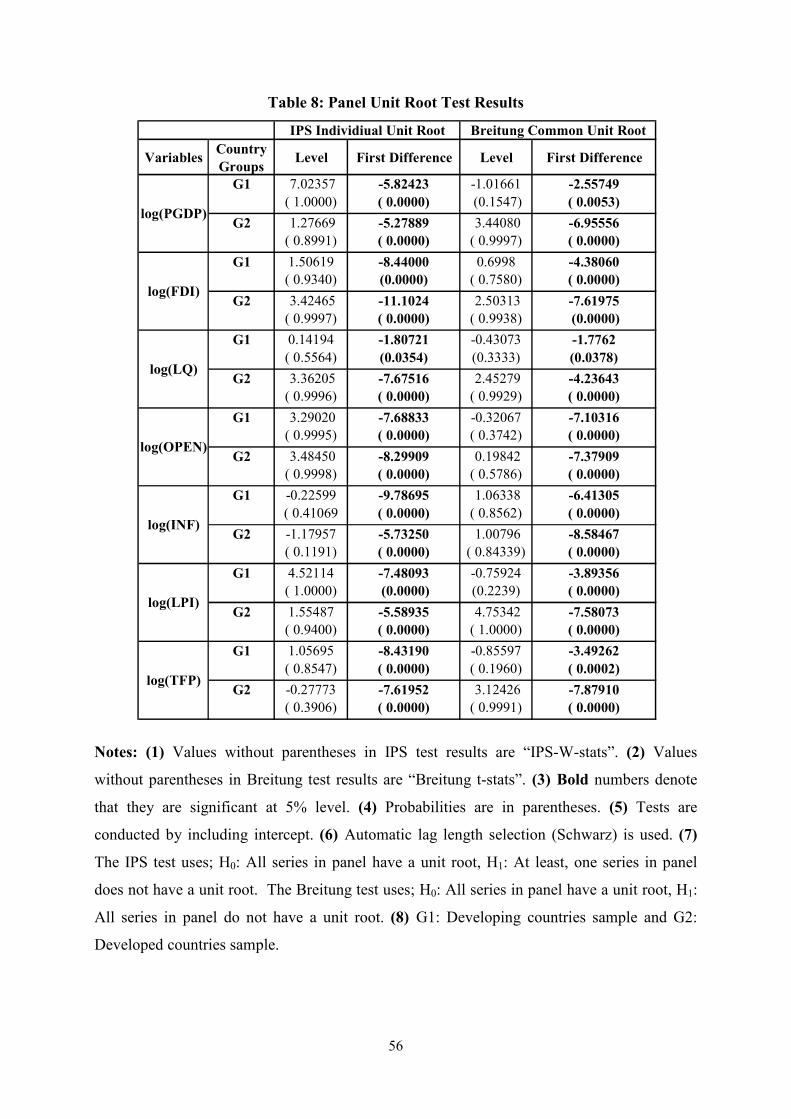
56

Table 8: Panel Unit Root Test Results

*otes: (1) Values without parentheses in IPS test results are “IPS-W-stats”. (2) Values

without parentheses in Breitung test results are “Breitung t-stats”. (3) Bold numbers denote

that they are significant at 5% level. (4) Probabilities are in parentheses. (5) Tests are

conducted by including intercept. (6) Automatic lag length selection (Schwarz) is used. (7)

The IPS test uses; H0: All series in panel have a unit root, H1: At least, one series in panel

does not have a unit root. The Breitung test uses; H0: All series in panel have a unit root, H1:

All series in panel do not have a unit root. (8) G1: Developing countries sample and G2:

Developed countries sample.

VariablesCountry

GroupsLevel First Difference Level First Difference

G1 7.02357( 1.0000)

-5.82423

( 0.0000)

-1.01661 (0.1547)

-2.55749

( 0.0053)

G2 1.27669( 0.8991)

-5.27889

( 0.0000)

3.44080( 0.9997)

-6.95556

( 0.0000)

G1 1.50619( 0.9340)

-8.44000

(0.0000)

0.6998( 0.7580)

-4.38060

( 0.0000)

G2 3.42465( 0.9997)

-11.1024

( 0.0000)

2.50313( 0.9938)

-7.61975

(0.0000)

G1 0.14194( 0.5564)

-1.80721

(0.0354)

-0.43073(0.3333)

-1.7762

(0.0378)

G2 3.36205( 0.9996)

-7.67516

( 0.0000)

2.45279( 0.9929)

-4.23643

( 0.0000)

G1 3.29020( 0.9995)

-7.68833

( 0.0000)

-0.32067( 0.3742)

-7.10316

( 0.0000)

G2 3.48450( 0.9998)

-8.29909

( 0.0000)

0.19842( 0.5786)

-7.37909

( 0.0000)

G1 -0.22599( 0.41069

-9.78695

( 0.0000)

1.06338( 0.8562)

-6.41305

( 0.0000)

G2 -1.17957( 0.1191)

-5.73250

( 0.0000)

1.00796( 0.84339)

-8.58467

( 0.0000)

G1 4.52114( 1.0000)

-7.48093

(0.0000)

-0.75924(0.2239)

-3.89356

( 0.0000)

G2 1.55487( 0.9400)

-5.58935

( 0.0000)

4.75342( 1.0000)

-7.58073

( 0.0000)

G1 1.05695( 0.8547)

-8.43190

( 0.0000)

-0.85597( 0.1960)

-3.49262

( 0.0002)

G2 -0.27773( 0.3906)

-7.61952

( 0.0000)

3.12426( 0.9991)

-7.87910

( 0.0000)

log(TFP)

log(LQ)

log(I*F)

log(PGDP)

log(OPE*)

IPS Individiual Unit Root Breitung Common Unit Root

log(LPI)

log(FDI)

57

Table 9: The Johansen- Fisher Panel Cointegration Test Results: Fisher Statistic from

Trace Test

*otes: (1) Values without parentheses are Fisher statistics from trace test. (2) Bold numbers

denote that they are significant at 5% level. (3) Probabilities are in parentheses. (4) Rank

column denotes the rank of cointegration; lag column denotes the number of lags is used for

the test. (5) Specification numbers are as in E-views 7. Specification No 2: Intercept in level

data (no trend), no trend and intercept in VAR. Specification No 3: Linear trends in level data,

not in VAR. Specification No 4: Intercept and linear trends in level data and no trend in VAR.

(6) The following null hypotheses are tested in turn: H0: r = 0, H0: r ≤ 1, H0: r ≤ 2, H0: r ≤ 3,

H0: r ≤ 4. (7) G1: Developing countries sample and G2: Developed countries sample.

Rank Lag Specification

*o

Model *o

and Variables

Country

Groups

tr (r=0) tr (r ≤ 1) tr (r ≤ 2) tr (r ≤ 3) tr (r ≤ 4)

G1 38.00

(0.0089)

26.20(0.1592)

1 1 3

G2 40.86

(0.0039)

16.33(0.6959)

1 1 3

G1 93.92

(0.0000)

35.81

(0.0162)

17.03(0.6510)

2 1 3

G2 126.1

(0.0000)

50.27

(0.0002)

20.42(0.4318)

2 2 4

G1 169.7

(0.0000)

74.17

(0.0000)

40.83

( 0.0039)

19.39(0.4967)

3 1 3

G2 174.3

(0.0000)

85.81

(0.0000)

49.57

(0.0003)

23.25(0.2767)

3 1 2

G1 319.9

(0.0000)

155.6

(0.0000)

71.11

(0.0000)

39.90

(0.0051)

21.75(0.3543)

4 1 2

G2 212.1

(0.0000)

115.8

(0.0000)

67.97

(0.0000)

32.70

(0.0181)

25.13(0.1214)

4 1 2

G1 36.44

(0.0136)

20.75(0.4119)

1 1 3

G2 52.73

(0.0001)

26.49(0.1503)

1 1 3

G1 113.7

(0.0000)

57.42

(0.0000)

18.39(0.5617)

2 2 3

G2 110.1

(0.0000)

56.10

(0.0000)

30.20(0.0666)

2 1 2

G1 38.71

(0.0072)

14.08(0.8265)

1 1 4

G2 32.49

(0.0384)

22.55(0.3113)

1 1 3

G1 71.44

(0.0000)

37.57

(0.0100)

22.46(0.3159)

2 1 3

G2 101.9

(0.0000)

44.06

(0.0015)

25.66(0.1773)

2 1 2

Fisher Stat. From Trace Test

Model 1:

log(PGDP),

log(FDI)

Model 2:

log(PGDP),

log( FDI),

log(LQ)

Model 3:

log(PGDP),

log( FDI),

log(LQ),

log(OPE*)Model 4:

log(PGDP),

log( FDI),

log(LQ),

log(OPE*), Model 5:

log(LP),

log(FDI)

Model 6:

log(LP),

log(FDI),

log(LQ)

Model 7:

log(TFP),

log(FDI)

Model 8:

log(TFP),

log(FDI),

log(LQ)

58

Table 10: The Johansen- Fisher Panel Cointegration Test Results: Fisher Statistic from

Max-Eigen Test

*otes: (1) Values without parentheses are Fisher statistics from max-eigen test. (2) Bold

numbers denote that they are significant at 5% level. (3) Probabilities are in parentheses. (4)

Rank column denotes the rank of cointegration; lag column denotes the number of lags is

used for the test. (5) Specification numbers are as in E-views 7. Specification No 2: Intercept

in level data (no trend), no trend and intercept in VAR. Specification No 3: Linear trends in

level data, not in VAR. Specification No 4: Intercept and linear trends in level data and no

trend in VAR. (6) The following null hypotheses are tested in turn: H0: r = 0, H0: r ≤ 1, H0: r ≤

2, H0: r ≤ 3, H0: r ≤ 4. (7) G1: Developing countries sample and G2: Developed countries

sample.

Rank Lag Specification

*o

Model *o

and Variables

Country

Groups

λ (r=0) λ (r ≤ 1) λ (r ≤ 2) λ (r ≤ 3) λ (r ≤ 4)

G1 33.57

( 0.0292)

26.2(0.1592)

1 1 3

G2 43.19

(0.0019)

16.33(0.6959)

1 1 3

G1 79.17

(0.0000)

36.45

(0.0136)

17.03(0.6510)

2 1 3

G2 96.35

(96.35)

46.95

(0.0006)

20.42(0.4318)

2 2 4

G1 120.6

(0.0000)

50.85

(0.0002)

40.05

(0.0049)

19.39(0.4967)

3 1 3

G2 109.7

(0.0000)

54.08

(0.0001)

46.22

(0.0008)

23.25(0.2767)

3 1 2

G1 205.5

(0.0000)

104.8

(0.0000)

49.70

(0.0002)

39.72

(0.0054)

21.75(0.3543)

4 1 2

G2 126.6

(0.0000)

62.00

(0.0000)

52.97

(0.0000)

24.31(0.1453)

25.13 (0.1214)

3 1 2

G1 36.37

(0.0139)

20.75(0.4119)

1 1 3

G2 49.81

(0.0002)

26.49(0.1503)

1 1 3

G1 77.53

(0.0000)

60.03

(0.0000)

18.39(0.5617)

2 2 3

G2 73.31

(0.0000)

46.81

(0.0006)

30.20(0.0666)

2 1 2

G1 40.92

(0.0038)

14.08(0.8265)

1 1 4

G2 32.31

(0.0401)

22.55(0.3113)

1 1 3

G1 51.90

(0.0001)

36.45

(0.0136)

22.46(0.3159)

2 1 3

G2 79.50

(0.0000)

37.50

(0.0102)

25.66(0.1773)

2 1 2

Model 5:

log(LP),

log(FDI)

Model 6:

log(LP),

log(FDI),

log(LQ)

Model 7:

log(TFP),

log(FDI)

Model 8:

log(TFP),

log(FDI),

log(LQ)

Fisher Stat. From Max-Eigen Test

Model 1:

log(PGDP),

log(FDI)

Model 2:

log(PGDP),

log( FDI),

log(LQ)

Model 3:

log(PGDP),

log( FDI),

log(LQ),

log(OPE*)Model 4:

log(PGDP),

log( FDI),

log(LQ),

log(OPE*),

59

Figure 2: Openness and FDI Relation in Developing Countries

Given country heterogeneity within our developing countries sample, as can be seen from the

regression line, there is a significant positive relation between openness and FDI stock/GDP

ratio. (Number of observations (N*T): 10*25= 250).

Source: Author’s own calculation.

-2

-1

0

1

2

3

4

-2.4 -2.0 -1.6 -1.2 -0.8 -0.4 0.0 0.4

log (OPEN)

log (FDI)