DEPARTMENT OF ACTUARIAL STUDIES

RESEARCH PAPER SERIES

The multi-binomial model and applications

by

Tim Kyng

Research Paper No. 2005/03 Division of Economic and Financial StudiesJuly 2005 Macquarie University Sydney NSW 2109 Australia

The Macquarie University Actuarial Studies Research Papers are written by members or affiliates of the Department of Actuarial Studies, Macquarie University. Although unrefereed, the papers are under the review and supervision of an editorial board.

Editorial Board: Piet de Jong

Leonie Tickle Copies of the research papers are available from the World Wide Web at: http://www.actuary.mq.edu.au/research_papers/index.html Views expressed in this paper are those of the author(s) and not necessarily those of the Department of Actuarial Studies.

THE MULTI-BINOMIAL MODEL AND APPLICATIONS

By Timothy Kyng, M Stats, M Ec, FIAA Lecturer in Actuarial Studies, Macquarie University, Sydney This paper develops a method for the valuation of multivariate contingent claims and is an extension of the well known binomial option pricing model. I refer to it as the Multi-Binomial Model. Structure of the paper:

1) Introduction

2) The problem the method is designed to address

3) examples of real world financial problems / multivariate contingent claims

4) analytic solutions and numerical solutions: the 1 dimensional

case

5) the multi-binomial method for valuation of contingent claims

6) examples / numerical results

7) conclusions

3

1) Introduction • The method presented is a numerical algorithm for the valuation of

contingent claims involving multiple, correlated, normally distributed , or lognormally distributed, sources of risk.

• The method constructs a discrete approximation to a correlated

multidimensional geometric Brownian motion process as the driving process which generates the amounts paid under the contingent claim being valued. It is a multidimensional “tree” approach to the valuation of contingent claims.

• Many such contingent claims are intractable when it comes to deriving

or using an analytic approach. • The methodology developed here can be applied to a wide range of

option pricing and contingent claims valuation problems. In particular it is applicable to valuation of executive share option schemes and valuation of complex exotic derivatives involving more than one asset, such as executive share option schemes, “spread options” and “rainbow options”.

• This numerical method is easy to program and is efficient and practical,

at least for low dimensional problems (up to about 5 assets). When the number of assets involved gets too big, it is better to use Monte Carlo Simulation.

• Various examples are included to illustrate the method.

4

2) The problem We have some financial contract or instrument or cashflow with • a payoff / cashflow made at time T, and • the payoff ( ) ( )( 1 ,..., n )f f S T S T= depends on the values of n different

variables ( ) ( )( )1 ,..., nS T S T . • These variables could be the values of n different asset prices observed

at time T. • Assume these are either normally or lognormally distributed • What is the expected value of the payoff / cashflow? • What is the present value of this expectation? • can we express the pv or expected value as some function g of the

initial values ( ) (( 1 0 ,..., 0nS S )) and some other variable? • Is an analytic solution available? If so is it easy to numerically

compute it? • Numerical solutions (e.g. Monte Carlo Simulation)

5

3) Examples of real world financial problems include: a. exchange option (option to exchange one risky asset for another) –

option to exchange 1 oz of gold (G) for 100 oz of silver (S) . . ( )max ,0T TPayoff S G= −

b. spread option (option on the difference between the prices of 2 risky

assets) where K is some constant. Even

if both S and G are lognormal, then the difference will have some other distribution (not lognormal) so a BS type formula will not apply. Alternatively instead of being an option contract S might be the assets and G the liabilities of an insurance company, so the payoff is the extent to which the surplus exceeds the level K.

max ,0T T

difference

Payoff S G K⎛ ⎞⎜= − −⎜ ⎟⎝ ⎠

⎟

c. 3-asset rainbow option (option on a portfolio of 3 assets R, S & V)

. ( )max ,0T T TPayoff R S V K= + + − d. Option defined on asset S at 3 different times ( )1 2 3, ,T T T and with the

payoff made at time T and is ( )( )

1 1 2 1 3

1 2 1 3

if S >S and S >S0 if S S or S ST

SV

⎧= ⎨ ≤ ≤⎩

where value of S at time i iS T= e. A 4-instrument payoff (option on a portfolio of long and short

positions in 4 assets R, E, A &L or the difference between a portfolio of 2 assets and 2 liabilities and some constant K.

[ ]( )max ,0T T T TPayoff R E A L K= − + − − .

6

4) Analytic and Numerical Solutions: The univariate situation (n = 1) Analytic solutions: For some types of payoff, there is an analytic formula. • The payoff from a European call option contract over the stock S, with

exercise price X, paid at time T is ( )max( ,0)payoff S X S X += − = − • The payoff from a put option contract over the stock S, with exercise

price X, paid at time T is ( )max( ,0)payoff X S X S += − = − Standard call and put options over a single asset can be valued using the well known Black and Scholes formula. This analytic formula applies only to options with European style exercise rights (those that can be exercised only on the maturity date of the contract). This formula expresses the value of the option in terms of the cumulative density function of the standard normal distribution. Black Scholes Formulae for European Options

1 2( ) ( )yT rTc Se N d Xe N d− −⎡ ⎤ ⎡= × − ×⎣ ⎦ ⎣ ⎤⎦

2 1( ) ( )rT yTp Xe N d Se N d− −⎡ ⎤ ⎡= × − − × −⎣ ⎦ ⎣ ⎤⎦ where • S = "spot price" (i.e. the current price) of the stock • X = the exercise price of the option • r = the risk free interest rate per annum • y = dividend yield (dividend paid p.a. as a proportion of the stock price) • T = term to maturity of the option • σ = volatility of the stock • c = value of a European call option • p = value of a European put option

21

1 1log2e

Sd r y TXT

σσ

⎡ ⎤⎛ ⎞ ⎛ ⎞= + − +⎜ ⎟ ⎜ ⎟⎢ ⎥⎝ ⎠ ⎝ ⎠⎣ ⎦ and 2 1d d Tσ= −

( ) ( ){ }21

21 Pr | ~ 0,12

xz

N x e dz z x z Nπ

−

−∞

= = <∫

7

From a statistical point of view, 1. the payoff / cashflow from an option is a random variable, and 2. the value of the option is the expected value of that cashflow,

discounted to a present value. The payoff depends on the distribution of the underlying asset (a stock). Under the Black Scholes Model, the logarithm of the price relative has a normal distribution:

It is assumed that 0

log Te

SS

⎛ ⎞⎜⎝ ⎠

⎟ follows a Brownian Motion process with drift

and has a normal distribution with

1. 212

mean r Tσ⎛ ⎞= −⎜ ⎟⎝ ⎠

2. 2variance Tσ= × These parameters define the so called “risk neutral distribution” of the asset price at any time T. This distribution is the one that makes the expected return on the asset S equal to the risk free interest rate r. Limitations of the BS formula: • it is not applicable to options that have early exercise features (can be

exercised before the maturity date) such as American options and Bermudan options.

• it is not applicable to many of the “exotic” options (those that are

different from a standard call or put option).

8

The one dimensional binomial model: One way to overcome some of the limitations of the BS model is to use the binomial model instead. In particular it allows us to • value american options and • other options with more complex payoffs than the standard call and

put options, in the case where the payoff depends on only one asset. This is a discrete time, discrete state space approximation to the value of an option. There are several ways to implement it. The most common is called the “Cox Ross Rubinstein” (CRR) version. We look at this first. Another way to implement it is the “equal probability” version of the model. The inputs to the model are (S, X, r, y, σ, T, m) Model assumes that the asset price can change only at discrete points in time. We break up the time interval [ ]0,T into m equally spaced time intervals

of length 1Tm

∆ = ×T . Time goes in steps of length T∆ .

At each time step the asset price can either go up or it can go down. The proportionate increase or decrease is constant: Either or 1t tS u+ = × S S1t tS d+ = × The u and d factors are constant at each time step.

• ( )expu Tσ= ∆

• ( )expd Tσ= − ∆

• ( ) ( )ln lnu d σ= − = ∆T The probability of an up step is ( )( ) ( )exp .p r T d u d= ∆ − −

9

For a European call option: ( ){ } ( ).max ,0 e r T

TE S X −− ×

−

The value of the option is which is a discounted conditional expectation:

( ) ( ) ( )( ). .0

0

e max ,0 1m

m kr m T k m k k

idiscountpayofffactor

probability

mvalue S u d X p p

k−− ∆ −

=

⎡ ⎤⎢ ⎥⎛ ⎞

= − ×⎢ ⎥⎜ ⎟⎝ ⎠⎢ ⎥

⎢ ⎥⎣ ⎦

∑

• this formulation of the option price as a discounted expectation shows

that we can value other more complicated payoffs – just replace the payoff function shown here with some other payoff function

It can be shown that as the number of time steps m gets bigger, the value of a call option given by this formula converges to the black scholes value Looking at the model statistically: • the stock price at time T (= time step m) after j up jumps in price is

0j m j

TS S u d −= . This takes values in the set { }0 : 0,1,..,k m kS u d k m− = • there are ( ) different values in this set (11m m+ = + )1

)

• The probability distribution of the asset value at time step m is

( ) ( )(0Pr 1 m kk m k kmS S u d p p

k−− ⎛ ⎞

= = −⎜ ⎟⎝ ⎠

for 0,1,...,k m=

• The probability distribution of the log price relative is

( ) ( ) ( )( ) ( )( )0Pr ln ln .ln 1 m kk

T

mS S m d k u d p p

k−⎛ ⎞

= + = −⎜ ⎟⎝ ⎠

• ( ) ( )( )

( )0ln ln

lnTS S m d

ku d−

= has a binomial distribution. It represents the

number of “up jumps” out of m “time steps”. • The log of the price relative has a transformed binomial distribution, it

is “log binomial” instead of “log normal”. The transformation is an “affine transformation” (a linear transformation plus a constant)

10

MOMENT MATCHING • The crr version of the model fixes the up and down movements (u,d)

and computes the probability p from the u and d . Parameters u, d and p are chosen in such a way that the probability distribution of the price relative has the right moments. In particular, the expected return on the asset is the risk free rate and the standard deviation of the log of the return is the volatility of the asset. This is the “risk neutral distribution”

• In order for the expected return on the asset to be the risk free rate, the

rate of price growth must be equal to the difference between the risk free rate and the dividend yield on the asset. The total return is comprised of the dividend yield and the capital gain return.

• The equal probability version of the model fixes the probability p to be

0.50 and computes the factors u and d so as to achieve “moment matching” to produce the “risk neutral distribution” of the asset price.

In option pricing there are various analytic and numerical methods used. These numerical methods involve • computing the expected value of the payoff • under the so called risk neutral distribution and then • discounting this expectation at the risk free rate. This is true of the bs model, the binomial model and various monte carlo simulation methods for valuation of options.

11

5) The Multi-Binomial Method for valuing Exotic Options For some multi-asset multi period exotic options, it is possible to derive an analytic valuation formula, in a Black-Scholes framework. These often involve the cdf of the multivariate normal distribution instead of the univariate normal distribution. The k dimensional multivariate normal cdf is the function

( )( ) ( ){ }

1 1,2 1,

1 1

,..., ; ,...,

Pr ,..., | , , ~ 0,1

k k k k

k i j ij i

N a a

Z a Z b corr Z Z Z N

ρ ρ

ρ

−

= < < =

• It is often quite difficult to derive an analytic formula for such a multi

asset option. Sometimes it is not possible to find one. • Even if an analytic formula exists, it may not be particularly useful

because it requires numerical computation of the multivariate normal cumulative distribution function.

• There exists a good numerical approximation for the 2 dimensional

normal cdf (known as drezner’s approximation). • However for higher dimensions, there is no good numerical

approximation and in practice monte carlo simulation is used to evaluate it.

12

Examples: 1) For the exchange option, an analytic formula exists. It is called the

“margrabe formula” and is really the bs formula “in disguise”. This is

possible because the ratio T

T

SG

is lognormal if both the numerator and

denominator are.

2) For the spread option ( where K is some

constant. Even if both S and G are lognormal, then the difference will have some other distribution (not lognormal) so a BS type formula will not apply.

max ,0T T

difference

Payoff S G K⎛ ⎞⎜= − −⎜ ⎟⎝ ⎠

⎟

)

3) Options on portfolios such as 3-asset rainbow option with

and a 4-instrument payoff such as (max ,0T T TPayoff R S V K= + + −

[ ](max ,0T T T TPayoff R E A L K= − + − − ) . The sum or difference of lognormally distributed variables is not lognormal so a BS type formula won’t apply

4) Option defined on asset S at 3 different times ( )1 2 3, ,T T T and the payoff

is made at time T and is ( )( )

1 1 2 1

1 2 1 3

if S >S and S >S0 if S S or S ST

SV

⎧= ⎨ ≤ ≤⎩

3 where value of S at time i iS T=

This one has an analytic formula

( )1 2 12 2 1 3 1

3 1

, ,r T T T Tvalue Se N T T T TT T

µ µσ σ

− − ⎛ ⎞−= − − − −⎜ ⎟⎜ ⎟−⎝ ⎠

where ( ) ( ) ({ )}2 1 2 1 2, , Pr , | , , ~ 0,iN a b Z a Z b corr Z Z Z Nρ ρ= < < = 1 this involves the cdf of the 2 dimensional normal distribution

13

UTILITY OF MULTI -BINOMIAL MODEL It is these types of problems which the multi-binomial model can value numerically. It is an alternative to monte carlo simulation when the dimension of the problem (the number of assets) is low (say less than 6). For higher dimensional problems, monte carlo simulation is more efficient. This method is applicable to a wide range of option pricing and other financial problems, such as 1) Executive share option schemes with performance hurdles. These are options where the payoff depends on • the share price of the firm at the maturity date, and • the absolute performance (rate of return) of the firm up to some time or

set of times • the relative performance of the firm (relative to other stocks, or to some

stock market indexes) up to some time or set of times. • other hurdles 2) spread options, rainbow options 3) asset liability studies where each of the assets and each of the liabilities

are lognormally distributed 4) multi asset options with early exercise features (these are more difficult

to value using monte carlo simulation)

14

The main result: Assume that we have • n assets, value at time t given by the vector: ( ) ( ) ( )( )1 2, ,..., nS t S t S t

These are assumed to be lognormal. • vector of returns ( ) ( )( ) ( ) ( )( )( )1 1ln 0 ,..., ln 0n nS t S S t S • this returns vector follows a correlated n-dim Brownian motion with

drift ( )( ) ( ). . : 1,..i

i i ii

dS tdt dW t i n

S tµ σ= + = .,

• The mean vector of the returns is assumed to be

2 2 21 1 2 2

1 1 1, ,...,2 2 2n n a

r q r q r q T Tµ σ σ σ⎛ ⎞⎛ ⎞ ⎛ ⎞ ⎛ ⎞= − − − − − − =⎜ ⎟ ⎜ ⎟ ⎜ ⎟⎜ ⎟⎝ ⎠ ⎝ ⎠ ⎝ ⎠⎝ ⎠µ ×

• The covariance matrix of the returns is assumed to be

21 1 2 12 1 1

21 2 12 2 2 2

21 1 2 2

...

...... ... ... ...

...

n n

n na

n n n n n

T T

σ σ σ ρ σ σ ρσ σ ρ σ σ σ ρ

σ σ ρ σ σ ρ σ

⎛ ⎞⎜ ⎟⎜ ⎟Σ = = Σ ×⎜ ⎟⎜ ⎟⎝ ⎠

Let nY R∈ be a n-dimensional iid binomial random variable with parameters m and probability p = 0.5 so that • the components of the vector Y are iid iY ~ ( ,0.50)iY bin m

• mean vector ( )1

1 ...2 2

1

nY

m mE Y Rµ⎛ ⎞⎜ ⎟= = × = ∈⎜ ⎟⎜ ⎟⎝ ⎠

• n×n covariance matrix 4 n nY

mS I×

= ×

15

Then there exists a matrix ( )m

A and a vector ( )mb such that the vector

( ) ( ) ( )m mmX A Y b= + has

• dimension n • mean vector ( )

aE X Tµ= ×

• covariance matrix ( )covY

X T= ×Σ The matrix A and the vector b are :

( ) ( )2m

TAm

⎛ ⎞= ×⎜ ⎟

⎝ ⎠Σ

( ) 1mb Aµ= − × Where • ( )Σ is a square root of the matrix Σ , defined to be a matrix L such

that 'L L× = Σ . One type of square root is the cholesky square root. • (1 1,...,1= ) is a vector of 1’s It can be shown that ( )lim mm

X→∞

is multivariate normally distributed with the

above mean vector and covariance matrix. • The vector ( )mX is an approximation to the vector of log price relatives. • The vector ( ) ( )( ) ( ) ( )( )1exp exp ,...,expmm nW X X= = X is an

approximation to the vector of price relatives • The vector ( ) ( ) ( ) ( ) ( ) ( )( )1 10 exp ,..., 0 expm nS T S X S X= n is an

approximation to the vector of prices at time T. This is approximately lognormally distributed. We can write this more compactly as ( ) ( ) ( )0 .expS T S X=

Note that r is the risk free rate of interest and is the dividend yield on asset i.

iq

16

Algorithm for pricing European style option prices For the n-dimensional, m step binomial model, we assume that: • the parameters , , , ,

aar m T µ Σ are known

• the initial values ( ) ( ) ( )( )1 20 , 0 ,..., 0nS S S are known, • the payoff (P) we are valuing happens at time T and is some function

( ) ( ) (( 1 2, ,..., nP ))f S T S T S T= of the n asset values at time T

Compute (2a

TA cholm

= × Σ )

Compute 1a

b T Aµ= − × Expectation = 0 For ( )0 1 ni to m= + 1− Compute n dimensional vector y Compute x Ay b= + Compute ( )expw x= i.e. ( ) ( ) ( )1 1 2 2exp , exp ,..., expn nw x w x w= = = x Compute ( ) ( )( ) ( ) ( )( )1 1 1,..., 0 ,...,n nS T S T W S W S T= n Compute ( ) ( ) ( )( )1 2, ,..., nPayoff f S T S T S T=

Compute ( ) ( ){ }1 11

1Pr ... ... ...2

nm

n nn

mmY Y y y

yy⎛ ⎞⎛ ⎞ ⎛ ⎞= = × ×⎜ ⎟⎜ ⎟ ⎜ ⎟

⎝ ⎠⎝ ⎠ ⎝ ⎠

expectation = expectation + Payoff×probability Next i

( )price = expectation exp -rT× This algorithm gives the price of the contingent claim as a discounted expected cashflow.

17

The vector b for arbitrage freeness: The vector b defined above makes the distribution of x have the right mean vector and covariance matrix. However the expectation of the vector w (which represents the price relatives) will not be what it should be for “arbitrage freeness”. We require that ( ) ( )ir q T

iE w e −= so that the expected rate of return on asset i is the risk free rate.

Let je be the n dimensional vector defined by 1,0,ji ji

i je

i jδ

=⎧= = ⎨ ≠⎩

.

This vector has a 1 in position j, and 0 everywhere else. Define the vector s by '

js A e= . The i-th component of this vector is the ith component of row j of the matrix A.

the choice ( )1

e 1ln2

ijAn

j ji

b m r q T m=

⎡ ⎤⎛ ⎞+= − ∆ − ⎢ ⎥⎜ ⎟

⎢ ⎥⎝ ⎠⎣ ⎦∑ for the components of

the vector b guarantees that ( )( ) ( )ln jE W m r q Tj= − ∆ and hence that

( ) ( )jm r q TjE W e − ∆= for all j = 1…n

This variable jW is the price relative for the jth asset in our model. The numerical difference between the value of the vector b computed in this way and the value computed the other way is usually small and as m gets bigger the 2 converge.

18

Comments on the above result 1) This is a n-dimensional extension of the well known binomial option pricing method. It is an extension of the “equal probability” version of the binomial model, not of the Cox Ross Rubinstein version. The CRR version fixes the size of the up and down movements (u and d) and then solves for the probability p of an up step. This version of the model is more difficult to generalise to more than one dimension. It can be generalised to 2 dimensions but it is difficult to go beyond 2. The equal probability version of the model fixes the probability of an up step to be 0.50 and then solves for the up and down movements per time step. This is much easier to generalise to n dimensions. We “solve” for either the probabilities or the up and down movements by doing “moment matching”. 2) The above result applies to European type options (those only exercisable at maturity and where the payoff depends on asset prices observed at maturity). However it can be extended to apply to options with early exercise payoffs and options where the payoff at time T depends on prices observed at some earlier time. 3) The b vector in the main result does not guarantee that the distribution of asset prices is “arbitrage free” but it is approximately arbitrage free and the approximation improves as m increases. The other formula for b does guarantee the model will match the moments of the arbitrage free distribution. This is a slightly more complicated expression but the numerical values it produces are very close to the values given by the first b-vector formula. 4) This uses an “affine transformation” of the n dimensional binomial distribution to model the vector of log price relatives. This is similar to what we do in the 1-dimensional binomial model.

19

6) Numerical Results / Testing the model The algorithm was tested by applying it to various multi asset options where it is possible to perform a valuation analytically. 1) We shall price an “exchange option” to exchange 100 oz of silver in return for 1 oz of gold. The payoff at maturity is ( )max ,0T Tpayoff G S= − The valuation assumptions are: 5 year term m = 60 time steps risk free rate = 10% p.a. asset div yield volatility drift rate initial price1 gold 0% 20% 4.00% $ 380.00 2 silver 0% 20% 4.00% $ 400.00 correlations 100% 70% 70% 100%

Results: expected payoff $ 59.73 option value using binomial $ 44.25 option value using analytic formula $ 44.21 Ratio of analytic price to binomial price 0.9991 2) We shall price a spread option on the difference between the values of 100 oz of silver and 1 oz of gold, with an exercise price of K= 20. The payoff at maturity is ( )max ,0T Tpayoff G S K= − − . This can’t be valued analytically by the BS formula. The valuation assumptions are as above. Results: option value using binomial $ 38.11

20

3) we shall price an option with payoff

( ) ( )max 380,0 max 400,0T Tpayoff G S= − + − This payoff can be valued analytically as the sum of 2 standard call options. Using the same valuation assumptions as above, the results are: binomial option value $324.66analytic value $324.60

4) we shall price an option with payoff ( )max 780,0T Tpayoff G S= + −

This is a 2 asset rainbow option. We value it using the same valuation assumptions as above, except that we vary the correlation assumption. This payoff can’t be valued analytically by the bs formula. When the correlation is very high (99%) the 2 asset portfolio behaves like a single asset so the option value ($324.53) is close to that in ex 3. When we change the correlation to 0% the option value drops to $311.92. 5) we price a 3 asset option with payoff

( ) ( ) ( )0 0max 1 1 ,0 max 2 2 ,0 max 3 3 ,0T T Tpayoff S S S S S S= − + − + − 0 This payoff is the sum of the payoffs on 3 standard call options, where the exercise price is equal to the initial asset price (“at the money calls”). This can be valued analytically, so it allows us to check the accuracy of the binomial method. The valuation assumptions were r = 6%, T = 0.25, asset (i) div yld volatility correl matrix 5 0.04 0.2 100.0% 90.0% 60.0% 3 0.01 0.4 90.0% 100.0% 80.0% 2 0.02 0.1 60.0% 80.0% 100.0% The analytic value is 0.5156. The binomial model value (using 30 time steps) is $0.5145. The ratio of these 2 values is 99.77%. If we change the payoff to the sum of 3 put option payoffs, then the analytic value is $0.4340 while the binomial value is 0.4328. The ratio is 99.73%

21

7) Concluding remarks: This paper has shown how to create a discrete approximation to the multivariate normal distribution and the multivariate lognormal distribution. This result is useful for option pricing applications and other financial applications involving correlated normal or lognormal variables. Because the number of calculations required is proportional to ( )1 nm + (where m = number of time steps and n = dimension), and this grows very quickly, the method is practical only for n up to about 4. It is an alternative to monte carlo simulation for low dimensional problems. The method covered here for option pricing can be extended to cover American style multi asset options and other options with early exercise features. The results shown also have applications to statistics and mathematics, as a way to numerically compute expected values of functions of a multivariate normal or multivariate lognormal random variable. In particular for n > 2, expectations and probabilities from these distributions have to be computed numerically anyway. This is an alternative way to do it. The results shown here also have academic applications, for generating discrete multivariate random variables with a specified mean vector and specified covariance matrix. This could be useful for creating examples for students to examine and work on. It has also shown how to compute expectations of functions of random variables with these distributions. Speed of computation is an issue with this method. However for many applications speed is not the only consideration. For an option dealer doing a deal on the phone, instant computation may be required but for many other situations it is not such a big issue.

22

Appendix 1: Detailed Numerical Example: The best way to understand the above result and algorithm is by working through a numerical example. We shall do a 4 step valuation of a 3 asset “rainbow option” with a term to maturity of 3 months. Assume we have an “at the money put option” over the value of a portfolio of 3 assets. The valuation details are:

T = 0.25, m = 4, 1 0.062516

Tm= = 0.25T

m=

r = 6% asset div

yield volatility drift

rate initial price

1 4% 20% 0.00% $5.002 1% 40% -3.00% $3.003 2% 10% 3.50% $2.00 $10.00

0.00000.03000.0350

aµ

+⎛ ⎞⎜ ⎟= −⎜ ⎟⎜ ⎟+⎝ ⎠

Correlation matrix 100% 90% 60% 90% 100% 80% 60% 80% 100%

Covariance matrix (annualised)

aΣ

0.040 0.072 0.012 0.072 0.160 0.032 0.012 0.032 0.010

Covariance matrix .

aTΣ = Σ

0.0100 0.0180 0.0030 0.0180 0.0400 0.0080 0.0030 0.0080 0.0025

23

Cholesky square root of annual cov matrix ( )achol Σ

0.200000 0.000000 0.0000000.360000 0.174356 0.0000000.060000 0.059648 0.053311 Computing the A matrix

(2a

TA cholm

= × Σ )

0.100000 0.000000 0.0000000.180000 0.087178 0.0000000.030000 0.029824 0.026656

Computing the b vector: We can compute the b vector so that the distribution of the vector X the vector of log price relatives, has the correct mean and covariance structure. This gives us

1a

b T Aµ= − × 0.0000 0.200000 0.000000 0.000000 10.0300 0.25 4 0.25 0.360000 0.174356 0.000000 10.0350 0.060000 0.059648 0.053311 1

b+⎛ ⎞ ⎛ ⎞⎜ ⎟ ⎜ ⎟= − × − × × ×⎜ ⎟ ⎜ ⎟⎜ ⎟ ⎜ ⎟+⎝ ⎠ ⎝ ⎠

⎛ ⎞⎜ ⎟⎜ ⎟⎜ ⎟⎝ ⎠

-0.200000-0.541856-0.164209

b⎛ ⎞⎜ ⎟= ⎜ ⎟⎜ ⎟⎝ ⎠

Alternatively we can compute the b the b vector so that the distribution of the vector X has the right covariance structure but the distribution of the vector (expW = )X has the correct mean vector (for the arbitrage free joint distribution of the n asset prices)

24

( )1

e 1ln2

isn

j ji

b m r q T m=

⎡ ⎤⎛ ⎞+= − ∆ − ⎢ ⎜ ⎟

⎝ ⎠⎣ ⎦∑ ⎥ where '

js A e=

For j = 1 we have ( )1 0 0je = and ( )' 0.1 0 0js A e= = and

( )

( ) ( )

1 11

e 1ln2

0.06 0.04 0.25 4 0.0512495+0+0 0.199998

isn

ib r q T m

=

⎡ ⎤⎛ ⎞+= − ∆ − × ⎢ ⎥⎜ ⎟

⎝ ⎠⎣ ⎦= − × − × = −

∑

For j = 2 we have ( )0 1 0je = and ( )' 0.18 0.087178 0js A e= = and

( )

( ) ( )

2 21

e 1ln2

0.06 0.01 0.25 4 0.094045+0.044539+0 -0.541833

isn

ib r q T m

=

⎡ ⎤⎛ ⎞+= − ∆ − × ⎢ ⎥⎜ ⎟

⎝ ⎠⎣ ⎦= − × − × =

∑

For j = 3 we have ( )0 0 1je = and

( )' 0.03 0.029824 0.026656js A e= = and

( )

( ) ( )

3 31

e 1ln2

0.06 0.02 0.25 4 0.015112+0.015023+0.013417 -0.164209

isn

ib r q T m

=

⎡ ⎤⎛ ⎞+= − ∆ − × ⎢ ⎥⎜ ⎟

⎝ ⎠⎣ ⎦= − × − × =

∑

Note that the numerical values in the b vector computed this way

0.199998-0.541833-0.164209

b−⎛ ⎞⎜ ⎟= ⎜ ⎟⎜ ⎟⎝ ⎠

are very close to the numerical values in the b vector computed in the other

way. -0.200000-0.541856-0.164209

b⎛ ⎞⎜ ⎟= ⎜ ⎟⎜ ⎟⎝ ⎠

Note also that the 3 s-vectors are the 3 rows of the matrix A

25

Sample Calculation at time step m=4 Consider time step m=4: the set of vectors / nodes at time step 4 is of size

( )3125 4 1= +• The 117th y vector is ( )1,3,4y = • The affine transformation x Ay b= + maps this vector to

( )-0.099998,-0.100299,0.061885x = • The exponentiation of x is ( )0.904839 0.904567 1.063841w = • The vector of asset prices at time step m=4 is thus

( )5 0.904839 3 0.904567 2 1.063841S = × × × • The value of the portfolio is

$9.3656 5 0.904839+3 0.904567+2 1.063841= × × ×• The put option payoff is ( ) max 10.0000-9.3656,0 0.6344=

• The probability of this payoff is 124 4 4 1 0.00390625

1 3 4 2⎛ ⎞ ⎛ ⎞ ⎛ ⎞⎛ ⎞= × × =⎜ ⎟⎜ ⎟ ⎜ ⎟ ⎜ ⎟

⎝ ⎠⎝ ⎠ ⎝ ⎠ ⎝ ⎠

The Option Price for a European Option The expected payoff at maturity (time step 4) is $0.4214. This is the sum of the products of payoff times probability across all 125 possible “nodes” in the “tree” at time step 4, i.e. the expectation at time step 0 of the payoff at time step 4. The value of the option using 4 time steps is $0.4151. This is the expected payoff at time step 4, discounted back to the valuation date (time step 0). If we increase the number of time steps to 20 the option price is $0.4139. If we increase the number of time steps to 30 the option price is $0.4134.

26

Appendix 2: Proofs It is well known that

1. ( ) ( ) ( ) ( )!~ , Pr 1! !

m yymY bin m p Y y p py m y

−⇒ = = −−

for 0,1,...,y m=

2. ( ) ( ) ( )e 1myt t

YM t E pe p⎡ ⎤= = + −⎣ ⎦ 3. if are iid then 1,..., nY Y ( ,bin m p)

( ) ( ) ( )1 11

!Pr ,..., 1! !

ii

nm yy

n ni i i

mY y Y y p py m y

−

=

⎛ ⎞= = = −⎜ ⎟

−⎝ ⎠∏

( ) ( ) ( )'

1 ,..., 11

,..., e 1i

n

n mtY tY Y n

i

M t t E pe p=

⎡ ⎤= = + −⎣ ⎦∏

( )( ) ( )( )1,..., 11

ln ,..., ln 1i

n

nt

Y Y ni

M t t m pe p=

⎡ ⎤∴ = +⎢ ⎥⎣ ⎦

∑ −

( )( )1,..., 11

1ln ,..., ln2

i

n

tn

Y Y ni

eM t t m=

⎡ ⎤⎛ ⎞+∴ = ⎢ ⎥⎜

⎝ ⎠⎣ ⎦∑ ⎟ when 0.5p =

4. Result from multivariate statistics (about moment generating functions and linear transformations): ( ) ( ) ( )' 'expx yx Ay b M t t b M A t= + ⇒ = 5 Define the vector je by ( ) 1,je i i j= = and ( ) 0,je i i j= ≠ . Then it

follows that ( ) ( ) ( ) ( )'expjx 'x j j y jE e M e e b M A e= = . We also have

'j je b b= and '

jA e = jth column of the transpose of A = jth row of A.

27

6. Let nY R∈ be a random variable with mean vector ( ) n

YE Y Rµ= ∈ and

n×n covariance matrix ( )covY

S Y= Let A be some constant n×n matrix and let nb R∈ be some constant vector Then the vector random variable X AY b= + has • dimension n • mean vector ( )E X A bµ= × +

• covariance matrix ( )cov T

YX A S A= × ×

7. Let S be a positive definite, symmetric n×n covariance matrix. Then

there exists a unique n×n lower triangular matrix L such that TL L S× = . Also the matrix L is invertible. This matrix L is known as the cholesky square root of the matrix ( )covS = Y

j>. Being lower triangular means that

so that the entries above the main diagonal are all zero. 0ijL for i= The notation ( )L chol S= means L is the cholesky square root of S Lemma

( ) ( )L chol S T L chol T S= ⇒ × = × for a constantT R∈

28

8. if are iid then we say that the vector 1,..., nY Y ( ,bin m p) ( )1,..., nY Y Y= has the binomial ( ), ,bin n m p distribution . The mean vector and

covariance matrix of this distribution are 12mµ = × and

4Y

m IΣ = ×

9. Affine Transformations and Moment Matching

Let Σ be a specified n×n positive definite symmetric covariance matrix Let nRµ∈ be some specified constant vector Let nY R∈ be a random variable with mean vector ( ) n

YE Y Rµ= ∈ and

n×n covariance matrix ( )covY

S Y= Then there exists a n×n matrix A and a vector nb R∈ Such that the affine transformation of the vector nY R∈ defined by X AY= + b has • dimension n • mean vector ( )E X µ= • covariance matrix ( )cov X = Σ The matrix A is defined by

( ) ( )1

1 2 1 2 YA L L where L chol and L chol S−= × = Σ = The vector b is defined by

Yb Aµ µ= −

29

10. Affine Transformation for equal probability binomial model Let nY R∈ be a n-dimensional binomial random variable with parameters m and equally likely probabilities so that

• mean vector ( )1

1 ...2 2

1

nY

m mE Y Rµ⎛ ⎞⎜ ⎟= = × = ∈⎜ ⎟⎜ ⎟⎝ ⎠

• n×n covariance matrix 4 n nY

mS I×

= ×

• the components of the vector Y are iid iY ~ ( ,0.50)iY bin m

• ( ) ( ){ }1 11

1Pr ... ... ...2

nm

n nn

mmY Y y y

yy⎛ ⎞⎛ ⎞ ⎛ ⎞= = × ×⎜ ⎟⎜ ⎟ ⎜ ⎟

⎝ ⎠⎝ ⎠ ⎝ ⎠

Then

( )2 2 n nY

mL chol S I×

= = ×

1

2

2n n

L Im

−

×= ×

( )1

1 2 1

2 2A L L L cholm m

−= = × = × Σ

( ) 1

1 1Y

b A m chol m Lµ µ µ µ= − = − × Σ × = − ×

The ith component of this vector is ( )11

,n

i ij

b m L iµ=

j⎡ ⎤

= − × ⎢ ⎥⎣ ⎦∑

30

Example: 2 dimensional case 2

1 12

1 2 2

2σ ρσ σρσ σ σ

⎛ ⎞Σ = ⎜ ⎟

⎝ ⎠ ( ) 1

1 22 2

0

1L chol

σ

ρσ σ ρ

⎛ ⎞= Σ = ⎜ ⎟⎜ ⎟−⎝ ⎠

11

1

2 21 2

1 0

11 1

Lσρ

σ ρ σ ρ

−

⎛ ⎞⎜ ⎟⎜ ⎟=⎜ ⎟−⎜ ⎟

− −⎝ ⎠

1 00 14

mS⎛ ⎞

= ⎜ ⎟⎝ ⎠

( )2

1 00 12

mL chol S⎛ ⎞

= = ⎜ ⎟⎝ ⎠

1

2

1 020 1

Lm

− ⎛ ⎞= ⎜ ⎟

⎝ ⎠

11

1 2 22 2

021

A L Lm

σ

ρσ σ ρ− ⎛ ⎞

= × = ⎜ ⎟⎜ ⎟−⎝ ⎠

1

2

µµ

µ⎛ ⎞

= ⎜⎝ ⎠

⎟ 112Y

mµ⎛ ⎞

= ⎜ ⎟⎝ ⎠

( )

112

2 2 2

112

2 2

0 12121

1

Y

mb Am

m

m

σµµ µ

µ ρσ σ ρ

σµµ σ ρ ρ

⎛ ⎞⎛ ⎞ ⎛ ⎞= − = − × × ×⎜ ⎟⎜ ⎟ ⎜ ⎟⎜ ⎟− ⎝ ⎠⎝ ⎠ ⎝ ⎠

⎛ ⎞⎛ ⎞ ⎜ ⎟= −⎜ ⎟ ⎜ ⎟+ −⎝ ⎠ ⎝ ⎠

( )1

12

22 1b m

σµσ ρ ρµ

⎛ ⎞⎛ ⎞ ⎜ ⎟= −⎜ ⎟ + −⎜ ⎟⎝ ⎠ ⎝ ⎠

31

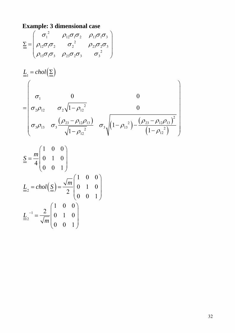
Example: 3 dimensional case 2

1 12 1 2 13 12

12 1 2 2 23 2 32

13 1 3 23 2 3 3

3σ ρ σ σ ρ σ σρ σ σ σ ρ σ σρ σ σ ρ σ σ σ

⎛ ⎞⎜ ⎟Σ = ⎜ ⎟⎜ ⎟⎝ ⎠

( )

( ) ( ) ( )( )

1

1

22 12 2 12

223 12 13 23 12 132

3 13 3 3 13 221212

0 0

1 0

111

L chol

σ

σ ρ σ ρ

ρ ρ ρ ρ ρ ρσ ρ σ σ ρ

ρρ

= Σ

⎛ ⎞⎜ ⎟⎜ ⎟⎜ ⎟

= −⎜ ⎟⎜ ⎟

− −⎜ ⎟− −⎜ ⎟⎜ ⎟−−⎝ ⎠

1 0 00 1 0

40 0 1

mS⎛ ⎞⎜ ⎟= ⎜ ⎟⎜ ⎟⎝ ⎠

( )2

1 0 00 1 0

20 0 1

mL chol S⎛ ⎞⎜ ⎟= = ⎜ ⎟⎜ ⎟⎝ ⎠

1

2

1 0 02 0 1 0

0 0 1L

m−

⎛ ⎞⎜ ⎟= ⎜ ⎟⎜ ⎟⎝ ⎠

32

( ) ( ) ( )( )

1

1 2

1

22 12 2 12

223 12 13 23 12 132

3 13 3 3 13 221212

0 02 1 0

111

A L L

m

σ

σ ρ σ ρ

ρ ρ ρ ρ ρ ρσ ρ σ σ ρ

ρρ

−= × =

⎛ ⎞⎜ ⎟⎜ ⎟⎜ ⎟

−⎜ ⎟⎜ ⎟

− −⎜ ⎟− −⎜ ⎟⎜ ⎟−−⎝ ⎠

1

2

3

µµ µ

µ

⎛ ⎞⎜ ⎟= ⎜ ⎟⎜ ⎟⎝ ⎠

11

21

Y

mµ⎛ ⎞⎜ ⎟= ⎜ ⎟⎜ ⎟⎝ ⎠

11

Yb A mµ µ µ= − = − L where 1 is vector of 1’s

The adjustment vector 11m L is subtracted from the vector

1

2

3

µµ µ

µ

⎛ ⎞⎜ ⎟= ⎜ ⎟⎜ ⎟⎝ ⎠

This adjustment is 1

21

3

1m Lσσ ασ β

⎛ ⎞⎜ ⎟= ⎜ ⎟⎜ ⎟⎝ ⎠

where 212 121α ρ ρ= + −

( )( ) ( ) ( )

( )2 2

23 12 13 23 12 13213 132 2

12 12

11 1

ρ ρ ρ ρ ρ ρβ ρ ρ

ρ ρ− −

= + + − −− −

Note that the sum of the squares of the components of &α β is 1.0

33

11. Algorithm for pricing European style option prices For the n-dimensional, m step binomial model, we assume that: • the parameters , , , ,

aar m T µ Σ are known

• the initial values ( ) ( ) ( )( )1 20 , 0 ,..., 0nS S S are known, • the payoff (P) we are valuing happens at time T and is some function

( ) ( ) (( 1 2, ,..., nP ))f S T S T S T= of the n asset values at time T

Compute (2a

TA cholm

= × Σ )

Compute 1a

b T Aµ= − × Expectation = 0 For ( )0 1 ni to m= + 1− Compute n dimensional vector y Compute x Ay b= + Compute ( )expw x= i.e. ( ) ( ) ( )1 1 2 2exp , exp ,..., expn nw x w x w= = = x Compute ( ) ( )( ) ( ) ( )( )1 1 1,..., 0 ,...,n nS T S T W S W S T= n Compute ( ) ( ) ( )( )1 2, ,..., nPayoff f S T S T S T=

Compute ( ) ( ){ }1 11

1Pr ... ... ...2

nm

n nn

mmY Y y y

yy⎛ ⎞⎛ ⎞ ⎛ ⎞= = × ×⎜ ⎟⎜ ⎟ ⎜ ⎟

⎝ ⎠⎝ ⎠ ⎝ ⎠

expectation = expectation + Payoff×probability Next i

( )price = expectation exp -rT× This algorithm gives the price of the contingent claim. The term “expectation” here is the risk neutral expected payoff

34

12. The vector random variable X AY b= + is a discrete model for the vector of logarithms of price relatives of the n assets. As the distribution of m →∞ X AY b= + converges to a multivariate normal distribution with mean vector

2 2 21 1 2 2

1 1 1, ,...,2 2 2n n a

r q r q r q T Tµ σ σ σ⎛ ⎞⎛ ⎞ ⎛ ⎞ ⎛ ⎞= − − − − − − =⎜ ⎟ ⎜ ⎟ ⎜ ⎟⎜ ⎟⎝ ⎠ ⎝ ⎠ ⎝ ⎠⎝ ⎠µ ×

covariance matrix

21 1 2 12 1 1

21 2 12 2 2 2

21 1 2 2

...

...... ... ... ...

...

n n

n na

n n n n n

T T

σ σ σ ρ σ σ ρσ σ ρ σ σ σ ρ

σ σ ρ σ σ ρ σ

⎛ ⎞⎜ ⎟⎜ ⎟Σ = =⎜ ⎟⎜ ⎟⎝ ⎠

Σ ×

This is true because of the central limit theorem. Each component of Y converges to a normal distribution, so Y converges to a multivariate normal. X being an affine transformation of Y also converges to a multivariate normal. It follows that asymptotically (m ), the vector →∞ ( )expw x= i.e.

( )exp , 1...i iw x i= = n converges to a multivariate lognormal distribution and that ( ) ( )( ) ( )( )exp expi i iE w E x r q T= = − This is the “arbitrage free joint distribution” of the n assets. However, being a discrete random variable, for m finite we have ( ) ( )( ) ( )(exp expi i )iE w E x r q T= ≈ − but the approximation improves in

accuracy as m gets bigger. We can use a different b vector here, which will guarantee that ( ) ( )( ) ( )(exp expi i )iE w E x r q T= = − for all values of m, so that the

model is “arbitrage free” for all values of m. The formula for the b vector is more complicated however.

35

The vector b for arbitrage freeness:

Let je be the n dimensional vector defined by 1,0,ji ji

i je

i jδ

=⎧= = ⎨ ≠⎩

Define the vector s by 'js A e=

By result 5 above we have ( ) ( )j jX byE e e M= s

by result 4 we have ( )( )1

1ln ln2

ij

SnX

ji

eE e b m=

⎡ ⎤⎛ ⎞+= + ⎢ ⎥⎜ ⎟

⎝ ⎠⎣ ⎦∑

It follows that the choice ( )1

e 1ln2

isn

j ji

b m r q T m=

⎡ ⎤⎛ ⎞+= − ∆ − ⎢ ⎥⎜

⎝ ⎠⎟

⎣ ⎦∑ for the

components of the vector b guarantees that ( )( ) ( )ln j jE W m r q= −

and hence that ( ) ( )jm r qjE W e −= for all j = 1…n

This variable jW is the price relative for the jth asset in our model.

Compute b from ( )1

e 1ln2

isn

j ji

b r q T m=

⎡ ⎤⎛ ⎞+= − − ⎢ ⎥⎜

⎝ ⎠⎟

⎣ ⎦∑ for all j = 1 … n

36