DELAMINATION ANALYSIS BY USING COHESIVE … delamination in laminated composites. In this study, ... Behavior used for cohesion analysis for quasi-brittle fracture

$Page 1: DELAMINATION ANALYSIS BY USING COHESIVE … delamination in laminated composites. In this study, ... Behavior used for cohesion analysis for quasi-brittle fracture$
DELAMINATION ANALYSIS BY USING COHESIVE INTERFACE ELEMENTS IN

LAMINATED COMPOSITES

A THESIS SUBMITTED TO

THE GRADUATE SCHOOL OF NATURAL AND APPLIED SCIENCES

OF

MIDDLE EAST TECHNICAL UNIVERSITY

BY

BURAK GÖZLÜKLÜ

IN PARTIAL FULFILLMENT OF THE REQUIREMENTS

FOR

THE DEGREE OF MASTER OF SCIENCE

IN

MECHANICAL ENGINEERING

AUGUST 2009

ii

Approval of the thesis:



submitted by BURAK GÖZLÜKLÜ in partial fulfillment of the requirements for the degree of

Master of Science in Mechanical Engineering Department, Middle East Technical University

by,

Prof. Dr. Canan Özgen _________________

Dean, Graduate School of Natural and Applied Sciences

Prof. Dr. Süha Oral _________________

Head of Department, Mechanical Engineering

Prof. Dr. K. Levend Parnas _________________

Supervisor, Mechanical Engineering Department, METU

Examining Committee Members:

Prof. Dr. Suat Kadıoğlu _________________

Mechanical Engineering Department, METU

Prof. Dr. K. Levend Parnas _________________


Assoc. Prof. Dr. Serkan Dağ _________________


Assoc. Prof. Dr. Altan Kayran _________________

Aerospace Engineering Department, METU

Dr. Demirkan Coker ________________

Aerospace Engineering Department, METU

Date: 27.08.2009

iii

I hereby declare that all information in this document has been obtained and presented in

accordance with academic rules and ethical conduct. I also declare that, as required by these

rules and conduct, I have fully cited and referenced all material and results that are not

original to this work.

Name, Last name: Burak Gözlüklü

Signature :

iv

ABSTRACT



Gözlüklü, Burak

M.Sc., Department of Mechanical Engineering

Supervisor: Prof. Dr. K. Levend Parnas

August 2009, 134 pages

Finite element analysis using Cohesive Zone Method (CZM) is a commonly used method to

investigate delamination in laminated composites. In this study, two plane strain, zero-thickness six-

node quadratic (6-NQ) and four-node linear (4-NL) interface elements are developed to implement

CZM. Two main approaches for CZM formulation are categorized as Unified Mode Approach

(UMA) and Separated Mode Approach (SMA), and implemented into 6-NQ interface elements to

model a double cantilever beam (DCB) test of a unidirectional laminated composite. The results of

the approaches are nearly identical. However, it is theoretically shown that SMA spawns non-

symmetric tangent stiffness matrices, which may lower convergence and/or overall performance, for

mixed-mode loading cases. Next, a UMA constitutive relationship is rederived. The artificial

modifications for improving convergence rates such as lowering penalty stiffness, weakening

interfacial strength and using 6-NQ instead of 4-NL interface elements are investigated by using the

derived UMA and the DCB test model. The modifications in interfacial strength and penalty

stiffness indicate that the convergence may be improved by lowering either parameter. However,

over-softening is found to occur if lowering is performed excessively. The morphological

differences between the meshes of the models using 6-NQ and 4-NL interface elements are shown.

As a consequence, it is highlighted that the impact to convergence performance and overall

performance might be in opposite. Additionally, benefits of selecting CZM over other methods are

discussed, in particular by theoretical comparisons with the popular Virtual Crack Closure

Technique. Finally, the numerical solution scheme and the Arc-Length Method are discussed.

Keywords: Delamination, Cohesive Zone Method, Finite Element Method, Double Cantilever Beam

Test, Arc-Length Method.

v

ÖZ

LAMINAT KOMPOZITLERDE YAPIŞKAN ARA ELEMAN KULLANILARAK

DELAMINASYON ANALIZI

Gözlüklü, Burak

Yüksek Lisans, Makina Mühendisliği Bölümü

Tez Yöneticisi: Prof. Dr. K. Levend Parnas

Ağustos 2009, 134 sayfa

Yapışkan Alan Metodu (YAM) kullanılarak gerçekleştirilen sonlu eleman analizi, laminat

kompozitlerdeki delaminasyonu incelemek için çok kullanılan bir metottur. Bu çalışmada, YAM’ nu

çalıştırmak için düzlem gerilim özellikli, sıfır yükseklikte altı-nodlu ikinci dereceli (6-Nİ) ve dört-

nodlu lineer (4-NL) iki arayüz elemanı geliştirilmiştir. YAM yaklaşımları Birleşik Mod Yaklaşımı

(BMY) ve Ayrık Mod Yaklaşımı (AMY) olarak sınıflandırılmış ve tekyönlü laminat kompozit yapılı

Çift Dirsekli Kiriş (ÇDK) testi modellemesinde kullanılmak üzere 6-Nİ arayüz elemanlarına

gömülmüştür. Yaklaşımlar için sonuçlar neredeyse aynıdır. Ancak, karışık-modlu yüklemelerde,

AMY asimetrik tanjant katılık matrislerinin oluştuğu teorik olarak gösterilmiştir ki bu da yakınsaklık

performansını ve/veya genel performansını karışık-modlu durumlarda düşürebilir. Takiben, BMY

yapısal denklemleri yeniden çıkarılmıştır. Ara-yüz dayanımının zayıflatılması, ceza sertlik

düzeyinin azaltılması ve 4-NL yerinde 6-Nİ ara-yüz elemanı kullanılması gibi yakınsaklık

performansını arttırıcı müdahaleler, çıkarılan BMY ve ÇDK testi modeli ile incelenmiştir. Ara-yüz

dayanımının zayıflatılması ve ceza sertlik düzeyinin azaltılması modifikasyonlarının etkileri

göstermiştir ki; herhangi birinin azaltılması durumunda yakınsaklık artabilmektedir. Ancak, fazlaca

azaltma durumda, aşırı-yumuşak sonuçlara ulaşılmıştır. 6-Nİ ve 4-NL arayüz elemanlarını kullanan

sonlu eleman modelleri arasındaki morfolojik farklılıklar gösterilmiştir. Bunun sonucunda,

yakınsaklık performansının ve genel performansın ters olarak etkilenebildiği ortaya konmuştur. Ek

olarak, YBM metodunun seçilmesindeki faydalar, diğer metotlar üzerinden, özelliklede iyi tanınan

Sanal Çatlak Kapama Tekniği ile teorik kıyaslama üzerinden tartışılmıştır. Son olarak, sayısal

çözümleme ve Eğri-Uzunluğu Metodu tartışılmıştır.

Anahtar Kelimeler: Delaminasyon, Yapışkan Bölge Metodu, Sonlu Eleman Metodu, Çift Dirsek

Kiriş Testi, Eğri-Uzunluğu Metodu.

vi

ACKNOWLEDGMENTS

The author wishes to express his deepest gratitude to his supervisor Prof. Dr. Levend Parnas for their

guidance, advice, criticism, encouragements and insight throughout the research.

The author would also like to thank Assoc. Prof. Dr. Gulio Alfano, from Brunel University, for his

suggestions and comments.

vii

TABLE OF CONTENTS

ABSTRACT ...................................................................................................................................iv

ÖZ ...................................................................................................................................................v

ACKNOWLEDGMENTS .............................................................................................................vi

TABLE OF CONTENTS ..............................................................................................................vii

LIST OF TABLES .........................................................................................................................xi

LIST OF FIGURES .......................................................................................................................xii

CHAPTER

1 INTRODUCTION ................................................................................................................ 1

1.1 Overview ........................................................................................................................ 1

1.2 Motivation ...................................................................................................................... 3

1.3 Objective ........................................................................................................................ 3

1.4 Content ........................................................................................................................... 4

2 REVIEW OF DELAMINATION PHENOMENON AND BACKGROUND ........................... 6

2.1 Cracks in Composites and Delamination.......................................................................... 6

2.2 Delamination Initiation Analysis ..................................................................................... 9

2.3 Delamination Propagation Analysis ............................................................................... 10

2.3.1 Cohesive Zone Method .......................................................................................... 11

2.3.1.1 A Brief History of CZM .................................................................................. 11

2.3.1.2 Studies Taken as Basis in the Study ................................................................. 12

2.3.1.3 Selected Studies about CZM ........................................................................... 13

2.3.1.4 Engineering Applications ................................................................................ 17

2.3.2 Fracture Mechanics Methods: Virtual Crack Closure Technique ............................. 19

2.3.2.1 VCCT vs. CZM .............................................................................................. 22

2.3.3 Other Delamination Analysis Methods ................................................................... 25

2.4 Failure Modes ............................................................................................................... 26

2.4.1 Mode I Fracture Mode ........................................................................................... 27

viii

2.4.2 Mode II Fracture Mode .......................................................................................... 33

2.4.3 Mode III Fracture Mode ......................................................................................... 34

2.4.4 Mixed-Mode Fracture ............................................................................................ 34

2.4.4.1 Initiation ......................................................................................................... 34

2.4.4.2 Propagation .................................................................................................... 35

3 COHESIVE ZONE METHOD DELAMINATION ANALYSIS ........................................... 40

3.1 Cohesive Zone Model ................................................................................................... 40

3.1.1 Definition of Cohesive Zone Length ....................................................................... 46

3.1.2 Griffith’s Theory in CZM ...................................................................................... 49

3.2 Mixed-Mode Cohesive Zone Model Derivation ............................................................. 51

3.2.1 CZM Constitutive Formulations for Mixed-Mode Failure ....................................... 54

3.2.1.1 Derivation of Tangent Stiffness Matrix............................................................ 58

4 CONVERGENCE ISSUE AND ARC-LENGTH METHOD ................................................. 63

4.1 Convergence Issue ........................................................................................................ 63

4.1.1 ―Trouble‖ in CZM and Literature Survey ............................................................... 63

4.1.2 Coping with Convergence Problem ........................................................................ 65

4.2 Arc-Length Method ...................................................................................................... 68

5 INTERFACE ELEMENT FORMULATION AND BENCHMARK TEST............................ 77

5.1 Finite Element Implementation ..................................................................................... 77

5.1.1 Shape Function Derivation for Quadratic Interface Element .................................... 78

5.1.2 Element Kinematics ............................................................................................... 80

5.1.3 Numerical Integration ............................................................................................ 85

5.2 Benchmark Test ............................................................................................................ 86

5.2.1 Finite Element Model of Double Cantilever Beam (DCB) Test ............................... 86

5.2.2 Finite Element Model ............................................................................................ 87

5.2.2.1 Model using 6-Node Quadratic Interface Elements .......................................... 88

5.2.2.2 Loading and Displacement Boundary Conditions ............................................ 91

5.2.2.3 Solution Procedure and Parameters ................................................................. 92

ix

5.2.2.4 Analytical Solution ......................................................................................... 93

5.3 Verification of Interface Element Implementation ......................................................... 94

6 RESULTS AND DISCUSSION ......................................................................................... 101

6.1 Comparative Analysis of Unified Mode Approach vs. Separated Mode Approach ........ 101

6.2 Investigation of Artificial Modifications for Improving Convergence ........................... 105

6.2.1 Comparative Analysis of Models Using 6-Node Quadratic and 4-Node Linear

Interface Elements ......................................................................................................... 105

6.2.2 Effects of Decreasing Interfacial Strength and Penalty Stiffness ............................ 107

6.3 Discussion on Convergence Performance .................................................................... 109

7 CONCLUSIONS ............................................................................................................... 112

8 FUTURE WORKS ........................................................................................................... 116

9 REFERENCES .................................................................................................................. 117

APPENDICES

A. Four Node Linear Interface Element Formulation and Model ............................... 126

B. Constitutive Relationship of Separated Mode Approach ....................................... 129

C. User Control in Arc-Length and Numerical Solution in MARC ............................ 132

CIRRICULUM VITAE ………………………………………………………………………...134

x

LIST OF TABLES

TABLES

Table 1: Different M values for plane stress approximation in literature [96] ............................. 47

Table 2: Material and interfacial properties of DCB test specimen in T300/977-2 [32] .............. 87

Table 3: Arc-Length solution parameters .................................................................................. 92

Table 4: Time and Increments to finish a job .......................................................................... 106

xi

LIST OF FIGURES

FIGURES

Figure 1: (a) Matrix cracks in different orientations (b) Micro crack movement in 0⁰ plies (c) H-

Splitting failure .......................................................................................................................... 7

Figure 2: Delamination inside a laminate .................................................................................... 8

Figure 3: Delamination initiation criteria .................................................................................... 9

Figure 4: (a) Dugdale/Barenblatt type cohesive zone stress-displacement profile (b) Typical

stress-displacement profile used for cohesion analysis for ductile fracture (c) Behavior used

for cohesion analysis for quasi-brittle fracture .......................................................................... 12

Figure 5: Mesh size and traction profile inside cohesive region ................................................. 14

Figure 6: Contact (upper) and friction (lower) features are highlighted by Yang and Cox .......... 15

Figure 7: SEM beam modeling with different discretizations. ................................................... 16

Figure 8: DCB test results obtained by using explicit FEA [98]................................................. 17

Figure 9: Crack closure method: step 1 — the crack is closed; step 2 — the crack is extended.

I — the intact area. .................................................................................................................. 20

Figure 10: Mesh sizes for the DCB model for (a) CZM (b) VCCT methods. ............................. 23

Figure 11: Initial delamination due to low velocity impact and predicted delamination propagation

used by CZM in a compressive loading .................................................................................... 24

Figure 12: Fringe plots with the damage parameter evolution ................................................... 25

Figure 13: Arbitrary crack propagation is allowed to move inside elements. .............................. 26

Figure 14: Uncoupled material and mesh feature resembling non-planar delamination

surfaces .................................................................................................................................. 26

Figure 15: Fracture modes ....................................................................................................... 27

Figure 16: Schematic illustration of DCB test. .......................................................................... 27

Figure 17: Fiber bridging during DCB test. .............................................................................. 28

Figure 18: R-curve effect on a DCB test of a (0º)24 CFRP laminate .......................................... 28

Figure 19: Strain energy release rate across width of DCB specimen at the crack front]. ............ 29

Figure 20: Evaluation of process zone at crack tip in a DCB test due to anticlastic effects. ........ 30

Figure 21: One of arms is treated as cantilever beam. ............................................................... 30

xii

Figure 22: Approximate analytical solution for DCB. ............................................................... 33

Figure 23: Mixed-Mode Bending (MMB) test .......................................................................... 35

Figure 24: DCB and ENF test correlation by superposition feature of MMB ............................. 36

Figure 25: Mixed-Mode and mode I, II failure criteria for an epoxy/graphite composite. ........... 37

Figure 26: Factor of η in Benzeggah and Kenane criterion, α for power law criterion and

corresponding fracture toughness values for various composites ............................................... 38

Figure 27: Various mode tests for AS4/PEEK carbon fiber unidirectional composite................. 39

Figure 28: (a) Bonding and de-bonding actions for the process zone (b) Top view of inner and

outer regions ............................................................................................................................ 40

Figure 29: (a) Dugdale model [36] in cohesive zone (b) Cohesive zone stress distribution by

Mi et al. [59]. ........................................................................................................................... 41

Figure 30: FE model and 3D interface elements in a DCB test specimen ................................... 42

Figure 31: Cohesive element relative displacement definition and separation of the surfaces. .... 42

Figure 32: Needleman's traction-displacement constitutive model, [66] (a) for Mode I and (b)

for Mode II (or Mode III). ........................................................................................................ 43

Figure 33: Various traction-displacement interface constitutive relations .................................. 44

Figure 34: Characteristics of constitutive relations (bilinear relationship). ................................. 44

Figure 35: Theoretical cohesive zone constitutive relationship with ―infinite‖ penalty stiffness. 46

Figure 36: Cohesive zone in the vicinity of crack and bi-linear constitutive relationship. (Not to

scale) ....................................................................................................................................... 47

Figure 37: Cohesive zone evolution as tip load increases for a DCB test model ......................... 49

Figure 38: Pure mode displacements in an interface element. .................................................... 51

Figure 39: Pure mode bilinear constitutive relationship. ............................................................ 52

Figure 40: Constitutive relationship for Mixed-Mode delamination........................................... 53

Figure 41: Constitutive relationship with unloading reveals irreversibility. ................................ 57

Figure 42: Constitutive relation minimum features. .................................................................. 61

Figure 43: (a) Snap Back (b) Snap Through (c) Brittle Collapse (d) Ductile Collapse cases ....... 64

Figure 44: Hybrid static/dynamic solution procedure on a snap-through region ......................... 65

Figure 45: (a) Mesh sensitivity load versus displacement results in application point for a finite

element model of DCB test using CZM [59] and 4x50 mesh size region (b) A close look for the

Snap-Back (S.B.) and Snap-Through (S.T.). ............................................................................. 66

xiii

Figure 46: Tip Load - Displacement curve for DCB test and interfacial strength effect [. ........... 67

Figure 47: Effect of penalty stiffness value K in a DCB test model with 2.5mm mesh size. ....... 67

Figure 48: (a) Newton-Raphson method iterates (b) Arc-Length method iterates ....................... 69

Figure 49: Principle of Arc-Length Method. ............................................................................. 71

Figure 50: Sign conventions for internal force and residual force and arc-length method

iterates. .................................................................................................................................... 72

Figure 51: Doubling back phenomenon and solution ................................................................ 74

Figure 52: Sharp-Snap Back with two possible roots ................................................................ 75

Figure 53: Crisfield’s spherical arc length method and Riks/Wempner’s linearized method ....... 76

Figure 54: 6-node quadratic interface element with nodes and integration points. ...................... 77

Figure 55: Grouping and node sets in 6-node quadratic interface element.................................. 79

Figure 56: Quadratic line element (The node sets on integration points is a rectangle with a

circle) ...................................................................................................................................... 79

Figure 57: Rotated interface element. ....................................................................................... 81

Figure 58: Possible misalignment angle configurations. ............................................................ 82

Figure 59: Nodal displacement vector in local coordinates. ....................................................... 83

Figure 60: DCB specimen dimensions. ..................................................................................... 86

Figure 61: Element 27, Plane Strain, 8-node Distorted Quadrilateral element. (―+‖:

Integration points, ―□‖: Nodes) ................................................................................................ 89

Figure 62: DCB model with zero thickness elements in model using 6-Node quadratic

interface elements. ................................................................................................................... 90

Figure 63: Loading and the displacement boundary conditions. ................................................ 91

Figure 64: Displacement vs. Increment input. ........................................................................... 91

Figure 65: Theoretical response ............................................................................................... 94

Figure 66: The model and the boundary conditions of standalone model for mode I test. ........... 95

Figure 67: Pure Mode check-run input and output. ................................................................... 96

Figure 68: The model and the boundary conditions of standalone model for mixed-mode test. .. 97

Figure 69: Mixed Mode (with β = 2.0) check run input and response ........................................ 98

Figure 70: Stress distribution in vicinity of crack tip. ................................................................ 99

xiv

Figure 71: Element Tangent Stiffness Matrix representation of UMA (for 6-node interface

elm.) ...................................................................................................................................... 102

Figure 72: Stiffness values in tangent stiffness matrix in UMA approach. (Openning

displacement is always kept as 0.0008 mm) ............................................................................ 103

Figure 73: Element Tangent Stiffness Matrix representation of SMA (for 6-node interface

elm.) ................................................................................................................................ 104

Figure 74: Absolute difference between a ―dotted‖ pink box and a ―clean‖ pink box for SMA. 104

Figure 75: Tip force versus displacement response of UMA and SMA. ................................... 105

Figure 76: Increment vs. required cycles for converganc of increment for element types ......... 106

Figure 77: Tip force vs Displacement response for 4 node linear and 6 node quadratic interface

elements ................................................................................................................................ 107

Figure 78: Tip Force - Displacement response of various interfacial strengths ......................... 108

Figure 79: Sensitivity results of penalty stiffness values.......................................................... 109

Figure 80: Cycle and Cutback segregation throughout the solution. ........................................ 110

Figure 81: 8-node element ―hatches‖ four 4-node elements with one additional node emerged

at the middle. ......................................................................................................................... 114

Figure 82: (a) 4-node linear plain strain interface element details (b) Node-set definitions ....... 126

Figure 83: Element 11, Arbitrary Quadrilateral Plane Strain Element (―+‖: Integration points,

―□‖: Nodes) ........................................................................................................................... 128

Figure 84: Compatibility of Mode I and Mode II .................................................................... 130

xv

1

CHAPTER 1

INTRODUCTION

1.1 Overview

Composite materials have gained popularity in high-performance products that need to be

lightweight, yet strong enough to withstand high loading conditions such as aerospace components,

boats, bicycle frames and racing car bodies. This is due to the fact that the technology combines

various materials with their unique characteristics so as to get a superior combination. However, the

complexity of the technology sometimes obstructs the understanding of failure modes and limits of

the structural parts. Unavoidably, the limits of the composite structures should be identified well in

order to use the technology efficiently and most importantly safely.

In the world of composites, Laminated Composites are the most widely used composites because of

the familiar manufacturing and performance characteristics. The main feature of laminated

composites is the stacking of laminas to ensure a global characteristic. Laminated composites are

customized for planar structures to attain high strength allowables. However, the resin rich layer

between the laminas has no reinforcement in through-the-thickness direction that sometimes yields

separation of the laminas, causing a crack called delamination crack or simply delamination.

Form of delamination damage is particularly insidious, since the delamination crack may propagate

undetected under the action of static or dynamic loads, leading to the ultimate failure of the

component in addition to inducing reductions in stiffness and compressive load-carrying capacity of

the laminate. Unlikely encountered in in-plane failures, the delamination would result in incapability

of the structure only in compressive strength. Therefore, it could not be revealed until a compressive

loading is applied at critical load or with special detection techniques. Consequently, the

delamination analysis literally attracts researchers in composite technology due to its insidious

characteristic.

Moreover, the delamination damage is frequently encountered in composite structures. A recent

survey on problems concerning composite parts of civil aircrafts shows that delamination, caused by

http://en.wikipedia.org/wiki/Aerospace

http://en.wikipedia.org/wiki/Bicycle

http://en.wikipedia.org/wiki/Racing_car

2

impact, presents 60% of all damage observed in composite structures [105]. In a 1991 IATA

(International Air Transport Association) survey, air carriers reported that about 40% of all damages

come from platform or ground handling and maintenance [105]. Hence, the ease of delamination

damage formation makes the phenomenon vital.

The delamination failure is predicted by using empirically determined design criteria – based on

maximum allowable stresses/strains– during layout and construction of components made of fiber

reinforced materials. For an optimal utilization, however, the potential offered by those materials as

well as for the determination of inspection intervals, it is also essential to predict propagation

delamination crack. In this study, the tool of Damage Mechanics is used for this purpose. This

methodology is unified with Fracture Mechanics that result in Cohesive Zone Method (CZM). In

this approach, the delamination surface is modeled between individual laminas by interface elements

of cohesive strengths which exhibit the approximate behavior of delamination cracks.

While the growth of delamination crack proceeds to the final, catastrophic failure, local changes in

material stiffness due to strain weakening and the formation of new free surfaces of subcritical

cracks are going to alter the load paths and result in load redistribution. The combined effects of the

damage processes generally lead to nonlinearity in macroscopic traction-displacement constitutive

relationships that are well defined by unique models called; Cohesive Zone Models. By embedding

these models, one may take the delamination into account by quasi-static finite element analysis. For

this purpose, MSC MARC 2005r3 [64] is used in the current study. Accordingly, appropriate

interface elements and formulations are developed. However, the numerical solution procedures are

the ones already included by MSC MARC.

The formulations of the cohesive interface elements comprise two main approaches encountered in

the literature. The first one is Seperated Mode Approach (SMA) considers mixed-mode delamination

phenomenon with individual pure modes as proposed by Mi et al. [59], Alfano and Crisfield [1]. The

next is the one considering the mixed-mode failure directly and actually, it is more widely used. It is

called Unified Mode Approach (UMA) used by Ortiz and Pandolfi [68], Allix and Corigliano [3] and

Camanho et al. [12]. These two concepts are theoretically compared in different mixed-mode ratios

in terms of convergence performance and accuracy for the analytical approximation. To do that, the

resulting tangent stiffness matrices formed by each approach are compared and contrasted.

In addition to the theoretical study, two finite interface elements are developed for numerical

implementation. The most widely used interface elements; six-node quadratic and four-node linear

elements, are both developed. In terms of accuracy and performance basis, two elements are

compared. The convergence improving methods which are decreasing penalty stiffness value and

3

weakening interface strength. The investigation performed in the above items is done by finite

element analysis of a unidirectional laminated composite Double Cantilever Beam (DCB) test.

1.2 Motivation

As mentioned in the introduction, delamination failure is a vital phenomenon that should be

investigated deeply. From initiation to propagation, CZM promises visualization, accuracy and

performance. In this sense, the capability of CZM makes it a senior candidate for the delamination

finite element analysis.

However, there are many interface element types, approaches, models and artificial modifications

that are all struggling to reach the most effective and accurate CZM interface element. On the other

hand, in industry, engineers, who would like to apply this method, cannot always know the best way

to use CZM. Therefore, a single CZM element, with both accurate and showing high performance in

convergence issue, should be reached. Therefore, the main motivation behind this study is to reach

most effective and accurate interface element addressing CZM.

1.3 Objective

The main objectives of this study are to develop and investigate CZM with interface finite elements

in laminated composites. For the achievement of the study, four-node linear and six-node quadratic

interface line elements with 2D plane stress assumption with zero-thickness capability are developed

and implanted into MSC MARC 2005r3.

Two different CZM formulation approaches are categorized and named as Separated Mode

Approach (SMA) and Unified Mode Approach (UMA). Both are theoretically compared in terms of

their resulting tangent stiffness matrices in various mixed-mode ratios. For the accuracy point of

view, both approaches are embedded into the developed six-node interface element and used in a

unidirectional DCB test finite element model. On the other hand, the characteristics of resulting

tangent stiffness matrices are investigated theoretically in order to point possible convergence

problems for other mixed-mode ratios, which is out-of-scope of the DCB test. From the results of the

theoretical and numerical comparison, one of the approaches is selected. The selected approach is re-

derived and implemented into both four-node and six-node interface elements in order to proceed to

further investigations. Both element types are applied into unidirectional DCB test model. The

results are compared in terms of accuracy and convergence performances of the elements. The

4

element showing higher performance is taken and the effects of interfacial strength and penalty

stiffness are investigated in order to find both accurate and high performance elements. Similarly,

the tests are performed in the same DCB model. Although the capabilities of the elements involve

mixed-mode loading, DCB test is selected in our study. The finite element analysis is performed in

Total Lagragian and the non-linear numerical solution technique is taken as the Spherical Arc-

Length method.

In addition to the above applications, the advantage of using Spherical Arc-Length Method is

discussed over Newton-Raphson method by stressing the importance of numerical solution scheme

of CZM applications. Also, the benefits of selecting CZM for delamination analysis are discussed

over other methods, especially by comparing with Virtual Crack Closure Technique (VCCT),

theoretically

1.4 Content

Chapter 2 is dedicated as the ―background‖ chapter of our study. This chapter investigates

methodologies for the analysis of delamination growth in terms of both types of approaches for other

procedures and CZM, respectively. In addition to the methodologies, contributing studies and

examples are stated and explained for the CZM. All these sections are constructed in a comparative

way among the methodologies and the example studies. However, the main emphasis is put on the

comparison of the well known Virtual Crack Closure Technique (VCCT) and the CZM. Secondly,

the delamination failure physics and the energy release rate in pure modes and mixed-mode are

discussed in this chapter. It also deals with the delamination phenomenon in a general point of view,

briefly. Yet, the main concern is the energy release rate in pure modes and mixed-modes.

Following the background chapter, Chapter 3 is devoted to the definitions and detailed discussion of

CZM. Explicitly, this is the main section in that the theory is discussed. Through a brief historical

background of CZM method, the theory and the physics behind the CZM is explained. Afterwards,

the formulations of UMA are derived once and in our way. In addition, the derivation of element

tangent stiffness matrix and internal force vector is presented. Regarding the method of UMA, the

approach of SMA is given in Appendix B.

The most challenging part of the CZM method is the non-linear solution scheme. In Chapter 4, this

problematic issue is tackled in a detailed manner. Besides, the method of arc-length is mainly

discussed and explained. The discussion is literally based on the comparison between the other

methods like well-known Newton-Raphson with the arc-length method. In addition to the analytical

5

point of view, since the arc-length method is selected as the nonlinear solver, thus, MSC MARC

2005r3’s capability of the arc-length method and the way user interfere with parameters are also

presented.

In Chapter 5, the element formulation of 6-node element with rotational capability is presented. The

numerical integration scheme is the key point in accordance with the internal force distribution and

tangent stiffness matrix. Therefore, the embedding section is discussed in detail. In addition, the

benchmark test of DCB, test finite element model and the boundary conditions are introduced.

In Chapter 6, the results of the benchmark test are investigated in the scope of the objectives of our

study. Finally, Chapter 7 is dedicated for the interpretation and Chapter 8 is for the further studies

planned.

6

CHAPTER 2

2 REVIEW OF DELAMINATION PHENOMENON AND BACKGROUND

In this section, the advantages and disadvantages of the CZM are presented by discussing over other

methods used in the literature for fracture mechanics simulations. In fact, this discussion puts the

CZM method inside the ―big picture‖ of the delamination simulation methods.

The delamination phenomenon is considered by categorizing the analysis types as delamination

initiation and delamination propagation. The initiation part is going to have brief discussion in the

way of presenting the methods that are proposed to be used. Since the propagation part is the main

concern in our study, this part would involve more detailed discussion. Particularly, the literature

survey for other methodologies is presented in this part.

In the explanation of the other methodologies, the main attention is given on the comparison with the

current method of CZM in a competitive way. Especially, Virtual Crack Closure Technique (VCCT)

is discussed and compared with CZM more elaborately since VCCT is the most popular method for

the delamination growth simulations. At the same time, VCCT is the typical application of Fracture

Mechanics (FM) based approaches [52]. Noting that FM methods are in competition with CZM,

hence, it would better to take them into account so as to criticize CZM method objectively.

One of the fundamental knowledge for our investigation is types of failure modes. Therefore, the

types of failure modes; mode I, mode II, mode III and mixed-mode phenomenon are explained,

especially, in the way of revealing their impacts to our study. Since the numerical simulation

performed is DCB test, analytical approximate solutions for mode I is given.

2.1 Cracks in Composites and Delamination

When a laminated composite panel is loaded, stresses are resolved excessively over inclusions or the

features like notches and holes. Unlikely observed in the isotropic crystalline materials, there are

various types of failures in composites. This is due to the heterogeneous structure of composites.

7

Therefore, it would be better to concentrate on typical cracks in composites and put the delamination

aside.

Recalling the structure of a laminated composite, the plane defined by a constituent lamina

corresponds to plane of laminate. Similarly, loads and stresses are ―in-plane‖ only if they are

applicable in that plane. For in-plane tension loading, there are various failure events possible to

occur. The first damage is generally the matrix failure, at the locations where a stress concentration

feature is located. One of those matrix failures could be matrix tensile cracking, especially in 90°

plies (in transverse loading direction). Another can be matrix shear cracking between fibers,

especially in off-axis 45° plies. In Figure 1a, one can distinguish 45° and 90° plies from the texture

and corresponding oriented cracks relating to the mentioned failures.

Figure 1: (a) Matrix cracks in different orientations (b) Micro crack movement in 0⁰ plies (c) H-

Splitting failure [105]

On the other hand for 0° plies, the matrix shear cracks may originate as microcracks, and run in

parallel between fiber pairs, in which they eventually become a splitting crack as shown in Figure

1b. Although these cracks are originated in the close vicinity of the stress concentrator features,

eventually they tend to move away from the stress concentrator edges, followed by running in the

direction of loadin. Consequently, H-type delamination is visible as illustrated in Figure 1c. Such

splitting cracks will be accompanied by delaminations between 0° plies and neighboring plies [105].

8

Hence, it can be noticed that even an in-plane crack may end up with a delamination. Unfortunately,

there are no such studies accompanying the possible interactions of different crack types.

For compressive loads, still the basic features of splitting and delamination crack development

process works, and still off-axis 45° plies are prone to have shear micro-cracking. Conversely,

tensile matrix cracking in 90° plies tends to be suppressed [105]. However, the failure is never

related to the fiber breakage in compressive loading. Instead of fiber failure, failure due to buckling,

either at the global or local level, generally happens [72].

The damage modes discussed so far are in-plane failure modes that stay inside the lamina or goes

through thickness of laminate. On the other hand, delamination failure corresponds to out-of-plane

failure which can be simply defined as ―debonding‖ of the constituent laminas resulting with

separation as shown in Figure 2.

Figure 2: Delamination inside a laminate

Although the resemblance of the delamination is a crack, delamination phenomenon is not treated as

easily as done for the in-plane cracks. For instance, the in-plane cracks are analyzed in terms of

stresses which can be found easily by Classical Laminated Plate Theory (CLPT). On the other hand,

the stresses are fully out-of-plane for the delamination cracks that would result in the surface

between laminas. Therefore, delamination analysis literally depends on so called interlaminar

stresses. Noting that, interface elements treat this phenomenon accurately as to be seen in the

following chapters dedicated for the finite element implementation.

From a different point of view, delamination cracks are more insidious than in-plane cracks. Such

behaviors make the delamination a dangerous phenomenon. The main reason for this conflict is

lacking of any reinforcement in through the thickness direction. As a result, delamination cracks are

9

easier to form. Also, the delamination does not influence the response if the loading is tension. This

characteristic makes the delamination insidious.

2.2 Delamination Initiation Analysis

Delamination initiation is generally analyzed by strength of material methods [95] which predicts

the onset of delamination by using interlaminar point-wise maximum stresses/strains [12]. One could

realize that the strength of material approach is a typical application that has been used so long for

in-plane failure modes, successfully. For out-of-plane crack, delamination, however, the approach

does not have such credibility because many experimental observations showed that using of a point-

wise stress/strain criterion is not sufficient [13].

Shear

Stress

Normal

StressσIc

σSc

Maximum Stress

Criterion

Quadratic

Interaction

Criterion

Camanho’s

Proposed

Criterion

σSc : Shear (Mode II&III) Allowable

σIc : Mode-I Allowable

Figure 3: Delamination initiation criteria

Generally, quadratic criterion [106] is most widely used in mixed-mode initiation problems as

shown in Figure 3. Besides, Camanho et al. [13,95] proposed a new criterion that seems more

delicate. This approach takes the total energy release rate, GT (GT = GI + GII + GIII) and the mixed-

mode effect into account in a different correlation. Noting that the quadratic criterion is the one used

in our study since it is most widely used and agreed method in literature. Particularly, this initiation

criterion is going to be discussed in detailed in the following sections.

Finally, an effective method has been developed as an amendment for the strength of material type

methods by introducing a versatile parameter, called characteristic length [105]. Unfortunately, this

10

approach cannot be efficiently used in engineering applications, because the characteristic length

parameter has not been proven to be a common material constant [105]. In other words, the length

scale is such an empirical parameter that it is supposed to be obtained by experiments with the same

stacking sequence.

2.3 Delamination Propagation Analysis

The other analysis type is delamination propagation which can be approached in two ways; the first

is based on the direct application of fracture mechanics, while the second formulates the problem

within the framework of damage mechanics. Although these two are the general approaches, there is

a relatively new method that can neither be classified in fracture mechanics nor in damage

mechanics types. This one is called Crack Tip Element (CTE) / non Singular Field (NSF) method

[25], basically based on the well known Classical Laminated Plate Theory (CLPT). Noticing that the

details for the damage mechanics method are not discussed in this section and the fracture mechanics

based methods will be discussed in detailed way under the umbrella of VCCT.

Delamination simulation procedures using FM, assume the existence of singular stress field around

delamination crack tip [12]. In FM methods, the propagation is to be expected when a function of the

energy release rates, GI, GII and GIII, along the delamination front locally exceeds a certain value,

[51,86,90] which is called fracture toughness, Gc. Actually, this value can be regarded as a property

of interface and depends on material and ply orientations of layers adjacent to the plane of

delamination [51].

The difference among FM methods generally depends on the way of performing calculation of strain

energy release rate [46,49,69,80,86]. For instance, VCCT calculates the energy release rate by using

Irwin’s crack closure integral [49], whereas, J-integral method [80], virtual crack extension [46], θ-

method [35] and stiffness derivative [69] use similar or modified procedures.

On the contrary, it is possible to directly calculate SIF (or stress field) by directly using Finite

Element Analysis (FEA) [90]. However, such direct FEM applications require specially designed

crack-tip elements, especially unavoidable for complicated geometries [90]. SIF-based methods

could be applied to predict the initiation of delaminations, and followed by any other method to

describe delamination growth as conducted in [51].

Recently, a third type of method other than FM or DM, Crack Tip Element (CTE) / non Singular

Field (NSF) type method has been developed by Davidson [25]. The method of CTE was developed

11

in order to deal with problems created by FM based methods. In the CTE/NFE method, the total

strain energy release rate is obtained from well-known Classical Laminated Plate Theory, directly.

The method is based on crack closure procedure that utilizes the near-tip plate theory in-plane forces

and moments along with stiffness matrices of the intact region and two cracked regions [25].

Therefore, CTE/NSF approach is based on the assumption that Classical Laminated Plate Theory

(CLPT) parameters completely characterize the near-tip loading and they are fully insensitive to the

details of the local damage. However, this methodology mainly depends on a parameter requiring

various tests that makes it hard to be applied in engineering applications easily. Even further,

CTE/NSF method is rather a new method and further analyses should be required.

2.3.1 Cohesive Zone Method

Although CZM is going to be discussed in the dedicated chapter elaborately, for the general view of

delamnination analysis, the studies in the field of CZM are given. Moreover, in this section, the

applications of Cohesive Zone Method (CZM) and distinguished studies are mainly discussed. Also,

the main objective is to show the ―big-picture‖ in that the cohesive zone modeling is more than

capable to be used in engineering applications.

2.3.1.1 A Brief History of CZM

There was no model defining the actual crack tip behavior before the end of 50s. Up to that date,

researchers had been using Linear Elastic Fracture Mechanics (LEFM) methods that assume an

abrupt transition from stress free crack surface to the bulk material. Later, Dugdale [36] remarked

thin plastic zone that is generated in front of the notch. Following Dugdale’s work, Barenblatt [15]

introduced cohesive forces on a molecular scale in the zone that Dugdale had pointed out in order to

solve the problem of equilibrium in elastic bodies with cracks in the way of the strength of the zone.

In 1976, Hillerborg et al. [48] proposed a model similar to the Barenblatt model; however, the

concept of tensile strength was introduced instead of molecular scale solution. Hillerborg’s model

allowed existing cracks to grow and, even more importantly, allowed the initiation of new cracks,

[48]. Actually, Hillerborg named the model as fictious crack model which interestingly recalls the

analogy of today’s interface element method. Actually, this was the stage, cohesive zone method was

assumed to be born.

12

(a) (b) (c)

Figure 4: (a) Dugdale/Barenblatt type cohesive zone stress-displacement profile [59] (b) Typical

stress-displacement profile used for cohesion analysis for ductile fracture [29] (c) Behavior used for

cohesion analysis for quasi-brittle fracture [29]

The concept of CZM has been used by Needleman [66] to simulate fast crack growth in brittle

solids. Needleman considered that cohesive zone models are particularly attractive when interfacial

strengths are relatively weak compared with the adjoining material, as is the case in composite

laminates. Unfortunately, the cohesive zone method has been used for the delamination of composite

materials after mid 90’s. Yet, the application based on the interface element formulation in finite

element analysis is more recent.

2.3.1.2 Studies Taken as Basis in the Study

The studies taken as basis should possess robust formulations. Fulfilling that requirement, the

following studies are the main ones that are taken as the main basis in our study.

One of the methods used in our study is proposed by Mi et al. [59] who performed CZM for the

analysis of delamination in fiber composites. Mi et al. proposed the well known method for the

mixed mode delamination in the scope of damage mechanics and indirectly using fracture mechanics

in which the damage is defined as an irreversible time parameter which was maintained during the

solution. The study is applied in the Double Cantilever Beam (DCB) test, the overlap specimen and

Mixed Mode Bending (MMB) test by using finite element model for the capability and the reliability

of the method. Consequently, the mixed mode interaction is analyzed. Typically, they compared the

results with the analytical ones and the results showed quite good results. In addition, Mi et al.

initiated discussions on the mesh size effect and the convergence related issues. Paralleling, they

suggested and used the most effective non-linear solution method that is modified cylindrical arc-

length method [19].

In the highlight of the study of Mi et al. [59], Alfano and Crisfield [1] have revisited CZM in a quite

extensive manner. They have revisited the previous work of Mi et al. to make it more robust,

13

especially in the tangent stiffness matrix derivation from the constitutive relation. The constitutive

relation is analytically related to all of the stages of the damage from initiation to the full separation.

Even, the formulation became capable for both loading and reloading in any phase of the damage.

Actually, the point they all consider the constitutive relationship is in pure mode displacements and

critical energy release rate. Hence, our study refers their work as Separated Mode Approach (SMA).

On the other part, Camanho et al. [13] used CZM in terms of total displacement which works as a

damage parameter at once. In addition to the former method, Camanho and Dávila [12] proposed a

CZM model that uses Benzeggagh-Kenane (BK) type mixed-mode delamination growth criterion.

Actually, as a contrast to SMA, Camanho et al. consider the formulation in terms of mixed-mode

displacements and critical energy release rates, our study refers their approach as Unified Mode

Approach (UMA). Also, it should be noted that there are many other authors [4,66,68] who have

been already using this approach.

2.3.1.3 Selected Studies about CZM

Besides the studies taken as basis for our study, there are numerous works for enhancing and

contributing to CZM. Moreover, it can be realized that the majority of the following studies are to

enhance the convergence rates since perhaps this is a vital problem for CZM.

Following the studies [59] and [1], Alfano et al. [72] has augmented co-rotational formulation into

the CZM method for the cases where there are large displacements and large rotations as seen in

highly nonlinear cases like buckling. In fact, the formulation of CZM is based on the small strain

approach. However, the delamination is a failure that generally there would be large displacements

during the simulation that would yield considerable element coordinate rotations during numerical

iterations. Consequently, the resulting element stiffness matrix would involve initial stress stiffness

matrix in which the variation of transformation matrix cannot be neglected. Actually, the tangent

stiffness matrix defined here is referred as consistent tangent stiffness matrix. To do that, they place

a local coordinate frame on the interface element nodes in such a way that as the element rotates with

the element, the coordinate frame rotates. As a result, Alfano et al. [72] has implemented the co-

rotational formulation and applied it successfully in the buckling simulations. Our study does not use

the co-rotational formulation since higher order terms can be neglected for the delamination growth

in a simple DCB test.

Qui et al. [15] embedded the study of Mi et al. [59] to analyze the convergence effects by artificially

varying the critical displacements instead. In fact, their study focuses on the application, detailed in

14

FE codes like finite element implementation and resulting influence to convergence. Therefore, this

study has great contribution for our study as far as the implementation to FEA code is concerned.

One of the novel contributions interpreting the popular convergence issue is perhaps the study of

Turon et al. [96]. According to their findings, the convergence problem mainly depends on the mesh

density in the cohesive zone region as going to be examined in the following chapters. However,

there is no accurate suggestion or requirement about the magnitude of the mesh density. Hence, they

proposed an accurate mesh density related to the dimensions of cohesive zone. Their suggestion is

illustrated in Figure 5 where it can be realized that the traction profile cannot be ―reached‖ unless

there is more than two elements. In addition to mesh density, one of the critical parameters affecting

the numerical solution scheme is the penalty stiffness, which was also examined.

Figure 5: Mesh size and traction profile inside cohesive region [96].

In terms of the convergence issue, Harper and Hallet [43] analyzed the mesh size and the cumulative

effect of interfacial strength. Their unique remark is about the interfacial strength that can be

decreased artificially in the favor of convergence performance. However, as a limitation to that

―trick‖, Harper and Hallet [43] showed that there is literally a limit for the amount of decrease in the

interfacial strength. They showed that excessively low interfacial strengths would affect the global

response that even result over-softening of the structure. Therefore, they highlighted that the

lowering of interfacial strength should be carefully done. Moreover in their study, for the first time,

the length of the numerical cohesive zone was investigated in detail and compared to analytical

solutions across a range of material and geometric parameters. As a result, a clear distinction was

drawn between the physical and analytical cohesive zone lengths, and that is resulting from a

numerical representation using interface elements.

15

The numerical solution scheme directly affects the convergence rates since the softening behavior of

CZM method would yield sharp-snap backs. A quite extensive discussion about non linear solution

procedures are considered by Alfano and Crisfield [2]. The key approach is enhancing the arc-length

method, which is achieved by localized control. In addition to the locally controlled arc length

method, advanced applications of line search methods are proposed. Single Line Search Method and

Double Line Search Method are also considered.

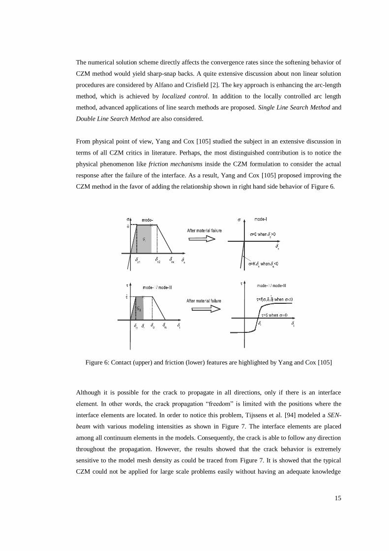
From physical point of view, Yang and Cox [105] studied the subject in an extensive discussion in

terms of all CZM critics in literature. Perhaps, the most distinguished contribution is to notice the

physical phenomenon like friction mechanisms inside the CZM formulation to consider the actual

response after the failure of the interface. As a result, Yang and Cox [105] proposed improving the

CZM method in the favor of adding the relationship shown in right hand side behavior of Figure 6.

Figure 6: Contact (upper) and friction (lower) features are highlighted by Yang and Cox [105]

Although it is possible for the crack to propagate in all directions, only if there is an interface

element. In other words, the crack propagation ―freedom‖ is limited with the positions where the

interface elements are located. In order to notice this problem, Tijssens et al. [94] modeled a SEN-

beam with various modeling intensities as shown in Figure 7. The interface elements are placed

among all continuum elements in the models. Consequently, the crack is able to follow any direction

throughout the propagation. However, the results showed that the crack behavior is extremely

sensitive to the model mesh density as could be traced from Figure 7. It is showed that the typical

CZM could not be applied for large scale problems easily without having an adequate knowledge

16

about the possible crack propagation directions. Therefore, this study is very important because of

remarking a lacking that might be come on the surface in three dimensional crack propagation

analyses.

Figure 7: SEM beam modeling with different discretizations [94].

Another major aspect of the methodology is perhaps the implementation process inside finite

element codes. Although our study and most of the studies so far are performed via implicit finite

element solvers, there are also numerous applications that use explicit solvers [71,98]. In fact, the

implementation into explicit FE packages has various advantages over the implicit ones. Actually,

one major advantage is the convergence rate in which the numerical integrations would take place

referring to time. However, there are two problems for embedding in explicit solvers [71,98]. The

first one is the oscillations around the equilibrium curve as seen from Figure 8. The second problem

actually arises due to the great convergence feature itself in that uses very small time steps that make

sometimes hard to analyze an engineering problem. Although such problems occur, explicit

applications are widely used, successfully.

17

Figure 8: DCB test results obtained by using explicit FEA [98].

Moreover, the interface elements could be modeled as springs as done by Wisnom and Chang [77]

for analyzing notched cross ply 0/90 laminates. They modeled splitting cracks and associated

delaminations by using plane stress elements in FEM formulations to represent plies and nonlinear

spring elements to represent crack wake processes. The spring elements were assigned a simple

constitutive law, consisting of an initial linear rising part, a constant regime, and an abrupt loss of

traction at a critical shear displacement. Yet, since out-of-plane stresses were not considered, the

spring elements were consistently restricted to imposing shear tractions to oppose sliding crack

displacements. Thus mode II and III crack displacements were possible, but not mode I. Similar to

the spring modeling of interface [77], the interface elements could be modeled as rods that were

suggested by Shahwan and Waas [89]. They proposed an interface model that could be used for

compressive loading without characterizing the problem whether it is a buckling, post-buckling or

static, conservatively. Moreover, the study was specialized for non self similar crack growth.

However, the most distinguishing feature of the study is that the interface elements only require the

mechanical properties (stiffness, thickness, etc.) of the laminate. They are adequate to totally

characterize cohesive processes without resorting to any external criteria such as those from fracture

mechanics concepts.

2.3.1.4 Engineering Applications

Today, nearly all well known commercial finite element packages have the cohesive element

capability with appropriate 2D and 3D elements. Therefore, either pioneering applications or novel

applications are going to be mentioned in this section.

18

Firstly, De Moura et al. [31] conducted the CZM method inside a low impact damage test resulting

in delamination. They used 3D interfacial element with a rectangular specimen where the

delamination is a ―pea-nut‖ type at the corner of the specimen. Indeed, this study [31] is based on

revealing the residual strength after the impact. Their main contribution is being the first study that

CZM method has been embedded in an engineering application where the delamination growth is

not a self similar one. In addition to this study, Aoki et al. [6] have also studied damage

accumulation mechanism in cross-ply Composite Fiber Reinforced Fiber (CFRP) laminates by the

low velocity impact.

As being one of the pioneering applications, Chen et al. [14,16] applied cohesive method in a

repaired sandwich and stiffened panel which are all modeled and analyzed by using CZM interface

elements. They showed that the methodology is capable to work well in actual engineering

problems. The results showed that widely used bilinear constitutive relationship agrees quite well

with test results. In addition, they noticed the effects of fracture toughness and interfacial strength

effect to the global response just like done for the basic tests like DCB and MMB. Similarly, T.-S

Han et al. [42] investigated feasibility of applying the cohesive crack propagation model as a method

to simulate delamination propagation between a facesheet and a core in a honeycomb panel.

Instead of 3D brick interface elements, Davila et al. [27] suggested to use interface shell elements,

modeled at the neutral planes of the plies, in 3D analysis. The shell cohesive elements have the same

topology as three-dimensional elements, thus; they can be generated using any finite element pre-

processor while zero-thickness cohesive elements for three dimensional elements cannot be

generated with most pre-processors. In addition, the shell element modeling decreases the processing

time of the finite element solver. The proposed model is applied to composite lugs and successful

results are obtained.

In addition to the static loading, there are many applications of CZM modeling for fatigue crack

growth in composite materials [11,83]. For instance, Robinson et al. [83] defines damage parameter

– cycle relation that is mimicking well known Paris-Erdogan type crack equation. Since the damage

is correlated with the cycles, it could be possible for the delamination to grow in the same manner as

in isotropic materials.

There are various applications where different kinds of materials are analyzed as to be used in

different engineering fields. For instance, Xu and Needleman [103], de Borst [37] and Elicses et al.

[28] studied the fracture in concrete materials and macromolecular based polymer materials by using

CZM method. Furthermore, Wei and Hutchinson [99], Thouless and Yang [104] applied the method

for adhesively bonded joints. In addition, for bi-material interfaces Needleman [65] and Tvergaard

19

and Hutchinson, [97] applied the CZM successively and for the dynamic fracture of homogeneous

materials, Needleman [66] studied the issue.

2.3.2 Fracture Mechanics Methods: Virtual Crack Closure Technique

Perhaps the most widely and successfully used technique for the delamination propagation is the

Virtual Crack Closure Technique (VCCT) [52]. Also, since VCCT can be thought as

―representative‖ of FM type methods, in order to compare damage mechanics method with fracture

mechanics type methods, it would be convenient to discuss VCCT in more detailed manner. Noting

that, the formulations given here is for the sake of showing the simplicity of the method. Moreover,

after discussing VCCT, VCCT and CZM methods will be compared more objectively.

As an application of FM, Rybicki and Kanninen [86] have developed VCCT in which the procedure

is mainly based on the calculation of the strain energy release rates at the crack tip [56]. VCCT is

based on the same assumption of Irwin’s crack closure integral [49], in which the energy released in

the process of crack expansion is equal to work required to close the crack to its original state as the

crack extends by a small amount [67]. Actually, the direct application of the Irwin’s crack closure

integral is generally referred as crack closure method [55].

The method has the assumption of non-altering state of the crack tip [86]. In words, the crack should

grow in a self-similar manner when the crack extends from a+Δa to a+2Δa [55]. Therefore, the crack

front is not allowed to be changed during the propagation. Under the scope of this requirement, the

energy release rates can be computed from the nodal forces and displacements obtained from finite

element model [13]. From Figure 9, the virtual work done by the force can be written as [52];

)(2

1luE δδF

(1)

20

Figure 9: Crack closure method: step 1 — the crack is closed; step 2 — the crack is extended. I — the intact area.

For the energy release rate, the previous equation becomes, [52];

1

2

EG

A A

u lδ -δ

F

(2)

where ΔG is the total energy release rate, ΔA is the crack surface created and F is the force to close

the crack, δu is the displacement for the upper node and δl is the displacement for the lower node.

Therefore, just by comparing the energy release rate with the critical value, the crack would

propagate accordingly.

The self-similar crack growth requirement spawns complicated remeshing algorithms in order to

keep the mesh in the crack tip to be able to move in the available directions [24,64]. Moreover, the

mesh in the VCCT region should be very refined to reach accurate results [9]. However, today,

VCCT become more advanced, thus, it would be better to mention additional features that have been

recently embedded into VCCT in order to deal with the complex remeshing requirement [33-34,67]

and cumbersome mesh size restrictions [9,35].

Xie et al. [33-34] proposed a front tracing method to deal with the self-similar crack growth

limitation of VCCT. The proposed way of amendment is performed by defining the crack

propagation with the help of displacement vectors. This front tracing method provides the capability

of using relatively simple, stationary mesh patterns to simulate the moving delamination having an

arbitrary shape without adapting the mesh as the delamination shape changes. However, since the

mesh is not updated, the crack movement is in ―zig-zag‖s behavior which gives oscillatory energy

release rate results. Therefore, these results in rather high discrepancies around the analytical

solution, hence the accuracy is not well.

21

The second modification for the VCCT was suggested by Orifici et al. [67] who proposed a method

based on the Multi-Point Constraint (MPC) technique. The method proposes using predefined crack

growth patterns with the addition of a modifying factor that is used for scaling the calculated energy

release rate by FEM. This ingredient factor is taken into account between the calculation processes

of the strain energy release rate and following the MPC release whether, for each failing MPC, the

energy released in crack growth would correspond to that value or not. However, the method of

Orifici et al. [67] offer a certainly less conservative approach for handling the crack growth

propagation if one compares the results [67]. Even further, the relationships between the local crack

front shape and the energy released in crack growth determined for the specimen in [67] may not be

applicable to all other types of structures and all other types of crack growth patterns.

As another amendment for VCCT, Beuth [9] has proposed a means of extracting energy release rate

components at interfaces where there is an oscillatory singularity. Yet, in this approach, the stress

intensity factors are normalized to a distance that is typically chosen to be between h/4 and h, where

h is the ply thickness. In Beuth’s study, energy release rate components are obtained by typical

VCCT, however the only difference is that they depend upon the normalizing length. The advantage

in the approach is that it can be used with any reasonable level of mesh refinement to determine how

the mode mix will change with different finite amounts of crack closure. Therefore, it ―softens‖ the

strict requirement of mesh sizes in a typical VCCT approach. Unfortunately, the disadvantage of

Beuth’s approach is that it cannot be used if the plies bounding the delamination do not have their

principal axes aligned with the direction of crack growth. Unfortunately, Beuth’s approach is not

able to be applied in all of the engineering problems.

The last amendment for the mesh size restriction of VCCT is the θ- method which was first

developed by Destuynder et al. [35]. The method takes its name after the vector describing the

delamination front displacement field θ. The criterion is nothing but the weak variation form of the

classical Griffith’s criterion. Actually, the method has similar methodology like VCCT in terms of

finite element analysis. Yet, it does not require highly fined meshes being required by the original

VCCT. However, the method still need remeshing schemes since the crack front issue is still

problematic.

In summary, although there are awesome studies for dealing with the mesh size requirements and the

self similar crack growth, they could not be applied to all engineering applications or would not

show accurate results.

22

2.3.2.1 VCCT vs. CZM

VCCT method has some awesome features that are mainly based on ease of use. Yet, the inherent

deficiencies like self-similar crack growth, initial crack requirements and oscillatory nature of the

crack tip stress field makes VCCT method rather limited. On the contrary, CZM method is ―free‖ of

those limitations.

The most effective feature of VCCT method is ease of implementation into finite element sovlers.

The incremental displacements and the nodal forces are required inputs that are similar to CZM

modeling. However, implantation of a constitutive relation is not a case for VCCT method that has

only criterion of total energy release rate which can be easily calculated by nodal forces and

displacements [86]. Hence, unlike the process seen in CZM method, VCCT can be quite easily

implemented inside FEM codes. For instance, VCCT does not require any user defined interface

elements which is an unavoidable agent in CZM.

In addition, VCCT is so popular that the method is now inherently available inside most of

commercial finite element packages like ABAQUS, MSC.NASTRAN and MSC.MARC [24,64].

Following the high availability, VCCT has already been started to be used in engineering

applications like for delaminations originating from matrix cracks in skin-stringer interfaces when

subjected to arbitrary load conditions [53,56].

However, VCCT has such severe limitations that they inhibit to be used efficiently in many

engineering applications. First problem is the ―oscillatory nature‖ of the singular crack-tip stress

field. It introduces numerical instabilities during the numerical solution scheme as well as mesh-

dependence in the numerical results [105]. Likewise, Raju et al. [74] showed that individual

components of the energy release rate cannot converge when the ratio of the size of delamination tip

element to the ply thickness decreases. In order to deal with the numerical instabilities in VCCT, the

mesh sizes are defined by restrictive rules for element size in the crack-tip zone which has to be

between ¼ and ½ of the ply thickness. Therefore, VCCT approach can only be computationally

effective when sufficiently refined meshes are used.

The limitation of mesh size for VCCT is analogous to limitation of CZM. According to Turon et al.

[96], the number of elements at the cohesive zone should be at least three in order to obtain

converged solutions. By this restriction and the one presented previously for VCCT, one could

compare VCCT and CZM mesh size requirements in the simulation of DCB test. To do that, a DCB

test simulation from [96] could be taken as a reference. The DCB is 150 mm in total length, 55 mm

in crack length, 20 mm width and 1.98 mm thickness of two arms and a ply thickness is 0.165 mm.

23

In this model, Turon et al. found out that interface element size below 0.5 mm is adequate to have

good convergence performance for CZM method when the cohesive zone length is about 0.95 mm.

On the other hand, for the convergence requirement of the VCCT, recall that ¼ and ½ of the ply

thickness yields element sizes between 0.08250 mm to 0.04125 mm. The resulting meshes for each

of VCCT and CZM methods are illustrated in Figure 10.

Figure 10: Mesh sizes for the DCB model for (a) CZM (b) VCCT methods.

As seen in Figure 10, the representing mesh resulting for VCCT is much finer than the mesh

required for CZM. One could claim that VCCT needs finer meshes only in the crack front, whereas,

CZM requires fine mesh throughout the interface. However, the crack front should be traced by the

mesh as it propagates in VCCT; therefore, this makes the meshes in VCCT quite fine throughout the

whole propagation. Therefore, such a comparison could be applicable.

As explained in the amendments for VCCT, there are various studies for dealing with the fine mesh

requirement, which are θ-method [35], and the Beuth’s method [9]. Yet, these are not so powerful

Lcz ≈ 0.9 mm

Interface Elements

0.3~0.5 mm

Crack Front

15 layers

(t = 0.165mm per layer)

(b)

Lcz ≈ 0.9 mm

0.04~0.08 mm

Crack Front

(a)

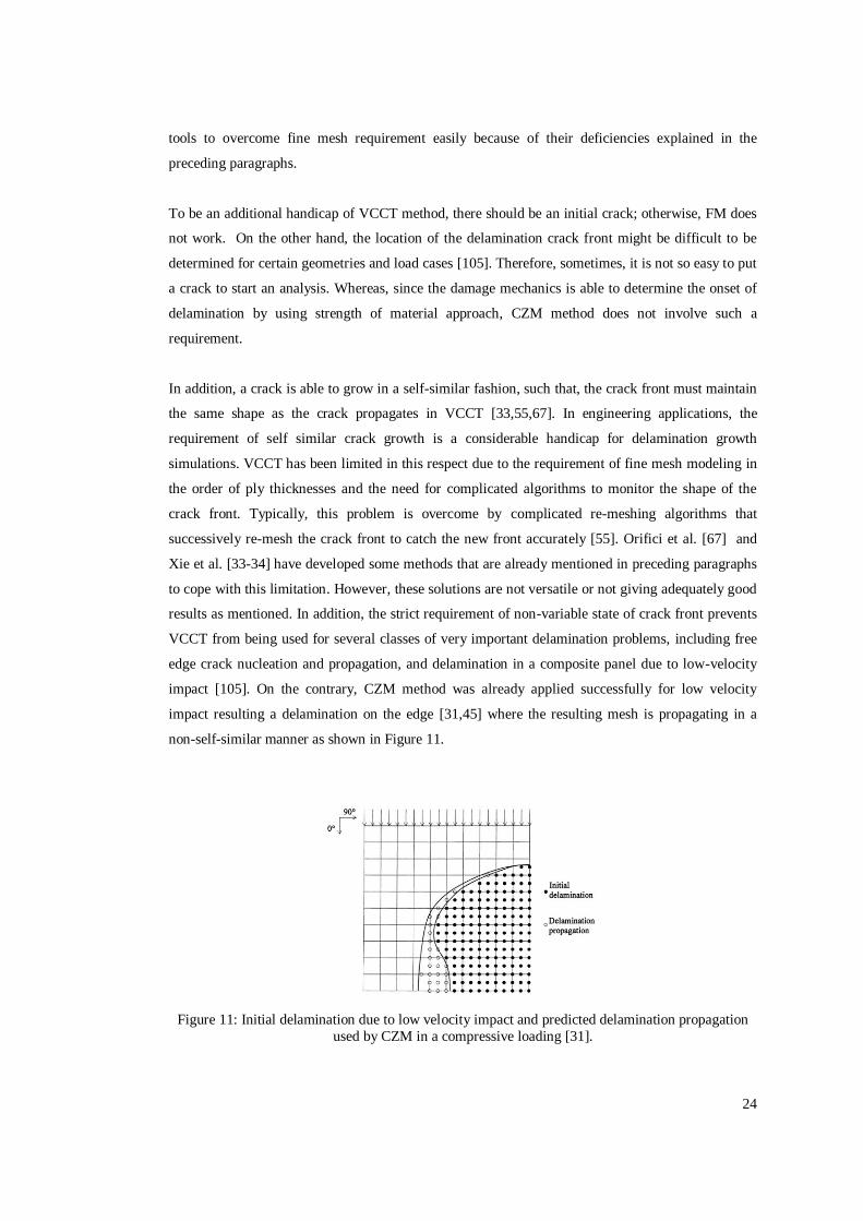
24

tools to overcome fine mesh requirement easily because of their deficiencies explained in the

preceding paragraphs.

To be an additional handicap of VCCT method, there should be an initial crack; otherwise, FM does

not work. On the other hand, the location of the delamination crack front might be difficult to be

determined for certain geometries and load cases [105]. Therefore, sometimes, it is not so easy to put

a crack to start an analysis. Whereas, since the damage mechanics is able to determine the onset of

delamination by using strength of material approach, CZM method does not involve such a

requirement.

In addition, a crack is able to grow in a self-similar fashion, such that, the crack front must maintain

the same shape as the crack propagates in VCCT [33,55,67]. In engineering applications, the

requirement of self similar crack growth is a considerable handicap for delamination growth

simulations. VCCT has been limited in this respect due to the requirement of fine mesh modeling in

the order of ply thicknesses and the need for complicated algorithms to monitor the shape of the

crack front. Typically, this problem is overcome by complicated re-meshing algorithms that

successively re-mesh the crack front to catch the new front accurately [55]. Orifici et al. [67] and

Xie et al. [33-34] have developed some methods that are already mentioned in preceding paragraphs

to cope with this limitation. However, these solutions are not versatile or not giving adequately good

results as mentioned. In addition, the strict requirement of non-variable state of crack front prevents

VCCT from being used for several classes of very important delamination problems, including free

edge crack nucleation and propagation, and delamination in a composite panel due to low-velocity

impact [105]. On the contrary, CZM method was already applied successfully for low velocity

impact resulting a delamination on the edge [31,45] where the resulting mesh is propagating in a

non-self-similar manner as shown in Figure 11.

Figure 11: Initial delamination due to low velocity impact and predicted delamination propagation

used by CZM in a compressive loading [31].

25

A feature of the cohesive method could be stated as a final distinguishing property, which is damage

parameter. Actually, VCCT method can only define the laminate is whether failed or not; just like

―black‖ or ―white‖. On the other hand, CZM method could define the state of delamination over the

damage parameter. For instance, the simulation of the delamination due to the low velocity impact

damage, Batra et al. [45] showed that the damage levels of the crack region is varying as a function

of time as shown Figure 12. One can easily distinguish the regions where the matrix cracking is

emerging, and where the total debonding is occurred. Therefore, even after unloading, intact and

damaged regions can be distinguished.

Figure 12: Fringe plots with the damage parameter evolution [45].

As a summary, although the VCCT method is simpler than the CZM method, the CZM method is

more capable and versatile and even more conservative.

2.3.3 Other Delamination Analysis Methods

In addition to typical FM method and CZM, there are unique and distinguished studies used for the

delamination propagation.

One such proposal is from de Borst [29] and Remmers et al. [78] who offered to bring out the ability

of non similar crack growth for the whole structure. As noticed from Figure 13, the crack can move

in any direction without needing any interface element. In other words, the crack is able to move

―inside‖ the elements, which are used for modeling the intact structure. As a result, a powerful

method has been developed to fully exploit the potential of cohesive-zone models for the arbitrary

crack propagation. Actually, this procedure is referred with a special name called ―XFEM‖ in the

commercial FEA packages [24,64]. The modification here is performed inside the element

formulation of which the details can be found in [29].

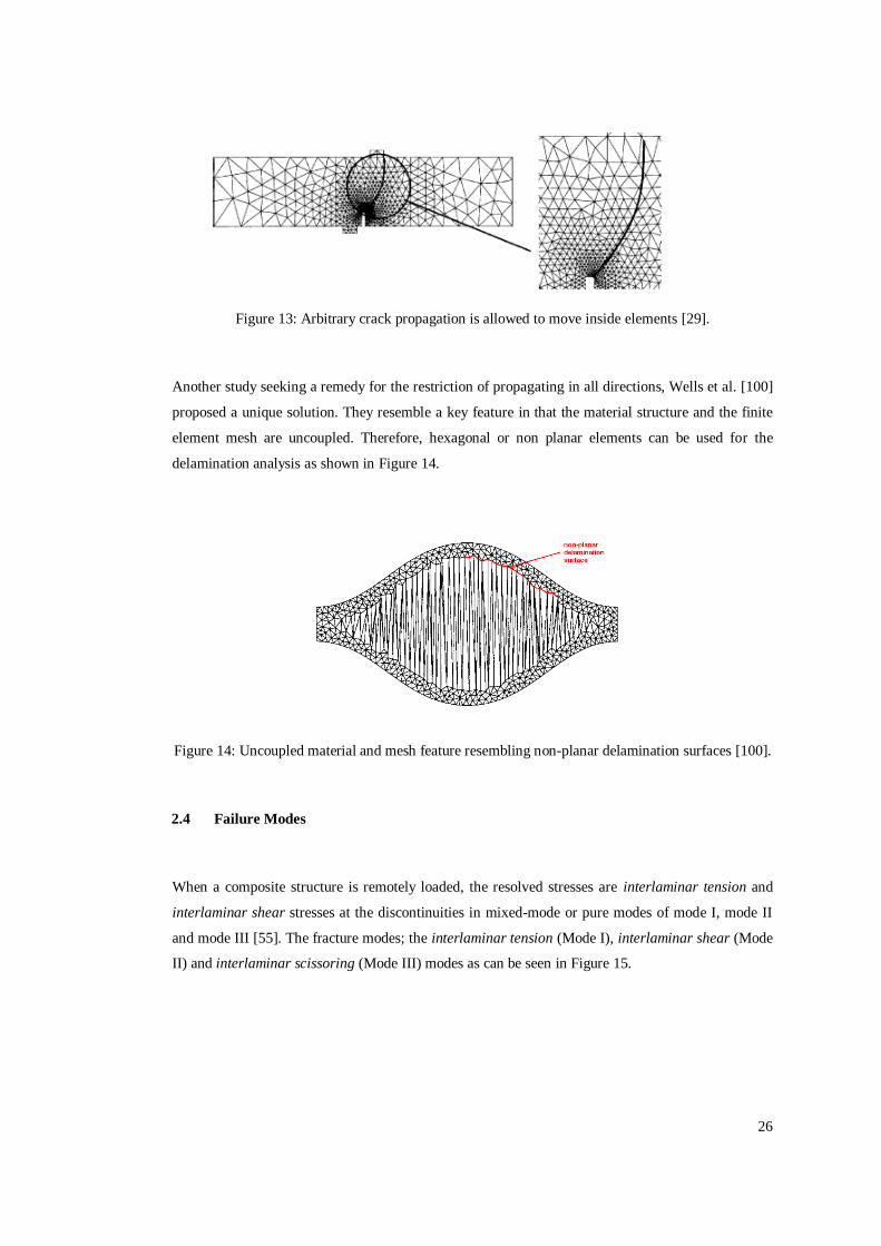
26

Figure 13: Arbitrary crack propagation is allowed to move inside elements [29].

Another study seeking a remedy for the restriction of propagating in all directions, Wells et al. [100]

proposed a unique solution. They resemble a key feature in that the material structure and the finite

element mesh are uncoupled. Therefore, hexagonal or non planar elements can be used for the

delamination analysis as shown in Figure 14.

Figure 14: Uncoupled material and mesh feature resembling non-planar delamination surfaces [100].

2.4 Failure Modes

When a composite structure is remotely loaded, the resolved stresses are interlaminar tension and

interlaminar shear stresses at the discontinuities in mixed-mode or pure modes of mode I, mode II

and mode III [55]. The fracture modes; the interlaminar tension (Mode I), interlaminar shear (Mode

II) and interlaminar scissoring (Mode III) modes as can be seen in Figure 15.

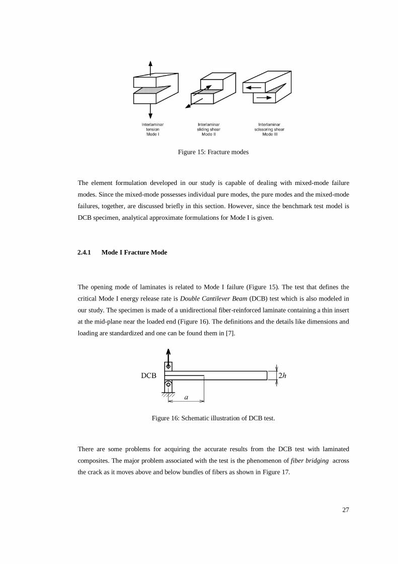
27

Figure 15: Fracture modes

The element formulation developed in our study is capable of dealing with mixed-mode failure

modes. Since the mixed-mode possesses individual pure modes, the pure modes and the mixed-mode

failures, together, are discussed briefly in this section. However, since the benchmark test model is

DCB specimen, analytical approximate formulations for Mode I is given.

2.4.1 Mode I Fracture Mode

The opening mode of laminates is related to Mode I failure (Figure 15). The test that defines the

critical Mode I energy release rate is Double Cantilever Beam (DCB) test which is also modeled in

our study. The specimen is made of a unidirectional fiber-reinforced laminate containing a thin insert

at the mid-plane near the loaded end (Figure 16). The definitions and the details like dimensions and

loading are standardized and one can be found them in [7].

Figure 16: Schematic illustration of DCB test.

There are some problems for acquiring the accurate results from the DCB test with laminated

composites. The major problem associated with the test is the phenomenon of fiber bridging across

the crack as it moves above and below bundles of fibers as shown in Figure 17.

28

Figure 17: Fiber bridging during DCB test [70].

It should be noted that such details are typical characteristic responses of the DCB test, that affect

directly the R-curve as instanced in Figure 18 [13]. One can realize from the below figure that there

are two distinct critical energy release rates (or fracture toughness, GIc); one for initiation and one

for propagation.

Figure 18: R-curve effect on a DCB test of a (0º)24 CFRP laminate [13]

Although DCB test specimens are unidirectional (0º) laminates, it would be convenient to obtain

interlaminar fracture toughness for interfaces between other than 0º plies. Fortunately, it has been

shown that unidirectional composites provide the most conservative values for GIc, such that, higher

values of GIc are obtained for interfaces other than 0º/0º stacking, [13]. Also, a DCB test using arms

with unequal bending stiffness will also promote Mode II loading, [13] A modified DCB specimen

and a new test method designed to overcome these problems, was proposed by Robinson and Song

[84]. Preliminary tests [84] have also resulted in significantly higher values of GIc for

29

multidirectional laminates compared with unidirectional laminates. It is crucial to note that CZM

methodology is same for the multi-directional composites, providing the crack interface surfaces are

in same orientations.

At the crack tip in DCB specimen, the energy release rate across the width decreases closer to the

edges, as shown in Figure 19. One can realize that the plane strain solution is the one at the middle

with a constant value from Figure 19. Actually, such effect seen is due to the anticlastic deformation

[90] which is a three dimensional phenomenon which can be seen only in 3D applications; not in

plane strain problems. Therefore, the anticlastic effect would make the inner sections delaminated

earlier. Figure 19 is directly used for comparing the current energy release rate with the fracture

toughness.

Figure 19: Strain energy release rate across width of DCB specimen at the crack front [90].

The resulting effect for CZM is variation in the process zone where the softening is being shaped as

shown in Figure 20.

30

Figure 20: Evaluation of process zone at crack tip in a DCB test due to anticlastic effects [59].

Although CZM is summarized mainly by means of physical issues, finite element modeling of DCB

test in our study is checked with the analytical approximations. To start the analytical solution, one

can consider one of the arms as a cantilever beam in which the length of initial crack length a0 as

shown in Figure 21.

Δ/2

P

Initial Crack Lenght = ao

h

Figure 21: One of arms is treated as cantilever beam.

From fundamental elastic beam theory, one can find the deflection of the cantilever beam applicable

for a DCB arm;

31

EI

Pa

32

3

0 (3)

Actually, modulus (E) in the above equation is the modulus works ―along‖ the beam, therefore, E =

E11. Moreover, inertia (I) is for simple rectangular cross-section; Bh3/12 where B is the width and h

is the thickness of the arm.

In reality, the clamped surface is being ―rotated‖ during the loading due to the shear deformation of

the assumed ―clamped‖ elastic arm. As a result, the fixed clamped arm assumption would result in

―stiffer‖ results than the real case [77]. Consequently, a ―corrected beam theory‖ is proposed by

Williams et al. [44] who modified the crack length with a correction parameter, χI (Noting the

subscript ―I‖ which is used here is for defining the mode of the correction factor).

IE

haP I

i

11

3

0

3

)(2

(4)

where, the correction parameter, χI can be found both by experimentally or analytically [43]. Our

study takes the analytical solution as follows [44];

2

13

11

123

11G

EI

(5)

where

13

221118.1G

EE

One can observe that the relation between tip load P and tip displacement Δ is linear. Actually, as the

load P increases, the displacement increases linearly.

From the damage mechanics literature, the load can be increased until the cohesive element started to

soften. Until the energy release rate GI reaches the mode I critical energy release rate, GIc. Therefore,

the energy release rate is defined as [77];

32

IBE

haPG

I

I

11

22 )( (6)

Noting that, the initial crack length a0 in Eqn. (6) is replaced by the current crack length ―a‖ due to

the reason that the crack start to vary. As a result, since the ―modified‖ cantilever beam theory and

the energy release rate definition holds throughout the delamination, one can combine Eqns. (5) and

(6) to obtain a unified solution. Since the delamination starts to propagate when GI = GIc, the unified

solution curve after the failure can be written as [77];

2

11

2/3

11

3

)(2

IPE

IGBE Icf (7)

By putting the initial crack length a0 and critical energy release rate GIc inside the Eqn. (6), the tip

force at the crack growth regime becomes;

ha

IBEGP

I

Ic

c

0

11

(8)

Following that, one can easily find the critical tip displacement at the crack growth just by putting

the Pc inside one of the displacement equations above. As a result, the typical response is illustrated

in Figure 22.

33

P

Δ

Δi Δf

GI = GIc

Pc

Δc

Figure 22: Approximate analytical solution for DCB.

2.4.2 Mode II Fracture Mode

Unlike Mode I, there are four distinct types of test for acquiring Mode II fracture toughness, GIIc.

These are (Three Point) End Notched Flexure (ENF), Stabilized End Notched Flexure (SENF), Four

Point End Notched Flexure (4ENF), and End Loaded Split (ELS) tests [27]. Although ENF test

specimen has received the most attention, it has problems associated with unstable crack propagation

for short crack lengths [27]. In fact, the uncertainties are more typical for all of the mode II tests, that

is why; there are many tests suggested with each having a defiance.

The main problems associated with Mode II test are the definition of the type of starter defect, the

definition of crack initiation, the stability of the test, frictional effects on the crack faces and the data

analysis [27]. Actually, since the contact maintained between the delaminated surfaces during the

test, mode II has friction effect throughout the crack [105]. As a reference, the fracture toughness of

Mode II is typically much higher than the one for Mode I. For instance, epoxy matrix composites the

GIIc/GIc ratios typically exceed 2 [27].

34

2.4.3 Mode III Fracture Mode

The delamination can be defined totally only if all subsequent modes are defined. Actually, as to be

seen in the following sections, the main concern for defining the mode test is to obtain the mixed-

mode response of the specimen.

The impact of mode III on delamination is controversial [105]. Just a few studies exist on mode III

failure. According to Donaldson [105], numerical results reveal that the delamination near a notch is

totally driven by mode III. Whereas, Krueger [53] experimentally showed that the effect of Mode III

can be neglected. In our study, since the assumption is plane strain, the mode III effect is

automatically neglected.

There is a candidate testing method for Mode III called Edge Crack Torsion (ECT) test suggested by

Lee [58]. However, the parameter required for the test -the shear modulus G23- needs full

clarification due to the way to be determined [12]. As a result, ECT has not been standardized yet.

2.4.4 Mixed-Mode Fracture

The engineering applications are generally in mixed-mode condition where the loading would not

always be in pure modes. Therefore, the two key points of delamination initiation and delamination

propagation should be investigated. More importantly, the formulations mentioned in this section

are used in the element formulation in our study.

2.4.4.1 Initiation

One of the most widely used criterions for initiation is proposed by Ye [106]. The proposal involves

the pure mode allowable stresses in an interaction that resembles an elliptical behavior. Hence, the

formulation is written as follows [106];

1

222

Ic

I

IIc

II

IIIc

III

t

t

t

t

t

t

(9)

35

where the tIc , tIIc and tIIIc are mode I, mode II and mode III interfacial strengths of the interface.

Similarly, the tI , tII and tIII are mode I, mode II and mode III interfacial tractions. Note that the

operator ‹.› is called Mc-Cauley operator which can be defined as;

2

xxx

(10)

This criterion is called quadratic (or elliptical) criterion that is shown in the Figure 3 with other

criteria. Our study uses this criterion for the delamination onset in order to take into account the

onset of delamination.

2.4.4.2 Propagation

To account for the mixed-mode effect, Reeder and Crews [77] suggested the test of mixed-mode

bending (MMB) which is widely in CZM studies [1,13,16,54,59,71-72] used successfully.

Figure 23: Mixed-Mode Bending (MMB) test [70].

The way for finding the appropriate equations for the MMB test is straightforward. Up to the crack

growth, the MMB is nothing but a superposition of DCB and ENF testing. Therefore, from the

definitions of DCB and ENF, the resulting forces are statically determinate as being formulated in

Figure 24.

36

L a

L

PL

Lc)

2( P

L

Lc)

2(

P

PL

c)(P

L

Lc)(

+=

PL

Lc)

4

3(

c

PL

Lc)

2(

PL

Lc)

4

3( P

L

Lc)

4(

PL

Lc)

4(P

L

Lc)(

DCB ENFMMB = +

Figure 24: DCB and ENF test correlation by superposition feature of MMB (not scaled).

In order to define the amount of the mixture of the pure modes, a ratio should be required. Total

energy release rate GT, the summation of the pure mode energy release rates, is used inside the

definition of the ratio called mixed mode ratio β can be defined as;

IIIIII

II

T

II

GGG

G

G

G

(11)

A typical result of mixed mode interaction for an epoxy matrix carbon fiber composite is shown in

Figure 25. The first point in the curve is GII/GT = 0, showing that the only contribution is by mode I.

Therefore, DCB test can be used to locate this point. Conversely, there is pure mode II if the GII/GT =

1; hence, ENF test is adequate. On the other hand, successive MMB tests are required for finding the

mid-points. So as to cover the curve, different GII/GT is selected and tested by MMB. An example for

a typical result is illustrated in Figure 25 for an epoxy/graphite composite.

37

Figure 25: Mixed-Mode and mode I, II failure criteria for an epoxy/graphite composite [95].

Benzeggah and Kenane [9] suggested a failure criterion by curve fitting for Gc vs β curve (Figure

25) as follows;

))((T

IIIcIIcIcc

G

GGGGG

(12)

where the factor η is found by curve fitting. Benzeggah and Kenane (BK) criterion is taken as a

failure criterion for CZM analysis successfully; for instance, by Unified Mode Approach [13,105].

38

Figure 26: Factor of η in Benzeggah and Kenane criterion, α for power law criterion and

corresponding fracture toughness values for various composites [12].

Nevertheless, Eqn. (12) cannot be applied easily for all engineering applications, because of the

requirement for experimental data to find the factor η. Therefore, a more robust failure criterion was

suggested and used effectively, which is called power law [2,59,72];

1IIc

II

Ic

I

G

G

G

G

(13)

where for most of the carbon/epoxy composites, the mixed-mode data can be accurately represented

using 1 ≤ α ≤ 2 [15,71]. For instance, PEEK matrix composites are best fitted with α = 1 [12]. It

should be noted here that Separated Mode Approach uses power law criterion since the failure

criterion is represented only by pure mode energy release rate values.

One may remark that the above mixed-mode propagation criteria do not involve GIIIc. This is due to

the facts that are mentioned in the mode III section. Consequently, it is generally suggested to use

propagation equations by replacing GII terms with shear energy release rate definition such that

Gshear = GII + GIII [12]. Since our analysis is two dimensional with plane strain assumption, there is

no Mode III energy release rate; therefore, this automatically yields; Gshear = GII.

Finally, to show the whole picture, the tip load vs. displacement curves and the corresponding

critical loads for delamination crack propagation can be compared from Figure 27.

39

Figure 27: Various mode tests for AS4/PEEK carbon fiber unidirectional composite [12]

40

CHAPTER 3

3 COHESIVE ZONE METHOD DELAMINATION ANALYSIS

3.1 Cohesive Zone Model

The cohesive zone approach can be explained on a detail view of the crack tip. The crack has a

process zone acting as a transition region between traction free and the linear elastic region of the

bulk material [8]. This region has a different non-linear profile; named by Barenblatt [8] as outer

region whereas the traction free part it is named as inner region.

The physical phenomena behind the process zone was first proposed for concrete materials as

bridging due to second phase particles and away from bridging, micro-cracking were responsible

[48]. This can be characterized as micro structural linkage units may be identified with cohesive

bond in brittle solids, ductile filaments in plastic solids, transverse molecular chains in polymers [5].

For composites, however, load-bearing fibers, voiding and crazing are the physical phenomena

resulting in such a process zone [5].

Intact regionTraction free crack Process Zone

Broken bonds

Cohesive

Forces

(a) (b)

Figure 28: (a) Bonding and de-bonding actions for the process zone (b) Top view of inner and outer

regions

41

In Figure28a, it can be realized that the process zone is illustrated by set of ―springs‖ so as to imply

the existence of cohesive forces which result in a unique traction profile at the crack edge. Also, the

edge of the crack is drawn like sharp tip of a water drop to reveal that the cohesive effect is dominant

in the cohesive zone only. In fact, the springs are considered as a continuum of cohesive forces in

Continuum Cohesive Zone Method (CCZM) whereas they are discretely taken into account in

Discrete Cohesive Zone Method (DCZM), pioneered by Xie and Waas [32]. The theory behind both

approaches are identical, just the methodology in element modeling is different. However, both cases

are valid, only if the process zone is much smaller than the crack [6,8]. In our study, the most

generally used method; Continuum Cohesive Zone Method is used because of the interface element

type selected.

The application of the cohesive zone method is directly based on which of the cohesive models

being used. CZM relates tractions to displacement jumps at an interface where a crack may occur

[42]. In other words, the models contribute traction (or stress)-displacement profiles dealing with

specific materials and interfaces. The first cohesive stress model suggested by Dugdale [36] was

using constant stress profile for dealing with plastic materials as shown in Figure 29a. However, the

proposal gives full plastic behavior which could not yield correct results for composite materials.

The most frequently and successfully used model is the one called bilinear model proposed by Mi et

al. [59] (Figure 29b). The bilinear model gives accurate results for composite materials and that is

why this model is used in our study.

(a) (b)

Figure 29: (a) Dugdale model [36] in cohesive zone (b) Cohesive zone stress distribution by Mi et al.

[59].

42

The application of cohesive model is performed by finite element analysis in which the candidate

delamination surfaces are modeled by interface elements (Figure 30) obeying cohesive zone

constitutive relationship. As understood from the name ―interface‖, the elements are located between

the adjacent plies where the delamination occurs.

Figure 30: FE model and 3D interface elements in a DCB test specimen [43].

In fact, the interface elements are supposed to be in zero or near-to-zero thicknesses because they are

located in the interfaces without affecting the real thickness, or simply the whole part. Otherwise, the

interface element can increase the actual thickness of the specimen; hence, the global response can

be incorrect. This is the reason why the constitutive relations depend on displacements, not strains.

Otherwise, one can come up with extremely sensitive strains which may result in numerical

instabilities for FE solvers. Moreover, as can be seen in the following paragraphs, FE solver would

give aspect ratio errors [61] because of the element height over element width ratio become near to

zero.

The displacements in CZM are relative displacements; δ, as shown in Figure 31 in which the two

surfaces represent the adjacent delamination surfaces. In other words, the lower and upper surfaces

are adjacent laminas in our study. The relative displacement is between the ―top‖ and the ―bottom‖

surfaces in the interface continuum. Later on, this definition will be presented in more detail.

Figure 31: Cohesive element relative displacement definition and separation of the surfaces.

43

After the above fundamental definitions, it is better to return to cohesive zone models and

corresponding constitutive relationships. A typical constitutive relationship for composite

delamination analysis is the one used in the pioneering work of Needleman [66] shown in Figure 32.

Recalling that, there are pure modes (Mode I, Mode II, and Mode III) being related to the

engineering problems. Thus, the normal traction versus opening displacement curve shown in Figure

32a is the Mode I response, whereas, the shear traction versus tangential displacement curve shown

in Figure 32b, is the Mode II or Mode III.

Openning

Traction

Openning

Displacement

0

0

Tangent

Traction

Sliding

Displacement

0

0

(a) (b)

Figure 32: Needleman's traction-displacement constitutive model, [66] (a) for Mode I and (b) for

Mode II (or Mode III).

It can be easily seen from Figure 32 that the shear and opening mode responses have a similar

behavior, yet with a different behavior at negative displacement. For mode I, any negative relative

displacement corresponds to interpenetration of delamination surfaces which cannot be allowed [72].

Therefore, quite a stiff resistance would emerge for preventing the interpenetration of the

delamination surfaces. On the other hand, for Mode II and Mode III, the negative relative

displacement is nothing but a directional situation for the deformation. Consequently, whether the

displacement is negative or not, the response of the cohesion zone would be the same.

In addition to Needleman’s study, there are various constitutive formulations proposed for

delamination analysis; linear elastic, linear softening, linear elastic-progressive softening and linear

elastic-regressive softening [27] as summarized in Figure 33.

44

Figure 33: Various traction-displacement interface constitutive relations [27]

From Figure 33, it can be revealed that all of the constitutive relations have similar behaviors. This is

due to the fact that the interface elements behave in three unique regions; [1,13,16,59,95-96];

Intact region,

Softening region,

Failed region.

They are all shown in Figure 34, illustrating on the bilinear relationship.

Intact Softening Failed

tc

δ o δ c δ

t

Figure 34: Characteristics of constitutive relations (bilinear relationship).

Intact region is dedicated for the ideal bulk material representation, that is, the undamaged part. The

intact region goes up to the point (δo,tc) where delamination onset occurs. This is the point where

chemical bonds of the intact materials start to be broken, in other words, the cohesive phenomenon

starts. Therefore, the maximum traction tc is the interfacial strength defining the onset.

45

There remains only the delamination onset δo which is not related to any phenomenon. Actually, this

parameter has nothing to do with CZM. The implantation of the method yields non-zero

delamination onset displacement does, because of the requirement of initial tangent stiffness matrix.

The slope of the curve in intact region is called penalty stiffness, E0 being selected as high as

possible for giving accurate results while avoiding excessive values causing convergence problems

[96]. More specifically, using high penalty stiffness would result in high stresses in accordance with

the singularity which is found in the traction profile at a sharp crack tip in a LEFM model for having

a sufficiently accurate pre-crack behavior [72]. As going to be discussed in our study, this parameter

is very important for CZM.

After delamination onset, the softening of the interface occurs due to the cohesive effects like fiber

bridging, crazing and microvoiding [13,105], which are pointing the phenomenon of cohesive

effects. Softening region is the one between delamination onset displacement δo and the critical

displacement relating to the total failure, δc in term of the constitutive relationship. Moreover, the

softening region is the problematic phase responsible for the sharp-snap backs that would yield

convergence problems, [2,59].

The requirement for a softening region emerges due to damage mechanics approach being used for

deriving the constitutive behaviors [1,95]. The details of damage mechanics derivation shall not be

given here, since it is discussed extensively in [1,95]. Yet, damage mechanics derivation results in

the traction versus displacement profile that is given as follows [1];

0)1( Edt (14)

where the “d” is the damage term to be defined analytically in the next chapter. One can understand

from Eqn. (14) that the line equation of “(1 - d)E0” shows a declining behavior as the damage term

increases from no damage value of 0 to fully damaged value of 1. This reveals a theoretical cohesive

zone as shown in Figure 35.

46

t

δ

d = 0

d = 1

Figure 35: Theoretical cohesive zone constitutive relationship with ―infinite‖ penalty stiffness.

For the last phase, when the critical displacement, δc exceeded (or damage is fully attained with

d=1), full delamination happens; or in words the interface element is fully failed. After this point, the

cohesive elements would behave as a traction free crack. It should be noticed that, the existing

phenomenon other than cohesive forces like interpenetration prevention for Mode I or frictional

effects for Mode II and Mode III are still active. Actually, this feature has nothing to do with

cohesive methodology; however, it is used for the sake of modeling ―real‖ interfaces.

3.1.1 Definition of Cohesive Zone Length

The boundary of cohesive zone was implied in the previous paragraphs as the distance from the

maximum attained traction to the zero traction. It is shown as Γ, defining the cohesive zone as the

detailed view given on a DCB specimen in Figure 36. Hence, the region bounded by the points 2 to 4

defines the softening of the interface; the cohesive zone.

47

Figure 36: Cohesive zone in the vicinity of crack and bi-linear constitutive relationship. (Not to

scale)

Actually, the size of cohesive zone is referred as cohesive zone length in literature. The word

―length‖ is used since the thickness of the zone is quite small and therefore it can be neglected.

Turon et al. [96] studied the length of cohesive zone extensively. It is pointed that [96] there are

many analytical cohesive zone length approximations variable from specimen to specimen. It is also

stated that the main characteristics of all proposed length approximations have the same structure

that is given as [96];

222)(

)(c

ccz

t

GEMl

(15)

Where different M values are given in Table 1;

Table 1: Different M values for plane stress approximation in literature [96]

Proposed by; M

Hui et al. 0.21

Irwin 0.31

Dugdale and Barenblatt 0.40

Rice, Falk et al. 0.88

Hillerborg et al. 1.00

Remaking, the above length approximations are for plane stress condition; unlikely used for our

study. Also, the original version of Eqn. (15) uses isotropic modulus (E) instead of transverse

48

modulus; (i.e; E22 = E). Note that, Turon et al. [96] obtained best results with the approximation of

Rice. This result is going to be checked in our analysis also although it is for plane stress.

On the other hand, Harper and Hallet [43] once remarked that the theoretical cohesive zone length

formulations in literature and the one obtained by FEM are different. Therefore, the exact matching

for the above formulations with FEM results cannot be met.

The cohesive zone length is directly related to the convergence issue that is the most crucial point for

the CZM applications. The most predominant convergence effective criterion is the mesh density in

the cohesive zone [15-16,71-72,96]. Turon et al. [96] suggested that the minimum number of

elements required for reaching converged solutions should be more than two elements. Therefore,

the resulting element length can be given as;

3

cze

ll

(16)

Where le is the length of individual interface element located inside the cohesive zone. As a note

here, there is a trick usually performed by the researchers, and also done in some cases in our study.

It is to increase the cohesive zone length so as to benefit convergence rate [2]. Actually, the trick is

activated by artificially lowering interfacial strength in Eqn. (15), that increases the cohesive zone

length, and at the same time the number of interface elements staying inside the zone. However, this

artificial modification would not yield accurate results if the interfacial strength was decreased

excessively [43]. This phenomenon is also revisited in our bench mark test model.

As a summary, the whole process of damage advancement can be illustrated in Figure 37. It can be

seen that, there are two elements initially representing the cohesive zone. When the critical tip

displacement attained, the cohesive zone is ―hatched‖ and started o get expand to the right. One may

reveal that some elements may reach to the maximum traction (tc) and start to be softened, before the

maximum tip force is attained. Actually, the point, where the maximum tip load attained, is the

location where a mature cohesive zone formed.

49

Figure 37: Cohesive zone evolution as tip load increases for a DCB test model [43]. (LCZ: The Cohesive Zone Length)

3.1.2 Griffith’s Theory in CZM

Although the original derivation should be the damage mechanics, the cohesive zone formulation is

also identical to Griffith’s theory of fracture [40]. It should be noticed that the use of Griffith’s

theory is not fully correct in terms of the assumptions it requires. However, for the sake of simplicity

and the equivalence of the resulting equations, Griffith’s theory is used in our study to finalize the

CZM formulation.

Now, if one considers the J-integral proposed by Rice on the boundary Γ [80];

)( dsx

utwdyJ

(17)

50

where Γ is any contour surrounding the notch tip, u is the displacement vector, t is the traction vector

defined accordingly to the outward normal along Γ, and w is the strain energy density. From the

constitutive relation shown in Figure 36;

))(( dxx

wdyJ

(18)

By neglecting the thickness of the cohesive zone, it can be taken into account that dy = 0 for the

selected integral path;

00)())(())(( ddxd

dx

ddx

xJ

(19)

Under the assumptions of self similar crack growth and small cohesive zone comparing with the

crack length, one may use the energy release rate definition as, [80];

Ga

J

(20)

Therefore, from Eqn.(19) and Eqn. (20);

0)( dG

(21)

Considering the final crack displacement of the critical displacement, δc;

c

dGc0

)(

(22)

Meaning that the area under the constitutive relationship is equal to the critical energy release rate,

Gc. As a result, since the remaining unknown parameter, the critical displacement, δc is found, the

whole bilinear constitutive relation is now attainable.

51

3.2 Mixed-Mode Cohesive Zone Model Derivation

Up to now, we considered the pure mode constitutive behaviors and their fundamentals. However,

the response of delamination would not be straightforward in the mixed-mode loading. Just like in

the critical energy release rate, a study for the mixed-mode cohesive constitutive relationship is

compulsory. Notably, although there would be no benchmark test like MMB in our study, the

elements would have full capability for dealing with mixed-mode loading, and therefore, the mixed-

mode formulations are going to be derived.

Now, consider a 3D interface element shown in Figure 38. The total relative displacement vector δ

can be defined in terms of local coordinate system (I,2,3) displacements; δI, δ2 and δ3 as;

2

3

2

2

2

I (23)

It can be seen that the subscript for opening displacement is taken with the character ―I” whereas the

numeric subscripts of 2 and 3 are used for the Mode II and Mode III, respectively. This is due to the

fact that, the orthogonal displacement component corresponds to the opening mode I. On the other

hand, the others are contributing the shearing displacement together as discussed before.

Figure 38: Pure mode displacements in an interface element.

Repeating here, Mode-III has very little effect; therefore, it is convenient to consider the

displacements δ2 and δ3 as one as the shear mode. As a result, the contribution of Mode III is going

to be neglected for the rest of this study.

The shear displacement δshear can be written as, [71],

52

2

3

2

2shear (24)

Then, Eqn. (23) becomes;

22

shearI

Now, consider the opening mode and the shearing mode constitutive bilinear relations given in

Figure 48;

GIc

tIc

δIc δ

t

GIIc

tIIc

δIIcδ

t

(a) (b)

Figure 39: Pure mode bilinear constitutive relationship.

For a mixed mode ratio of β = 0 the pure Mode I behavior on Figure 39a is adequate because the

maximum interfacial strength and the critical energy release rate in Mode I is known from DCB

tests. Similarly, for β = 1, the pure Mode II behavior on Figure 39b is adequate to proceed the

analysis due to the Mode II test has already been specified. However, this is not the case for the

mixed-mode, because the mixed-mode ratio varies as the loading advances. The failure criterion

would be varying due to the interfacial strength is being changing due to quadratic criterion and the

critical energy release rate is found by either the BK-criterion or power law. Finally, the resulting

constitutive behavior should be the one shown in Figure 40.

53

Figure 40: Constitutive relationship for Mixed-Mode delamination

In Figure 40, it can be seen that there are superscripts ―M‖ used for the mixed-mode extremities for

the corresponding parameter in pure mode planes. Actually, there are two extremities; one for the

pure modes and the other for the mixed mode. The reflections of the mixed mode ratio constitutive

relation (the triangle at the middle) on the pure mode planes are to lower the maximum pure mode

energy release rates (i.e.; GIc > GIcM and GIIc > GIIc

M) and the pure mode maximum of the tractions

(i.e.; tIc > tIcM and tIIc > tIIc

M) and the displacements (i.e.; δIc > δIcM and δIIc > δIIc

M similarly, δIo > δIoM

and δIIo > δIIoM). As a result, the all of the constituents for deriving the appropriate constitutive

relationship can be performed by investigating Figure 40.

Many authors [16,27,43,59,71,96] pointed out that by maintaining the critical energy release rate,

there would be no considerable difference among the all constitutive relationship results, even for

artificially adjusting the interfacial strength for better convergence rates. On the other hand, Yang

54

and Cox [105] suggested using accurate constitutive relations for highly mixed-mode loading.

Hence, the ―rigidity‖ such a figure of Figure 40 is controversial.

3.2.1 CZM Constitutive Formulations for Mixed-Mode Failure

All of the approaches in literature start with fundamental formulations of the pure mode failures. In

intact region, the penalty stiffness matrix generally has a pre-defined value avoiding numerical

instabilities [96]; thus, the pure mode delamination onset displacement is the one found directly from

the slope of the penalty stiffness as follows [1,12,71];

IIIiE

ticio ,,

0 (25)

The subscript ―i‖ is addressing pure modes, and E0 is the penalty stiffness which is going to be

distinguished for Mode I and Mode II by Separated Mode Approach [1]. On the other hand, for

Unified Mode Approach [12], the penalty stiffness values for each pure mode are identical. Actually,

the difference of the two starts from the definition for the penalty stiffness concept.

From the area of the triangle in Figure 34, the pure mode critical displacement can be found easily,

[1,12,71];

IIIiE

G

io

Icic ,,

0

2

(26)

After that point, the pure constitutive relationship on mode planes of Figure 40 can be drawn.

Afterwards, the mixed-mode approaches could be defined according to both formulations.

The basis for damage evolution is the total relative displacement, δ as suggested by Allix and

Corigliano [3], Camanho et al. [12] and Pinho et al.[71]. Therefore, firstly by revisiting Eqn. (23),

the interpenetration phenomenon in opening mode can be handled as follows;

55

222

3

2

2

2

shearII (27)

where the δI is defined in Mc-Cauley brackets Eqn. (10) so as to remove any ―closing‖ displacement

from the total displacement parameter. As to be seen from the following paragraphs, the case for

negative Mode I displacement is considered separately and named as interpenetration.

For mixed-mode ratio, β, Figure 40 shows that it is equal to the tangent θ;

I

shear)tan(

(28)

Referring to Figure 40, one may find the mixed-mode onset displacement by putting the onset

displacement given in Eqn. (23) into the mixed-mode quadratic criterion in Eqn.(9);

0

0)(

122

2

0

IIIo

I

IoIIo

IoIIo

(29)

Remaking that, the negative displacement of Mode I is referring to interpenetration, where the mode

I diminishes.

Now, from the angle of the mixed-mode, one can find δioM and δic

M ( i = I,II ) as follows;

)cos(0

M

Io

)sin(0

M

IIo

(30)

)cos(c

M

Ic

)sin(c

M

IIc

(31)

Actually, we may assume the same penalty stiffness values for Mode I and Mode II. As a result, the

energy release rate values can be written as;

56

,2

0)(cos2 EG oc

I

2

0)(sin2 EG oc

II

(32)

By inserting Eqn. (32) in the B-K criterion given in Eqn. (12), the critical displacement value for the

mixed-mode van be found;

0

01

)(0

22

2

IIIc

IIcIIcIc

o

c

GGGE

(33)

Similarly, for the power law criterion;

0

01

0

)1(2/1

22

IIIc

I

IIcIco

c

GGE

(34)

Just as done in the derivation of delamination onset displacement, the resulting critical displacement

would be the failure displacement for pure shear due to the removal of the closing displacements.

Upto point, all of the constituents shown in Figure 40 have been determined. However, the

requirements for embedding the formulation into the interface element are traction and tangent

stiffness matrix of an interface element. However, before going through the details of them, the

irreversibility concept of the cohesive zone should be pointed out.

As seen in Figure 41, assume that the loading had started from point 0 and goes to point 3 through

point 2 where the delamination emerges and following it the softening occurs. Afterwards, if the

element is unloaded, the curve goes directly to point 0 because the cohesive zone is not fully elastic.

Assume that the element is going to be loaded again, then the arrow in Figure 41 would be reversed

57

and the shaded area is never going to be used again. Therefore, the process is irreversible since some

of the energy release rate has been ―consumed‖ during the first loading.

Figure 41: Constitutive relationship with unloading reveals irreversibility.

The definition of time should be considered in order take the irreversibility into account as follows;

)(max)(max

tt

(35)

Notably, since the finite element analysis solver is an implicit one, the time parameter in Eqn. (35)

is the iterations considering the quasi-static analysis.

Now, recalling the damage mechanics formulation of the cohesive zone given in Eqn. (14), the

damage term ―d‖ can be defined just by considering the geometrical relations in Figure 41;

)(1

)(

)(

)(0

max

max

max

max

max

FAILED

INTACT

d

c

co

oc

oc

o

(36)

Therefore, by putting the damage term of Eqn. (36) into Eqn. (14), it would give the constitutive

relationship. However, it is better to use typical representation for the element formulation [107];

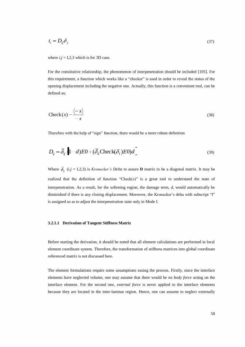
58

jiji Dt

(37)

where i,j = I,2,3 which is for 3D case.

For the constitutive relationship, the phenomenon of interpenetration should be included [105]. For

this requirement, a function which works like a ―checker‖ is used in order to reveal the status of the

opening displacement including the negative one. Actually, this function is a convenient tool, can be

defined as;

x

xx)(Check

(38)

Therefore with the help of ―sign‖ function, there would be a more robust definition

dEEdD IiIijij )0)(Check(0)1(

(39)

Where ij

(i,j = I,2,3) is Kronecker‟s Delta to assure D matrix to be a diagonal matrix. It may be

realized that the definition of function ―Check(x)‖ is a great tool to understand the state of

interpenetration. As a result, for the softening region, the damage term, d, would automatically be

diminished if there is any closing displacement. Moreover, the Kronecker’s delta with subscript ―I‖

is assigned so as to adjust the interpenetration state only in Mode I.

3.2.1.1 Derivation of Tangent Stiffness Matrix

Before starting the derivation, it should be noted that all element calculations are performed in local

element coordinate system. Therefore, the transformation of stiffness matrices into global coordinate

referenced matrix is not discussed here.

The element formulations require some assumptions easing the process. Firstly, since the interface

elements have neglected volume, one may assume that there would be no body force acting on the

interface element. For the second one, external force is never applied to the interface elements

because they are located in the inter-laminar region. Hence, one can assume to neglect externally

59

applied forces on the element. As a result, the only internal force R vector can be found from the

principle of virtual work [107] as follows;

V

T dVtBR

(40)

Where B matrix is nodal displacement-to-relative displacement matrix, t is the traction vector and V

is the volume of the interface element. B matrix is a key matrix that is directly relating the relative

displacement vector δ to the nodal displacement p as follows;

Bpδ

(41)

It is vital to note that Eqn. (41) involves the rotated or transformed B matrix that is explained in

chapter 5.1.2. Note that, the relative displacement vector δ in Eqn.(41) should not be confused with

the total relative displacement vector δ given in Eqn.(23) which is the magnitude of the vector δ.

By inserting Eqns. (37) and (41) in Eqn. (40), it follows that;

V

T dVDδBR

(42)

The tangent stiffness matrix can be found from the derivative of the internal force [107] as

s

t

o

tt KKδp

DBDBB

p

RK

V

T

V

T dVdV

(43)

where

V

T dVDBBKo

t

V

T dVδp

DBK

s

t

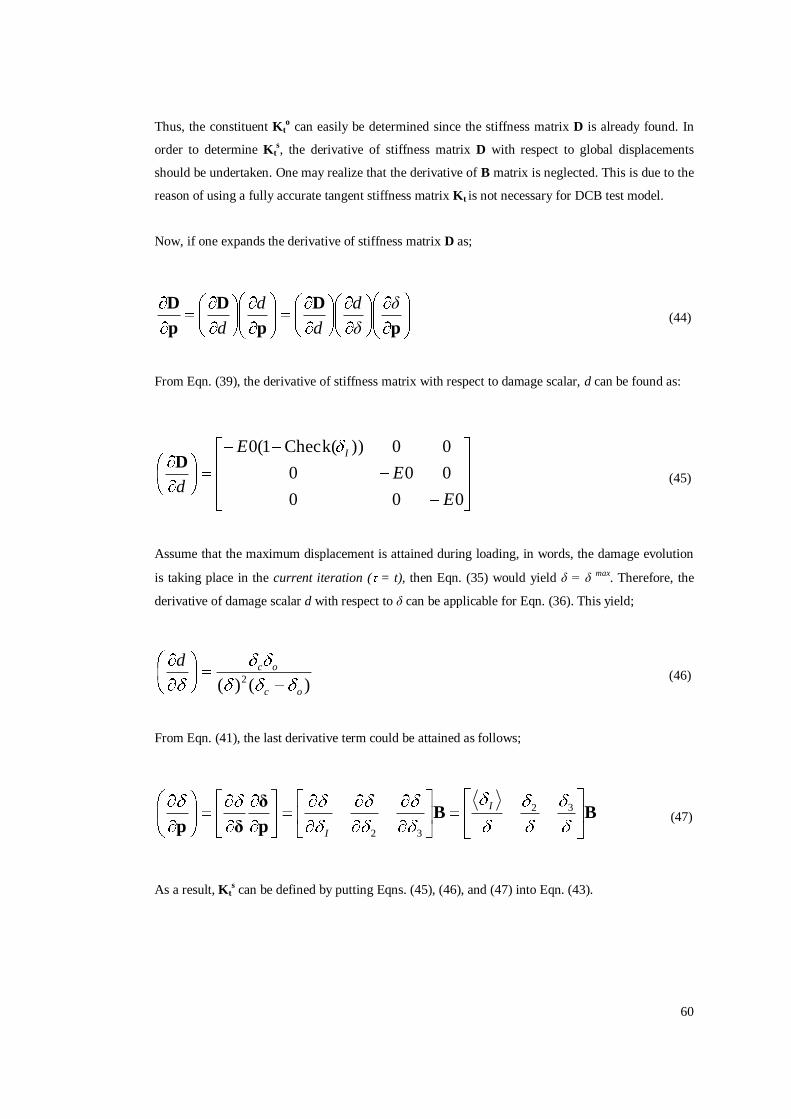
60

Thus, the constituent Kto can easily be determined since the stiffness matrix D is already found. In

order to determine Kts, the derivative of stiffness matrix D with respect to global displacements

should be undertaken. One may realize that the derivative of B matrix is neglected. This is due to the

reason of using a fully accurate tangent stiffness matrix Kt is not necessary for DCB test model.

Now, if one expands the derivative of stiffness matrix D as;

p

D

p

D

p

D δ

δ

d

d

d

d (44)

From Eqn. (39), the derivative of stiffness matrix with respect to damage scalar, d can be found as:

000

000

00))Check(1(0

E

E

E

d

ID

(45)

Assume that the maximum displacement is attained during loading, in words, the damage evolution

is taking place in the current iteration ( = t), then Eqn. (35) would yield δ = δ max. Therefore, the

derivative of damage scalar d with respect to δ can be applicable for Eqn. (36). This yield;

)()( 2

oc

ocd

(46)

From Eqn. (41), the last derivative term could be attained as follows;

BBp

δ

δp

32

32

I

I

(47)

As a result, Kts can be defined by putting Eqns. (45), (46), and (47) into Eqn. (43).

61

Inte

rpen

etr

ati

on

Pre

ven

tio

n

Unload/R

eload

t

δ(1-d)E0

E0

Figure 42: Constitutive relation minimum features.

Now, it is time to grant the tangent stiffness matrix in terms of loading, unloading, damaging and the

interpenetration prevention features as shown in Figure 42. As a summary;

1. Intact Region: δmax ≤ δo and at any time the response is similar to a typical linear law;

V

T dV

E

E

E

BBK t

000

000

000

(48)

2. Softening Region: δo < δmax ≤ δc, the tangent stiffness is varying from secant to the tangent

one. Therefore, the formulation should be divided into two.

a. Unloading/Reloading with no damage evolution; δ < δmax

V

I

T dV

Ed

Ed

CheckdEEd

BBKKo

tt

0)1(00

00)1(0

00)(00)1(

(49)

b. Damage evolution (loading state); δ = δmax

62

s

t

o

tt KKK

(50)

where Kts can be written explicitly.

V

T

I

I

I

T

oc

oc dV

E

E

CheckE

BBKs

t

3

2

3

2

2

000

000

00))(1(0

)()(

T

his yields;

V

II

II

IIIIIII

oc

ocT dV

Check

Check

CheckCheckCheckE

BBKs

t

33233

32222

32

3

)(1(

)(1(

)(1()(1())(1(

)()(

0

3. Failed Region: δmax > δc, only the interpenetration can be provided to the system.

V

I

T dV

ECheck

BBK t

000

000

000)(

(51)

63

CHAPTER 4

4 CONVERGENCE ISSUE AND ARC-LENGTH METHOD

4.1 Convergence Issue

Apparently, the most challenging feature of the Cohesive Element Method is the convergence issue.

Therefore, this section is dedicated for the discussion of numerical solution and the properties of

CZM spawning divergences. Importantly, the discussed items in this section are to be checked and

used in our study.

4.1.1 “Trouble” in CZM and Literature Survey

The local softening behavior of the interface elements results in a global softening response of the

structure [2]. As a result, this causes ―hard-to-catch‖ equilibrium points. Naming, severe snap-back

and snap-through behaviors are observed [21-22]. In addition to the severe nonlinearities, there are

also oscillations in the equilibrium path, because of the positive slope of the total potential energy

[22]. In addition to the softening, the high penalty stiffness requirement overshoots the equilibrium

[12] and even causes numerical instabilities. Consequently, CZM requires considerable study in

numerical solution scheme.

The structural responses like snap-through, snap-back, brittle collapse and ductile collapse are

illustrated in Figure 43. Widely used numerical solution methods like Full or Modified Newton-

Raphson (N-R) methods applies ―fixed‖ loading during iterations. Thus, none of them have ability to

deal with problems involving snap-through, snap-back, brittle collapse and ductile collapse behavior

[22,61].

64

A

B

C

Lo

ad

Displacement

Lo

ad

Displacement

A

B

CDynamic

Lo

ad

Displacement

A

B

Y

L

oa

d

Displacement

A B

Figure 43: (a) Snap Back (b) Snap Through (c) Brittle Collapse (d) Ductile Collapse cases [22].

For a deeper understanding of these discrepancies, it would better to consider each case individually

from Figure 43. Initially, all cases start with point A which is last converged position. For Figure

43a, snap-back behavior is shown where a displacement controlled, with non flexible iterative

method, like N-R is only able to catch point C while missing the intermediate equilibrium points like

point B, staying outside the constant displacement shown as dashed line. Similarly, in the case of

Figure 43b, any non-flexible load controlled method could only catch point C instead of point B for a

snap-through case. For the cases in Figure 43c and Figure 43d, constant load line is not able to catch

the equilibrium points located on the right hand side. Even for the top points of the curves, tangent

stiffness matrix diminishes. Consequently, this yield ―goes to infinity‖ situations, or at best,

overshooting the points where the convergence is impossible. Therefore, as to be discussed in the

following paragraphs, a ―constraint equation‖ should be embedded into governing equations to move

around such problematic points. This is accurately done by Arc-Length Method, which circumvents

problematic cases with great flexibility to catch sharp snap-back and snap-through cases [22].

In the current study, the solution is performed by a commercial non-linear solver MSC MARC

2005r3 [64]. The solution in our study is performed by quasi-static loading in which the external

loads and the prescribed displacements are supposed to be continuously adjusting themselves so as

to be in the state of equilibriums progressively in each increment [61]. However, one could claim

that in reality, loads do not adjust themselves to gain ―flexibility‖, even if they are applied quasi-

statically [20]. One would also suggest that such limit points might induce dynamic phenomena, like

(b)

(c) (d)

(a)

65

―dynamic snaps‖ from one to another stable branch of the equilibrium path, or with a final structural

collapse just like N-R does as shown in Figure 43b. This method is being used for cohesive element

method, which is called hybrid static/dynamic method [20]. Just for a reference, this procedure is

also explained hereafter briefly since it shows a candidate CZM solver for the future.

The methodology of hybrid method is for ―jumping‖ over snap through areas by appending

dynamics. In words, the procedure goes up to limit points by using standard methods. Afterwards,

when a current stiffness parameter reaches a critical point –that depicts the critical point is inside the

vicinity – then the perturbation load is increased monotonically while the procedure transits from

statics to dynamics with a prescribed initial velocity [20]. This procedure is illustrated in Figure 44.

Figure 44: Hybrid static/dynamic solution procedure on a snap-through region [20].

As understood from the original name, the hybrid method involves both dynamic and static solution

phases. The dynamic solution procedure could be explicit or implicit [20]. It is worth noting that an

explicit approach within a quasi-static analysis would have the advantage compared to the implicit

methods, in the way of the equilibrium not having to be rigorously satisfied at each increment [2].

Yet, specific to the cases where small dynamic regions with high nonlinearities, the hybrid method is

a promising method for the future studies.

4.1.2 Coping with Convergence Problem

There are suggestions to enhance the convergence rate of CZM. In this section, they are mentioned

in the way that literature takes them into account. Reminding that, these suggestions are called as

artificial modifications and revisited in our study.

66

The numerical solution of a DCB test by CZM is directly related to the mesh characteristic. If one

investigates Figure 45, it can be seen that different responses depending on the mesh size may exist

in the same test. The coarser mesh size, however, shows equilibrium points in harsh snap backs and

relatively mild snap-through effects on the solution [1,59]. This effect is avoided in our study by

applying the suggestions about the mesh size.

(a) (b)

Figure 45: (a) Mesh sensitivity load versus displacement results in application point for a finite

element model of DCB test using CZM [59] and 4x50 mesh size region (b) A closer look for the

Snap-Back (S.B.) and Snap-Through (S.T.).

In addition to the mesh size effect, the maximum opening traction magnitude is also influencing the

convergence rates as shown in Figure 46. Actually, this is due to the fact that, as the maximum

traction value increases, the length of the cohesive length increases [95]. Therefore, one does not

need to decrease the mesh size in order to fulfill the mesh requirements for convergence. Otherwise,

the decreasing mesh size would yield longer solution times. Hence, the performance would benefit

from lowering the interfacial strength. However, as expected, the delamination initiation would be

underestimated if the interfacial strength was lowered [39].

67

Figure 46: Tip Load - Displacement curve for DCB test and interfacial strength effect [59].

Beside the mesh size, convergence is greatly being affected by the penalty stiffness. As mentioned

before, the interface element should not influence the behavior of the structure. To do that, penalty

stiffness is supposed to be as high as possible. However, the high penalty stiffness values cause

convergence problems and even singularities during the solution. On the other hand, lower stiffness

values results in incorrect results as shown in Figure 47. Hence, this effect is also considered in our

study.

Figure 47: Effect of penalty stiffness value K in a DCB test model with 2.5mm mesh size [95].

To sum up, such non-linearities would essentially lead to sophisticated non-linear solver procedures.

The best non-linear solver to overcome such difficulties is perhaps the arc-length method. The

68

specific method for the solution is the Spherical Arc-Length Method that is discussed elaborately in

the next section.

4.2 Arc-Length Method

The arc-length method is re-derived in this section. As done for all of the derivations in our study,

the derivation starts from the very basics, which is Newton-Raphson method for numerical solutions.

Moreover, since Spherical Arc-Length Method is used, the derivation of that specific kind is

emphasized.

Therefore, Newton-Raphson method formulates the numerical solution procedure as follows [22];

gFRpK t (52)

where Kt is tangent stiffness matrix which is a function of displacement vector p and the

incremental displacement is Δp. Residual force (or non-balanced force), which is the difference

between internal forces R, and externally applied loads F, is g. Therefore, the convergence of an

increment would be assumed to be achieved if the residual force is under a certain limit called

tolerance. Actually, N-R procedure accomplishes converged increments by seeking incremental

displacements, Δp, which results in residual forces under the tolerance. To do that, updating of

internal load vector and tangent stiffness matrix are the key points that determine the convergence

rate. The calculation of both the tangent stiffness matrix and the internal force are given in the

previous chapter.

As mentioned before, N-R method fails to find solutions in specific non-linear behaviors as

illustrated in Figure 48a. Yet, it was suggested that if one ―augments a constraint‖ equation to be

followed by loading scheme, the convergence would be achieved just by controlling that augmented

equation as shown in Figure 48b. It can be revealed that the augmented curve is an ―arc‖ [22] of

which center is located at the last converged point. Therefore, the external loading force F is

following this arc to catch the equilibrium points.

69

(a) (b)

Figure 48: (a) Newton-Raphson method iterates (b) Arc-Length method iterates

Starting from pioneering work of Riks [81-82] and Wempner [101], it can be proposed to add an

additional constraint by enforcing a combined norm of changes in displacements and loads. In fact,

this is the point where the arc length method starts to be distinguished from others. In the arc-length

method, the external load vector becomes a function [92];

fF )(

(53)

Where λ is the load level and f is reference load vector which is a fixed parameter throughout the

solution and indeed, determined by hand. Therefore, the discrete set of nonlinear equilibrium

equations representing a structural system becomes functions of both the displacement and the load

level parameter in the arc length method [61].

After this point, the equations will include iterative and incremental symbols in order to relate to the

procedure for stepping. With this objective, the superscript ―n‖ and subscript ―i‖ correspond to the

increment number and the iteration number, respectively. Moreover, ―δ‖ corresponds to the rate of

change of the parameter between the current iteration ―i‖ and the previous iteration, ―i-1‖. Whereas,

―Δ‖ corresponds to the difference between the current iteration and last converged increment, ―n-1‖.

Mathematically speaking;

Constant Force

Tangent Stiffness

Diminishing

Forc

e

Displacement

Converged Solution

Forc

e

Displacement

Augmented

Equation

70

1n

i

n

i

n

i XXX

(54)

n

i

n

i

n

i XXX 1

where ―X‖ are the terms for the load level or the displacement because they are the only

iterative/incremental variable for the arc length method. Additionally, the terms without any

subscript would imply no iterative relation, which is the converged positions, or analytical

representation works for every increment or iteration.

At this point, the residual force g can be re-written in a more explicit form as [22]

fpRpgn

i

n

i

n

i

n

i

n

i )(),(

(55)

Since the load level would vary throughout the process in arc-length methods just by controlling the

load level parameter λ [81]. Hence, as going to be seen in the following paragraphs, the objective

would be to find the load parameter in arc-length method.

The Arc-Length Method is best described by Figure 49. In order to do that, one should define the

parameters that should be represented by known parameters; tangent stiffness matrix Kt, residual

force g, reference load f and the radius of the arc, Δl. The radius of the arc is controlled by the solver

in order to catch the mid-points. Such details for the user control on convergence are given in

Appendix C.

71

λf

p

Δλ

1nf

δλ

2nf

Δλ

2nf

Δl

δp2n

δλ2nδp2

n

pn-1 p1

np2

n

λ2nf

λ1nf

λnf

pn

Δp1n δp2

n

Figure 49: Principle of Arc-Length Method.

From Figure 49, the incremental displacement equation can be written as;

n

i

n

i

n

i

n

i ppp ˆ

(56)

Where δpin is recent iterative displacement, n

ip is recent iterative displacement change due to the

residual force vector gin which is the residual for the current increment with respect to the previous

loading, n

ip̂ is iterative displacement change corresponding to the total load vector, f.

One may realize that if f has more than one component, the displacement subspace would have more

than one dimension. Consequently, the geometry of the path must be considered in multidimensional

load-displacement space [92]. In particular, the directions of n

ip and n

ip̂ are generally different

and some interpretations based on Figure 49, may not be adequate [92]. However, one may write

those iterative displacement changes by using the tangent stiffness matrix as follows [18];

72

n

i

n

it

n

i gKp )( 1

(57)

fKpn

it

n

i )(ˆ 1

(58)

where (Kt-1

)in is the inverse of tangent stiffness matrix. Notably, the minus sign for the tangent

stiffness matrix in Eqn. (57) is originated from the definition of residual force direction as shown in

Figure 50.

Figure 50: Sign conventions for internal force and residual force and arc-length method iterates.

If the modified N-R method is used, the tangent stiffness is calculated in the predictor phase [22] and

remains fixed during the iterations. In our study, the iterative procedure was taken as full N-R

method in which the tangent stiffness values are calculated at each iteration. Actually this is the

reason why the term Kt is shown with both iterative and incremental symbols, i and n, respectively.

Just for a reference, the tangent stiffness could also be the secant stiffness as proposed in [75].

Now, during an increment, one can relate the incremental steps to the previous steps. In order to

cover the previous steps, the relation of the iterative displacements can be written as follows [22];

73

n

i

n

i

n

i ppp 1 (59)

From Eqn. (56) and (59);

n

i

n

i

n

i

n

i

n

i pppp ˆ1

(60)

In Eqn. (60), it can be seen that n

ip and n

ip̂ are known, since the tangent stiffness and the residual

regarding to the previous load level is known. All of the items except the load level change are

known for that iteration, δλin, which is found by the constraint equation.

The way the load level grows depends on the path geometries that are proposed by Crisfield [19],

Riks [81] , Wempner [101] and Ramm [75]. In Figure 49 and Figure 50, the most well-known arc

length method, Crisfield’s spherical arc-length method [18] is illustrated. The name ―spherical‖

reveals the 3D feature of the displacements. However, since our study does not involve the third

dimension, the sphere indeed becomes a circle.

Crisfield defined the spherical constraint geometry by introducing a spherical arc which is kept

constant during an increment [18] given by;

constln

i

Tn

i

n

i

Tn

i

2)( ffpp

(61)

An equally effective and simpler equation can be obtained by neglecting the effect of forces [19];

constln

i

Tn

i

2)( pp

(62)

By putting Eqn. (60) into Eqn. (62), one can obtain the quadratic equation for the iterative change of

the load level, δλ. Moreover, that equation is also called as augmented equation [19] that is

represented by;

0)()( 02

2

2 CCC n

i

n

i (63)

where;

74

2

1110 )()(2)( lC n

i

Tn

i

n

i

Tn

i

n

i

Tn

i pppppp

)ˆ()ˆ(2 11

n

i

n

i

Tn

iC ppp

n

i

Tn

iC pp ˆ)ˆ(2

There are two roots of Eqn. (63) which are the iterative load increments; (δλin)1 and (δλi

n)2 To avoid

going back to the original load-deflection curve, the angle between before and after the current

iteration should be positive [61]. Additionally, the root selected gives convergence or divergent

solutions [61,92]. This avoidance of the going back is called the doubling back action that is

illustrated in Figure 51.

Figure 51: Doubling back phenomenon and solution [19].

According to the original work of Crisfield [22], the root is selected according to the angle between

the previous incremental displacement and the searched incremental displacement vectors [19] as

min)( 1

n

i

Tn

i pp

(64)

It would be better to define this angle in a more explicit way [61] as

75

l

n

i

Tn

i 111

))((cos

pp

(65)

l

n

i

Tn

i 122

))((cos

pp

However, the minimum angle requirement would not be adequate for some cases like very harsh

snap-backs. To deal with that there are some modifications as the selection of the root like the one

shown in Figure 52. As one can observe that although the angle of root λ1 is smaller than the root λ2,

the solution would not be correct for that basis. Therefore, another criterion is used that the root

yielding the minimum residual is the ―correct‖ root [18].

Figure 52: Sharp-Snap Back with two possible roots [18].

As seen in Figure 52, although the angle between Δpi-1n(λ1)

and Δpi-1n is smaller than the angle

between Δpi-1n(λ2)

and Δpi-1

n, the result would be wrong if λ1 is selected. Therefore, there ought to be

another criterion that is comparing the residuals instead. Unfortunately, MSC.MARC 2005r3 does

not involve such a check [61]. Yet, harsh snap-backs have not been seen in our study. Also,

fortunately, MARC uses another method to deal with the deficiency of sharp snap-backs, the root

which is closer to the approximate linear solution is selected [61], as discussed in the following

paragraphs.

The disadvantage of the equation suggested by Crisfield is the introduction of quadratic equation

hatching two roots and thus there is a need for an extra effort to select appropriate root among the

calculated ones if two real roots exist. Moreover, selection of the roots would yield divergence if the

76

selected root was wrong. Especially, this situation arises when the contribution of iterative

displacements are very large in comparison to the arc length. Fortunately, our study does not include

such high steps, which is going to be discussed more deeply later. Even if there were such cases, for

the sake of reference, this can be avoided in most cases by setting sufficiently small values of the

error tolerance on the residual force [61].

These problems are circumvented in the Riks/Ramm procedure by linearization [75,81]. The

difference is that while Crisfield imposes the constraint as a quadratic equation, Riks and Ramm

linearizes the constraint [75,81]. Actually, those methods are generally called the linearized arc-

length method [22]. The constrast between those approaches are given in Figure 53.

Figure 53: Crisfield’s spherical arc length method and Riks/Wempner’s linearized method

Riks/Wempner [81-82] method uses derivative of the arc during predictor iteration, whereas, Ramm

[75] uses tangents at each iteration in an increment. However, Crisfield’s spherical arc-length

method is much more versatile than the linearized methods. Therefore, spherical arc-length method

is selected in our study.

77

CHAPTER 5

5 INTERFACE ELEMENT FORMULATION AND BENCHMARK TEST

5.1 Finite Element Implementation

This section is specified for the interface element that is developed to be used in the benchmark test

model. For the finite element implementation, plane strain assumption is used with both a 6-node

quadratic (Figure 54) and 4-node linear line (1D) interface elements. Since the 4-node element

implementation is similar to 6-node, the formulations for 4-node interface element is given in

Appendix A. Schellekens, de Borst [87] and Crisfield [59] suggested the use of 6-node interface

elements.

X

Y

1 2 3

456

y

x,ξ

(ξ = -1) (ξ = 0) (ξ = 1)

Figure 54: 6-node quadratic interface element with nodes and integration points.

As seen in Figure 54, the green circular dots are the nodes and the remaining red rectangular

symbols are the integration points. The node numbering (i) is done according to the counter-

clockwise positioning. Moreover, one may realize that the elements are represented in 2D geometry,

yet formulated as 1D element in which the upper and the lower nodes are coincident. This is due to

the fact that the element uses ―relative displacement‖ instead of strains. Hence, zero-thickness

element showing 1D geometry can be developed without any geometrical conflict.

78

There are three coordinate systems used for each interface element definition (Figure 54). The first

one is the global coordinates shown in capital letters, (Xi,Yi) which is required for the global stiffness

matrix assembly of the entire FE model. Following, the local coordinate system is defined for

cohesive formulations. Note that, the local coordinate system is illustrated in lower case letters (xi,yi)

and the origin is located at the centroid of the element. Finally, the element coordinate system (ξ) is

typically used for shape function definition, which is to be used in numerical integration scheme. It

can be realized that since the interface element is actually a 1D element, there is no secondary

element coordinate axis, like η [107].

The reason why interface elements should have zero thickness is not to influence the specimen

dimensions by occupying a volume. Therefore, the nodes that are facing each other are to be

coincident. The numerical integration scheme that is used in our study is the Newton-Cotes

integration scheme, using sets of nodes formed by coincident nodes. All geometrical and numerical

operations are to assure the best convergence rate, which are suggested by Schellekens and de Borst

[87].

The user defined element is embedded in MSC MARC 2005r3 by using a user-defined element

subroutine called USELEM which is outputting the internal force vector, external force vector and

tangent element stiffness matrix to perform the non-linear analysis [61,63] as discussed in the

previous chapter.

5.1.1 Shape Function Derivation for Quadratic Interface Element

Since the developed element is a zero thickness interface element, ordinary quad element [62] shape

functions cannot be used. Therefore, the corresponding shape function derivation is given here. It

should be noted again that the shape function derivation for 4-node linear interface element is given

in Appendix A.

It is found that [72,87,95-96] the Gaussian Integration scheme would yield spurious oscillations in

the traction profile, and therefore, it is suggested to use Newton-Cotes integration scheme instead.

Since 6-node quadratic interface element is used, there would be three Newton-Cotes integration

points as shown in Figure 54. Thus, the integration points are located with respect to the element

coordinates as; ξ = -1, ξ = 0 and ξ = 1, from left to right, respectively. Actually, one can realize that

these integration points are ―located over‖ the corresponding nodes. Therefore, the integration is

identical with the lumped integration scheme that is also used frequently in CZM applications for

higher order elements [87].

79

Actually, the interface element is treated as 1D element by grouping the nodes in that each group has

two nodes used for calculating the relative displacement on that integration point. Consequently,

each node set would output one displacement vector which makes the six node element treatable as

1D element. Mathematically, the node grouping can be performed by the following relation;

2/,..,2,1,)1,( NisiNi i

(66)

where N is the total number of nodes, i is the node number and s is the node set number in which the

first term shall be the lower node and the latter will be the upper node. For the 6-node quadratic

element (N = 6), there are three number of different node sets; (1,6), (2,5) and (3,4) as illustrated in

Figure 55.

X

Y

1 2 3

456 Upper Nodes

Lower Nodes

Node Set

s1

Node Set

s2

Node Set

s3

ξ = -1 ξ = 0 ξ = 1

Figure 55: Grouping and node sets in 6-node quadratic interface element

The Figure 56 presents a quadratic line element which can be also applicable just by taking the node

groups as individual ―representative node‖. Actually, in our finite element model, the interface

element resembles a line with three coincident nodes.

ξ

ξ = -1

L/2 L/2

ξ = 1

s1 s2 s3

Figure 56: Quadratic line element (The node sets on integration points is a rectangle with a circle)

80

One may start to derive the shape function by defining the behavior of the element. Hence, the

interpolation equation of quadratic line element can be generalized as a quadratic function as follows

[107];

2

210)( aaa

(67)

The shape functions should have the same degree given in Eqn. (74). By obtaining zero in the node

sets s2 and s3, the candidate shape function for node set 1 becomes;

)1()(1 CN

(68)

In order to give unity at node set 1 (ξ = -1), the constant C can be found as;

2

11)11)(1()1(1 CCN

(69)

As a result the first of the shape function is;

)(2

1 2

1N (70)

The remaining shape functions for s2 and s3 can be found as;

2

2 1N , )(2

1 2

3N

(71)

Finally, if one may sum the shape functions, it would give unity, such that; N1 + N2 + N3 = 1.

Therefore, the shape functions derived are appropriate for the quadratic line interface element.

5.1.2 Element Kinematics

The interface elements can be modeled in any orientation like shown in Figure 57. Therefore, the

transformation from local to global coordinates is required for the consistent element matrices like

stiffness matrices and internal force vectors. Hence, this section is dedicated for this objective.

81

X

Y

1

2

3

4

5

6

y

x θ

A

B

Figure 57: Rotated interface element.

The solution procedure selected for our study is Total Lagrangian Solution in which the effect of

displacement terms would be neglected [61]. Since the DCB test does not face with high

displacements, the appropriate solution procedure is the Total Lagrangian procedure. In this

procedure, any transformation matrix T that relates global to local coordinate systems would be

assumed to be insensitive to displacement, p. Therefore, the transformation is taken into account

only for the initial configuration. In other words, the following discussion does not consider the

incremental variations. However, it should be noted that although this formulation is based on the

initial element geometry, the incremental stiffness matrices are formed to account for previously

developed stress and changes in geometry [61].

Assume that the modeling of interface element is not aligned with (global) X coordinate and modeled

with an offset from the global origin as shown in Figure 57. In this case, the misalignment angle, θ is

to be applicable easily just by recalling the element as 1D without regarding the 2D geometry.

Therefore, since the displacement term is neglected for the transformation matrix, the misalignment

angle would result in transformation matrix, T.

The reference line representing the orientation of the element is line AB in Figure 57. It passes over

the mid-points of node set 1 and node set 3. Therefore, the location of A and B can be defined in

terms of global coordinates (Xi,Yi) where i is the node number;

82

2,

2

1616 YYXXA ,

2,

2

3434 YYXXB

(72)

The misalignment angle would be negative or positive as shown in Figure 58. Therefore, the angle

should be defined in tangent for considering the sign of the angle θ;

o

XXXX

YYYY900,tan

6143

61431

(73)

θ > 0

θ < 0

+Y

+X

A

B

A

B

A

B

A

B

Figure 58: Possible misalignment angle configurations.

One may observe from Figure 58 that the elements located in the negative X direction would have

the same angle θ, yet with reversed AB definition. This is due to the fact that the node numbering

would change and AB would be different. Hence, the definition in +X direction would compensate

all of the orientations.

Typically, the transformation matrix, T can be defined as;

cossin

sincosT

(74)

83

Now, assume the node i is moved by means of global displacement vector, P. After this point, the

directions, both for global and local, X and Y are going to be labeled by subscript 2 and I,

respectively. Therefore, the total nodal displacement vector in global coordinates is as provided by

MARC [61];

I

I

P

P

P

P

6

62

1

12

P

(75)

As observed from Eqn. (75), the direction indices are ordered from 2 to I because the subscript is

representing Y direction which is provided by the FE solver in this sequence.

x

y 2

I

pi2

X

Y

i

piI

Pi

Figure 59: Nodal displacement vector in local coordinates.

As mentioned before, the interface element uses the relative displacement. Therefore, the relative

displacement field in global coordinates, Δ can be defined for each node set j by the help of shape

functions can be found as follows;

84

3,2,1, jj

bottom

j

topj

jPPNΔ

(76)

Where U jtop and U

jbottom are the nodal global displacement vectors for the upper and lower node of

the node set j referring to Figure 55 and Nj is the matrix form of shape functions for the node set j;

3,2,1,0

0j

N

N

j

j

jN

(77)

Yet, one should have a relating matrix that associates Δ (Eqn. (75)) and P (Eqn. (75)), directly by

one operation. To do that, the global relative displacement to global nodal displacement matrix B

can be defined as follows;

123321

123321

000000

000000

NNNNNN

NNNNNNB

(78)

which can be used to relate Δ to P as follows;

PBΔ

(79)

However, it should be required to obtain the local relative displacement vector, δ defined in local

coordinates. Therefore, through the transformation matrix T, one can write;

TΔδ

(80)

From Eqns. (79) and (80);

I

2BPPBTδ

(81)

85

where B matrix is the local relative displacement–to-global nodal displacement matrix which is the

one used in the numerical integration so as to find the element tangent stiffness matrix Kt and the

internal force vector f.

5.1.3 Numerical Integration

The numerical integration scheme required in the element formulations are for the internal force

vector and the element tangent stiffness matrix. Note that, the integration scheme defined in this

section is for 6-node quadratic interface element. A corresponding scheme for 4-node interface

element is given in Appendix A.

Integration expressions for the internal force vector R and the element tangent stiffness matrix Kt

can be described in terms of element coordinate system as follows [107];

1

1

)det( dJwwdAdV T

A

T

V

TtBtBtBR

(82)

1

1

)det( dJwwdAdVA

T

V

TBDBBDBBDBK t

T

ttt

(83)

Where w is the width of the specimen and det(J) is the determinant of Jacobian matrix, [107] which

can be generalized for 1D integration scheme as the half-length of the element le /2 [72]. It can be

defined as;

42/)(

2

6143

2

6143 YYYYXXXXlJDet e

(84)

Considering the 6-node element having three integration points, it is obvious that the numerical

integration scheme would be the 3-point Newton-Cotes integration method. To do that, the Simpson

„one-third‟ rule is applied for the integration as follows [107];

86

3

1

1

1

)()(j

jjgHg

(85)

Where Hj is the coefficients and ξj is the integration point locations and j is node set value.

Specifically, H1 = H3 = 1/3 while H2 = 4/3 and ξ1 = -1, ξ2 = 0, ξ3 = 1.

5.2 Benchmark Test

The benchmark test is a DCB mode I test, composed of T300/977-2 unidirectional layers, that was

performed by Morais et al. [70]. The reason for selecting this test is that many authors [13,43,59,96]

studied the convergence problems used the test performed by Morais et al.. As a result, the results

would be discussed elaborately and easily.

5.2.1 Finite Element Model of Double Cantilever Beam (DCB) Test

The specimen has 150 mm length and 20 mm thickness with 55 mm initial crack dimension. Each

arm is 1.98 mm in height with the stacking of [0°]12. Hence, the total stacking is [0°]24, figuring 3.96

mm, while unit ply thickness is 0.165 mm. The dimensions of the DCB specimen and the material

properties of T300/977-2 are summarized in Figure 60 and Table 2, respectively.

Figure 60: DCB specimen dimensions.

87

Table 2: Material and interfacial properties of DCB test specimen in T300/977-2 [32]

E11 E22 E33 G12 G13 G23 ν12 ν13 ν23

150.0 GPa 11.0 GPa 11.0 GPa 6.0 GPa 6.0 GPa 3.7 GPa 0.25 0.25 0.45

GIC GIIC tIo tIIo

0.352 N/mm 1.002 N/mm 60 MPa 60 MPa

Interfacial Properties

Material Properties of DCB Test (T300/977-2)

5.2.2 Finite Element Model

The finite element model used in this study is a two dimensional plane strain model. The modeling

of DCB cantilever is performed in MSC PATRAN 2005 r2. It should be noted that the test apparatus

is not modeled.

For our study, there are two different models in the benchmark tests;

Model using 4-Node Linear Interface Elements

Model using 6-Node Quadratic Interface Elements

The connectivity details of the above models are different. The interface elements are connected with

the DCB body in different number of nodes. Therefore, the total number of elements in each model

is also different. Such differences are aroused due to the fact that the meshes are modeled with Quad

elements having 8 nodes (Figure 61) for the model using 6-node interface element, whereas 4-node

one uses Quad elements having 4 nodes (Figure 83) [62]. This requirement is for the compatibility of

the elements. The details of mesh compatibility yield different performance characteristics. This

effect is one of the objectives in our study and going to be discussed elaborately in the following

sections.

As mentioned earlier, an average mesh size determination of the model is mainly driven by the

requirement of the minimum number of interface elements for obtaining convergence [96]. As

suggested by Turon et al. [96], the minimum required element size can be obtained from Eqn. (15).

From the material properties listed in Table 2, Turon et al. suggested to use M = 0.88 value, as a

result, the expected cohesive zone length would be;

mmMPa

mmNMPalcz 95.0)88.0(

)60(

/352.011000

2

88

In order to compensate the requirement of more than 3 elements, the minimum mesh size , le, should

be;

mmmm

lMin e 32.03

95.0.

Therefore, a mesh width, smaller than 0.32 mm, is supposed to give converged results. Although this

is a general approach, the mesh size for guaranteed converged is still blurry [27,96]. Moreover, this

suggestions is for plane stress models. Therefore, it would be better to decrease the mesh size of 0.32

mm while the solution time is attainable. As a result, mesh size of 0.25 mm for 6-node interface and

0.125 mm mesh sizes for 4-node are chosen, arbitrarily. Consequently, the interface elements will

have at least those widths. The reason behind the mesh size difference between the 6-node and 4-

node models is so as to sustain the same number of nodes with the same mesh morphology as much

as possible.

Actually, one may use such fine meshes that the solution would be guaranteed to reach convergence.

However, in that case, the solution of the model would take too much time. Hence, one may use as

less degrees of freedom as possible in order to decrease the solution time. Therefore, varied mesh

size is used in this study to shorten the solution period. The details of the mesh are briefly explained

in the following section for 6-node interface model, whereas, the details of the 4-node model is given

in Appendix A.2.

5.2.2.1 Model using 6-Node Quadratic Interface Elements

For 6-node interface element model, the average mesh size is 0.250 mm where the DCB body

elements are modeled by 8-node quadrilateral elements. There are 2996 elements of which 380

interface elements exist. The element used for the body is Element 27 [62] that is Plane Strain, 8-

node Distorted Quadrilateral element that uses 3x3 Gaussian Integration [107] as shown in Figure

61. The properties of the body elements are considered as orthotropic property (Table 2) with plane

strain.

89

Figure 61: Element 27, Plane Strain, 8-node Distorted Quadrilateral element. (―+‖: Integration

points, ―□‖: Nodes) [62]

The total number of nodes in the model is 9606 with two degrees of freedom. Hence, this yields

9606 x 2 = 19212 degrees of freedom. Also, in order to reduce the number of elements in the mesh,

―bias‖ way of modeling is used as shown in Figure 62.

90

Figure 62: DCB model with zero thickness elements in model using 6-Node quadratic interface

elements.

Initial Crack Front

Initial Crack Front

Interface

Line

0.250mm

Sym.

Biased

Sym.

6-Node Zero

thickness

interface elm.

0.250mm Biased

Elm. Type 27

91

The bias feature of the mesh morphology should be in accordance with the aspect ratio, the ratio of

element height to the element width, should not exceed 5 as suggested [61]. As a result, the model is

both effective in terms of the total number of elements used and equally accurate concerning element

dimensions.

5.2.2.2 Loading and Displacement Boundary Conditions

Since the displacement boundary conditions and the loading are irrespective to the mesh, they are

summarized for both of the models in Figure 63. The tips of the arms are loaded to get rid of the

mechanism error that may lead excessive pivot ratios [61]. To achieve this, the nodes at the middle

on the right hand side surface are fixed in terms of translation in x and y and the rotation about z.

These middle nodes are selected because of their location at the symmetry line.

Figure 63: Loading and the displacement boundary conditions.

The loading of the tips is displacement based. Since the apparatus of the DCB test is not modeled,

the displacement input is exerted to the ―tips‖ of the arms as shown in Figure 63. The profile with

respect to increment is linearly increasing as shown in Figure 64.

Figure 64: Displacement vs. Increment input.

92

Note that, the unloading is not checked in this study. Therefore, the solution is finished when the

loading curve is ended.

5.2.2.3 Solution Procedure and Parameters

The softening behavior of the cohesive zone elements makes the solution quite non-linear.

Consequently, an appropriate nonlinear FEM procedure should be selected. In our study, there is no

need to re-establish the latest coordinate configuration at each interface, after each iteration. Hence,

the equilibrium can be expressed with the original undeformed state as the reference state. For this

reason, Total Lagrange Formulation is used [61]. As a result, additional stiffness terms like the

initial stress matrix are redundant. The preceding element stiffness matrix derivation is adequate.

For the non-linear solver, the spherical arc-length method is applied. Table 3 summarizes the

parameters that are experienced as giving high convergence rates.

Table 3: Arc-Length solution parameters

First Fraction α1 Max INC # Max Iteration #Desired

recycle #Max Fraction MAX(αi) Cmax/C1 Total Period Cmin/C1

Arclenght

root

procedure

Allowable

time step

cuts

0.001 50000 50 5 1 10.0000 1 0.001 1 5000

The above values are derived according to advancement of arc-length procedure. For instance,

assume that for an increment, number of recycles is exceeded by reaching the value of 50 iterations.

For this case, from Eqn. (102) in Appendix C, the new arc length would become;

oldoldnew lll 0

2

00 316.050

5

(86)

which shows the radius of diverged arc-length would become one-third for the next increment. As a

result, the arc-length is decreased in a relatively fast way.

In addition to the arc-length parameters, the convergence is achieved according to the residual

criterion. The Tolerance of the residual is taken as default value as 0.1. Note that, the details that are

used for the above parameters can be found in Appendix C.

93

5.2.2.4 Analytical Solution

The benchmark test is compared with the analytically approximated solution in order to judge the

accuracy of the study. From corrected beam theory and the definition of energy release rate, it is

possible to find the analytical tip force-displacement curve as discussed before.

In orde to draw the response curve, the correction factor χI should be found from Eqn. (5) as

512.179.6181

79.61823

600011

1500002

1

1

MPa

MPaI

(87)

The first equation of the piecewise response could be found by using Eqn. (4);

923.14)(

12

2098.11500003

)98.1512.155(2)(

3

3

ii Pmmmm

mmmmPP

(88)

Similarly, for the failed region, the response can be reached by using Eqn. (7);

2/1

2

23

2/33

71.131)(

44.17347

12

2098.11500003

)/352.012

2098.115000020(2

)(

f

f

P

P

Pmmmm

MPa

mmNmmmm

MPamm

P

(89)

In addition to the response, critical load could be calculated by using Eqn. (8);

Nmmmm

mmNmmmm

MPamm

Pc 7.6398.1512.155

/352.012

2098.115000020

3

And corresponding critical displacement can be found from Eqn. (89);

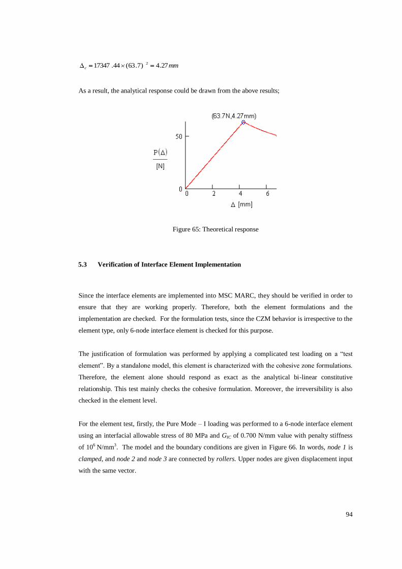
94

mmc 27.4)7.63(44.17347 2

As a result, the analytical response could be drawn from the above results;

Figure 65: Theoretical response

5.3 Verification of Interface Element Implementation

Since the interface elements are implemented into MSC MARC, they should be verified in order to

ensure that they are working properly. Therefore, both the element formulations and the

implementation are checked. For the formulation tests, since the CZM behavior is irrespective to the

element type, only 6-node interface element is checked for this purpose.

The justification of formulation was performed by applying a complicated test loading on a ―test

element‖. By a standalone model, this element is characterized with the cohesive zone formulations.

Therefore, the element alone should respond as exact as the analytical bi-linear constitutive

relationship. This test mainly checks the cohesive formulation. Moreover, the irreversibility is also

checked in the element level.

For the element test, firstly, the Pure Mode – I loading was performed to a 6-node interface element

using an interfacial allowable stress of 80 MPa and GIC of 0.700 N/mm value with penalty stiffness

of 106 N/mm3. The model and the boundary conditions are given in Figure 66. In words, node 1 is

clamped, and node 2 and node 3 are connected by rollers. Upper nodes are given displacement input

with the same vector.

95

Figure 66: The model and the boundary conditions of standalone model for mode I test.

Prior to any run on the test element, the analytically critical displacement is supposed be calculated

by using Eqn. (26) that gives

mmMPa

N/mmIc 0175.0

80

700.02

Hence, the response of the element should reveal both the interfacial stress, and the maximum

displacement within the interpenetration prevention ability. In scope of those items, Figure 67 shows

the input and the response of the element.

96

(a)

(b)

Figure 67: Pure Mode check-run (b) input and (a) output.

It is seen from Figure 67 that from points A and B, the unloading curve successfully works. Also, the

interpenetration ability works well if one considers the point C. Moreover, after reloading the curve

to B and D, the ―consumed‖ energy that spawns irreversibility is also working as expected. The

numerical results, involving stresses and displacements, are almost exact with the analytical

calculation. Hereby, it can be declared that the interface element behaves perfect for pure mode I.

Similarly, the same check is performed for the mixed-mode loading. The mixed-mode ratio β of 2.0

with 80 MPa of opening, 100 MPa of shearing interfacial strength and 0.7 N/mm of GIC, 1.7 N/mm

of GIIC and α = 2.0 for the quadratic failure are the parameters that is used for the mixed-mode

loading test. The model and the boundary conditions are given in Figure 68Figure 66. In words, all

lower nodes are clamped. Upper nodes are given displacement input with the same vector for both

mode I and mode II directions.

97

Figure 68: The model and the boundary conditions of standalone model for mixed-mode test.

The corresponding analytical results can be found by using Eqn. (25);

mmmmN

MPamm

mmN

MPaIIoIo

4

3

4

31010

/100000

100and108

/100000

80

Then using Eqn. (29), one may find the onset of delamination as follows;

mmmmmm

mmmmo

4

2424

244 1048.9

)1080.2()1010(

0.211081010

Eqn. (33) gives the critical displacement;

mmmm

c 038.07.1

0.2

7.0

1

101048.9

)0.21(22/1

222

54

2

The corresponding pure mode failure parameters are finally calculated from Eqns.(28) and (30);

o4.630.2)tan(

Yielding,

mm 017.0)4.63cos(mm 038.0M

Ic

mm 034.0)4.63sin(mm 038.0M

IIc

98

In the highlight of the above results, the response of the test element can be compared on Figure 69.

Both the numerical results and the features like irreversibility, reloading, unloading and the

interpenetration prevention, seem to be working properly if one investigates the results carefully. It

is not necessary to continue for other mixed-mode ratios values because the mixed-mode ratio is

nothing but a constituent of the formulations.

(a)

(b)

Figure 69: Mixed Mode (with β = 2.0) check run input and response

99

As a result, the cohesive formulation works perfect inside the element also in mixed-mode loading.

Noting that, the stresses and displacements are irrelevant to the element type since the loading is

introduced by a displacement input.

In terms of the element behavior, the formulation works successfully, the only remaining check is

the response of the element in the whole FE model. As a result, one may check the element

integration procedures that are formulated, like the element stiffness matrix and the internal force.

To do that, for 40 MPa of interfacial stress, with GIC = 0.352 N/mm and by a penalty stiffness of 106

N/mm3, the DCB model run described in the previous sections was performed. It should be noted

that, although the original interfacial stress was 60 MPa, instead 40 MPa is used because of the

guaranteed converged solutions as mentioned in the following paragraphs.

(a)

(b)

Figure 70: Stress distribution in vicinity of crack tip.

Lcz≈ 1.25 mm

100

The response and the corresponding behavior of the element are summarized in Figure 70. The

―wavy‖ traction profiles on the crack tip area seen Figure 73b, is in accordance with the behavior in

Figure 37. Subsequently, it can be concluded that the behavior is nearly the same with the one given

in Figure 37. The vital point is the crack tip traction behavior at the critical load point. As the

traction becomes zero at the tip point, oscillations start at the global response.

Numerically, the critical load, limiting the uncontrolled delamination growth, was extracted from the

MARC output file. The critical load Pc is 64.8 N and the critical displacement Δc is 4.65 mm. On the

other hand, the theoretical critical load and the displacement are 63.7 N and 4.27 mm, respectively.

The difference is quite small for both results. Note that, the difference in the critical load is more

important than the difference in the critical displacement. This is due to the fact that the

displacement is mainly driven by the beam theory assumption. On the other hand, the load is

determined by the cohesive region.

However, after the critical load, the system does hardening instead of softening. In other words, on

the load-displacement curve, as the displacement increases, the load increases after the critical point.

This erroneous reaction is going to be discussed elaborately in the next chapter.

As a further study, the cohesive zone length can be extracted for the weakened interfacial trial as

1.25 mm (Figure 70). From the Eqn. (15), one may find the appropriate M value as follows;

52.025.1)()40(

/352.011000

2MmmM

MPa

mmNMPalcz

This value is between Dugdale/Barennblat and Rice/Falk values (Table 1). Therefore, our specific

case should use M = 0.52 to define the cohesive zone length in plane strain assumption.

101

CHAPTER 6

6 RESULTS AND DISCUSSION

This study aimed to investigate CZM in terms of the latest advancements so as to reach the best

CZM interface element. The criteria for the investigation are based on accuracy and performance.

The performance of a feature is based on convergence characteristics and solution time of the

processor. On the other hand, the accuracy criterion is based on the comparison with FEA results

and the analytical approximations. In addition, the expected errors with the analytical approximate

results are also referred to the same studies in literature.

The results and discussions of this study can be considered over the following items:

I. Comparative Analysis of Unified Mode Approach vs. Separated Mode Approach

II. Investigation of Artificial Modifications for Improving Convergence

a. Comparative Analysis of Models Using 6-Node Quadratic and 4-Node Linear Interface

Elements

b. Effects of Decreasing Interfacial Strength and Penalty Stiffness

III. Discussion about Convergence Performance

These issues are discussed in the following sections.

6.1 Comparative Analysis of Unified Mode Approach vs. Separated Mode Approach

The approaches of Unified Mode Approach (UMA) [3-4,12,68] and Separated Mode Approach

(SMA) [1,2,21,59] have similar yet with unique characteristics. Therefore, their contrasts are

discussed and investigated in terms of the accuracy and convergence performance.

Specifically, UMA uses direct application of initiation criterion of BK and it takes the total

displacement as a damage parameter, whereas, SMA defines new damage parameter using pure

mode displacements. Also, SMA does not involve BK criterion, instead; quadratic criterion is used.

Actually, SMA uses power criterion due to the fact that the formulations in SMA is based on only

102

the pure mode parameters. Since BK criterion requires mixed-mode parameters, SMA is not suited

for BK criterion. Moreover, another difference is the modification in which SMA approach adjusts

the penalty stiffness values for each pure mode (Eqn. (100)). As mentioned in Appendix B, this

modification is required for SMA in order to sustain the failure instant same for both of the shear

modes and the opening mode. Otherwise, mode I and shear mode cannot be failed at the same

instant; as a result, compatibility is not ensured.

Due to those differences, the tangent stiffness matrix becomes different between SMA and UMA.

The tangent stiffness matrix is quite an important feature for the convergence performance if one

recalls the arc-length method. To show the differences in the tangent stiffness matrix, the best way is

to show the tangent stiffness matrices of both approaches, schematically.

Figure 71 illustrates a typical tangent stiffness matrix for UMA, schematically. The horizontal and

the vertical axis are Node i and the degrees of freedoms, in which Mode I means the opening degree

of freedom and Mode II implies shearing degrees of freedom (DOF). The orange boxes with P sign

indicate that the stiffness in the box has the same sign with the stiffness value calculated by Eqn.

(43). Obviously, N sign indicates the opposite. One may reveal that the orange boxes with P values

form a symmetry line for the tangent stiffness matrix.

Mode I Mode II Mode I Mode II Mode I Mode II Mode I Mode II Mode I Mode II Mode I Mode II

Mode I P 0 0 0 0 0 0 0 0 NMode II P 0 0 0 0 0 0 0 0 NMode I 0 0 P 0 0 0 0 N 0 0

Mode II 0 0 P 0 0 0 0 N 0 0

Mode I 0 0 0 0 P N 0 0 0 0

Mode II 0 0 0 0 P N 0 0 0 0

Mode I 0 0 0 0 N P 0 0 0 0

Mode II 0 0 0 0 N P 0 0 0 0

Mode I 0 0 N 0 0 0 0 P 0 0

Mode II 0 0 N 0 0 0 0 P 0 0

Mode I N 0 0 0 0 0 0 0 0 PMode II N 0 0 0 0 0 0 0 0 P

: Non-Symmetric Terms

P : Positive terms

N : Negative Terms (N = -P)

Node 1

Node 2

Node 3

Node 4

Node 5

Node 6

Node 1 Node 2 Node 3 Node 4 Node 5 Node 6

Figure 71: Element Tangent Stiffness Matrix representation of UMA (for 6-node interface elm.)

As the mixed-mode ratio (Eqn. (11)) increases after initiation of the delamination, local non-

symmetric terms, shown as pink boxes in Figure 71, emerge and increase, accordingly. The word

―local‖ is used for naming the terms because these non-symmetric terms do not influence the overall

symmetry of tangent stiffness matrix. On the other part, the word ―non-symmetric― is used because

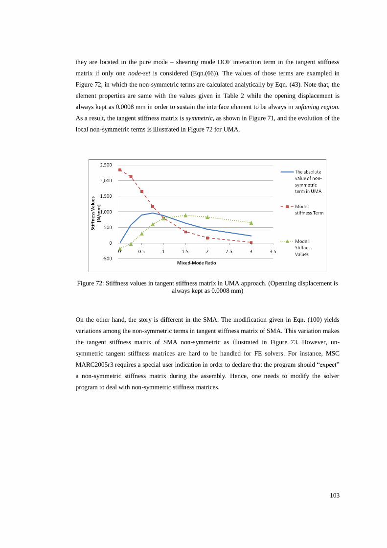
103

they are located in the pure mode – shearing mode DOF interaction term in the tangent stiffness

matrix if only one node-set is considered (Eqn.(66)). The values of those terms are exampled in

Figure 72, in which the non-symmetric terms are calculated analytically by Eqn. (43). Note that, the

element properties are same with the values given in Table 2 while the opening displacement is

always kept as 0.0008 mm in order to sustain the interface element to be always in softening region.

As a result, the tangent stiffness matrix is symmetric, as shown in Figure 71, and the evolution of the

local non-symmetric terms is illustrated in Figure 72 for UMA.

Figure 72: Stiffness values in tangent stiffness matrix in UMA approach. (Openning displacement is

always kept as 0.0008 mm)

On the other hand, the story is different in the SMA. The modification given in Eqn. (100) yields

variations among the non-symmetric terms in tangent stiffness matrix of SMA. This variation makes

the tangent stiffness matrix of SMA non-symmetric as illustrated in Figure 73. However, un-

symmetric tangent stiffness matrices are hard to be handled for FE solvers. For instance, MSC

MARC2005r3 requires a special user indication in order to declare that the program should ―expect‖

a non-symmetric stiffness matrix during the assembly. Hence, one needs to modify the solver

program to deal with non-symmetric stiffness matrices.

104

Mode I Mode II Mode I Mode II Mode I Mode II Mode I Mode II Mode I Mode II Mode I Mode II

Mode I P ● 0 0 0 0 0 0 0 0 N ●

Mode II P 0 0 0 0 0 0 0 0 NMode I 0 0 P ● 0 0 0 0 N ● 0 0

Mode II 0 0 P 0 0 0 0 N 0 0

Mode I 0 0 0 0 P ● N ● 0 0 0 0

Mode II 0 0 0 0 P N 0 0 0 0

Mode I 0 0 0 0 N ● P ● 0 0 0 0

Mode II 0 0 0 0 N P 0 0 0 0

Mode I 0 0 N ● 0 0 0 0 P ● 0 0

Mode II 0 0 N 0 0 0 0 P 0 0

Mode I N ● 0 0 0 0 0 0 0 0 P ●

Mode II N 0 0 0 0 0 0 0 0 P

: Non-Symmetric Terms P : Positive terms

● : Varied non-symmetric term N : Negative Terms (N = -P)

Node 1

Node 2

Node 3

Node 4

Node 5

Node 6

Node 1 Node 2 Node 3 Node 4 Node 5 Node 6

Figure 73: Element Tangent Stiffness Matrix representation of SMA (for 6-node interface elm.)

Furthermore, the variation between a ―dotted‖ pink box and a ―clean‖ pink box is not negligible. For

the same conditions used for Figure 72, the evolution of difference between adjacent ―dotted‖ and a

―clean‖ pink boxes are given in Figure 74. If one compares the numerical values of Figure 72 and

Figure 74, it can be revealed that the difference in non-symmetric tangent stiffness matrix is not

negligible. Therefore, this may yield a handicap for SMA in terms of convergence performance.

Figure 74: Absolute difference between a ―dotted‖ pink box and a ―clean‖ pink box for SMA.

For the accuracy point of view, The Tip Force – Displacement curves of the both approaches and the

approximate analytical solution is given in Figure 75. For the accuracy point of view, both

approaches result in nearly identical Tip force – displacement curve for the DCB test of our study

(Table 2).

105

Figure 75: Tip force versus displacement response of UMA and SMA.

As a summary, it seems like the tangent stiffness matrices are different for the both of the

approaches. Hence, the convergence performance and the overall performances might be different

for mixed-mode cases.

6.2 Investigation of Artificial Modifications for Improving Convergence

In literature, researchers study for improving the convergence performance of the interface elements.

In addition to the convergence, elapsed time for the solution of a run should also be considered. To

cope with them, there are modifications for interface element material definitions and various types

of interface elements [87-88,95]. As a broad discussion for them, the results of the below items are

going to be discussed in this section.

6.2.1 Comparative Analysis of Models Using 6-Node Quadratic and 4-Node Linear

Interface Elements

There are two runs involving identical arc-length and material parameters, yet with disparities only

in the resulting meshes. The difference is morphological in the resulting meshes and emerged due to

the elements used for modeling the body of the DCB. In 6-node interface elements, 8-node body

elements are used as given in Chapter 5.2.2.1. On the other hand, 4-node interface element requires

4-node elements as presented in Appendix A. As a result, number of nodes used in the model is

different. Moreover, the elements used in the interfaces are different in terms of the order of the

shape function. Consequently, the comparison is performed; depending on convergence

106

performance, solution duration and response of the tip force – displacement curve (accuracy). It

should be noted that the penalty stiffness is taken as 104 N/mm3 instead of 106 N/mm3 for all of the

runs in order to guarantee the convergence.

The results of the runs reveal that the model using 6-node interface elements requires less time to

finish the job as shown in Table 4. On the contrary, Table 4 stresses that the model using 4-node

interface elements requires less number of increments to solve the model. Hence, even though the 6-

node model requires more increments to finish the run, the time elapsed to finish the job is lower.

Table 4: Time and Increments to finish a job

(Performed in Intel Pentium Core2 6400 @ 2 x 2.13 GHz, 3 GB Ram)

Time Elapsed Inc. to Finish

4-node 28:58 347

6-node 18:14 411

Another performance criterion is the number of cycles required for achieving a converge at each

increment. Figure 76 displays the graph of increment versus cycles, which is number of iterations to

reach a converged point in an increment. Figure 76 reveals that 6-node element has more cycles in

total, whereas, 4-node has localized cycles. After a while, the cycles in 4-node model abrubtly drops.

On the other hand, the number of cycles after the critical point is gradually decreasing the model of

6-node interface elements.

Figure 76: Increment vs. required cycles for converganc of increment for element types

107

Actually, the difference in Figure 76 can be expected when Figure 77 is examined thoroughly. It can

be seen that the responses are nearly identical up to Pc. However, after that point, 4-node interface

element model shows tougher and smoother characteristics. Whereas, 6-node one behaves in a

typical oscillating response. However, since the response after the critical load are not correct - due

to the unrealistic hardening -, a discussion about that region may not be correct.

Figure 77: Tip force vs. Displacement response for 4 node linear and 6 node quadratic interface

elements

6.2.2 Effects of Decreasing Interfacial Strength and Penalty Stiffness

The most struggling issue of the CZM method is the possibility to face with low convergence rates.

As suggested in [95] and [43], the number of elements that stay inside the cohesive zone should be

high in order to get improvement in the convergence. On the contrary, as the number of elements is

increased, the solution time for finishing the run is peaked. To cope with this conflict, some

researchers [43,59,95,97] suggest to artificially reduce the interfacial strength to increase the

cohesive zone (Eqn. (15)).

Therefore, by varying the interfacial strength as 10 MPa, 40 MPa and 60 MPa, trials with penalty

stiffness of 106 N/mm3 are performed in order to see the impacts on the results. As pointed out by

the Hallet et al. [43] that, unless the interfacial strength was decreased excessively, the resulting

response would be similar. Actually, this is exactly the same case that we currently have (Figure 78).

108

Figure 78: Tip Force - Displacement response of various interfacial strengths

From Figure 78, it is seen that the trial with 60 MPa interfacial strength does not converge after Pc.

On the other hand, 40 MPa case is converged after Pc. Finally, the interfacial strength of 10 MPa

gives no convergence problem and without any high cyclic oscillations that shows better solution

times. However, the result would be extremely soft, and hence; the solution was stopped manually.

The similar effect is observed, when the different penalty stiffness values is varied. As discussed

before, penalty stiffness has a significant effect on convergence and the response of the structure as

shown in Figure 47. Our study summarized trial runs in Figure 79 for 60 MPa interfacial strength on

6-node interface element model.

109

Figure 79: Sensitivity results of penalty stiffness values.

From Figure 79, although lower the penalty stiffness values greatly benefits the convergence rates,

they would overshoot as in the 5x103 or yield ―no softening‖ response like in 103. Perhaps, it would

be better to keep the penalty stiffness above 104 N/mm3 which is also a suggestion for some authors

other than Turon et al. [96]. Moreover, the results are quite similar with the results shown in Figure

47.

6.3 Discussion on Convergence Performance

During the study, convergence was one of the major problems encountered, especially after the

critical loading attained. This can be identified easily in Figure 80 which shows time versus cycles

and cutbacks required to get converged results for the model using 6-node interface elements.

Cutbacks happen in the cases where the number of iterations exceeds the limit that the user defines

as a divergence criterion. In other words, a cutback is the phase where the radius of the arc-length is

modified (Eqn. (86)). Therefore, the number of cutbacks in an increment can be a measure for

criticizing the performance of a run. As seen from the Figure 80b, the number of cutbacks peaked

after the critical load is achieved. Noting that, the cutbacks are given in cumulative way, such that, as

the new cutbacks are formed, they are added to the previous cutbacks. From this point of view, it is

expected to see linearly increasing cutbacks after the critical load. Therefore, the behaviors in the

Figure 80a and Figure 80b can be expected.

110

(a)

(b)

Figure 80: Cycle and Cutback segregation throughout the solution.

The number of cycles is also a measure for considering the convergence performance. It can be seen

from Figure 80a that after the critical load achieved, the number of cycles to reach converged points

is peaked and remained same.

Therefore, from the cutback vs. time parameter graph (Figure 80b) and the cycle vs. time parameter

graph (Figure 80a), it can be summarized that after critical load achieved, the convergence

111

performance is lowered and retained with the ―lowered value‖ throughout the remaining analysis.

Hence, it could be said that there are two regions in terms of convergence during the solution;

―before the critical load‖ and ―after the critical load‖. Also, these two regions have negligible

variations inside.

112

CHAPTER 7

CONCLUSIONS

Cohesive Zone Method (CZM) is widely investigated, and the study is mainly focused on finite

element application of the method. In fact, the motivation is to achieve a CZM interface element;

having high accuracy, high convergence characteristics, and consequently; high overall performance.

Our study is aimed to be a preliminary study for this objective.

The investigation about CZM is started with a discussion about the theory in comparative way

among the other methods of delamination propagation. Especially, a broad theoretically comparative

discussion between Virtual Crack Closure Technique (VCCT) and CZM is given. It is concluded that

CZM is more efficient and more capable than VCCT. Besides, the selected numerical solution

scheme; the arc-length method is also re-derived from well known Newton-Raphson method. In

parallel, the convergence issue and the importance of the numerical solution scheme is discussed.

The two main approaches for CZM formulations are categorized as; Unified Mode Method (UMA)

and Separated Mode Approach (SMA). Accordingly, they are compared and contrasted numerically

in a finite element model of DCB test. On the other hand, the differences in tangent stiffness

matrices of the two approaches are brought out, theoretically. The formation of non-symmetric

tangent stiffness matrices for SMA is revealed in high mixed-mode ratios. Next, the artificial

modifications improving convergence performance; using 6-node quadratic interface elements

instead of 4-node linear interface elements, reducing the penalty stiffness and the interfacial strength

are investigated.

It is observed that the approaches of UMA and SMA result in identical accuracy for the DCB test

model [70]. However, the key point for the convergence performance is the element tangent stiffness

matrix. At this point, it is theoretically shown that SMA is prone to form non-symmetric tangent

stiffness matrices in high mixed-mode ratios, β. Moreover, it is also shown that the non-symmetric

tangent stiffness matrix of SMA is in considerable values and hence; it is suggested taking this effect

into account by applying mixed-mode loading cases. It is highlighted that handling of non-

symmetric stiffness matrices can make SMA a cumbersome approach. For the tip force-

displacement curve of the DCB model, after the critical point is reached, the different oscillatory

113

behaviors are observed for each approach. However, since the response on that region is not correct

due to the hardening behavior, such a discussion about oscillatory response is not applicable.

The models, using interface elements of 4-node linear or 6-node quadratic elements, were compared

in terms of convergence rates, overall performance and accuracy. The results show that the model

using 4-node interface element requires fewer increments, yet with longer solution duration to finish

a job. This contradictory result could be occurred because of two differences between two models;

the first is the number of interface elements and secondly, the morphological differences.

Low number of increments to finish a job can be assumed to mean a better convergence rate.

Therefore, the model using 4-node interface elements can be considered the one having the best

convergence rate. This result is happened possibly due to the fact that, the total number of 4-node

interface elements is twice the number of 6-node interface elements used in their corresponding

models. In other words, there are two times more interface elements used in the model with 4-node

interface elements. Recalling from the Section 5.2.2.1 and Appendix A, the models of 4-node and 6-

node interface elements are somehow ―correlated‖ by having the same aspect ratios of the elements.

Consequently, using twice number of interface elements might have improved the convergence rate

of the model using 4-node interface element, even though the order of the 4-node linear interface

element is lower than the 6-node quadratic interface element.

On the other part, the model using 6-node interface elements requires less time to finish the job. The

reason might be due to the requirement of an additional node to ―convert‖ one 8-node body element

into four 4-node body elements. This phenomenon is best illustrated in Figure 81. The additional

node – displayed as shaded in the middle of the Figure 81– is required to put four 4-node quad body

elements to fill the volume of one 8-node body element. Actually, this is the reason of the

morphological difference between the two models. Consequently, the model using 4-node interface

elements has more nodes, and hence; yields more degrees of freedom in the assembled stiffness

matrix. In our case, there is 27.2% (exactly 5232) more degrees of freedom in the assembled

stiffness matrix of the model using 4-node linear interface elements. Consequently, more degrees of

freedom might result in the higher computational duration.

114

Figure 81: 8-node element ―hatches‖ four 4-node elements with one additional node emerged at the middle.

Next, the weakening of interfacial strength and lowering the penalty stiffness are examined so as to

find appropriate modifications leading to an effective interface element. By direct investigation of

the results, one may declare that they give quite parallel results regarding to the similar studies

performed in literature [12,43,59,72,96].

A decrease in interfacial strength gives better convergence rates and yet, still accurate results if the

decrease is ―under control‖. Otherwise, after a certain value, it is observed that the model starts to

give inaccurate results. For the instance of the DCB test performed by Morais et al. [70], it is

obtained that an interfacial strength of 10 MPa results in excessively soft response (Figure 78). It

seems like 40 MPa gives good results since the critical load is identical to the one obtained for the

actual 60 MPa case (Figure 78). It should be noted that the weakening of the interfacial strength may

give over-estimated allowable for delamination onset [39]. However, since our study does not

analyze initiation of delamination cracks, possible influences of weakening the interfacial strength

on the delamination initiation are automatically skipped.

Likely observed for the weakening of the interfacial strength, decrease in the penalty stiffness has a

similar effect. In fact, this is the reason why they are considered in the same section in our study. For

the penalty stiffness of 5x103 N/mm3, the result spawns overshot critical load whereas, the others

above 104 N/mm3 highlights identical critical loads as seen for all of the models (the DCB test

performed by Morais et al. [70]). An excessively soft penalty stiffness of 103 N/mm3 behaves like the

interfacial strength of 10 MPa with inaccurate and excessively softened results in our model.

Perhaps, it would be convenient to use a penalty stiffness of 104 N/mm3 or 40 MPa of interfacial

strength to get rid of the fine mesh requirement in this test. Namely, it is suggested that by using

lower penalty stiffness and weaker interfaces, it would not need to model with cumbersome fine

meshes. In fact, this conclusion is agreed by the literature [12,43,59,72,96].

During the study, one of the most challenging points experienced is divergence. It is experienced that

MARC 2005r3 has awful characteristics in terms of convergence ability. First of all, MARC does not

115

have the Modified Arc-Length Method which is specialized in dealing with sharp snap backs

[18,61]. This modified method has a better root selection scheme that also considers residuals to

catch snap backs instead of only checking the minimum angle [18]. Therefore, the Arc-Length

Method inside MARC 2005r3 is old-fashioned. Moreover, MSC MARC 2005r3 does not have a

procedure like, viscous regularization [24,27], which improves convergence by ―damping‖ the

tangent stiffness matrices of softening constitutive relationships. Therefore, although the suggestions

of Turon et al. [96] were followed during our study, the convergence still became a problem.

As a result of numerical results of the finite element analysis and the verifications, it can be

concluded that, there is no problem in embedding the CZM formulation. Hence, the results are

satisfactory and adequate to declare that the formulations have been successfully implanted into

MSC MARC 2005r3. Also, all of the foregoing runs show the same and the correct critical force and

critical displacement values. However, only the overall response of the structure after the critical

load, Pc, is not correct. In our study, after the critical load reached, there is no softening of the

structure, which is supposed to cause ―uncontrolled‖ crack propagation. Since the critical load is

checked in terms of detailed cohesive zone analysis by the interface element traction-displacement

evolution curves, the results are reasonable. The error could be emerged from an error accumulation

during the numerical solution scheme. Therefore, a further investigation with lower residual

tolerances is required in the region after critical loading. Actually, this is the only deficiency of our

study that requires further investigation.

Additionally, widely used commercial program, like ABAQUS [24], could be used in order to see

whether the error is occurred because of the MSC MARC 2005r3. This is reasonable because the

―communication‖ between the user-subroutine and the solver, or any other programming error might

be the problem. Moreover, the usage of user-subroutines in literature is more common for ABAQUS.

In brief, the mitigation could be to change the commercial FEA program and check possible

programming problems.

For the last but not the least, this study needs to be developed further to enhance the convergence

issue, and understanding the over-stiff response after critical load it needs the application of more

tests like ENF, MMB to acquire more knowledge to further clarify the above issues. Moreover,

implementing the interface elements into other commercial programs, possible problems emerged by

MSC MARC2005r3 would diminish. In either way, the findings in this study promise many aspects

of fields to investigate more in deeply.

116

CHAPTER 8

FUTURE WORKS

The study definitely requires solving the erroneous response after the critical load is achieved. The

same formulations are going to be implemented into ABAQUS which is widely used by researchers.

If the problem still exists, than by comparing the inherent interface elements already implemented

into ABAQUS, it would yield a chance to understand any error output of the developed interface

element.

It seems like the global effect of utilization of interface elements could be studied more deeply.

Generally, the general view of a method is overlooked by researchers. Therefore, it would be better

to study on the global performance of a model in the scope of selecting the appropriate interface

element. In addition, the differences of the approaches concerned in our study could be investigated

in terms of performance characteristics by set of MMB test models. As a result, the effects of non-

symmetric tangent stiffness matrices for SMA could be revealed.

For a longer term, nowadays Nano-Composite structures are modeled by constitutive relationships in

finite element models. Representative elements are being developed on this field. The experience in

this thesis might be continued to high performance develop representative elements for the field of

nano-materials like nano-composites.

7

117

8

9 REFERENCES

[1] Alfano G, Crisfield MA. Finite Element Interface Models for the Delamination Analysis

of Laminated Composites: Mechanical and Computational Issues. International Journal for

Numerical Methods in Engineering 2001;50:1701-1736.

[2] Alfano G, Crisfield MA. Solution Strategies for the Delamination Analysis Based on a

Combination of Local-Control Arc-Length and Line Searches. International Journal for

Numerical Methods in Engineering 2003;58:999–1048.

[3] Allix O, Corigliano A. Modeling and Simulation of Crack Propagation in Mixed-Mode

Interlaminar Fracture Specimens. International Journal of Fracture 1996;77:111–140.

[4] Allix O, Ladeveze P, Corigliano A. Damage Analysis of Interlaminar Fracture Specimens.

Composite Structures 1995;31:61-74.

[5] Anderson TL. Fracture Mechanics: Fundamentals and Applications, 2nd Ed. CRC Press

LLC 1995.

[6] Ao ki Y, Suemasu H, Ishikawa T. Damage Propagation in CFRP Laminates Subjected to Low Velocity Impact and Static Indentation. Advanced Composite Materials 2007;16:45–

61.

[7] ASTM Standard D5528. Standard Test Method for Mode I Interlaminar Fracture Toughness

of Unidirectional Fiber – Reinforced Polymer Matrix Composites. ASTM International,

West Conshohocken PA; 2007.

[8] Barenblatt GI. Mathematical Theory of Equilibrium Cracks in Brittle Failure. Advances in

Applied Mechanics 1962;7.

[9] Benzeggagh ML, Kenane M. Measurement of Mixed-Mode Delamination Fracture

Toughness of Unidirectional Glass/Epoxy Composites with Mixed-Mode Bending

Apparatus. Composites Science and Technology 1996;56:439–449.

[10] Beuth JL. Separation of Crack Extension Modes in Orthotropic Delamination Models.

International Journal of Fracture 1996;77:305–321.

[11] Bouvard JL, Chaboche JL, Feyel F, Gallerneau F. A Cohesive Zone Model for Fatigue and

Creep–Fatigue Crack Growth in Single Crystal Superalloys. International Journal of Fatigue 2009;31:868–879.

118

[12] Camanho PP, Davila C. Mixed-Mode Decohesion Finite Elements for the Simulation of

Delamination in Composite Materials, NASA/TP-2007-214869 2002.

[13] Camanho PP, Davila CG, Ambur DR. Numerical Simulation of Delamination Growth in Composite Materials, NASA/TP-2001-211041 2001.

[14] Chen J. Predicting Progressive Delamination of Stiffened Fibre-Composite Panel and

Repaired Sandwich Panel by Decohesion Models. Journal of Thermoplastic Composite

Materials 2002;15: 429.

[15] Chen J, Crisfield M, Kinloch AJ, Busso EP, Matthews, Qui Y. Predicting Progressive

Delamination of Composite Material Specimens via Interface Elements. Mechanics of

Composite Materials and Structures 1999;6:301-317.

[16] Chen J, New A. Application of Decohesive Model with Mixed Damage Scale in Fracture

Analysis of Composite Materials. Blackwell Science Ltd. Fatigue Fract Engng Mater Struct

2001;24:761–769.

[17] Chen J. Predicting Progressive Delamination of Stiffened Fibre-Composite Panel and

Repaired Sandwich Panel by Decohesion Models. Journal of Thermoplastic Composite

Materials 2002;15:429.

[18] Crisfield MA. A Fast Incremental Iterative Solution Procedure that Handles Snap Through. Computers & Structures 1982;25:823-829.

[19] Crisfield MA. An Arc-Length Method Including Line Searches and Accelerations.

International Journal of Numerical Methods in Engineering 1983;19:1269-1289.

[20] Crisfield MA, Jelenic G, Mi Y, Zhong H. –G, Fan Z. Some Aspects of the Non-Linear

Finite Element Method. Finite Elements in Analysis and Design 1997;27:19-40.

[21] Crisfield MA, Hellwerg HB, Davies GAO. Failure Analysis of Composite Structures Using

Interface Elements. Proceedings of the NAFEMS Conference on Application of Finite

Elements to Composite Materials (London, U.K.) 1994:1-4.

[22] Crisfield MA. Non-linear Finite Element Analysis of Solids and Structures. John Wiley &

Sons 1994.

[23] Cui W, Wisnom MR. A Combined Stress Based and Fracture Mechanics Based Model for

Predicting Delamination in Composites. Composites 1993;24:476-474.

[24] Dassault Systèmes [Internet], Providence (RI): The company; c2004 – 2009. Abaqus 6.9

New and Enhanced Features Addendum; [cited 2009 Aug 15]. Available from:

http://www.simulia.com/download/pdf/Abaqus69_Addendum_final.pdf

[25] Davidson BD. Prediction of Energy Release Rate for Edge Delamination Using a Crack Tip

Element Approach. Composite Materials: Fatigue and Fracture, ASTM STP 1230, R.H.

Martin, Ed., American Society for Testing and Materials 1995;5:155–175.

119

[26] Davidson BD, Bialaszewski RD, Sainath SS. A Non-Classical, Energy Release Rate Based

Approach for Predicting Delamination Growth in Graphite Reinforced Laminated

Polymeric Composites, Composites Science and Technology 2006;66:1479–1496.

[27] Davila C, Camanho PP, Turon A. Cohesive Elements for Shells. NASA/TP-2007-214869

2007.

[28] De Borst R. Fracture in Quasi-Brittle Materials – A Review of Continuum Damage-Based

Approach. Engineering Fracture Mechanics 2002;69:95–112.

[29] De Borst R. Numerical Aspects of Cohesive-Zone Models. Engineering Fracture Mechanics

2003;70:1743–1757.

[30] De Morais AB, De Moura MF, Marques AT, De Castro PT. Mode-I Interlaminar Fracture

of Carbon/Epoxy Cross-PlyComposites. Composites Science and Technology 2002;62:679–

686.

[31] De Moura MF, Gonçalves PM, Marques AT, De Castro PMS. Prediction of Compressive

Strength of Carbon-Epoxy Laminates Containing Delamination by Using a Mixed-Mode

Damage Model. Composite Structures 2000;50:151-157.

[32] De Xie A, Waas M. Discrete Cohesive Zone Model for Mixed-Mode Fracture Using Finite

Element Analysis. Engineering Fracture Mechanics 2006;73:1783–1796.

[33] De Xie, Sherrill BB Jr. Strain Energy Release Rate Calculation for a Moving Delamination

Front of Abitrary ShapeBased on the Virtual Crack Closure Technique Part I: Formulation

and Validation, Engineering Fracture Mechanics 2006;73:771–785.

[34] De Xie, Sherrill BB Jr. Strain Energy Release Rate Calculation for a Moving Delamination

Front of Abitrary Shape Based on the Virtual Crack Closure Technique Part II: Sensitivity

Study on Modeling Details, Engineering Fracture Mechanics 2006;73:786–801.

[35] Destuynder PH, Nevers TH. Un modèle de calcul des forces dedélaminage dans les plaques

minces multicouches. J. Méca. Théor.Appliquée 1987;6:179–207.

[36] Dugdale DS. Yielding of Steel Sheets Containing Slits. Journal of Mechanics and Physics

of Solids, 1960;8:100-104.

[37] Elices M, Guinea GV, Gomez J, Planas J. The Cohesive Zone Model: Advantages,

Limitations and Challenges. Engineering Fracture Mechanics 2002;69:137–163.

120

[38] Elmarakbi A, Hu N, Fukunaga H. Implementation of New Adaptive Cohesive Elements for

the Simulation of Delaminationin Composite Materials in LS-DYNA, Fifth LS-DYNA

Anwenderforum, ULM, 2006.

[39] Goyal KV, Johnson ER, Davila CG, Jaunky N. An Irreversible Constitutive Law for

Modeling the Delamination Process Using Interface Elements. NASA/CR-2002-211758

2002;25.

[40] Griffth AA. The Phenomena of Rupture and Flow in Solids. Philosophical Transactions of

the Royal Society, London; Series 1932;22:163-198.

[41] Gustafson PA, Waas AM. The Influence of Adhesive Constitutive Parameters in Cohesive

Zone Finite Element Models of Adhesively Bonded Joints. International Journal of Solids

and Structures 2009;46:2201–2215.

[42] Han T-S, Ural A, Chen C-S, Zehndere AT, Ingraffea AR, Billington SL. Delamination

Buckling and Propagation Analysis of Honeycomb Panels Using a Cohesive Element

Approach. International Journal of Fracture 2002;115:101–123.

[43] Harper PW, Hallet SR. Cohesive Zone Length in Numerical Simulations in Composite

Delamination. Engineering Fracture Mechanics 2008;75:4774–4792.

[44] Hashemi S, Kinloch AJ, Williams JG. The Analysis of Interlaminar Fracture in Uniaxial

Fibre-Polymer Composite. Proc. Roy. Soc. Lond. 1990;A427:173-190.

[45] Hassan NM, Batra RC. Modeling Damage in Polymeric Composites. Composites: Part B

2008;39:66–82.

[46] Hellen TK. On the Method of the Virtual Crack Extension. Int. J. Num. Eng. 1975;9:187-

207.

[47] Hellweg HL, Crisfield MA. A New Arc-Length Method for Handling Sharp Snap-Backs.

Computers & Structures 1995;66(5):705-709.

[48] Hilleborg A, Modeer M, Peterson PE. Analysis of Crack Formation and Growth in Concrete

by Means of Fracture Mechanics and Finite Elements. Cement and Concrete Research

1976;6:773-782.

[49] Irwin GR. Fracture Handbuck der Physik. Berlin, Springer 1958;6:551–590.

[50] Jimenez MA, Miravete A. Application of the Finite-Element Method to Predict the Onset of

Delamination Growth. Journalof Composite Materials 2004;38:1309.

121

[51] Kruger R, Konig M. Investigation of Delamination Growth Between Plies of Dissimilar

Orientations. ISD-Report 1996;96/5.

[52] Krueger R, Minguet PJ, O’Brien TK. A Method for Calculating Strain Energy Release Rates in Preliminary Design ofComposite Skin / Stringer Debonding Under Multi-Axial

Loading, NASA/TM-1999-209365, ARL-TR-2012, 1999.

[53] Krueger R, Citkovich MK, O’Brien TK, Minguet PJ. Testing and Analysis of Composite

Skin/Stringer Debonding Under Multiaxial Loading. Journal of Composite Materials

2000;34:1263–1300.

[54] Krueger R, O'Brien TK. A Shell/3D Modeling Technique for the Analysis of Delaminated

Composite Laminates. Composites Part A: Applied Science and Manufacturing

2001;32(1):25-44.

[55] Krueger R. The Virtual Crack Closure Technique: History, Approach and Applications.

NASA Icase Report 2002;10.

[56] Krueger R, Minguet PJ. Skin-Stiffener Debond Prediction Based on Computational Fracture

Analysis. NASA/CR-2005-213915 NIA Report 2005;06.

[57] Kutlu Z, Chang FK. Modeling Compressive Failure of Laminated Composites Containing Multiple Through-the-width Delaminations. Journal of Composite Materials 1992;26:350–

387.

[58] Lee SM. An Edge Crack Torsion Method for Mode III Delamination Fracture Testing.

Journal of Composites Technology & Research, 1993;15(3):193-201.

[59] Mi Y, Crisfield MA, Davies GAO, Hellweg HB. Progressive Delamination Using Interface

Elements. Journal of Composite Materials 1998;32:1246.

[60] Mohammadi S, Owen DRJ, Peric D. A Combined Finite/Discrete Element Algorithm for Delamination Analysis ofComposites. Finite Elements in Analysis and Design

1998;28(4):321-336.

[61] MSC.MARC® 2005r3, Theory and User Information, Volume A

[62] MSC.MARC® 2005r3, Element Library, Volume B.

[63] MSC.MARC® 2005r3, Program Input, Volume C

[64] MSC.Software Corporation [Internet], Santa Ana (CA): The company; c2009. MARC

Nonlinear Analysis for Engineering Applications & Manufacturing Processes; [cited 2009

Aug 10]. Available from: http:// www.mscsoftware.com/assets/Marc_DS.pdf

122

[65] Needleman A. A Continuum Model for Void Nucleation by Inclusion Debonding. Journal

of Applied Mechanics 1987;54:525-531.

[66] Needleman A. An Analysis of Intersonic Crack Growth Under Shear Loading. Journal of

Applied Mechanics 1999;66:847-857.

[67] Orifici AC, Thomson RS, Degenhardt R, Bisagni C, Bayandor J. Development of a Finite-

Element Analysis Methadology for the Propagation of Delaminations in Composite

Structures. Mechanics of Composite Materials 2007;43(1).

[68] Ortiz M, Pandolfi A. Finite-Deformation Irreversible Cohesive Elements for Three-

Dimensional Crack-Propagation Analysis. International Journal for Numerical Methods in Engineering 1999;44:1267–1282.

[69] Parks DM. A Stiffness Derivative Finite Element Technique for Determination Crack Tip

Stress Intensity Factors. International Journal of Fracture 1974;10(4):487-502.

[70] Pereira AB, de Morais AB. Mixed Mode I + II Interlaminar Fracture of Carbon/Epoxy

Laminates. Composites: Part A. doi:10.1016/j.compositesa.2007.10.013.

[71] Pinho ST, Iannucci L, Robinson P. Formulation and Implementation of Decohesion Elements in an Finite Element Code. Composites: Part A 2006;37:778–789.

[72] Qui Y, Crisfield MA, Alfano G. An Interface Element Formulation for the Simulation of

Delamination with Buckling. Engineering Fracture Mechanics 2001;68:1755-1776.

[73] Ragon SA, Gürdal Z, Watson LT. A Comparison of Three Algorithms for Tracing

Nonlinear Equilibrium Paths of Structural Systems. International Journal of Solids and

Structures 2002;39(3):689-698.

[74] Raju IS, Crews JH, Aminpour MA. Convergence of Strain Energy Release Rate

Components for Edge-Delaminated Composite Laminates. Engineering Fracture Mechanics

1988;30(3):383-396.

123

[75] Ramm E. Strategies for Tracing the Nonlinear Response Near Limit Points. Nonlinear

Analysis in Structural Mechanics. Springer 1981:68-89.

[76] Reddy Jr ED, Mello FJ, Guess TR. Modeling the Initiation and Growth of Delaminations in Composite Structures. Journal of Composite Materials. 1997;31:812-831.

[77] Reeder R, Crews Jr R. Mixed-Mode Bending Method for Delamination Testing. Published

in AIAA Journal. 1990;28(7):1270-1276.

[78] Remmers JJC, de Borst R, Needleman A. A Cohesive Segments Method for the Simulation

of Crack Growth. Computational Mechanics 2003;31:69–77.

[79] Riccio A, Zarrelli M, Tessitore N. A Numerical Model for Delamination Growth Simulation in Non-Crimp Fabric Composites. Composites Science and Technology

2007;67:3345–3359.

[80] Rice JR. A Path Independent Integral and the Approximate Analysis of Strain

Concentration by Notches and Cracks. Journal of Applied Mechanics, 1968:379-386.

[81] Riks E. The Application of Newton's Method to the Problem of Elastic Stability. Journal of

Applied Mechanics 1972;39:1960-1966.

[82] Riks E. An Incremental Approach to the Solution of Snapping and Buckling Problems. Int.

J. of Solids and Structures 1979;15:529-551.

[83] Robinson P, Galvanetto U, Galvanetto D, Bellucci G, Violeau D. Numerical Simulation of

Fatigue-Driven Delamination Using Interface Elements. International Journal for Numerical

Methods in Engineering. 2005;63:1824–1848.

[84] Robinson P, Song DQ. A Modified DCB Specimen for Mode I Testing of Multidirectional

Laminates. Journal of Composite Materials 1992;26:15-54.

[85] Roudolff F, Ousset Y. Comparison between Two Approaches for the Simulation of

Delamination Growth in a D.C.B. Specimen. Aerospace Science and Technology

2002;6:123–130.

[86] Rybicki EF, Kanninen MF. A Finite Element Calculation of Stress-intensity Factors by a

Modified Crack Closure Integral. Engineering Fracture Mechanics 1987;9:931–938.

[87] Schellekens J, de Borst R. On the Numerical Integration of Interface Elements. International Journal for Numerical Methods in Engineering 1993;36:43-66.

[88] Schellekens J, de Borst R. On the Numerical Modeling of Edge Delamination in

Composites. Key Engineering Materials 1996;121–122:131–160.

124

[89] Shahwan KW, Waas AM. Non-Self-Similar Decohesion along a Finite Interface of

Unilaterally Constrained Delaminations. Proceedings: Mathematical, Physical and

Engineering Sciences 4 1997;53(1958):515-550.

[90] Silva A, De Freitas MJ. Mixed-Mode Delamination Growth of Laminar Composites by

Using Three-Dimensional Finite Element Modeling. Fatigue Fract Engng Mater Struct

2002;26:543-549.

[91] Sun CT, Qian,W. Calculation of Stress Intensity Factors for Interlaminar Cracks in

Composite Laminates. Comp. Sci.Techn. 1997;57:637-650.

[92] SzyszkowskI W, Husband JB. Curvature Controlled Arc-Length Method. Computational Mechanics 1999;24:245-257.

[93] Thouless MD, Yang QD, Measurement and Analysis of the Fracture Properties of Adhesive

Joints. The Mechanics of Adhesion. (edited by D.A. Dillard, A.V. Pocious and M.

Chaudhury) Elsevier Science, Amsterdam 2001:235–271.

[94] Tijssens MGA, Sluys LJ, van der Giessen E. Numerical Simulation of Quasi-Brittle

Fracture Using Damaging Cohesive Surfaces. Eur J Mech: A/Solids 2000;19:761–779.

[95] Turon A, Pedro P, Camanho PP, Costa J, Davila CG. An Interface Damage Model for the

Simulation of Delamination Under Variable-Mode Ratio in Composite Materials.

NASA/TM-2004-213277, 2004.

[96] Turon A, Davila CG, Camanho PP, Costa J. An Engineering Solution for Mesh Size

Effects in the Simulation of Delamination Using Cohesive Zone Models. Engineering

Fracture Mechanics 2007;74:1665–1682.

[97] Tvergaard V, Hutchinson JW. On the Toughness of Ductile Adhesive Joints. Journal of the Mechanics and Physics of Solids 1996;44:789–800.

[98] Warrior NA, Pickett AK, Lourenco NSF. Mixed-Mode Delamination – Experimental and

Numerical Studies. Strain 2003:39;153–159.

[99] Wei Y, Hutchinson JW. Interface Strength, Work of Adhesion and Plasticity in the Peel

Test. International Journal of Fracture 1997;93:315–333.

[100] Wells GN, de Borst R, Sluys LJ. A Consistent Geometrically Non-Linear Approach for

Delamination. Int. J. Numer. Meth. Engng. 2002;54:1333–1355.

125

[101] Wempner GA. Discrete Approximations Related to Nonlinear Theories of Solids. Int. J.

Solids and Structures 1971;7:1581-1599.

[102] Wisnom MR, Chang F-K. Modelling of Splitting and Delamination in Notched Cross-Ply Laminates. Composites Science and Technology 2000;60:2849–2856.

[103] Xu XP, Needleman A. Numerical Simulations of Fast Crack Growth in Brittle Solids.

Journal of Mechanics and Physics of Solids 1994;32(9):1397-1434.

[104] Yang QD., Thouless MD. Mixed Mode Fracture of Plastically-Deforming Adhesive Joints.

International Journal of Fracture 2001;110:175–187.

[105] Yang Q, Cox B. Cohesive Models for Damage Evolution in Laminated Composites. Rockwell Scientific Co., LLC, 1049 Camino Dos Rios, Thousand Oaks, CA 91360, USA,

2005.

[106] Ye L. Role of Matrix Resin in Delamination Onset and Growth in Composite Laminates.

Composites Science and Technology 1988;33:257-277.

[107] Zienkewich OC, Taylor RL. The Finite Element Method, Volume 1: The Basis 5th Ed.

Butterworth-Heinemann, 2000.

126

APPENDIX A

FOUR NODE LINEAR INTERFACE ELEMENT FORMULATION AND MODEL

A.1 The Element Formulation

Although MARC has an inherent 4-node plain strain linear interface element definition (Element 186

[62]), it would be better to construct our own 4-node plain strain element similarly done for 6-node

element in the Chapter 5.1.

The 4-node plain strain linear interface element has 2 integration points as shown in the Figure 82.

The element acts as linear line element which possesses interpolation equation of generalized linear

formulation, can be given as [107];

10)( aa

(90)

(a) (b)

Figure 82: (a) 4-node linear plain strain interface element details (b) Node-set definitions

The shape functions should have same degree given in Eqn. (91). By obtaining zero in the node set

s2, the candidate shape function for node set s1 is;

127

)1()(1 CN

(91)

In order to give unity at node set s1 (ξ = -1), the constant C can be found as;

2

11)11()1(1 CCN

(92)

Similarly, the second shape function could be done accordingly. Hence, the shape function for node

1 and 2 could be summarized as;

)1(2

1)(,)1(

2

1)( 21 NN

(93)

For the element kinematics, a similar rotational formulation could be defined by the same AB line

defined for 6-node quadratic interface element;

2,

2

1414 YYXXA ,

2,

2

2323 YYXXB

(94)

where the Xi and Yi shows the coordinates of the nodes. The angle of misalignment can be defined as

follows;

o

XXXX

YYYY900,tan

4132

41321

(95)

The global relative displacement to global nodal displacement matrix B is similar to the one derived

in 6-node, except the dimensions of the matrix is 2x8 with N1 and N2 defined in Eqn. (93).

For the element integration, the determinant of Jacobian matrix is parallel with the 6-node one as

follows;

128

42/)(

2

4132

2

4132 YYYYXXXXlJDet

(96)

Following it the numerical integration scheme would be Newton-Cotes with 2 integration points

with, H1 = H2 = 1 while and ξ1 = -1, ξ2 = 1 referring to Eqn. (85).

A.2 Model Using 4-Node Linear Interface Elements

The average mesh size is 0.125 mm where the DCB elements are modeled by four node quadrilateral

elements. There are 11224 elements of which 760 interface elements exist. Body elements are

Element 11, which is called arbitrary quadrilateral plane strain element [62] using 2x2 Gaussian

Integration [107]. The number of nodes in the model is 12222 that cover the two degrees of freedom

u and v as shown in Figure 83. Hence, roughly the degrees of freedom are 12222 x 2 = 24444.

Figure 83: Element 11, Arbitrary Quadrilateral Plane Strain Element (―+‖: Integration points, ―□‖:

Nodes) [62].

In order to reduce the number of elements in the mesh, ―bias‖ way of modeling is used as shown in

the below as done for the 6-node case. Similarly, the bias feature is accorded with the aspect ratio

without exceeded above 5 as suggested [61].

129

APPENDIX B

CONSTITUTIVE RELATIONSHIP OF SEPARATED MODE APPROACH

Also, one of the objectives of our study is to compare and contrast the differences between the

studies of Separated Mode Approach and Unified Mode Approach. Also, Separated Mode Approach

(SMA) [1,16,59,72] has unique advancements. Therefore, such differences are mentioned in this

section.

The initial difference is the definition of the damage evolution by proposing a new damage

parameter γ as follows [1];

1

/1

2

IIoIo

I

(97)

Analogy with Eqn. (35), the damage evolution can be controlled by [1]

)(max)(max

tt

(98)

The approach of SMA does not use the delamination onset criterion like elliptical law. As a result,

the most unique characteristic of this approach is that there is no such a parameter of total

displacement, δ. In other words, whole delamination analysis is performed in displacements in pure

modes and it indirectly uses the mixed-mode criterion via those pure mode displacements. Hence,

Chen and New [16] proposed a non dimensional damage parameter λ to define the state of the

damage by using only pure mode displacements and critical displacements, which is defined as;

2

2

2

IIcIc

I

(99)

in which λ becomes unity when the full delamination occurs, whereas, it becomes zero for no

damage.

130

Actually, the definition of damage in terms of pure modes causes delamination failure at different

instants for each pure mode failure. This issue was illustrated by Pinho et al. [71] in Figure 84. On

may realize from the figure that the original constitutive law (―Before Compatibility‖) is not

―consistent‖ in terms of the instant when the full damage attained.

Figure 84: Compatibility of Mode I and Mode II [71].

In order to deal with this problem, Alfano and Crisfield [59] proposed to redefine the delamination

onset displacement in Mode II for the compatibility requirement as follows;

IIc

Ic

IoIIo

IIo

IIc

Io

Ic

(100)

In fact, this definition is indirectly adjusting the penalty stiffness in Mode II which does not yield a

problem since the redefinition is in the orders below 10 [59]. The penalty stiffness in mode II for a

stable interfacial strength in mode II can be found from Eqn. (25) and Eqn. (100) as;

131

IoIIc

IcIcII tE0

(101)

Therefore, the above adjustment of Mode II penalty stiffness would result in a compatible constitute

relationship for SMA as shown in Figure 84 by ―Current SMA‖.

132

APPENDIX C

USER CONTROL IN ARC-LENGTH AND NUMERICAL SOLUTION IN MARC

MSC MARC grants some variables to the users in order to control the arc-length method. Since the

convergence is an important issue, this section is dedicated for giving the details of the arc-length

parameters that are adjusted to reach converged solutions.

In subsequent steps the arc-length can be reduced or increased at the start of a new load step

depending on the number of iterations in the previous step, I0. This number of iterations in compared

with the desired number of iterations, Id which is typically set to 3 or 5 [61]. The new arc-length is

then given by [61]

2 2

0 0

0

( ) ( )new predI

l lI

(102)

Hence, the way of convergence is considered by evaluating the previous increments’ iteration to

consider the new candidate arc length. On the other hand, the convergence could not be attained for

the cases where the maximum number of iterations defined by the user in the AUTO INCREMENT

card of the MARC being exceeded.

In addition to Eqn. (102), MARC has two other controls [61] given by

MINl

lMAX

n

i

1

0 (103)

Therefore, the MAX and MIN values could be set in order to limit the maximum enlargement or the

minimum reduction in the arc-length. In addition to this, maximum load multiplier can also be set

[61].

133

And finally, the residual correction shape is controlled via the absolute or relative type of check.

Since absolute value of the residual is not always the same, best way to control the convergence is by

setting the relative residual force margin with respect to the reaction force [61] as

ToleranceF

g

reaction

n

i

(104)

The above equation can also be written according for moments, yet, moments need not to be checked

in our study. Therefore, the ―Tolerance‖ value is only the tolerance for the forces.

134

CURRICULUM VITAE

PERNOSAL INFORMATION

Surname, Name: Gözlüklü, Burak

Nationality: Turkish (TC)

Date and Place of Birth: 14 August 1983, Ankara

Marital Status: Single

Phone: +90 0532 250 00 96

Email: [email protected]

EDUCATION

Degree Institution Year of Graduation C.GPa

MS METU Mechanical Engineering 2009 3.50

BS METU Mechanical Engineering 2006 3.18

Minor METU Metallurgical and Materials 2006 2.50

Engineering

WORK EXPERIENCE

Year Place Enrollment Project, Position

2007-Present TUSAŞ-Turkish

Aerospace Industries

Inc. (TAI)

Stress Analysis

Engineer

Airbus A350 XWB ―Ailerons‖, Outer

Aileron Stress Analysis Responsible

Airbus A350 XWB ―Ailerons‖, Fatigue

Analysis Responsible

EU 6th Framework Programme: ALCAS,

Stress Analysis Responsible

2006-2007 Aero-Limak Inc. Product Engineer ALGA – Automated Advanced Fuselage

Analysis Program, Program Developer

2005-2006 METU (Volunteer) Formula-G Solar Powered Car Race,

Project, Stress Analysis Responsible.

FOREIGN LANGUAGES

Advanced English (TOEFL 2009 iBT Score: 100/120)

SOCIAL

Martial Arts (having EBMAS-Martial Arts Schools, Wing Tsun Kung-Fu Instructor Certificate)

Boxing

Escrima (Filipino Martial Arts)

Brazilian Jiu-Jitsu (Brazilian Martial Arts)

Scuba Diving (having CMAS One Star Scuba Diver License)

Interest in Quantum Physics, Astro-Physics and Philosophy

Documents

DELAMINATION ANALYSIS BY USING COHESIVE … delamination in laminated composites. In this study, ... Behavior used for cohesion analysis for quasi-brittle fracture