Degrees Are Forever: Marriage, Educational Investment, and

Lifecycle Labor Decisions of Men and Women∗

Mary Ann Bronson†

January 2014.

Abstract

Women attend college today at much higher rates than men. They also select dispro-portionately into low-paying majors, with almost no gender convergence along this marginsince the mid-1980s. In this paper, I explain the dynamics of the gender differences in collegeattendance and choice of major from 1960 to 2010. I document first that changes in returnsto skill over time and gender differences in wage premiums across majors cannot explain theobserved gender gaps in educational choices. I then provide reduced-form evidence that twofactors help explain the observed gender gaps: first, college degrees provide insurance againstvery low income for women, especially in case of divorce; second, majors differ substantiallyin the degree of “work-family flexibility” they offer, such as the size of wage penalties fortemporary reductions in labor supply. Based on the reduced-form evidence, I construct andestimate a dynamic structural model of marriage, educational choices, and lifetime laborsupply. I use the model to analyze the contribution of changes in wages and changes inthe marriage market to the observed educational investment patterns over time. I estimatethat the insurance value of the college degree for women in case of divorce is equivalent toabout 31% of the college wage premium. I also estimate that the share of women choosinghigh-return science and business majors would increase from 34% to 45% if wage penaltiesfor labor supply reductions were equalized across occupations. Finally, I test the effects oftwo sets of policies on individuals’ choice of major: a differential tuition policy that chargesless for science and technical majors, as has been proposed in some states; and interventionsintended to improve work-family flexibility. My results show that some family-friendly poli-cies increase the share of women in science and business majors substantially, while othersfurther widen both college gender gaps.

∗I would like to give special thanks to Maurizio Mazzocco and Dora Costa. Thanks also to Leah Boustan,Moshe Buchinsky, Maria Casanova, Kathleen McGarry, Adriana Lleras-Muney, Sarah Nabelsi, Sarah Reber, andTill von Wachter. Research reported in this paper was supported by the National Institutes of Health underAward Numbers 2T32HD7545-11 and 5T32HD7545-10. The content is solely the responsibility of the author anddoes not necessarily represent the official views of the National Institutes of Health.†UCLA, Department of Economics, Bunche Hall, Los Angeles, CA. Email: mary.ann.bronson@gmail.com.

1

Why do women today invest in a college education at much higher rates than men, whereas

fifty years ago men graduated more frequently? And given their high college attendance rates

today, why do women continue to select disproportionately into lower-paying majors? The main

objective of this paper is to answer these two questions.

Historically, men made up the majority of college students, and earned more than 90% of

all high-paying degrees in science and business. In the 1970s and early 1980s, men and women

converged substantially both in college graduation rates as well as in their choices of college

major, with more women choosing science and business degrees. It has been well-documented

that women reversed the “gender gap” in graduation rates by the mid-1980s and now constitute

the majority of college students, although the reason why this occurred is still an open question.1

What has been less well-documented is that convergence between men and women in choice of

major mostly ceased after the mid-1980s. In 1985, nearly 80% of education degrees and about

85% of degrees in health support fields, but less than 30% of hard science and engineering degrees

were awarded to women. The same is true today.2

The question of why women graduate at much higher rates than men, but with very differ-

ent majors, has implications for a range of individual outcomes, as well as for macroeconomic

outcomes like supply of skill to the labor market. As women outpace men in college attendance,

their low participation in majors like science and engineering contributes to potentially low

supply of science-related skills in the U.S. More generally, the observed patterns, like women’s

higher graduation rates despite lower lifetime labor supply, run counter to the predictions of

a standard human capital investment model (Becker (1962), Ben-Porath (1967), Mincer and

Polachek (1974)), and raise questions about the determinants of returns to different educational

choices for men and women.

In this paper, I explain the dynamics of men’s and women’s educational investments from

1960 to 2010. The paper makes three main contributions. The first contribution is to document

reduced-form evidence about the factors that potentially explain the above-mentioned gender

gaps over time. I do this in three steps. In the first step, I show that changes in the wage

premium over time and differences in major-specific premiums across men and women cannot

readily account for the observed gender differences in college attendance or decisions about

majors.

In the second step, I provide evidence that changes in the marriage market starting in the

1970s changed the relative returns to a college education for men and women. I use quasi-

experimental variation in the timing of unilateral, no-fault divorce law reforms across states

1See, for example, Goldin, Katz, and Kuziemko (2006), Chiappori, Iyigun, and Weiss (2009), Charles andLuoh (2003), Vincent-Lancrin (2006). Today women make up 58% of U.S. college students.

2National Center for Education Statistics, Digest of Education Statistics (2012), Tables 343-365.

2

to document that the reforms increased women’s college graduation rates relative to men, and

made them more likely to select high-paying majors in business and science-related fields. There

is a simple intuition for this finding. Women with high school education or less draw from a

substantially lower wage distribution than men, and are also more likely to have custody of

and financial responsibility for children. A college degree allows women access to higher paid

jobs, providing insurance against very low income realizations for women outside a two-earner

household.

In the final step, I present evidence that majors are characterized not only by different wage

premiums, but also by different levels of “work-family flexibility.” By flexibility I mean that

some majors are associated with occupations that provide easier access to part-time or part-

year work and have lower wage penalties in case of a temporary absence from the workforce

or a reduction of weekly hours worked. I show that college women reduce their labor supply

substantially during their childbearing years, and that these patterns differ across majors and

occupations. The data patterns I document indicate that women are more likely than men both

to take advantage of flexibility associated with some majors, as well as to choose more flexible

majors.

The documented empirical patterns indicate that insurance and flexibility are important

drivers of the gender gaps, but it is difficult to quantify the impact of these factors on the

gender gaps using the reduced-form analysis alone. The main reason for this is that other

variables, like returns to skill, also changed over this time period, and will also affect decisions

about education, labor supply, marriage, and divorce.

To address this, as a second main contribution, I develop and estimate a dynamic structural

lifetime model of individual decisions about education, marriage, and labor supply. The model

is constructed based on the documented data patterns. It follows individuals starting at age 18

over three phases of life: education, work, and retirement.

In the first phase, individuals decide whether or not to go to college. If they go to college,

they choose between two majors. The first major is associated with occupations that have a

high return, but also a high rate of skill depreciation, meaning that individuals incur large wage

penalties for any reductions in labor supply. The second major is associated with occupations

that have a lower return, but also a lower rate of skill depreciation. These differences between

the majors match those observed in the data. Individuals make decisions based on their expected

lifetime utility from each educational choice and their unobserved effort cost of completing each

major.

In the second, working phase of life individuals make decisions about time allocated to market

and home production, marriage and divorce, and savings. If an individual is single, each period

he or she is matched with a potential partner and decides whether to marry. If married, the

3

partners make household decisions jointly, but there is no commitment, meaning that if in some

period the partners are not both better off in the marriage than they would be if they were

single, they divorce (Marcet and Marimon (1992)). There are shocks to marital match quality,

as well as to wages and to fertility. After a fertility shock, the presence of a young child in the

household increases the productivity of hours dedicated to child care and home production. The

final, retirement stage of life, is a simplified version of the working life stage, in which individuals

make decisions only about consumption, home production, and savings. For different cohorts,

decisions over the lifetime and therefore expected returns to education are affected by changes

in the wage structure and by changes in the marriage market after the reform in divorce laws.

The model is estimated using the Simulated Method of Moments. The estimated model

matches well the marriage and labor supply patterns of men and women over the lifecycle, and

educational choices of cohorts over time. It generates a reversal in the gender gap in graduation

rates, and the persistence in the gender gap in majors. In the model, the current differences

in educational choices are generated through the interaction between the gender wage gap and

marriage over the lifeycle. On the one hand, the “insurance” value of the degree drives up the

return to college for women in case of divorce, regardless of the major they choose. As a result,

they graduate at higher rates. On the other hand, conditional on being married, women are more

likely to be the lower wage-earners and therefore more likely to specialize in home production

and child care, since for the household this is the optimal division of labor.3 Because of this,

women are more likely than men to incur wage penalties for reductions in labor supply. As a

result, they select majors that offer more flexibility. I estimate that the share of college women

choosing a high return major would increase from 0.34 to 0.45 if wage penalties for reductions

in labor supply were equal across occupations. Using historical counterfactuals, I also estimate

that around half of the convergence in the gender gap in graduation in the 1970s and early 1980s

was generated by the increase in the value of “insurance” that the college degree provides for

women in case of divorce. The model implies that the insurance value of the degree for women

in case of divorce is equal to around 31% of the wage premium.

The final contribution of the paper is to analyze the effects of different policies on educational

choices of men and women. The estimated model is well-suited for this purpose because it can

analyze policies’ effects on decisions about labor supply, occupational choice, and household

formation and dissolution. I study two sets of policies. Firstly, several states have recently

proposed policies to encourage more students to choose science and technical majors, such as

a differential tuition policy that lowers the cost of technical majors (Alvarez (2012)). I use

the model to understand the impact of such a policy and how it may affect men and women

differently. I find, counterintuitively, that the differential tuition policy has a large effect on

3This concept is related to Becker’s work on intra-household specialization. See Becker (1985, 1991).

4

women’s choice of major, with more women switching to technical degrees, and almost no effect

on men.

Secondly, women’s persistently lower representation in certain majors signals potential fric-

tions in the labor market, with scope for welfare-improving policies. To this end, “family-

friendly” policies, like paid maternity leave or part-time work entitlements, have been proposed

or enacted in various countries to improve work-family flexibility and encourage gender equality

in the labor force. I use the model to analyze the effects of such policies on occupational and

educational choices. This is an important question because, as Blau and Kahn (2012) point out,

one concern with “family-friendly” policies is that they have theoretically ambiguous effects on

women’s labor supply, occupational, and educational choice, even absent any potential discrimi-

natory response from employers. My results show that the effects on women’s occupational and

educational choices differ significantly depending on the policy, with some policies substantially

increasing the share of women in science and business majors, while other policies amplify both

current gender gaps in education.

The rest of the paper is organized as follows. The first section summarizes the related

literature. Section 2 presents the reduced-form results. In Section 3, I describe the model.

Section 4 provides details about the estimation. Section 5 summarizes the results. In Section 6,

I present the outcomes of policy experiments. Section 7 concludes.

1 Related Literature

This paper contributes to several bodies of literature. The first is the literature on gender

differences in educational choices. Most studies in this literature focus on the gender gap in

college graduation. A variety of explanations have been proposed. Goldin, Katz, and Kuziemko

(2006) document that women historically perform better in high school than men. If this reduces

the cost of going to college for women, then this can help explain the current gender gap in college

attendance. However, additional factors are necessary to explain the dynamics in the gap over

time. Chiappori, Iyigun, and Weiss (2009) consider the effect of schooling on the marital surplus

share individuals can extract at the time of marriage when there are different shares of educated

men and women in the marriage market. They show that under some conditions, women may

invest more in education than men. Charles and Luoh (2003) show that the variability of earnings

increases with education, but increases less for women than men. They argue that college is a

less risky and therefore better investment for women. In the present paper, I find that women

select disproportionately into majors with flatter earning profiles and lower wage penalties, in

line with the idea that the observed variance of college earnings will be lower for women than

for men. The interpretation for this pattern, however, is different, since in this paper it is an

5

endogenous outcome about choices of major rather than an ex ante driver of overall decisions

about college.

In a study that analyzes gender differences in choice of major, Wiswall and Zafar (2013)

experimentally generate variation in undergraduates’ subjective beliefs about future earnings

in different majors to estimate a model of choice of college major. They find that earnings

are a significant determinant of major choice, but residual factors, interpreted as tastes, are

dominant, with women more likely to have a taste for the arts and humanities. This finding is

similar to that of Beffy et al. (2011) and Gemici and Wiswall (2011). However, these studies

do not account for non-financial characteristics of majors, like flexibility, which differentially

affect lifetime expected returns for women and men. As a result, the differences in choices about

majors that may be explained by such characteristics are instead attributed to tastes.

This paper also contributes to the small, but growing literature on the flexibility of professions

and the relationship with human capital investments. Recent work includes Goldin and Katz

(2011), Goldin and Katz (2012), and Bertrand, Goldin, and Katz (2010).4 The paper also builds

on the literature that attempts to model and estimate the dynamic, intertemporal aspects of

household decisions using a collective household model (Mazzocco, Ruiz, and Yamaguchi (2009),

Lundberg et al. (2003), Van der Klaaw and Wolpin (2004), Voena (2012) Gemici and Laufer

(2011)).

This is the first paper, to the best of my knowledge, to model explicitly the the effects of

marriage, divorce and household labor supply on the lifetime returns to college by type of major

for men and women. Understanding these broader sets of returns is important, especially for

research that makes inference about potential unobserved determinants of men’s and women’s

educational choices, like ability, effort costs, and tastes.

2 Reduced-Form Evidence

Figures 1 and 2 provide the motivation for the main questions of the paper. Figure 1 documents

the shares of men and women graduating between 1960 and 2010. Graduation rates increased

substantially over this time period in line with trends in rising skill premiums, from 17% to

nearly 30% for men, and from 10% to more than 35% for women. A considerable difference

between men and women is that in the early 1970s, men’s college attainment stalled and even

fell, while women continued to increase their four-year college graduation rates over almost the

entire time period, reversing the “college gender gap” that historically favored men. Today,

about 58% of college students are women.

By contrast, men and women converged only partly in their choice of college major. Figure

4For early work on majors and flexibility, see Polachek (1978). See also Polachek (1981).

6

2 graphs the share of undergraduate degrees in each major awarded to women starting in 1970,

the earliest year that NCES data are available for most majors. As Figure 2 documents, a

partial but significant convergence in choices of major between men and women occurred over

the 1970s. Most dramatically, the share of business degrees earned by women increased from

less than 10% in 1970 to more than 40% by 1985. After the early 1980s, Figure 2 documents

that gender convergence in choice of majors almost completely ceased. Both in 1985 and 2010,

nearly 80% of education degrees and about 85% of degrees in health support fields were awarded

to women. By contrast, both in 1985 and 2010, fewer than 30% of hard science and engineering

degrees went to women.

In the remainder of the section, I provide evidence on the potential drivers of these patterns.

I focus first on the change in men’s and women’s graduation rates over time. I then examine

changes in choice of college majors over the 1970s. Finally, I consider the persistence in the

gender gap in majors since the mid-1980s.

Changes in Graduation Rates

In Figure 3, Panel A replicates graduation rates by gender, while Panel B graphs the college

wage premium for men and women from 1960 to 2010. In a standard human capital investment

model (Ben-Porath (1967), Becker (1962)), the wage premium is an important driver of educa-

tional choices. Differences in the wage premium for men and women over time may therefore

help explain changes in their educational investments. The measure of the premium graphed in

Figure 3 is the difference in log income for college and high school graduates between the ages

of 22 and 50 working full-time, with flexible controls for age and race. Constructing the wage

premium strictly for younger workers, e.g. ages 22 to 30, yields the same time series pattern.

Figure 3 shows that wage premiums evolved similarly for men and women between 1960

and 2010, and are unlikely to explain the gender differences in graduation rates over time.5 In

fact, women’s premiums grew more slowly than men’s premiums between the mid-1970s and

2010, while their graduation rates increased more rapidly. Interestingly, Figure 3 shows that for

men educational choices are in line with the predictions of a standard human capital investment

model. The wage premium doubled from around 30 log points in 1960 to more than 60 log

points in 2012, in keeping with the large increase in college attendance rates. As the premium

declined in the 1970s, fewer men invested in a college education. However, for women one does

not observe such a relationship between the wage premium and college graduation. Despite

5Note that changes in choice of major over time affect the evolution of the wage premium in Figure 3. AsFigure 2 documents, women converged partly with men in choice of majors, and selected increasingly into higher-paying majors. This drives up women’s observed wage premium over the second half of the time period in Figure3. Note that if one were to hold constant the share of women who choose each type of major at the 1970 level,the wage premium for women would be lower than the one recorded in Figure 3. It would therefore make it evenmore difficult to explain why women increased their college attendance rates relative to men after the 1970s.

7

falling wage premiums, women continued to increase their college enrollment substantially in

the 1970s, and thus rapidly converged with men.

Why did women continue to increase their graduation rates despite falling wage premiums?

The timing in the gender convergence starting in the 1970s suggests that changes in the marriage

market may provide one possible explanation. In particular, 1970 marked the beginning of so-

called no-fault, unilateral divorce law reforms across the U.S., which made divorce significantly

easier in most states. The reforms eliminated the need to demonstrate “fault,” such as abuse,

adultery, or negligence in court. As has been widely documented, the reforms were followed by

a rapid, immediate increase in the number of divorces (Friedberg (1998), Wolfers (2003)).

Figure 4 maps the share of individuals divorced since 1960, as well as the ratio of women

to men enrolled in four-year-universities, with the dotted line marking the start of divorce law

reforms. The similar evolution in divorce rates and the gender gap, especially the rapid increase

in both series in the 1970s, suggest a possible association between these factors.6 The intuition

behind why women’s return to college may increase when divorce rates rise is that a college degree

can provide an important form of “insurance” against low household income for women in case

of divorce. While the focus of the discussion in this section is on divorce, the same economic

intuition can also apply to unmarried women. Low-skill wages for women are substantially lower

than those for men. In 2000, women ages 18 to 50 with less than a college degree employed full-

time earned $27,156, compared with $36,751 for men (IPUMS USA, 2000). Moreover, women

on average bear a majority of the child care costs following separation or divorce (Grail (2002)).

As a result, securing the college wage premium may become more valuable to women as they

anticipate spending more of their lifetime in a single-earner household, something not captured

by trends in the wage premium.

Friedberg (1998) documents that divorce law reforms were introduced in different years

across states. The quasi-experimental variation in timing provides a test for the explanation

that expected returns to a college education increase for young women when they anticipate a

higher probability of divorce. The premise of the test is that if this is true, then one should

observe women increasing their relative graduation rates in those states that already passed

legislation that increases the probability of divorce.

To conduct such a test, I use data from Friedberg (1998) on the timing of unilateral, no-fault

divorce law reforms, and Census data on educational attainment to construct four-year college

graduation rates by birth cohort in each state. I then estimate the following equation,

Gaps,c = α+∑a,s,c

βas,cAgeatlawas,c +

∑s

γs +∑c

λc + εs,c (1)

6Note that women’s rising wage premiums relative to men in the 1960s can help account for the limited genderconvergence in the female-male enrollment ratio prior to 1970, but not for its rapid increase afterwards.

8

where the outcome variable “gap” is the share of women graduating from college minus the

share of men graduating from college in state s and birth cohort c. The dependent variables

include state and year-of-birth (cohort) fixed effects, and a set of age-at-law indicators that are

set equal to one if cohort c in state s was of a particular age a at the time of unilateral divorce

law adoption. I construct the four-year graduation rates based on individuals ages 26 to 35 in

the 1960 to 2000 Censuses, starting with the 1930 birth cohorts, up to the 1974 cohort, the

youngest available for the analysis in the 2000 Census. This specification is very similar to the

one used in the quasi-experiment in Stevenson and Wolfers (2006), except that for the main

dependent variables I use indicators for age at the time of reform, rather than indicators for the

number of years since reforms occurred.7 To reduce the number of coefficients, I assign a single

indicator variable to all individuals who were not yet born when a divorce law reform occurred.

If higher anticipated divorce rates increase the share of women graduating from college

relative to men, then the coefficients for the age-at-law indicator will be positive for cohorts who

were young enough to still make a decision about their educational investment at the time of

the passage of the divorce law legislation in their state. This includes those 18 or younger at the

time of the reform, and potentially those up to three or four years older, who can still decide

whether or not to complete their degree. The gender gap for cohorts who were old enough to

have already completed their undergraduate education by the time reforms occurred should not

be affected.

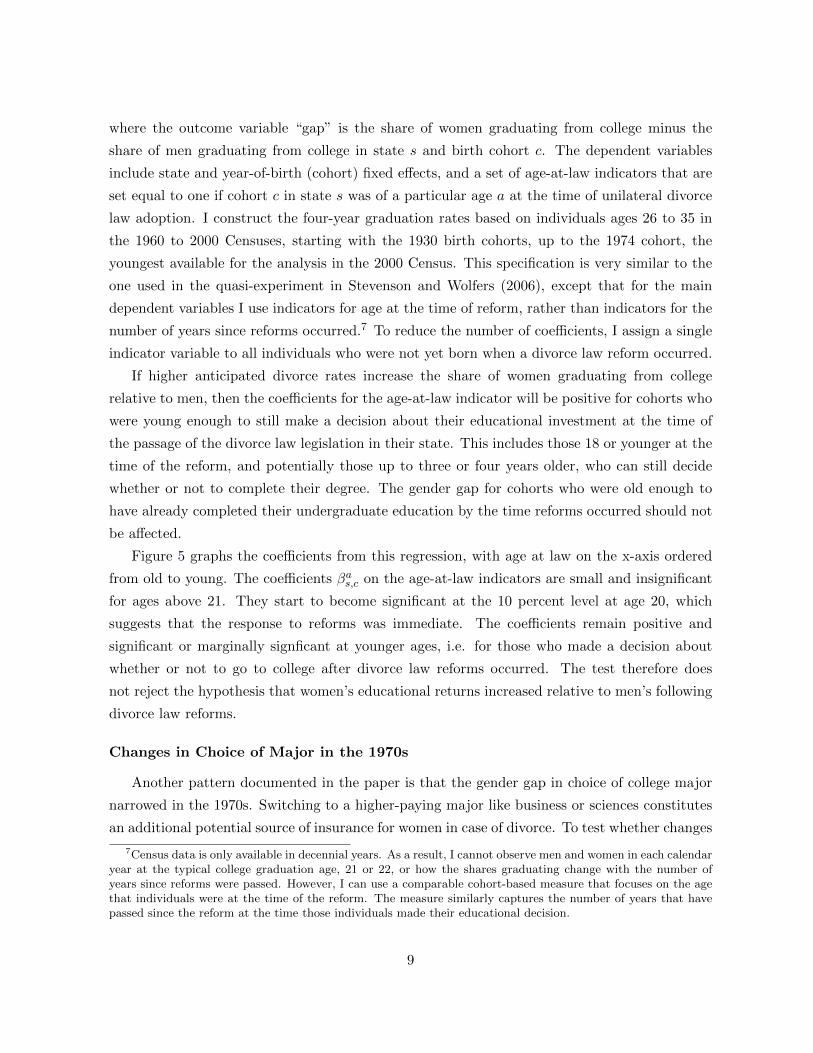
Figure 5 graphs the coefficients from this regression, with age at law on the x-axis ordered

from old to young. The coefficients βas,c on the age-at-law indicators are small and insignificant

for ages above 21. They start to become significant at the 10 percent level at age 20, which

suggests that the response to reforms was immediate. The coefficients remain positive and

significant or marginally signficant at younger ages, i.e. for those who made a decision about

whether or not to go to college after divorce law reforms occurred. The test therefore does

not reject the hypothesis that women’s educational returns increased relative to men’s following

divorce law reforms.

Changes in Choice of Major in the 1970s

Another pattern documented in the paper is that the gender gap in choice of college major

narrowed in the 1970s. Switching to a higher-paying major like business or sciences constitutes

an additional potential source of insurance for women in case of divorce. To test whether changes

7Census data is only available in decennial years. As a result, I cannot observe men and women in each calendaryear at the typical college graduation age, 21 or 22, or how the shares graduating change with the number ofyears since reforms were passed. However, I can use a comparable cohort-based measure that focuses on the agethat individuals were at the time of the reform. The measure similarly captures the number of years that havepassed since the reform at the time those individuals made their educational decision.

9

in divorce laws also contributed to the increase in the relative number of women in these fields,

I conduct a test similar to the previous one. For this purpose, I first classify majors into two

groups – “sciences/business,” and “humanities/all others,” and record the share of men and the

share of women in each cohort who choose science/business majors. Grouping major choices

into these two broadly defined categories allows me to construct a single variable, the share of

individuals choosing a science and business major, which simplifies the reduced form analysis.

Because the Census does not have information on majors, for this particular test I use state-

level data from the Higher Education General Information Survey (HEGIS), which provides data

on undergraduate degrees earned yearly by gender and field between 1965 and 1985. I conduct

a similar test as before, using the following specification:

Gaps,y = α+∑n,s,y

βns,yY earssincelawns,y +

∑s

γs +∑y

λy + εs,y (2)

where the outcome variable is the share of graduating college women who choose a science or

business major in a given year y and state s minus the share of college men who graduate with

such majors. “Years-since-law” is a set of indicators corresponding to the number of years since

the divorce law reform was passed in state s. Because of the small number of observations, I

group the years n for the years-since-law indicator in the following way: -2 to 0, 1 to 3, 4 to 6,

7 to 9, and 10 or more. The first of these indicators allows me to test for a pre-trend, similarly

as in the previous analysis using age at time of divorce law. The omitted category includes all

states that are three or more years away from passing a divorce law reform.

Table 1 reports the coefficients on the years-since-law indicators. As expected, the coefficient

corresponding to zero to two years prior to the divorce law reforms is statistically zero. The

coefficient on the indicator variable corresponding to one to three years is also insignificant.

This contrasts with the results obtained for the gender gap in college attendance, in which the

effect of divorce law reforms was immediate. Only after four years, the effect on the gender

gap in majors becomes statistically significant. The difference between the two results is likely

explained by the fact that it is difficult to switch majors after already completing one or more

years of study. As a result, one would not observe a response in choice of major until at least

four years after the divorce law reform. The coefficient on the indicator corresponding to 7 to 9

years continues to be significant, but at 10 years, the coefficient loses significance.

The results obtained using cross-state variation in the timing of divorce law reforms provide

evidence that both “gender gaps” narrowed following divorce law reforms, suggesting that both

the returns to getting a college education as well as the returns to getting a higher-paying major

increased for women relative to men after the reforms. How large are these effects? The size

of the regression coefficients from the reduced-from analysis suggest that divorce law reforms

10

explain around 13% of the convergence between men and women in graduation rates observed in

the 1970s. The effects on the gender gap in majors are somewhat smaller. However, it is possible

that the size of the coefficients understates the real effect. Firstly, individuals’ mobility across

states after graduation introduces substantial measurement error in the analysis. Secondly,

contamination effects may play a role. For example, as more states implement reforms with

time, individuals in states under the old divorce law regime may nevertheless respond to the

nationwide changes, e.g. by anticipating similar reforms in their own state. Both factors would

bias the coefficients downward. In Section 5, I estimate using the model an alternative measure

of the effect of divorce laws on college attendance and compare it to the reduced-form estimates.

Persistent Differences in Choice of Major Since the Mid-1980s

The persistent difference in the choice of undergraduate major documented in Figure 2 raises

the question why, given their high college attendance rates, women did not converge further with

men along this second margin, or similarly overtake them. Before answering this question, one

potential concern that needs to be addressed is that the patterns in Figure 2 do not account for

the change in the weight of different majors over time, and may thus misrepresent the persistence

of the gender gap in majors. In particular, some traditionally “female” majors like education

became less popular over time, while other majors that were historically “male” and became

more gender-equal, such as business, increased in popularity (NCES (2012)).

To address this, Figure 6 graphs separately the share of men and the share of women choosing

different categories of majors over time using NCES data. For simplicity, majors are aggregated,

as in the previous subsection, into two categories: science/business and humanities/other. Figure

6 documents two patterns. First, for both men and women the popularity of science/business

majors as a share of all degrees increased in the 1970s, although the increase was larger for

women, meaning that men and women converged during this period. The share of women

majoring in science/business quadrupled from about 10% in 1970 to almost 40% by the the

mid-1980s. Men’s share increased from roughly 50% to a peak of 68% in 1986, before declining

slightly. Secondly, after the mid-1980s the share of men and women choosing a science or business

degree has remained roughly stable, at about 60% for men and 36% for women. This implies

that convergence virtually ceased after the mid-1980s, as was also documented in Figure 2.8

To analyze whether persistent differences in choice of major are driven by gender differences

8The period of interest in this paper is from 1960 to 2010, but NCES data on these measures begins in 1970. Tocheck whether substantial changes occurred prior to 1970, I use the National Survey of College Graduates, whichhas data for cohorts that graduated between 1960 and 1970. In the NSCG the share of women graduating with ascience/business degree between 1960 and 1970 was almost constant, 15% in 1960 and 16% in 1970. However, theNSCG sample overestimates the share graduating in 1970 relative to the NCES data (10%), which includes theentire population of graduation college students. The NSCG also overestimates the share of men with a scienceor business degree. It records a temporary decline in the measure over that decade, from 61% to 55%.

11

in wage premiums by field, Table 2 compares the premiums for men and women with different

undergraduate majors in 1993, 2003, and 2010, the three waves of the National Survey of

College Graduates. The premiums are the coefficients from a regression of log income for full-

time workers on a set of dummy variables corresponding to each undergraduate major. The

omitted category is a major in the arts and humanities. The coefficient is interpreted to be the

“additional” income in log points that individuals in a given major receive, relative to those in

the baseline humanities major.

Table 2 documents two main findings. Firstly, it documents that men’s and women’s returns

to different college majors exhibit similar patterns. The lowest-paying major for both men and

women is education, which pays at least 7% less than a humanities degree in all years, although

this difference is not statistically significant in 2010. For both men and women, a social sciences

degree provides a very similar return to a humanities degree. Among non-science and non-

business majors, degrees in health support fields stand out for their high return, with similar

premiums for men and women that range from 14 to 19 log points (13-17%) in 1993 and 2003,

and with even higher returns in 2010.9,10

The second finding documented in Table 2 is that full-time workers with science, engineering

and business majors have high premiums relative to those with humanities, education, or social

science degrees. Business and math/science majors are associated with an additional return of

between 16 and 26 log points (15-23%) for men, and 14 to 20 log points (13-18%) for women.

Degrees in engineering and technology are the highest-paying degrees. The additional premium

for men is 31-36 log points (27-30%), and for women it is even higher, 38-45 log points (32-37%).

To summarize, these patterns together imply that with the notable exception of nurs-

ing/health support, a field that represents about 11% of degrees for women, women are sub-

stantially more likely than men to select majors that have on average low expected returns.

Majors and Flexibility

If women frequently choose lower-paying majors, some other characteristic of these majors

should compensate them for the lower return. The popularity of degrees like education and

nursing among women suggests that one such possible characteristic is the degree of “flexibility”

offered in occupations associated with different majors. I define “flexibility” by high availability

of part-time or part-year work and by low wage penalties in case of a temporary absence from

the workforce or reduction of weekly hours worked. If women value such flexibility more than

9Majors classified under “health” include nursing degrees and other programs related to health support oc-cupations. Bio-med and pre-med majors, which prepare students for medical research or practice, are classifiedunder “sciences.” See Appendix A for additional details.

10The substantial increase in the return to a health major from 2003 to 2010 could partly be explained by thehealth industry’s strong performance relative to other industries during the recession (Wood (2011)).

12

men, this may help explain observed differences in choice of major.

Before analyzing how majors differ along this margin, I provide evidence first for why college-

educated women today may value such flexibility. Figure 7 graphs the share of college-educated

men and women employed and the share working full-time at each age between 22 and 50.

The data is for the year 2000, but identical patterns hold in 1990 and 2010.11 Figure 7 shows

that men and women exhibit similar rates of employment and full-time work immediately after

college graduation. However, college women begin to drop their employment rates and their

hours worked in their late twenties, and continue to do so through their child-bearing years.

Women’s overall employment and full-time employment rates reach their lowest point in their

mid-30s. At age 35, 60% of college-educated women work full-time, compared to more than 90%

of college-educated men. Afterwards, women gradually increase their labor supply again. As

Panel B shows, these large reductions in labor supply over the lifetime are primarily driven by

women with young children under the age of 6 in the household.

In the rest of the section, I examine whether labor supply patterns differ substantially by

the type of major chosen and its associated occupations. I analyze the following measures of

flexibility in labor supply, focusing on women with young children: part-time work, employment

rates, and annual hours worked, where the latter is a summary composite of the first two

measures. After documenting labor supply patterns, I analyze wage penalties by major and

occupation group for reductions in labor supply.

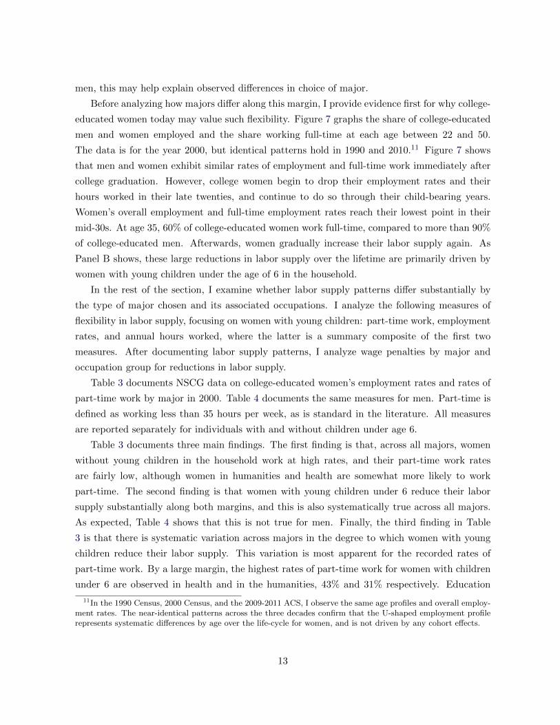
Table 3 documents NSCG data on college-educated women’s employment rates and rates of

part-time work by major in 2000. Table 4 documents the same measures for men. Part-time is

defined as working less than 35 hours per week, as is standard in the literature. All measures

are reported separately for individuals with and without children under age 6.

Table 3 documents three main findings. The first finding is that, across all majors, women

without young children in the household work at high rates, and their part-time work rates

are fairly low, although women in humanities and health are somewhat more likely to work

part-time. The second finding is that women with young children under 6 reduce their labor

supply substantially along both margins, and this is also systematically true across all majors.

As expected, Table 4 shows that this is not true for men. Finally, the third finding in Table

3 is that there is systematic variation across majors in the degree to which women with young

children reduce their labor supply. This variation is most apparent for the recorded rates of

part-time work. By a large margin, the highest rates of part-time work for women with children

under 6 are observed in health and in the humanities, 43% and 31% respectively. Education

11In the 1990 Census, 2000 Census, and the 2009-2011 ACS, I observe the same age profiles and overall employ-ment rates. The near-identical patterns across the three decades confirm that the U-shaped employment profilerepresents systematic differences by age over the life-cycle for women, and is not driven by any cohort effects.

13

majors stand out for their low part-time work rates (20%) among non-science, non-business

majors; however, the part-time work measure does not capture the part-year nature of work in

teaching professions.12 Differences in employment rates across majors for women with young

children are somewhat less clearcut, but suggest that women in science and engineering have

fairly high employment rates, relative to most other majors. Interestingly, women with young

children who are health majors have even higher employment rates than engineers with young

children; however, this appears to be be driven by the high availability of part-time work in the

health field.

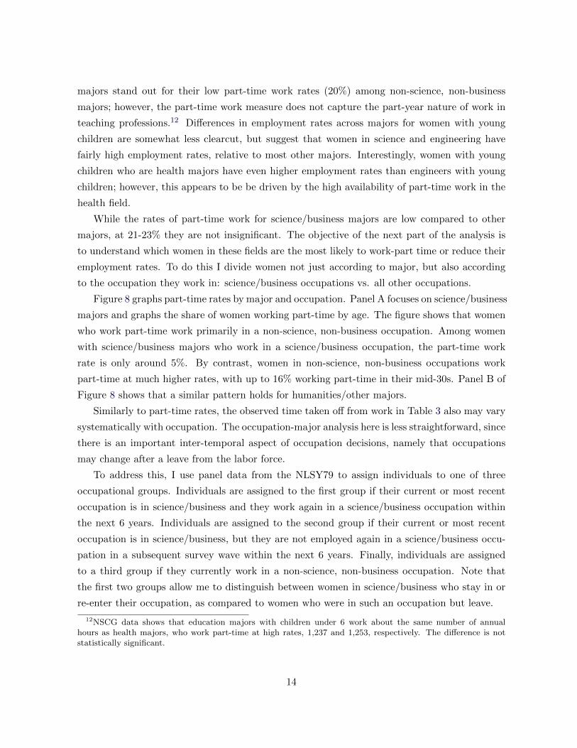
While the rates of part-time work for science/business majors are low compared to other

majors, at 21-23% they are not insignificant. The objective of the next part of the analysis is

to understand which women in these fields are the most likely to work-part time or reduce their

employment rates. To do this I divide women not just according to major, but also according

to the occupation they work in: science/business occupations vs. all other occupations.

Figure 8 graphs part-time rates by major and occupation. Panel A focuses on science/business

majors and graphs the share of women working part-time by age. The figure shows that women

who work part-time work primarily in a non-science, non-business occupation. Among women

with science/business majors who work in a science/business occupation, the part-time work

rate is only around 5%. By contrast, women in non-science, non-business occupations work

part-time at much higher rates, with up to 16% working part-time in their mid-30s. Panel B of

Figure 8 shows that a similar pattern holds for humanities/other majors.

Similarly to part-time rates, the observed time taken off from work in Table 3 also may vary

systematically with occupation. The occupation-major analysis here is less straightforward, since

there is an important inter-temporal aspect of occupation decisions, namely that occupations

may change after a leave from the labor force.

To address this, I use panel data from the NLSY79 to assign individuals to one of three

occupational groups. Individuals are assigned to the first group if their current or most recent

occupation is in science/business and they work again in a science/business occupation within

the next 6 years. Individuals are assigned to the second group if their current or most recent

occupation is in science/business, but they are not employed again in a science/business occu-

pation in a subsequent survey wave within the next 6 years. Finally, individuals are assigned

to a third group if they currently work in a non-science, non-business occupation. Note that

the first two groups allow me to distinguish between women in science/business who stay in or

re-enter their occupation, as compared to women who were in such an occupation but leave.

12NSCG data shows that education majors with children under 6 work about the same number of annualhours as health majors, who work part-time at high rates, 1,237 and 1,253, respectively. The difference is notstatistically significant.

14

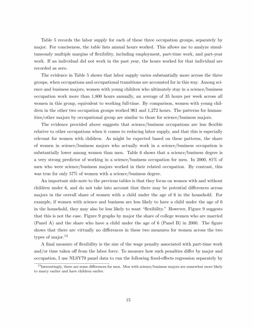
Table 5 records the labor supply for each of these three occupation groups, separately by

major. For conciseness, the table lists annual hours worked. This allows me to analyze simul-

taneously multiple margins of flexibility, including employment, part-time work, and part-year

work. If an individual did not work in the past year, the hours worked for that individual are

recorded as zero.

The evidence in Table 5 shows that labor supply varies substantially more across the three

groups, when occupations and occupational transitions are accounted for in this way. Among sci-

ence and business majors, women with young children who ultimately stay in a science/business

occupation work more than 1,800 hours annually, an average of 35 hours per week across all

women in this group, equivalent to working full-time. By comparison, women with young chil-

dren in the other two occupation groups worked 961 and 1,272 hours. The patterns for human-

ities/other majors by occupational group are similar to those for science/business majors.

The evidence provided above suggests that science/business occupations are less flexible

relative to other occupations when it comes to reducing labor supply, and that this is especially

relevant for women with children. As might be expected based on these patterns, the share

of women in science/business majors who actually work in a science/business occupation is

substantially lower among women than men. Table 6 shows that a science/business degree is

a very strong predictor of working in a science/business occupation for men. In 2000, 81% of

men who were science/business majors worked in their related occupation. By contrast, this

was true for only 57% of women with a science/business degree.

An important side-note to the previous tables is that they focus on women with and without

children under 6, and do not take into account that there may be potential differences across

majors in the overall share of women with a child under the age of 6 in the household. For

example, if women with science and business are less likely to have a child under the age of 6

in the household, they may also be less likely to want “flexibility.” However, Figure 9 suggests

that this is not the case. Figure 9 graphs by major the share of college women who are married

(Panel A) and the share who have a child under the age of 6 (Panel B) in 2000. The figure

shows that there are virtually no differences in these two measures for women across the two

types of major.13

A final measure of flexibility is the size of the wage penalty associated with part-time work

and/or time taken off from the labor force. To measure how such penalties differ by major and

occupation, I use NLSY79 panel data to run the following fixed-effects regression separately by

13Interestingly, there are some differences for men. Men with science/business majors are somewhat more likelyto marry earlier and have children earlier.

15

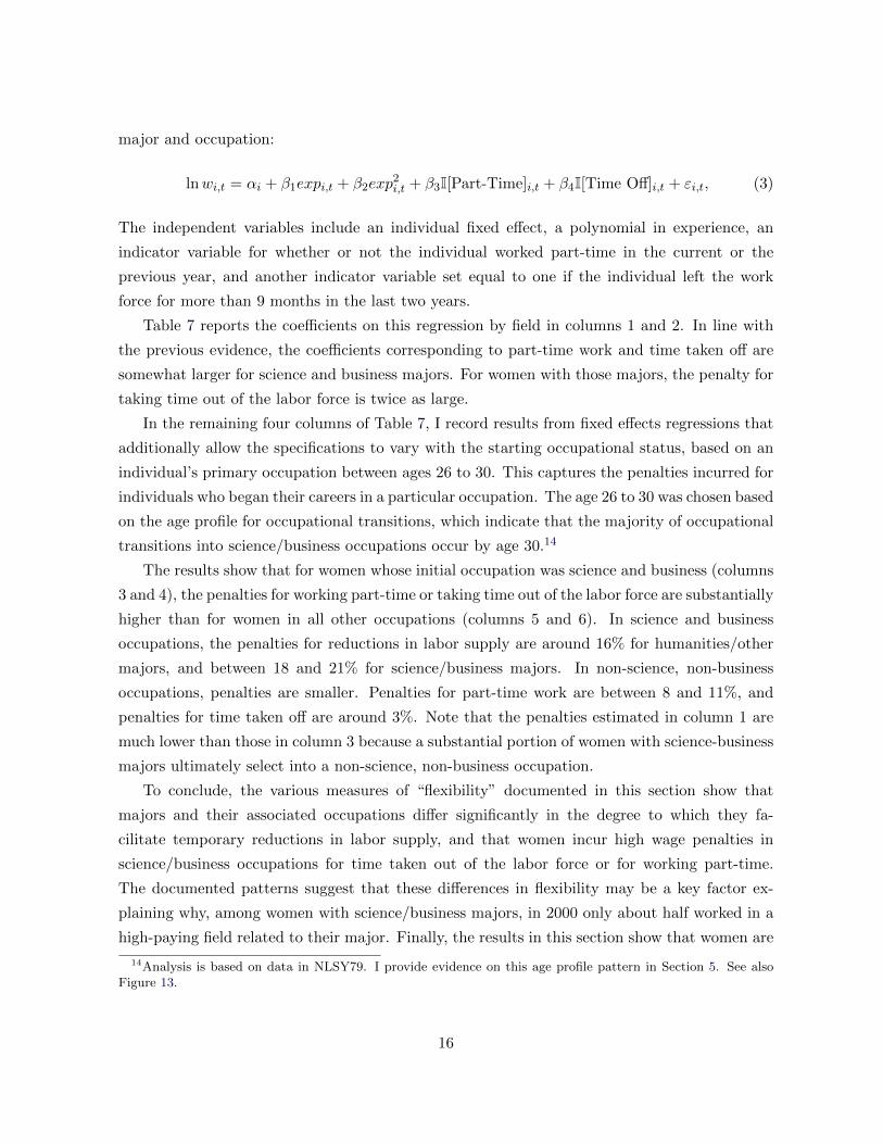
major and occupation:

lnwi,t = αi + β1expi,t + β2exp2i,t + β3I[Part-Time]i,t + β4I[Time Off]i,t + εi,t, (3)

The independent variables include an individual fixed effect, a polynomial in experience, an

indicator variable for whether or not the individual worked part-time in the current or the

previous year, and another indicator variable set equal to one if the individual left the work

force for more than 9 months in the last two years.

Table 7 reports the coefficients on this regression by field in columns 1 and 2. In line with

the previous evidence, the coefficients corresponding to part-time work and time taken off are

somewhat larger for science and business majors. For women with those majors, the penalty for

taking time out of the labor force is twice as large.

In the remaining four columns of Table 7, I record results from fixed effects regressions that

additionally allow the specifications to vary with the starting occupational status, based on an

individual’s primary occupation between ages 26 to 30. This captures the penalties incurred for

individuals who began their careers in a particular occupation. The age 26 to 30 was chosen based

on the age profile for occupational transitions, which indicate that the majority of occupational

transitions into science/business occupations occur by age 30.14

The results show that for women whose initial occupation was science and business (columns

3 and 4), the penalties for working part-time or taking time out of the labor force are substantially

higher than for women in all other occupations (columns 5 and 6). In science and business

occupations, the penalties for reductions in labor supply are around 16% for humanities/other

majors, and between 18 and 21% for science/business majors. In non-science, non-business

occupations, penalties are smaller. Penalties for part-time work are between 8 and 11%, and

penalties for time taken off are around 3%. Note that the penalties estimated in column 1 are

much lower than those in column 3 because a substantial portion of women with science-business

majors ultimately select into a non-science, non-business occupation.

To conclude, the various measures of “flexibility” documented in this section show that

majors and their associated occupations differ significantly in the degree to which they fa-

cilitate temporary reductions in labor supply, and that women incur high wage penalties in

science/business occupations for time taken out of the labor force or for working part-time.

The documented patterns suggest that these differences in flexibility may be a key factor ex-

plaining why, among women with science/business majors, in 2000 only about half worked in a

high-paying field related to their major. Finally, the results in this section show that women are

14Analysis is based on data in NLSY79. I provide evidence on this age profile pattern in Section 5. See alsoFigure 13.

16

more than 1.5 times as likely to select majors that are associated with occupations with low wage

penalties for reductions in labor supply, and higher availability of flexible work arrangements,

like part-time work.

3 Model

In this section, I develop and estimate a lifetime model of individual decisions that can capture

the empirical features around marriage and divorce, labor supply, and education described in

the previous section. There are several reasons why such a model is useful. Firstly, with a

model it is possible to analyze cumulative processes and interactions, such as the increase in

divorce rates over time or changes in labor supply, which can be results of as well as the drivers

of educational investment decisions. Using a model, it is possible to account explicitly for the

fact that marriage, labor supply, and education decisions are jointly made, and that a change in

the choice about one of these factors affects the optimal decision about all the others. Secondly,

it is possible to analyze the relative importance of changes in the wage structure and changes

in the marriage market in generating the observed dynamics in educational choices. Finally,

it is possible to perform policy simulation exercises. Because policies that seek to increase the

share of science-technology majors have been recently proposed, performing such simulations

to analyze their potential effects is particularly useful. One policy that has received recent

media attention is a proposal to charge differential tuition for science and non-science majors at

state universities in Florida (Alvarez (2012)). Additionally, policies and practices around work-

family flexibility receive periodic media attention.15 Because the model in this paper explicitly

considers household labor supply, marriage, and household specialization, it is well-suited for

analyzing the channels through which such policies may affect educational choices.

In this section, I first provide an overview of the main features of the model and the set

of dynamics that the model can capture. I then provide details about each component of the

model, and finally about the decisions of individuals in each period.

3.1 Overview of the Model

The model is a dynamic individual lifetime model, where individuals live for T periods, starting

at age 18. I first outline the main idea of the model and its four most important features.

There are three phases of life: education, working life, and retirement. The first two phases,

education and working life, are the main focus of the model.

In the first phase, young individuals decide whether to make an educational investment. If

15For two recent examples, see Rampbell (2013) and Bernard (2013).

17

they do not go to college, they begin the working phase of their life. Education choices cannot be

changed once the working life phase begins. If they decide to go to college, they choose between

two majors. One major is associated with a high-return, high skill depreciation occupation. In

this occupation, there is a high wage penalty for temporary absences from the workforce and

for part-time work. The other major is associated with a lower-return, lower skill depreciation

occupation. These differences in characteristics between the majors are designed to correspond

to differences between science/business majors vs. humanities/other majors documented in the

empirical section. This is the first key feature of the model.

In the second, working life phase individuals make decisions about marriage and divorce. If

single, an individual meets a potential partner with some probability and decides whether or

not to marry; if married, he or she decides whether to remain married or to divorce. Couples

cooperate when making decisions but cannot commit to future allocations of resources. Divorce

occurs when no reallocation of resources within the household can make both individuals better

off married than single. This lack of full commitment allows for divorces to occur in the model

as they do in the data and it is the second important feature of the model.

In every period of the second phase individuals also make decisions about labor supply, which

is allocated to market, home production, and leisure. During the working life phase, there are

three sources of uncertainty–wage shocks, marital match quality shocks, and fertility shocks.

Fertility is modeled as an exogenous process, conditional on marital status and age. After a

fertility shock, the presence of children has the effect of increasing the productivity of labor in

home production, which allows the model to capture the large increase in hours allocated to

home production and child care observed in the data after childbirth. This aspect of the model

also enables me to capture potential gains to partial or full specialization in market and home

production for married couples. This is the the third important feature of the model.

Finally, the model not only follows individuals from a given cohort over the lifecourse, but

also simulates different cohorts over time. There are two main sources of variation across co-

horts, assumed to be exogenous. One is the distribution of entry wages, conditional on sex and

education. The other is the cost of divorce. In particular, there is a one-time drop in the cost

of divorce in 1970 corresponding to the beginning of divorce law reforms. This captures that

divorce became substantially easier after the reforms, the final important feature in the model.

Young individuals in each cohort take into account the change in divorce laws when they form

expectations about their own future probability of divorce.

The four outlined features make up the structure that generates the key dynamics of the

model, over the lifetime as well as across cohorts. In each cohort, individuals face competing

considerations. In some periods, especially when there are young children in the household,

married individuals may find it optimal to specialize by having one of the spouses commit

18

substantial time to home production, by partly or fully reducing the labor supplied to the

market. It will often, but not always, be optimal for the woman to be the one to reduce her

labor supply, since she draws on average from a lower wage distribution. On the other hand,

working in the labor market increases human capital, and thus future wages. The spouse that

reduces labor supply reduces his or her future labor market prospects. Moreover, depending

on current occupation, the spouse who reduces labor supply may incur a high additional wage

penalty, in addition to the wage losses from foregone experience. Individuals’ decisions about

labor supply and education will reflect these competing considerations. Changes in the wage

structure and in marriage and divorce patterns over time will in turn affect those considerations.

With this overall idea of the model in mind, we now turn to the specific modeling choices. I

first provide details about each component of the model, and then characterize the decisions of

individuals in each period.

3.2 Preferences

Individuals derive utility from consumption c, leisure l and a household-produced good Q. Q is

a privately consumed good (Qi) if individual i is single, and it is consumed as a shared public

good (Q) if the individual is married. Couples additionally derive utility from match quality θ.

Preferences are separable across time and across states of the world. In each period, the utility

function is assumed to be separable in (cit, lit) and Qt to simplify the estimation, and to take the

following form:

uisingle = u(cit, lit) +A logQit uimarried = u(cit, l

it) +A logQt + θt.

Following empirical evidence from Attanasio and Weber (1995) and Meghir and Weber (1996)

that individual preferences are not separable in consumption and leisure, I assume the following

functional form for the subutility u(cit, lit):

u(cit, lit) =

(citalit1−a

)1−σ

1− σ, σ > 0, 0 < a < 1

The last component of utility is match quality. Match quality is assumed to follow a random

walk stochastic process, where

θt = θt−1 + zt, zt ∼ N(0, σz).

19

3.3 Household Technology

The good Qt is produced within the household using market good mt, labor input dt, and

number of children nt. To keep the computation simple, I assume a form for the household good

production function that is log linear in the inputs:

log(Qt) = α1,t log dt + α2 logmt + α3 log (1 + nt), (4)

where dt = dit if the individual is single, and dt = dit + djt , i.e. the sum of the husband’s and the

wife’s labor allocated to home good production, if the individual is married. Note that this is

equivalent to assuming that the husband’s and wife’s labor inputs are perfectly substitutable.

Children increase the production of the household good directly, to capture that one of the

additional potential returns to marriage is having a family with children.

To introduce heterogeneity in the productivity of labor in home production, α1,t is allowed

to differ over time and across households. Specifically, the parameter α1,t can take one of five

values, which will be estimated using time use data on hours allocated to home production

and child care: a value for households without children; two values for households with young

children, one for each of two educational levels (high school or college); and two values for

households with older children, one for each educational level (high school or college). Labor

productivity in home production does not depend on major.16

By allowing α1,t to vary with the age and presence of children, it is possible to capture the

large difference in labor allocated to home production between households without children,

households with children under the age of six, and households with children over the age of

six. The reason the parameter is allowed to vary additionally with education in households with

children is that it allows the model to capture the systematic differences in time allocated to child

care by educational attainment. For example, Guryan, Hurst, and Kearney (2008) document

that college-educated women allocate more hours both to the labor market and to child care.

3.4 Fertility Process

Children are born according to an exogenous fertility process that depends on marital status,

age, and the current number of children. A fertility shock can occur if an individual is married

and of childbearing age, which in the model is set to 38 or below. The fertility hazard rates are

estimated externally.

16Note that spouses’ labor in home production is substitutable. In married households, I have to choose whichspouse’s education will be used to determine the household’s α1,t parameter. I assume the education of the womandetermines the productivity parameter. I assign productivity based on the wife’s education because women tendto supply the majority of labor in home production in the data (ATUS, 2003). This is not a restrictive assumptionsince spouses have the same educational attainment in the majority of couples in the data.

20

3.5 Wage Process and Human Capital

Wages in the model depend on education, current occupation, and accumulated experience. I

provide information about each of these factors first, and at the end of the subsection I describe

in detail how they enter into the wage process.

3.5.1 Education and Occupation

There are three educational choices: (1) high school only; (2) college with a major “L” that

provides a premium in low-return, low skill-depreciation occupations; and (3) college with major

“H” that provides a premium in high-return, high skill-depreciation occupations. I refer to the

occupations described respectively as “L”-type and “H”-type. The two majors (L,H) capture

the differences in the data documented in the previous section between science/business vs.

humanities/other majors. College individuals then choose whether to work in a science/business

occupation (H) or all other occupations (L).

I make a simplifying assumption that individuals with a high school education all work in the

same L-type occupation. In the NLSY79, the share of individuals without a college education

who work in a H-type (science/business) occupation is less than 8%.

3.5.2 Experience

Individuals who work the equivalent of at least 500 annual hours in a given period accumulate

one additional period of experience. Experience in the model is occupation-specific. If an

individual decides to switch occupations, he or she loses his or her accumulated experience, and

must begin accumulating experience again from zero. Though it would be preferable to keep

track of experience accumulated in each occupation, I make this assumption to keep the model

tractable. In the NLSY79, I observe that most occupational switches occur before the age of

28, that is before individuals have had the opportunity to accumulate substantial experience,

which suggests that the assumption is not highly restrictive. The share of men and women who

switch between the two categories of occupations more than once after age 30 is around 12%.

3.5.3 Part-Time Work and Time Out of the Labor Force

Working a minimum number of hours in the model matters for accumulating experience. Ad-

ditionally, the number of hours worked in a given period is important because it determines

whether or not an individual will incur a wage penalty for working less than full-time, full-year.

I do not model separately the decision to work part-time and the decision to take time out of the

labor force. In the model, only the total number of hours worked in a given period is relevant.

21

If the amount of labor supplied in the current period is equivalent to less than 35 hours per

week, the individual incurs a wage penalty in the following period. The size of the wage penalty

depends on whether the individual works in a L- or H-type occupation.

3.5.4 Wage process

Individuals draw from wage processes specific to their sex, occupation, and education. I will

describe first the wage process for individuals with a high school education, and then describe

the process for individuals with a college education.

Individuals with a high school education draw a wage every period for only one possible

occupation. This means that there are a total of two wage processes to be estimated for high

school individuals, one for women and one for men. An individual of gender k, experience expt,

and number of hours ht−1 worked in the previous period draws a wage from the following process:

lnwt = βk,HS0 + βk,HS1 expt + βk,HS2 exp2t + βk,HS3 I(ht−1 < h) + εk,HSt , (5)

εk,HSt ∼ N(0, σεk,HS )

where h is equivalent to the minimum hours worked for a full-time, full-year worker. The

coefficient β3 on the indicator function I(ht−1 < h) is the current-period wage penalty incurred

for working less than full time in the previous period. If the wage drawn in a particular period

falls below a value equivalent to the minimum wage, the effective wage is zero and the individual

is not employed. Otherwise, the individual may work at hourly wage wt.

The structure of the wage process for individuals with a college education is similar, except

that college-educated individuals draw wages for up to two occupations, H and L. An individual

who enters the period having last worked in a particular occupation will draw a wage from that

occupation with probability one. Additionally, with probability η the individual draws a wage

from the second occupation and can choose whether or not to switch occupations. Specifically,

an individual of gender k with a given major M who enters the period having last worked in

occupation qt−1 draws the following wage for occupation q = qt−1:

lnwt = βk,M,q0 + βk,M,q

1 expt + βk,M,q2 exp2t + βk,M,q

3 I(ht−1 < h) + εk,M,qt , (6)

εk,M,qt ∼ N(0, σεk,M,q)

The coefficients are indexed by k and M because the wage processes are estimated separately

by sex and major.

If the individual draws a second wage for the other occupation r 6= qt−1, the wage is charac-

22

terized by

lnwt = βs,M,r0 + βs,M,r

3 I(ht−1 < h) + εs,M,rt , (7)

εs,M,rt ∼ N(0, σεs,M,r)

since the individual loses his or her accumulated experience after switching. As before, the

coefficient on I(ht−1 < h) is a penalty for working less than full-time. To reflect the data, this

estimated penalty will be high in H-type occupations, and lower in L-type occupations.

Allowing for occupational choices in addition to educational choices in the model is important

for two reasons. Firstly, it allows the model to capture the fact that only a small share of men

but almost half of women with a science/business major work in non-science, non-business

occupations, as documented in the previous section.17 This difference in occupational choices

strongly affects the return to a science/business major for women relative to men, and the model

should be able to capture this feature of the data. The second reason is that variation in wages

across occupations is greater than the variation in wages within occupations in the data. This

suggests that accounting for the actual occupational choice is important.

In the data individuals that have majors that correspond to their occupation on average

earn more in that occupation than those in the occupation who have a different major. These

differences observed in the data will be reflected in the estimated wage process parameters.

Estimation of the wage process parameters will be discussed in detail in Section 4.

3.6 Educational Costs

Individuals who choose to go to college incur a tuition cost τ , which is deducted from their assets.

Individuals also have major-specific utility costs CiL and CiH , interpreted to be the individual’s

ability or effort costs for completing a particular major. This is the only source of unobserved

heterogeneity across individuals. Individuals draw CiL and CiH from normal distributions char-

acterized by parameters (µL, σL) and (µH , σH). Men and women have the same distributions of

effort costs. Educational decisions can only be made in the first period.

3.7 Cost of Divorce

If a married couple wishes to divorce, each individual incurs a one-time utility cost Kt. The

cost takes two possible values. K0 corresponds to the cost of divorce before no-fault, unilateral

divorce law reforms. K1 corresponds to the cost of divorce after such reforms. The change from

K0 to K1 occurs in 1970, corresponding to the timing of the start of divorce law reforms. I

assume that cohorts did not anticipate the change. The change in Kt can be interpreted as

17Similarly, some men and women with humanities/other majors work science/business occupations.

23

a change in the amount of effort required to secure a divorce, in line with historical evidence.

For example, prior to reforms individuals and/or couples resorted in many cases to perjury or

providing exaggerated or false testimony to provide fault-based grounds (Herbert (1988)).

3.8 Individual Decisions

With all the main components of the model laid out, I now describe households’ decisions,

starting with the working life stage. Afterwards, I describe the retirement stage, which is a

simplified version of the household’s problem during the working life stage. Finally, after the

description of what happens over the lifecourse, I discuss the educational decision that takes

place in the first period. It is best left for last to discuss this decision because it requires

knowledge of the expected stream of lifetime utility from each educational choice.

During the working life phase, individuals enter every period t either single or married,

and make a decision about their marital status that period. Shocks to wage, match quality and

fertility are realized at the beginning of the period, before any decisions are made. An individual

who has completed his or her education and enters the period as single meets a potential spouse j

with probability one, and draws a match quality θt. This individual must now choose whether to

stay single or to marry the potential partner, and to make this decision, he or she must compare

the value of staying single with the value of marrying the potential partner. Similarly, an

individual who enters as married makes a decision between staying married or getting divorced,

and to do that he or she compares the values of those two options.

I will first describe the problem of an individual who enters the period as married. If the

couple to whom the individual belongs decides to divorce, he or she will experience the value of

being single, V i,St , that can be computed as follows. The individual will choose the levels of own

consumption cit, labor supplied to the market hit, labor supplied to home production dit, leisure

lit, savings sit, and the amount of the market good mit devoted to home good production that

maximizes his or her lifetime expected utility. If an individual receives a wage draw from more

than one occupation, the individual additionally chooses which occupation to work in, qit. The

value of staying single for the individual is therefore equal to

V i,St = max

cit,lit,m

it,d

it,h

it,q

it,s

it+1

ui(cit, lit, Q

it) + βE[V i

t+1(ωt+1|ωt)]

24

s.t. cit +mit + pkn

it = with

it +Rsit − sit+1 (Budget Constraint)

Qit = F i(mit, d

it, n

it) (HH Good)

wi,q=qt−1

t = Gi(edi, expit, hit−1, ε

it) (Wage I)

wi,r 6=qt−1

t = Gi(edi, hit−1, εit) (Wage II)

hit + dit + lit = T (Time Constraint)

where ωt is the set of state variables in period t, and E[V it+1(ωt+1|ωt)] is the expected value

function of the individual when he or she enters period t+ 1 as single.

Now consider the value of staying married, V i,Mt , for the same individual that enters the

period as married. The value V i,Mt is determined by modeling the decisions of the married

household as a Pareto problem with participation constraints. In determining V i,Mt , I fol-

low the literature on decisions with limited commitment (e.g. Marcet and Marimon (1992,

1998), Ligon et al. 2000), and in particular its application to models of intra-household al-

location (Mazzocco (2007)). This literature shows that the Pareto problem with participa-

tion constraints can be solved in two steps. In the first step, the household solves the un-

constrained problem. This means that in period t the married couple chooses the vector

zt = {cit, cjt , l

it, l

jt , d

it, d

jt , h

it, h

jt , q

it, q

jt ,mt, st+1} to solve the following Pareto problem, with weights

µt and (1− µt):

maxzt

µt[ui(cit, l

it, Qt, θt) + βE[V i

t+1(ωt+1|ωt)]] + (1− µt)[uj(cjt , ljt , Qt, θt) + βE[V j

t+1(ωt+1|ωt)]]

s.t. cit + cjt +mt + pknt = withit + wjth

jt +Rst − st+1 (Budget Constraint)

Qt = F i(mt, dit, d

jt , nt) (HH Good)

wk,q=qt−1

t = G(edk, expkt , hkt−1, εt), k = i, j (Wage I)

wk,r 6=qt−1

t = G(edk, hit−1, εt), k = i, j (Wage II)

hkt + dkt + lkt = T , k = i, j (Time Constraint)

When the optimal solution z∗ to the unconstrained problem is determined, one can calculate

V ∗k,Mt (z∗) = ui(c∗it , l∗it , Q

∗it ) + βE[V ∗it+1(ωt+1|ωt)], k = i, j

i.e. the value of being married for spouse k at the current Pareto weights µt and (1− µt).

25

In the second step, one can then check that the solution satisfies both individuals’ partici-

pation constraints. Recall that if the couple divorces, each partner incurs the one-time utility

cost Kt. Hence, the constraints for individuals that entered the period married take the form

V ∗k,Mt ≥ V k,St −Kt, k = i, j

If the participation constraints for both partners are satisfied at V ∗k,Mt (z∗), the allocations

determined in the first stage are the final allocations and the couple stays married. In that case,

V k,Mt = V ∗k,Mt (z∗), V k

t = V k,Mt , k = i, j.

If both constraints are violated, the marriage generates no surplus and the couple divorces.

Finally, if only one of the constraints is satisfied for the married couple, there is potential for

a renegotiation. I use the result from Ligon, Thomas, and Worrall (2002) that in the optimal

solution, the constrained individual’s Pareto weight is increased so that the individual is exactly

indifferent between staying in the marriage and leaving it. Suppose under this new weight

corresponding to µ̃t, the solution to the household’s maximization problem is z̃∗. If the other

spouse’s participation constraint is still satisfied under the solution z̃∗, then the couple stays

married. If not, then there is no value of the Pareto weight that simultaneously satisfies the

participation constraints of both partners, and the individuals divorce. In that case, V kt is the

value of being divorced, V k,St −Kt, for k = i, j. For married couples, µt constitutes an additional

state variable.

Individuals who enter the period as single calculate the value of being single and the value

of being married to a potential partner in almost the exact same fashion. However, there are no

participation constraints for individuals who enter the period as single. They simply compare

their value of being single and their value of being married. If the latter is higher for both

individuals, they marry. The initial Pareto weights for a couple that marries are determined

using symmetric Nash bargainig.

The problem of the household in retirement is a simpler version of the household’s problem

in the working life. The only decisions in retirement are about consumption, leisure, savings,

and the amount of time and market good allocated to home production. In the final period,

all resources are used and savings are equal to zero. Because retirement decisions are not the

focus of the model, I simplify the problem by not allowing individuals to divorce or marry in

retirement. As a result, individuals who enter retirement married simply solve the married

household’s unconstrained problem, with the Pareto weights fixed throughout retirement.

Now that I have described the decisions that occur over the lifetime, I can describe the educa-

26

tional decision that takes place in the first period. The decision takes into account expectations

about marriage, divorce, occupational and labor supply choices over the lifetime, conditional on

each educational choice. The expectations at the time of the educational decision about future

lifetime utility from each educational choice is expressed as E[V1|ed]. Additionally, the decision

about education depends on the idiosyncratic utility costs associated with going to college and

choosing major L or H. An individual will choose to go to college if either

E[V1|ed=L]− CiL ≥ E[V1|ed=HS ], or

E[V1|ed=H ]− CiH ≥ E[V1|ed=HS ].

If neither condition holds, the individual does not go to college and begins the working stage of his

or her life. Otherwise, the individual chooses the major that gives him or her the higher return,

max {(E[V1|ed=L]− CiL), (E[V1|ed=H ]− CiH)}. This individual does not make any decisions about

labor supply or marriage for two periods, equivalent to four years in the model. After completing

college, the individual begins the working life stage. It is not possible to change one’s education

after the initial educational decision is made.

4 Estimation

In this section I discuss the simulation and estimation of the model. I first provide additional

details about matching in the marriage market and assumptions about divorce and children,

which are needed to operationalize the model. I then discuss the estimation method.

4.1 Implementation Details for Model Simulation

To be able to simulate the model, I must make additional assumptions which were not discussed

in Section 3 about how individuals meet in the marriage market, about the cost of children in

the household, and about how couples split wealth and child custody after divorce. I describe

these assumptions and the data patterns they are founded on below.

Individuals in the model draw potential partners from their own cohort. To capture that

more than 80% of individuals marry someone with the same educational attainment (IPUMS

USA, 2000), I introduce an assumption about how individuals meet in the marriage market.18 I

assume that the probability each period that a single individual draws a potential partner with

the same educational attainment (high school or college) is equal to pm, which is estimated in

18In 2000, 80% of married individuals between ages 18 and 60 were married to a spouse with same educationalattainment as their own, where the two categories of attainment are defined as “college” and “less than college.”Note that the share did not change substantially over time. In 1970, 1980, and 1990, the share of individuals witha spouse that has the same education were 87.7%, 84.2%, and 81.7%, respectively.

27

the model. Conditional on drawing a college-educated partner, the probability that the partner

has a particular major simply corresponds to the share of individuals of that sex who choose

that major.

Spouses in the model pool their savings after marrying. If a married household has children,

the household pays a cost per child pk equivalent to $6000 per year for the first child and

$4500 for subsequent children, as estimated from the Consumer Expenditure Survey.19 If a

couple divorces, the individuals split their total savings evenly, to reflect available data on

asset allocations after divorce. Additionally, I must choose a rule that determines how couples

split custody and financial responsibilities for children after divorce. According to the Census

Bureau, women represent 85% of all custodial parents. About 45% of custodial mothers receive

any kind of child support, and the average amount received for these women is $3,800 (Grail

(2002)). Given the cost of children pk, the received child support payments cover about 14.3%

of the child expenditures in a divorced household with two children. As a result, I assume that

divorced women are responsible for the majority of financial costs for the children, 85%, while

divorced men are responsible for the remainder.

To simplify the simulation of the model, I assume that if a divorced woman with children

remarries, the new household treats the children as its own. If a divorced father re-marries, he

does not bring any children into the new household, and I cease keeping track of children from

his previous marriage. When an individual with children from a previous marriage re-marries,

both new marriage partners pay a re-marriage penalty PRM , a one-time fixed utility cost, which

is estimated. This assumption allows me to match the pattern that divorced individuals with

children have lower re-marriage rates than those without children (NLSY79).

Since I do not keep track of the age of children, I need an assumption about when children

leave the household. I assume that after age 46, a household with children transitions each period

with a one-half probability to a state in which there are no more children in the household. At

age 50, I assume that all individuals are without children in the household.

4.2 Estimation Method

In this subsection I discuss the estimation of the model’s parameters. The parameters in the

model fall into three categories, depending on whether they are estimated within the model,

estimated externally, or calibrated using estimates from the literature. The first category consists

of parameters that I estimate using the simulated method of moments. This category includes

(1) all parameters of the home good technology production function; (2) parameters related to

19I use estimates of the expenditures per child from Mazzocco, Ruiz, and Yamaguchi (2009), based on datafrom the Consumer Expenditure Survey (CEX, 1980-1996). I adjust their estimates to be in year 2000 dollarvalues.

28

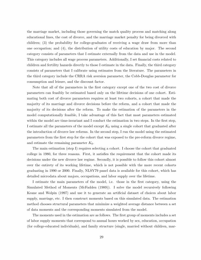
the marriage market, including those governing the match quality process and matching along

educational lines, the cost of divorce, and the marriage market penalty for being divorced with

children; (3) the probability for college-graduates of receiving a wage draw from more than

one occupation; and (4), the distribution of utility costs of education by major. The second

category consists of parameters that I estimate externally from the data and use in the model.

This category includes all wage process parameters. Additionally, I set financial costs related to

children and fertility hazards directly to those I estimate in the data. Finally, the third category

consists of parameters that I calibrate using estimates from the literature. The parameters in

the third category include the CRRA risk aversion parameter, the Cobb-Douglas parameter for

consumption and leisure, and the discount factor.

Note that all of the parameters in the first category except one of the two cost of divorce

parameters can feasibly be estimated based only on the lifetime decisions of one cohort. Esti-

mating both cost of divorce parameters requires at least two cohorts, a cohort that made the

majority of its marriage and divorce decisions before the reform, and a cohort that made the

majority of its decisions after the reform. To make the estimation of the parameters in the

model computationally feasible, I take advantage of this fact that most parameters estimated

within the model are time-invariant and I conduct the estimation in two steps. In the first step,

I estimate all the parameters of the model except K0 using a single cohort that graduated after

the introduction of divorce law reforms. In the second step, I run the model using the estimated

parameters from the first step for the cohort that was exposed to the pre-reform divorce regime,

and estimate the remaining parameter K0.

The main estimation (step I) requires selecting a cohort. I choose the cohort that graduated

college in 1980, for three reasons. First, it satisfies the requirement that the cohort made its

decisions under the new divorce law regime. Secondly, it is possible to follow this cohort almost

over the entirety of its working lifetime, which is not possible with the more recent cohorts

graduating in 1990 or 2000. Finally, NLSY79 panel data is available for this cohort, which has

detailed microdata about majors, occupations, and labor supply over the lifetime.

I estimate the main parameters of the model, i.e. those in the first category, using the

Simulated Method of Moments (McFadden (1989)). I solve the model recursively following

Keane and Wolpin (1997) and use it to generate an artificial dataset of choices about labor

supply, marriage, etc. I then construct moments based on this simulated data. The estimation

method chooses structural parameters that minimize a weighted average distance between a set

of data moments and the corresponding moments simulated from the model.

The moments used in the estimation are as follows. The first group of moments includes a set

of labor supply moments that correspond to annual hours worked by sex, education, occupation

(for college-educated individuals), and family structure (single, married without children, mar-

29

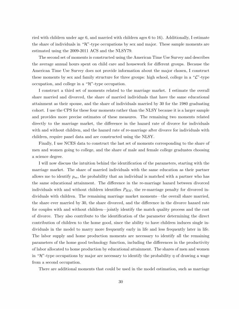
ried with children under age 6, and married with children ages 6 to 16). Additionally, I estimate

the share of individuals in “H”-type occupations by sex and major. These sample moments are

estimated using the 2009-2011 ACS and the NLSY79.

The second set of moments is constructed using the American Time Use Survey and describes

the average annual hours spent on child care and housework for different groups. Because the

American Time Use Survey does not provide information about the major chosen, I construct

these moments by sex and family structure for three groups: high school, college in a “L”-type

occupation, and college in a “H”-type occupation.

I construct a third set of moments related to the marriage market. I estimate the overall

share married and divorced, the share of married individuals that have the same educational

attainment as their spouse, and the share of individuals married by 30 for the 1980 graduating

cohort. I use the CPS for these four moments rather than the NLSY because it is a larger sample

and provides more precise estimates of these measures. The remaining two moments related

directly to the marriage market, the difference in the hazard rate of divorce for individuals

with and without children, and the hazard rate of re-marriage after divorce for individuals with

children, require panel data and are constructed using the NLSY.

Finally, I use NCES data to construct the last set of moments corresponding to the share of

men and women going to college, and the share of male and female college graduates choosing

a science degree.

I will now discuss the intuition behind the identification of the parameters, starting with the

marriage market. The share of married individuals with the same education as their partner

allows me to identify pm, the probability that an individual is matched with a partner who has

the same educational attainment. The difference in the re-marriage hazard between divorced

individuals with and without children identifies PRM , the re-marriage penalty for divorced in-

dividuals with children. The remaining marriage market moments—the overall share married,

the share ever married by 30, the share divorced, and the difference in the divorce hazard rate

for couples with and without children—jointly identify the match quality process and the cost

of divorce. They also contribute to the identification of the parameter determining the direct

contribution of children to the home good, since the ability to have children induces single in-

dividuals in the model to marry more frequently early in life and less frequently later in life.

The labor supply and home production moments are necessary to identify all the remaining

parameters of the home good technology function, including the differences in the productivity

of labor allocated to home production by educational attainment. The shares of men and women

in “H”-type occupations by major are necessary to identify the probability η of drawing a wage

from a second occupation.

There are additional moments that could be used in the model estimation, such as marriage

30

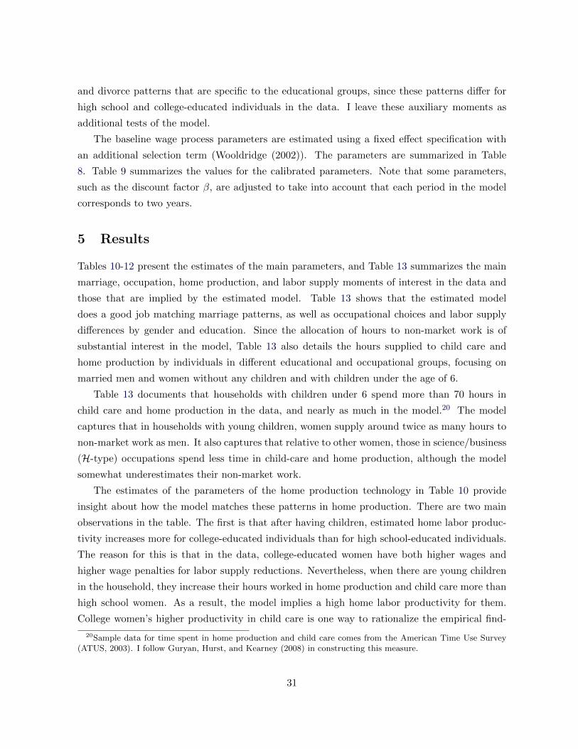
and divorce patterns that are specific to the educational groups, since these patterns differ for

high school and college-educated individuals in the data. I leave these auxiliary moments as

additional tests of the model.

The baseline wage process parameters are estimated using a fixed effect specification with

an additional selection term (Wooldridge (2002)). The parameters are summarized in Table

8. Table 9 summarizes the values for the calibrated parameters. Note that some parameters,

such as the discount factor β, are adjusted to take into account that each period in the model

corresponds to two years.

5 Results

Tables 10-12 present the estimates of the main parameters, and Table 13 summarizes the main

marriage, occupation, home production, and labor supply moments of interest in the data and

those that are implied by the estimated model. Table 13 shows that the estimated model

does a good job matching marriage patterns, as well as occupational choices and labor supply

differences by gender and education. Since the allocation of hours to non-market work is of

substantial interest in the model, Table 13 also details the hours supplied to child care and

home production by individuals in different educational and occupational groups, focusing on

married men and women without any children and with children under the age of 6.

Table 13 documents that households with children under 6 spend more than 70 hours in

child care and home production in the data, and nearly as much in the model.20 The model

captures that in households with young children, women supply around twice as many hours to

non-market work as men. It also captures that relative to other women, those in science/business

(H-type) occupations spend less time in child-care and home production, although the model

somewhat underestimates their non-market work.

The estimates of the parameters of the home production technology in Table 10 provide

insight about how the model matches these patterns in home production. There are two main

observations in the table. The first is that after having children, estimated home labor produc-

tivity increases more for college-educated individuals than for high school-educated individuals.

The reason for this is that in the data, college-educated women have both higher wages and

higher wage penalties for labor supply reductions. Nevertheless, when there are young children

in the household, they increase their hours worked in home production and child care more than

high school women. As a result, the model implies a high home labor productivity for them.

College women’s higher productivity in child care is one way to rationalize the empirical find-

20Sample data for time spent in home production and child care comes from the American Time Use Survey(ATUS, 2003). I follow Guryan, Hurst, and Kearney (2008) in constructing this measure.

31

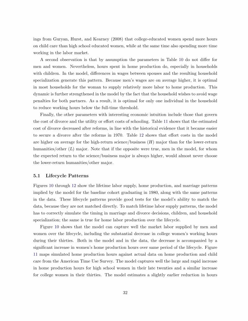
ings from Guryan, Hurst, and Kearney (2008) that college-educated women spend more hours

on child care than high school educated women, while at the same time also spending more time

working in the labor market.

A second observation is that by assumption the parameters in Table 10 do not differ for

men and women. Nevertheless, hours spent in home production do, especially in households

with children. In the model, differences in wages between spouses and the resulting household

specialization generate this pattern. Because men’s wages are on average higher, it is optimal

in most households for the woman to supply relatively more labor to home production. This

dynamic is further strengthened in the model by the fact that the household wishes to avoid wage

penalties for both partners. As a result, it is optimal for only one individual in the household

to reduce working hours below the full-time threshold.

Finally, the other parameters with interesting economic intuition include those that govern

the cost of divorce and the utility or effort costs of schooling. Table 11 shows that the estimated

cost of divorce decreased after reforms, in line with the historical evidence that it became easier

to secure a divorce after the reforms in 1970. Table 12 shows that effort costs in the model

are higher on average for the high-return science/business (H) major than for the lower-return

humanities/other (L) major. Note that if the opposite were true, men in the model, for whom

the expected return to the science/business major is always higher, would almost never choose

the lower-return humanities/other major.

5.1 Lifecycle Patterns

Figures 10 through 12 show the lifetime labor supply, home production, and marriage patterns

implied by the model for the baseline cohort graduating in 1980, along with the same patterns

in the data. These lifecycle patterns provide good tests for the model’s ability to match the

data, because they are not matched directly. To match lifetime labor supply patterns, the model

has to correctly simulate the timing in marriage and divorce decisions, children, and household

specialization; the same is true for home labor production over the lifecycle.

Figure 10 shows that the model can capture well the market labor supplied by men and

women over the lifecycle, including the substantial decrease in college women’s working hours

during their thirties. Both in the model and in the data, the decrease is accompanied by a

significant increase in women’s home production hours over same period of the lifecycle. Figure

11 maps simulated home production hours against actual data on home production and child

care from the American Time Use Survey. The model captures well the large and rapid increase

in home production hours for high school women in their late twenties and a similar increase

for college women in their thirties. The model estimates a slightly earlier reduction in hours

32

worked in home production relative to the data. It also overestimates somewhat labor supply

to the market at the end of the lifecycle for both men and women. Otherwise, it captures well

the lifecycle dynamics in time allocated to market and to home production, as well as difference

in these patterns across sex and educational groups.

Figure 12 graphs lifecycle marriage and divorce patterns. In the estimation, I do not con-

struct separate marriage and divorce moments for high school and college-educated individuals.

Matching these differences across educational groups therefore constitutes an additional test

for the model. Figure 12 shows that the model captures that high school educated individuals

marry earlier, although this result is mechanical, since individuals who choose to go to college

in the model enter the marriage market only after they complete their education. However, the

differences in divorce patterns provide a validity test for the model, and the model correctly

predicts the higher share divorced among high school-educated individuals. The reason for this

is that college-educated couples in the model have higher marital surplus, both because they

have higher productivity of home labor, and also because they allocate more resources to the

market good component of the public home good.

Finally, Figure 13 and Table 14 focus on occupational choices and choices of major for

men and women. Figure 13 shows that the model captures well that women enter into sci-

ence/business (H-type) occupations at a significantly lower rate than men, regardless of major.

This lifecycle pattern is driven partly by the fact that both in the model and in the data many

women do not enter into the low-flexibility science/business occupation in the first place, even

if they have the science/business major.

Table 14 shows how these patterns in labor supply and occupational choices generate the

expected returns to different majors for women and men. The table records the share of indi-

viduals choosing each major in the 1980 cohort and, for expositional purposes, also the model’s

implied expected return in terms of discounted lifetime utility for each major for women and for

men. The purpose of showing the latter is to provide intuition for how the model generates the

different shares of men and women going to college and choosing different majors, since indi-

viduals make their educational choices partly based on these expected overall returns in lifetime

utility, and partly based on their own effort costs for each major.

Table 14 records the expected utility returns in two steps. First, it records the implied

return to the humanities/other (L) major relative to going to high school. This return is higher

for women. Next, it records the additional return to a science/business (H) major relative to

a humanities/other (L) major. This return is substantially higher for men than for women,

although it is positive for both sexes.

The reason that the model implies a high expected return to the humanities/other major

for women is that even though the premium for this type of major is relatively low, it increases

33

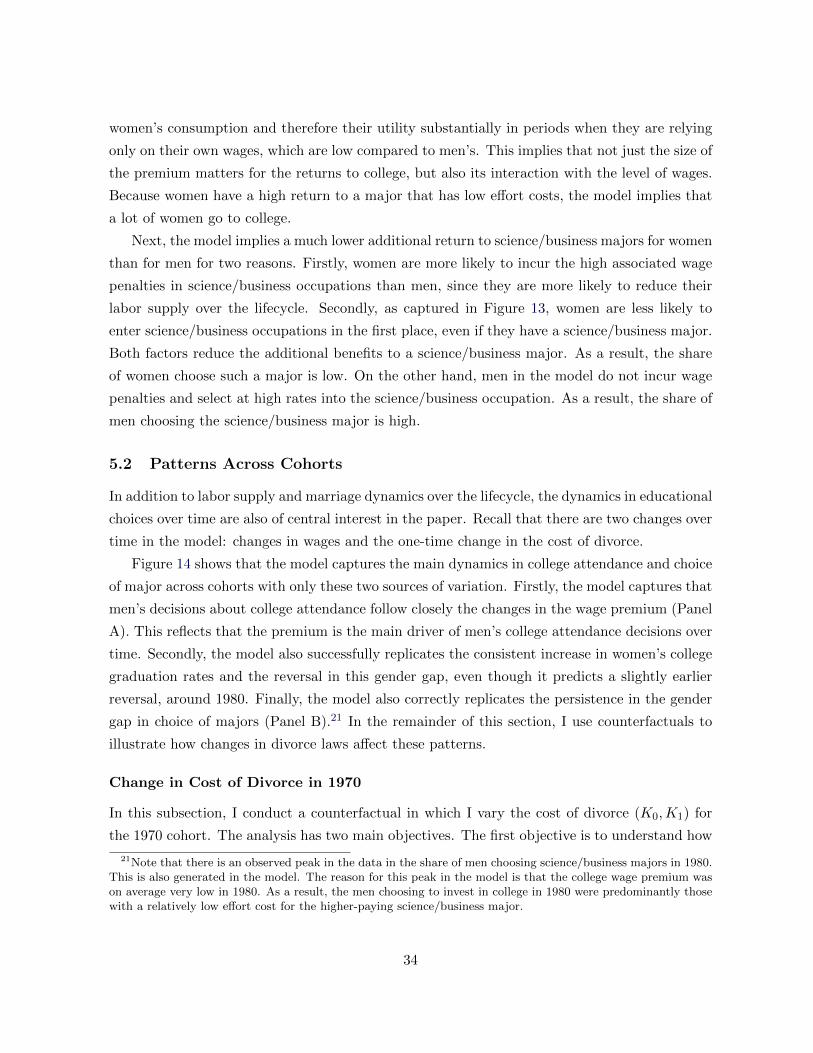
women’s consumption and therefore their utility substantially in periods when they are relying

only on their own wages, which are low compared to men’s. This implies that not just the size of

the premium matters for the returns to college, but also its interaction with the level of wages.

Because women have a high return to a major that has low effort costs, the model implies that

a lot of women go to college.

Next, the model implies a much lower additional return to science/business majors for women

than for men for two reasons. Firstly, women are more likely to incur the high associated wage

penalties in science/business occupations than men, since they are more likely to reduce their

labor supply over the lifecycle. Secondly, as captured in Figure 13, women are less likely to

enter science/business occupations in the first place, even if they have a science/business major.

Both factors reduce the additional benefits to a science/business major. As a result, the share

of women choose such a major is low. On the other hand, men in the model do not incur wage

penalties and select at high rates into the science/business occupation. As a result, the share of

men choosing the science/business major is high.

5.2 Patterns Across Cohorts

In addition to labor supply and marriage dynamics over the lifecycle, the dynamics in educational

choices over time are also of central interest in the paper. Recall that there are two changes over

time in the model: changes in wages and the one-time change in the cost of divorce.

Figure 14 shows that the model captures the main dynamics in college attendance and choice

of major across cohorts with only these two sources of variation. Firstly, the model captures that

men’s decisions about college attendance follow closely the changes in the wage premium (Panel

A). This reflects that the premium is the main driver of men’s college attendance decisions over

time. Secondly, the model also successfully replicates the consistent increase in women’s college

graduation rates and the reversal in this gender gap, even though it predicts a slightly earlier

reversal, around 1980. Finally, the model also correctly replicates the persistence in the gender

gap in choice of majors (Panel B).21 In the remainder of this section, I use counterfactuals to

illustrate how changes in divorce laws affect these patterns.

Change in Cost of Divorce in 1970

In this subsection, I conduct a counterfactual in which I vary the cost of divorce (K0,K1) for

the 1970 cohort. The analysis has two main objectives. The first objective is to understand how

21Note that there is an observed peak in the data in the share of men choosing science/business majors in 1980.This is also generated in the model. The reason for this peak in the model is that the college wage premium wason average very low in 1980. As a result, the men choosing to invest in college in 1980 were predominantly thosewith a relatively low effort cost for the higher-paying science/business major.

34

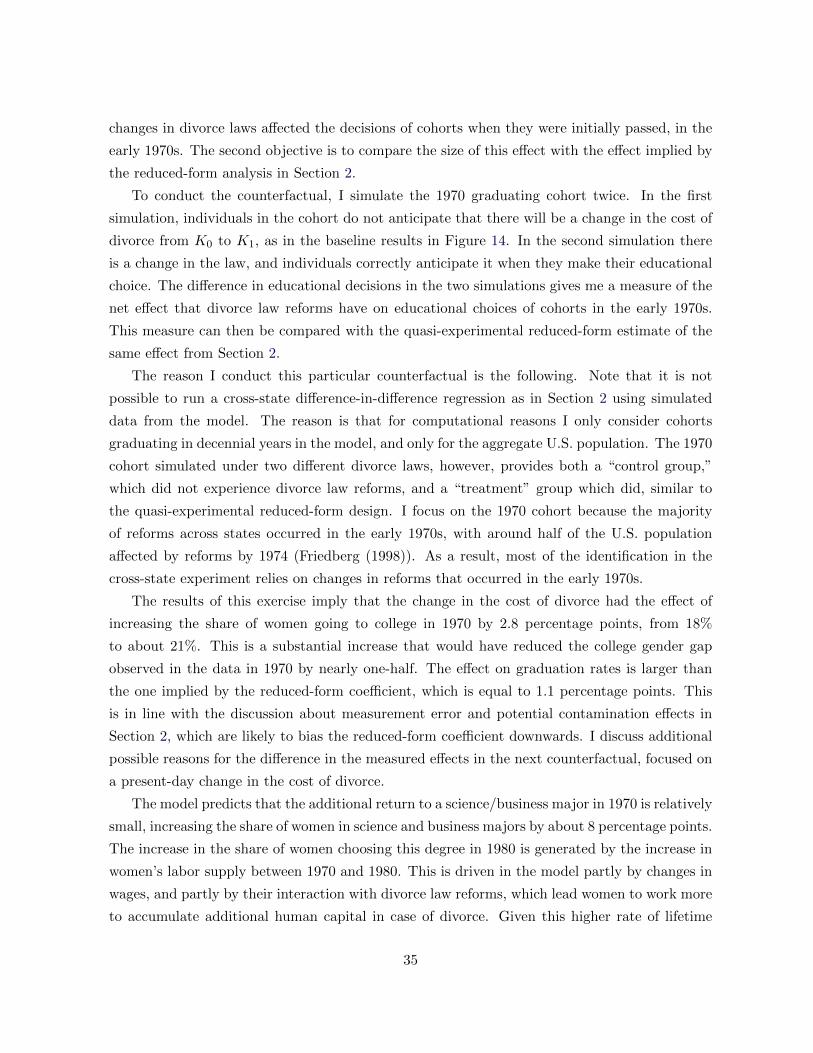
changes in divorce laws affected the decisions of cohorts when they were initially passed, in the

early 1970s. The second objective is to compare the size of this effect with the effect implied by

the reduced-form analysis in Section 2.

To conduct the counterfactual, I simulate the 1970 graduating cohort twice. In the first

simulation, individuals in the cohort do not anticipate that there will be a change in the cost of

divorce from K0 to K1, as in the baseline results in Figure 14. In the second simulation there

is a change in the law, and individuals correctly anticipate it when they make their educational

choice. The difference in educational decisions in the two simulations gives me a measure of the

net effect that divorce law reforms have on educational choices of cohorts in the early 1970s.

This measure can then be compared with the quasi-experimental reduced-form estimate of the

same effect from Section 2.

The reason I conduct this particular counterfactual is the following. Note that it is not

possible to run a cross-state difference-in-difference regression as in Section 2 using simulated

data from the model. The reason is that for computational reasons I only consider cohorts

graduating in decennial years in the model, and only for the aggregate U.S. population. The 1970

cohort simulated under two different divorce laws, however, provides both a “control group,”

which did not experience divorce law reforms, and a “treatment” group which did, similar to

the quasi-experimental reduced-form design. I focus on the 1970 cohort because the majority

of reforms across states occurred in the early 1970s, with around half of the U.S. population

affected by reforms by 1974 (Friedberg (1998)). As a result, most of the identification in the

cross-state experiment relies on changes in reforms that occurred in the early 1970s.

The results of this exercise imply that the change in the cost of divorce had the effect of

increasing the share of women going to college in 1970 by 2.8 percentage points, from 18%

to about 21%. This is a substantial increase that would have reduced the college gender gap

observed in the data in 1970 by nearly one-half. The effect on graduation rates is larger than

the one implied by the reduced-form coefficient, which is equal to 1.1 percentage points. This

is in line with the discussion about measurement error and potential contamination effects in

Section 2, which are likely to bias the reduced-form coefficient downwards. I discuss additional

possible reasons for the difference in the measured effects in the next counterfactual, focused on

a present-day change in the cost of divorce.

The model predicts that the additional return to a science/business major in 1970 is relatively

small, increasing the share of women in science and business majors by about 8 percentage points.

The increase in the share of women choosing this degree in 1980 is generated by the increase in

women’s labor supply between 1970 and 1980. This is driven in the model partly by changes in

wages, and partly by their interaction with divorce law reforms, which lead women to work more

to accumulate additional human capital in case of divorce. Given this higher rate of lifetime

35

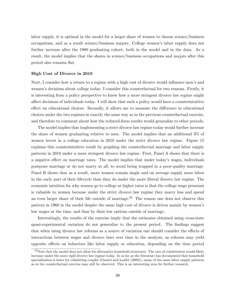
labor supply, it is optimal in the model for a larger share of women to choose science/business

occupations, and as a result science/business majors. College women’s labor supply does not

further increase after the 1980 graduating cohort, both in the model and in the data. As a

result, the model implies that the shares in science/business occupations and majors after this

period also remains flat.

High Cost of Divorce in 2010

Next, I consider how a return to a regime with a high cost of divorce would influence men’s and

women’s decisions about college today. I consider this counterfactual for two reasons. Firstly, it

is interesting from a policy perspective to know how a more stringent divorce law regime might

affect decisions of individuals today. I will show that such a policy would have a counterintuitive

effect on educational choices. Secondly, it allows me to measure the difference in educational

choices under the two regimes in exactly the same way as in the previous counterfactual exercise,

and therefore to comment about how the reduced-form results would generalize to other periods.

The model implies that implementing a strict divorce law regime today would further increase

the share of women graduating relative to men. The model implies that an additional 3% of

women invest in a college education in 2010 under the strict divorce law regime. Figure 15

explains this counterintuitive result by graphing the counterfactual marriage and labor supply

patterns in 2010 under a more stringent divorce law regime. First, Panel A shows that there is

a negative effect on marriage rates. The model implies that under today’s wages, individuals

postpone marriage or do not marry at all, to avoid being trapped in a poor-quality marriage.

Panel B shows that as a result, more women remain single and on average supply more labor

in the early part of their lifecycle than they do under the more liberal divorce law regime. The

economic intuition for why women go to college at higher rates is that the college wage premium

is valuable to women because under the strict divorce law regime they marry less and spend

an even larger share of their life outside of marriage.22 The reason one does not observe this

pattern in 1960 in the model despite the same high cost of divorce is driven mainly by women’s

low wages at the time, and thus by their low options outside of marriage.

Interestingly, the results of the exercise imply that the estimates obtained using cross-state

quasi-experimental variation do not generalize to the present period. The findings suggest

that when using divorce law reforms as a source of variation one should consider the effects of

interactions between wages and divorce laws over time in the analysis, as reforms may yield

opposite effects on behaviors like labor supply or education, depending on the time period

22Note that the model does not allow for alternative household structures. The rate of cohabitation would likelyincrease under the more rigid divorce law regime today. In as far as the literature has documented that householdspecialization is lower for cohabiting couples (Gemici and Laufer (2009)), many of the same labor supply patternsas in the counterfactual exercise may still be observed. This is an interesting area for further research.

36

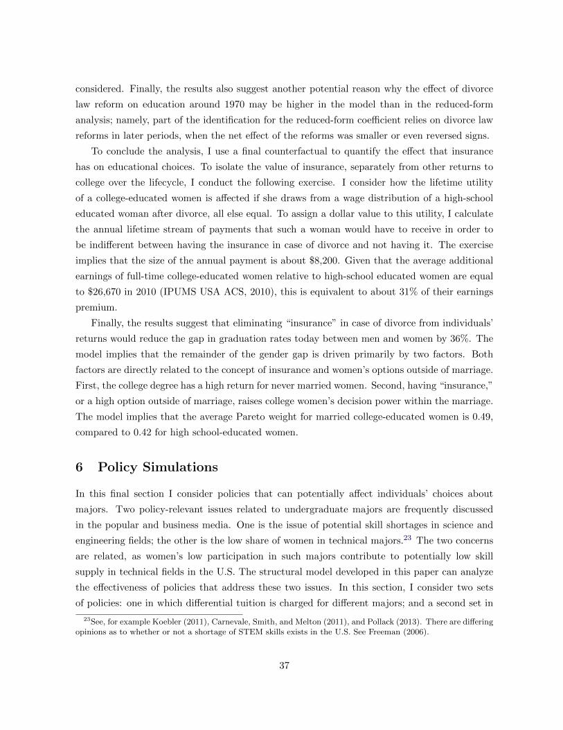
considered. Finally, the results also suggest another potential reason why the effect of divorce

law reform on education around 1970 may be higher in the model than in the reduced-form

analysis; namely, part of the identification for the reduced-form coefficient relies on divorce law

reforms in later periods, when the net effect of the reforms was smaller or even reversed signs.

To conclude the analysis, I use a final counterfactual to quantify the effect that insurance

has on educational choices. To isolate the value of insurance, separately from other returns to

college over the lifecycle, I conduct the following exercise. I consider how the lifetime utility

of a college-educated women is affected if she draws from a wage distribution of a high-school

educated woman after divorce, all else equal. To assign a dollar value to this utility, I calculate

the annual lifetime stream of payments that such a woman would have to receive in order to

be indifferent between having the insurance in case of divorce and not having it. The exercise

implies that the size of the annual payment is about $8,200. Given that the average additional

earnings of full-time college-educated women relative to high-school educated women are equal

to $26,670 in 2010 (IPUMS USA ACS, 2010), this is equivalent to about 31% of their earnings

premium.

Finally, the results suggest that eliminating “insurance” in case of divorce from individuals’

returns would reduce the gap in graduation rates today between men and women by 36%. The

model implies that the remainder of the gender gap is driven primarily by two factors. Both

factors are directly related to the concept of insurance and women’s options outside of marriage.

First, the college degree has a high return for never married women. Second, having “insurance,”

or a high option outside of marriage, raises college women’s decision power within the marriage.

The model implies that the average Pareto weight for married college-educated women is 0.49,

compared to 0.42 for high school-educated women.

6 Policy Simulations

In this final section I consider policies that can potentially affect individuals’ choices about

majors. Two policy-relevant issues related to undergraduate majors are frequently discussed

in the popular and business media. One is the issue of potential skill shortages in science and

engineering fields; the other is the low share of women in technical majors.23 The two concerns

are related, as women’s low participation in such majors contribute to potentially low skill

supply in technical fields in the U.S. The structural model developed in this paper can analyze

the effectiveness of policies that address these two issues. In this section, I consider two sets

of policies: one in which differential tuition is charged for different majors; and a second set in

23See, for example Koebler (2011), Carnevale, Smith, and Melton (2011), and Pollack (2013). There are differingopinions as to whether or not a shortage of STEM skills exists in the U.S. See Freeman (2006).

37

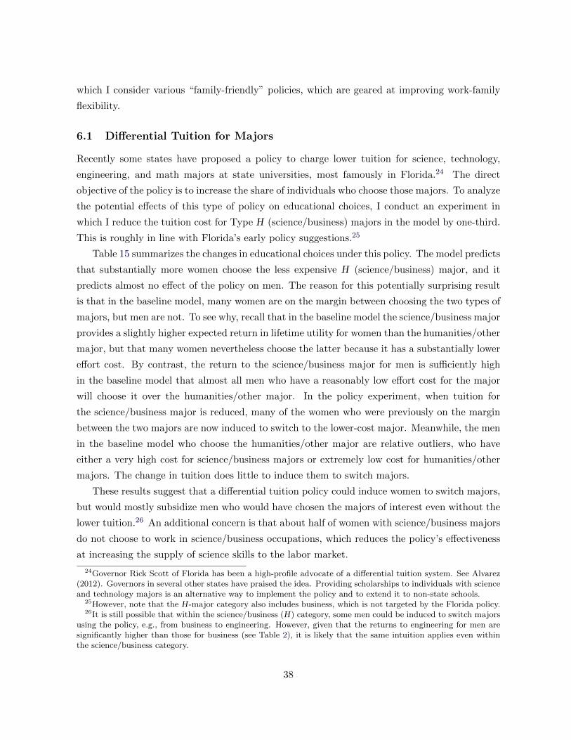
which I consider various “family-friendly” policies, which are geared at improving work-family

flexibility.

6.1 Differential Tuition for Majors

Recently some states have proposed a policy to charge lower tuition for science, technology,

engineering, and math majors at state universities, most famously in Florida.24 The direct

objective of the policy is to increase the share of individuals who choose those majors. To analyze

the potential effects of this type of policy on educational choices, I conduct an experiment in

which I reduce the tuition cost for Type H (science/business) majors in the model by one-third.

This is roughly in line with Florida’s early policy suggestions.25

Table 15 summarizes the changes in educational choices under this policy. The model predicts

that substantially more women choose the less expensive H (science/business) major, and it

predicts almost no effect of the policy on men. The reason for this potentially surprising result

is that in the baseline model, many women are on the margin between choosing the two types of

majors, but men are not. To see why, recall that in the baseline model the science/business major

provides a slightly higher expected return in lifetime utility for women than the humanities/other

major, but that many women nevertheless choose the latter because it has a substantially lower

effort cost. By contrast, the return to the science/business major for men is sufficiently high

in the baseline model that almost all men who have a reasonably low effort cost for the major

will choose it over the humanities/other major. In the policy experiment, when tuition for

the science/business major is reduced, many of the women who were previously on the margin

between the two majors are now induced to switch to the lower-cost major. Meanwhile, the men

in the baseline model who choose the humanities/other major are relative outliers, who have

either a very high cost for science/business majors or extremely low cost for humanities/other

majors. The change in tuition does little to induce them to switch majors.

These results suggest that a differential tuition policy could induce women to switch majors,

but would mostly subsidize men who would have chosen the majors of interest even without the

lower tuition.26 An additional concern is that about half of women with science/business majors

do not choose to work in science/business occupations, which reduces the policy’s effectiveness

at increasing the supply of science skills to the labor market.

24Governor Rick Scott of Florida has been a high-profile advocate of a differential tuition system. See Alvarez(2012). Governors in several other states have praised the idea. Providing scholarships to individuals with scienceand technology majors is an alternative way to implement the policy and to extend it to non-state schools.

25However, note that the H -major category also includes business, which is not targeted by the Florida policy.26It is still possible that within the science/business (H) category, some men could be induced to switch majors

using the policy, e.g., from business to engineering. However, given that the returns to engineering for men aresignificantly higher than those for business (see Table 2), it is likely that the same intuition applies even withinthe science/business category.

38

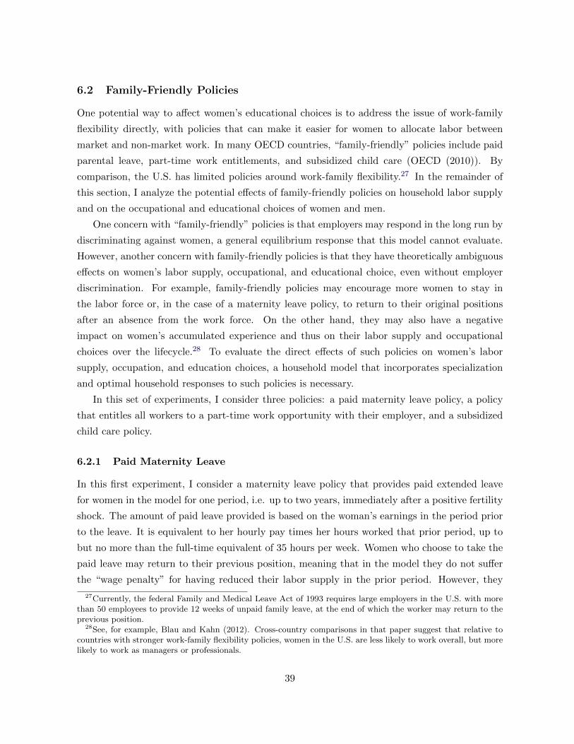
6.2 Family-Friendly Policies

One potential way to affect women’s educational choices is to address the issue of work-family

flexibility directly, with policies that can make it easier for women to allocate labor between

market and non-market work. In many OECD countries, “family-friendly” policies include paid

parental leave, part-time work entitlements, and subsidized child care (OECD (2010)). By

comparison, the U.S. has limited policies around work-family flexibility.27 In the remainder of

this section, I analyze the potential effects of family-friendly policies on household labor supply

and on the occupational and educational choices of women and men.

One concern with “family-friendly” policies is that employers may respond in the long run by

discriminating against women, a general equilibrium response that this model cannot evaluate.

However, another concern with family-friendly policies is that they have theoretically ambiguous

effects on women’s labor supply, occupational, and educational choice, even without employer

discrimination. For example, family-friendly policies may encourage more women to stay in

the labor force or, in the case of a maternity leave policy, to return to their original positions

after an absence from the work force. On the other hand, they may also have a negative

impact on women’s accumulated experience and thus on their labor supply and occupational

choices over the lifecycle.28 To evaluate the direct effects of such policies on women’s labor

supply, occupation, and education choices, a household model that incorporates specialization

and optimal household responses to such policies is necessary.

In this set of experiments, I consider three policies: a paid maternity leave policy, a policy

that entitles all workers to a part-time work opportunity with their employer, and a subsidized

child care policy.

6.2.1 Paid Maternity Leave

In this first experiment, I consider a maternity leave policy that provides paid extended leave

for women in the model for one period, i.e. up to two years, immediately after a positive fertility

shock. The amount of paid leave provided is based on the woman’s earnings in the period prior

to the leave. It is equivalent to her hourly pay times her hours worked that prior period, up to

but no more than the full-time equivalent of 35 hours per week. Women who choose to take the

paid leave may return to their previous position, meaning that in the model they do not suffer

the “wage penalty” for having reduced their labor supply in the prior period. However, they

27Currently, the federal Family and Medical Leave Act of 1993 requires large employers in the U.S. with morethan 50 employees to provide 12 weeks of unpaid family leave, at the end of which the worker may return to theprevious position.

28See, for example, Blau and Kahn (2012). Cross-country comparisons in that paper suggest that relative tocountries with stronger work-family flexibility policies, women in the U.S. are less likely to work overall, but morelikely to work as managers or professionals.

39

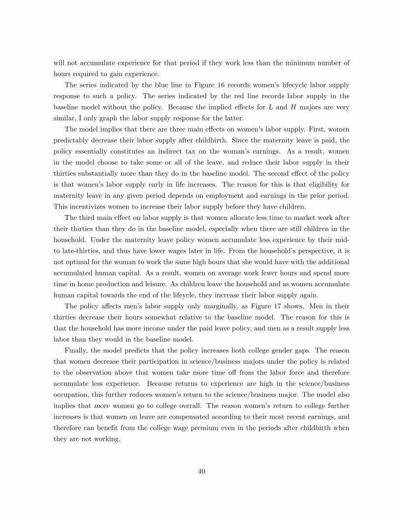
will not accumulate experience for that period if they work less than the minimum number of

hours required to gain experience.

The series indicated by the blue line in Figure 16 records women’s lifecycle labor supply

response to such a policy. The series indicated by the red line records labor supply in the

baseline model without the policy. Because the implied effects for L and H majors are very

similar, I only graph the labor supply response for the latter.

The model implies that there are three main effects on women’s labor supply. First, women

predictably decrease their labor supply after childbirth. Since the maternity leave is paid, the

policy essentially constitutes an indirect tax on the woman’s earnings. As a result, women

in the model choose to take some or all of the leave, and reduce their labor supply in their

thirties substantially more than they do in the baseline model. The second effect of the policy

is that women’s labor supply early in life increases. The reason for this is that eligibility for

maternity leave in any given period depends on employment and earnings in the prior period.

This incentivizes women to increase their labor supply before they have children.

The third main effect on labor supply is that women allocate less time to market work after

their thirties than they do in the baseline model, especially when there are still children in the

household. Under the maternity leave policy women accumulate less experience by their mid-

to late-thirties, and thus have lower wages later in life. From the household’s perspective, it is

not optimal for the woman to work the same high hours that she would have with the additional

accumulated human capital. As a result, women on average work fewer hours and spend more

time in home production and leisure. As children leave the household and as women accumulate

human capital towards the end of the lifeycle, they increase their labor supply again.

The policy affects men’s labor supply only marginally, as Figure 17 shows. Men in their

thirties decrease their hours somewhat relative to the baseline model. The reason for this is

that the household has more income under the paid leave policy, and men as a result supply less

labor than they would in the baseline model.

Finally, the model predicts that the policy increases both college gender gaps. The reason

that women decrease their participation in science/business majors under the policy is related

to the observation above that women take more time off from the labor force and therefore

accumulate less experience. Because returns to experience are high in the science/business

occupation, this further reduces women’s return to the science/business major. The model also

implies that more women go to college overall. The reason women’s return to college further

increases is that women on leave are compensated according to their most recent earnings, and

therefore can benefit from the college wage premium even in the periods after childbirth when

they are not working.

40

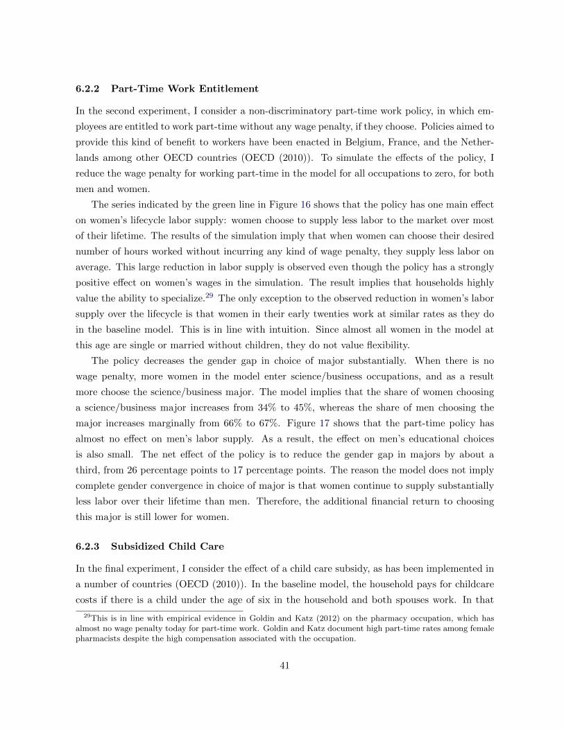
6.2.2 Part-Time Work Entitlement

In the second experiment, I consider a non-discriminatory part-time work policy, in which em-

ployees are entitled to work part-time without any wage penalty, if they choose. Policies aimed to

provide this kind of benefit to workers have been enacted in Belgium, France, and the Nether-

lands among other OECD countries (OECD (2010)). To simulate the effects of the policy, I

reduce the wage penalty for working part-time in the model for all occupations to zero, for both

men and women.

The series indicated by the green line in Figure 16 shows that the policy has one main effect

on women’s lifecycle labor supply: women choose to supply less labor to the market over most

of their lifetime. The results of the simulation imply that when women can choose their desired

number of hours worked without incurring any kind of wage penalty, they supply less labor on

average. This large reduction in labor supply is observed even though the policy has a strongly

positive effect on women’s wages in the simulation. The result implies that households highly

value the ability to specialize.29 The only exception to the observed reduction in women’s labor

supply over the lifecycle is that women in their early twenties work at similar rates as they do

in the baseline model. This is in line with intuition. Since almost all women in the model at

this age are single or married without children, they do not value flexibility.

The policy decreases the gender gap in choice of major substantially. When there is no

wage penalty, more women in the model enter science/business occupations, and as a result

more choose the science/business major. The model implies that the share of women choosing

a science/business major increases from 34% to 45%, whereas the share of men choosing the

major increases marginally from 66% to 67%. Figure 17 shows that the part-time policy has

almost no effect on men’s labor supply. As a result, the effect on men’s educational choices

is also small. The net effect of the policy is to reduce the gender gap in majors by about a

third, from 26 percentage points to 17 percentage points. The reason the model does not imply

complete gender convergence in choice of major is that women continue to supply substantially

less labor over their lifetime than men. Therefore, the additional financial return to choosing

this major is still lower for women.

6.2.3 Subsidized Child Care

In the final experiment, I consider the effect of a child care subsidy, as has been implemented in

a number of countries (OECD (2010)). In the baseline model, the household pays for childcare

costs if there is a child under the age of six in the household and both spouses work. In that

29This is in line with empirical evidence in Goldin and Katz (2012) on the pharmacy occupation, which hasalmost no wage penalty today for part-time work. Goldin and Katz document high part-time rates among femalepharmacists despite the high compensation associated with the occupation.

41

case, the household pays an hourly childcare cost for the number of hours worked by the spouse

with the lower labor supply. In this particular policy experiment, I provide a full subsidy, i.e. I

reduce the cost of childcare to zero.30

The series represented by the dotted red line in Figure 16 shows that subsidized child care

has a small effect on women’s labor supply patterns. The policy increases the labor supply of

college women in the model mostly in their early childbearing years. In the baseline model, the

childcare cost is usually an implicit tax on the woman’s wage, since she is typically the one to

provide the lower labor supply in the household. Among college-educated women in the model,

those who respond to the policy are primarily women in science/business occupations with a

low wage draw that period. The effective increase in their wage due to the subsidy is enough

for some of these women to increase labor supply to avoid a wage penalty or to accumulate

experience, which has a high future return. However, because these estimated effects are small,

the implied effects on the returns to education are also minor.

Table 16 summarizes and compares the effects of the three family-friendly policies on educa-

tional choices. As a whole, the policy results suggest that a program that successfully increases

the availability of part-time work would be the most effective in increasing women’s participation

in both science/business occupations and majors.

7 Conclusion

Women today make up the majority of college students in the U.S. and in almost every developed

country around the world (OECD, 2012). At the same time, in all of these countries today women

select systematically into very different majors than men (Vincent-Lancrin (2006)). I document

that in the U.S., there has been almost no convergence between men and women in choices of

major since the mid-1980s, even as women caught up to and rapidly outpaced men in graduation

rates. In 1985, men were about 1.5 times as likely as women to select high-paying science and

business majors, and the same is true today.

I provide evidence that two factors help explain gender differences in college attainment

and choice of major for those in college: first, college degrees provide insurance against very low

income for women, especially in case of divorce; second, majors and their associated occupations

differ substantially in the degree of “work-family flexibility” they offer, such as availability of

part-time work and the size of wage penalties for temporary reductions in labor supply. Both

components of this explanation are related to the gender gap in wages. Because women draw

from a lower wage distribution, they are more likely to seek insurance against very low income

30I set the child care cost to $5.60 per hour, based on data from the Census Bureau on weekly child careexpenditures for mothers of children 5 or under who use child care (Laughlin (2013)).

42

realizations when they are single or divorced, and more likely to specialize at least partly in

non-market work when they are married. Their educational choices reflect this.

To analyze these drivers of educational decisions in greater detail, I construct and estimate

a dynamic structural model of lifecycle marriage, labor supply, occupational and educational

choices. Using the model, I show how changes in marriage patterns following divorce laws

and changes in skill premiums over time affect the educational decisions of different cohorts.

I estimate that the insurance value of a degree for women today is equivalent to about 31%

of their wage premium. I also estimate that the difference in the shares of men and women

choosing science/business majors would decrease by about a third if penalties to labor supply

reductions were equalized across occupations.

More than 75% of college-educated women today have children over the course of their life.31

This means that for the vast majority of college-educated women today the question is not

“children or career,” but rather “children and career, or children and no career.” The findings

in this paper suggest that many college-educated women select lower-paying occupations and

majors to have flexibility to allocate more time to child care and home production, especially

when their children are young. For this reason, I use the structural model to test several policies

that potentially improve work-family flexibility for women across occupations. I find very large

differences in the effects of these policies, with some even further widening both gender gaps

in education. The findings call for more research in the future on flexible policies that make

it easier for women to participate in science and technical occupations, especially as many

developed economies grow increasingly more concerned about the low number of graduates in

science and technical fields.

31In the 2009-2011 ACS, among women with a 4-year college degree, at age forty 75% have a child currently inthe household. This is likely to be a lower bound for the share of college-educated women who ever had a child.

43

References

Alvarez, Lizette. 2012. “Florida May Reduce Tuition for Select Majors.” The New York Times,

December 9.

Bailey, Martha J. 2010. “”Momma’s Got the Pill”: How Anthony Comstock and Griswold

v. Connecticut Shaped US Childbearing.” The American Economic Review 100 (1): pp.

98–129.

Becker, Gary S. 1962. “Investment in Human Capital: A Theoretical Analysis.” Journal of

Political Economy 70 (5): pp. 9–49.

. 1973. “A Theory of Marriage: Part I.” Journal of Political Economy 81 (4): pp.

813–846.

. 1974. “A Theory of Marriage: Part II.” Journal of Political Economy 82 (2): pp.

S11–S26.

Ben-Porath, Yoram. 1967. “The Production of Human Capital and the Life Cycle of Earnings.”

Journal of Political Economy 75 (4): pp. 352–365.

Bernard, Tara Siegel. 2013. “In Paid Family Leave, U.S. Trails Most of the Globe.” The New

York Times, Februrary 22.

Bertrand, Marianne, Claudia Goldin, and Lawrence F. Katz. 2010. “Dynamics of the Gender

Gap for Young Professionals in the Financial and Corporate Sectors.” American Economic

Journal: Applied Economics 2:pp. 228255.

Blau, Francine D., and Lawrence M. Kahn. 2012. “Female Labor Supply: Why is the U.S.

Falling Behind.” IZA Discussion Paper Series, no. 7140.

Carnevale, Anthony P., Nicole Smith, and Michelle Melton. 2011. STEM: Science, Technol-

ogy, Engineering, and Mathematics. Georgetown University Center on Education and the

Workforce.

Charles, Kerwin, and Ming-Ching Luoh. 2003. “Gender Differences in Completed Schooling.”

Review of Economics and Statistics 85 (3): pp. 559–577.

Chiappori, Pierre-Andr, Murat Iyigun, and Yoram Weiss. 2009. “Investment in Schooling and

the Marriage Market.” The American Economic Review 99 (5): pp. 1689–1713.

Duffie, Darrell, and Kenneth J. Singleton. 1993. “Simulated Moments Estimation of Markov

Models of Asset Prices.” Econometrica 61 (4): pp. 929–952.

Fernndez, Raquel, and Joyce Cheng Wong. 2011. “The Disappearing Gender Gap: The Impact

44

of Divorce, Wages, and Preferences on Education Choices and Women’s Work.” NBER

Working Paper, no. 17508.

Freeman, Richard B. 2006. “Labor Market Imbalances: Shortages, Surpluses, or What?”

Federal Reserve Bank of Boston Conference Series.

Friedberg, Leora. 1998. “Did Unilateral Divorce Raise Divorce Rates? Evidence from Panel

Data.” American Economic Review 88 (3): pp. 608–627.

Gemici, Ahu, and Matthew Wiswall. “Evolution of Gender Differences in Post-Secondary Hu-

man Capital Investments: College Majors.” International Economic Review, forthcoming.

Goldin, Claudia, and Lawrence F. Katz. 2011. “The Cost of Workplace Flexibility for High-

Powered Professionals.” The Annals of the American Academy 638 (1): pp. 45–67.

. 2012. “The Most Egalitarian of All Professions: Pharmacy and the Evolution of a

Family-Friendly Occupation.” NBER Working Paper, no. 18410.

Goldin, Claudia, Lawrence F. Katz, and Ilyana Kuziemko. 2006. “The Homecoming of Amer-

ican College Women: The Reversal of the College Gender Gap.” Journal of Economic

Perspectives 20 (4): pp. 133–156.

Gourieroux, Christian, and Alain Monfort. 1996. Simulation-Based Econometric Methods. New

York: Oxford University Press.

Gourieroux, Christian, Alain Monfort, and Eric Renault. 1993. “Indirect Inference.” Journal

of Applied Econometrics 8 (December): S85–118.

Grail, Timothy. 2002. “Custodial Mothers and Fathers and Their Child Support.” U.S. Census

Bureau Current Population Reports.

Gruber, Jonathan. 2004. “Is Making Divorce Easier Bad for Children? The Long-Run Impli-

cations of Unilateral Divorce.” Journal of Labor Economics 22 (4): pp. 799–833.

Guryan, Jonathan, Erik Hurst, and Melissa Kearney. 2008. “Parental Education and Parental

Time with Children.” Journal of Economic Perspectives 22 (3): pp. 23–46.

Herbert, Jacob. 1988. Silent Revolution: The Transformation of Divorce Law in the United

States. Chicago, IL: University of Chicago Press.

Iyigun, Murat, and Randall P. Walsh. 2007. “Building the Family Nest: Premarital Invest-

ments, Marriage Markets, and Spousal Allocations.” The Review of Economic Studies 74

(2): pp. 507–535.

Johnson, William, and Jonathan Skinner. 1986. “Labor Supply and Marital Separation.”

American Economic Review 76 (4): pp. 455–469.

45

Keane, Michael P., and Kenneth Wolpin. 1997. “The Career Decisions of Young Men.” Journal

of Political Economy 105 (3): pp. 473–522.

Killingsworth, Mark R., and James J. Heckman. 1986. “Female Labor Supply: a Survey.”

Handbook of Labor Economics, Edited by O. Ashenfelter and R. Layard, 1:pp. 103–204.

Koebler, Jason. 2011. “Demand, Pay for STEM Skills Skyrocket.” U.S. News and World

Report, October 20.

Lee, Bong-Soo, and Beth Fisher Ingram. 1991. “Simulation Estimation of Time-series Models.”

Journal of Econometrics 47 (2-3): pp. 197–205.

Mazzocco, Maurizio. 2007. “Household Intertemporal Behaviour: A Collective Characterization

and a Test of Commitment.” The Review of Economic Studies 74 (3): pp. 857–895.

Mazzocco, Maurizio, Claudia Ruiz, and Shintaro Yamaguchi. 2009. “Labor Supply, Wealth

Dynamics, and Marriage Decisions.” Manuscript.

McFadden, Daniel. 1989. “A Method of Simulated Moments for Estimation of Discrete Re-

sponse Models Without Numerical Integration.” Econometrica 57 (5): pp. 995–1026.

OECD. 2010. “How Good is Part-Time Work?” OECD Employment Outlook 2010: Moving

beyond the Jobs Crisis.

Pakes, Ariel, and David Pollard. 1989. “Simulation and the Asymptotics of Optimization

Estimators.” Econometrica 57 (5): pp. 1027–1057.

Polachek, Solomon William. 1978. “Sex Differences in College Major.” Industrial and Labor

Relations Review 31 (4): pp. 498508.

. 1981. “Occupational Self-Selection: A Human Capital Approach to Sex Differences in

Occupational Structure.” The Review of Economics and Statistics 63 (1): pp. 60–69.

Pollack, Eileen. 2013. “Why Are There Still So Few Women in Science?” The New York Times,

October 3.

Rampbell, Catherine. 2013. “Coveting Not a Corner Office, but Time at Home.” The New

York Times, July 7.

Stevenson, Betsey, and Justin Wolfers. 2006. “Bargaining in the Shadow of the Law: Divorce

Laws and Family Distress.” Quarterly Journal of Economics 121 (1): pp. 267–288.

Vincent-Lancrin, Stephan. 2006. “The reversal of gender inequalities in higher education:

An on-going trend. Higher Education to 2030.” OECD Volume 1: Demography, pp. pp.

265–298.

46

Voena, Alessandra. 2012. “Yours, Mine and Ours: Do Divorce Laws Affect the Intertemporal

Behavior of Married Couples.” Manuscript.

Wiswall, Matthew, and Basit Zafar. 2013. “Determinants of College Major Choice: Identifica-

tion Using an Information Experiment.” Manuscript.

Wood, Catherine A. 2011. “Employment in Health Care: A Crutch for the Ailing Economy

During the 2007-09 Recession.” Monthly Labor Review 134 (4): pp. 13–18.

47

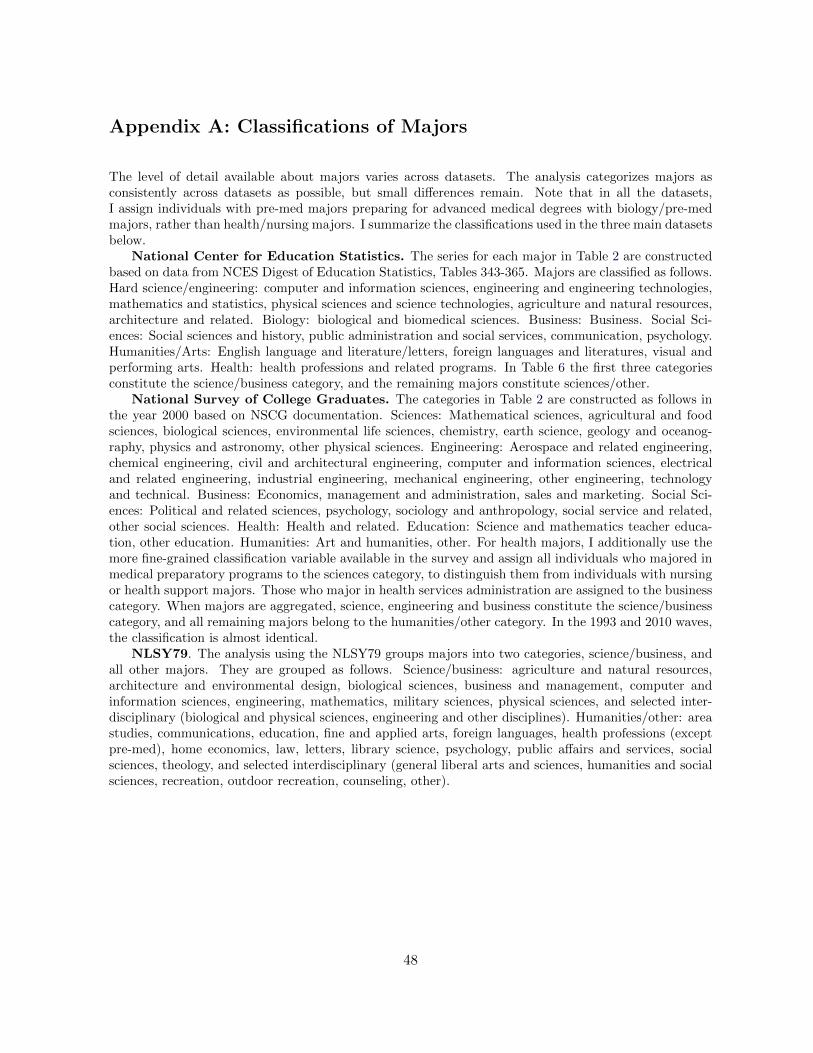
Appendix A: Classifications of Majors

The level of detail available about majors varies across datasets. The analysis categorizes majors asconsistently across datasets as possible, but small differences remain. Note that in all the datasets,I assign individuals with pre-med majors preparing for advanced medical degrees with biology/pre-medmajors, rather than health/nursing majors. I summarize the classifications used in the three main datasetsbelow.

National Center for Education Statistics. The series for each major in Table 2 are constructedbased on data from NCES Digest of Education Statistics, Tables 343-365. Majors are classified as follows.Hard science/engineering: computer and information sciences, engineering and engineering technologies,mathematics and statistics, physical sciences and science technologies, agriculture and natural resources,architecture and related. Biology: biological and biomedical sciences. Business: Business. Social Sci-ences: Social sciences and history, public administration and social services, communication, psychology.Humanities/Arts: English language and literature/letters, foreign languages and literatures, visual andperforming arts. Health: health professions and related programs. In Table 6 the first three categoriesconstitute the science/business category, and the remaining majors constitute sciences/other.

National Survey of College Graduates. The categories in Table 2 are constructed as follows inthe year 2000 based on NSCG documentation. Sciences: Mathematical sciences, agricultural and foodsciences, biological sciences, environmental life sciences, chemistry, earth science, geology and oceanog-raphy, physics and astronomy, other physical sciences. Engineering: Aerospace and related engineering,chemical engineering, civil and architectural engineering, computer and information sciences, electricaland related engineering, industrial engineering, mechanical engineering, other engineering, technologyand technical. Business: Economics, management and administration, sales and marketing. Social Sci-ences: Political and related sciences, psychology, sociology and anthropology, social service and related,other social sciences. Health: Health and related. Education: Science and mathematics teacher educa-tion, other education. Humanities: Art and humanities, other. For health majors, I additionally use themore fine-grained classification variable available in the survey and assign all individuals who majored inmedical preparatory programs to the sciences category, to distinguish them from individuals with nursingor health support majors. Those who major in health services administration are assigned to the businesscategory. When majors are aggregated, science, engineering and business constitute the science/businesscategory, and all remaining majors belong to the humanities/other category. In the 1993 and 2010 waves,the classification is almost identical.

NLSY79. The analysis using the NLSY79 groups majors into two categories, science/business, andall other majors. They are grouped as follows. Science/business: agriculture and natural resources,architecture and environmental design, biological sciences, business and management, computer andinformation sciences, engineering, mathematics, military sciences, physical sciences, and selected inter-disciplinary (biological and physical sciences, engineering and other disciplines). Humanities/other: areastudies, communications, education, fine and applied arts, foreign languages, health professions (exceptpre-med), home economics, law, letters, library science, psychology, public affairs and services, socialsciences, theology, and selected interdisciplinary (general liberal arts and sciences, humanities and socialsciences, recreation, outdoor recreation, counseling, other).

48

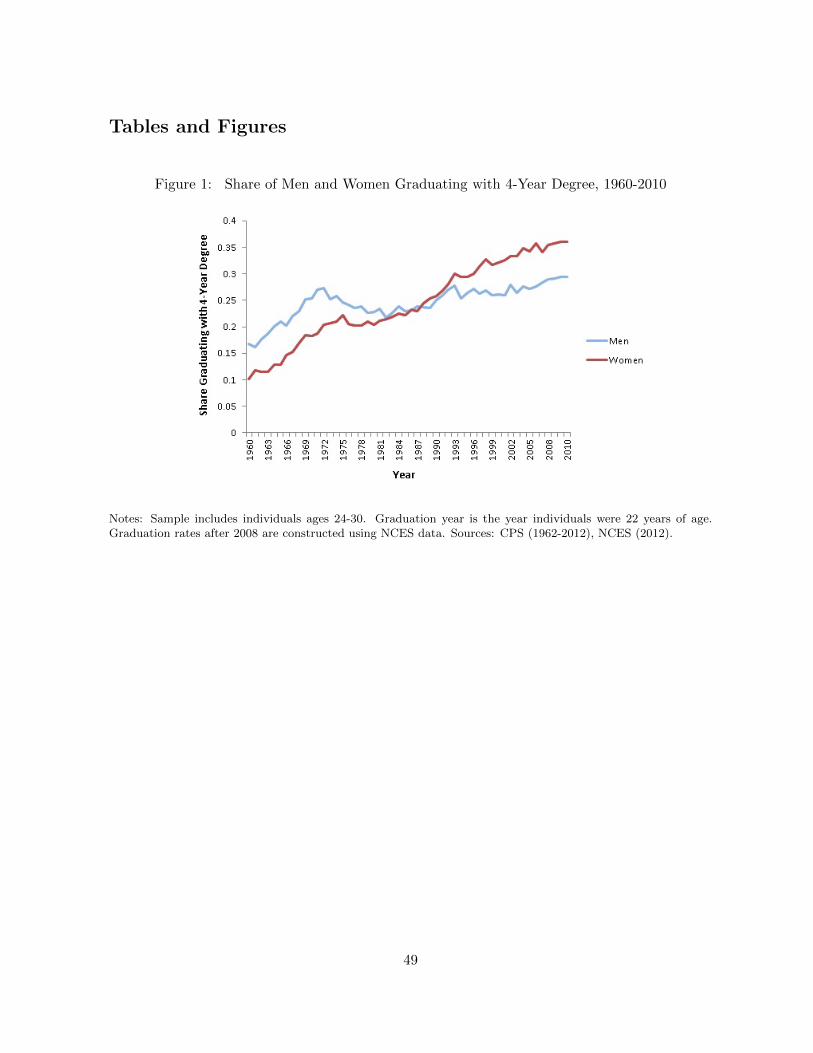
Tables and Figures

Figure 1: Share of Men and Women Graduating with 4-Year Degree, 1960-2010

Notes: Sample includes individuals ages 24-30. Graduation year is the year individuals were 22 years of age.Graduation rates after 2008 are constructed using NCES data. Sources: CPS (1962-2012), NCES (2012).

49

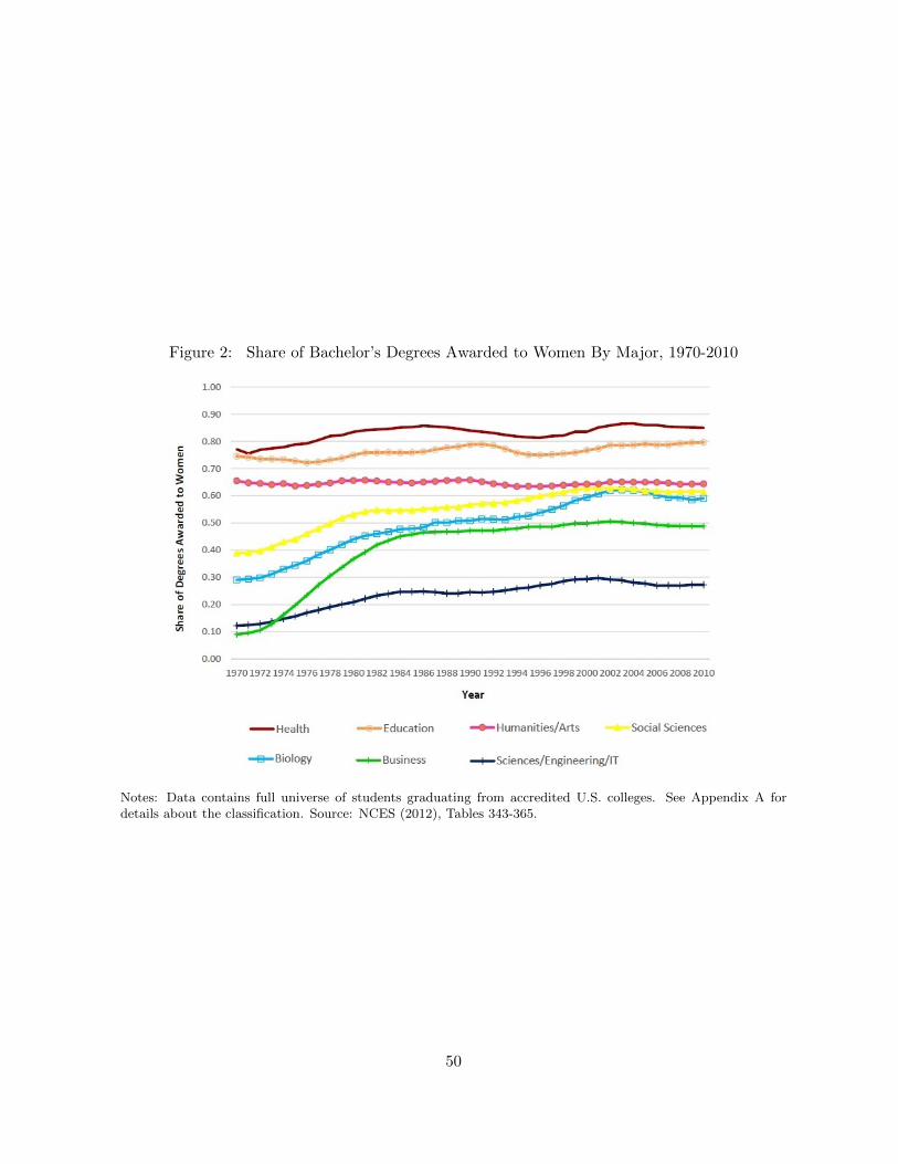
Figure 2: Share of Bachelor’s Degrees Awarded to Women By Major, 1970-2010

Notes: Data contains full universe of students graduating from accredited U.S. colleges. See Appendix A fordetails about the classification. Source: NCES (2012), Tables 343-365.

50

Figure 3: Share Graduating and College Wage Premium, 1960-2012

A. Share Graduating from College B. College Wage Premium

Notes: For Panel A, see notes in Figure 1. In Panel B, the sample includes all individuals ages 25-50, who worked35+ hours in the past week and 48+ weeks in the past year. The wage premium is the difference in log incomebetween college and high school graduates. Source: CPS (1962-2012).

Figure 4: Share Divorced and the Ratio of Women to Men Graduating, by Year

Notes: Share divorced refers to the share of all individuals between 18 and 60 divorced in each calendar year. Thecollege gender gap is the ratio of women to men graduating that calendar year. Source: IPUMS CPS, 1962-2010;NCES, 1960-2010.

51

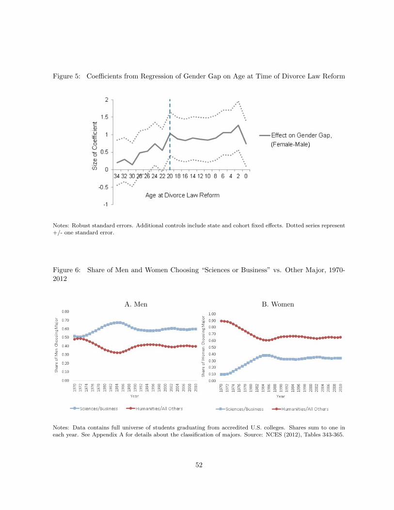
Figure 5: Coefficients from Regression of Gender Gap on Age at Time of Divorce Law Reform

Notes: Robust standard errors. Additional controls include state and cohort fixed effects. Dotted series represent+/- one standard error.

Figure 6: Share of Men and Women Choosing “Sciences or Business” vs. Other Major, 1970-2012

A. Men B. Women

Notes: Data contains full universe of students graduating from accredited U.S. colleges. Shares sum to one ineach year. See Appendix A for details about the classification of majors. Source: NCES (2012), Tables 343-365.

52

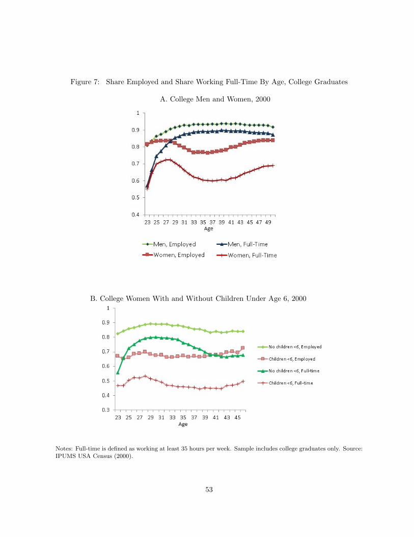
Figure 7: Share Employed and Share Working Full-Time By Age, College Graduates

A. College Men and Women, 2000

B. College Women With and Without Children Under Age 6, 2000

Notes: Full-time is defined as working at least 35 hours per week. Sample includes college graduates only. Source:IPUMS USA Census (2000).

53

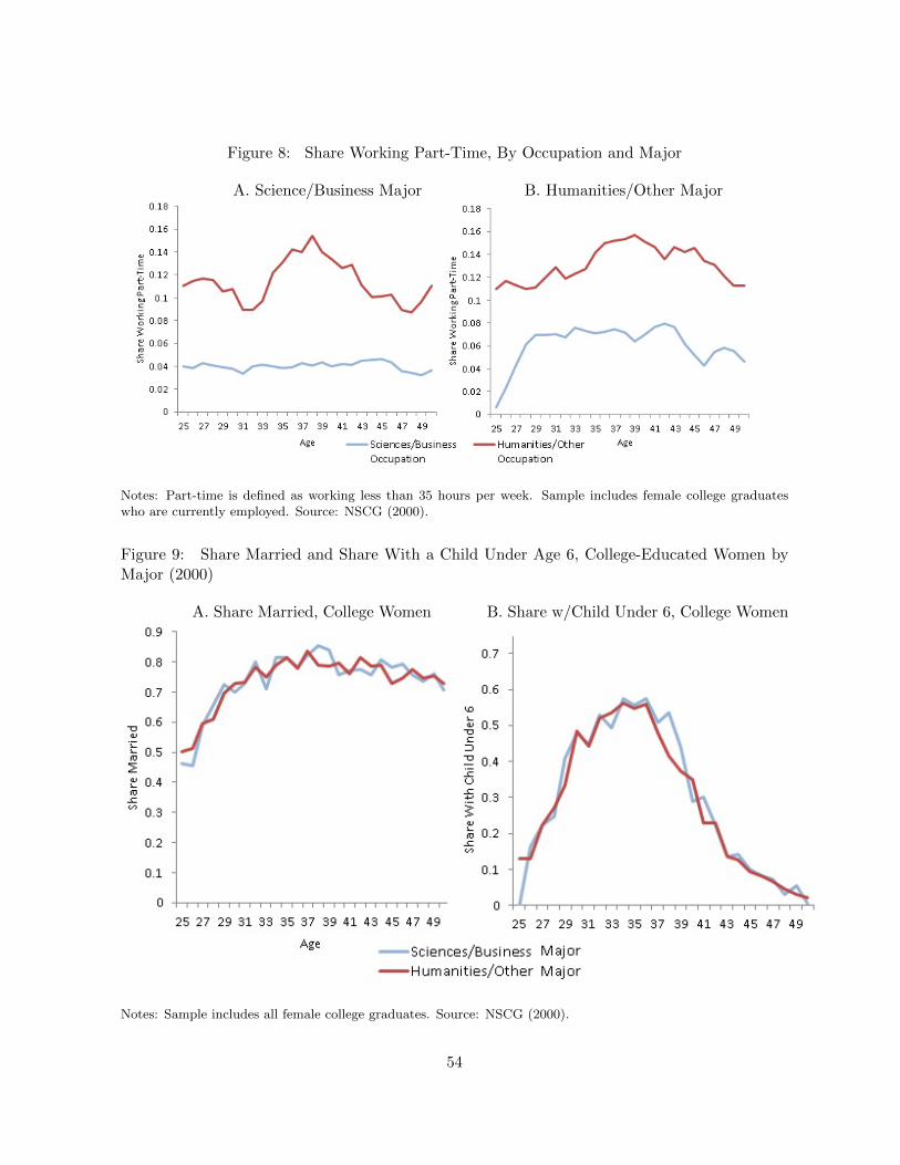
Figure 8: Share Working Part-Time, By Occupation and Major

A. Science/Business Major B. Humanities/Other Major

Notes: Part-time is defined as working less than 35 hours per week. Sample includes female college graduateswho are currently employed. Source: NSCG (2000).

Figure 9: Share Married and Share With a Child Under Age 6, College-Educated Women byMajor (2000)

A. Share Married, College Women B. Share w/Child Under 6, College Women

Notes: Sample includes all female college graduates. Source: NSCG (2000).

54

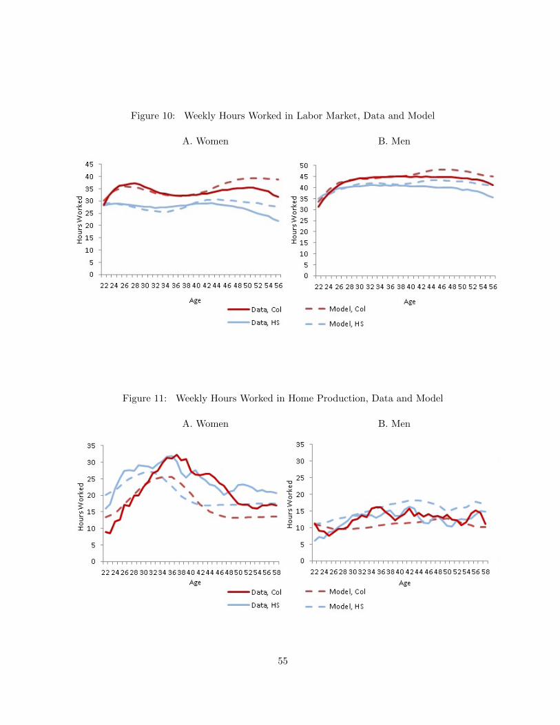
Figure 10: Weekly Hours Worked in Labor Market, Data and Model

A. Women B. Men

Figure 11: Weekly Hours Worked in Home Production, Data and Model

A. Women B. Men

55

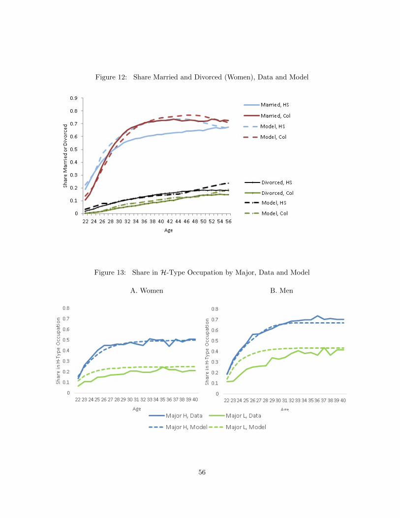
Figure 12: Share Married and Divorced (Women), Data and Model

Figure 13: Share in H-Type Occupation by Major, Data and Model

A. Women B. Men

56

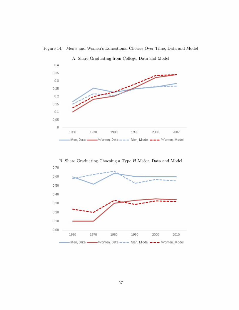
Figure 14: Men’s and Women’s Educational Choices Over Time, Data and Model

A. Share Graduating from College, Data and Model

B. Share Graduating Choosing a Type H Major, Data and Model

57

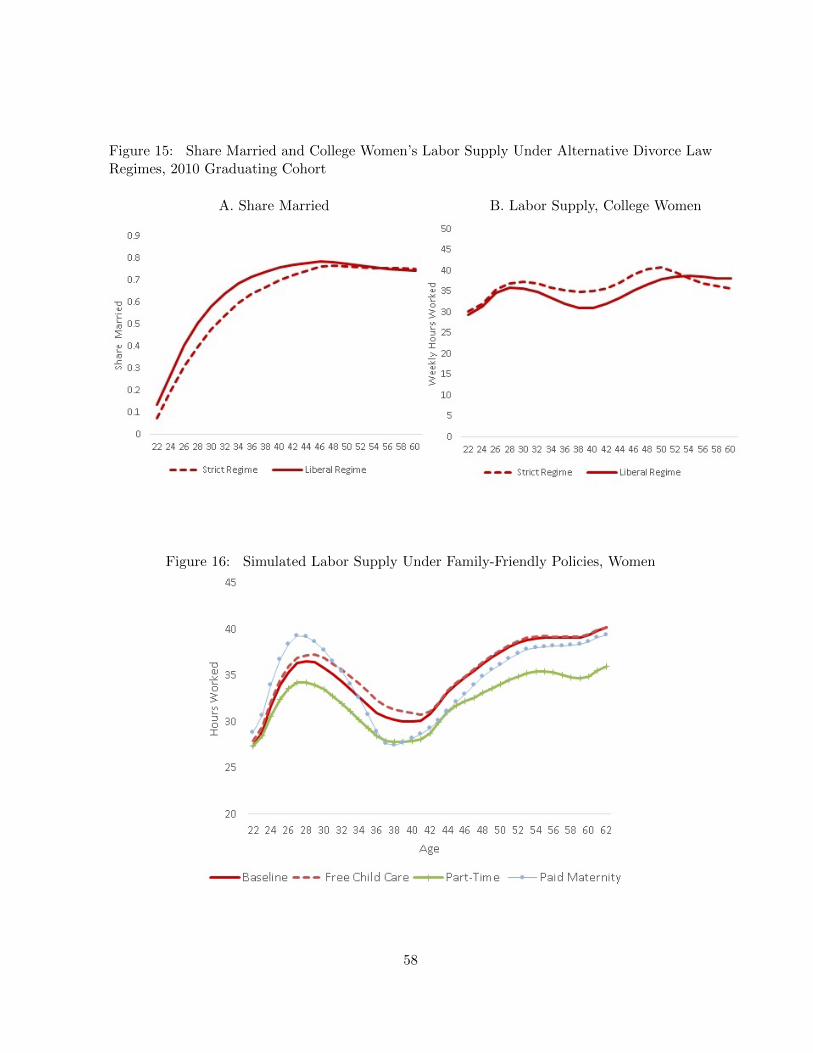
Figure 15: Share Married and College Women’s Labor Supply Under Alternative Divorce LawRegimes, 2010 Graduating Cohort

A. Share Married B. Labor Supply, College Women

Figure 16: Simulated Labor Supply Under Family-Friendly Policies, Women

58

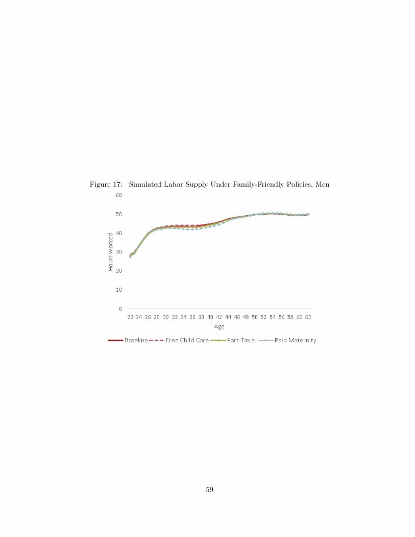
Figure 17: Simulated Labor Supply Under Family-Friendly Policies, Men

59

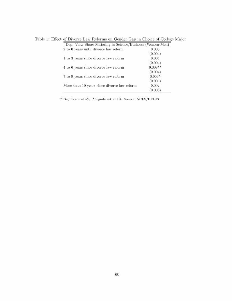
Table 1: Effect of Divorce Law Reforms on Gender Gap in Choice of College Major

Dep. Var.: Share Majoring in Science/Business (Women-Men)2 to 0 years until divorce law reform 0.003

(0.004)1 to 3 years since divorce law reform 0.005

(0.004)4 to 6 years since divorce law reform 0.008**

(0.004)7 to 9 years since divorce law reform 0.009*

(0.005)More than 10 years since divorce law reform 0.002

(0.008)

** Significant at 5%. * Significant at 1%. Source: NCES/HEGIS.

60

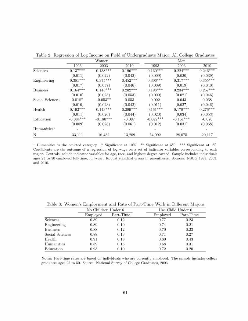
Table 2: Regression of Log Income on Field of Undergraduate Major, All College Graduates

Women Men1993 2003 2010 1993 2003 2010

Sciences 0.137*** 0.138*** 0.196*** 0.160*** 0.224*** 0.246***(0.011) (0.022) (0.042) (0.009) (0.020) (0.039)

Engineering 0.381*** 0.375*** 0.452*** 0.306*** 0.317*** 0.355***(0.017) (0.037) (0.046) (0.009) (0.019) (0.040)

Business 0.164*** 0.145*** 0.202*** 0.198*** 0.234*** 0.257***(0.010) (0.023) (0.053) (0.009) (0.021) (0.046)

Social Sciences 0.018* -0.053** 0.053 0.002 0.043 0.068(0.010) (0.023) (0.042) (0.011) (0.027) (0.046)

Health 0.192*** 0.143*** 0.299*** 0.161*** 0.179*** 0.276***(0.011) (0.026) (0.044) (0.020) (0.034) (0.053)

Education -0.084*** -0.180*** -0.097 -0.082*** -0.151*** -0.070(0.009) (0.028) (0.061) (0.012) (0.031) (0.068)

Humanities1 - - - - - -

N 33,111 16,432 13,209 54,992 28,075 20,117

1 Humanities is the omitted category. * Significant at 10%. ** Significant at 5%. *** Significant at 1%.Coefficients are the outcome of a regression of log wage on a set of indicator variables corresponding to eachmajor. Controls include indicator variables for age, race, and highest degree earned. Sample includes individualsages 25 to 50 employed full-time, full-year. Robust standard errors in parentheses. Sources: NSCG 1993, 2003,and 2010.

Table 3: Women’s Employment and Rate of Part-Time Work in Different Majors

No Children Under 6 Has Child Under 6Employed Part-Time Employed Part-Time

Sciences 0.89 0.12 0.77 0.23Engineering 0.89 0.10 0.74 0.21Business 0.88 0.12 0.70 0.23Social Sciences 0.88 0.13 0.71 0.27Health 0.91 0.18 0.80 0.43Humanities 0.89 0.15 0.68 0.31Education 0.93 0.10 0.72 0.20

Notes: Part-time rates are based on individuals who are currently employed. The sample includes collegegraduates ages 25 to 50. Source: National Survey of College Graduates, 2003.

61

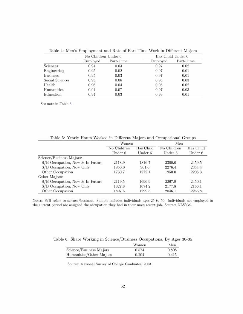
Table 4: Men’s Employment and Rate of Part-Time Work in Different Majors

No Children Under 6 Has Child Under 6Employed Part-Time Employed Part-Time

Sciences 0.94 0.03 0.97 0.02Engineering 0.95 0.02 0.97 0.01Business 0.95 0.03 0.97 0.01Social Sciences 0.93 0.06 0.96 0.03Health 0.96 0.04 0.98 0.02Humanities 0.94 0.07 0.97 0.03Education 0.94 0.03 0.99 0.01

See note in Table 3.

Table 5: Yearly Hours Worked in Different Majors and Occupational Groups

Women MenNo Children Has Child No Children Has Child

Under 6 Under 6 Under 6 Under 6Science/Business Majors:

S/B Occupation, Now & In Future 2118.9 1816.7 2300.0 2459.5S/B Occupation, Now Only 1850.0 961.0 2276.4 2354.4Other Occupation 1730.7 1272.1 1950.0 2205.3

Other Majors:S/B Occupation, Now & In Future 2119.5 1696.9 2267.9 2450.1S/B Occupation, Now Only 1827.8 1074.2 2177.8 2166.1Other Occupation 1897.5 1299.5 2046.1 2266.8

Notes: S/B refers to science/business. Sample includes individuals ages 25 to 50. Individuals not employed inthe current period are assigned the occupation they had in their most recent job. Source: NLSY79.

Table 6: Share Working in Science/Business Occupations, By Ages 30-35

Women MenScience/Business Majors 0.574 0.808Humanities/Other Majors 0.204 0.415

Source: National Survey of College Graduates, 2003.

62

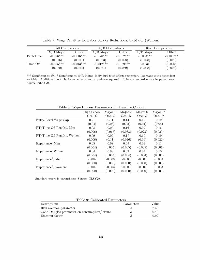
Table 7: Wage Penalties for Labor Supply Reductions, by Major (Women)

All Occupations S/B Occupations Other OccupationsS/B Major Other S/B Major Other S/B Major Other

Part-Time -0.126*** -0.116*** -0.178*** -0.162*** -0.083*** -0.108***(0.016) (0.011) (0.023) (0.028) (0.028) (0.028)

Time Off -0.105*** -0.043*** -0.212*** -0.159*** -0.031 -0.026*(0.020) (0.014) (0.031) (0.039) (0.028) (0.028)

*** Significant at 1%. * Significant at 10%. Notes: Individual fixed effects regression. Log wage is the dependentvariable. Additional controls for experience and experience squared. Robust standard errors in parentheses.Source: NLSY79.

Table 8: Wage Process Parameters for Baseline Cohort

High School Major L Major L Major H Major HOcc. L Occ. L Occ. H Occ. L Occ. H

Entry-Level Wage Gap 0.21 0.11 0.14 0.12 0.19(0.04) (0.03) (0.03) (0.04) (0.05)

PT/Time-Off Penalty, Men 0.08 0.09 0.16 0.09 0.16(0.006) (0.017) (0.033) (0.023) (0.020)

PT/Time-Off Penalty, Women 0.09 0.09 0.17 0.10 0.19(0.006) (0.11) (0.026) (0.06) (0.022)

Experience, Men 0.05 0.08 0.09 0.09 0.11(0.004) (0.005) (0.005) (0.005) (0.007)

Experience, Women 0.04 0.08 0.09 0.07 0.10(0.004) (0.003) (0.004) (0.004) (0.006)

Experience2, Men -0.002 -0.003 -0.003 -0.003 -0.003(0.000) (0.000) (0.000) (0.000) (0.000)

Experience2, Women -0.002 -0.003 -0.003 -0.003 -0.003(0.000) (0.000) (0.000) (0.000) (0.000)

Standard errors in parentheses. Source: NLSY79.

Table 9: Calibrated ParametersDescription: Parameter: ValueRisk aversion parameter σ 2.50Cobb-Douglas parameter on consumption/leisure a 0.40Discount factor β 0.92

63

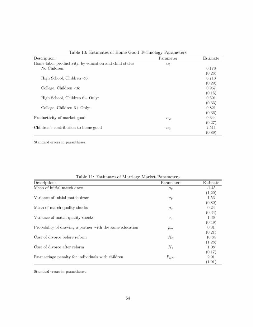
Table 10: Estimates of Home Good Technology Parameters

Description: Parameter: EstimateHome labor productivity, by education and child status α1

No Children: 0.178(0.28)

High School, Children <6: 0.713(0.29)

College, Children <6: 0.967(0.15)

High School, Children 6+ Only: 0.591(0.33)

College, Children 6+ Only: 0.821(0.36)

Productivity of market good α2 0.344(0.27)

Children’s contribution to home good α3 2.511(0.89)

Standard errors in parantheses.

Table 11: Estimates of Marriage Market Parameters

Description: Parameter: EstimateMean of initial match draw µθ -1.45

(1.20)Variance of initial match draw σθ 1.53

(0.80)Mean of match quality shocks µz 0.24

(0.34)Variance of match quality shocks σz 1.36

(0.49)Probability of drawing a partner with the same education pm 0.81

(0.21)Cost of divorce before reform K0 10.84

(1.28)Cost of divorce after reform K1 1.08

(0.17)Re-marriage penalty for individuals with children PRM 2.91

(1.91)

Standard errors in parantheses.

64

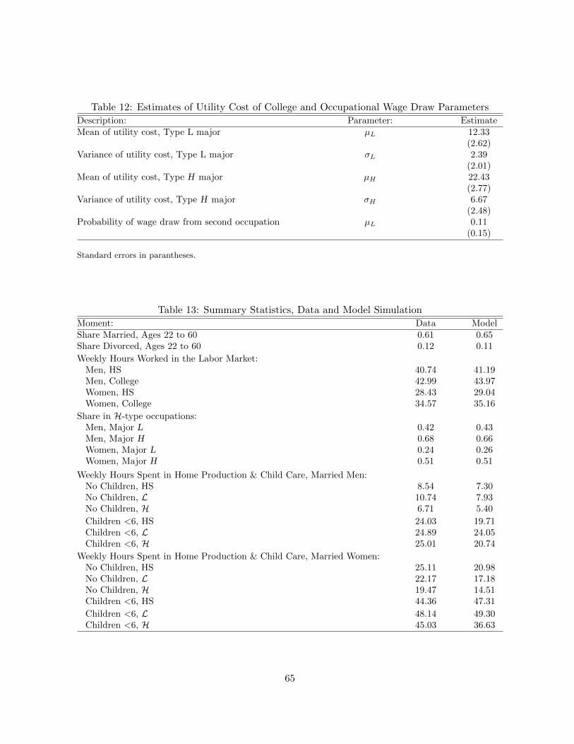
Table 12: Estimates of Utility Cost of College and Occupational Wage Draw Parameters

Description: Parameter: EstimateMean of utility cost, Type L major µL 12.33

(2.62)Variance of utility cost, Type L major σL 2.39

(2.01)Mean of utility cost, Type H major µH 22.43

(2.77)Variance of utility cost, Type H major σH 6.67

(2.48)Probability of wage draw from second occupation µL 0.11

(0.15)

Standard errors in parantheses.

Table 13: Summary Statistics, Data and Model Simulation

Moment: Data ModelShare Married, Ages 22 to 60 0.61 0.65Share Divorced, Ages 22 to 60 0.12 0.11

Weekly Hours Worked in the Labor Market:Men, HS 40.74 41.19Men, College 42.99 43.97Women, HS 28.43 29.04Women, College 34.57 35.16

Share in H-type occupations:Men, Major L 0.42 0.43Men, Major H 0.68 0.66Women, Major L 0.24 0.26Women, Major H 0.51 0.51

Weekly Hours Spent in Home Production & Child Care, Married Men:No Children, HS 8.54 7.30No Children, L 10.74 7.93No Children, H 6.71 5.40

Children <6, HS 24.03 19.71Children <6, L 24.89 24.05Children <6, H 25.01 20.74

Weekly Hours Spent in Home Production & Child Care, Married Women:No Children, HS 25.11 20.98No Children, L 22.17 17.18No Children, H 19.47 14.51Children <6, HS 44.36 47.31

Children <6, L 48.14 49.30Children <6, H 45.03 36.63

65

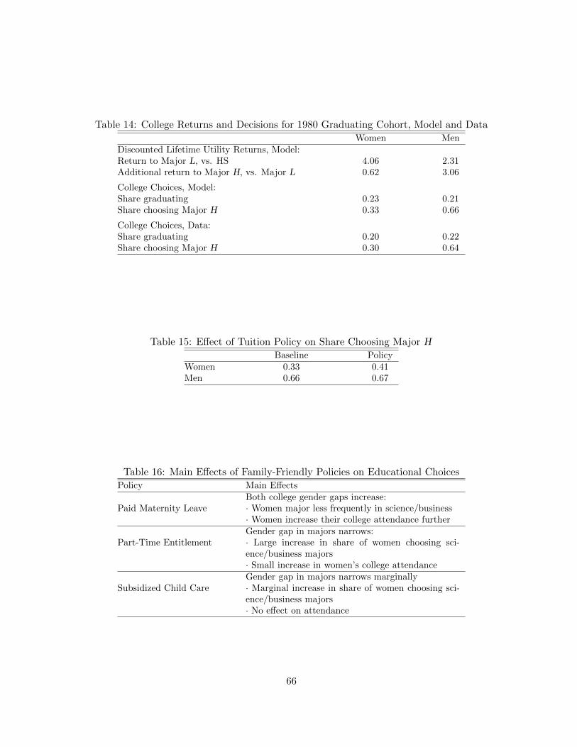
Table 14: College Returns and Decisions for 1980 Graduating Cohort, Model and Data

Women MenDiscounted Lifetime Utility Returns, Model:Return to Major L, vs. HS 4.06 2.31Additional return to Major H, vs. Major L 0.62 3.06

College Choices, Model:Share graduating 0.23 0.21Share choosing Major H 0.33 0.66

College Choices, Data:Share graduating 0.20 0.22Share choosing Major H 0.30 0.64

Table 15: Effect of Tuition Policy on Share Choosing Major H

Baseline PolicyWomen 0.33 0.41Men 0.66 0.67

Table 16: Main Effects of Family-Friendly Policies on Educational Choices

Policy Main Effects

Paid Maternity LeaveBoth college gender gaps increase:· Women major less frequently in science/business· Women increase their college attendance further

Part-Time EntitlementGender gap in majors narrows:· Large increase in share of women choosing sci-ence/business majors· Small increase in women’s college attendance

Subsidized Child CareGender gap in majors narrows marginally· Marginal increase in share of women choosing sci-ence/business majors· No effect on attendance

66