Embed Size (px)
Citation preview
DÉBORA VIANA E SOUSA PEREIRA
AN ANALYSIS OF HOMICIDES IN RECIFE, BRAZIL
A thesis presented to the Federal University of
Pernambuco to the achievement of PhD degree as part
of the requirements from Postgraduate Program in
Production Engineering (Main area: Production
management).
Supervisor: Caroline Maria de Miranda Mota, PhD.
Co-supervisor: Martin Alexander Andresen, PhD.
Recife
2016
Catalogação na fonte
Bibliotecária Valdicèa Alves, CRB-4 / 1260
P429a Pereira, Débora Viana e Sousa.
An analysis of homicides in Recife, Brazil. / Débora Viana e
Sousa. - 2016.
165folhas, Il., Tab., Abr. e Equa.
Orientadora: Profª. DSc. Caroline Maria de Miranda Mota,
Coorientador: Profº Martin Alexander Andresen.
Tese (Doutorado) – Universidade Federal de Pernambuco. CTG.
Programa de Pós-Graduação Engenharia de produção, 2016.
Inclui Referências.
Nota: Texto bilíngue.
1. Engenharia de produção. 2. Homicídios. 3. Análise temporal .
4. Análise especial. 5. Análise ambiental. 6. Teoria da
desorganização social. I. Mota. Caroline Maria de
Miranda(Orientadora). II. Andresen, Martin Alexander(Coordenador).
III. Título.

For my true love, Marília.
ACKNOWLEDGMENT
Primeiramente gostaria de agradecer a Deus pelas grandes oportunidades que tive até
aqui. Sei que esse sonho não teria sido concretizado sem o apoio Dele. Ele permitiu que logo
cedo eu descobrisse a minha vocação e que eu encontrasse pessoas maravilhosas que me
ajudaram nessa jornada.
Gostaria de agradecer à minha irmã Marília, que me incentiva e inspira. Ela sempre teve
as palavras certas nos momentos difíceis, me ajudando a seguir em frente. Meus pais, Adriana
e César, também devem ser lembrados. Sem eles eu não teria chegado tão longe. Ambos sempre
prezaram pela minha educação e me deram suporte na minha caminhada. Agradeço ainda à
minha família, que sempre acompanhou o desenvolvimento do meu trabalho. Foram muitas
orações, algumas preocupações, muita força e vários momentos de entusiasmo.
Meu período de doutoramento também foi marcado pela presença dos meus amigos. Aos
amigos do PPGEP, agradeço a companhia do dia-a-dia. Gostaria de agradecer a Thárcylla,
Creuza e Ciro. Meus amigos da vida também foram importantes, pois me apoiaram moralmente
e entenderam a minha ausência. Agradeço especialmente a Leandro, que esteve muito presente
na reta final dessa minha jornada. Também preciso agradecer àqueles amigos que foram minha
família durante o doutorado sanduíche: Leila, Paulo, Renata e André.
Meu agradecimento à Carol, minha orientadora, com quem tenho o prazer de trabalhar
desde o mestrado. Eu tenho profundo respeito e admiração por ela e reconheço que os seus
conselhos me trouxeram até aqui.
I need to thank my co-supervisor, Martin Andresen. He has a brilliant mind and I learned
a lot with him. He is the most patient and talented person that I have ever met. I do not have
words to say how grateful I am for the opportunity of work with him.
My friends from Simon Fraser University were very important to me. Silas, Ashley,
Adam, Amir, Shannon, Allison, and Kate: Thank you for all the support. I have to thank Mary
Williams, my first friend in Vancouver. She is a lovely and generous person. I will not forget
everything she made to me.
Agradeço à banca pelas contribuições dadas ao meu trabalho. Também quero dizer
obrigada às pessoas que trabalham na secretaria do PPGEP, em especial à Poliana. Meus
agradecimentos ainda à Facepe, ao Capes e à SEPLAG, pelo apoio financeiro concedido
durante o doutoramento.
ABSTRACT
In Brazil, since 2000, approximately 50,000 people are murdered every year. In a span of 30
years (1980 – 2010), more than 1 million homicides were registered. In 2012, the homicide rate
in Brazil was 29 homicides per 100,000 inhabitants. All Brazilian states exceed the threshold
of epidemic established by World Health Organization. In this context, the present study has
the objective of to investigate homicides in Recife, taking into account temporal, spatial,
environmental, and multicriteria analysis. The temporal analysis shows that the difference of
homicides between seasons and months is not statistically significant. However, there is a
significant increase in homicides during the weekends (42 percent of all homicides) and
evenings (62 percent). Moreover, the spatial results show that the spatial patterns are different
within the temporal dimensions in many cases. The findings from spatial analysis reveal that
homicides are very concentrated in the city of Recife and in a time span of five years (2009-
2013) all the homicides occurred in less than 10 percent of the street segments. In addition, our
test showed that the spatial pattern was not stable over the years. However, when we consider
the temporal dimensions (as suggested by temporal analysis), the patterns were stable along the
years – except for weekdays and night/dawn. Furthermore, through the environmental analysis,
we found that inequality, rented houses, and number of residents have a positive relationship
with homicide. On the other hand, income, education, public illumination, population density,
and street network density have a negative relationship. The findings of these analyses indicate
that homicide in Recife can be understood by the perspective of social disorganization theory
and routine activity theory. Finally, multicriteria approach was applied to highlight vulnerable
areas to homicide in Recife. We considered six variables to evaluate vulnerability and the areas
were identified by PROMETHEE II method and local Moran’s I. Other application was made
in Boa Viagem neighborhood, so we were able to perform a more detailed analysis. Three
different approaches were tested for Boa Viagem and we suggested some actions in order to
reduce criminality in long term.
Keywords: Homicide. Temporal analysis. Spatial analysis. Environmental analysis. Social
disorganization theory. Routine activity theory. Multicriteria decision aid. Vulnerability.
RESUMO
No Brasil, desde 2000, aproximadamente 50,000 foram mortas todos os anos. Em um espaço
de 30 anos (1980 – 2000), mais de 1 milhão de homicídios foram registrados. Em 2012, a taxa
de homicídio no Brasil era 29 homicídios para cada 100,000 habitantes. Todos os estados
brasileiros excedem o limite de epidemia estabelecido pela Organização Mundial de Saúde.
Nesse contexto, o presente estudo tem o objetivo de investigar os homicídios em Recife,
levando em consideração análises temporal, espacial, ambiental e multicritério. A análise
temporal mostra que a diferença de homicídios entre estações do ano e meses não é
estatisticamente significativa. Porém, existe um aumento significante de homicídios durante os
finais de semana (42 por cento de todos os homicídios) e noites (62 por cento). E ainda, os
resultados espaciais mostram que os padrões espaciais são diferentes dento das dimensões
temporais em muitos casos. Os achados da análise espacial revelam que homicídios são muito
concentrados na cidade do Recife e que em um espaço de tempo de cinco anos (2009-2013)
todos os homicídios ocorreram em menos de 10 por cento dos segmentos de rua. E ainda, o
teste do padrão dos pontos espaciais mostrou que os padrões espaciais não foram estáveis no
decorrer dos anos. Porém, quando se considera das dimensões temporais (como sugerido pela
análise temporal), os padrões foram estáveis ao longo dos anos – com exceção de dias de
semana e noites/madrugadas. Além disso, através da análise ambiental encontrou-se que
desigualdade, casas alugadas e número de residentes têm uma relação positiva com homicídio.
Por outro lado, renda, educação, iluminação pública, densidade populacional e densidade da
rede de ruas têm uma relação negativa. Os achados dessas análises indicam que os homicídios
em Recife podem ser entendidos pela perspectiva da teoria da desorganização social e da teoria
das atividades de rotina. Finalmente, abordagem multicritério foi aplicada para destacar áreas
vulneráveis aos homicídios em Recife. Considerou-se seis variáveis para avaliar a
vulnerabilidade e as áreas foram identificados pelo PROMETHEE II e pelo índice local de
Moran. Outra aplicação foi feita no bairro de Boa Viagem e foi possível realizar uma análise
mais detalhada. Três diferentes abordagens foram testadas para Boa Viagem e sugeriu-se
algumas ações no sentido de reduzir a criminalidade no longo prazo.
Palavras-chave: Homicídios. Análise temporal. Análise espacial. Análise ambiental. Teoria da
desorganização social. Teoria das atividades de rotina. Apoio multicritério à decisão.
Vulnerabilidade.
LIST OF FIGURES
Figure 4.1 - Historical trend of homicides in Brazil ................................................................. 51
Figure 4.2 - Variation of homicides in Brazil by region (2002 – 2012) ................................... 53
Figure 4.3 - Variation of homicides in Brazil by state (2002 – 2012) ...................................... 54
Figure 4.4 - Historical trend of homicides in Pernambuco....................................................... 56
Figure 4.5 - Historical trend of homicides in Metropolitan Region of Recife ......................... 57
Figure 4.6 - Monthly trend of homicides in Metropolitan Region of Recife ........................... 58
Figure 4.7 - Overall trends of homicide rates ........................................................................... 59
Figure 5.1 - Temperature variation in Recife by month (2009 to 2013) .................................. 67
Figure 6.1 - Histograms of number of homicides per census tract in the city of Recife .......... 83
Figure 8.1 - Net outranking flows of all census tracts from RMR ......................................... 113
Figure 8.2 - Vulnerability clusters and outliers from RMR ................................................... 114
Figure 8.3 - Boxplots, cluster and outlier analysis ................................................................. 115
Figure 8.4 - Details of high-high clusters ............................................................................... 117
Figure 8.5 - Details of low-low clusters ................................................................................. 119
Figure 9.1 - Location of Boa Viagem neighborhood.............................................................. 123
Figure 9.2 - Results from first approach ................................................................................. 125
Figure 9.3 - Division of Boa Viagem into 13 groups ............................................................. 126
Figure 9.4 - Results from second approach ............................................................................ 128
Figure 9.5 - Results from third approach ................................................................................ 129
Figure 9.6 - Boxplots of group 12 (1st in the ranking) ............................................................ 131
Figure 9.7 - Details of group 12 ............................................................................................. 132
Figure 9.8 - Boxplots of group 4 (2nd in the ranking) ............................................................. 132
Figure 9.9 - Details of group 4 ............................................................................................... 133
Figure 9.10 - Boxplots of group 5 (3rd in the ranking) ........................................................... 133
Figure 9.11- Details of group 5 .............................................................................................. 134
Figure 9.12 - Boxplots of group 9 (4th in the ranking) ........................................................... 134
Figure 9.13 - Details of group 9 ............................................................................................. 135
Figure 9.14 - Boxplots of group 6 (5th in the ranking) ........................................................... 135
Figure 9.15 - Details of group 6 ............................................................................................. 136
Figure 9.16 - Performances on income ................................................................................... 136
Figure 9.17 - Performances on inequality .............................................................................. 137
Figure 9.18 - Performances on education ............................................................................... 137
Figure 9.19 - Performances on public illumination ................................................................ 138
Figure 9.20 - Performances on population density ................................................................. 138
Figure 9.21 - Performances on rented houses ......................................................................... 139
LIST OF TABLES
Table 2.1 - Types of criteria ..................................................................................................... 27
Table 4.1 - Homicide rates in Brazilian states, 2012 ................................................................ 55
Table 4.2 - Intentional lethal violent crime rates in Pernambuco ............................................. 60
Table 4.3 - Pact for Life projects and PST model .................................................................... 62
Table 5.1 - Count and percentage of homicides by temporal units .......................................... 68
Table 5.2 - Results from ANOVA ............................................................................................ 69
Table 5.3 - Similarity index of homicides in Recife by seasons .............................................. 70
Table 5.4 - Similarity index of homicides in Recife by months ............................................... 71
Table 5.5 - Similarity index of homicides in Recife by days of week ..................................... 71
Table 5.6 - Similarity index of homicides in Recife by periods of day .................................... 71
Table 5.7 - Similarity index of homicides in Recife by weekday versus weekend .................. 72
Table 5.8 - Similarity index of homicides in Recife by day versus night ................................ 72
Table 6.1 - Homicides in the city of Recife by census tracts ................................................... 82
Table 6.2 - Percentages of homicides in the city of Recife ...................................................... 84
Table 6.3 - Results of spatial point pattern test by year ........................................................... 86
Table 6.4 - Results of spatial point pattern test by season ........................................................ 87
Table 6.5 - Results of spatial point pattern test by month ........................................................ 88
Table 6.6 - Results of spatial point pattern test by days of week ............................................. 88
Table 6.7 - Results of spatial point pattern test by periods of day ........................................... 88
Table 6.8 - Results of spatial point pattern test by weekday versus weekend .......................... 89
Table 6.9 - Results of spatial point pattern test by day versus night ........................................ 89
Table 7.1 - Descriptive statistics, Recife, 2010 ...................................................................... 100
Table 7.2 - Spatial regression results ...................................................................................... 102
Table 7.3 - Spatial regression results, full model ................................................................... 103
Table 8.1 - Parameters for PROMETHEE II .......................................................................... 112
Table 8.2 - Descriptive statistics, cluster and outlier analysis ................................................ 115
Table 8.3 - Comparison among the groups, cluster and outlier analysis ................................ 116
Table 9.1 - Positions and net outranking flows of each group ............................................... 131
LIST OF EQUATIONS
Equation (2.1) - Similarity index .............................................................................................. 23
Equation (2.2) - Relation of preference .................................................................................... 25
Equation (2.3) - Relation of indifference.................................................................................. 25
Equation (2.4) - Relation of incomparability............................................................................ 25
Equation (2.5) - Preference function ........................................................................................ 26
Equation (2.6) - Preference index ............................................................................................. 28
Equation (2.7) - Positive outranking flow ................................................................................ 29
Equation (2.8) - Negative outranking flow ............................................................................... 29
Equation (2.9) - Net outranking flow ....................................................................................... 29
Equation (2.10) - Rules for PROMETHEE II ranking ............................................................. 29
Equation (2.11) - Spatial error model ....................................................................................... 32
Equation (2.12) - Local Moran’s I ............................................................................................ 34
Equation (7.1) - Blau’s heterogeneity index ............................................................................. 96
LIST OF ABBREVIATIONS
CT – Census tract
DATASUS – (Departamento de Informática do Sistema Único de Saúde, in Portuguese) IT
Departament of Health Unic System
GDP – Gross Domestic Product
HH – High-high cluster
HL – High-low outlier
IBGE – (Instituto Brasileiro de Geografia e Estatística, in Portuguese) Brazilian Institute of
Geography and Statistics
ICE – Index of Concentration at the Extremes
ICPC – International Centre for the Prevention of Crime
ILVC – Intentional lethal violent crime
INMET – (Instituto Nacional de Meteorologia, in Portuguese) National Institute of
Meteorology
IPEA – (Instituto de Pesquisa Econômica Aplicada, in Portuguese) Institute for Applied
Economic Research
LH – Low-high outlier
LL – Low-low cluster
MCDA – Multicriteria Decision Aid
MRR – Metropolitan Region of Recife
PFL – Pact for Life
PROMETHEE – Preference Ranking Organization Method for Enrichment Evaluation
PST model – Primary, Secondary, and Tertiary model
SDS – (Secretaria de Defesa Social, in Portuguese) Secretariat of Social Defense
SPPT – Spatial Point Pattern Test
UNODC – United Nations Office on Drugs and Crime
CONTENTS
1 Introduction ............................................................................................................ 14
1.1 Justification ....................................................................................................... 16
1.2 Purposes ............................................................................................................ 17
1.2.1 General purpose ............................................................................................ 17
1.2.2 Specific purposes .......................................................................................... 17
1.3 Structure of this thesis ...................................................................................... 18
2 Data and method ..................................................................................................... 20
2.1 Area of study .................................................................................................... 20
2.2 Units of analysis ............................................................................................... 20
2.3 Homicide data ................................................................................................... 21
2.4 Census variables ............................................................................................... 22
2.5 Methods ............................................................................................................ 22
2.5.1 Spatial Point Pattern Test ............................................................................. 22
2.5.2 Multicriteria decision aid .............................................................................. 24
2.5.2.1 PROMETHEE family ............................................................................ 25
2.5.2.2 PROMETHEE II .................................................................................... 28
2.5.3 Temporal analysis ......................................................................................... 29
2.5.4 Spatial analysis ............................................................................................. 31
2.5.5 Environmental analysis................................................................................. 31
2.5.6 Multicriteria analysis .................................................................................... 33
2.5.6.1 Application in Metropolitan Region of Recife ....................................... 33
2.5.6.2 Application in Boa Viagem neighborhood ............................................ 34
2.6 Final comments................................................................................................. 35
3 Theoretical background and literature review .................................................... 36
3.1 Theories about crime ........................................................................................ 36
3.1.1 Social disorganization theory ....................................................................... 36
3.1.2 Routine activity theory ................................................................................. 38
3.2 Homicide and temporal variation ..................................................................... 39
3.2.1 Previous research on temporal variations of homicide ................................. 40
3.2.2 Previous research on temporal variation of homicide in Brazil ................... 41
3.3 Homicide and space .......................................................................................... 43
3.4 Homicide and environmental factors ................................................................ 45
3.4.1 Recent research on homicide and environmental factors ............................. 45
3.4.2 Recent research on homicide and environmental factors in Brazil .............. 47
3.5 Final comments................................................................................................. 50
4 Homicide in Brazil, Pernambuco, and Recife ...................................................... 51
4.1 Homicide in Brazil............................................................................................ 51
4.2 Homicide in Pernambuco ................................................................................. 55
4.3 Homicide in Metropolitan Region of Recife .................................................... 57
4.4 Comparison of homicides in Brazil, Pernambuco, and Recife ......................... 58
4.5 Pact for Life Program ....................................................................................... 59
4.6 Final comments................................................................................................. 62
5 Temporal analysis of homicide in Recife .............................................................. 64
5.1 Contextualization .............................................................................................. 64
5.2 Purpose of temporal analysis ............................................................................ 66
5.3 Recife’s climate ................................................................................................ 66
5.4 Results .............................................................................................................. 67
5.4.1 Descriptive results ........................................................................................ 67
5.4.2 ANOVA results ............................................................................................ 69
5.4.3 Spatial results ................................................................................................ 70
5.5 Discussion ......................................................................................................... 73
5.5.1 Temporal aggression theory versus routine activity theory.......................... 73
5.5.2 Temporal variation ....................................................................................... 74
5.5.3 Spatial variation ............................................................................................ 77
5.6 Final comments................................................................................................. 79
6 Spatial analysis of homicide in Recife ................................................................... 80
6.1 Contextualization .............................................................................................. 80
6.2 Purpose of spatial analysis ................................................................................ 81
6.3 Results .............................................................................................................. 82
6.3.1 Descriptive statistics ..................................................................................... 82
6.3.2 Homicide concentrations .............................................................................. 84
6.3.3 Stability of spatial concentrations................................................................. 85
6.4 Discussion ......................................................................................................... 90
6.5 Final comments................................................................................................. 93
7 Environmental analysis of homicide in Recife ..................................................... 94
7.1 Contextualization .............................................................................................. 94
7.2 Purpose of environmental analysis ................................................................... 95
7.3 Environmental variables ................................................................................... 95
7.4 Results and discussion ...................................................................................... 99
7.4.1 Descriptive results ........................................................................................ 99
7.4.2 Inferential results ........................................................................................ 101
7.5 Final comments............................................................................................... 107
8 Identifying vulnerable areas to homicide in Recife ........................................... 108
8.1 Contextualization ............................................................................................ 108
8.2 Purpose of this chapter ................................................................................... 111
8.3 Application ..................................................................................................... 111
8.4 Results and discussion .................................................................................... 112
8.5 Final comments............................................................................................... 120
9 Identifying vulnerable areas to homicide in Boa Viagem neighborhood ........ 122
9.1 Purpose of this chapter ................................................................................... 122
9.2 Application ..................................................................................................... 123
9.2.1 Identifying vulnerable areas to homicide in Boa Viagem – 1st approach ... 124
9.2.1 Identifying vulnerable areas to homicide in Boa Viagem – 2nd approach .. 125
9.2.1 Identifying vulnerable areas to homicide in Boa Viagem – 3rd approach .. 127
9.3 Results and discussion .................................................................................... 130
9.4 Final comments............................................................................................... 143
10 Final remarks ........................................................................................................ 145
10.1 Conclusions .................................................................................................... 145
10.1.1 Temporal analysis ................................................................................... 145
10.1.2 Spatial analysis ....................................................................................... 146
10.1.3 Environmental analysis........................................................................... 146
10.1.4 Multicriteria analysis .............................................................................. 147
10.2 Implications of this study ............................................................................... 148
10.3 Limitations ...................................................................................................... 149
10.4 Suggestions for future works .......................................................................... 151
References ................................................................................................................... 152
Chapter 1 Introduction
14
1 INTRODUCTION
Violent deaths in developing countries is a known and old problem. According to United
Nations Office on Drugs and Crime (UNODC) (UNODC, 2013), the regions with higher
homicide rates are Southern Africa, Central America, South America, Middle Africa, and the
Caribbean – all of them with homicide rates above than 16 homicides per 100,000 inhabitants.
Brazil has higher homicide rate than the most populous countries in the world such as China,
India, United States, Indonesia, Pakistan, Nigeria, Bangladesh, Russia, Japan, and Mexico
(Waiselfisz, 2013). Brazil is more similar to countries like South Africa according to its levels
of violence (Breetzke, 2010).
Considering 2012, 10 percent of homicides in the world occurred in Brazil, while this
country has less than 3 percent of the world’s population (UNODC, 2013). In Brazil, since
2000, approximately 50,000 people are murdered every year. In a span of 30 years (1980 –
2010), more than 1 million homicides were registered in Brazil (Waiselfisz, 2012). This is an
incredible magnitude of homicides, even more if we consider that Brazil is a country that does
not have conflicts of religion, ethnicity, race, or territory. It is important to notice that all the
Brazilian states exceed the threshold for epidemic established by World Health Organization of
10 homicides per 100,000 inhabitants (United Nations Development Programme, 2013).
In 2012, the homicide rate in Brazil was 29 homicides per 100,000 inhabitants
(Waiselfisz, 2014). This rate, however, varies significantly across the country: among the state
capitals we can find rates between 12.8 (Santa Catarina) and 64.6 (Alagoas) (Waiselfisz, 2014).
Moreover, the homicide trend is not the same across Brazil: while few states are experiencing
a homicide drop, other states are experiencing an increase. Rio Grande do Norte and Bahia, for
example, more than doubled their homicide rates in the past decade, while São Paulo, Rio de
Janeiro, and Pernambuco had significant decreases (Waiselfisz, 2014).
Although Brazil had made many efforts to reduce crime in recent years, the number of
homicides is growing again. In 2002, the country had a homicide rate of 28.5 per 100,000
inhabitants, with a small decrease to 25.2 per 100,000 inhabitants in 2007. After 2007, however,
Brazil had an increase in its homicide rate, reaching 29 homicides per 100,000 inhabitants in
2012 (Waiselfisz, 2014).
The Institute for Applied Economic Research (IPEA) – a Brazilian federal public
foundation – published a report that showed the feelings of personal security in Brazil: 62.4
Chapter 1 Introduction
15
percent of Brazilians declared to have an intense fear of being murdered and 23.2 percent
claimed to have some level of fear (IPEA, 2012). In the northeast region, however, the situation
is the worst in Brazil: 72.9 percent of the population has an intense fear of being murdered and
19.9 percent has some level of fear (IPEA, 2012). This same report indicates the causes of
criminality in Brazil, according to the population, to be social and economic inequality (23.8
percent) and a lack of investment in education (20.5 percent).
These numbers show that the Brazilian scenario regarding homicides is very alarming.
Something needs to be done in order to change the present trend of homicide and try to decrease
the homicide rate to an acceptable level. Of course, it is unreasonable to attempt to prevent all
homicides, but something needs to be done to save the majority of the 50,000 lives that are
being lost every year. We believe that the first step in order to combat homicides is a better
understanding about the problem.
In this sense, this work aimed to thoroughly investigate the homicides within
Metropolitan Region of Recife. In this thesis, we show the study of temporal, spatial, and
environmental characteristics of homicides in Recife between 2009 and 2013. Furthermore, we
applied multicriteria approach in order to identify the most vulnerable areas in Recife and the
Boa Viagem neighborhood. The results from temporal analysis reveal that there is statistically
significant temporal variation of homicides for days of week and periods of day. Moreover, the
findings show that the spatial patterns are not similar when we consider different temporal units.
Another conclusion of this analysis is that homicides in Recife can be understood according to
routine activity theory.
The spatial analysis revealed that homicides are highly concentrated in the city of Recife
and they occurred in fewer than 10 percent of the street segments during 2009 and 2013. The
spatial analysis also showed that homicides were not stable over years but it presents stability
when we take into account temporal dimensions – except for weekdays and night/dawn. Finally,
the environmental analysis showed the determinants of homicide in Recife and concluded that
this phenomenon can be understood by social disorganization theory. The regression analysis
indicated that factors such as income, income inequality, education, public illumination,
density, and rented houses are related to homicides in Recife.
The multicriteria analysis was useful to identify the most vulnerable areas regarding
homicides. For Recife, we considered six variables to evaluate vulnerability and the areas were
identified by PROMETHEE II method and local Moran’s I. Another application was made in
Chapter 1 Introduction
16
Boa Viagem neighborhood, so we were able to perform a more detailed analysis. Overall, we
found five hot spots and three cold spots in Boa Viagem and we suggested some actions in
order to reduce homicide in the long term.
The findings of this study are important because they bring implications for theory and
policy. The results reveal significant details about homicides in Recife and they should be taken
into account in the development of new researches and in the elaboration of public policy.
1.1 Justification
We think it is important to highlight the motivations for this work. I (Débora) am
personally involved with this study because it is about peoples’ lives and I think it is useful for
the community – through this work we can have a better understanding about the dynamics of
homicide and then search for actions that are more efficient to prevent homicide. But why did
I decide to investigate homicides?
The first reason is that homicides involve a tragic end: somebody’s death. When a
homicide occurs, it means that one life is gone and the human capital was affected. Beyond all
the pain of the families, homicides are also responsible for reduction in quality of life, decreases
of touristic interest, and the loss of economic investments. I do not feel comfortable with this
situation and, as a researcher, I think I need to do something to avoid more deaths.
Another idea that makes me uncomfortable is the epidemic situation of Brazil regarding
to homicides. The World Health Organization established a threshold of 10 homicides per
100,000 inhabitants to consider a country as having an epidemic status (United Nations
Development Programme, 2013). Therefore, I think that we Brazilians need to do something to
change this reality – it is a shame.
In addition, homicides are affecting an important group: the youth. Homicides are the
main cause of death among youths when we consider external causes. According to DATASUS
(2015), 56.76 percent of the external deaths of people between 15 and 19 years old were
homicides (considering all Brazil in 2011). This number is 53.24 percent for people between
20 and 24 years old and 50.55 percent for 25 and 29 years old (DATASUS, 2015). Faced with
these numbers, we can conclude that our youth are being killed, so something needs to be done
in the sense of stopping it.
Moreover, I chose to work with homicides because this crime is more accurate than other
crime types. Sub notification is a notable problem when we study crime because it is known
Chapter 1 Introduction
17
that many victims do not register the occurrences. However, sub notification is not a big
problem when we are dealing with homicide. The nature of this crime implies that there is a
"disappearance" of someone and, most often, a dead body, so the majority of homicides are
reported to the police. Therefore, there is a benefit in working with homicides: we have minimal
problems about sub notification. Furthermore, it is easier to work with homicides, in Brazil,
because there is a national database that involves this crime. However, for others types of crime,
there is not a source to collect data.
Another motivation for this study was the intention of contribute with a lack in the
literature. Works regarding homicide and space are not common, especially in a Brazilian
context. In addition, we have the purpose of conduct a comprehensive analysis of homicides,
involving different dimensions and tools.
Finally, I want to explain why I am developing our studies in Recife. Firstly, Recife is the
city that I come from. Therefore, I know about the dynamics of this city and I have a particular
desire of improve the quality of life of my place. Second, Recife is an interesting case of study
because this city recently experienced a homicide drop. During 2009 and 2013, the number of
homicides in Metropolitan Region of Recife decreased almost 34 percent (SDS, 2014). In
addition, there is an excellent database about homicides in Pernambuco. Since June of 2008,
the Secretariat of Social Defense is collecting geographical coordinates of all homicides in
Recife, and it helps with future analysis.
1.2 Purposes
1.2.1 General purpose
The main purpose of this thesis is to realize a detailed study of homicides occurred in
Recife, taking into account temporal, spatial, environmental, and multicriteria analyses.
1.2.2 Specific purposes
The specific purposes of this thesis are:
To show an overview about homicides occurred in Brazil, Pernambuco, and
Recife;
To realize a temporal analysis of homicides in Recife, investigating the existence
of temporal variations;
Chapter 1 Introduction
18
To develop a spatial analysis of homicides in Recife, in order to investigate the
stability or not of spatial patterns over time;
To study the environmental factors that can be related to homicides in Recife;
To verify which theories can explain the phenomenon of homicides in Recife; and
To perform a multicriteria analysis to identify the most vulnerable areas regarding
homicides in Recife.
1.3 Structure of this thesis
This thesis is divided in ten chapters.
The next chapter (second) is about the datasets and the methods that were employed in
this work. Firstly, we comment about the area of study, the Metropolitan Region of Recife.
After, we talk about the source of homicide and socioeconomic datasets. We also present the
Spatial Point Patter Test and Multicriteria Decision Aid approach. Finally, we speak separately
about the methodology of each analysis – temporal, spatial, environmental, and multicriteria.
The third chapter is aimed to show the theoretical background and literature review.
Therefore, we speak about some theories related to crime and we present many works about
temporal, spatial, and environmental analysis of homicide.
The fourth chapter has the objective of exhibit an overview about homicide in Recife,
Pernambuco, and Brazil. In addition, this chapter discuss about Pact for Life Program.
Chapter five is about the temporal analysis of homicides in Recife. Here, we show the
results of temporal variation across seasons, months, days of week, and periods of day.
Furthermore, we performed a spatial analysis considering all these temporal dimensions. We
also comment about the link between our results and routine activity theory.
The sixth chapter shows the spatial analysis of homicides in Recife. We discuss about
crime concentration and the stability (or not) of the spatial patterns in Recife between 2009 and
2013, considering census tracts and street segments.
Chapter 7 is related to the environmental analysis of homicides in Recife. We show the
results of the spatial regression performed with 29 social, economic, and demographic
variables. In this chapter we relate our results with social disorganization theory.
Next, chapter 8 presents a preliminary attempt to identify vulnerable areas to homicide in
Recife. In this sense, we applied PROMETHEE II method and local Moran’s I to detect the
most vulnerable areas in Recife, according to some socioeconomic and demographic variables.
Chapter 1 Introduction
19
The following chapter (ninth) brings a similar analysis specifically in Boa Viagem
neighborhood, allowing a more detailed study. The difference of this analysis is that it is more
complete because we suggest some actions that can be taken in order to reduce criminality in
long term.
Finally, chapter ten brings the last comments about the analysis of homicides in Recife.
This chapter presents the conclusion, the implications and the limitations of this study, and the
suggestions for future works.
Chapter 2 Data and method
20
2 DATA AND METHOD
This section is aimed to present the methodology of this work and to give details about
the datasets. The first section discusses about the area of study, Recife, and the second one
discusses the units of analysis. In the following sections, we tell about the data source of
homicide data and the socioeconomic variables. Moreover, we explain the spatial point pattern
test developed by Andresen (2009) and multicriteria approach. Finally, we present in details the
methods for each analysis – temporal, spatial, environmental, and multicriteria.
2.1 Area of study
This work has the intent to explore the Metropolitan Region of Recife (MRR). The
municipalities of MRR are Jaboatão dos Guararapes, Olinda, Paulista, Igarassu, Abreu e Lima,
Camaragibe, Cabo de Santo Agostinho, São Lourenço da Mata, Araçoiaba, Ilha de Itamaracá,
Ipojuca, Moreno, Itapissuma, and Recife. It is important to note that along this thesis we will
consider “Recife” and “MRR” as synonymous. To indicate only the city of Recife, we will refer
to “city of Recife”.
Recife is located in the state of Pernambuco and is one of the most economically
important regions of the country. The Metropolitan Region of Recife had an estimated
population of almost 4 million people in 2014 and it represents almost 42 percent of
Pernambuco population, according to Brazilian Institute of Geography and Statistics (IBGE)
(IBGE, 2015a). In 2011, the Gross Domestic Product (GDP) of MRR was approximately R$
67.22 billion (almost $US 20 billion), classifying Recife as the richest city among the north and
northeast regions of Brazil (IBGE, 2015b).
2.2 Units of analysis
To perform our analysis, we used as spatial units the census tracts (CT). Census tracts are
the basic territorial units of the demographic census, defined by Brazilian Institute of
Geography and Statistics. The Metropolitan Region of Recife has 4,589 census tracts and the
map can be downloaded at ftp://geoftp.ibge.gov.br/malhas_digitais/censo_2010/. The census
tracts were chosen because they are the smallest territorial unit available in the demographic
census with reliable data.
Chapter 2 Data and method
21
The spatial analysis also employs another unit of analysis: street segments. Street
segments were obtained from Recife’s street network, creating areas through Thiessen polygons
using ArcGIS 10.2 software.
2.3 Homicide data
In this thesis, we analyzed homicides that occurred in the Metropolitan Region of Recife,
from 2009 to 2013. The Secretariat of Social Defense (SDS) provided the data, specifically the
Criminal Analysis and Statistics Department (Gerência de Análise Criminal e Estatística, in
Portuguese). This is an official department that consolidates homicide data from civil police,
military police, Institute of Forensic Medicine, and Institute of Criminalistics. Much of the
researches considering homicides uses data from the IT Department of Health Unic System
(DATASUS), provided by Ministry of Health. However, we opted for SDS's data because,
according to Sauret (2012a), SDS is a very reliable database that has been consistently
improving since its inception in 2007. SDS’s data are more detailed than DATASUS’ data and
have a larger coverage.
Between 2009 and 2013, MRR had 2,047; 1,733; 1,713; 1,595; and 1,358 homicides
respectively (8,446 events in total). Our analysis begins in 2009 because this is the first
available complete year with geographical coordinates – this collection started in the middle of
2008. The last year considered in our analysis is 2013 because the data were solicited in 2014.
We tried to obtain latest data (2014 and 2015) but SDS denied our request.
The data provided by SDS contain the date of the occurrence, the period of day (morning,
afternoon, night, or dawn) and the geographic coordinates of the crime. As the dataset contain
the geographical coordinates of each occurrence, we did not performed a geocoding process in
our studies. Consequently, we did not have to deal with the problems typically related to
geocoding, such as errors in typing addresses or problems with the database (consideration of
new streets, for example). Therefore, we mapped the geographical coordinates given by
Secretariat for Social Defense directly.
In rare cases, however, it was not possible to obtain the geographical coordinates, for
unknown reasons. There are 20 occurrences without geographic coordinates between 2009 and
2013, representing 0.2368 percent of the 8,446 homicides. With such a small percentage, there
is no reason to be concerned about bias with the representation of spatial points obtained with
Chapter 2 Data and method
22
SDS data. Moreover, we can say that the “geocoding hit rate” is well above the 85 percent
threshold set by Ratcliffe (2004).
The main dataset of this work is SDS’s data. However, these data are from 2009 to 2013.
For historical analysis, we used data from Waiselfisz and DATASUS. Temporal, spatial, and
environmental analysis were made using SDS’s data, while the overview of homicides in
Recife, Pernambuco, and Brazil was written considering the data from SDS, Waiselfisz, and
DATASUS.
2.4 Census variables
For our environmental analysis, we used demographic, social, and economic variables
representing each census tract. These data were obtained from the demographic census of 2010
(IBGE, 2015c). The Brazilian Institute of Geography and Statistics publishes these data every
ten years. The dataset can be downloaded at http://censo2010.ibge.gov.br/. Overall, we used
29 variables from demographic census. Chapter 7 gives more information about these variables.
There are 4,589 census tracts at MRR, however only 4,494 of them have all the variables
collected – 95 census tracts did not have data for all the variables. The reason for the lack of
data is unknown in a few cases, but in other cases it is because the census tract comprises only
collective households (local areas containing administrative rules such pensions, prisons,
nursing homes, orphanages, student republics, etc.). Because of this lack of information, our
analysis that considerer socioeconomic variables were performed only with 4,494 areas
(environmental and multicriteria analysis). Even with this situation, however, we are confident
that our analysis and results were not distorted, because only 2.07 percent of census tracts were
excluded, and those units of analysis are responsible for only 1.63 percent of homicides (138
occurrences).
2.5 Methods
In this section, we will detail two approaches that we used in our study – spatial point
pattern test and multicriteria decision aid. Moreover, we will present the methodology of each
analysis – temporal, spatial, environmental, and multicriteria.
2.5.1 Spatial Point Pattern Test
Andresen (2009) developed the Spatial Point Pattern Test (SPPT) and it needs to be
explained because it is applied in our temporal and spatial analysis. This test is able to analyze
Chapter 2 Data and method
23
the spatial similarity between two datasets, offering two different outputs. The first output is
the similarity index, S-Index, that indicates the percentage of similarity between the spatial
patterns of the two datasets. This index can range between 0 (no similarity) and 1 (perfect
similarity). The second output is a map, created according to the si of each area, indicating
where the differences between the datasets are located.
The SPPT can be summarized as follows. The first step is to identify one point-based data
set as the base (2009 homicides, for example) and calculate the percentage of points within each
spatial unit under analysis (census tracts, for example). Second, the other point-based data set
is deemed the test data (2010 homicides, for example), and randomly sampled (with
replacement) 85 percent of the test data in order to calculate the percentage of points within
each spatial unit under analysis – 85 percent is based on the research by Ratcliffe (2004). Third,
repeat this sampling process 200 times. Fourth, generate a 95 percent nonparametric confidence
interval. This is obtained by calculating 200 percentages of points within each spatial unit of
analysis from step three. Then, for each spatial unit of analysis, rank these percentages and
remove the top and bottom 2.5 percent. Fifth, if the value within a spatial unit of analysis for
the base data set (2009 homicides, for example) falls within the confidence interval, that spatial
unit of analysis is deemed similar. Sixth, repeat step five for all spatial units of analysis. Further
details are available in Andresen (2009) and Andresen & Malleson (2011).
Finally, the degree of similarity between the datasets can be obtained through the
similarity index, S. The similarity index ranges between 0 (no similarity) and 1 (perfect
similarity) and can be calculated as Equation (2.1):
𝑆 =∑ 𝑠𝑖𝑛𝑖=1
𝑛 (2.1)
where si is equal 1 if the pattern of two datasets are similar and 0 otherwise (this similarity
is defined by step 5 described above); and n is the number of areas. The similarity index,
therefore, shows the percentage of areas that have a similar pattern. Andresen & Malleson
(2011, 2013) consider a S-Index value of 0.80 to be sufficient for two data sets to be considered
similar.
This test has been applied in many contexts. SPPT was developed and used in a
criminological context (Andresen, 2009), but has been used to investigate: changing patterns of
international trade (Andresen, 2010); stability of crime patterns (Andresen & Malleson, 2011);
Chapter 2 Data and method
24
spatial impact of the aggregation of crime types (Andresen & Linning, 2012); spatial dimension
of the seasonality of crime (Andresen & Malleson, 2013); the role of local analysis in the
investigation of crime displacement (Andresen & Malleson, 2014); and the comparison of open
source crime data and actual police data (Tompson et al., 2015).
We downloaded a graphical user interface (GUI) that is available for the application of
the SPPT that is freely available at the following web site:
https://github.com/nickmalleson/spatialtest.
2.5.2 Multicriteria decision aid
Considering a decision making process, it is rare to find situations in which only one
viewpoint is sufficient to assess a problem. Therefore, there is a necessity of analyzing a
decision problem considering many perspectives, thus opening space for multicriteria decision
aid (MCDA).
Belton and Stewart (2002) describe MCDA as a collection of formal approaches that take
into account multiple criteria in helping individual or group decisions. Vincke (1992)
emphasizes that the objective of multicriteria support is to provide to the decision maker some
tools able to solve a decision problem in which there are many points of view, often mutually
conflicting. However, MCDA should not be seen as absolute truth, actually this approach has
the intention of to offer recommendations to the decision maker and to permit learning about
the problem, as stated by Roy (1996).
In the literature, many multicriteria methods can be found. According to Roy (1996), the
multicriteria methods may be classified into three major families: the single-criterion synthesis
approach, the outranking synthesis approach and interactive local judgment.
The major characteristic of single-criterion synthesis approach is the aggregation of all
viewpoints in a single function (Multi-attribute Value Theory belongs to this family).
Outranking synthesis approach explores an outranking relation: alternative 𝑎 outranks
alternative 𝑏 if 𝑎 is at least as good as 𝑏. The families of methods PROMETHEE and ELECTRE
belong to this group. Finally, computational steps and discussions with the decision maker mark
interactive local judgment methods. Multiobjective mathematical programming is an example
of method of this family.
Chapter 2 Data and method
25
2.5.2.1 PROMETHEE family
PROMETHEE is a family of outranking methods, proposed initially by Brans & Vincke
(1985). PROMETHEE is an acronym that stands for Preference Ranking Organization Method
for Enrichment Evaluation. These methods are based on the construction of an outranking
relation and an exploration of this relation. PROMETHEE methods aims to solve ranking
problematics.
For any multicriteria problem, one may consider 𝐴 as a finite set of alternatives
{𝑎1, 𝑎2, … , 𝑎𝑛} and a set of evaluation criteria {𝑔1, 𝑔2, … , 𝑔𝑗 , 𝑔𝑘}. A multicriteria method starts
with an evaluation table (alternatives x criteria), but the many methods differ from each other
by the way they deal with the information. Considering PROMETHEE methods, the preference
structure is based on pairwise comparisons. The preference between two alternatives 𝑎 and 𝑏
can be evaluated as Equations (2.2) to (2.4) (Brans & Mareschal, 2005):
{∀𝑗: 𝑔𝑗(𝑎) ≥ 𝑔𝑗(𝑏)
∃𝑘: 𝑔𝑘(𝑎) > 𝑔𝑘(𝑏)↔ 𝑎𝑃𝑏 (2.2)
∀𝑗: 𝑔𝑗(𝑎) = 𝑔𝑗(𝑏) ↔ 𝑎𝐼𝑏 (2.3)
{∃𝑟: 𝑔𝑟(𝑎) > 𝑔𝑟(𝑏)
∃𝑠: 𝑔𝑠(𝑎) < 𝑔𝑠(𝑏)↔ 𝑎𝑅𝑏 (2.4)
where 𝑃, 𝐼 and 𝑅 are preference, indifference, and incomparability relations, respectively.
If alternative 𝑎 is better than alternative 𝑏 in one criterion and 𝑎 is at least as good as 𝑏 on all
criteria, 𝑎 will be preferred to 𝑏. If alternatives 𝑎 and 𝑏 have the same performance in all criteria,
they are indifferent. Finally, if alternative 𝑎 is better in a criterion 𝑟, but 𝑏 is better in a criterion
𝑠, it is impossible to decide which one is the best without additional information, so we can say
that these alternatives are incomparable.
However, this structure means that any difference between 𝑎 and 𝑏 implies in preference
and that 𝑎 and 𝑏 are indifferent only when their values are equal. Brans & Vincke (1985) says
that this structure is not realistic overall, so they proposed six possible extensions that can be
considerate for each criterion. These extensions are: usual criterion, quasi-criterion, criterion
with linear preference, level-criterion, criterion with linear preference and indifference area,
and Gaussian criterion.
Chapter 2 Data and method
26
Let’s consider the difference between two alternatives in relation to one criterion as
𝑑𝑗(𝑎, 𝑏). Therefore, 𝑑𝑗(𝑎, 𝑏) = 𝑔𝑗(𝑎) − 𝑔𝑗(𝑏). The preference function considers the
difference between the two alternatives and the extension of the criterion, as can be seen in
Equation (2.5):
𝑃𝑗(𝑎, 𝑏) = 𝐹𝑗[𝑑𝑗(𝑎, 𝑏)] (2.5)
for any 𝑎, 𝑏 ∈ 𝐴. 𝑃𝑗(𝑎, 𝑏) ranges between 0 and 1: 0 ≤ 𝑃𝑗(𝑎, 𝑏) ≤ 1.
For each criterion, the decision maker needs to choose the extension that will describe
how he accepts the difference between two alternatives. The decision maker may consider that
a small difference is not significant or that some difference is enough to declare preference of
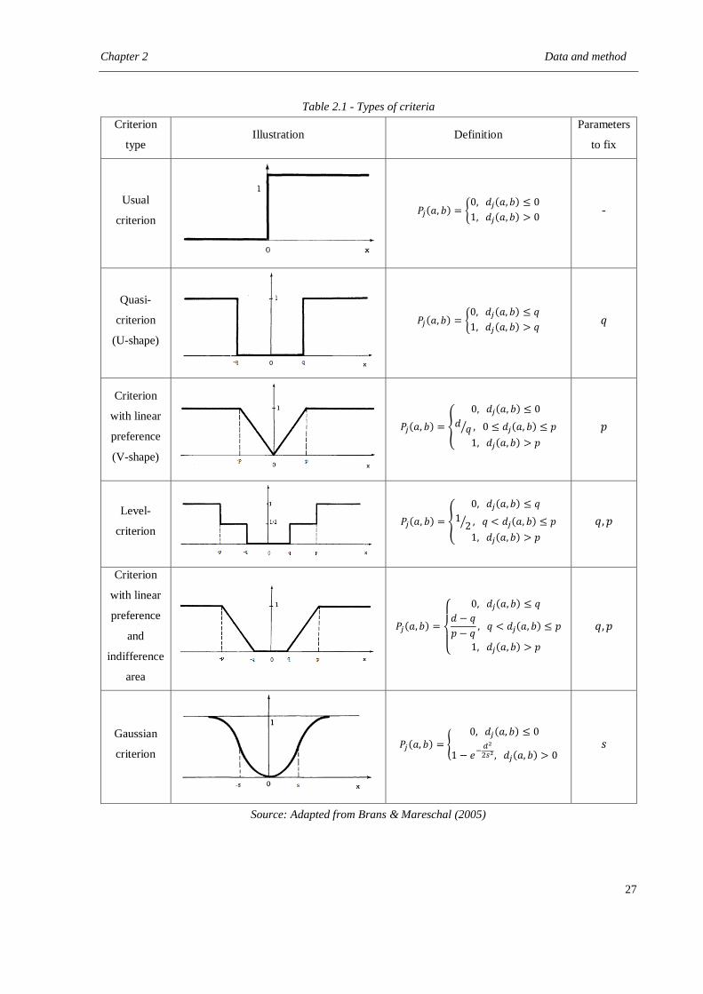
an alternative. The six types of criteria are shown in Table 2.1.
The six extensions require 0, 1 or 2 parameters. These parameters are the indifference
threshold (𝑞), preference threshold (𝑝) or 𝑠 (a value between 𝑞 and 𝑝). According to Brans &
Mareschal (2005), “The 𝑞 indifference threshold is the largest deviation which is considered as
negligible by the decision maker, while the 𝑝 preference threshold is the smallest deviation
which is considered as sufficient to generate a full preference.”. Brans & Vincke (1985) asserts
that the parameters have an economic significance, and then a decision maker should easily
understand them.
Other definition that needs to be made is the information between the criteria. The
decision maker needs to define a set of weights (𝑤𝑗 , 𝑗 = 1, 2,… , 𝑘) that means the relative
importance of each criterion. The higher the weight, more important is the criterion. It is
important to notice that ∑ 𝑤𝑗 = 1𝑘𝑗=1 .
Since the decision maker has the evaluation table, the weights, and the preference
function, the PROMETHEE method can be applied. Nowadays, many methods are available:
PROMETHEE I (partial ranking), II (complete ranking), III (ranking based on intervals), IV
(continuous case), V (segmentation constrains), VI (representation of the human brain), GDSS
(group decision), GAIA (visual interactive module), TRI (sorting problems), and CLUSTER
(nominal classification).
PROMETHEE methods have been applied in many contexts. According to Mareschal
(2016), 1390 papers were written about PROMETHEE since 1982 – one quarter of them are
related to methodology and the rest are applications. The majority of the studies are related to
Chapter 2 Data and method
27
Table 2.1 - Types of criteria
Criterion
type Illustration Definition
Parameters
to fix
Usual
criterion
𝑃𝑗(𝑎, 𝑏) = {0, 𝑑𝑗(𝑎, 𝑏) ≤ 0
1, 𝑑𝑗(𝑎, 𝑏) > 0 -
Quasi-
criterion
(U-shape)
𝑃𝑗(𝑎, 𝑏) = {0, 𝑑𝑗(𝑎, 𝑏) ≤ 𝑞
1, 𝑑𝑗(𝑎, 𝑏) > 𝑞 𝑞
Criterion
with linear
preference
(V-shape)
𝑃𝑗(𝑎, 𝑏) = {
0, 𝑑𝑗(𝑎, 𝑏) ≤ 0
𝑑𝑞⁄ , 0 ≤ 𝑑𝑗(𝑎, 𝑏) ≤ 𝑝
1, 𝑑𝑗(𝑎, 𝑏) > 𝑝
𝑝
Level-
criterion
𝑃𝑗(𝑎, 𝑏) = {
0, 𝑑𝑗(𝑎, 𝑏) ≤ 𝑞
12⁄ , 𝑞 < 𝑑𝑗(𝑎, 𝑏) ≤ 𝑝
1, 𝑑𝑗(𝑎, 𝑏) > 𝑝
𝑞, 𝑝
Criterion
with linear
preference
and
indifference
area
𝑃𝑗(𝑎, 𝑏) =
{
0, 𝑑𝑗(𝑎, 𝑏) ≤ 𝑞
𝑑 − 𝑞
𝑝 − 𝑞, 𝑞 < 𝑑𝑗(𝑎, 𝑏) ≤ 𝑝
1, 𝑑𝑗(𝑎, 𝑏) > 𝑝
𝑞, 𝑝
Gaussian
criterion
𝑃𝑗(𝑎, 𝑏) = {0, 𝑑𝑗(𝑎, 𝑏) ≤ 0
1 − 𝑒−𝑑2
2𝑠2 , 𝑑𝑗(𝑎, 𝑏) > 0 𝑠
Source: Adapted from Brans & Mareschal (2005)
Chapter 2 Data and method
28
environmental problems, services and/or public applications, and industrial applications.
Mareschal (2016) affirms that the large number of applied papers may be due to Visual
PROMETHEE software – a friendly and powerful tool. To know more about applications and
extensions of PROMETHEE methods, the literature review of Benzadian et al. (2010) should
be consulted – the authors say that the papers related to PROMETHEE has grown significantly.
We can mention some studies that were recently developed involving PROMETHEE
METHODS. Esmaelian et al. (2015) used PROMETHEE IV and geographical information
systems to solve emergency service station problems - they show a study case in the city of
Tehran. Banamar & Smet (2015) proposed an extension that considers temporal evaluations.
Smet & Sarrazin (2015) suggested another extension: they present an extension of
PROMETHEE I taking into account clustering problems. The work of Samanlioglu & Ayag
(2016) combined Analytic Network Process, PROMETHEE II and fuzzy logic to support
machine tool selection process. Fuzzy logic is also used by Lolli and colleagues (2016) – they
developed an approach to deal with waste treatment, considering traditional criteria of life cycle
assessments with social and economic criteria.
In this thesis, we opted to use PROMETHEE II; therefore, this method will be discussed
in details in the following subsection.
2.5.2.2 PROMETHEE II
As stated before, PROMETHEE II gives a complete ranking of the alternatives. Firstly,
we need to measure the preference between the alternatives, through pairwise comparisons. In
this sense, we need to measure the preference of alternative 𝑎 in relation to alternative 𝑏, and
the preference of 𝑏 in relation to 𝑎. This comparison should be made among all alternatives.
The preference will be measured by the preference index, according to Equation (2.6):
{𝜋(𝑎, 𝑏) = ∑ 𝑃𝑗(𝑎, 𝑏)𝑤𝑗
𝑘𝑗=1
𝜋(𝑏, 𝑎) = ∑ 𝑃𝑗(𝑏, 𝑎)𝑤𝑗𝑘𝑗=1
(2.6)
𝜋(𝑎, 𝑏) expresses how 𝑎 is preferred to 𝑏 over all criteria and 𝜋(𝑏, 𝑎) expresses how 𝑏 is
preferred to 𝑎 over all criteria. So, 𝜋(𝑎, 𝑏)~0 implies a weak global preference of 𝑎 over 𝑏, and
𝜋(𝑎, 𝑏)~1 implies a strong global preference of 𝑎 over 𝑏.
When all the preference indices are obtained, the outranking flows can be measured for
each alternative. The positive outranking flow (𝜙+) expresses how an alternative 𝑎 is
Chapter 2 Data and method
29
outranking all the others, while the negative outranking flow (𝜙−) expresses how an alternative
𝑎 is outranked by all the others. The outranking flows are calculated as Equations (2.7) and
(2.8), respectively:
𝜙+(𝑎) =1
𝑛−1∑ 𝜋(𝑎, 𝑥)𝑥∈𝐴 (2.7)
𝜙−(𝑎) =1
𝑛−1∑ 𝜋(𝑥, 𝑎)𝑥∈𝐴 (2.8)
Therefore, the positive outranking flow means power while the negative flow means
weakness of each alternative. The higher 𝜙+(𝑎) and the lower 𝜙−(𝑎), the better the alternative.
In order to build the complete ranking of PROMETHEE II, the net outranking flow also
needs to be calculated. Equation (2.9) gives the net outranking flow:
𝜙(𝑎) = 𝜙+(𝑎) − 𝜙−(𝑎) (2.9)
The net flow can range between -1 and 1: −1 ≤ 𝜙(𝑎) ≤ 1. The higher the net flow, the
better the alternative. According to the net flow of each alternative, it is possible to obtain a
total preorder (complete ranking without incomparability). The ranking can be obtained,
ordering the alternatives as Equation (2.10):
{𝑎 𝑜𝑢𝑡𝑟𝑎𝑛𝑘𝑠 𝑏 (𝑎𝑃𝑏) 𝑖𝑓𝑓 𝜙(𝑎) > 𝜙(𝑏)
𝑎 𝑖𝑠 𝑖𝑛𝑑𝑖𝑓𝑓𝑒𝑟𝑒𝑛𝑡 𝑡𝑜 𝑏 (𝑎𝐼𝑏) 𝑖𝑓𝑓 𝜙(𝑎) = 𝜙(𝑏) (2.10)
Therefore, through this methodology, all alternatives will be ranked, without
incomparability. Behzadian et al. (2010) summarize PROMETHEE II in five steps, as follow:
1. Determination of deviations based on pair-wise comparison
2. Application of the preference function
3. Calculation of an overall or global preference index
4. Calculation of outranking flows
5. Calculation of net outranking flow
2.5.3 Temporal analysis
The temporal analysis is aimed to answer two questions: (1) Is there temporal variation
in homicides in Recife taking into account seasons, months, days of week, and periods of day?;
Chapter 2 Data and method
30
and (2) Is there a difference between the spatial patterns of homicides when we consider
seasons, months, days of week, and periods of day?
The first question of this study, regarding the temporal variation of homicides, could be
answered in a simple and straightforward manner. Given that we wanted to investigate whether
the variation between the temporal units is statistically significant or not, the question could be
answered using ANOVA. With regard to the second question, we used the Spatial Point Pattern
Test developed by Andresen (2009) to check the spatial pattern of homicides. The software
Statistica was used to perform ANOVA while the graphical user interface developed by
Andresen and Malleson was used to run SPPT.
In order to develop the temporal analysis, the data were divided by seasons, months, days
of week, periods of day, weekday versus weekend, and day versus night. For the seasons, we
considered summer as the period between December and February, autumn as March to May,
winter as June to August, and spring as September to November. we divided the periods of day
as follows: 6am to 11:59am as morning, 12:00pm to 5:59pm as afternoon; 6pm to 11:59pm as
night; and 12:00am to 5:59am as dawn. It is important to note that we received the data from
SDS with these divisions, and we did not have access to the exact hour of the occurrences. In
the division of weekday versus weekend, we considered weekdays the days between and
including Monday and Friday, and weekends as Saturday and Sunday. Finally, regarding to the
division of day versus night, we considered the period between 6am to 5:59pm as day and 6pm
to 5:59am as night.
Regarding periods of day, few occurrences do not have this information, for unknown
reasons to the author. However, only 43 of the 8,446 homicides have missing data (0.51
percent). These homicides were considered in all analysis, except for periods of day and day
versus night. In addition, 20 occurrences (0.24 percent of all homicides) do not have geographic
coordinates, also for unknown reasons. Such occurrences were considered in the temporal
variation analysis (research question 1) but were not included on the spatial analysis (research
question 2). For the spatial analyses of different temporal units, we used census tracts as the
spatial units of analysis.
Chapter 2 Data and method
31
2.5.4 Spatial analysis
The purpose of the spatial analysis is to respond two questions: (1) Do homicides in
Recife follow the law of crime concentration at places? (2) If there is crime concentration in
Recife, are these spatial concentrations stable over time?
The methods necessary for answering the first research question were simple and
straightforward. Similar to the crime and place literature we calculated the percentage of areas
that have any homicides and the percentage of areas with any homicides that account for 50
percent of homicides.
In order to answer the second research question regarding the stability of the spatial
patterns of homicide in Recife, an analytical technique that can identify (statistically significant)
spatial change was necessary. The spatial point pattern test developed by Andresen (2009) has
the ability to identify the degree of similarity between two datasets. We checked the spatial
stability for years, seasons, months, days of week, periods of day, weekday versus weekend,
and day versus night.
For the spatial analysis, we used two units of analysis – census tracts and street segments.
However, we found a limitation in working with street segments. Georeferenced maps are
expensive and we only got a georeferenced map of the city of Recife. Therefore, homicide
concentration (research question 1) is the only analysis in this thesis that we will deal with the
city of Recife rather than Metropolitan Region of Recife. The analysis of the stability of spatial
patterns (research question 2), nevertheless, was made considering MRR.
2.5.5 Environmental analysis
This analysis has the objective of answer the following question: which environmental
factors are related to homicides in Recife? In this sense, we examined homicides and many
economic, social and demographic variables related to social disorganization theory. It is
important to say that we used census tracts as spatial unit and that all independent variables
were collected from 2010 demographic census.
The regression models were performed using R: The Project for Statistical Computing
(http://www.R-project.org) and the sphet package that allows for controlling heteroskedasticity
in a spatial regression context. The spatial error model was applied in this study because it
looked the most suitable for our data. Firstly, we tried linear regression but the Jarque-Bera and
Breusch-Pagan tests rejected their respective null hypotheses, indicating non-normality of the
Chapter 2 Data and method
32
errors and heteroskedasticity. Moreover, Lagrange Multiplier tests showed the presence of
spatial dependence of model residuals. Therefore, according to the results of Robust LM tests,
the spatial regression was chosen.
As such, our second set of analyses used the spatial error model available in sphet. This
software has the benefit of filtering out spatial autocorrelation and controlling for
heteroskedasticity through the use of robust standard errors. As such, all statistical inference
was based on heteroskedastic-consistent errors. The spatial error model filters out spatial
dependence that is present within the dependent and independent variables. The general
functional form of the spatial error model is as Equation (2.11):
𝑦 = 𝑋𝛽 + 𝜌𝑊𝜀 + 𝑢 (2.11)
where y is the number of homicides, Xβ is the matrix of independent variables and its
estimated parameters, W is the spatial weights matrix that captures the spatial association
between the different census units, ρ measures the strength of spatial association, is shorthand
for y – X, and u is the independent and identically distributed error term.
First order Queen’s contiguity was used to define the spatial weights matrices used in
the spatial regression analysis – this was sufficient to account for spatial dependence in all
regression models. The final model selection is based on a general-to-specific method,
considering all of the explanatory variables in the initial model, removing statistically
insignificant variables one at a time. In order to prevent the removal of statistically significant
variables that appeared insignificant because of multicollinearity, we also conducted sets of
joint significance tests (likelihood ratio tests); though important, these latter tests did not affect
the final regression model.
The number of homicides was used as dependent variable in this analysis, instead of
homicide rates; this has been identified as a better modeling strategy in neighborhood-level
spatial analyses of crime to control for population size because of issues relating to crime rate
calculations (Boivin, 2013). However, we also estimated count-data models to analyze which
model fits better to our data – Poisson and negative binomial models. Results indicated that the
spatial error model is a better fit, but the qualitative nature of the negative binomial results are
the same as spatial error model results.
Chapter 2 Data and method
33
2.5.6 Multicriteria analysis
The multicriteria analysis was performed to answer the following question: which are the
most vulnerable areas regarding to homicides? This question is important because some areas
need more attention from the government than others. Considering that it is not possible
preventing criminal occurrences in an entire city or neighborhood, some kind of priority needs
to be made. Therefore, it is important to identify the most critical areas in order to allocate
public resources to them.
We employed multicriteria approach to evaluate vulnerability, through PROMETHEE II
method. In order to measure the vulnerability of each census tract, we considered variables that
were pointed out as statistically significant in our environmental analysis. In this sense, we used
density, education, income, inequality, rented houses, and public illumination as determinant
factors of vulnerability to homicide.
The multicriteria approach was applied twice, first considering Metropolitan Region of
Recife and second considering the Boa Viagem neighborhood. Recife’s application gives us a
comprehensive view of the region. However, RMM is composed by more than 4,500 census
tracts and, because of that, the visualization of most critical areas is complex. In addition, it is
hard to make an analysis with such a large area. Due to this difficulty, we also identified the
most vulnerable areas considering a neighborhood, Boa Viagem. Working with a
neighborhood, allows a deeper analysis and even a preliminary proposal of actions to reduce
criminality.
2.5.6.1 Application in Metropolitan Region of Recife
This application took into account 4,494 census tracts of MRR. We applied
PROMETHEE II method for all census tracts, with the aid of Visual PROMETHEE Academic
Edition software. It is important to mention that it was a simulation, so we did not consult a
decision maker. PROMETHEE II offers as result the net flow for each area and this value can
be used to ranking the census tracts from the most vulnerable to the less vulnerable.
To map 4,494 census tracts according to its respective net flow is not instructive. Firstly,
because there are many areas to analyze and secondly because we are not considering the
surroundings. The surroundings are relevant here because a vulnerable area can affect its
neighbor (because of crime displacement, for example). In this sense, we opted to apply local
Moran’s I to evaluate the surroundings.
Chapter 2 Data and method
34
Anselin (1995) created the local Moran’s I as a local indicator of spatial association. This
indicator is able to measure the spatial association of an area with its surrounding; therefore, it
can identify clusters or outliers in a dataset. The local Moran’s I can be calculated as Equation
(2.12):
𝐼𝑖 =(𝑥𝑖−𝑥
∗)∑ 𝑤𝑖𝑗𝑗 (𝑥𝑗−𝑥∗)
∑ (𝑥𝑖−𝑥∗)2𝑖
𝑛⁄ (2.12)
where 𝑥𝑖 is the value of variable 𝑥 in spatial unit 𝑖, 𝑥∗ is the mean of 𝑥, 𝑛 is the number
of spatial units, and 𝑤𝑖𝑗 is the spatial weights matrix that measures the strength of the
relationship between two spatial units.
Local Moran’s I can be performed using ArcGIS 10.2 software, through Cluster and
Outlier Analysis tool. This tool is able to show four different types of spatial association: high-
high (HH) (area with high value surrounded by areas with high values – hot spots), low-low
(LL) (area with low value surrounded by areas with low values – cold spots), high-low (HL)
(area with high value surrounded by areas with low values – outlier), and low-high (LH) (area
with low value surrounded by areas with high values – outlier).
Therefore, the final result of this analysis is the map created by the Cluster and Outlier
Analysis tool, taking into account the net flow of PROMETHEE II. However, this result still is
complicated to be discussed due to the magnitude of the area. Because of that, another
application was made in a smaller area: Boa Viagem neighborhood.
We used Visual PROMETHEE Academic Edition, ArcGIS 10.2, Google Street View,
and Google Earth to perform this application.
2.5.6.2 Application in Boa Viagem neighborhood
Boa Viagem is a neighborhood of the city of Recife composed by 168 census tracts. The
vulnerability regarding homicides was also evaluated for this area, using PROMETHEE II.
However, three different approaches were tested:
a. PROMETHEE II method was applied for all 168 census tracts and a ranking was
created considering the net flow.
b. We grouped the census tracts by similarity through Grouping Analysis tool from
ArcGIS. After, we applied PROMETHEE II on these groups and ranking them
considering the net flow.
Chapter 2 Data and method
35
c. PROMETHEE II method was applied for all 168 census tracts and local Moran’s
I was performed to identify clusters and outliers (according to net flow).
These three approaches showed a similar result, but we decided to deal with option (b).
A more detailed discussion about the three options and its advantages and disadvantages is
made in Chapter 9. Option (b) was not viable for Recife because there are many census tracts
and then the grouping would be complicated.
We used Visual PROMETHEE Academic Edition and ArcGIS 10.2 to perform this
application. We also utilized Google Street View and Google Earth to obtain images from the
vulnerable areas.
2.6 Final comments
This chapter was aimed to discuss about the data and the methodology of this thesis. Our
study was concentrated in the Metropolitan Region of Recife and the Boa Viagem
neighborhood. We used data from the Secretariat of Social Defense and DATASUS (provided
by Ministry of Health). We also used data from the demographic census of 2010, provided by
the Brazilian Institute of Geography and Statistics. In our analyses, we employed two spatial
units: census tracts and street segments.
This thesis involves five different analyses. The first one is a temporal analysis, with the
objective of investigate temporal variations of homicides in Recife. In this sense, we used
ANOVA and SPPT. In the second analysis, we developed a spatial study, in order to verify the
stability or not of homicides. Again, SPPT was considered. In the third analysis, we made an
environmental study, with the intent of discover social, economic, and demographic factors
related to homicide. For this analysis, we applied spatial regression. In the last two analyses,
we performed a preliminary attempt to identify the most vulnerable areas of homicides in the
Metropolitan Region of Recife and the Boa Viagem neighborhood. We used PROMETHEE II
multicriteria method, local Moran’s I, and cluster analysis.
Chapter 3 Theoretical background and literature review
36
3 THEORETICAL BACKGROUND AND LITERATURE REVIEW
This chapter has the objective of present two theories that can explain the phenomenon
of crime and present research that has been written specifically about homicides. There are
many theories able to describe criminal behavior as a whole; however, we chose to detail two
theories because our findings suggest that they can explain homicide in Recife. Therefore, in
this chapter we will discuss social disorganization theory and routine activity theory. In
addition, this chapter offers a literature review specific for homicides, the main concern of this
study. In sections 3.2 to 3.4, we show research regarding homicide and temporal variation,
homicide and spatial analysis, and homicide and environmental factors, respectively –
presenting research developed globally and specifically in Brazil.
3.1 Theories about crime
In this section, we will discuss only two theories regarding criminal behavior: social
disorganization theory and routine activity theory We are aware that there are many theories
able to explain the violent behavior – Deterrence Theory, Rational Choice Theory, Crime
Opportunity Theory, Social Learning Theory, Social Strain Theory, Social Bonding Theory,
Biosocial Theories, and so on. However, our findings showed that the first two theories are
satisfactory to explain the occurrence of homicides in Recife; therefore, they will be discussed
in details. Moreover, the investigation of other theories involves different factors that are out of
the scope of this thesis (and further, it requires additional data).
3.1.1 Social disorganization theory
One of the most common theoretical frameworks used to understand the spatial
distribution of crime, including homicide, is social disorganization theory. Though spatial, or
ecological, studies of crime date back to the early 1800s in France (Quetelet, 1842), social
disorganization theory and its focus on smaller units of analysis, such as neighborhoods, has its
roots in the Chicago School of sociology from the early twentieth century (Shaw et al., 1929;
Shaw & McKay, 1931, 1942).
In this framework, the level of social organization in an area is directly linked to the level
of criminal activity: less social organization leads to more crime. This is simply because without
social organization a neighborhood cannot come together or organize to prevent criminal
activity. The two primary drivers of a lack or social organization during this time were ethnic
Chapter 3 Theoretical background and literature review
37
heterogeneity and population turnover. Regarding ethnic heterogeneity, the neighborhood
residents literally could not speak to one another to discuss common issues. With population
turnover, very few residents would be willing to invest the time to discuss common issues
because they planned to leave the neighborhood as soon as possible. In both cases, social
disorganization emerges, as does the corresponding crime. In their own research, Shaw &
McKay (1942) found strong support for their theoretical framework.
Therefore, we can say that this theory is closely related to the neighborhood and puts forth
that the criminal behavior is strongly affected by the person's residential location. Social
disorganization theory also asserts that neighborhood characteristics are more significant than
individual characteristics. However, the theory is very misunderstood because people try to
understand social disorganization theory reading new papers, ignoring the original works. For
example, many people think that economic condition has a direct causal with crime rates but
the theory does not affirm that.
There have been two tests of social disorganization theory by contemporary researchers
that are significant. The first test of social disorganization theory that considered community
organization used the British Crime Survey. This research was undertaken by Sampson &
Groves (1989) who extended the concepts of Shaw & McKay (1942) to include sparse local
friendship networks, unsupervised teenage peer groups, and low organizational (neighborhood)
participation. In their causal model, Sampson & Groves (1989) found strong support for social
disorganization theory. This support for social disorganization theory was critical because
through the British Crime Survey these researchers were able to directly measure aspects of
social disorganization theory. And, equally important, they were able to show that social
disorganization theory was still relevant 60 years later.
The second test of social disorganization theory revisited the work of Sampson & Groves
(1989), considering subsequent iterations of the British Crime Survey (Lowenkamp et al.,
2003). This subsequent research confirmed the results of Sampson & Groves (1989), further
showing the relevance of social disorganization theory in a more recent context.
The difficulty with social disorganization theory, however, is operationalizing the
primary factors that have a causal link to criminal activity: sparse local friendship networks,
unsupervised teenage peer groups, and low organizational (neighborhood) participation. Such
information is available through some of the more comprehensive crime victimization surveys,
but is far from universal. This is why there are so few direct tests of social disorganization in
Chapter 3 Theoretical background and literature review
38
the literature. However, as outlined in the causal model of Sampson & Groves (1989), these
three primary factors are influenced by low economic status, ethnic heterogeneity, residential
mobility, family disruption, and urbanization. These latter factors influence the primary factors
that then affect criminal activity.
In the spatial criminology literature, in particular those studies that employ census-based
variables, research that considers social disorganization theory uses these latter factors to
represent the primary factors of social disorganization theory. Ethnic heterogeneity represents
the ability of residents to form friendship networks because of language and cultural barriers.
Low economic status represents the willingness to engage in organizational participation, for
example. The research in this area has used census-based variables such as the percentage of
recent immigrants, direct measures of ethnic heterogeneity, the unemployment rate, the
percentage of people with a university degree, average family income, the standard deviation
of average family income, the percentage of single-parent families, and the percentage of rental
residences in the spatial unit (see Andresen, 2006; Cahill & Mulligan 2003; Linsky & Straus
1986; Stark 1996; Tseloni et al. 2002).
3.1.2 Routine activity theory
Routine activity theory has a significant difference from social disorganization theory:
while social disorganization theory takes into account the neighborhood characteristics, routine
activity theory is concerned about individuals and specific points in space and time. Therefore,
routine activity theory is related to people making choices in space and time, not to
neighborhood characteristics affecting people.
For Cohen & Felson (1979), routine activities are “any recurrent and prevalent activities
which provide for basic population and individual needs, whatever their biological or cultural
origins”. According to Andresen (2014), “routine activities most often occur at the same or
similar times each day (rhythm), we can measure their frequency rate (time), and these activities
involve the coordination of multiple persons moving through societal space (timing)”.
Cohen & Felson assert that crime occurs when three factors are present at the same time
and in the same space: a motivated offender, a suitable target (person or thing), and the lack of
a capable guardian – somebody/something to prevent the crime from occurring. The lack of
anyone of these three elements will prevent criminal events. The convergence of these three
Chapter 3 Theoretical background and literature review
39
factors is totally related to routine activities: routine activities determine where and when
offenders, victims, and guardians will be.
However, we have to notice that routine activity theory is not a general theory of crime.
Due to the contact between offender and victim, this theory is not useful to explain crimes in
which this convergence does not exist – like cybernetic and white-collar crimes, for example.
Routine activity theory explains the sociological paradox in two ways. After the Second
World War, the economic condition increased such that people were able to spend their money
on leisure activities to go shopping, eat out, watch movies, and so on. In addition, after the War,
many cultural and social behaviors changed – for example, young people left home and women
started to work. Therefore, all these changes can explain the crime rise because more people
were outside of the relatively protective environment of the home (and consequently increasing
the chances of be a victim). Moreover, the increase of crimes can be understood through the
accessibility of the goods. More people are going out with their goods and this increases the
number of suitable targets. Furthermore, the goods have become much easier to steal, because
they are lighter and smaller.
The work of Cohen & Felson (1979) also provided empirical support for their theory.
They used criminological data and unexpected resources like Sears Catalog and Costume
Reports magazine. According to Andresen (2014), some of the findings were: people living in
single-adult households and those who worked outside the home had higher rates of direct-
contact predatory criminal victimization; adolescents, young adults, and non-married persons
had higher rates of direct-contact predatory criminal victimization; the rate of out-of-town travel
and the number of vacations taken by Americans created more opportunities for residential
burglary; changes in household activity (increases in the time spent away from the relatively
protective environment of the home) was positively associated with all crime types. Therefore,
the findings were supportive of routine activity theory and there are other works evaluating this
theory.
3.2 Homicide and temporal variation
There are many studies analyzing temporal variations of crime. These works, however,
do not achieve a common conclusion, mainly about the seasonality of homicides. In this
context, this section aims to present some papers regarding temporal changes in homicide –
considering all world and Brazil, specifically.
Chapter 3 Theoretical background and literature review
40
3.2.1 Previous research on temporal variations of homicide
There is a large volume of research investigating crime and temporal/climate variations,
particularly in the United States. However, there is not a lot of research that has found seasonal
variations in homicide. Anderson (1987) compared temperature and seven crime types with
data from the United States. His findings showed that the period between April and September
is the most violent. This period has the longest days, vacations, concentration of outdoor
activities, and higher alcohol consumption. Because of these characteristics, Anderson (1987)
concluded that the seasonal crime variation is more related to peoples’ activities and not a
consequence of temperature. In an investigation of homicide seasonality in Finland, Tiihonen
and colleagues (1997) found that the frequency of homicides during the winter was lower than
the expected (6 percent) and during the summer was higher (6 percent). These results, therefore,
revealed a seasonal component of homicides in Finland, but not to the same degree as found
with assault in other contexts – see Harries et al. (1984).
Other works, however, did not find evidence for the seasonality of homicides: Block
(1984) did not find seasonal fluctuations in United States and Canada, Abel et al. (1985) in
New York, Cheatwood (1988) in Baltimore, and Landau & Fridman (1993) in Israel. Yan
(2000) analyzed homicides in Hong Kong, also not finding evidence for seasonality, or any
significant relationships with climate variables. Finally, according to Rock et al. (2008), there
was no seasonality of homicides in England and Wales, but there was seasonality for assault.
In relation to the most violent months regarding homicides, the literature also presents
mixed results. The studies of Abel et al. (1985) and Cheatwood (1988), for example, did not
find monthly variation of homicides in New York and Baltimore. However, other works found
greater incidence of homicides in specific months, normally summer months and months that
typically have high levels of social interaction. Falk (1952) used data from eight American
cities and found that the most violent month is July (summer). Lester (1979) found a similar
result, also for United States: July and December. Tennenbaum & Fink (1994), considering the
United States, found that July and August (summer) have more homicides. McDowall et al.
(2012) analyzed 88 cities in United States and found a peak of homicides in August (summer).
In Israel, Landau & Fridman (1993) found August to be the most violent month. Moreover, in
Finland, Tiihonen et al. (1997) pointed out that the months with more occurrences of homicides
are July and August, while the months with fewer homicides are January and February.
Chapter 3 Theoretical background and literature review
41
However, despite the mixed results for more aggregated temporal analyses (seasons and
months), far more consistency in results emerge in the research that considers particular days
of the week. Specifically, there is a greater incidence of homicides during weekends. For
example, Saturdays and Sundays were pointed out as most violent days (considering homicides)
by Falk (1952), Lester (1979), and Abel et al. (1985). Regarding the other days, Falk (1952)
found high incidence on Mondays while Abel et al. (1985) found the opposite – Mondays are
the days with fewer homicides. Greenberg & Schneider (1992) also found that homicides are
more frequent on weekends, primarily for Caucasians. However, among African-American
young males, the frequency was found to be greater on Thursdays. Additionally, Lester (1979)
concluded that there was also an increase of homicides during national holidays. Finally, Lester
& Frank (1988) investigated whether homicides were more frequent on the first days of the
month, a phenomenon of suicides, but they did not find evidence for this hypothesis.
This brief summary of the literature clearly shows that there is little consensus regarding
the seasonality of homicides. Some authors suggest some reasons for this lack of consensus.
Tennenbaum & Fink (1994) assert that the seasonality effect is not easily detected because the
seasonal influences are small within any given year. Therefore, according these authors, data
with a longer time span using the appropriate statistical tools would be necessary to capture this
effect. Longer study periods are considered in the works of Tiihonen et al. (1997) and
McDowall et al. (2012). McDowall et al. (2012) state that is not appropriate to aggregate
different areas because the seasonal effect can be different in each location. Consequently, any
aggregation can change the results. Lastly, the study by Cheatwood (1988) identifies four
reasons for the difference between the findings: distinct data, definitions, or methods; regional
differences; urban / rural differences; and a lack of clarity on the questions that are been made.
3.2.2 Previous research on temporal variation of homicide in Brazil
Studies that analyze criminal occurrences with temporal/climatic variables are not
common in a Brazilian context. We only found one work that was published in an international
journal (Ceccato, 2005). However, we were able to identify a number of monographs, theses,
books, and articles from Brazilian journals (all of them were written in Portuguese). Generally
speaking, this research has shown that crimes are more common during summer, weekends,
and evenings.
Chapter 3 Theoretical background and literature review
42
Ceccato (2005) analyzed homicides in the city of São Paulo between 2000 and 2002. She
found that homicides are less frequent during winter, almost three fewer homicides per day.
According to her findings, weekends (54 percent of homicides) and the period between 8pm
and 2am (44 percent) are most dangerous. The conclusions of Maia (1999) and Bando (2012)
are in line with the findings of Ceccato (2005). Maia (1999) analyzed homicides in the state of
São Paulo and found Saturdays and Sundays to be the most frequent days for homicide. Maia
(1999) also found that there is not a high monthly variation, but January, March, and April
presented a notable increase in relation to the rest of the year. Bando (2012) also studied São
Paulo city and found a high concentration of homicides during weekends. His findings
identified summer as the season with the most occurrences, highlighting the months of January
and February. Bando (2012) also investigated homicides during important dates in Brazil: he
found that homicide peaks during Christmas and New Year, but decreases during carnival.
In Pernambuco, Oliveira Júnior (2013) found a greater volume of homicides in December
and January. He studied 30 years of data (1981 to 2010), considering homicides for both
genders with victims between 20 and 59 years old. According to Britto & Ferreira (2013), the
book by Francisco de Assis Mendonça (Clima e Criminalidade – Climate and Criminality)
asserts that December is the month with the most homicide occurrences in Recife, with winter
months having fewer occurrences. Moreover, in the city of Petrolina (Pernambuco State),
Campos and colleagues (2011) found that January, October, and December are the most violent
months. These authors also found that almost half of homicides occur during weekends, as well
as almost half of homicides occur between 6pm and 12am.
With regard to Minas Gerais State, Beato Filho et al. (2000) analyzed violent crimes that
occurred between 1991 and 1997. They found seasonal variations in homicide and rape, with
more crimes occurring between January to March and October to December. Britto & Ferreira
(2013) studied homicides in the city of Juiz de Fora (Minas Gerais State) from 1980 to 2012,
and compared these violent crimes with climatic variables. They found September and February
to be the most violent months and that homicide is related to temperature and rain. However,
they affirm that these results come from 30 years aggregated data and are related to a monthly
analysis. Finally, the work of Silva (2001) explores the temporal variation of homicides in Belo
Horizonte (Minas Gerais State), from 1995 to 2000. He found that homicides are more frequent
during weekends, when the rates are almost two times greater than weekdays. Regarding the
time of day, Silva (2001) found that the peak of homicides is between 7pm and 2am.
Chapter 3 Theoretical background and literature review
43
As can be seen from this review, Brazilian studies also present mixed results in relation
to the temporal variation of homicide (seasons and months). The reasons pointed out in the
previous subsection can explain the differences among Brazilian findings (aggregation of
regions, different time span, and different methods, for example). Moreover, the results may be
mixed because the cities can have different climates – Brazil is a geographically large country.
Regardless of these mixed results, there is far greater consistency in the research (Brazilian and
otherwise) when considering finer temporal scale of analysis: days of week and period of day.
Consequently, any investigation of temporal variations in homicide should consider more than
just one temporal scale to understand this phenomenon.
3.3 Homicide and space
According to Brantingham & Brantingham (2008), crime follows patterns, as well as the
decisions to commit a crime and the process of committing crime. The phenomenon of crime
is not random in time and space. Due to this relative predictability of crime, is possible to study
these patterns in order to understand and/or prevent criminal events.
Some of the research over the past 25 years within spatial criminology has shown that
crime is highly concentrated in a small number of places (Curman et al., 2015; Sherman et al.,
1989; Weisburd & Amram, 2014). Importantly, these places are referred to as micro-spatial
units of analysis, such as street segments and intersections or actual addresses. This relatively
small literature has been able to replicate this finding in a number of cities across the United
States, Canada, and Israel. Because of the consistency of these results, David Weisburd and
colleagues (2012) have put forth the “law of crime concentration at places”. They recognize the
presence of chronic street segments in parallel with the long-known fact that a few chronic
offenders commit the vast majority of crimes (Wolfgang et al., 1972), along the lines of the
Pareto principle.
The first study to emerge in this literature considering an entire city was that of Sherman
and colleagues (1989) who investigated robbery, motor vehicle theft, and rape in Minneapolis,
Minnesota. These researchers found that 3 percent of street segments in Minneapolis accounted
for 50 percent of these crimes: 2.2 percent for robbery, 2.7 percent of motor vehicle thefts, and
1.2 percent for rape. In a similar study on Seattle, Washington, Weisburd and colleagues (2004)
found that 5 percent of Seattle’s street segments accounted for 50 percent of police calls for
service over a 14-year period. Weisburd and colleagues (2012) replicated this over a 16-year
Chapter 3 Theoretical background and literature review
44
period as well as in the context of juvenile offending (Weisburd et al., 2009). Also in the United
States, Braga and colleagues (2010; 2011) found similar percentages in the contexts of gun
violence and commercial street robberies in Boston, Massachusetts.
In a Canadian context, Andresen & Malleson (2011) and Andresen & Linning (2012)
found similar results for Vancouver, British Columbia and Ottawa, Ontario, respectively.
Specifically, analyzing assault, burglary, robbery, sexual assault, theft, theft of vehicle, and
theft from vehicle in Vancouver, Andresen & Malleson (2011) found that 50 percent of the
police calls for service for these crimes were accounted for 1 to 6 percent of street segments,
most often less than 3 percent of street segments. In Ottawa, analyzing burglary (commercial
and residential), robbery (commercial, individual, and other), and theft of vehicle, Andresen &
Linning (2012) found that 50 percent of these crime occurred in less than 1.7 percent of street
segments. Most recently, Weisburd & Amram (2014) found that 4.5 percent of street segments
accounted for all criminal incidents in Tel Aviv-Jaffa, Israel.
Not only has the crime and place literature generated a number of interesting facts
regarding the spatial concentrations of crime, there have been a number of interesting
theoretical and practical applications of these works. For example, researchers have argued that
we need to consider the micro-place when understanding theory. In the context of routine
activity theory, motivated offenders and suitable targets converge in time and space (with the
lack of a capable guardian) in order for a criminal event to occur (Cohen & Felson, 1979).
However, though this convergence technically occurs within a neighborhood, it really occurs
at a discrete location. Knowing why the convergence occurred at one street segment and not
the one next to it could prove to be of theoretical importance (Andresen & Malleson, 2011;
Groff et al., 2010).
Weisburd et al. (2012) have undertaken some interesting analyses in the context of social
disorganization theory, finding significant variability of social disorganization theory variables
within larger geographic units. In the context of practical applications, crime prevention,
Sherman et al. (1989) note how it is easier to change the routine activities of places than people.
Of course, these researchers were speaking of how people used these places for their routine
activities, but this highlights the importance of understanding the places at which crime
concentrations occur.
In relation to crime decreases, there are two studies in the literature that have investigated
the patterns of crime decreases: Weisburd and colleagues (2004), in Seattle (Washington); and
Chapter 3 Theoretical background and literature review
45
Curman et al. (2015), in Vancouver (British Columbia). Weisburd and colleagues have also
undertaken some extensions of this work and Braga et al. (2010; 2011) have used another
method (growth curve analysis) with similar results. Both of these studies reported a decrease
in crime at the level of the city (24 and 40 percent, respectively). Most interesting is that even
though the overall crime patterns at places were stable over time, the crime drops in each of
these cities could be explained only considering a small percentage of street segments. In
Vancouver, all street segments were stable or decreasing over time, but in Seattle some street
segments were increasing in their levels of crime.
However, studies regarding homicide and place are scare in the literature. As homicide is
a rare event, any spatial analysis is a challenge due to the small number of occurrences.
Therefore, it is a hard task to find in the literature studies concerning spatial analysis of
homicides. Sometimes, some researchers involve homicide in their analysis considering violent
crime; however, homicides are inexpressive within this group.
3.4 Homicide and environmental factors
In the literature, we can find many studies relating environmental factors and crime. These
works normally compare crimes with social, economic, and demographic variables. The
empirical method to analyze the relation among crime and these factors is not a common point,
as well as the findings are frequently different. Sometimes, opposite relationships are found for
the same variable; however, the context where the study is made needs to be taken into account.
This section aims to show papers that were written in this area, considering both global research
and research in Brazil.
3.4.1 Recent research on homicide and environmental factors
Many works analyzing homicide (or violent crimes) and census variables can be found.
Below, we show the findings of some of these studies applied in all world.
Blau & Blau (1982) realized a research involving 125 metropolitan regions of United
States and considering occurrences of 1970. As dependent variables, they used crime rates of
four violent crimes, including homicide. The independent variables were population size,
percent black, percent poor, geographical region, income inequality, percent divorced, and
racial socioeconomic inequality. They employed a regression analysis based on ordinary least
squares. The findings suggest that violent crimes increase due to socioeconomic inequality
between races and economic inequality generally.
Chapter 3 Theoretical background and literature review
46
In Germany, Entorf & Spengler (2000) analyzed socioeconomic and demographic factors.
These authors made their study based on the Becker-Ehrlich deterrence model and examined
crimes from 1975 to 1996. They considered as explanatory variables: foreign citizens, income
per capita, unemployment rate, unemployment among youths, and males aged 15-24.
According to the results, Entorf & Spengler (2000) asserts that income variables are able to
better explain property crime than violent crime. Therefore, the deterrence hypothesis was
confirmed for property crimes.
In his work, Kelly (2000) analyzed the relationship between inequality and violent and
property crimes. He found that inequality has a significant influence on violent crimes but not
for property crimes. In addition, he considered variables involving poverty, education, race, and
intensity of police activity. This study concluded that violent crimes are significantly influenced
by the proportion of female headed families, population mobility, proportion of young people,
and inequality. Police activity or poverty do not impact violent crimes strongly. The data is
related to United States, year 1991.
A study was undertaken in the city of Camden, New Jersey, by Gorman and colleagues
(2001). They considered variables regarding the social structure of the neighborhood, alcohol
outlet density, and violence. Bivariate analyses showed significant and positive relations of
violent crime with proportion population aged 12-17 years, welfare rate, and alcohol outlet
density. On the other hand, the results showed a negative relationship with population turnover
and proportion of elderly population. However, the spatial regression only confirmed the
significance with population turnover, proportion population aged 12-17 years, welfare rate,
and alcohol outlet density.
Fajnzylber and colleagues (2002) studied the determinants of homicide and robbery for
79 countries (45 for homicide and 34 for robbery), for the period 1970-1994. The countries
include Western Europe, United States, Canada, Japan, etc. They used variables related to
income, inequality, education, deterrence, drugs, urbanization, and young males. Generalized
method of moments (GMM) methodology was used to analyze this problem and the results
indicate that homicide has a negative relation with GDP growth rate and a positive relation with
Gini index.
The study of Buonanno & Montolio (2008) analyzed total crimes, crimes against
property, and crimes against person in 46 Spanish provinces. They used data from 1993 to 1999
and applying ordinary least squares regression and the GMM-system estimator. The
Chapter 3 Theoretical background and literature review
47
explanatory variables were separated into three groups: deterrence variables, demographic
variables, and socio-economic variables. Initially, the ordinary least squares showed
statistically significance with foreigners, urbanization, males aged 25-29, education, per capita
income, and condemn. Among these variables we can highlight the percentage of young males
(biggest coefficient: 0.2785). However, the GMM-system estimator only revealed urbanization
as significant.
Haddad & Moghadam (2010) compared crimes against person and property with
deterrent, social, economic, and demographic factors. The authors used data from the provinces
of Iran for the period 1997-2005. The results show that deterrence factors, unemployment, and
migration are not significant with violent crimes. However, the analysis reveals statistically
significance with family average income, divorce rate, population density, and literacy rate.
Moreover, literacy presents a strong negative impact in violent crimes.
Altindag (2012) used data from 33 countries of Europe, regarding the years 1995 to 2003.
According to ordinary least squares regression, he found only two statistically significant
variables: police rate and percentage of urban population. The objective of this work was
analyzing the relation between crime rates and unemployment; however, the regression did not
show a significant relation with homicide. For property crimes, the relation with unemployment
was very strong, with a coefficient of 43.10 and significant at 1 percent.
Lee et al. (2014) performed an analysis to discover if there is advantage in aggregating
homicide and suicide. Besides that, the authors made multivariate analysis considering
inequality and unemployment. The regression model revealed statistically significant relation
(positive) between homicide and unemployment. They used data from 40 countries (nations in
the World Health Organization with available data) for the years 1962-2008.
The works mentioned above show many factors pointed out as determinants of
criminality. It is important to notice that each finding will depend on the context of study.
However, we can observe that there is something in common among the results: they are in a
certain way related to social disorganization theory. Finally, we want to mention that this review
about the determinants of crime is not exhaustive.
3.4.2 Recent research on homicide and environmental factors in Brazil
Barata & Ribeiro (2000) analyzed homicides occurred in 1996 in the municipalities of
São Paulo. The main objective of this research was to investigate the relation between homicide
Chapter 3 Theoretical background and literature review
48
and income inequality. They did not found a strong relation between the Gini index and
homicide, but they found a positive relationship when the size of population was controlled for.
The findings suggest that as long as the population and the income of household heads increase,
income inequality is a significant factor for homicides.
Gawryszewski & Costa (2005) analyzed homicide rates for the year 2000 across the 96
administrative units in São Paulo City. These authors considered the infant mortality rate,
average income, proportion of adolescent mothers, population density, and the percentage of
children not attending school. Using a bivariate correlation analysis, Gawryszewski & Costa
(2005) found that the homicide rate was positively related to the infant mortality rate, the
percentage of adolescent mothers, and the percentage of children not attending school, whereas
the homicide rate was negatively associated with average income – population density had a
positive but statistically insignificant relationship with homicide rate. However, in a regression
context, only the percentage of children not attending school and monthly average income
remained statistically significant.
In a spatial analysis of homicide in the districts of the State of Pernambuco, Lima et al.
(2005b) analyzed homicide rates considering an index of living conditions, a human
development index, per capita family income, the Theil index, the Gini index, the average
income of the head of the family, a poverty index, a rate of illiteracy, and population density.
Homicide rates were statistically related to all of these independent variables in a correlation
analysis, only with the illiteracy rate and poverty index being retained in the final regression
models as statistically significant. In a linear regression model, these two variables were able
to account for almost 25 percent of the variation in the homicide rate.
Sachsida et al. (2007) analyzed homicide rates across Brazilian states, 1981 - 1995,
considering average family income, law enforcement spending, urbanization, the Gini index,
the unemployment rate, schooling, and poverty. These authors undertook a variety of regression
models (ordinary least squares, random effects, and fixed effects) and found that income
inequality, urbanization, and unemployment were all statistically significant and positively
related to state level homicide rates.
Ceccato et al. (2007) analyzed homicide in São Paulo, Brazil using police districts,
standardized homicide ratios, low income, the presence of slum areas, alcohol problems, urban
areas, the presence of transportation nodes, the presence of bars and restaurants, and betting
Chapter 3 Theoretical background and literature review
49
houses. Ceccato and colleagues found that homicide was strongly related to low-income, the
presence of transportation nodes, the availability of weapons, and drug-related activity.
Araújo et al. (2010) found that ethnicity played a statistically significant role in the
prediction of homicide in Salvador, Brazil. Specifically, Araújo et al. (2010) found a positive
relationship between the presence of black males aged 15 to 49 and homicide rates. They
explain that this result emerges from a long history and process of social inequality in Brazil.
As noted by Kilsztajn et al. (2003), there is an overrepresentation of this population who are
poor and male; as such, any inference with regard to such a variable must be made with caution.
Battela & Diniz (2010) used Pearson correlation to evaluate the determinants of
criminality in Minas Gerais State. These authors tested 21 variables that are divided in seven
classes: human development, wealth, inequality, infrastructure, education, structure of
population, and immigration. Regarding violent crimes against person, they found that human
development, infrastructure, and education have a negative relationship while wealth,
inequality, structure of population, and immigration have positive relation.
The work of Peres et al. (2011) went beyond environmental variables and explored the
investment in social policies and public security. They performed Spearman correlations
between the variation of homicide rate and 11 variables. The findings showed a statistically
significant correlation (positive) with young population, unemployment, investment in policies
of education and culture, municipal investment in public security, and rate of seized arms.
Resende & Andrade (2011) examined data from all Brazil (municipalities with more than
100,000 inhabitants) about different crime types (data of 2004). They collected homicide data
from two sources, DATASUS and SENASP. For both datasets they found statistically
significance with Gini index (positive), police actions (negative), and access of television
(positive). However, for SENASP dataset they also found a positive relationship with poverty.
Most recently, but in an analysis that pools Brazil with other countries that have high
homicide rates, Loureiro & Silva (2012) investigated homicide considering life expectancy, the
Gini index, economic growth, the human development index, and the rate of urbanization.
Similar to the research that focuses on Brazil, Loureiro & Silva (2012) found that income
inequality, low human development, and low life expectancy were all associated with higher
levels of homicide.
Finally, Menezes et al. (2013) used linear and spatial regression to analyze homicides in
Recife (2008 to 2010). They considered inequality, socioeconomic, and environmental
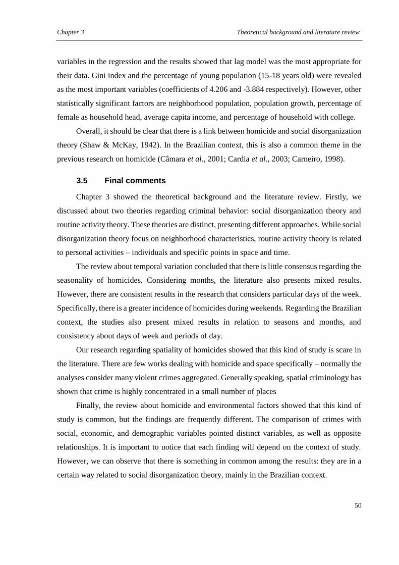
Chapter 3 Theoretical background and literature review
50
variables in the regression and the results showed that lag model was the most appropriate for
their data. Gini index and the percentage of young population (15-18 years old) were revealed
as the most important variables (coefficients of 4.206 and -3.884 respectively). However, other
statistically significant factors are neighborhood population, population growth, percentage of
female as household head, average capita income, and percentage of household with college.
Overall, it should be clear that there is a link between homicide and social disorganization
theory (Shaw & McKay, 1942). In the Brazilian context, this is also a common theme in the
previous research on homicide (Câmara et al., 2001; Cardia et al., 2003; Carneiro, 1998).
3.5 Final comments
Chapter 3 showed the theoretical background and the literature review. Firstly, we
discussed about two theories regarding criminal behavior: social disorganization theory and
routine activity theory. These theories are distinct, presenting different approaches. While social
disorganization theory focus on neighborhood characteristics, routine activity theory is related
to personal activities – individuals and specific points in space and time.
The review about temporal variation concluded that there is little consensus regarding the
seasonality of homicides. Considering months, the literature also presents mixed results.
However, there are consistent results in the research that considers particular days of the week.
Specifically, there is a greater incidence of homicides during weekends. Regarding the Brazilian
context, the studies also present mixed results in relation to seasons and months, and
consistency about days of week and periods of day.
Our research regarding spatiality of homicides showed that this kind of study is scare in
the literature. There are few works dealing with homicide and space specifically – normally the
analyses consider many violent crimes aggregated. Generally speaking, spatial criminology has
shown that crime is highly concentrated in a small number of places
Finally, the review about homicide and environmental factors showed that this kind of
study is common, but the findings are frequently different. The comparison of crimes with
social, economic, and demographic variables pointed distinct variables, as well as opposite
relationships. It is important to notice that each finding will depend on the context of study.
However, we can observe that there is something in common among the results: they are in a
certain way related to social disorganization theory, mainly in the Brazilian context.
Chapter 4 Homicide in Brazil, Pernambuco, and Recife
51
4 HOMICIDE IN BRAZIL, PERNAMBUCO, AND RECIFE
Before starting the detailed analyses of homicides in Recife, it is important to present the
scenario of Brazil, Pernambuco, and Recife with regard to this crime type. In this way, this
chapter has the aim of showing homicide numbers and reveals some peculiarities of this
phenomenon in these places. Moreover, in the last section we present a program employed in
the State of Pernambuco concerned on reducing violent deaths: Pact for Life.
4.1 Homicide in Brazil
In the introduction of this thesis we mentioned some facts about Brazil that must be cited
again: (1) Brazil has a higher homicide rate than the most populous countries in the world; (2)
10 percent of homicides in the world in 2012 occurred in Brazil, while this country has less
than 3 percent of the world’s population; (3) Homicides in Brazil exceed the threshold for
epidemic of 10 homicides per 100,000 inhabitants; (4) Since 2000, approximately 50,000
people are murdered every year; and (5) In a span of 30 years (1980 - 2010), more than 1 million
homicides were registered in Brazil.
Faced to these facts, we can see how problematic the situation in Brazil regarding
homicides is. Figure 4.1 shows the homicide rates in Brazil between 1980 and 2010. According
to this picture, we can see a general trend of increase until from 1980 to 2002. Such a trend at
the national level is counter to the international crime drop that began in the 1990s for most
crime types and most countries in world.
Figure 4.1 - Historical trend of homicides in Brazil
Source: DATASUS, 2015 (primary data).
0
5
10
15
20
25
30
35
1980
1982
1984
1986
1988
1990
1992
1994
1996
1998
2000
2002
2004
2006
2008
2010
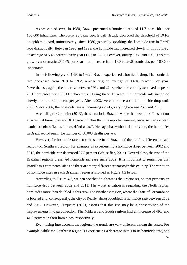
Chapter 4 Homicide in Brazil, Pernambuco, and Recife
52
As we can observe, in 1980, Brazil presented a homicide rate of 11.7 homicides per
100,000 inhabitants. Therefore, 36 years ago, Brazil already exceeded the threshold of 10 for
an epidemic. And, unfortunately, since 1980, generally speaking, the homicide rate in Brazil
rose dramatically. Between 1980 and 1988, the homicide rate increased slowly in this country,
an average of 5.45 percent every year (11.7 to 16.8). However, during 1988 and 1990, this rate
grew by a dramatic 29.76% per year – an increase from 16.8 to 26.8 homicides per 100,000
inhabitants.
In the following years (1990 to 1992), Brazil experienced a homicide drop. The homicide
rate decreased from 26.8 to 19.2, representing an average of 14.18 percent per year.
Nevertheless, again, the rate rose between 1992 and 2003, when the country achieved its peak:
29.1 homicides per 100,000 inhabitants. During these 11 years, the homicide rate increased
slowly, about 4.69 percent per year. After 2003, we can notice a small homicide drop until
2005. Since 2006, the homicide rate is increasing slowly, varying between 25.5 and 27.8.
According to Cerqueira (2013), the scenario in Brazil is worse than we think. This author
affirms that homicides are 18.3 percent higher than the reported amount, because many violent
deaths are classified as “unspecified cause”. He says that without this mistake, the homicides
in Brazil would reach the number of 60,000 deaths per year.
However, the homicide rate is not the same in all Brazil and the trend is different in each
region too. Southeast region, for example, is experiencing a homicide drop: between 2002 and
2012, the homicide rate decreased 37.5 percent (Waiselfisz, 2014). Nevertheless, the rest of the
Brazilian regions presented homicide increase since 2002. It is important to remember that
Brazil has a continental size and there are many different scenarios in this country. The variation
of homicide rates in each Brazilian region is showed in Figure 4.2 below.
According to Figure 4.2, we can see that Southeast is the unique region that presents an
homicide drop between 2002 and 2012. The worst situation is regarding the North region:
homicides more than doubled in this area. The Northeast region, where the State of Pernambuco
is located and, consequently, the city of Recife, almost doubled its homicide rate between 2002
and 2012. However, Cerqueira (2013) asserts that this rise may be a consequence of the
improvements in data collection. The Midwest and South regions had an increase of 49.8 and
41.2 percent in their homicides, respectively.
Even taking into account the regions, the trends are very different among the states. For
example: while the Southeast region is experiencing a decrease in this in its homicide rate, one
Chapter 4 Homicide in Brazil, Pernambuco, and Recife
53
state is presenting a increase: Espírito Santo State – 3.3 percent. Furthermore, while Northeast
region has a homicide rise, Pernambuco State is presenting a drop: Pernambuco – 25.2 percent.
Because of these peculiarities, we decided to show the variations in homicide rates by states in
Figure 4.3, also considering 2002 to 2012.
Figure 4.2 - Variation of homicides in Brazil by region (2002 – 2012)
Source: Waiselfisz, 2014 (primary data).
As can be seen in Figure 4.3, the variation in homicide rates is significant within Brazil.
Although the homicide rise being almost a rule in this country, the results of five states need to
be highlighted. The states of Mato Grosso do Sul, Rondônia, Pernambuco, São Paulo, and Rio
de Janeiro are experiencing a homicide drop. These states alone comprised 35 percent of the
Brazilian population in 2012. The greatest magnitude of homicide drops in Brazil occurred in
São Paulo and Rio de Janeiro, the 1st and 3rd states of the country in population, respectively.
Regarding the states that experienced a homicide rise, we can comment that the three
worst variations are from the Northeast region. Rio Grande do Norte state has the most
pessimistic situation in the period: this region almost increased its homicide rate three times.
Bahia state increased almost 2,5 times and Maranhão, 2 times. It is importante to notice that
Maranhão and Rio Grande do Note, however, do not have the highest homicide rates of Brazil.
These states are in 24th and 12th positions in the ranking, respectevely. The homicide rates of
all Brazilian states can be found in Table 4.1.
Table 4.1 shows the homicide rates in descending order. Among the first five states with
the highest homicide rates, three are from Northeast region (Alagoas, Bahia, and Ceará), one
from Southeast (Espírito Santo), and one from Midwest (Goiás) . Alagoas’s homicide rate was
64.6 homicides per 100,000 inhabitants in 2012 and this state more than doubled its homicide
-37.5
41.2
49.8
91.5
107.6
Southeast
South
Midwest
Northeast
North
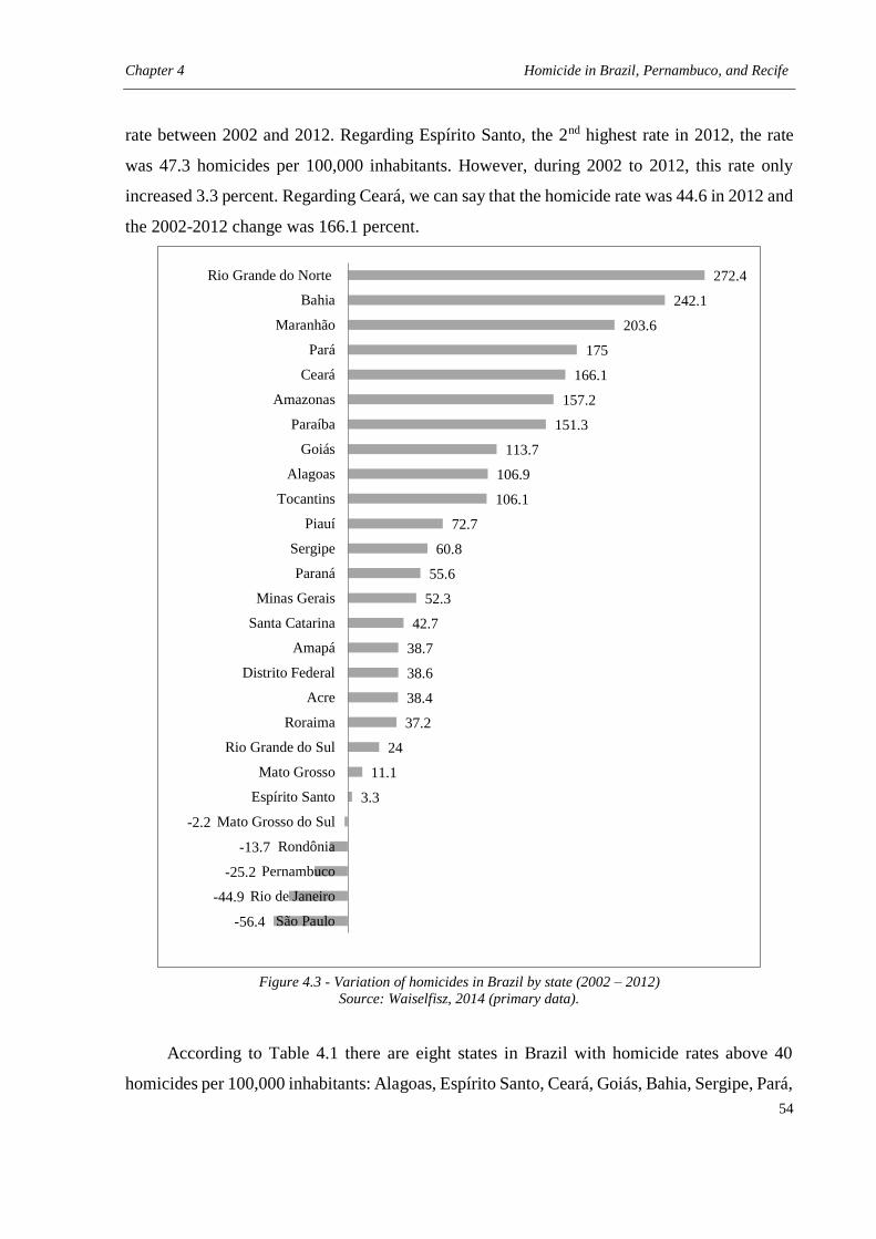
Chapter 4 Homicide in Brazil, Pernambuco, and Recife
54
rate between 2002 and 2012. Regarding Espírito Santo, the 2nd highest rate in 2012, the rate
was 47.3 homicides per 100,000 inhabitants. However, during 2002 to 2012, this rate only
increased 3.3 percent. Regarding Ceará, we can say that the homicide rate was 44.6 in 2012 and
the 2002-2012 change was 166.1 percent.
Figure 4.3 - Variation of homicides in Brazil by state (2002 – 2012)
Source: Waiselfisz, 2014 (primary data).
According to Table 4.1 there are eight states in Brazil with homicide rates above 40
homicides per 100,000 inhabitants: Alagoas, Espírito Santo, Ceará, Goiás, Bahia, Sergipe, Pará,
-56.4
-44.9
-25.2
-13.7
-2.2
3.3
11.1
24
37.2
38.4
38.6
38.7
42.7
52.3
55.6
60.8
72.7
106.1
106.9
113.7
151.3
157.2
166.1
175
203.6
242.1
272.4
São Paulo
Rio de Janeiro
Pernambuco
Rondônia
Mato Grosso do Sul
Espírito Santo
Mato Grosso
Rio Grande do Sul
Roraima
Acre
Distrito Federal
Amapá
Santa Catarina
Minas Gerais
Paraná
Sergipe
Piauí
Tocantins
Alagoas
Goiás
Paraíba
Amazonas
Ceará
Pará
Maranhão
Bahia
Rio Grande do Norte
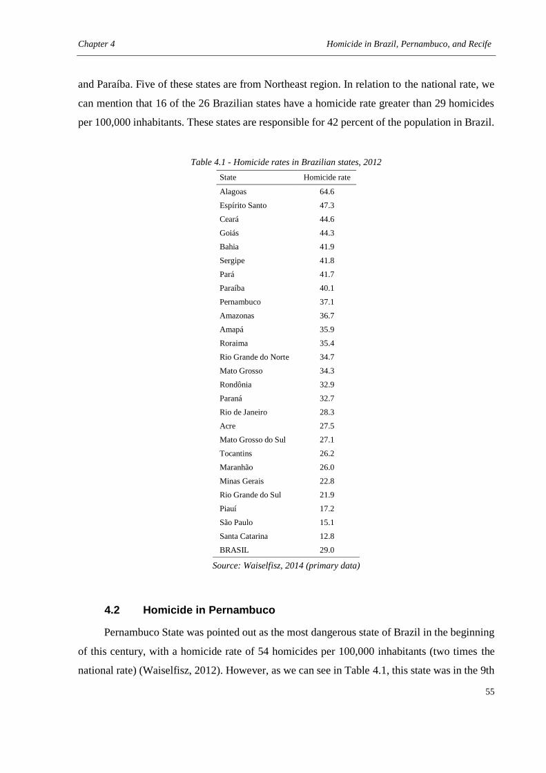
Chapter 4 Homicide in Brazil, Pernambuco, and Recife
55
and Paraíba. Five of these states are from Northeast region. In relation to the national rate, we
can mention that 16 of the 26 Brazilian states have a homicide rate greater than 29 homicides
per 100,000 inhabitants. These states are responsible for 42 percent of the population in Brazil.
Table 4.1 - Homicide rates in Brazilian states, 2012
State Homicide rate
Alagoas 64.6
Espírito Santo 47.3
Ceará 44.6
Goiás 44.3
Bahia 41.9
Sergipe 41.8
Pará 41.7
Paraíba 40.1
Pernambuco 37.1
Amazonas 36.7
Amapá 35.9
Roraima 35.4
Rio Grande do Norte 34.7
Mato Grosso 34.3
Rondônia 32.9
Paraná 32.7
Rio de Janeiro 28.3
Acre 27.5
Mato Grosso do Sul 27.1
Tocantins 26.2
Maranhão 26.0
Minas Gerais 22.8
Rio Grande do Sul 21.9
Piauí 17.2
São Paulo 15.1
Santa Catarina 12.8
BRASIL 29.0
Source: Waiselfisz, 2014 (primary data)
4.2 Homicide in Pernambuco
Pernambuco State was pointed out as the most dangerous state of Brazil in the beginning
of this century, with a homicide rate of 54 homicides per 100,000 inhabitants (two times the
national rate) (Waiselfisz, 2012). However, as we can see in Table 4.1, this state was in the 9th
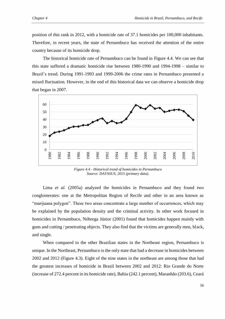
Chapter 4 Homicide in Brazil, Pernambuco, and Recife
56
position of this rank in 2012, with a homicide rate of 37.1 homicides per 100,000 inhabitants.
Therefore, in recent years, the state of Pernambuco has received the attention of the entire
country because of its homicide drop.
The historical homicide rate of Pernambuco can be found in Figure 4.4. We can see that
this state suffered a dramatic homicide rise between 1980-1990 and 1994-1998 – similar to
Brazil’s trend. During 1991-1993 and 1999-2006 the crime rates in Pernambuco presented a
mixed fluctuation. However, in the end of this historical data we can observe a homicide drop
that began in 2007.
Figure 4.4 - Historical trend of homicides in Pernambuco
Source: DATASUS, 2015 (primary data).
Lima et al. (2005a) analyzed the homicides in Pernambuco and they found two
conglomerates: one at the Metropolitan Region of Recife and other in an area known as
“marijuana polygon”. These two areas concentrate a large number of occurrences, which may
be explained by the population density and the criminal activity. In other work focused in
homicides in Pernambuco, Nóbrega Júnior (2001) found that homicides happen mainly with
guns and cutting / penetrating objects. They also find that the victims are generally men, black,
and single.
When compared to the other Brazilian states in the Northeast region, Pernambuco is
unique. In the Northeast, Pernambuco is the only state that had a decrease in homicides between
2002 and 2012 (Figure 4.3). Eight of the nine states in the northeast are among those that had
the greatest increases of homicide in Brazil between 2002 and 2012: Rio Grande do Norte
(increase of 272.4 percent in its homicide rate), Bahia (242.1 percent), Maranhão (203.6), Ceará
0
10
20
30
40
50
60
1980
1982
1984
1986
1988
1990
1992
1994
1996
1998
2000
2002
2004
2006
2008
2010
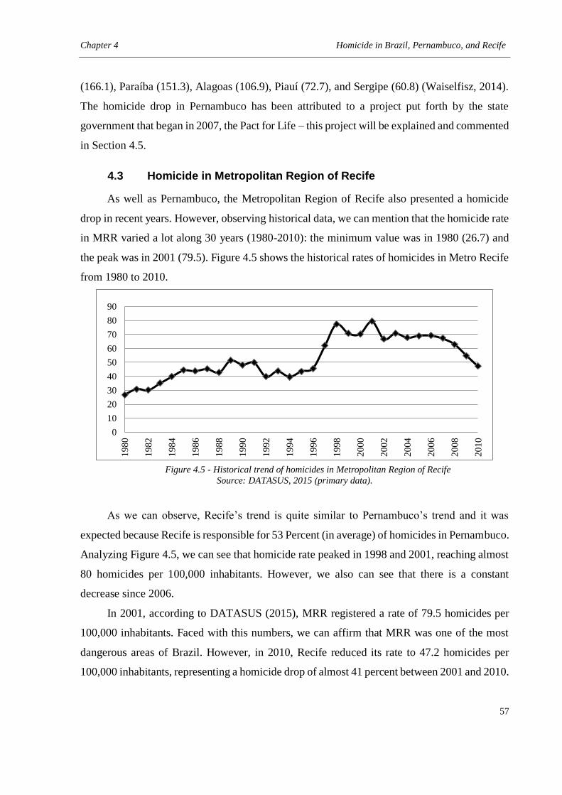
Chapter 4 Homicide in Brazil, Pernambuco, and Recife
57
(166.1), Paraíba (151.3), Alagoas (106.9), Piauí (72.7), and Sergipe (60.8) (Waiselfisz, 2014).
The homicide drop in Pernambuco has been attributed to a project put forth by the state
government that began in 2007, the Pact for Life – this project will be explained and commented
in Section 4.5.
4.3 Homicide in Metropolitan Region of Recife
As well as Pernambuco, the Metropolitan Region of Recife also presented a homicide
drop in recent years. However, observing historical data, we can mention that the homicide rate
in MRR varied a lot along 30 years (1980-2010): the minimum value was in 1980 (26.7) and
the peak was in 2001 (79.5). Figure 4.5 shows the historical rates of homicides in Metro Recife
from 1980 to 2010.
Figure 4.5 - Historical trend of homicides in Metropolitan Region of Recife
Source: DATASUS, 2015 (primary data).
As we can observe, Recife’s trend is quite similar to Pernambuco’s trend and it was
expected because Recife is responsible for 53 Percent (in average) of homicides in Pernambuco.
Analyzing Figure 4.5, we can see that homicide rate peaked in 1998 and 2001, reaching almost
80 homicides per 100,000 inhabitants. However, we also can see that there is a constant
decrease since 2006.
In 2001, according to DATASUS (2015), MRR registered a rate of 79.5 homicides per
100,000 inhabitants. Faced with this numbers, we can affirm that MRR was one of the most
dangerous areas of Brazil. However, in 2010, Recife reduced its rate to 47.2 homicides per
100,000 inhabitants, representing a homicide drop of almost 41 percent between 2001 and 2010.
0
10
20
30
40
50
60
70
80
90
1980
1982
1984
1986
1988
1990
1992
1994
1996
1998
2000
2002
2004
2006
2008
2010
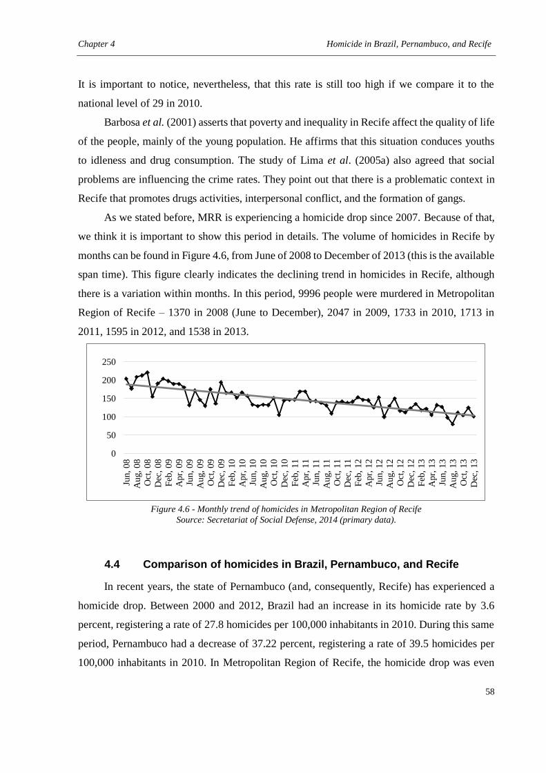
Chapter 4 Homicide in Brazil, Pernambuco, and Recife
58
It is important to notice, nevertheless, that this rate is still too high if we compare it to the
national level of 29 in 2010.
Barbosa et al. (2001) asserts that poverty and inequality in Recife affect the quality of life
of the people, mainly of the young population. He affirms that this situation conduces youths
to idleness and drug consumption. The study of Lima et al. (2005a) also agreed that social
problems are influencing the crime rates. They point out that there is a problematic context in
Recife that promotes drugs activities, interpersonal conflict, and the formation of gangs.
As we stated before, MRR is experiencing a homicide drop since 2007. Because of that,
we think it is important to show this period in details. The volume of homicides in Recife by
months can be found in Figure 4.6, from June of 2008 to December of 2013 (this is the available
span time). This figure clearly indicates the declining trend in homicides in Recife, although
there is a variation within months. In this period, 9996 people were murdered in Metropolitan
Region of Recife – 1370 in 2008 (June to December), 2047 in 2009, 1733 in 2010, 1713 in
2011, 1595 in 2012, and 1538 in 2013.
Figure 4.6 - Monthly trend of homicides in Metropolitan Region of Recife
Source: Secretariat of Social Defense, 2014 (primary data).
4.4 Comparison of homicides in Brazil, Pernambuco, and Recife
In recent years, the state of Pernambuco (and, consequently, Recife) has experienced a
homicide drop. Between 2000 and 2012, Brazil had an increase in its homicide rate by 3.6
percent, registering a rate of 27.8 homicides per 100,000 inhabitants in 2010. During this same
period, Pernambuco had a decrease of 37.22 percent, registering a rate of 39.5 homicides per
100,000 inhabitants in 2010. In Metropolitan Region of Recife, the homicide drop was even
0
50
100
150
200
250
Jun, 08
Aug, 08
Oct
, 08
Dec
, 08
Feb
, 09
Apr,
09
Jun, 09
Aug, 09
Oct
, 09
Dec
, 09
Feb
, 10
Apr,
10
Jun, 10
Aug, 10
Oct
, 10
Dec
, 10
Feb
, 11
Apr,
11
Jun, 11
Aug, 11
Oct
, 11
Dec
, 11
Feb
, 12
Apr,
12
Jun, 12
Aug, 12
Oct
, 12
Dec
, 12
Feb
, 13
Apr,
13
Jun, 13
Aug, 13
Oct
, 13
Dec
, 13
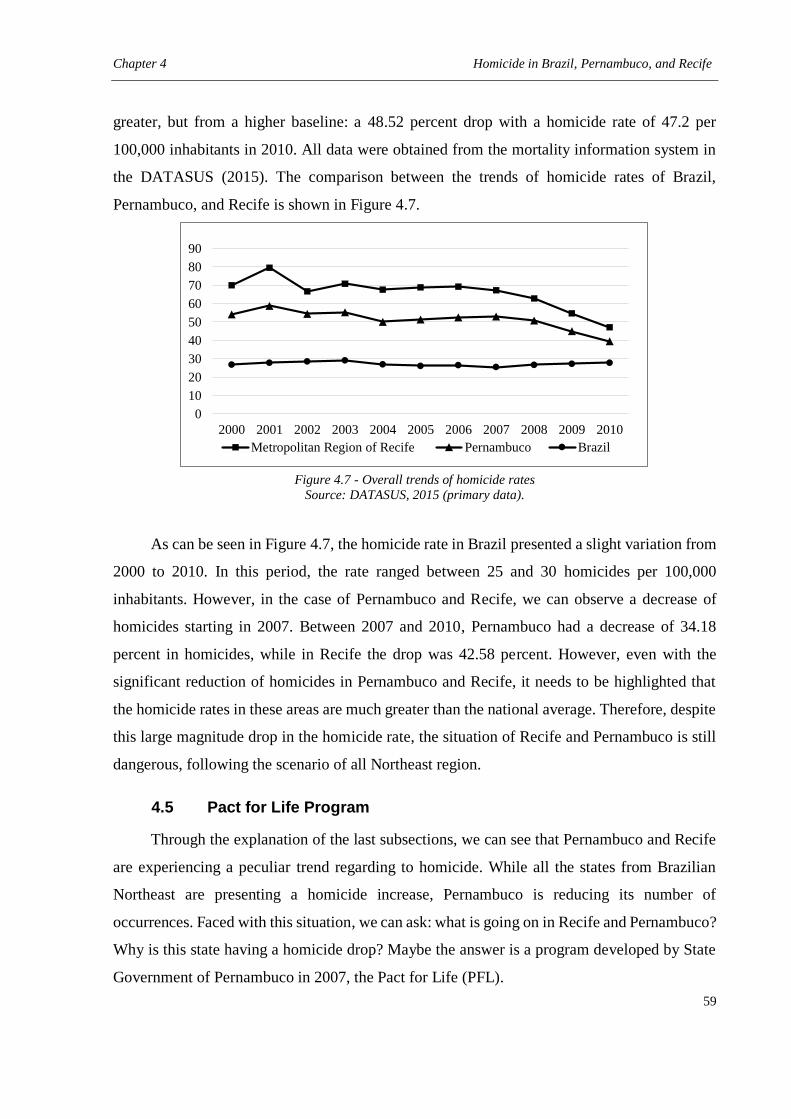
Chapter 4 Homicide in Brazil, Pernambuco, and Recife
59
greater, but from a higher baseline: a 48.52 percent drop with a homicide rate of 47.2 per
100,000 inhabitants in 2010. All data were obtained from the mortality information system in
the DATASUS (2015). The comparison between the trends of homicide rates of Brazil,
Pernambuco, and Recife is shown in Figure 4.7.
Figure 4.7 - Overall trends of homicide rates
Source: DATASUS, 2015 (primary data).
As can be seen in Figure 4.7, the homicide rate in Brazil presented a slight variation from
2000 to 2010. In this period, the rate ranged between 25 and 30 homicides per 100,000
inhabitants. However, in the case of Pernambuco and Recife, we can observe a decrease of
homicides starting in 2007. Between 2007 and 2010, Pernambuco had a decrease of 34.18
percent in homicides, while in Recife the drop was 42.58 percent. However, even with the
significant reduction of homicides in Pernambuco and Recife, it needs to be highlighted that
the homicide rates in these areas are much greater than the national average. Therefore, despite
this large magnitude drop in the homicide rate, the situation of Recife and Pernambuco is still
dangerous, following the scenario of all Northeast region.
4.5 Pact for Life Program
Through the explanation of the last subsections, we can see that Pernambuco and Recife
are experiencing a peculiar trend regarding to homicide. While all the states from Brazilian
Northeast are presenting a homicide increase, Pernambuco is reducing its number of
occurrences. Faced with this situation, we can ask: what is going on in Recife and Pernambuco?
Why is this state having a homicide drop? Maybe the answer is a program developed by State
Government of Pernambuco in 2007, the Pact for Life (PFL).
0
10
20
30
40
50
60
70
80
90
2000 2001 2002 2003 2004 2005 2006 2007 2008 2009 2010
Metropolitan Region of Recife Pernambuco Brazil
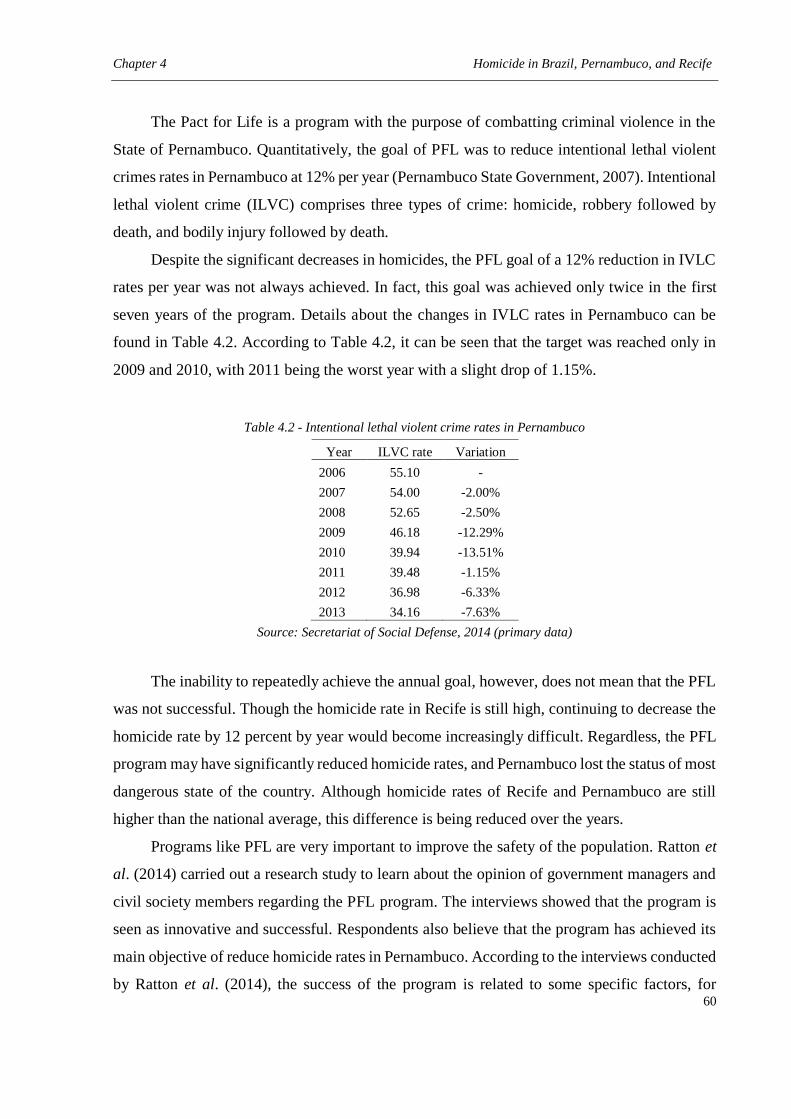
Chapter 4 Homicide in Brazil, Pernambuco, and Recife
60
The Pact for Life is a program with the purpose of combatting criminal violence in the
State of Pernambuco. Quantitatively, the goal of PFL was to reduce intentional lethal violent
crimes rates in Pernambuco at 12% per year (Pernambuco State Government, 2007). Intentional
lethal violent crime (ILVC) comprises three types of crime: homicide, robbery followed by
death, and bodily injury followed by death.
Despite the significant decreases in homicides, the PFL goal of a 12% reduction in IVLC
rates per year was not always achieved. In fact, this goal was achieved only twice in the first
seven years of the program. Details about the changes in IVLC rates in Pernambuco can be
found in Table 4.2. According to Table 4.2, it can be seen that the target was reached only in
2009 and 2010, with 2011 being the worst year with a slight drop of 1.15%.
Table 4.2 - Intentional lethal violent crime rates in Pernambuco
Year ILVC rate Variation
2006 55.10 -
2007 54.00 -2.00%
2008 52.65 -2.50%
2009 46.18 -12.29%
2010 39.94 -13.51%
2011 39.48 -1.15%
2012 36.98 -6.33%
2013 34.16 -7.63%
Source: Secretariat of Social Defense, 2014 (primary data)
The inability to repeatedly achieve the annual goal, however, does not mean that the PFL
was not successful. Though the homicide rate in Recife is still high, continuing to decrease the
homicide rate by 12 percent by year would become increasingly difficult. Regardless, the PFL
program may have significantly reduced homicide rates, and Pernambuco lost the status of most
dangerous state of the country. Although homicide rates of Recife and Pernambuco are still
higher than the national average, this difference is being reduced over the years.
Programs like PFL are very important to improve the safety of the population. Ratton et
al. (2014) carried out a research study to learn about the opinion of government managers and
civil society members regarding the PFL program. The interviews showed that the program is
seen as innovative and successful. Respondents also believe that the program has achieved its
main objective of reduce homicide rates in Pernambuco. According to the interviews conducted
by Ratton et al. (2014), the success of the program is related to some specific factors, for
Chapter 4 Homicide in Brazil, Pernambuco, and Recife
61
example: the strong monitoring of former Governor Eduardo Campos, the new form of
management in the public security area, the use of more reliable data in decision making, and
the integration between police forces.
The receipt of two international awards highlights the success of the Pact for Life
Program. The first award was given by the United Nations into the category of "Improving the
Delivery of Public Services" in 2013. The Inter-American Development Bank awarded the
second award in 2014, in the category "Government Security: preventing crime and violence".
The success of the Pact for Life Program can be understood through its multiple strategy
and multiple year time horizons built into its projects. Because of this structure, the projects
within Pact for Life Program can be classified using the Brantingham & Faust (1976) model of
crime prevention. Brantingham & Faust (1976) developed a conceptual model of crime
prevention that allows the classification of crime prevention actions at three levels: primary,
secondary and tertiary (PST model). Each level has different purposes and it is related to
different time horizons.
The tertiary level involves the prevention of recidivism. Initiatives at this level work with
individuals who have committed crimes, with the hope of preventing the occurrence of new
crimes. For example, these initiatives may include punishment and rehabilitation activities.
These actions have an immediate effect on the crime prevention.
The secondary level is in regard to the identification of potential offenders, and
interventions to prevent them from moving into criminal activities. Brantingham & Faust
(1976) state that this level involves early identification of potential offenders, individual
intervention, and neighborhood programs. The effects of secondary initiatives can be perceived
in a period varying between short and medium term.
Finally, the primary level comprises actions related to change the favorable environment
for crime. According to Brantingham & Faust (1976), primary initiatives involve environmental
design, well-being programs and crime prevention education. Such actions are deeper and its
consequences are perceived in the long run.
The PFL program has initiatives that fit into all levels of the PST model of crime
prevention proposed by Brantingham & Faust (1976). Table 4.3 shows some of the projects that
are part of the program, classifying them according to the PST model. It is worth mentioning
that the PFL involves 138 projects, grouped along six lines of structuring actions: qualified
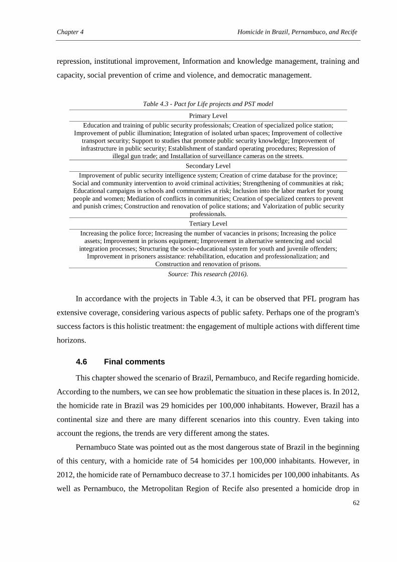
Chapter 4 Homicide in Brazil, Pernambuco, and Recife
62
repression, institutional improvement, Information and knowledge management, training and
capacity, social prevention of crime and violence, and democratic management.
Table 4.3 - Pact for Life projects and PST model
Primary Level
Education and training of public security professionals; Creation of specialized police station;
Improvement of public illumination; Integration of isolated urban spaces; Improvement of collective
transport security; Support to studies that promote public security knowledge; Improvement of
infrastructure in public security; Establishment of standard operating procedures; Repression of
illegal gun trade; and Installation of surveillance cameras on the streets.
Secondary Level
Improvement of public security intelligence system; Creation of crime database for the province;
Social and community intervention to avoid criminal activities; Strengthening of communities at risk;
Educational campaigns in schools and communities at risk; Inclusion into the labor market for young
people and women; Mediation of conflicts in communities; Creation of specialized centers to prevent
and punish crimes; Construction and renovation of police stations; and Valorization of public security
professionals.
Tertiary Level
Increasing the police force; Increasing the number of vacancies in prisons; Increasing the police
assets; Improvement in prisons equipment; Improvement in alternative sentencing and social
integration processes; Structuring the socio-educational system for youth and juvenile offenders;
Improvement in prisoners assistance: rehabilitation, education and professionalization; and
Construction and renovation of prisons.
Source: This research (2016).
In accordance with the projects in Table 4.3, it can be observed that PFL program has
extensive coverage, considering various aspects of public safety. Perhaps one of the program's
success factors is this holistic treatment: the engagement of multiple actions with different time
horizons.
4.6 Final comments
This chapter showed the scenario of Brazil, Pernambuco, and Recife regarding homicide.
According to the numbers, we can see how problematic the situation in these places is. In 2012,
the homicide rate in Brazil was 29 homicides per 100,000 inhabitants. However, Brazil has a
continental size and there are many different scenarios into this country. Even taking into
account the regions, the trends are very different among the states.
Pernambuco State was pointed out as the most dangerous state of Brazil in the beginning
of this century, with a homicide rate of 54 homicides per 100,000 inhabitants. However, in
2012, the homicide rate of Pernambuco decrease to 37.1 homicides per 100,000 inhabitants. As
well as Pernambuco, the Metropolitan Region of Recife also presented a homicide drop in
Chapter 4 Homicide in Brazil, Pernambuco, and Recife
63
recent years. In 2001, MRR registered a rate of 79.5 homicides per 100,000 inhabitants.
However, in 2010, Recife reduced its rate to 47.2 homicides per 100,000 inhabitants,
representing a homicide drop of almost 41 percent between 2001 and 2010.
However, even with the significant reduction of homicides in Pernambuco and Recife, it
needs to be highlighted that the homicide rates in these areas are much greater than the national
average (29 homicides per 100,000 inhabitants). Therefore, despite this large magnitude drop
in the homicide rate, the situation of Recife and Pernambuco is still dangerous.
In 2007, a program was developed by the State Government of Pernambuco, concerned
on reducing violent deaths: Pact for Life. This program is marked by its multiple strategy and
multiple year time horizons built into its projects. Because of this structure, the projects within
Pact for Life Program can be classified using the Brantingham & Faust (1976) model of crime
prevention - Primary, Secondary and Tertiary model.
Chapter 5 Temporal analysis of homicide in Recife
64
5 TEMPORAL ANALYSIS OF HOMICIDE IN RECIFE
The seasonal analysis of crime is an old and controversial debate in the literature with
mixed empirical support. In this sense, this chapter aims to investigate the temporal variations
(seasons, months, days of week, and periods of day) of homicide in Recife.
This analysis contributes to the literature through a study of a tropical climate region, the
consideration of four temporal dimensions, and subsequent spatial analysis. We found no
statistically significant differences between seasons and months, although there is a modest
increase in the hottest months. However, there is a significant increase in homicides during
weekends and evenings.
We also found that the spatial patterns are different within the temporal dimensions,
except for months and some days of week. In addition, the findings indicate that researchers
should not aggregate homicides by year, week, or day when place matters, because spatial
patterns within these dimensions are not similar. Moreover, we conclude that the temporal
variations of homicide in Recife can be understood considering routine activity theory.
5.1 Contextualization
The seasonality of crime is a well-established literature dating back to the mid-1800s, but
with mixed empirical support (Abel et al., 1985; Cheatwood, 1988; Landau & Fridman, 1993;
Tennenbaum & Fink, 1994; Rock et al., 2008; McDowall et al., 2012). Though there is a general
consensus that there is a seasonal component to assault (see, for example, Harries et al., 1984),
this consensus dissipates rather quickly when considering other crime types (Uittenbogaard &
Ceccato, 2012; McDowall et al., 2012). The cited reasons for this lack of consensus in
seasonality results are debated, with some authors considering the different time frames of
analysis and a lack of significant seasonal variations in weather.
There are essentially two theories used to explain the seasonality (of homicide):
temperature/aggression theory and routine activity theory (Cheatwood, 1995; Hipp et al., 2004;
Ceccato, 2005; McDowall et al., 2012). Each theory has its basic premise to explain this
seasonal pattern of homicides: (1) homicides are more frequent during the summer because heat
stimulates aggressive behavior; and (2) homicide patterns are a consequence of increased social
interaction during summer months because of vacations from school and work.
Chapter 5 Temporal analysis of homicide in Recife
65
Temperature/aggression theory was first proposed by Quetelet and “this theory suggests
that hot temperatures lead to greater discomfort, which in turn gives rise to more aggressive
behavior.” (Hipp et al., 2004). Thus, according to this theory, there may be more violent crimes
during hotter days because of higher stress caused by heat. It is important to highlight that this
theory is adequate to explain violent crimes, but not property crimes. Despite this limitation of
its application, Hipp et al. (2004) assert that there are many works in the literature that give
support to temperature/aggression theory.
Routine activity theory does not suggest that higher temperatures may cause an increase
in homicides because of the aggressive behavior. Rather, routine activity theory posits that
homicides will increase because of changes in routine activities with warmer weather. Routine
activity theory states that crime can occur when three fundamental elements converge in time
and space: a motivated offender, a suitable target, and the lack of capable guardianship (Cohen
& Felson, 1979). In hotter days, people are more likely to enjoy outdoor activities, so the
probability of interaction between motivated offenders and suitable targets is greater. Therefore,
criminal opportunity is greater due to a greater volume of social interactions, as well as the
lower vigilance on property because more people are away from the relatively protective
environment of the home. Consequently, routine activity theory is able to explain both violent
and property crimes, because there is an interaction between a motivated offender and a suitable
target, whether that target be a person or that person’s property.
Some authors suggest that routine activity theory is more appropriate to explain
homicides than temperature/aggression theory (Falk, 1952; Anderson, 1987; Cheatwood, 1988;
Landau & Fridman, 1993; Ceccato, 2005; McDowall et al., 2012). On the other hand, Hipp et
al. (2004) asserts that these theories are not mutually exclusive. This study will contribute to
this debate regarding temperature/aggression theory and routine activity theory in the context
of homicide in Recife.
The temporal analysis of homicides has been widely explored in some places, such as the
United States. In fact, Ceccato (2005) asserts that this research is dominated by studies
undertaken in temperate climates, with few papers considering hotter climates. However, there
is an increasing body of research on homicides in hotter climates; more generally, the temporal
dimension of crime literature has expanded with significant research undertaken in other
contexts, including the developing world – see, for example, Breetzke & Cohn (2012),
Uittenbogaard & Ceccato (2012), and Breetzke (2015). In this sense, this work investigates the
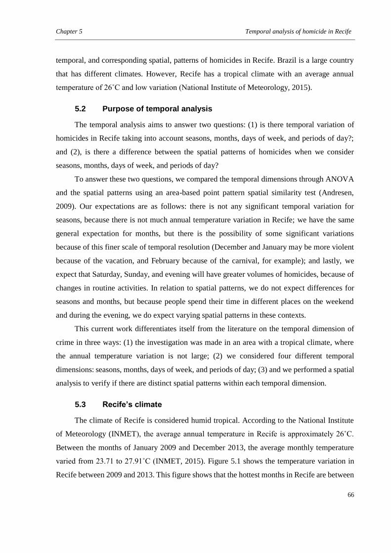
Chapter 5 Temporal analysis of homicide in Recife
66
temporal, and corresponding spatial, patterns of homicides in Recife. Brazil is a large country
that has different climates. However, Recife has a tropical climate with an average annual
temperature of 26˚C and low variation (National Institute of Meteorology, 2015).
5.2 Purpose of temporal analysis
The temporal analysis aims to answer two questions: (1) is there temporal variation of
homicides in Recife taking into account seasons, months, days of week, and periods of day?;
and (2), is there a difference between the spatial patterns of homicides when we consider
seasons, months, days of week, and periods of day?
To answer these two questions, we compared the temporal dimensions through ANOVA
and the spatial patterns using an area-based point pattern spatial similarity test (Andresen,
2009). Our expectations are as follows: there is not any significant temporal variation for
seasons, because there is not much annual temperature variation in Recife; we have the same
general expectation for months, but there is the possibility of some significant variations
because of this finer scale of temporal resolution (December and January may be more violent
because of the vacation, and February because of the carnival, for example); and lastly, we
expect that Saturday, Sunday, and evening will have greater volumes of homicides, because of
changes in routine activities. In relation to spatial patterns, we do not expect differences for
seasons and months, but because people spend their time in different places on the weekend
and during the evening, we do expect varying spatial patterns in these contexts.
This current work differentiates itself from the literature on the temporal dimension of
crime in three ways: (1) the investigation was made in an area with a tropical climate, where
the annual temperature variation is not large; (2) we considered four different temporal
dimensions: seasons, months, days of week, and periods of day; (3) and we performed a spatial
analysis to verify if there are distinct spatial patterns within each temporal dimension.
5.3 Recife’s climate
The climate of Recife is considered humid tropical. According to the National Institute
of Meteorology (INMET), the average annual temperature in Recife is approximately 26˚C.
Between the months of January 2009 and December 2013, the average monthly temperature
varied from 23.71 to 27.91˚C (INMET, 2015). Figure 5.1 shows the temperature variation in
Recife between 2009 and 2013. This figure shows that the hottest months in Recife are between
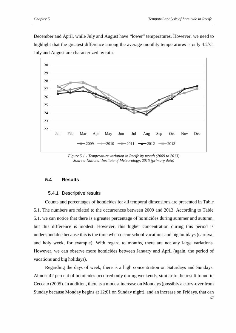
Chapter 5 Temporal analysis of homicide in Recife
67
December and April, while July and August have “lower” temperatures. However, we need to
highlight that the greatest difference among the average monthly temperatures is only 4.2˚C.
July and August are characterized by rain.
Figure 5.1 - Temperature variation in Recife by month (2009 to 2013)
Source: National Institute of Meteorology, 2015 (primary data)
5.4 Results
5.4.1 Descriptive results
Counts and percentages of homicides for all temporal dimensions are presented in Table
5.1. The numbers are related to the occurrences between 2009 and 2013. According to Table
5.1, we can notice that there is a greater percentage of homicides during summer and autumn,
but this difference is modest. However, this higher concentration during this period is
understandable because this is the time when occur school vacations and big holidays (carnival
and holy week, for example). With regard to months, there are not any large variations.
However, we can observe more homicides between January and April (again, the period of
vacations and big holidays).
Regarding the days of week, there is a high concentration on Saturdays and Sundays.
Almost 42 percent of homicides occurred only during weekends, similar to the result found in
Ceccato (2005). In addition, there is a modest increase on Mondays (possibly a carry-over from
Sunday because Monday begins at 12:01 on Sunday night), and an increase on Fridays, that can
22
23
24
25
26
27
28
29
30
Jan Feb Mar Apr May Jun Jul Aug Sep Oct Nov Dec
2009 2010 2011 2012 2013
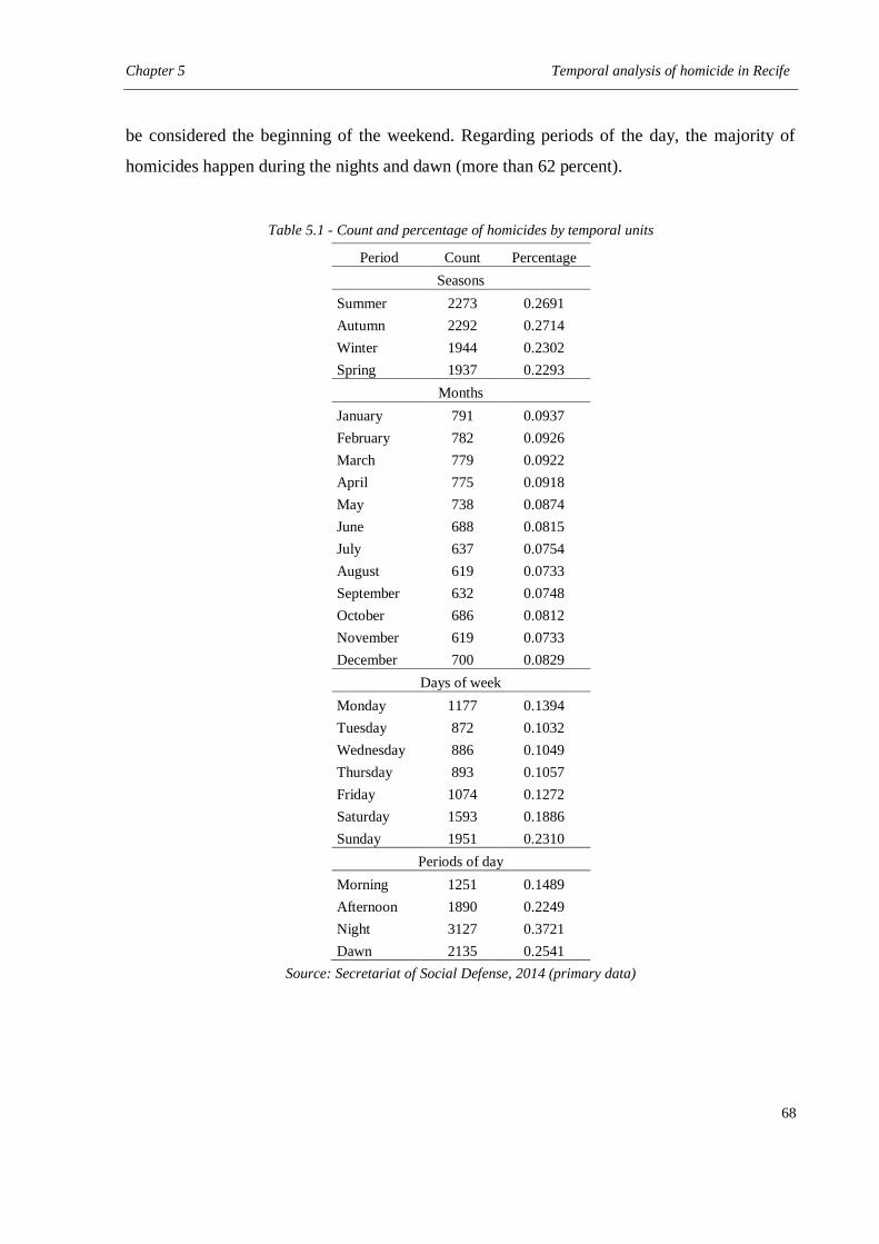
Chapter 5 Temporal analysis of homicide in Recife
68
be considered the beginning of the weekend. Regarding periods of the day, the majority of
homicides happen during the nights and dawn (more than 62 percent).
Table 5.1 - Count and percentage of homicides by temporal units
Period Count Percentage
Seasons
Summer 2273 0.2691
Autumn 2292 0.2714
Winter 1944 0.2302
Spring 1937 0.2293
Months
January 791 0.0937
February 782 0.0926
March 779 0.0922
April 775 0.0918
May 738 0.0874
June 688 0.0815
July 637 0.0754
August 619 0.0733
September 632 0.0748
October 686 0.0812
November 619 0.0733
December 700 0.0829
Days of week
Monday 1177 0.1394
Tuesday 872 0.1032
Wednesday 886 0.1049
Thursday 893 0.1057
Friday 1074 0.1272
Saturday 1593 0.1886
Sunday 1951 0.2310
Periods of day
Morning 1251 0.1489
Afternoon 1890 0.2249
Night 3127 0.3721
Dawn 2135 0.2541
Source: Secretariat of Social Defense, 2014 (primary data)

Chapter 5 Temporal analysis of homicide in Recife
69
5.4.2 ANOVA results
As discussed above, the results in Table 5.1 indicate that there are differences between
the percentages for each temporal dimension. However, in order to test the significance of these
differences, we applied ANOVA. The results are shown in Table 5.2.
Table 5.2 - Results from ANOVA
Temporal dimension F statistics Significance
Seasons 1.7410 0.1989
Months 1.3768 0.2146
Days of week 20.3078 0.0000
Periods of day 24.8013 0.0000
Source: This research (2016)
According to the ANOVA results, the differences cannot be considered statistically
significant for seasons and months; while the variation between days of week and periods of
day are statistically significant. However, there may be particular differences that are
statistically significant and do not emerge in the aggregate ANOVA results (seasons and
months) and, correspondingly, there may be particular differences that are not statistically
significant in the aggregate ANOVA results that may prove to be instructive. In order to test
these hypotheses, we undertake post-hoc ANOVA.
The post-hoc ANOVA confirm the more general results. There are no statistically
significant differences when comparing the individual seasons and months. However,
statistically significant results do emerge for days of week and periods of day. Specifically, for
days of week, both Saturday and Sunday merge as statistically significant from the other days
of the week, but Saturday and Sunday do not have a statistically difference. With regard to the
period of day, aside from afternoon-dawn all comparisons show a statistically significant
difference.
Overall, these results show the importance of considering multiple temporal scales
within the same analysis. When considering more aggregate temporal scales (seasons and
months) we do find increases in the volume of homicides at the expected times of the year, but
those increases are not statistically significant. Only when we consider within week and within
day variation do statistically significant differences emerge. Consequently, homicides in Recife
do not provide much support temperature aggression theory. Rather, the volume of homicides
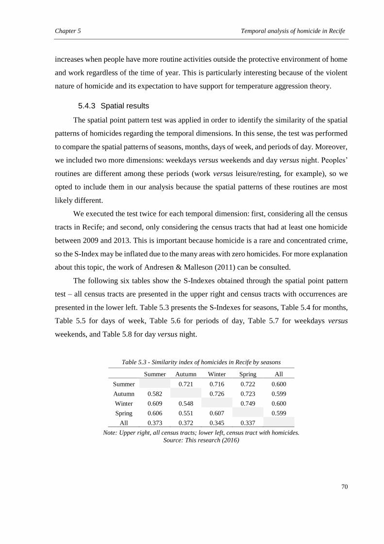
Chapter 5 Temporal analysis of homicide in Recife
70
increases when people have more routine activities outside the protective environment of home
and work regardless of the time of year. This is particularly interesting because of the violent
nature of homicide and its expectation to have support for temperature aggression theory.
5.4.3 Spatial results
The spatial point pattern test was applied in order to identify the similarity of the spatial
patterns of homicides regarding the temporal dimensions. In this sense, the test was performed
to compare the spatial patterns of seasons, months, days of week, and periods of day. Moreover,
we included two more dimensions: weekdays versus weekends and day versus night. Peoples’
routines are different among these periods (work versus leisure/resting, for example), so we
opted to include them in our analysis because the spatial patterns of these routines are most
likely different.
We executed the test twice for each temporal dimension: first, considering all the census
tracts in Recife; and second, only considering the census tracts that had at least one homicide
between 2009 and 2013. This is important because homicide is a rare and concentrated crime,
so the S-Index may be inflated due to the many areas with zero homicides. For more explanation
about this topic, the work of Andresen & Malleson (2011) can be consulted.
The following six tables show the S-Indexes obtained through the spatial point pattern
test – all census tracts are presented in the upper right and census tracts with occurrences are
presented in the lower left. Table 5.3 presents the S-Indexes for seasons, Table 5.4 for months,
Table 5.5 for days of week, Table 5.6 for periods of day, Table 5.7 for weekdays versus
weekends, and Table 5.8 for day versus night.
Table 5.3 - Similarity index of homicides in Recife by seasons
Summer Autumn Winter Spring All
Summer 0.721 0.716 0.722 0.600
Autumn 0.582 0.726 0.723 0.599
Winter 0.609 0.548 0.749 0.600
Spring 0.606 0.551 0.607 0.599
All 0.373 0.372 0.345 0.337
Note: Upper right, all census tracts; lower left, census tract with homicides.
Source: This research (2016)
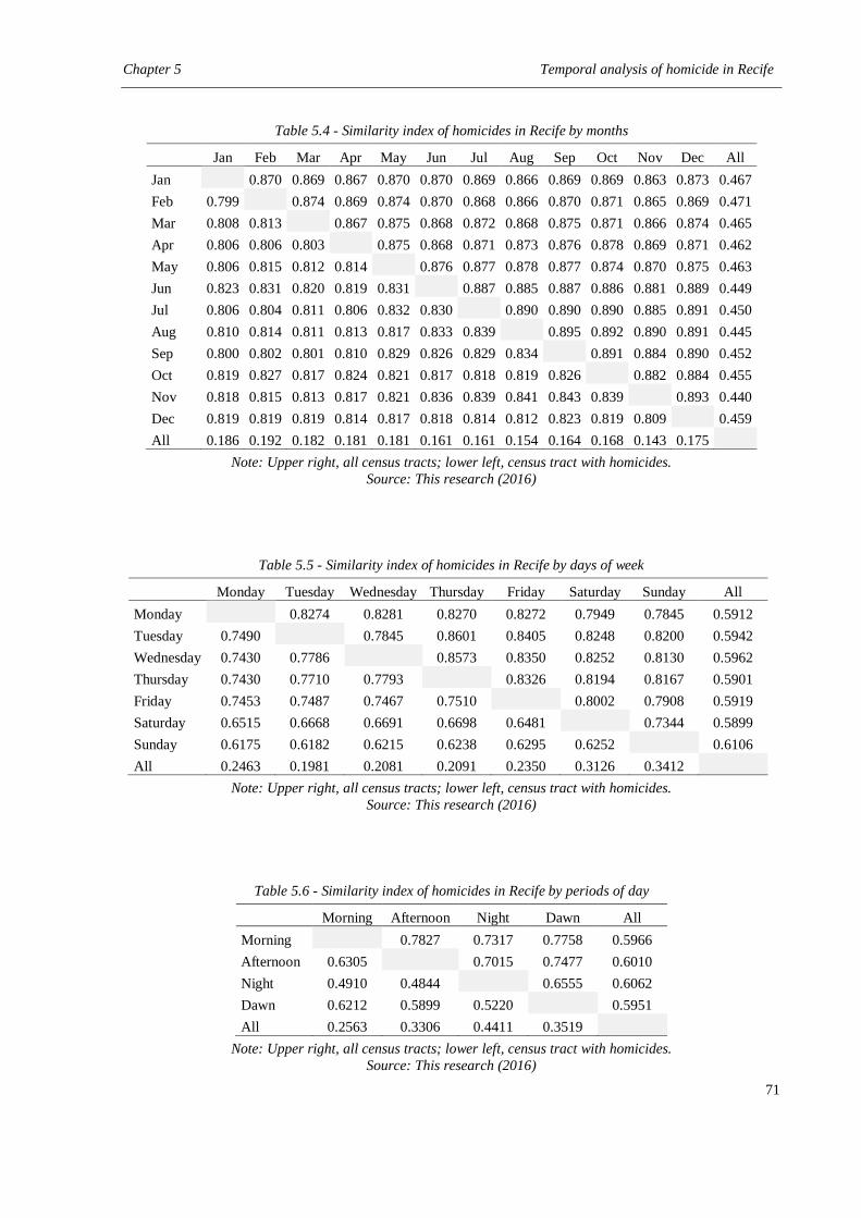
Chapter 5 Temporal analysis of homicide in Recife
71
Table 5.4 - Similarity index of homicides in Recife by months
Jan Feb Mar Apr May Jun Jul Aug Sep Oct Nov Dec All
Jan 0.870 0.869 0.867 0.870 0.870 0.869 0.866 0.869 0.869 0.863 0.873 0.467
Feb 0.799 0.874 0.869 0.874 0.870 0.868 0.866 0.870 0.871 0.865 0.869 0.471
Mar 0.808 0.813 0.867 0.875 0.868 0.872 0.868 0.875 0.871 0.866 0.874 0.465
Apr 0.806 0.806 0.803 0.875 0.868 0.871 0.873 0.876 0.878 0.869 0.871 0.462
May 0.806 0.815 0.812 0.814 0.876 0.877 0.878 0.877 0.874 0.870 0.875 0.463
Jun 0.823 0.831 0.820 0.819 0.831 0.887 0.885 0.887 0.886 0.881 0.889 0.449
Jul 0.806 0.804 0.811 0.806 0.832 0.830 0.890 0.890 0.890 0.885 0.891 0.450
Aug 0.810 0.814 0.811 0.813 0.817 0.833 0.839 0.895 0.892 0.890 0.891 0.445
Sep 0.800 0.802 0.801 0.810 0.829 0.826 0.829 0.834 0.891 0.884 0.890 0.452
Oct 0.819 0.827 0.817 0.824 0.821 0.817 0.818 0.819 0.826 0.882 0.884 0.455
Nov 0.818 0.815 0.813 0.817 0.821 0.836 0.839 0.841 0.843 0.839 0.893 0.440
Dec 0.819 0.819 0.819 0.814 0.817 0.818 0.814 0.812 0.823 0.819 0.809 0.459
All 0.186 0.192 0.182 0.181 0.181 0.161 0.161 0.154 0.164 0.168 0.143 0.175
Note: Upper right, all census tracts; lower left, census tract with homicides.
Source: This research (2016)
Table 5.5 - Similarity index of homicides in Recife by days of week
Monday Tuesday Wednesday Thursday Friday Saturday Sunday All
Monday 0.8274 0.8281 0.8270 0.8272 0.7949 0.7845 0.5912
Tuesday 0.7490 0.7845 0.8601 0.8405 0.8248 0.8200 0.5942
Wednesday 0.7430 0.7786 0.8573 0.8350 0.8252 0.8130 0.5962
Thursday 0.7430 0.7710 0.7793 0.8326 0.8194 0.8167 0.5901
Friday 0.7453 0.7487 0.7467 0.7510 0.8002 0.7908 0.5919
Saturday 0.6515 0.6668 0.6691 0.6698 0.6481 0.7344 0.5899
Sunday 0.6175 0.6182 0.6215 0.6238 0.6295 0.6252 0.6106
All 0.2463 0.1981 0.2081 0.2091 0.2350 0.3126 0.3412
Note: Upper right, all census tracts; lower left, census tract with homicides.
Source: This research (2016)
Table 5.6 - Similarity index of homicides in Recife by periods of day
Morning Afternoon Night Dawn All
Morning 0.7827 0.7317 0.7758 0.5966
Afternoon 0.6305 0.7015 0.7477 0.6010
Night 0.4910 0.4844 0.6555 0.6062
Dawn 0.6212 0.5899 0.5220 0.5951
All 0.2563 0.3306 0.4411 0.3519
Note: Upper right, all census tracts; lower left, census tract with homicides.
Source: This research (2016)
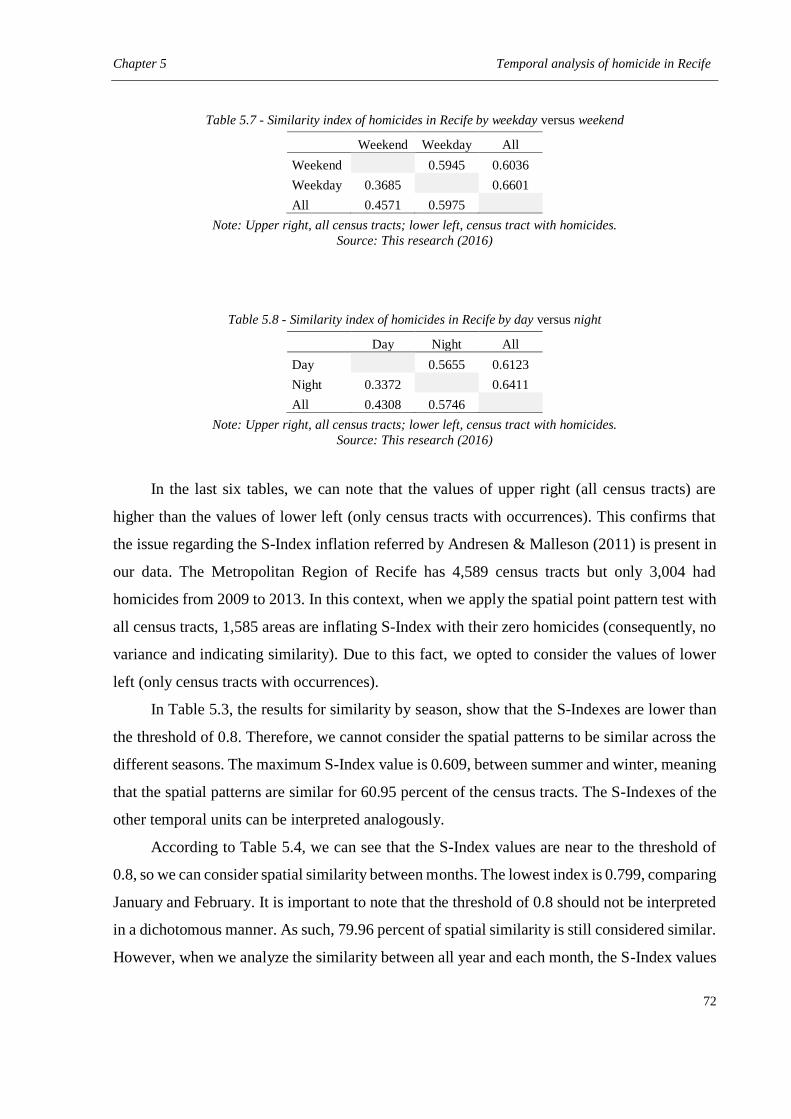
Chapter 5 Temporal analysis of homicide in Recife
72
Table 5.7 - Similarity index of homicides in Recife by weekday versus weekend
Weekend Weekday All
Weekend 0.5945 0.6036
Weekday 0.3685 0.6601
All 0.4571 0.5975
Note: Upper right, all census tracts; lower left, census tract with homicides.
Source: This research (2016)
Table 5.8 - Similarity index of homicides in Recife by day versus night
Day Night All
Day 0.5655 0.6123
Night 0.3372 0.6411
All 0.4308 0.5746
Note: Upper right, all census tracts; lower left, census tract with homicides.
Source: This research (2016)
In the last six tables, we can note that the values of upper right (all census tracts) are
higher than the values of lower left (only census tracts with occurrences). This confirms that
the issue regarding the S-Index inflation referred by Andresen & Malleson (2011) is present in
our data. The Metropolitan Region of Recife has 4,589 census tracts but only 3,004 had
homicides from 2009 to 2013. In this context, when we apply the spatial point pattern test with
all census tracts, 1,585 areas are inflating S-Index with their zero homicides (consequently, no
variance and indicating similarity). Due to this fact, we opted to consider the values of lower
left (only census tracts with occurrences).
In Table 5.3, the results for similarity by season, show that the S-Indexes are lower than
the threshold of 0.8. Therefore, we cannot consider the spatial patterns to be similar across the
different seasons. The maximum S-Index value is 0.609, between summer and winter, meaning
that the spatial patterns are similar for 60.95 percent of the census tracts. The S-Indexes of the
other temporal units can be interpreted analogously.
According to Table 5.4, we can see that the S-Index values are near to the threshold of
0.8, so we can consider spatial similarity between months. The lowest index is 0.799, comparing
January and February. It is important to note that the threshold of 0.8 should not be interpreted
in a dichotomous manner. As such, 79.96 percent of spatial similarity is still considered similar.
However, when we analyze the similarity between all year and each month, the S-Index values
Chapter 5 Temporal analysis of homicide in Recife
73
decrease significantly (maximum value of 0.192). Thus, when we compare all year and each
month we cannot assume similarity and that the aggregation of homicides to the entire year may
not be appropriate because the spatial patterns are considerably distinct.
For the days of the week, Table 5.5, in some cases we can consider the spatial patterns
similar. Therefore, in some cases, we can assume the spatial similarity between some days of
week, such Tuesday versus Wednesday and Tuesday versus Thursday. However, as we found
for months, the S-Indexes are low when we compare all week and each day (maximum of
0.441). Therefore, we also have indication that the aggregation of homicides by the entire week
is not appropriate due to the differences in the spatial patterns.
Considering periods of the day, weekday versus weekend, and day versus night (Tables
5.6, 5.7, and 5.8), we cannot assume spatial similarity. In all cases, all the indexes are far from
0.8, for all temporal units. Again, this is an evidence that the aggregation of homicides is not
appropriate, by week or by day.
5.5 Discussion
5.5.1 Temporal aggression theory versus routine activity theory
As stated above, the temporal variation of homicide can be understood considering two
theories: temperature/aggression theory and routine activity theory. However, which one fits
better in Recife’s context? Cheatwood (1988) affirms that it is important to know which
approach is more relevant because each one implies different political decisions.
Some research asserts that the temporal variation of homicides is better explained by
routine activity theory rather than temperature/aggression theory (Falk, 1952; Anderson, 1987;
Cheatwood, 1988; Landau & Fridman, 1993; Ceccato, 2005). Therefore, we began with the
working hypothesis that homicide in Recife can be understood with routine activity theory.
The first bit of evidence regarding which theory is more relevant for Recife is based on
the work of Tiihonen and colleagues (1997). These authors say that the aggressive behavior,
due to the high temperatures, is more common in regions far from the Equator (and,
consequently, with large climatic variation). Recife is located near the Equator, with latitude of
8 degrees south, or less than 900 kilometers from the Equator. In Recife, the climatic variation
is not significant and the temperature is high all year (see Figure 5.1), so people who live there
are used to having heat. Because of these geographic and climatic situations, most people are
Chapter 5 Temporal analysis of homicide in Recife
74
not expected to be susceptible to the aggressive behavior caused by heat. This argument,
therefore, weakens the support to temperature/aggression theory, a priori.
In Recife, recently, there was a significant homicide drop. As presented in Chapter 4,
Recife experienced a homicide decrease of 32.67 percent between 2000 and 2010 (DATASUS,
2015). However, during this period, the weather remained the same in the city. This fact also
weakens the support for the hypothesis that temperature/aggression theory is relevant for
understanding homicide in Recife. However, we measured the relationship between homicides
and temperature directly using the Pearson correlation coefficient. We considered the average
monthly temperature between January 2009 and December 2013, and the number of homicides
by month. We found a coefficient of 0.287 with significance of 0.026. Therefore, there is some
evidence that homicides in Recife have a weak relationship with temperature.
Two more facts do not support temperature/aggression theory in Recife’s context. The
first is related to the high concentration of homicides during weekends (42 percent).
Considering this theory, we expected a uniform distribution of homicide during the week,
because the temperature is similar during the week. Temperature/aggression theory cannot
explain this peak during weekends, but routine activity theory can (due to the change in the
activities and subsequently increasing crime opportunity). The second fact is related to the
period of the day. In Recife, the hottest hours of the day is approximately noon and the sunset
is about 6pm, during all year. Considering the theory, we expected more homicides during the
period of intense heat, probably during afternoon. However, the most violent period is after the
sunset, between 6pm and 5:59am (62 percent of homicides).
Faced with those arguments, routine activity theory provides a far better explanation for
homicide in Recife. However, we cannot say that the temperature/aggression model does not
have any influence on homicides in Recife. As stated by Hipp et al. (2004), these theories are
not mutually exclusive, and temperature/aggression theory appears to have some contribution
based on the correlation between temperature and the number of homicides.
5.5.2 Temporal variation
Through ANOVA results, we can affirm that the variations of homicides in Recife by
season and months cannot be considered statistically significant. As mentioned above, there is
not a consensus in the literature regarding the seasonality of homicides, but we can cite some
explanations for these findings in Recife.
Chapter 5 Temporal analysis of homicide in Recife
75
First, based on statements from Hipp and colleagues (2004), the results are consistent
with explanations for temporal variations because we should not expect high seasonality of
crimes in cities where the temperature variation is not large. The temperature variation in Recife
is rather modest: between January 2009 and December 2013, the average monthly temperature
ranged from 23.71 to 27.91˚C (INMET, 2015). This small degree of variation brings an
important consequence: we cannot expect “seasonality” in Recife because there are not any
significant variations in weather or climate during the year – there are no defined seasons in
Recife. Therefore, we cannot say that there is a change in peoples’ behavior because they are
enjoying the summer or protecting themselves of the winter. Outdoor activities, for example,
can be undertaken all year.
Landau & Fridman (1993) cite other factors that support the lack of seasonality in
homicide: (1) there is not a specific period in the year related to homicides, because the reasons
to commit a homicide are independent of the time of year; (2) the meeting between aggressor
and victim is not as dependent on weather as in other crimes, because normally they know each
other; and (3) the decision of commit a homicide will not likely depend on weather conditions,
because homicides are committed by impulse or carefully planned. Though one may argue these
points, as least as global explanations, they do have some relevance for homicide in Recife.
In Recife, the most common reasons to commit a homicide are criminal activities (20.3
percent) and conflicts within the community (18.8 percent) (Sauret, 2012b). Criminal activities
involve, for example, racketeering, gang disputes, and drug problems; while conflicts in the
community involve discussions in general (gone wrong), drunkenness, and personal revenge.
There is not a specific period during the year when these circumstances occur and these are
situations that occur between people who know each other. Moreover, those motivations are
not related to temperature and the reason to commit the crime must be stronger than a small
variation of temperature. Therefore, the arguments pointed out by Landau & Fridman (1993)
are consistent with the context in Recife.
Nevertheless, we have to clarify that our results may be specific to Recife and we cannot
infer it to all Brazil. Brazil is the fifth largest country in the world and many different weather
conditions can be found here. Cheatwood (1995) affirms that we need to be careful when we
generalize local data to national level, as well as when we consider national findings as local
findings. This fits well within the Brazilian context, particularly with the size of the country.
The study of Ceccato (2005), for example, shows seasonality in São Paulo, but this city has
Chapter 5 Temporal analysis of homicide in Recife
76
weather conditions far different from Recife. Seasonal analysis in Brazilian cities should,
therefore, find distinct results due to the large differences in weather across the country.
In relation to our hypotheses, we confirmed a lack of significant temporal variation in
homicides for seasons in Recife. However, our hypothesis that December, January and February
are more dangerous was not confirmed. Although January is the month with more homicides,
the ANOVA tests showed that the difference in relation with other months is not significant,
including post-hoc tests for these months specifically. We expected these months would be
more violent because of the intense social interactions due to Christmas, New Year, vacations,
and carnival.
Considering days of week, we found that the differences are significant. Homicides are
more frequent during the weekend (Saturday and Sunday), concentrating almost 42 percent of
the occurrences. This finding was expected from a routine activity theory perspective because
this is a leisure period: social interactions are more frequent, and we observe more elements
that can be conducive to crime (alcohol consumption, for example). Interviews conducted by
Minayo & Constantino (2012) within the Metropolitan Region of Recife found that most
violence occurs in the context of youths and leisure activities or when prisoners are released.
In our analysis, we also found two days with a higher percentage of homicides than the
others: Monday (13.94 percent) and Friday (12.72 percent). Though Friday may not be
considered a surprise because it is the beginning of the weekend, there is also an explanation
for Monday that is related. Felson & Poulsen (2003) assert that considering midnight as the
division between two days is not relevant for criminologists; these authors suggest that the
criminological day begins at 5am. Many people who go out for leisure activities still are out (in
bars or parties, for example) after midnight. As such, if a homicide occurs after midnight, it is
likely related to activities that started in the night before. As such, Felson & Poulsen suggest
that the criminological day starts at 5am, because this time of the day seems reasonable to
consider that people have finished their day (those who went out) or are starting their days
(those who will work).
Taking into account the criminological day, we can understand why Friday is not the third
highest day with regard to homicides and why Monday has a high volume of occurrences.
Regarding Friday, some homicides that occurred after 12am of Saturday could be related to
activities that started Friday night. However, those occurrences were registered as Saturday
Chapter 5 Temporal analysis of homicide in Recife
77
dawn. Monday has the same logic: some homicides are related to activities that started Sunday
night, but the crime, or its registration, just occurred after 12am on Monday.
Regarding periods of day, our results show that there is a high prevalence of homicides
during nights and dawns. Again, these results are expected according to the literature,
particularly in the context of routine activity theory. During these periods, many people are at
home or sleeping but some people are outside the relatively protective environment of the home
(increasing the opportunity for crime). Moreover, we can also note that there is a difference in
relation to the day – the lack of natural light. Many aggressors may prefer to commit crimes
during the night in order to avoid recognition and detection. In addition, guardianship is reduced
during nights because there are fewer people on the streets, affecting the safety of the
environment.
Therefore, our hypotheses that homicides are more frequent on Saturdays and Sundays
and during nights and dawns are confirmed. In Recife, almost 42 percent of the occurrences
happen during weekends and more than 62 percent during nights and dawns.
5.5.3 Spatial variation
The spatial point pattern test results show that, generally speaking, there is no spatial
similarity between the temporal dimensions. In relation to seasons, the greatest value S-Index
is 0.609 (between summer and winter) and because of that, we cannot consider that the spatial
patterns between seasons are similar. Moreover, when we compare all year and each season,
the similarity is even lower: the maximum value is 0.373 (37.3 percent of similarity across
census tracts).
Andresen & Malleson (2013) also analyzed the pattern changes in relation to seasons, for
Vancouver, Canada. The largest S-Index they found was 0.515, considering many crimes and
comparing all year with each season. The authors concluded that the aggregation of occurrences
by year is not appropriate because the patterns are dissimilar. They suggested that this analysis
should be replicated in other locations with the purpose to discover if this finding was specific
to Vancouver or generalizable to other locations. For Recife, we can say that the conclusions
are the same. Recife also has different spatial patterns by seasons and the aggregation of
homicides does not seem appropriate when place matters.
Regarding months, we found that there is similarity between the spatial patterns, because
the lowest value S-Index was 0.799, considering month-to-month comparisons. However, the
Chapter 5 Temporal analysis of homicide in Recife
78
similarity cannot be assumed when each month is compared to all year aggregation. In this
analysis, the greatest value S-Index was 0.192 for February that means only 19.21 percent of
the spatial pattern of February is similar to the annual pattern. Because of this percentage being
so low, we can assert that the annual aggregation of homicide data is not appropriate if one is
explicitly or implicitly interested in the spatial patterns of homicide.
Considering days of week, we found mixed results. For some days, we can consider
similarity because some S-Index values are close to 0.8 in the day-by-day comparison.
However, similar to what we found for seasons and months, the S-Indexes are low when we
compare specific days of the week and aggregated data. Such results, therefore, also suggest
that the weekly aggregation of homicides is not appropriate if spatial patterns are of interest.
In addition, we cannot assume similarity between spatial patterns when we consider
periods of day, weekday versus weekend, and day versus night. With regard to the periods of
day, we can note that the greatest spatial similarity is between morning and afternoon (63.05
percent). When we analyzed days and nights, we found that the patterns are distinct (66.28
percent). Moreover, we can say that the spatial pattern is different for 63.015 percent of the
areas when we consider weekdays and weekends.
The differences between these dimensions can be explained by routine activities, because
the places where people are during weekday/weekend or day/night are often spatially distinct.
The results for periods of day, weekday versus weekend, and day versus night also show that
weekly or daily aggregations of homicides are not appropriate if spatial patterns are of interest,
due to the low S-Index.
The second question of this study is if there is a difference between the spatial patterns of
homicides in Recife, taking into account the temporal dimensions. We expected variations
between days of week and periods of day, but not for seasons or months. The spatial point
pattern test results showed that our hypothesis is partially supported. In Recife, there is no
similarity between spatial patterns when we compare between seasons, some days of week,
periods of day, weekday versus weekend, and day versus night. On the other hand, there is
similarity between months and some days of week.
However, we believe that the most important finding with the spatial analysis is the
inappropriateness when we aggregate homicide data per year, week, or day. The percentage of
similarity is low when we compare the aggregated data and a temporal unit (for example, all
Chapter 5 Temporal analysis of homicide in Recife
79
year and January). This result means that when we aggregate homicides by periods we are
undertaking a gross generalization and losing information.
5.6 Final comments
The temporal analysis shows that the difference of homicides between seasons and
months is not statistically significant, while the variation between days of week and periods of
day are statistically significant. Although there is a modest increase of homicides in the hottest
months, the differences across seasons and months are not significant. However, there is a
significant increase in homicides during the weekends and evenings. Therefore, we conclude
that the temporal dynamics of homicides in Recife are best understood considering routine
activity theory.
The results from spatial point pattern test show that the spatial patterns are different within
the temporal dimensions, except for months and some days of week. Moreover, the findings
reveal that researchers should not aggregate homicides by year, week, or day if they are
concerned with spatial relationships, because the spatial patterns of homicides are not similar
enough to warrant such aggregation.
Chapter 6 Spatial analysis of homicide in Recife
80
6 SPATIAL ANALYSIS OF HOMICIDE IN RECIFE
In this study, we analyze the crime concentrations and spatial patterns of homicide in
Recife. As mentioned in the literature, crime is a concentrated phenomenon. However, due to
the rarity of homicide in many developed countries, the spatiality of homicide is poorly studied.
In places like Brazil, nevertheless, this kind of analysis is possible because of the large number
of occurrences.
The results show that homicide is a concentrated phenomenon in the city of Recife. For
example, in 2013, all the homicides occurred in 1.3 percent of the street segments. In a time
span of five years (2009-2013), all the homicides occurred in less than 10 percent of the street
segments. Moreover, we found that there are not hotspots inside hotspots in the city of Recife.
This study also checked the spatial patterns of homicides across the years (2009-2013).
Recife experienced a homicide drop during these years so we investigated if the spatial patterns
changed year to year. The findings reveal that there is not stability on spatial patterns regarding
the full years. However, when we respect the temporal dimensions (as suggested by the
temporal analysis), almost all the temporal units have patterns stable along the years – excepting
weekdays and night/dawn.
6.1 Contextualization
Spatial analyses are an important tool in order to understand crimes. Seeing that “place
matters” and that crime is not random or uniform, the study of spatial patterns of crime can give
good insights about this phenomenon. Crime concentration, for example, is a topic debated
since 1989 due to the work of Sherman and colleagues. Since then, some papers are being
published about this thematic, involving various crime types. We can found works related to
robbery, theft, rape, burglary, assault, and total crime; however, we cannot find studies
approaching homicide concentration.
Actually, any analyses involving spatiality of homicides are not easy to be conducted
because homicides are rare events in many places around the world. Of course, having too few
homicides for a proper analysis is not a shortfall for a society (many cities within developed
countries cannot study the spatial patterns and concentrations of homicide in any meaningful
way); such analyses may prove to be useful for places with a low volume of homicides if other
analyses could be undertaken.
Chapter 6 Spatial analysis of homicide in Recife
81
In places like Brazil, for example, there is a large volume of homicides and, therefore,
homicide concentrations and spatial patterns can be studied. Many cities in Brazil have such a
large volume of homicides that their patterns can be studied in hopes of preventing local
homicides as well as obtaining a better understanding of this phenomenon in order to prevent
homicides in other areas around the world.
Moreover, studies that investigate the stability of spatial patterns are important because
they can bring implications for theory and policy. The paper of Andresen & Linning (2012),
for example, reveals that the aggregation among crimes is not recommended when spatiality is
relevant. The Chapter 5 of this thesis also presents an interesting suggestion: homicides can be
not aggregated by seasons, days of week, and periods of day. Therefore, this kind of study can
contribute with theory and policy because they can indicate how future analyses can be made
without the loss of information or wrong generalizations.
6.2 Purpose of spatial analysis
The spatial analysis has the objective of respond two questions: (1) Do homicides in
Recife follow the law of crime concentration at places? (2) If there is crime concentration in
Recife, are these spatial concentrations stable over time?
In order to respond the first question, we did something simple: we calculated the
percentage of census tracts/street segments that have any homicides and the percentage of
census tracts/street segments with any homicides that account for 50 percent of homicides. The
second question was responded through the SPPT. We analyzed the stability (or not) of the
spatial patterns across the years, considering a S-index of 0.8 as threshold.
With regard to the first research question, our hypothesis is that homicides in Recife
follow the law of crime concentration at places, given previous research. With regard to the
second research question, also based on the literature, our hypothesis is that the spatial patterns
of homicide are relatively stable over time.
Through this analysis we contribute to the literature on crime and place and homicide in
three different ways: (1) we are investigating crime concentrations outside of the most common
North American and Western European perspectives; (2) we are analyzing a large volume of
homicide that is not possible within most North American and Western European contexts; and
(3) we are comparing the changes of spatial patterns across years considering six temporal
dimensions.
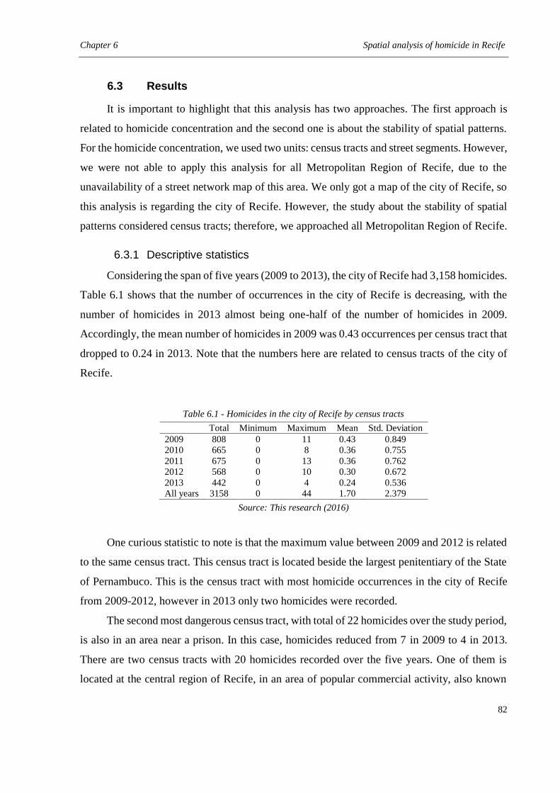
Chapter 6 Spatial analysis of homicide in Recife
82
6.3 Results
It is important to highlight that this analysis has two approaches. The first approach is
related to homicide concentration and the second one is about the stability of spatial patterns.
For the homicide concentration, we used two units: census tracts and street segments. However,
we were not able to apply this analysis for all Metropolitan Region of Recife, due to the
unavailability of a street network map of this area. We only got a map of the city of Recife, so
this analysis is regarding the city of Recife. However, the study about the stability of spatial
patterns considered census tracts; therefore, we approached all Metropolitan Region of Recife.
6.3.1 Descriptive statistics
Considering the span of five years (2009 to 2013), the city of Recife had 3,158 homicides.
Table 6.1 shows that the number of occurrences in the city of Recife is decreasing, with the
number of homicides in 2013 almost being one-half of the number of homicides in 2009.
Accordingly, the mean number of homicides in 2009 was 0.43 occurrences per census tract that
dropped to 0.24 in 2013. Note that the numbers here are related to census tracts of the city of
Recife.
Table 6.1 - Homicides in the city of Recife by census tracts
Total Minimum Maximum Mean Std. Deviation
2009 808 0 11 0.43 0.849
2010 665 0 8 0.36 0.755
2011 675 0 13 0.36 0.762
2012 568 0 10 0.30 0.672
2013 442 0 4 0.24 0.536
All years 3158 0 44 1.70 2.379
Source: This research (2016)
One curious statistic to note is that the maximum value between 2009 and 2012 is related
to the same census tract. This census tract is located beside the largest penitentiary of the State
of Pernambuco. This is the census tract with most homicide occurrences in the city of Recife
from 2009-2012, however in 2013 only two homicides were recorded.
The second most dangerous census tract, with total of 22 homicides over the study period,
is also in an area near a prison. In this case, homicides reduced from 7 in 2009 to 4 in 2013.
There are two census tracts with 20 homicides recorded over the five years. One of them is
located at the central region of Recife, in an area of popular commercial activity, also known
Chapter 6 Spatial analysis of homicide in Recife
83
for prostitution, drugs and low income. The other census tract is a residential area, marked by
a lack of infrastructure and low income. In the first census tract no homicides were registered
in 2013 and in the second census tract, only one homicide occurred in 2013.
Analyzing the areas with the greatest volume of homicides between 2009 and 2013, we
can suggest that changes have occurred. Those areas had a disproportionate number of
homicides relative to other areas of the city in 2009, but these numbers were disproportionately
reduced by 2013, consistent with the crime and place literature. Beyond these examples, we can
highlight that 17 census tracts in Recife had a homicide drop greater than 3 occurrences between
2009 and 2013. However, the city of Recife also experienced an increase on homicides in some
areas. These census tracts are generally composed of high vulnerability areas.
In addition to this descriptive account, Figure 6.1 shows the number of census tracts in
the city of Recife by the count of homicides for each year. Based on Figure 6.1, we can see that
the percentage of census tracts with no homicide occurrences has increased. This is a somewhat
expected result because the number of homicides dropped in the city of Recife during this
period. In addition, the volume of homicides within census tracts also decreased: in 2009, the
maximum value was 11, while this number was 4 in 2013.
Figure 6.1 - Histograms of number of homicides per census tract in the city of Recife
Source: This research (2016)
Figure 6.1 suggests that there is a concentration of homicides in the city of Recife, because
the great majority of census tracts do not have any occurrences. At the same time, however, the
0
200
400
600
800
1000
1200
1400
1600
2009 2010 2011 2012 2013
0
1
2
3
4
5 or more
Chapter 6 Spatial analysis of homicide in Recife
84
graphs reveal that there is no evidence for concentrations within the concentrations because
there is not a high frequency of homicides in any given census tract. Nevertheless, this topic
will be discussed further below.
Considering street segments, two locations had more than ten homicides between 2009
and 2013. These streets are cross streets and located beside the biggest prison of Pernambuco.
Incidentally, this shows the importance of the scale of analysis because it illustrates how two
street segments (one intersection) can drive the results for an entire census tract.
Other street segments had between 5 and 10 homicides during the five years and they are
located in vulnerable or low-income areas. Some of these places are areas with high levels of
social interaction, near city squares and bars. One of the street segments is located in a wealthy
neighborhood, beside a shopping center. However, this adjacent area is a slum, characterized
by low levels of infrastructure and income. This example highlights the significant
socioeconomic disparities that can be found in Recife.
6.3.2 Homicide concentrations
In order to answer the first research question and test the corresponding hypothesis, Table
6.2 shows the degree of spatial concentration at census tract and street segment levels. The first
column shows that the percentage of census tracts with any homicides has been decreasing,
2009 - 2013: 29 to 19 percent. As such, many of Recife’s census tracts are free of homicides.
Given the high levels and rates of homicides in this city, such a result is interesting on its own.
Table 6.2 - Percentages of homicides in the city of Recife
Year Percent of census tracts
with homicides
Percent of census tracts with homicides
that account for 50 percent of homicides
2009 29.13 28.52
2010 25.35 29.36
2011 26.21 30.86
2012 23.25 34.57
2013 19.36 39.00
Year Percent of street segments
with homicides
Percent of street segments with homicides
that account for 50 percent of homicides
2009 2.32 45.24
2010 1.93 45.93
2011 1.95 45.72
2012 1.68 47.19
2013 1.30 46.73
Source: This research (2016)
Chapter 6 Spatial analysis of homicide in Recife
85
The second column shows that the percentage of census tracts with any homicides that
account for 50 percent of homicides has been increasing: 29 to 39 percent. Any percentage here
that is substantially less than 50 percent indicates a hot spot within a hot spot because of the
concentration of homicides at the census tract level, as a whole. However, what has been
occurring in the city of Recife is that homicides are occurring within fewer census tracts, but
the distribution of those remaining homicides has become more dispersed.
Measuring homicides at the street segment level shows a far greater concentration of
homicide. Though just almost 10 percent of street segments had at least one homicide over the
five-year period, in any given year just 2.3 percent or less of the street segments had one or
more homicides. In fact, there has been a steady decrease in the percentage of street segments
that had any homicides: 2.32 to 1.3 percent. This is an incredible spatial concentration,
particularly at the street segment level. Most often in the crime and place research, 5 percent of
street segments (micro-places) are able to account for 50 percent of crimes (Weisburd & Arman,
2014). However, in the current analysis less than 2 percent of street segments can account for
all homicides in the city of Recife (2010-2013). Of course, homicide is a much rarer criminal
event than most of the crime types investigated in the crime and place literature (assault,
burglary, robbery, etc.), but this is a notably high degree of crime concentration. Therefore, we
confirmed our first hypothesis that the law of crime concentration at places holds for homicide
in the city of Recife.
Because of this high concentration of homicides, it should come as no surprise that
almost 50 percent of street segments with any homicides are needed to account for 50 percent
of homicides in the city of Recife. Of particular note here, however, is that this last percentage
has been stable during the drop in homicide rates. This result, in conjunction with the fact that
the percentage of street segments with any homicides has decreased, gives an indication that
the spatial pattern of homicide has changed during this time period. As such, we may reject our
second hypothesis. Moreover, we can say that homicides are well dispersed within the street
segments – there are no hotspots inside the hotspots.
6.3.3 Stability of spatial concentrations
Firstly, we investigate the stability of the spatial patterns along the years. Therefore, we
analyzed the spatial pattern year by year and the S-indices are shown in Table 6.3. It is important
to notice that these analyses were made considering all Metropolitan Region of Recife because
Chapter 6 Spatial analysis of homicide in Recife
86
the street segment level is not necessary anymore. The SPPT was employed on all spatial units
available as well as only those spatial units within which homicides occurred. This was done as
a sensitivity analysis for the stability of homicides because there are many spatial units of
analysis that have zero values in all years (Andresen & Malleson, 2011).
Table 6.3 - Results of spatial point pattern test by year
2009-2010 2009-2011 2009-2012 2009-2013
All census tracts (4,589) 0.7494 0.7496 0.7468 0.7424
Census tracts with homicides (3,004) 0.6175 0.6192 0.6119 0.6065
Source: This research (2016)
In Table 6.3, we can note that the values of all census tracts are higher than the values of
only census tracts with occurrences. This confirms that the issue regarding the S-Index inflation
referred by Andresen & Malleson (2011) is present in this analysis too. When the spatial point
pattern test with all census tracts is applied, 1,585 areas are inflating S-Index with their zero
homicides (consequently, no variance and indicating similarity). For the five years under
analysis, homicides only occurred in just over 65 percent of the census tracts in Recife, 3,004
of 4,589 census tracts. Due to this fact, we opted to consider the census tracts with occurrences.
Observing the results of the SPPT only using census tracts that had at least one homicide
in any of the years under analysis, we see that the S-Indices have a level that cannot be
considered similar, at or just above 0.62. Essentially, all the values are between 0.60 and 0.62,
indicating that the spatial pattern of homicides at the census tract level was similar for 60-62
percent of the census tracts in Recife, comparing 2009 to the other available years – similar
results are present when comparing other year combinations. This indicates that over time there
has been a major spatial shift in the pattern of homicides in Recife as it has experienced a
significant drop in this crime type. This does not support our second hypothesis.
The results of the spatial point pattern test, therefore, give a clear result for the second
hypothesis: the spatial patterns of homicide are not stable over time. Moreover, we can
hypothesize about this finding: in a span of five years, perhaps, the local dynamic can
experienced some changes – different interaction areas, drug points, and bars for example.
However, as we mentioned in Chapter 5, the annual aggregation of homicide is not
recommended when spatial patterns matter. In this way, we performed the SPPT respecting the
temporal dimensions, in order to verify the stability of spatial patterns along the years. Because
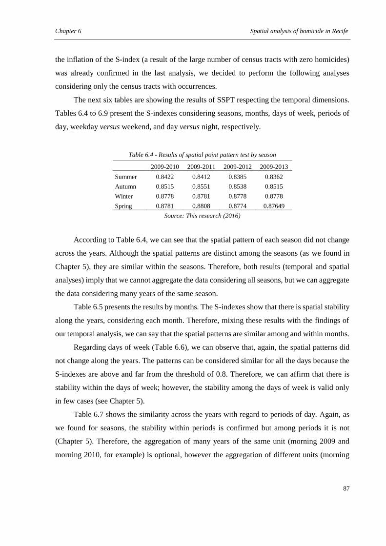
Chapter 6 Spatial analysis of homicide in Recife
87
the inflation of the S-index (a result of the large number of census tracts with zero homicides)
was already confirmed in the last analysis, we decided to perform the following analyses
considering only the census tracts with occurrences.
The next six tables are showing the results of SSPT respecting the temporal dimensions.
Tables 6.4 to 6.9 present the S-indexes considering seasons, months, days of week, periods of
day, weekday versus weekend, and day versus night, respectively.
Table 6.4 - Results of spatial point pattern test by season
2009-2010 2009-2011 2009-2012 2009-2013
Summer 0.8422 0.8412 0.8385 0.8362
Autumn 0.8515 0.8551 0.8538 0.8515
Winter 0.8778 0.8781 0.8778 0.8778
Spring 0.8781 0.8808 0.8774 0.87649
Source: This research (2016)
According to Table 6.4, we can see that the spatial pattern of each season did not change
across the years. Although the spatial patterns are distinct among the seasons (as we found in
Chapter 5), they are similar within the seasons. Therefore, both results (temporal and spatial
analyses) imply that we cannot aggregate the data considering all seasons, but we can aggregate
the data considering many years of the same season.
Table 6.5 presents the results by months. The S-indexes show that there is spatial stability
along the years, considering each month. Therefore, mixing these results with the findings of
our temporal analysis, we can say that the spatial patterns are similar among and within months.
Regarding days of week (Table 6.6), we can observe that, again, the spatial patterns did
not change along the years. The patterns can be considered similar for all the days because the
S-indexes are above and far from the threshold of 0.8. Therefore, we can affirm that there is
stability within the days of week; however, the stability among the days of week is valid only
in few cases (see Chapter 5).
Table 6.7 shows the similarity across the years with regard to periods of day. Again, as
we found for seasons, the stability within periods is confirmed but among periods it is not
(Chapter 5). Therefore, the aggregation of many years of the same unit (morning 2009 and
morning 2010, for example) is optional, however the aggregation of different units (morning
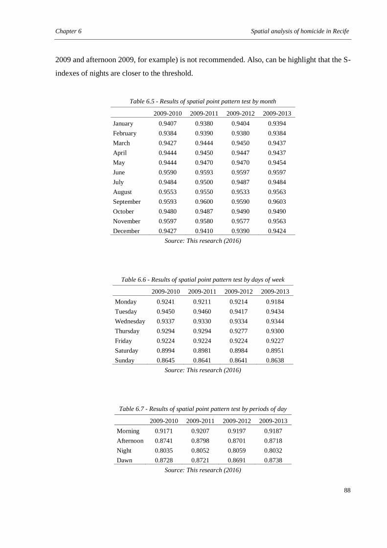
Chapter 6 Spatial analysis of homicide in Recife
88
2009 and afternoon 2009, for example) is not recommended. Also, can be highlight that the S-
indexes of nights are closer to the threshold.
Table 6.5 - Results of spatial point pattern test by month
2009-2010 2009-2011 2009-2012 2009-2013
January 0.9407 0.9380 0.9404 0.9394
February 0.9384 0.9390 0.9380 0.9384
March 0.9427 0.9444 0.9450 0.9437
April 0.9444 0.9450 0.9447 0.9437
May 0.9444 0.9470 0.9470 0.9454
June 0.9590 0.9593 0.9597 0.9597
July 0.9484 0.9500 0.9487 0.9484
August 0.9553 0.9550 0.9533 0.9563
September 0.9593 0.9600 0.9590 0.9603
October 0.9480 0.9487 0.9490 0.9490
November 0.9597 0.9580 0.9577 0.9563
December 0.9427 0.9410 0.9390 0.9424
Source: This research (2016)
Table 6.6 - Results of spatial point pattern test by days of week
2009-2010 2009-2011 2009-2012 2009-2013
Monday 0.9241 0.9211 0.9214 0.9184
Tuesday 0.9450 0.9460 0.9417 0.9434
Wednesday 0.9337 0.9330 0.9334 0.9344
Thursday 0.9294 0.9294 0.9277 0.9300
Friday 0.9224 0.9224 0.9224 0.9227
Saturday 0.8994 0.8981 0.8984 0.8951
Sunday 0.8645 0.8641 0.8641 0.8638
Source: This research (2016)
Table 6.7 - Results of spatial point pattern test by periods of day
2009-2010 2009-2011 2009-2012 2009-2013
Morning 0.9171 0.9207 0.9197 0.9187
Afternoon 0.8741 0.8798 0.8701 0.8718
Night 0.8035 0.8052 0.8059 0.8032
Dawn 0.8728 0.8721 0.8691 0.8738
Source: This research (2016)
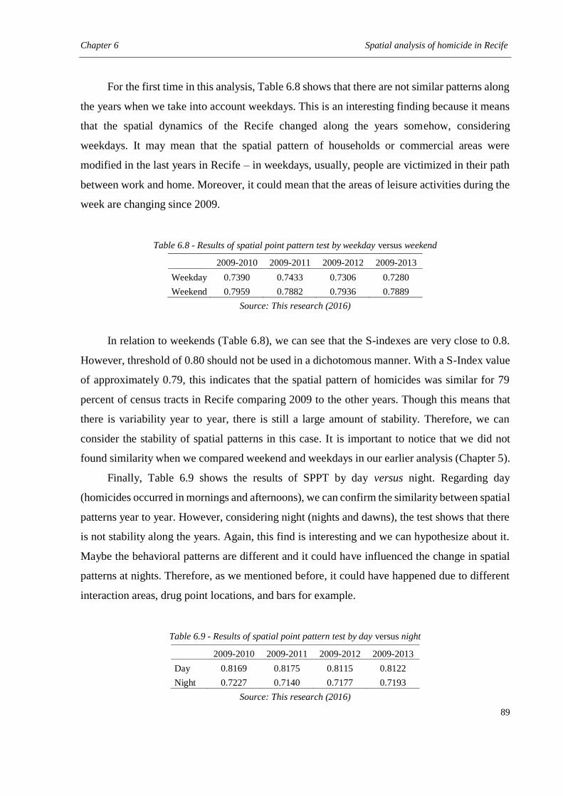
Chapter 6 Spatial analysis of homicide in Recife
89
For the first time in this analysis, Table 6.8 shows that there are not similar patterns along
the years when we take into account weekdays. This is an interesting finding because it means
that the spatial dynamics of the Recife changed along the years somehow, considering
weekdays. It may mean that the spatial pattern of households or commercial areas were
modified in the last years in Recife – in weekdays, usually, people are victimized in their path
between work and home. Moreover, it could mean that the areas of leisure activities during the
week are changing since 2009.
Table 6.8 - Results of spatial point pattern test by weekday versus weekend
2009-2010 2009-2011 2009-2012 2009-2013
Weekday 0.7390 0.7433 0.7306 0.7280
Weekend 0.7959 0.7882 0.7936 0.7889
Source: This research (2016)
In relation to weekends (Table 6.8), we can see that the S-indexes are very close to 0.8.
However, threshold of 0.80 should not be used in a dichotomous manner. With a S-Index value
of approximately 0.79, this indicates that the spatial pattern of homicides was similar for 79
percent of census tracts in Recife comparing 2009 to the other years. Though this means that
there is variability year to year, there is still a large amount of stability. Therefore, we can
consider the stability of spatial patterns in this case. It is important to notice that we did not
found similarity when we compared weekend and weekdays in our earlier analysis (Chapter 5).
Finally, Table 6.9 shows the results of SPPT by day versus night. Regarding day
(homicides occurred in mornings and afternoons), we can confirm the similarity between spatial
patterns year to year. However, considering night (nights and dawns), the test shows that there
is not stability along the years. Again, this find is interesting and we can hypothesize about it.
Maybe the behavioral patterns are different and it could have influenced the change in spatial
patterns at nights. Therefore, as we mentioned before, it could have happened due to different
interaction areas, drug point locations, and bars for example.
Table 6.9 - Results of spatial point pattern test by day versus night
2009-2010 2009-2011 2009-2012 2009-2013
Day 0.8169 0.8175 0.8115 0.8122
Night 0.7227 0.7140 0.7177 0.7193
Source: This research (2016)
Chapter 6 Spatial analysis of homicide in Recife
90
6.4 Discussion
In this analysis, we have investigated the crime concentrations and the changing of spatial
patterns of homicide in Recife, specifically in the context of the homicide drop in recent years.
We found that there is a high degree of concentration in homicide in the city of Recife. As noted
above, in any given year homicides only occur on 1.30 to 2.32 percent of street segments. In
the case of 2009 (2.32 percent) this still represents over 700 street segments in the city of Recife
that have homicides – just over 400 in 2013. Overall, we found strong support for our first
hypothesis that the law of crime concentrations at places applies to homicide in the city of
Recife, and we have support to reject our second hypothesis that these spatial patterns are stable
over time.
In the city of Recife, homicides decreased by 44.75 percent from 2009 – 2013. The
reduction in the percentage of street segments with homicides (2.32 to 1.30 percent) is a 44
percent drop. Moreover, the percentage of street segments needed to account for 50 percent of
homicides remains unchanged over the study period. Collectively, these results imply that
homicides have decreased at approximately the same degree as the concentration of homicides
at the street segment level has increased, with the density of homicides remaining the same. If
homicides had decreased everywhere by the same degree indicating a more general decrease in
violence, we would not expect these two numbers to change in this way. Rather, the percentage
of street segments with homicides would also remain relatively stable over time with fewer
homicides per street segment. This implies that just over 40 percent of the street segments that
had homicides in 2009 no longer had homicides in 2013, and we know that this included some
of the highest volume street segments in the city.
Though we do not conduct trajectory analyses to investigate the stability of spatial
homicide patterns, the results are best compared with this research. Weisburd et al. (2004)
found that 84 percent of the street segments in Seattle, Washington (1989 – 2002) had stable
trajectories over their study period. In the context of the crime drop that occurred in Seattle, a
24 percent decrease in crime over the study period, 14 percent of the street segments had
decreasing crime trends. Through the use of growth curve analysis, Braga et al. (2010; 2011)
found similar results in the context of robberies in Boston, Massachusetts (1980 – 2008).
Specifically, the concentrations of robbery are relatively stable over time and, consequently, a
small percentage of street segments and intersections accounted for the majority of the crime
drop.
Chapter 6 Spatial analysis of homicide in Recife
91
Most recently, Curman et al (2015) used the same trajectory analysis method as Weisburd
et al. (2004) and found that 70 percent of the street segments in Vancouver, British Columbia
(1991 – 2006) had stable trajectories, with the crime drop (a 40 percent decline) being driven
by 30 percent of the street segments in the city – these numbers are in line with our street
segment results, reported above. However, using a different trajectory analysis method, Curman
et al. (2015) found that 94 percent of the street segments had stable trajectories, with 6 percent
of the street segments being the driving force of the crime drop in Vancouver. Overall, this
research has found that criminal opportunities are largely stable over time and that a relatively
small percentage of street segments have exhibited the greatest drops in criminal activity. These
results imply that crime prevention activities that are place-based have the greatest promise for
dealing with criminal activity (Braga et al., 2010; Braga et al., 2011).
In the context of homicide in the city of Recife, the results exhibit a similar pattern when
considering census tracts. With a reduction in homicides of over 40 percent and homicides
occurring in so few places within the city, something must have occurred at very specific places
rather than citywide initiatives. Moreover, the decrease in homicides had a particular pattern:
fewer census tracts currently experience homicides and the distribution of homicides has
become more even. This result implies that the relatively small percentage of census tracts that
had high volumes of homicides experienced the greatest drops. If the drop in homicides was
uniform across all places, the percentage of census tracts that account for 50 percent of
homicides would have remained low, showing a concentration within a concentration.
However, this percentage of census tracts increased (see Table 6.2), indicating the greatest
volume census tracts had the greatest decreases.
Though the same result was found for the street segments in the context of a decreasing
percentage of street segments with any homicides, the degree of uniformity across those street
segments has essentially remained unchanged – a uniform distribution of homicides from 2009
– 2013. However, recall from the discussion above there are street segments with
disproportionately high volumes of homicide in the city of Recife that also had the largest drops.
Though these drops in homicide were not enough to manifest themselves in the citywide
statistics, they do occur, supporting the placed-based crime prevention activities put forth by
Weisburd et al. (2004) and Braga et al. (2010, 2011).
At this stage of the research, placed-based crime prevention activities are hypotheses
that need to be tested, but the necessary data are not available to me for any such hypothesis
Chapter 6 Spatial analysis of homicide in Recife
92
testing. In the context of the international crime drop, explanations for this phenomenon are
unsatisfactory, particularly for violent crime (Farrell, 2013). However, there has been a crime
prevention initiative in Pernambuco that has been implicated for being responsible for the
homicide decline. The Pact for Life Program was explained before in Section 4.5. Though
circumstantial without any scientific evaluations to date, Pact for Life is a promising
explanation given that homicide for Brazil, as a whole, increased after 2007.
The results of this analysis look promising and can guide future research in this area.
Primarily, in the current context, future research should be conducted through evaluations of
plausible rival hypotheses for the drop in homicide in Recife, Brazil. Though there is research
investigating the Pact for Life, proper evaluations must be undertaken. The programs that are
then found to be effective can be replicated elsewhere in Brazil and other places in which
homicide is an issue. There are many street segments that have exhibited decreases (complete
reductions, specifically) of homicide in Recife, so these street segments must be identified and
compared to the locations in which the Pact for Life projects have been implemented. If the
PFL projects have a greater presence in the location in which homicides have decreased, then
we would be one step closer to identifying changes that impact the occurrence of homicide.
Additionally, there are likely Pact for Life projects that have a greater effect on homicide
than others than can be identified in such an analysis. For example, the longer term projects
(primary prevention) may not have had a chance to impact homicide yet, and there may be
secondary and/or tertiary projects that have more or less success in particular places. And more
generally, the crime drop is an international phenomenon that should be studied further at the
micro-spatial scale. Only through the replication of these, and other, results can we confidently
proceed with place-based crime prevention activities.
Such future research is important not only for the well-being of Recife, but also for other
locations that have a high degree of violence. Though we are moving toward a better
understanding of the forces behind the international drop in property crime, namely opportunity,
the corresponding international drops in violent crime are less understood (Farrell et al., 2014).
Because of the high volume of homicides, places in countries like Brazil provide an opportunity
to better understand criminological events that are relatively rare in many countries. As a
consequence, we may be able to learn more about these phenomena in order to prevent them.
Chapter 6 Spatial analysis of homicide in Recife
93
6.5 Final comments
The spatial analysis was aimed to investigate the homicide concentration and the spatial
stability of homicides in Recife. Regarding the homicide concentration, we found that
homicides are very concentrated in the city of Recife. All the homicides between 2009 and 2013
occurred in less than 10 percent of the street segments of this city. Even though homicides are
a rare event, this is a notably high degree of crime concentration.
Moreover, we employed the spatial point pattern test in order to verify the stability of
homicide spatial patterns along the years. The S-indexes showed that the patterns were not
stable from 2009 to 2013. However, according to the findings of Chapter 5, is not appropriate
to analyze homicides by year when spatiality is important. In this sense, we checked the stability
along the years considering six spatial dimensions. SPPT test revealed that the patterns were
stable along the years when we took into account the spatial dimensions – except for weekdays
and night/dawn. Therefore, it suggests that the behavioral patterns are different and it could
have influenced the change in spatial patterns at weekends and nights.
Chapter 7 Environmental analysis of homicide in Recife
94
7 ENVIRONMENTAL ANALYSIS OF HOMICIDE IN RECIFE
In this analysis, we investigate which environmental factors are related to homicides in
Recife, considering social disorganization theory. In this way, we used social, economic, and
demographic variables from 2010 demographic census. Using geo-referenced homicide data
(2009 to 2013) and census data, we analyzed homicide in Recife using a spatial regression
technique that controls for spatial autocorrelation and heteroskedasticity.
Positive significant relationships were found for inequality, rented houses and quantity of
people, but negative relationships for income, literacy, public illumination, street network
density, and population density. Overall, we conclude that social disorganization theory
provides an instructive framework for understanding homicide in Recife. However, there are
specific contexts to Brazil that are different from North American contexts.
7.1 Contextualization
Historically, Brazil has been marked by violence, emphasizing the colonization process,
the slave market, and the military dictatorship (Oliveira Júnior, 2013). Currently, violence is
primarily understood through drug trafficking and disputes between criminal factions.
Moreover, this unfavorable context is aggravated by unemployment, inequality, and low
education. A research published by IPEA reveals that the Brazilian population thinks that the
causes of criminality in Brazil are social and economic inequality and a lack of investment in
education (IPEA, 2012).
In the context of the state of Pernambuco, Lima et al. (2002) attributed violence to high
illiteracy rates, unemployment, high-income concentration, and social inequality. This situation
developed an atmosphere that was conducive to violence and the consequences continue today.
Although Pernambuco experienced an increase in its socio-economic indicators in the recent
years, the homicide rate is still significantly higher than the national average.
Specifically with regard to the Metropolitan Region of Recife, Lima et al. (2005a)
highlighted the context of drugs, interpersonal conflict, and the formation of gangs. Minayo &
Constantino (2012) conducted a qualitative research in one of the municipalities of MRR and
the respondents believe that violence is related to drug trafficking, with an emphasis on
grooming youth, and the conflicts between traffickers and users.
Chapter 7 Environmental analysis of homicide in Recife
95
Many works were written about the determinants of criminality, as we showed in Chapter
3. This kind of study is important because it can show which factors contribute to the criminal
activity and then we can have a better understanding about the topic. When we know the
elements that influence a problem, we can treat it in a more efficient manner. This study
investigates the determinants of homicides in Recife, taking into account social disorganization
theory. This theory (we discussed about that in Chapter 3) is quite widespread and defends that
criminality is related to neighborhood ecological characteristics.
7.2 Purpose of environmental analysis
The environmental analysis aims to respond the question: which environmental factors
are related to homicides in Recife? Therefore, this study investigates the role of demographic,
social, and economic variables that may be associated with homicides. The variables were
chosen considering the social disorganization theory. We consider ethnic heterogeneity, social
and economic deprivation, family disruption, population turnover, employment status,
population characteristics, and income levels as factors related to social disorganization theory.
It is important to notice that some peculiar variables were considered in this analysis, in order
to incorporate the specifics of Brazilian context.
To answer this question, we used spatial regression. The analysis was made within
Metropolitan Region of Recife, taking into account census tracts. We expected a statistically
significant relation of homicides with inequality and education, as pointed out by the research
of IPEA.
This analysis differentiates itself from the other works in three ways: (1) we used a spatial
regression technique that controls for spatial autocorrelation and heteroscedasticity; (2) we
considered an expanded set of potential explanatory variables: 29 variables, in total; and (3) we
include unusual variables in order to incorporate the specifics of Brazilian context.
7.3 Environmental variables
Our selection of explanatory variables is dominantly based on social disorganization
theory. Based on the literature review, we considered the theory in general as well as specifics
in Brazil. We took into account seven factors related to social disorganization theory (ethnic
heterogeneity, social and economic deprivation, family disruption, population turnover,
Chapter 7 Environmental analysis of homicide in Recife
96
employment status, population characteristics, and income levels) and we chose 29 variables
related to them.
In the context of social disorganization theory more generally, Shaw & McKay (1942)
found that the two primary aspects of a neighborhood that lead to social disorganization are
population turnover and ethnic heterogeneity. With greater levels of population turnover
(usually because of poor economic conditions), fewer people were able to establish a local
network that allowed for setting common goals to reduce criminal activity. Ethnic heterogeneity
also contributed to this inability of a neighborhood to come together, primarily because people
literally could not understand one another: ethnic heterogeneity at that time in Chicago meant
that people came from different countries (most often European countries) and did not share a
common language.
In their causal model of social disorganization theory, Sampson & Groves (1989)
expanded on the work of Shaw & McKay in the following way: sparse local friendship
networks, unsupervised teenage peer groups, and low organizational (neighborhood)
participation led to crime and delinquency. These three factors were influenced by low
economic status, ethnic heterogeneity, residential mobility, family disruption, and urbanization.
These five factors have been measured in a number of different ways, most often using census
data in the geography of crime literature. Therefore, in this study, we chose the environmental
factors taking into account the works of Shaw & McKay (1942) and Sampson & Groves (1989).
In order to measure ethnic heterogeneity, we used Blau's heterogeneity index (Blau,
1977). This index can be calculated according to Equation (7.1):
1 − ∑ 𝑝𝑖2
𝑖 (7.1)
where pi is the proportion of members in the ith category. When the group is totally
homogeneous this index is 0. The maximum value, however, will depend on the number of
categories. The maximum value is given by (k-1)/k, where k is the number of categories. In
Recife, the ethnic heterogeneity related to nationality is quite weak. People from different
nationalities are not common in Recife, but the racial heterogeneity is strong across the entire
country. Because of this, in this study, we considered heterogeneity as the difference among
races. In our case, the demographic census takes into account six categories for race (White,
Black, Asian, South Asian, Indigenous, and “Other”), so the maximum value for Blau's index
is 0.833.
Chapter 7 Environmental analysis of homicide in Recife
97
Also in relation to ethnic heterogeneity, we considered black population. We included
two variables for the black population: the percentage of black people and the percentage of
black males between 15 and 24 years old. In the work of Breetzke (2010), the percentage of
blacks also was utilized to represent ethnic heterogeneity. It is important to note that the
presence of these sub-populations do not represent a particularly criminogenic group, but rather
social and historical conditions that are not easily represented with other socio-economic
variables.
We measure social and economic deprivation using variables representing education,
inequality and vulnerability. Regarding education, two variables are considered: literate people
older than 5 years old and literate people older than 15 years old. As mentioned above, research
on public opinion and research in general has identified inequality is an important factor to
understand the criminal activity. Though the Gini index is commonly used for a measure of
inequality in an area, this indicator is not available at census tract level. In its place, we use the
standard deviation of the monthly income of household heads and the Index of Concentration
at the Extremes (ICE).
The standard deviation of income shows the dispersion between people’s income. ICE
measures concentrations of wealth and poverty within a neighborhood or area, recognizing that
it is the “proportional imbalance between affluence and poverty within a neighborhood that
really matters” (Massey, 2001). The index can be calculated as the difference between the
number of families or persons classified as wealthy and the number of families or persons
classified as poor in a given neighborhood divided by the population of that neighborhood. ICE
can range between -1 and 1: -1 means that all families/persons are poor, 1 means that all of
them are wealthy, and 0 means that the number of poor and wealthy is balanced (Massey, 2001).
We considered that poor people are those who live at the poverty line or lower; that is, living
with less than half of the minimum wage per month or do not have any income. With respect
to wealthy people, we considered those who receive at least ten times minimum wage per
month.
Still with the intent to represent social and economic deprivation, few variables were
included to capture the vulnerability of households or neighborhoods that are not available in
censuses within developed contexts. We chose seven variables to consider this vulnerability, a
common problem in Brazil and Recife: households with electricity, households with garbage
collection, households with water supply, households with an exclusive bathroom, households
Chapter 7 Environmental analysis of homicide in Recife
98
without open sewage, households with paving, households with public illumination, and the
percentage of improvised households. Improvised households are those that are inappropriate
for housing, such as slums or homes inside commercial establishments. We decided to not
consider an index that could aggregate all these variables because individual variables may
affect homicide in a different manner.
We considered the percentage of homes headed by women as proxy for single parent
families. Breetzke (2010) used the same variable to represent family disruption in a South
African context. In addition, two variables were included to capture the stability (or lack
thereof) in the neighborhood (population turnover): rented households and owned or in
acquisition households.
About employment status, there is not a variable measuring employment or
unemployment at census tract level. However, we included a proxy for employment status that
involves people without income: people without monthly income.
We also considered variables representing population characteristics. We included the
number of residents, population density, and street network density. The population count was
included because Boivin (2013) has identified this as a better method than calculating crime
rates at the neighborhood level. In order to obtain population density, we calculated the area
within ArcGIS software and then divided the population by the area; we used a similar method
to calculate the total length of streets in a census tract, dividing by its total area.
The percentage of the population between the ages of 15 and 24 years old and the
percentage of males between the ages of 15 and 24 years old was included to control for this
most criminogenic subpopulation (Hirschi & Gottfredson, 1983; Boyd, 2000). It is important
to mention that homicide was the main cause of external death for youths in MRR in 2010
(51.82 percent for people between 15 and 19 years old, and 44.56 percent for 20-29 years old)
(DATASUS, 2015).
We included the percentage of married people, defined as those people living with
spouses or partners (different or the same sex). We considered this variable because married
people tend to spend more of their free time at home, resulting in lower levels of victimization
(Kennedy & Forde, 1990). Consequently, they are less likely to spend time outside in socially
disorganized areas, placing them at risk of criminal victimization, including homicide because
of the possibility of being involved in fights or going to bars.
Chapter 7 Environmental analysis of homicide in Recife
99
We used multiple variables when considering income levels: people with monthly income
less than the minimum wage, people with monthly income greater than ten times the minimum
wage, and the natural logarithm of the value of monthly income of household heads. It is
important to highlight that in 2010 the minimum wage in Brazil was R$ 510 per month,
approximately US$150, considering the current exchange rate.
Finally, we included a dummy variable to identify if the census tract is located in a rural
or urban space.
As we can see, sometimes we used more than one variable to measure the same factor.
Because of that, we expected a very high correlation between some explanatory variables but
we decided to include all of them in the initial model to test which ones would better explain
homicides in Recife. We found very high correlations among some variables (greater than 0.8)
but we consider both individual and joint significance testing to avoid removing relevant
variables and avoiding omitted variable bias.
7.4 Results and discussion
7.4.1 Descriptive results
The descriptive statistics for the dependent and independent variables are shown in Table
7.1. The dependent variable is the sum of homicides for 2009 to 2013 in order to prevent the
analysis of an aberrant year of data. As shown in Table 7.1, homicides range from 0 to 25 with
a mean of 2.14 homicides per census tract. Generally speaking, the table shows how the census
tracts of Metro Recife vary significantly in the context of homicide, as well as variables
representing social, economic, and demographic factors. The range of all variables indicates
that there is little evidence for homogeneity within the city, with only a few exceptions:
households with electricity, households with an exclusive bathroom, and urban space. These
results show the importance of using the smallest spatial unit as possible, with the intent of
capturing the particularities of each area.
Though the ranges of these variables are not often of principle interest in the spatial
criminology research, the context of a Brazilian city is particularly interesting. Regarding total
population, we can see that the range is large and, consequently, so is the standard deviation.
This can be explained by the agglomeration of residential buildings in Recife. The differences
of Recife’s population can be perceived by the large ranges for young population, young male
population, black population, young male black population, and married population. For
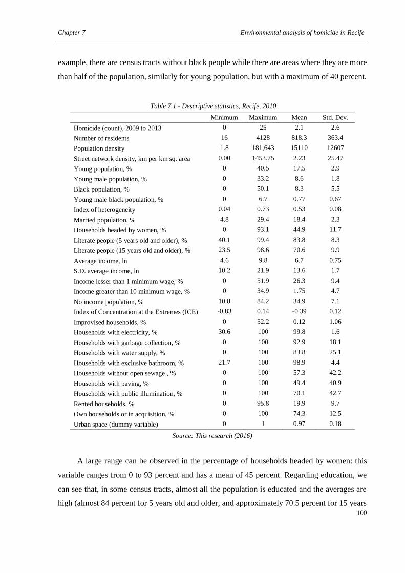
Chapter 7 Environmental analysis of homicide in Recife
100
example, there are census tracts without black people while there are areas where they are more
than half of the population, similarly for young population, but with a maximum of 40 percent.
Table 7.1 - Descriptive statistics, Recife, 2010
Minimum Maximum Mean Std. Dev.
Homicide (count), 2009 to 2013 0 25 2.1 2.6
Number of residents 16 4128 818.3 363.4
Population density 1.8 181,643 15110 12607
Street network density, km per km sq. area 0.00 1453.75 2.23 25.47
Young population, % 0 40.5 17.5 2.9
Young male population, % 0 33.2 8.6 1.8
Black population, % 0 50.1 8.3 5.5
Young male black population, % 0 6.7 0.77 0.67
Index of heterogeneity 0.04 0.73 0.53 0.08
Married population, % 4.8 29.4 18.4 2.3
Households headed by women, % 0 93.1 44.9 11.7
Literate people (5 years old and older), % 40.1 99.4 83.8 8.3
Literate people (15 years old and older), % 23.5 98.6 70.6 9.9
Average income, ln 4.6 9.8 6.7 0.75
S.D. average income, ln 10.2 21.9 13.6 1.7
Income lesser than 1 minimum wage, % 0 51.9 26.3 9.4
Income greater than 10 minimum wage, % 0 34.9 1.75 4.7
No income population, % 10.8 84.2 34.9 7.1
Index of Concentration at the Extremes (ICE) -0.83 0.14 -0.39 0.12
Improvised households, % 0 52.2 0.12 1.06
Households with electricity, % 30.6 100 99.8 1.6
Households with garbage collection, % 0 100 92.9 18.1
Households with water supply, % 0 100 83.8 25.1
Households with exclusive bathroom, % 21.7 100 98.9 4.4
Households without open sewage , % 0 100 57.3 42.2
Households with paving, % 0 100 49.4 40.9
Households with public illumination, % 0 100 70.1 42.7
Rented households, % 0 95.8 19.9 9.7
Own households or in acquisition, % 0 100 74.3 12.5
Urban space (dummy variable) 0 1 0.97 0.18
Source: This research (2016)
A large range can be observed in the percentage of households headed by women: this
variable ranges from 0 to 93 percent and has a mean of 45 percent. Regarding education, we
can see that, in some census tracts, almost all the population is educated and the averages are
high (almost 84 percent for 5 years old and older, and approximately 70.5 percent for 15 years
Chapter 7 Environmental analysis of homicide in Recife
101
old and older). However, we need to interpret these numbers with caution: for the demographic
census, a literate person is able to read and write a simple note. Therefore, being literate does
not indicate that the person has many years of education. Perhaps a better variable would be the
average of years of schooling, but this is not available in the census. Regarding the schooling
time, Pereira & Mota (2016) assert that few Human Development Units in Recife have
satisfactory mean years of schooling: the majority of the units do not achieve the period
mandated by Brazilian law.
Considering income, there is heterogeneity across census tracts. If we compare the
income among the census tracts (average income) and within census tracts (standard deviation
of average income), there are disparities/inequalities. Moreover, there are some areas where 50
percent of the people are living with less than the minimum wage ($150) per month, while in
other census tracts nobody lives in this situation. We also need to highlight that there are areas
where almost 85 percent of the population do not receive any income. In addition, the inequality
indicator has a maximum value of 0.99, confirming that there are extremely unequal areas in
Recife. Pereira & Mota (2016) indicate that many areas in Recife have monthly per capita
income lower than poverty line. According these authors, only 16.13 percent of the Human
Development Units in Recife could be classified as high or very high human development areas.
Finally, we considered the variables capturing the vulnerability of households and its
surroundings. These variables are of particular interest because they simply are not measured
in censuses in developed nations. Almost all the variables (aside from improvised households,
electricity, and exclusive bathroom) have a range between 0 and 100 percent, indicating
diversity within Recife: there are households and surroundings with basic infrastructure, but
there are entire neighborhoods (census tracts) that do not have this kind of service. However,
we can affirm that almost all the households have electricity and an exclusive bathroom, as
noted above. The variables that measure the quantity of rented and owned households also
present significant variation.
7.4.2 Inferential results
The results of the final spatial regression model are shown in Table 7.2 – the full model
with all explanatory variables is shown in Table 7.3. In the final model, the remaining
statistically significant variables are supportive of social disorganization theory. It should come
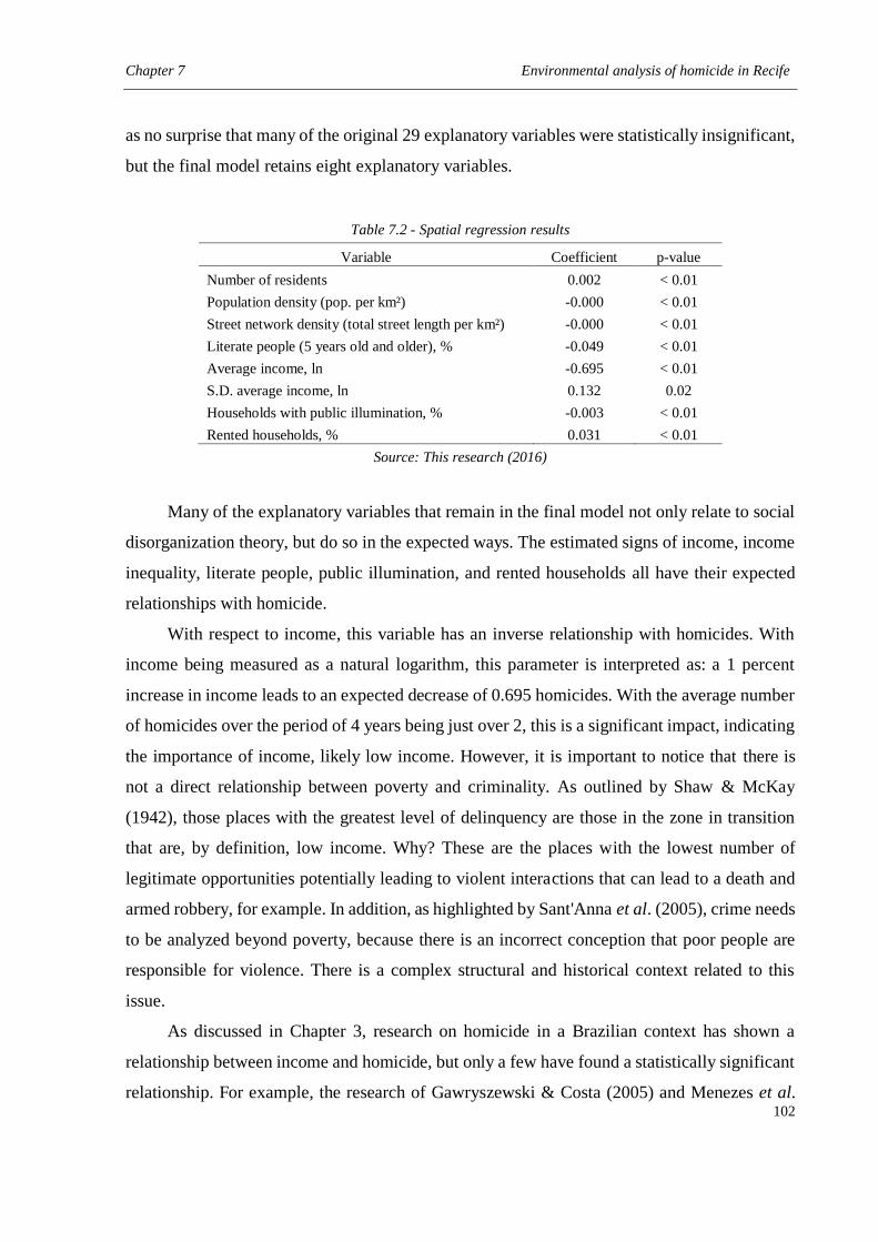
Chapter 7 Environmental analysis of homicide in Recife
102
as no surprise that many of the original 29 explanatory variables were statistically insignificant,
but the final model retains eight explanatory variables.
Table 7.2 - Spatial regression results
Variable Coefficient p-value
Number of residents 0.002 < 0.01
Population density (pop. per km²) -0.000 < 0.01
Street network density (total street length per km²) -0.000 < 0.01
Literate people (5 years old and older), % -0.049 < 0.01
Average income, ln -0.695 < 0.01
S.D. average income, ln 0.132 0.02
Households with public illumination, % -0.003 < 0.01
Rented households, % 0.031 < 0.01
Source: This research (2016)
Many of the explanatory variables that remain in the final model not only relate to social
disorganization theory, but do so in the expected ways. The estimated signs of income, income
inequality, literate people, public illumination, and rented households all have their expected
relationships with homicide.
With respect to income, this variable has an inverse relationship with homicides. With
income being measured as a natural logarithm, this parameter is interpreted as: a 1 percent
increase in income leads to an expected decrease of 0.695 homicides. With the average number
of homicides over the period of 4 years being just over 2, this is a significant impact, indicating
the importance of income, likely low income. However, it is important to notice that there is
not a direct relationship between poverty and criminality. As outlined by Shaw & McKay
(1942), those places with the greatest level of delinquency are those in the zone in transition
that are, by definition, low income. Why? These are the places with the lowest number of
legitimate opportunities potentially leading to violent interactions that can lead to a death and
armed robbery, for example. In addition, as highlighted by Sant'Anna et al. (2005), crime needs
to be analyzed beyond poverty, because there is an incorrect conception that poor people are
responsible for violence. There is a complex structural and historical context related to this
issue.
As discussed in Chapter 3, research on homicide in a Brazilian context has shown a
relationship between income and homicide, but only a few have found a statistically significant
relationship. For example, the research of Gawryszewski & Costa (2005) and Menezes et al.
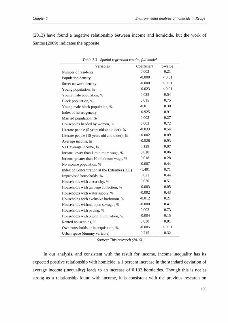
Chapter 7 Environmental analysis of homicide in Recife
103
(2013) have found a negative relationship between income and homicide, but the work of
Santos (2009) indicates the opposite.
Table 7.3 - Spatial regression results, full model
Variables Coefficient p-value
Number of residents 0.002 0.21
Population density -0.000 < 0.01
Street network density -0.000 < 0.01
Young population, % -0.023 < 0.01
Young male population, % 0.025 0.54
Black population, % 0.015 0.75
Young male black population, % -0.011 0.30
Index of heterogeneity -0.925 0.91
Married population, % 0.002 0.27
Households headed by women, % 0.003 0.72
Literate people (5 years old and older), % -0.033 0.54
Literate people (15 years old and older), % -0.002 0.09
Average income, ln -0.526 0.93
S.D. average income, ln 0.129 0.07
Income lesser than 1 minimum wage, % 0.010 0.06
Income greater than 10 minimum wage, % 0.018 0.28
No income population, % -0.007 0.44
Index of Concentration at the Extremes (ICE) -1.491 0.71
Improvised households, % 0.021 0.44
Households with electricity, % 0.030 0.51
Households with garbage collection, % -0.003 0.05
Households with water supply, % -0.002 0.43
Households with exclusive bathroom, % -0.012 0.21
Households without open sewage , % -0.000 0.41
Households with paving, % 0.002 0.73
Households with public illumination, % -0.004 0.15
Rented households, % 0.030 0.01
Own households or in acquisition, % -0.005 < 0.01
Urban space (dummy variable) 0.215 0.32
Source: This research (2016)
In our analysis, and consistent with the result for income, income inequality has its
expected positive relationship with homicide: a 1 percent increase in the standard deviation of
average income (inequality) leads to an increase of 0.132 homicides. Though this is not as
strong as a relationship found with income, it is consistent with the previous research on
Chapter 7 Environmental analysis of homicide in Recife
104
homicide in Brazil. However, there are other studies that have used the Gini Index, which is a
more direct measure (Araújo et al., 2010; Loureiro & Silva, 2012; Menezes at al., 2013;
Sachsida et al., 2007).
Literacy is found to have its expected inverse relationship with homicide. This is
consistent with the research of Santos (2009), but not Araújo et al. (2010) and Lima et al.
(2005b) who found a positive relationship. It is expected that positive relationships between
homicide and literacy are the result of omitted variable bias and/or rather aggregate spatial units
of analysis. Literacy is expected to lead to a decrease in homicide, and other criminal activity,
because a more literate population, on average, will be able to secure better employment and
greater income. Moreover, we can assume that school keeps the youths busy, lowering the
probability of their involvement in criminal activity. Consistent with this assumption, the work
of Sant'Anna et al. (2005) revels that 79 percent of the murdered youths in Porto Alegre (Brazil)
were not attending school when they were killed.
Public illumination was found to have a negative relationship with homicide. The
existence of public illumination can represent the presence of other infrastructure elements,
such as paving, sewage, or garbage collection. We can consider this variable as a measure for
social and economic deprivation, as well as the presence of public power. Moreover, we need
to take into account that public illumination can be a demotivating factor to commit murders in
such locales. Potential offenders may prefer to commit their crimes in dark public areas to avoid
the recognition and detection – see Farrington & Welsh (2002) for a systematic review of the
effects of street lighting on crime.
The percentage of rented houses has a positive relationship, as expected. This result is in
accordance with social disorganization theory because the greater the quantity of rented houses,
the greater is the turnover of the population. In areas with a high turnover, normally there is
little social and cultural cohesion that would bring a protective network to the neighborhood
because the population is not willing to make the effort to establish local connections.
Population density and street network density both have a negative impact in homicide.
There are two possible explanations for these results. First, considering the context of Recife,
we can confirm that population density is related to economic patterns. In Recife, some of the
wealthier neighborhoods contain large residential buildings, particularly those close to the
beach, that increase the density in these areas. These wealthier neighborhoods have fewer
homicides. As a second explanation, we can consider the theory of Jane Jacobs (1961): eyes on
Chapter 7 Environmental analysis of homicide in Recife
105
the street. Jacobs asserts that in areas with greater population density there is more traffic on
the streets. Therefore, such areas are less likely to experience criminal activities because the
aggressors believe that there is a greater probability of being seen or caught.
Finally, we can see that the number of residents is positively and significantly related to
the number of homicides, as expected: where there are more people, there are more potential
victims for homicides and crimes that may lead to a homicide, such as armed robbery. This
shows the importance of controlling for population size.
Overall, we can observe that social disorganization theory give insights about homicides
in Recife. The spatial regression results indicate that factors related to social disorganization
theory are important to understand the homicides in Recife. In the context of social
disorganization theory, it is important to note the work of Minayo & Constantino (2012) that
compares two Brazilian municipalities, one with high and other with low homicide rates.
According to these authors, some of the elements that distinguish both places are related to
social disorganization theory. In the less violent municipality, there are factors that contribute
positively with the social system and socialization of residents. In this area, “the social
relationships and the internal relations that promote social solidarity are internalized by the
culture”, with the presence of “communication network to promote the social control and the
cohesion among residents”, in addition to “there is more consensus, consistency and clarity
about the common values” (Minayo & Constantino, 2012). On the other hand, the violent
municipality is marked by the “dispersion of efforts” and “historical and persistent social
inequalities” that “reduced the collective effectiveness to face problems, creating a feeling of
withdrawal and impotence in relation to the criminality and the homicide is seen as an inevitable
fatality” (Minayo & Constantino, 2012). These authors also cite the example of three successful
programs to combat criminality in Brazil – the common point among them is the promotion of
social cohesion.
Considering the social disorganization theory and comparing with the factors pointed out
by Shaw & McKay (1942) and Sampson & Groves (1989), our results support the importance
of low economic status and residential mobility. Of particular interest to a lack of support is
ethnic heterogeneity. Recife has notable levels of ethnic heterogeneity (race), but none of the
variables representing this construct were statistically significant in any of the results.
The most direct measure of population turnover, rented households, supports the
hypothesis put forth in the social disorganization literature: more renters, more population, more
Chapter 7 Environmental analysis of homicide in Recife
106
homicides. Low economic status is also important but in particular ways. With regard to the
more traditional measure of economic status, the results here for income and income inequality
are supportive of the literature. But because of the magnitude of poverty not measured in
developed countries, low economic status was measured in Recife considering a host of other
neighborhood variables such as public illumination, electricity, and open sewers. One of these
variables proved to be statistically significant and in support of social disorganization theory.
As such, not only do we find expected relationships, consistent with the literature, but we also
find expected relationships that are consistent with the general concepts of social
disorganization theory and relate specifically to Brazil.
In relation to the correlation among the final model variables, we can say that only two
of the variables are very strongly correlated (greater than 0.8). The variables representing the
natural logarithm of average income and the natural logarithm of standard deviation of average
income present an almost perfect relationship among themselves (0.926). Because of this high
correlation, we performed tests removing these variables one at a time. When we removed either
average income or the standard deviation of average income the model results changed,
indicating omitted variable bias. This result, and the fact that both variables were statistically
significant in the final model, prompted us to keep both variables in the analysis despite their
high degree of correlation. Both variables are significant at the 5 percent level and although
there is an overlap between them, each one individually contributes to the model.
It is important to note that we also estimated count-data models. First, we estimated a
Poisson model and found similar results in comparison to the spatial regression model.
However, we did not opt for Poisson model because one assumption of this model was clearly
violated: the mean and the variance of the dependent variable are not equal (see Table 7.1).
Next, we considered the negative binomial model. The results were similar, but again changes
in the final model indicated bias, this time in standard errors. Specifically, more variables were
statistically significant in the final model. We opted to use the spatial regression because in the
presence of spatial autocorrelation, standard errors are underestimated potentially making
variables appear to be statistically significant when they are not. As such, because of the
similarity of the results with a negative binomial model, we chose to filter out spatial
autocorrelation and control for heteroskedasticity rather than run an explicit count-based model.
Chapter 7 Environmental analysis of homicide in Recife
107
7.5 Final comments
The environmental analysis revealed that homicide in Recife can be understood by social
disorganization theory. 29 explanatory variables were tested and eight of them were statistically
significant and consistent with the theory. We found that the variables related to inequality,
rented houses, and number of residents have a positive relationship with homicide. On the other
hand, income, education, public illumination, population density, and street network density
have a negative relationship.
Overall, income and inequality prove to be the most important variables for understanding
the distribution of homicide across the census tracts of Recife. This confirms previous research
as well as popular opinion in Brazil. However, our analysis extends previous research through
the extended set of explanatory variables, a priori, as well as a regression technique that
accounts for both spatial autocorrelation and heteroskedasticity.
Chapter 8 Identifying vulnerable areas to homicide in Recife
108
8 IDENTIFYING VULNERABLE AREAS TO HOMICIDE IN RECIFE
This chapter presents a preliminary attempt to identify vulnerable areas to homicide in
Metropolitan Region of Recife. We took into account the most relevant variables of our
environmental analysis to measure vulnerability for each census tracts. We employed
PROMETHEE II multicriteria method in order to aggregate the variables and we used local
Moran’s I to identify the most critical areas.
The result is a map highlighting two types of clusters and two outliers. The identification
of these areas is important because some actions may be directed to reduce vulnerability and,
consequently, decrease crime in long term. Because public resources are limited, some kind of
priority needs to be considered to allocate them. Therefore, this analysis suggests a structured
methodology to identify the most critical census tracts in RMR.
8.1 Contextualization
Violence is a problem in all world, mainly in developing nations. Countries like Brazil
have been trying to reduce their crime rates for many decades, with or without success. Brazil
is far from be an example in public security, even though many programs have been applied all
over the country. Therefore, there is a need of actions that are more efficient to combat and
prevent crimes. However, it is not only a question of which are the best actions, we also need
to define where the actions should be allocated.
Araújo Júnior & Fajzylber (2001) affirm that criminality is a social, economic, and
political problem that needs to be faced. It is social because it affects directly quality of life and
life expectancy. It is economic because it limits the economic development of a place. Finally,
it is political because the actions to deal with criminality involve a large participation of
governments and allocation of public resource.
It is impossible for a government improving police coverage, social conditions, or
economic factors in an entire city or state, for example. The resources to managing a place are
limited, so some kind of allocation have to be made, to direct the funds. For instance, Curtin et
al. (2005) assert that a good allocation of limited resources (considering police) may help in
reducing response time and saving money, without affect the level of attendance.
Therefore, the allocation of public resources is a relevant task. Due to this importance,
we need to guarantee the transparency and efficiency of the process. The opinion of a decision
Chapter 8 Identifying vulnerable areas to homicide in Recife
109
maker (mayor or manager, for instance) is crucial on this problem, but the decision process also
needs a formal methodology. The decision maker will contribute with his knowledge and
preferences, because he knows about the dynamics of the problematic. On the other hand, the
formal approach can help the expert to consider massive data or many viewpoints, for example.
Therefore, the junction of decision makers and structured models seems a good option to
allocate public resources.
Many works were written in this context, employing different techniques. Hirschfield &
Bowers (1997) developed a tool to analyze area profiles, showing applications in Merseyside
(England). These authors confirm that spatial variations of crime may be explained by several
factors as demographic, social, cultural, lifestyle, and land use characteristics. Due to this fact,
an approach involving more information can be more advantageous than hotspots considering
only past crimes. Therefore, they developed the software “profiler”, that is a demographic, land
use, and crime risk profiling system. Through this system, it is possible to address singular
insights, as the identification of disadvantaged areas and the effects of surroundings.
The paper of Caplan and colleagues (2011) shows the use of Risk Terrain Model to
forecast crimes of shooting. They assert that, usually, police agencies do crime analysis by
simple density maps, indicating a reactive attitude. However, an alternative would be to
consider factors that increase or decrease the propensity to crimes. Through Risk Terrain
Modeling, one is able to consider many factors to assess risk and the result is a map showing
the places with highest risk. They made an application in the community of Irvington (New
Jersey), considering dwellings of known gang members, locations of retail business
infrastructure, and locations of drug arrests. One of the conclusions of Caplan et al. (2011) is
that “the identification of risky areas permits public safety practitioners to intervene and allocate
resources to reduce risk”.
Gurgel & Mota (2013) also suggest a substitute approach to the police occurrences model:
a multicriteria method, SMARTS. Their procedure is aimed to suggest a structured
methodology to identify zones that are in greater need of public actions. They considered
population density, population growth, percentage of population living in bad conditions,
human development index, income concentration, and degree of police occurrences to order the
zones. An application was made in a Brazilian context and they concluded that their model can
be useful to public planning: “it may help to improve the management of public safety and to
reduce violence.”.
Chapter 8 Identifying vulnerable areas to homicide in Recife
110
A study was conducted by Camacho-Collados et al. (2015) with the objective of design
patrol sectors. They tried partitioning the territory in Madrid in the best possible way,
considering a multicriteria approach. The model includes the following attributes: area, support
received, demand, diameter, area ratio, isolation ratio, demand ratio, and diameter ratio. The
primary necessity of the model was to create districts as efficient and homogeneous as possible.
Camacho-Collados et al. (2015) affirm that their algorithm generates patrolling configurations
that are more efficient than the current one.
Recently, Bogomolov and colleagues (2015) published a study employing hotspot
classification, but considering additional information. They considered demographic factors
and people dynamics features, in order to identify places more or less likely to become crime
hotspots. The 124,119 small cells of London Metropolitan Area were classified as high or low
crime level in the next month (a dichotomic classification). The authors affirm that their model
has an accuracy of almost 70 percent, so the junction of aggregated and anonymized data
collected by the mobile infrastructure and demographic information seems to be useful to
evaluate crime levels. Bogomolov et al. (2015) affirms that their “proposed approach could
have clear practical implications by informing police departments and city governments on how
and where to invest their efforts and on how to react to criminal events with quicker response
times.”.
Figueiredo & Mota (2016) developed a Geographic Information System - Multicriteria
Decision Making model to evaluate security level in a Brazilian context. They applied
Dominance-Based Rough Set Approach to classify areas into five security levels, considering
income, Gini index, infrastructure, education, and demographic density. Figueiredo & Mota
(2016) affirms that this method does not require a high cognitive effort from the decision maker,
making the process easier.
We know that there are many papers written in this context, but these five examples
already show the concern of identifying most critical areas. Moreover, one can observe that this
evaluation should be made considering additional information, instead of only past occurrences.
This comprehensive approach to identify critical areas is valuable for public planning, because
it helps in the task of allocating resources. Therefore, this is the objective of this chapter.
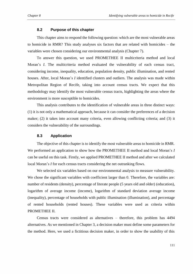
Chapter 8 Identifying vulnerable areas to homicide in Recife
111
8.2 Purpose of this chapter
This chapter aims to respond the following question: which are the most vulnerable areas
to homicide in RMR? This study analyses six factors that are related with homicides – the
variables were chosen considering our environmental analysis (Chapter 7).
To answer this question, we used PROMETHEE II multicriteria method and local
Moran’s I. The multicriteria method evaluated the vulnerability of each census tract,
considering income, inequality, education, population density, public illumination, and rented
houses. After, local Moran’s I identified clusters and outliers. The analysis was made within
Metropolitan Region of Recife, taking into account census tracts. We expect that this
methodology may identify the most vulnerable census tracts, highlighting the areas where the
environment is more susceptible to homicides.
This analysis contributes to the identification of vulnerable areas in three distinct ways:
(1) it is not only a mathematical approach, because it can consider the preferences of a decision
maker; (2) it takes into account many criteria, even allowing conflicting criteria; and (3) it
considers the vulnerability of the surroundings.
8.3 Application
The objective of this chapter is to identify the most vulnerable areas to homicide in RMR.
We performed an application to show how the PROMETHEE II method and local Moran’s I
can be useful on this task. Firstly, we applied PROMETHEE II method and after we calculated
local Moran’s I for each census tracts considering the net outranking flows.
We selected six variables based on our environmental analysis to measure vulnerability.
We chose the significant variables with coefficient larger than 0. Therefore, the variables are:
number of residents (density), percentage of literate people (5 years old and older) (education),
logarithm of average income (income), logarithm of standard deviation average income
(inequality), percentage of households with public illumination (illumination), and percentage
of rented households (rented houses). These variables were used as criteria within
PROMETHEE II.
Census tracts were considered as alternatives – therefore, this problem has 4494
alternatives. As we mentioned in Chapter 3, a decision maker must define some parameters for
the method. Here, we used a fictitious decision maker, in order to show the usability of this
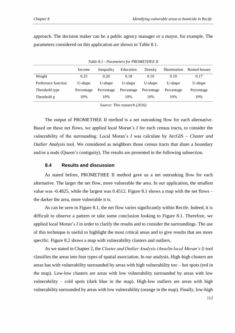
Chapter 8 Identifying vulnerable areas to homicide in Recife
112
approach. The decision maker can be a public agency manager or a mayor, for example. The
parameters considered on this application are shown in Table 8.1.
Table 8.1 - Parameters for PROMETHEE II
Income Inequality Education Density Illumination Rented houses
Weight 0.25 0.20 0.18 0.10 0.10 0.17
Preference function U-shape U-shape U-shape U-shape U-shape U-shape
Threshold type Percentage Percentage Percentage Percentage Percentage Percentage
Threshold 𝑞 10% 10% 10% 10% 10% 10%
Source: This research (2016)
The output of PROMETHEE II method is a net outranking flow for each alternative.
Based on these net flows, we applied local Moran’s I for each census tracts, to consider the
vulnerability of the surrounding. Local Moran’s I was calculate by ArcGIS – Cluster and
Outlier Analysis tool. We considered as neighbors those census tracts that share a boundary
and/or a node (Queen’s contiguity). The results are presented in the following subsection.
8.4 Results and discussion
As stated before, PROMETHEE II method gave us a net outranking flow for each
alternative. The larger the net flow, more vulnerable the area. In our application, the smallest
value was -0.4825, while the largest was 0.4512. Figure 8.1 shows a map with the net flows –
the darker the area, more vulnerable it is.
As can be seen in Figure 8.1, the net flow varies significantly within Recife. Indeed, it is
difficult to observe a pattern or take some conclusion looking to Figure 8.1. Therefore, we
applied local Moran’s I in order to clarify the results and to consider the surroundings. The use
of this technique is useful to highlight the most critical areas and to give results that are more
specific. Figure 8.2 shows a map with vulnerability clusters and outliers.
As we stated in Chapter 2, the Cluster and Outlier Analysis (Anselin local Moran’s I) tool
classifies the areas into four types of spatial association. In our analysis, High-high clusters are
areas has with vulnerability surrounded by areas with high vulnerability too – hot spots (red in
the map). Low-low clusters are areas with low vulnerability surrounded by areas with low
vulnerability – cold spots (dark blue in the map). High-low outliers are areas with high
vulnerability surrounded by areas with low vulnerability (orange in the map). Finally, low-high
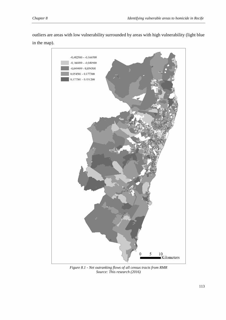
Chapter 8 Identifying vulnerable areas to homicide in Recife
113
outliers are areas with low vulnerability surrounded by areas with high vulnerability (light blue
in the map).
Figure 8.1 - Net outranking flows of all census tracts from RMR
Source: This research (2016)
Chapter 8 Identifying vulnerable areas to homicide in Recife
114
3754 census tracts were classified as not significant, 384 as high-high cluster, 312 as low-
low cluster, 13 as high-low outlier, and 31 as low-high outlier. Table 8.2 gives descriptive
statistics for each group and Figure 8.3 shows the boxplots (considering net outranking flows).
Figure 8.2 - Vulnerability clusters and outliers from RMR
Source: This research (2016)
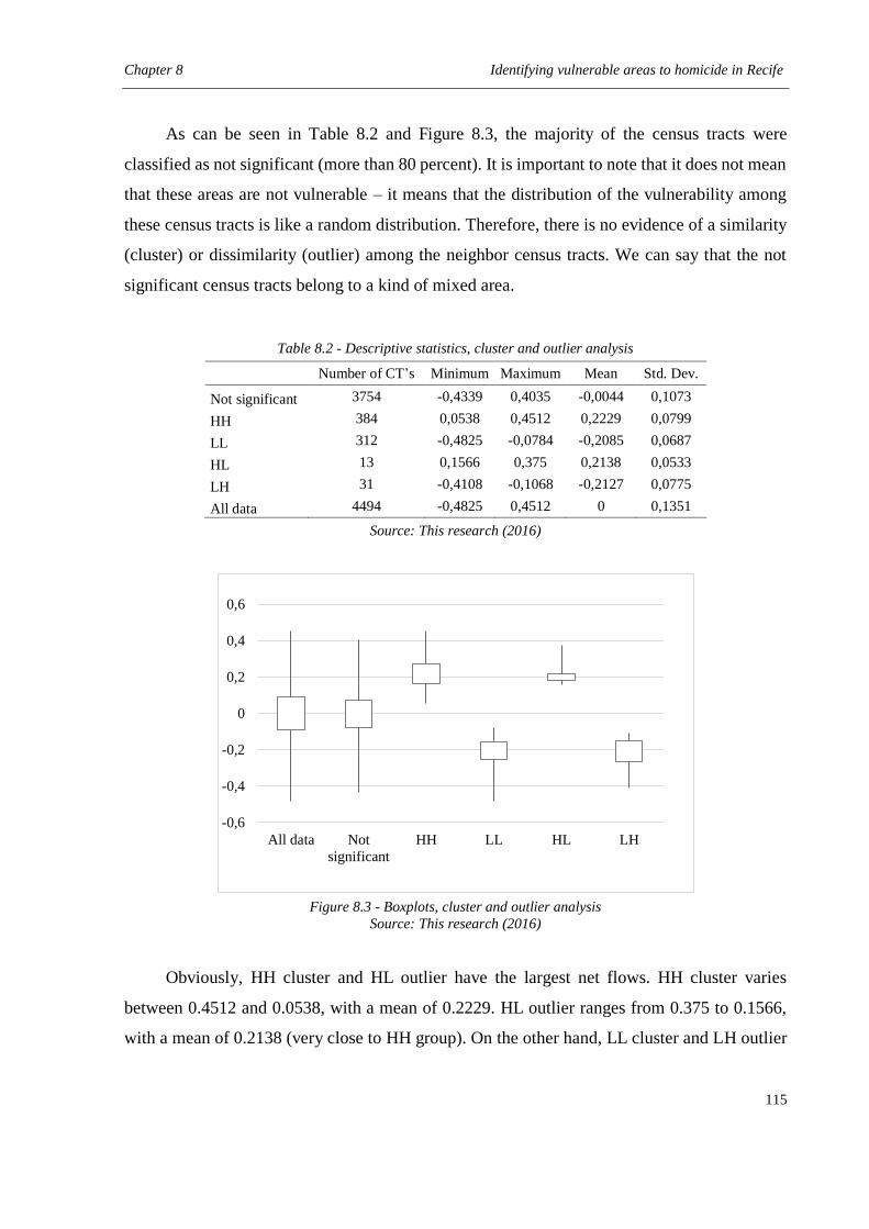
Chapter 8 Identifying vulnerable areas to homicide in Recife
115
As can be seen in Table 8.2 and Figure 8.3, the majority of the census tracts were
classified as not significant (more than 80 percent). It is important to note that it does not mean
that these areas are not vulnerable – it means that the distribution of the vulnerability among
these census tracts is like a random distribution. Therefore, there is no evidence of a similarity
(cluster) or dissimilarity (outlier) among the neighbor census tracts. We can say that the not
significant census tracts belong to a kind of mixed area.
Table 8.2 - Descriptive statistics, cluster and outlier analysis
Number of CT’s Minimum Maximum Mean Std. Dev.
Not significant 3754 -0,4339 0,4035 -0,0044 0,1073
HH 384 0,0538 0,4512 0,2229 0,0799
LL 312 -0,4825 -0,0784 -0,2085 0,0687
HL 13 0,1566 0,375 0,2138 0,0533
LH 31 -0,4108 -0,1068 -0,2127 0,0775
All data 4494 -0,4825 0,4512 0 0,1351
Source: This research (2016)
Figure 8.3 - Boxplots, cluster and outlier analysis
Source: This research (2016)
Obviously, HH cluster and HL outlier have the largest net flows. HH cluster varies
between 0.4512 and 0.0538, with a mean of 0.2229. HL outlier ranges from 0.375 to 0.1566,
with a mean of 0.2138 (very close to HH group). On the other hand, LL cluster and LH outlier
-0,6
-0,4
-0,2
0
0,2
0,4
0,6
All data Not
significant
HH LL HL LH
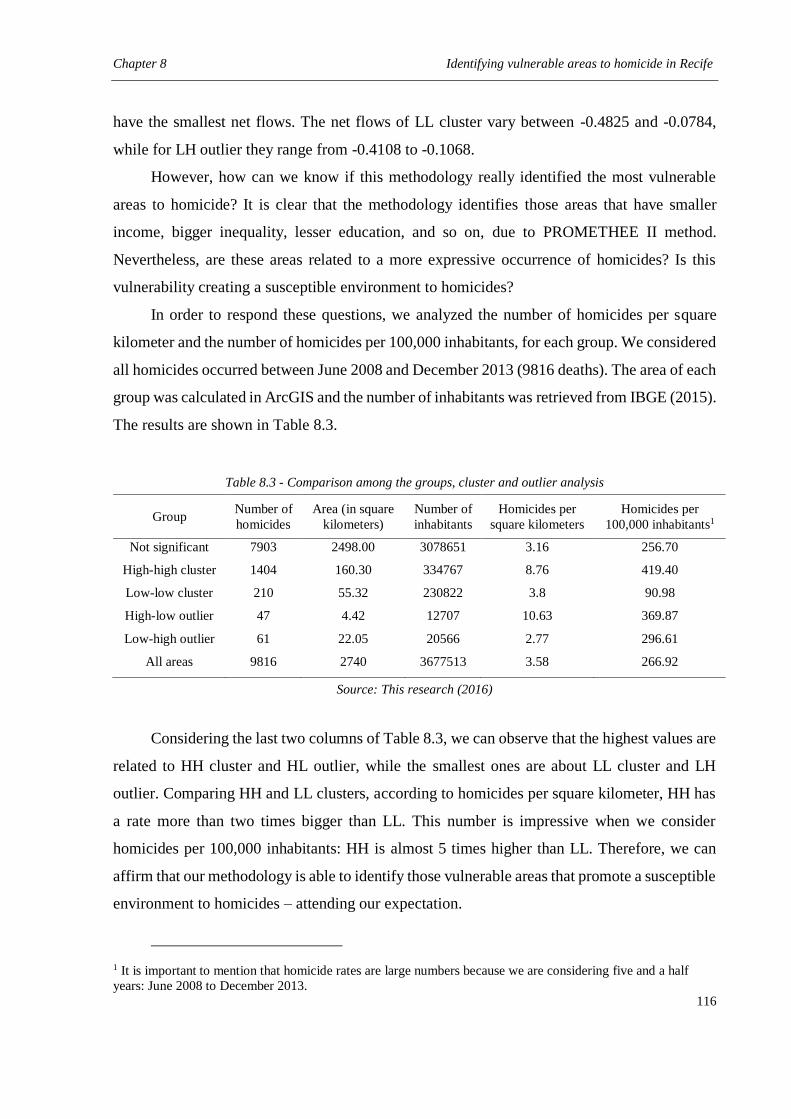
Chapter 8 Identifying vulnerable areas to homicide in Recife
116
have the smallest net flows. The net flows of LL cluster vary between -0.4825 and -0.0784,
while for LH outlier they range from -0.4108 to -0.1068.
However, how can we know if this methodology really identified the most vulnerable
areas to homicide? It is clear that the methodology identifies those areas that have smaller
income, bigger inequality, lesser education, and so on, due to PROMETHEE II method.
Nevertheless, are these areas related to a more expressive occurrence of homicides? Is this
vulnerability creating a susceptible environment to homicides?
In order to respond these questions, we analyzed the number of homicides per square
kilometer and the number of homicides per 100,000 inhabitants, for each group. We considered
all homicides occurred between June 2008 and December 2013 (9816 deaths). The area of each
group was calculated in ArcGIS and the number of inhabitants was retrieved from IBGE (2015).
The results are shown in Table 8.3.
Table 8.3 - Comparison among the groups, cluster and outlier analysis
Group Number of
homicides
Area (in square
kilometers)
Number of
inhabitants
Homicides per
square kilometers
Homicides per
100,000 inhabitants1
Not significant 7903 2498.00 3078651 3.16 256.70
High-high cluster 1404 160.30 334767 8.76 419.40
Low-low cluster 210 55.32 230822 3.8 90.98
High-low outlier 47 4.42 12707 10.63 369.87
Low-high outlier 61 22.05 20566 2.77 296.61
All areas 9816 2740 3677513 3.58 266.92
Source: This research (2016)
Considering the last two columns of Table 8.3, we can observe that the highest values are
related to HH cluster and HL outlier, while the smallest ones are about LL cluster and LH
outlier. Comparing HH and LL clusters, according to homicides per square kilometer, HH has
a rate more than two times bigger than LL. This number is impressive when we consider
homicides per 100,000 inhabitants: HH is almost 5 times higher than LL. Therefore, we can
affirm that our methodology is able to identify those vulnerable areas that promote a susceptible
environment to homicides – attending our expectation.
1 It is important to mention that homicide rates are large numbers because we are considering five and a half
years: June 2008 to December 2013.
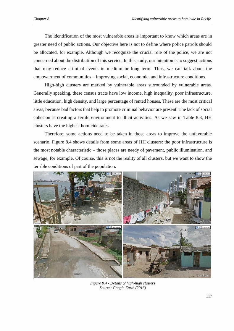
Chapter 8 Identifying vulnerable areas to homicide in Recife
117
The identification of the most vulnerable areas is important to know which areas are in
greater need of public actions. Our objective here is not to define where police patrols should
be allocated, for example. Although we recognize the crucial role of the police, we are not
concerned about the distribution of this service. In this study, our intention is to suggest actions
that may reduce criminal events in medium or long term. Thus, we can talk about the
empowerment of communities – improving social, economic, and infrastructure conditions.
High-high clusters are marked by vulnerable areas surrounded by vulnerable areas.
Generally speaking, these census tracts have low income, high inequality, poor infrastructure,
little education, high density, and large percentage of rented houses. These are the most critical
areas, because bad factors that help to promote criminal behavior are present. The lack of social
cohesion is creating a fertile environment to illicit activities. As we saw in Table 8.3, HH
clusters have the highest homicide rates.
Therefore, some actions need to be taken in those areas to improve the unfavorable
scenario. Figure 8.4 shows details from some areas of HH clusters: the poor infrastructure is
the most notable characteristic – those places are needy of pavement, public illumination, and
sewage, for example. Of course, this is not the reality of all clusters, but we want to show the
terrible conditions of part of the population.
Figure 8.4 - Details of high-high clusters
Source: Google Earth (2016)
Chapter 8 Identifying vulnerable areas to homicide in Recife
118
Infrastructure is an important factor to promote cohesion within a community. Faced with
a decent space, the population will take over the common space and create relationships,
bringing natural surveillance as consequence. The lack of infrastructure is not a normally
mentioned factor in the literature about social disorganization theory. Probably, this
characteristic is not remarkable in developed contexts, where this theory is largely discussed.
However, considering the Brazilian context, the lack of infrastructure is a relevant problem and
it seems to be closely associated to social cohesion.
Therefore, our first suggestion is the improvement of infrastructure in those areas. It is
hard to have quality of life when basic elements are not satisfied. However, this is not the only
problem of HH areas – this is the most notable. There is a deficiency in education too: the
literacy rate is the lowest in those census tracts. In this sense, more schools or schools with
more quality are needed. It is important to notice that something also must be made to control
school dropout – one needs to guarantee that the kids will show up in school, keeping them
away from illicit activities.
Other problems are related to low income and high inequality. Looking to Figure 8.4, it
is possible to see that these communities are very poor; and in one figure in particular, we can
observe the disparity between unfinished houses and luxurious buildings. An attempt to
minimize these problems may be the offer of better basic education and training courses to the
population. Because literacy is low in these areas, it must be hard to find a job with good wage.
Therefore, empowering these people may change their situation.
HL outliers are composed by census tracts with high vulnerability surrounded by low
vulnerability. The unfavorable situation of these areas are similar to HH clusters – the problems
and the suggestions to solve them can be the same. Nevertheless, the difference is that the
neighborhood is developed. Therefore, the displacement of offenders from the vulnerable area
to the favorable area may occur. The ideal situation would be to create an equality among the
areas, strengthening the vulnerable one.
It is important to mention that in Recife, like in many other places in Brazil, it is common
to create housing projects in risky communities. These communities are transferred to other
places, theoretically with better housing conditions. However, sometimes these action are not
successful. Normally, the communities are transferred to far areas and the residents do not
consider the new place as home. Therefore, we want to comment that maybe this is not the best
option to solve the problem – to move the vulnerable area to other space. With the creation of
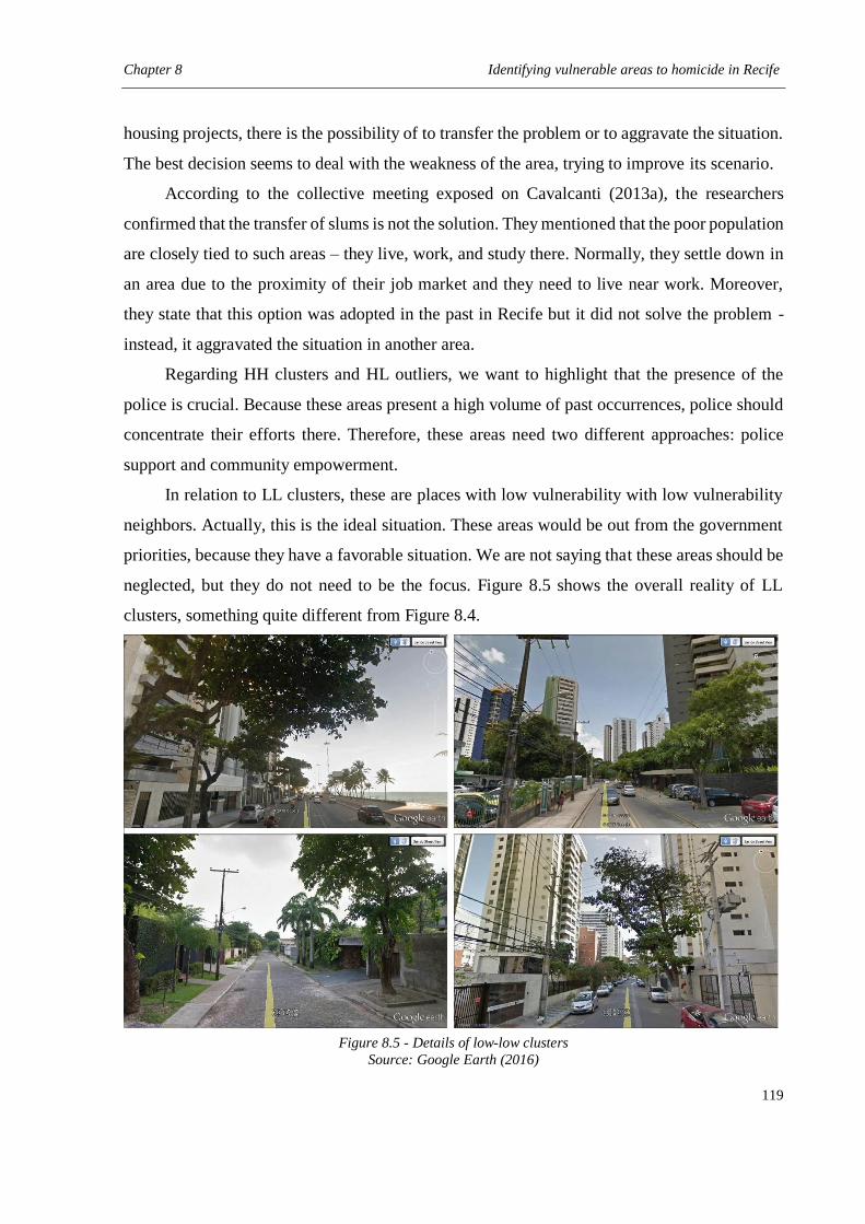
Chapter 8 Identifying vulnerable areas to homicide in Recife
119
housing projects, there is the possibility of to transfer the problem or to aggravate the situation.
The best decision seems to deal with the weakness of the area, trying to improve its scenario.
According to the collective meeting exposed on Cavalcanti (2013a), the researchers
confirmed that the transfer of slums is not the solution. They mentioned that the poor population
are closely tied to such areas – they live, work, and study there. Normally, they settle down in
an area due to the proximity of their job market and they need to live near work. Moreover,
they state that this option was adopted in the past in Recife but it did not solve the problem -
instead, it aggravated the situation in another area.
Regarding HH clusters and HL outliers, we want to highlight that the presence of the
police is crucial. Because these areas present a high volume of past occurrences, police should
concentrate their efforts there. Therefore, these areas need two different approaches: police
support and community empowerment.
In relation to LL clusters, these are places with low vulnerability with low vulnerability
neighbors. Actually, this is the ideal situation. These areas would be out from the government
priorities, because they have a favorable situation. We are not saying that these areas should be
neglected, but they do not need to be the focus. Figure 8.5 shows the overall reality of LL
clusters, something quite different from Figure 8.4.
Figure 8.5 - Details of low-low clusters
Source: Google Earth (2016)
Chapter 8 Identifying vulnerable areas to homicide in Recife
120
As can be seen in Figure 8.5, LL clusters are marked by wealthy neighborhoods.
Generally speaking, these areas are composed by buildings and large houses, with good
infrastructure and a woody environment. In these places, we can note that it is easier to take
over the common space and create relations. Although, the walls from buildings and houses
may reduce the natural surveillance.
Finally, we can talk about LH outliers – areas with low vulnerability surrounded by high
vulnerability. These areas present a favorable situation, but the neighbors are problematic.
Therefore, we suggest police effort in these places, because possible offenders (from the
neighbors) can commit delicts in the favorable areas. It is important to avoid crime displacement
to LH places. These are very interesting clusters because they are able to keep out the crime
despite being surrounding by high crime areas. In a sense, they are special and important to
understand.
From this analysis, we were able to identify the most critical areas regarding homicides
in Recife. This analysis allowed us to measure the vulnerability of each census tracts and
compared them to their neighbors. Through the clusters and outliers created by local Moran’s
I, we suggested preliminary actions to each group.
However, we concluded that the analysis considering all Metropolitan Region of Recife
is too comprehensive. The ideal is to apply the methodology in smaller areas, that will bring a
different result. Because PROMETHE II makes pairwise comparisons to measure the net
outranking flow to each alternative, the vulnerability of one census tract depends on all census
tracts. When we compare a large area, a large heterogeneity may be exist, modifying the results.
Due to this situation, we applied our methodology on Boa Viagem neighborhood and the results
are shown in Chapter 9.
8.5 Final comments
This chapter had the intention of to perform a preliminary attempt to identify the most
vulnerable areas to homicide in Recife. We applied PROMETHEE II method considering
income, inequality, education, population density, public illumination, and rented houses. Next,
we measured local Moran’s I to take into account the surrounding of each census tract.
Therefore, we were able to identify the clusters and outliers from Metropolitan Region of
Recife.
Chapter 8 Identifying vulnerable areas to homicide in Recife
121
High-high clusters are the most critical areas of the city, because they are vulnerable areas
with vulnerable neighbors. These census tracts should be the priority of public actions, because
they are responsible for the largest homicide rates. On the other hand, low-low clusters are
favorable areas surrounded by favorable areas. Therefore, these CTs do not need to be
government’s priority. They need to be understood though, so their LL cluster status can be
maintained. High-low and low-high outliers need some attention because of crime displacement
– low vulnerability areas can be affect by high vulnerable neighbors.
The identification of these areas is important because it is an attempt to better allocate
public resources concerned in reducing criminality. We believe that improving social cohesion
within vulnerable areas, we can expect a decrease in crime rates. Such a strategy will only bring
consequences in medium and long term, but it will cause deep transformations on the
unfavorable communities. Although our focus is suggesting strengthening actions for the
communities, we do not ignore the relevant role of the police – these approaches must work
together.
Chapter 9 Identifying vulnerable areas to homicide in Boa Viagem neighborhood
122
9 IDENTIFYING VULNERABLE AREAS TO HOMICIDE IN BOA VIAGEM NEIGHBORHOOD
In Chapter 8, we concluded that the identification of vulnerable areas might be more
accurate when we consider smaller areas. Due to this assumption, we also analyzed the most
vulnerable areas to homicide in a neighborhood instead of in a metropolitan region. We chose
Boa Viagem neighborhood to perform the study.
We employed three approaches to assess the most critical areas. The results from these
three attempts are similar and can be used together, but we selected only one to make a deep
analysis. We believe that the best option is to group some census tracts by similarity and then
to apply PROMETHEE II method. This methodology was able to order the groups, considering
vulnerability to homicides. After this ordering, one can suggest actions to improve social
cohesion and, consequently, it may reduce criminality.
9.1 Purpose of this chapter
The objective of this chapter is to answer: which are the most vulnerable areas to homicide
in Boa Viagem neighborhood? The aim here is almost the same from Chapter 8, but the local
of analysis is different. We are applying the methodology in a smaller area, since we trust that
the result will be more accurate. PROMETHEE II method does pairwise comparison among all
census tracts, so the heterogeneity of large areas can affect the results. Moreover, it is easier to
compare different approaches and discuss which one is the most suitable when we are working
with a reduced area. When we are working with big areas, it is hard to identify advantages and
disadvantages of the methodology.
To answer the research question, we employed three different approaches. In the first
attempt, we used PROMETHEE II method and ordered the census tracts according to their net
outranking flows. Secondly, we grouped some census tracts and applied PROMETHEE II for
these groups, ordering them. Finally, we used the same methodology from Chapter 8 –
PROMETHEE II and local Moran’s I. We consider that the second approach is the best option
here; however, all of them generates good results.
Our expectation is identical from Chapter 8 – to suggest a useful methodology to identify
the most vulnerable areas to homicide. The contributions also are the same but, in this
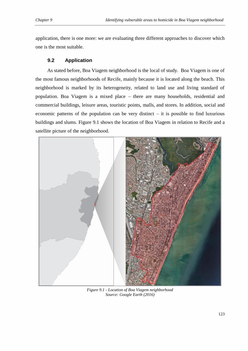
Chapter 9 Identifying vulnerable areas to homicide in Boa Viagem neighborhood
123
application, there is one more: we are evaluating three different approaches to discover which
one is the most suitable.
9.2 Application
As stated before, Boa Viagem neighborhood is the local of study. Boa Viagem is one of
the most famous neighborhoods of Recife, mainly because it is located along the beach. This
neighborhood is marked by its heterogeneity, related to land use and living standard of
population. Boa Viagem is a mixed place – there are many households, residential and
commercial buildings, leisure areas, touristic points, malls, and stores. In addition, social and
economic patterns of the population can be very distinct – it is possible to find luxurious
buildings and slums. Figure 9.1 shows the location of Boa Viagem in relation to Recife and a
satellite picture of the neighborhood.
Figure 9.1 - Location of Boa Viagem neighborhood
Source: Google Earth (2016)
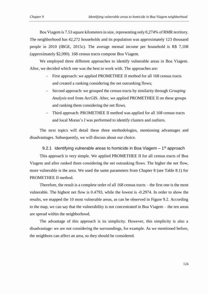
Chapter 9 Identifying vulnerable areas to homicide in Boa Viagem neighborhood
124
Boa Viagem is 7.53 square kilometers in size, representing only 0,274% of RMR territory.
The neighborhood has 42,272 households and its population was approximately 123 thousand
people in 2010 (IBGE, 2015c). The average mensal income per household is R$ 7,108
(approximately $2,090). 168 census tracts compose Boa Viagem.
We employed three different approaches to identify vulnerable areas in Boa Viagem.
After, we decided which one was the best to work with. The approaches are:
First approach: we applied PROMETHEE II method for all 168 census tracts
and created a ranking considering the net outranking flows;
Second approach: we grouped the census tracts by similarity through Grouping
Analysis tool from ArcGIS. After, we applied PROMETHEE II on these groups
and ranking them considering the net flows.
Third approach: PROMETHEE II method was applied for all 168 census tracts
and local Moran’s I was performed to identify clusters and outliers.
The next topics will detail these three methodologies, mentioning advantages and
disadvantages. Subsequently, we will discuss about our choice.
9.2.1 Identifying vulnerable areas to homicide in Boa Viagem – 1st approach
This approach is very simple. We applied PROMETHEE II for all census tracts of Boa
Viagem and after ranked them considering the net outranking flows. The higher the net flow,
more vulnerable is the area. We used the same parameters from Chapter 8 (see Table 8.1) for
PROMETHEE II method.
Therefore, the result is a complete order of all 168 census tracts – the first one is the most
vulnerable. The highest net flow is 0.4793, while the lowest is -0.2974. In order to show the
results, we mapped the 10 most vulnerable areas, as can be observed in Figure 9.2. According
to the map, we can say that the vulnerability is not concentrated in Boa Viagem – the ten areas
are spread within the neighborhood.
The advantage of this approach is its simplicity. However, this simplicity is also a
disadvantage: we are not considering the surroundings, for example. As we mentioned before,
the neighbors can affect an area, so they should be considered.
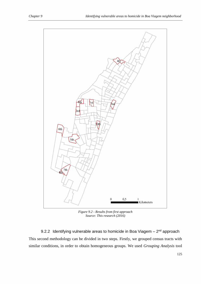
Chapter 9 Identifying vulnerable areas to homicide in Boa Viagem neighborhood
125
Figure 9.2 - Results from first approach
Source: This research (2016)
9.2.2 Identifying vulnerable areas to homicide in Boa Viagem – 2nd approach
This second methodology can be divided in two steps. Firstly, we grouped census tracts with
similar conditions, in order to obtain homogeneous groups. We used Grouping Analysis tool
Chapter 9 Identifying vulnerable areas to homicide in Boa Viagem neighborhood
126
from ArcGIS to create the groups. Figure 9.3 shows the map of Boa Viagem divided by 13
groups.
Figure 9.3 - Division of Boa Viagem into 13 groups
Source: This research (2016)
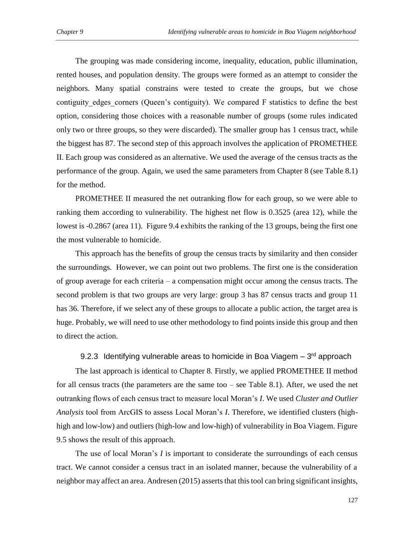
Chapter 9 Identifying vulnerable areas to homicide in Boa Viagem neighborhood
127
The grouping was made considering income, inequality, education, public illumination,
rented houses, and population density. The groups were formed as an attempt to consider the
neighbors. Many spatial constrains were tested to create the groups, but we chose
contiguity_edges_corners (Queen’s contiguity). We compared F statistics to define the best
option, considering those choices with a reasonable number of groups (some rules indicated
only two or three groups, so they were discarded). The smaller group has 1 census tract, while
the biggest has 87. The second step of this approach involves the application of PROMETHEE
II. Each group was considered as an alternative. We used the average of the census tracts as the
performance of the group. Again, we used the same parameters from Chapter 8 (see Table 8.1)
for the method.
PROMETHEE II measured the net outranking flow for each group, so we were able to
ranking them according to vulnerability. The highest net flow is 0.3525 (area 12), while the
lowest is -0.2867 (area 11). Figure 9.4 exhibits the ranking of the 13 groups, being the first one
the most vulnerable to homicide.
This approach has the benefits of group the census tracts by similarity and then consider
the surroundings. However, we can point out two problems. The first one is the consideration
of group average for each criteria – a compensation might occur among the census tracts. The
second problem is that two groups are very large: group 3 has 87 census tracts and group 11
has 36. Therefore, if we select any of these groups to allocate a public action, the target area is
huge. Probably, we will need to use other methodology to find points inside this group and then
to direct the action.
9.2.3 Identifying vulnerable areas to homicide in Boa Viagem – 3rd approach
The last approach is identical to Chapter 8. Firstly, we applied PROMETHEE II method
for all census tracts (the parameters are the same too – see Table 8.1). After, we used the net
outranking flows of each census tract to measure local Moran’s I. We used Cluster and Outlier
Analysis tool from ArcGIS to assess Local Moran’s I. Therefore, we identified clusters (high-
high and low-low) and outliers (high-low and low-high) of vulnerability in Boa Viagem. Figure
9.5 shows the result of this approach.
The use of local Moran’s I is important to considerate the surroundings of each census
tract. We cannot consider a census tract in an isolated manner, because the vulnerability of a
neighbor may affect an area. Andresen (2015) asserts that this tool can bring significant insights,
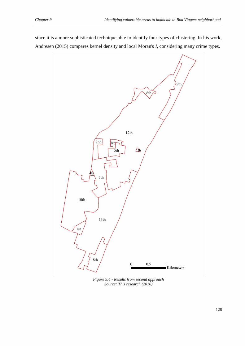
Chapter 9 Identifying vulnerable areas to homicide in Boa Viagem neighborhood
128
since it is a more sophisticated technique able to identify four types of clustering. In his work,
Andresen (2015) compares kernel density and local Moran's I, considering many crime types.
Figure 9.4 - Results from second approach
Source: This research (2016)
Chapter 9 Identifying vulnerable areas to homicide in Boa Viagem neighborhood
129
This methodology has the advantage of to take into account the surroundings. However,
we believe that many areas were considered as “not significant” – more than 88 percent.
Overall, only three areas are categorized as high-high cluster – it is possible that some
vulnerable areas were left out of this classification.
Figure 9.5 - Results from third approach
Source: This research (2016)
Chapter 9 Identifying vulnerable areas to homicide in Boa Viagem neighborhood
130
Looking to the results of these three approaches, we can see that the results are similar.
The census tracts classified as most vulnerable may not be the same, but the regions are
common. Therefore, we can say that our three techniques show some similarities and
consistencies. All three approaches are useful and they can be used combined or separately. In
order to justify the use of public resources, one may want to rely on more than one piece of
information, so the techniques can be considered together. The argument to implement crime
prevention can be stronger when more than one technique confirms the necessity of an area.
We are aware of the power of these three approaches combined, but we opted to consider
only one to continue our analysis. Will be easier to explore the results taking into account only
one of our techniques. We chose the second approach, which involves grouping analysis and
PROMETHEE II. The first methodology was disregarded because it does not consider the
surroundings and the third one was ignored because of the classification of many areas as “not
significant”. Second approach takes into account the surroundings and gives a complete order
of the areas.
Regarding the second approach, the question about some large areas is not a big problem,
since these areas can be seen as low vulnerability. If these areas were in the top of the ranking,
it would be a concern. The information would not be useful for public agencies, because they
could not implement a crime reduction strategy that targeted a large area. Since our approach
identified the small groups as highest risks, the result is useful to identify areas for intervention.
The two largest areas are ranked on the two lowest positions (low vulnerability).
9.3 Results and discussion
In this subsection, we are going to present the results of the second approach in details
and make the pertinent discussions. Table 9.1 shows the net outranking flow of each group and
the ranking. It is important to remember that the higher the net flow, the higher the vulnerability.
Therefore, area 12 is the most vulnerable, while area 11 is the less vulnerable.
According to Table 9.1, Groups 12, 4, 5, 9, and 6 are the most vulnerable to homicides.
These areas are composed by 2, 3, 2, 1, and 2 census tracts, respectively. We will show some
details about these five most vulnerable groups, in order to understand why they were classified
like this. With this analysis, we can detect the weakness of each area, which will help to define
specific strategies later.
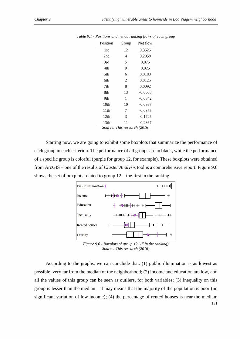
Chapter 9 Identifying vulnerable areas to homicide in Boa Viagem neighborhood
131
Table 9.1 - Positions and net outranking flows of each group
Position Group Net flow
1st 12 0,3525
2nd 4 0,2058
3rd 5 0,075
4th 9 0,025
5th 6 0,0183
6th 2 0,0125
7th 8 0,0092
8th 13 -0,0008
9th 1 -0,0642
10th 10 -0,0867
11th 7 -0,0875
12th 3 -0,1725
13th 11 -0,2867
Source: This research (2016)
Starting now, we are going to exhibit some boxplots that summarize the performance of
each group in each criterion. The performance of all groups are in black, while the performance
of a specific group is colorful (purple for group 12, for example). These boxplots were obtained
from ArcGIS – one of the results of Cluster Analysis tool is a comprehensive report. Figure 9.6
shows the set of boxplots related to group 12 – the first in the ranking.
Figure 9.6 - Boxplots of group 12 (1st in the ranking)
Source: This research (2016)
According to the graphs, we can conclude that: (1) public illumination is as lowest as
possible, very far from the median of the neighborhood; (2) income and education are low, and
all the values of this group can be seen as outliers, for both variables; (3) inequality on this
group is lesser than the median – it may means that the majority of the population is poor (no
significant variation of low income); (4) the percentage of rented houses is near the median;
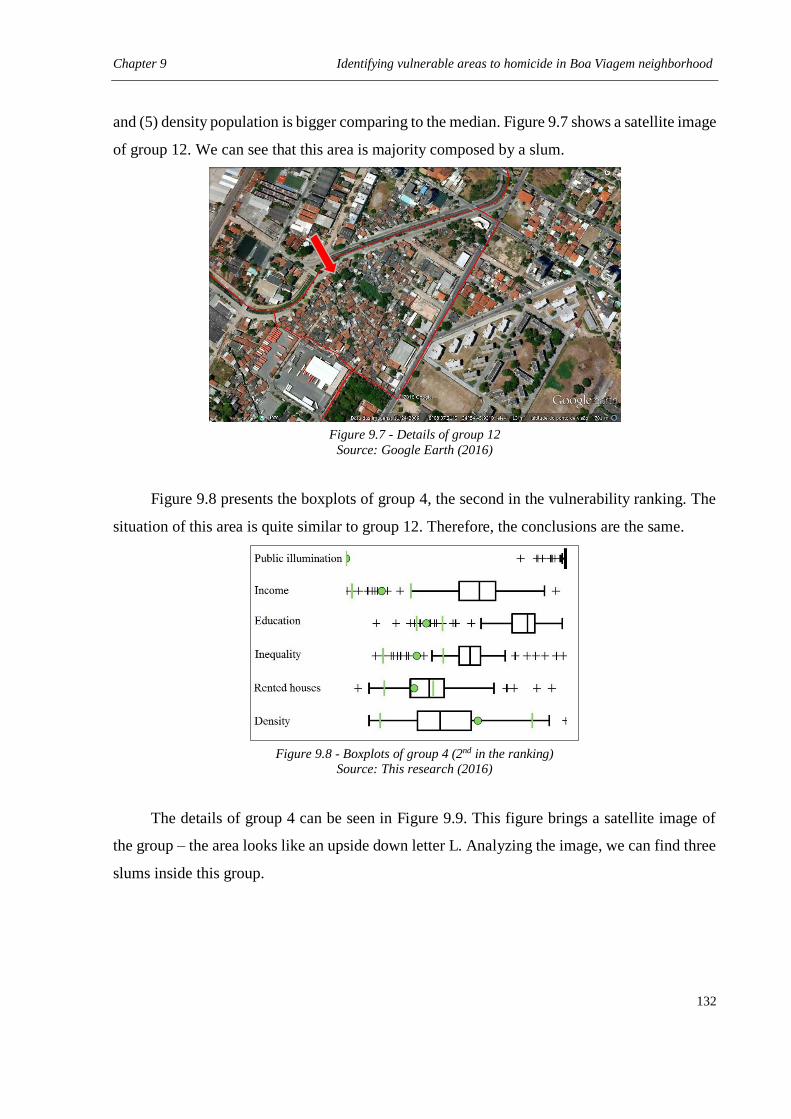
Chapter 9 Identifying vulnerable areas to homicide in Boa Viagem neighborhood
132
and (5) density population is bigger comparing to the median. Figure 9.7 shows a satellite image
of group 12. We can see that this area is majority composed by a slum.
Figure 9.7 - Details of group 12
Source: Google Earth (2016)
Figure 9.8 presents the boxplots of group 4, the second in the vulnerability ranking. The
situation of this area is quite similar to group 12. Therefore, the conclusions are the same.
Figure 9.8 - Boxplots of group 4 (2nd in the ranking)
Source: This research (2016)
The details of group 4 can be seen in Figure 9.9. This figure brings a satellite image of
the group – the area looks like an upside down letter L. Analyzing the image, we can find three
slums inside this group.
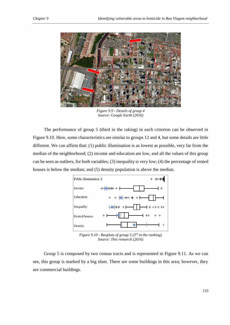
Chapter 9 Identifying vulnerable areas to homicide in Boa Viagem neighborhood
133
Figure 9.9 - Details of group 4
Source: Google Earth (2016)
The performance of group 5 (third in the raking) in each criterion can be observed in
Figure 9.10. Here, some characteristics are similar to groups 12 and 4, but some details are little
different. We can affirm that: (1) public illumination is as lowest as possible, very far from the
median of the neighborhood; (2) income and education are low, and all the values of this group
can be seen as outliers, for both variables; (3) inequality is very low; (4) the percentage of rented
houses is below the median; and (5) density population is above the median.
Figure 9.10 - Boxplots of group 5 (3rd in the ranking)
Source: This research (2016)
Group 5 is composed by two census tracts and is represented in Figure 9.11. As we can
see, this group is marked by a big slum. There are some buildings in this area; however, they
are commercial buildings.
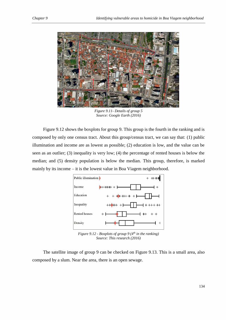
Chapter 9 Identifying vulnerable areas to homicide in Boa Viagem neighborhood
134
Figure 9.11- Details of group 5
Source: Google Earth (2016)
Figure 9.12 shows the boxplots for group 9. This group is the fourth in the ranking and is
composed by only one census tract. About this group/census tract, we can say that: (1) public
illumination and income are as lowest as possible; (2) education is low, and the value can be
seen as an outlier; (3) inequality is very low; (4) the percentage of rented houses is below the
median; and (5) density population is below the median. This group, therefore, is marked
mainly by its income – it is the lowest value in Boa Viagem neighborhood.
Figure 9.12 - Boxplots of group 9 (4th in the ranking)
Source: This research (2016)
The satellite image of group 9 can be checked on Figure 9.13. This is a small area, also
composed by a slum. Near the area, there is an open sewage.
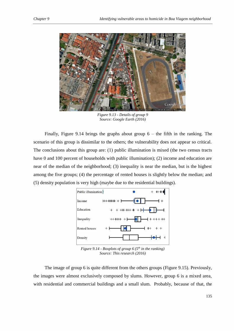
Chapter 9 Identifying vulnerable areas to homicide in Boa Viagem neighborhood
135
Figure 9.13 - Details of group 9
Source: Google Earth (2016)
Finally, Figure 9.14 brings the graphs about group 6 – the fifth in the ranking. The
scenario of this group is dissimilar to the others; the vulnerability does not appear so critical.
The conclusions about this group are: (1) public illumination is mixed (the two census tracts
have 0 and 100 percent of households with public illumination); (2) income and education are
near of the median of the neighborhood; (3) inequality is near the median, but is the highest
among the five groups; (4) the percentage of rented houses is slightly below the median; and
(5) density population is very high (maybe due to the residential buildings).
Figure 9.14 - Boxplots of group 6 (5th in the ranking)
Source: This research (2016)
The image of group 6 is quite different from the others groups (Figure 9.15). Previously,
the images were almost exclusively composed by slums. However, group 6 is a mixed area,
with residential and commercial buildings and a small slum. Probably, because of that, the
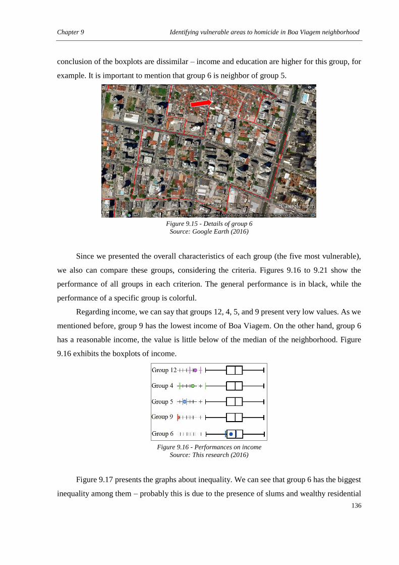
Chapter 9 Identifying vulnerable areas to homicide in Boa Viagem neighborhood
136
conclusion of the boxplots are dissimilar – income and education are higher for this group, for
example. It is important to mention that group 6 is neighbor of group 5.
Figure 9.15 - Details of group 6
Source: Google Earth (2016)
Since we presented the overall characteristics of each group (the five most vulnerable),
we also can compare these groups, considering the criteria. Figures 9.16 to 9.21 show the
performance of all groups in each criterion. The general performance is in black, while the
performance of a specific group is colorful.
Regarding income, we can say that groups 12, 4, 5, and 9 present very low values. As we
mentioned before, group 9 has the lowest income of Boa Viagem. On the other hand, group 6
has a reasonable income, the value is little below of the median of the neighborhood. Figure
9.16 exhibits the boxplots of income.
Figure 9.16 - Performances on income
Source: This research (2016)
Figure 9.17 presents the graphs about inequality. We can see that group 6 has the biggest
inequality among them – probably this is due to the presence of slums and wealthy residential
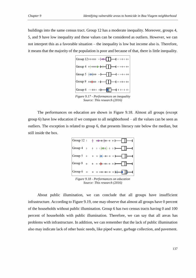
Chapter 9 Identifying vulnerable areas to homicide in Boa Viagem neighborhood
137
buildings into the same census tract. Group 12 has a moderate inequality. Moreover, groups 4,
5, and 9 have low inequality and these values can be considered as outliers. However, we can
not interpret this as a favorable situation – the inequality is low but income also is. Therefore,
it means that the majority of the population is poor and because of that, there is little inequality.
Figure 9.17 - Performances on inequality
Source: This research (2016)
The performances on education are shown in Figure 9.18. Almost all groups (except
group 6) have low education if we compare to all neighborhood – all the values can be seen as
outliers. The exception is related to group 6, that presents literacy rate below the median, but
still inside the box.
Figure 9.18 - Performances on education
Source: This research (2016)
About public illumination, we can conclude that all groups have insufficient
infrastructure. According to Figure 9.19, one may observe that almost all groups have 0 percent
of the households without public illumination. Group 6 has two census tracts having 0 and 100
percent of households with public illumination. Therefore, we can say that all areas has
problems with infrastructure. In addition, we can remember that the lack of public illumination
also may indicate lack of other basic needs, like piped water, garbage collection, and pavement.
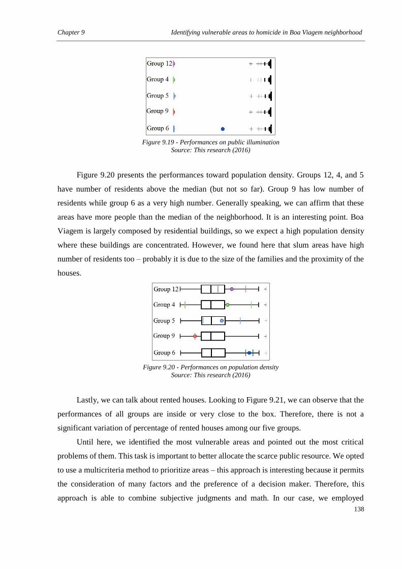
Chapter 9 Identifying vulnerable areas to homicide in Boa Viagem neighborhood
138
Figure 9.19 - Performances on public illumination
Source: This research (2016)
Figure 9.20 presents the performances toward population density. Groups 12, 4, and 5
have number of residents above the median (but not so far). Group 9 has low number of
residents while group 6 as a very high number. Generally speaking, we can affirm that these
areas have more people than the median of the neighborhood. It is an interesting point. Boa
Viagem is largely composed by residential buildings, so we expect a high population density
where these buildings are concentrated. However, we found here that slum areas have high
number of residents too – probably it is due to the size of the families and the proximity of the
houses.
Figure 9.20 - Performances on population density
Source: This research (2016)
Lastly, we can talk about rented houses. Looking to Figure 9.21, we can observe that the
performances of all groups are inside or very close to the box. Therefore, there is not a
significant variation of percentage of rented houses among our five groups.
Until here, we identified the most vulnerable areas and pointed out the most critical
problems of them. This task is important to better allocate the scarce public resource. We opted
to use a multicriteria method to prioritize areas – this approach is interesting because it permits
the consideration of many factors and the preference of a decision maker. Therefore, this
approach is able to combine subjective judgments and math. In our case, we employed
Chapter 9 Identifying vulnerable areas to homicide in Boa Viagem neighborhood
139
PROMETHEE II method to rank some areas of Boa Viagem neighborhood, considering
vulnerability to homicides. This neighborhood is very heterogeneous, marked by extremes –
wealthy buildings and slums. Of course that our methodology selected the slums as the most
vulnerable areas, since these places have lower income, education, and infrastructure for
example.
Figure 9.21 - Performances on rented houses
Source: This research (2016)
After the prioritization, it is important to define which actions will be allocated in each
local, in order to decrease homicide rates. We recognize the important role of the police in
combating violence, but we think that this effort needs to be combined with more
comprehensive strategies. In this sense, we are going to discuss about changing the social and
economic situations of vulnerable areas. Public security is not strictly related to police
intervention – violence must be treated with integrated politics, offering equal opportunities for
the population. Therefore, in this study, we aim to debate about public actions that can be taken
to fortify communities.
Actually, none of the approaches can be neglected (police effort and strengthening
actions). Pernambuco State Government (2007) believes that prevention and repression
strategies must be complementary and simultaneous. Therefore, actions to improve police work
and criminal system are required. In relation to the police, the increasing of police effort,
capacitation of cops, and fleet renewal, are examples of actions. About the criminal system, one
can suggest better prison conditions, improved information system, and resocialization. These
actions do not deal with the cause of the violence, but they are essential since they avoid the
loss of new lives and guarantee human rights.
On the other hand, prevention strategies are crucial as well. Pernambuco State
Government (2007) affirms that prevention actions are multidisciplinary, increasing protection
factors and reducing risk factors. Pact of Life involves many programs related to social
Chapter 9 Identifying vulnerable areas to homicide in Boa Viagem neighborhood
140
prevention: community intervention; violence prevention in schools; inclusion in job market;
mediation of conflicts; arts, culture, and sports; and treatment for drug users, for example. In
addition, PFL is also aimed to support victims and offenders: protection to victims,
resocialization, support to young offenders, education and professionalization of offenders, and
assistance to offender’s families.
Moreover, there are also situational prevention actions. These movements have the
objective of to reduce environmental conditions that may increase the occurrence of crimes.
The projects associated to this theme can be improvement of public illumination, integration of
isolated urban spaces, security on public transport and bus stops, creation and maintenance of
leisure areas, and expansion of natural surveillance.
Therefore, we can highlight the importance of integrated actions. In 2007, Pernambuco
State Government recognized that the reduction of violence just would be achieved with an
integrated strategy, involving prevention and combating actions. Pact of Life program proves
that. The International Centre for the Prevention of Crime (ICPC) (ICPC, 2010) also agree that
the combination of many approaches is useful for crime prevention.
According to Velasquez (2013), security politics must be comprehensive, from the
prevention of risk factors to coercive measures. Within the prevention actions, he cites antidrug
programs, attention to vulnerable groups, and strengthen of citizenship. The other group of
actions may involve improvement of penitentiary system, better collection of data, and
resocialization. Cavalcanti (2013b) complements saying that beyond the social investment, one
must invest in police too: more men, better wages, more preparation, motivation, and respect.
In Cavalcanti (2013c), some requirements are pointed out for integrated human security
politics. Some of these requirements are integrated actions, strong leadership, trustful and
transparent data, mixed programs and strategies, the understanding that violence is not a
problem specific from the police, to face violence as an economic problem too, to control risk
factors (drugs, prostitution, guns, alcohol), and to consider action from the prevention to the
punishment.
UNODC (2008) defends that “repression and enforcement are not the most effective ways
to prevent crime and reduce victimization”. They believe that crime reduction may come
through law reform and commitment to human rights. The report of UNODC (2008) shows
some crime prevention programs in the Caribbean and Southern Africa (developing areas) and
according them, the following strategies are successful in reducing violence: enhancing parent
Chapter 9 Identifying vulnerable areas to homicide in Boa Viagem neighborhood
141
skills, preschool literacy, improvement of school curriculum, restorative justice for youths, drug
and alcohol treatment, and treatment-based corrections.
Therefore, according to the mentioned works, there is a consensus that integrated
strategies are the best option to deal with violence. Many actions should be taken
simultaneously to reduce crime rates, involving different aspects. The presence of the police is
important to avoid the increase of number of victims and the criminal system needs to be
trustful. Moreover, the life condition of the population should be improved, bringing
opportunities, social cohesion, and reduction of the attractiveness of illicit activities. In this
study, our objective is to explore the second set of strategies.
The reduction of violence (and mainly homicide rates) through social, economic, and
urban strategies is being applied (with success) in some places. These successful cases should
be analyzed – we can learn with these places and apply similar strategy here. Of course, we
need to consider some differences between Brazil and other countries, but this kind of study of
can be very instructive. ICPC (2010) defends that the strategies must respect the conditions and
priorities of the place. Replication of actions must to be done with caution, giving space to
adaption.
Therefore, crime rates may be reduced improving the quality of life of the population.
According to ICPC (2010), social and educational approaches to crime prevention “are
concerned with strengthening the capacities of individuals, families, or groups to live healthy,
productive and pro-social lives, and reduce their chances of being victimized or becoming
involved in offending. They include a wide range of practices, and are often targeted towards
families, children and young people, since these are the age groups most at risk.”.
The report of UNODC (2008) confirms our findings about the relation among homicide
with inequality and development. They found that, in developing countries, homicide is largely
positively associated with inequality and largely negatively associated with quality of life
(Human Development Index). In this way, a first step can be dealing with these problems.
In order to handle with inequality and low income, the better option seems to offer better
opportunities to the population – and it is closely related to education. Public power can offer,
for example, better schools, training courses, and preparation to job market to unfavorable
communities. UNODC (2008) affirms that, in developing countries, about 60 percent of the
prisoners are functionally illiterate. Therefore, we can see that there is a connection between
criminality and education (our environmental analysis confirms this too). Moreover, there is a
Chapter 9 Identifying vulnerable areas to homicide in Boa Viagem neighborhood
142
connection between education and wage. Normally, the better the education, the better is the
wage. In this way, the empowerment of the population can start with education, since this aspect
can affect many other dimensions.
Education must not be seen as an activity restricted to youths. However, early intervention
brings better results. Pernambuco State Government (2007) states that the highest incidence of
homicides in Pernambuco is among men and youths. The arrested people are mainly young
low-schooling men (and 24 percent of the prisoners were caught because of murders). These
number make we think that that youths are leaving school and involving in illicit activities.
Therefore, something need to be done to keep the youths busy and away from wrong
activities. ICPC (2010) shows that sports and cultural activities may be a successful strategy
for youths. These events “are seen to encourage self-expression and esteem, life skills and social
skills, and education, as well as providing diversionary activities to reduce opportunities for
offending, or exposure to risks of offending.”. ICPC (2010) still mention that initiatives related
to crime prevention are being largely assigned to youths. The reasons are known: the massive
presence of youths among offenders and the success of early intervention. The World Health
Organization, UNICEF, the Council of Europe and the Organization for Economic Co-
operation and Development have defended youths as center of crime prevention approaches.
Nevertheless, ICPC (2010) affirms that actions to modify the risk of crime should be
taken for neighborhoods too – not only for individuals or for specific groups. Strategies like
conflict mediation, creation of safe environment in schools, and citizenship training may help
to reduce crime in disadvantaged places. We want to include to this list the transformation of
urban space.
In Cavalcanti (2013a), some researchers debate about actions that are related to public
security. They observe that urbanism, mobility, education, culture, and cleanliness contribute
for a safer environment. These elements improve the urban space and the population can occupy
the area (we can say, increasing the social cohesion). Moreover, such alternatives also offer
education and leisure, which may reduce idleness (an open door for drugs, gangs, and
marginality). These actions may create a new social scenario, transforming the human relations.
Therefore, the public space can be transformed through education, leisure, culture, sports,
public transport, and public health.
The book of Cavalcanti (2013a) also brings a discussion about the layout of the
neighborhoods. In Recife, many streets have houses or buildings with high walls. It reduces the
Chapter 9 Identifying vulnerable areas to homicide in Boa Viagem neighborhood
143
natural vigilance and the socialization of the area and, consequently, it may turns the place less
safe. Therefore, the government can implement some rules in order to avoid this phenomenon:
they can prohibit high walls, for example, and suggest iron grilles.
Therefore, we can observe that the transformation of the urban space is crucial to improve
the quality of life. Giving better infrastructure to the population (pavement, piped water, public
illumination, adequate sewage) can be a first step. After the basic needs are supplied, other
actions can be done, like inserting leisure areas or improving public transport, for example.
Infrastructure also is an important factor to promote cohesion within a community. Therefore,
prevention politics may include projects toward urbanization, including illumination,
pavement, squares, gardens, and parks.
We can compare these strategies with the Primary, Secondary, and Tertiary model of
Brantingham & Faust (1976). The actions related to the empowerment of the population can be
inserted on the secondary level, since they aim to prevent potential offenders from moving into
criminal activities. Some examples of these strategies are: strengthening of communities at risk;
safer environment in schools, job opportunities, better schools, training courses, sports and arts
for youths, and mediation of conflicts in communities.
Moreover, the strategies about the transformation of urban space can be classified in
primary level, since they are related to environmental design. These actions may comprise, for
example: improvement of infrastructure (public illumination, pavement, sewage), construction
of leisure areas, improvement of collective transport, and programs to increase the natural
surveillance.
Here, we discussed distinct actions that should be implanted to reduce vulnerability and,
consequently, violence. These actions involve different factors (education and urban space, for
example), targets (individuals or neighborhoods), and time horizons (short, medium or long
terms). Therefore, we believe that holistic strategies may be successful to deal with this
problem.
9.4 Final comments
In this chapter, we developed an analysis to identify the most vulnerable areas toward
homicides in Boa Viagem. We performed this study because we concluded in Chapter 8 that
the evaluation on smaller areas might be more accurate, because of the heterogeneity and
pairwise comparison. We used three different approaches to assess the vulnerable areas and
Chapter 9 Identifying vulnerable areas to homicide in Boa Viagem neighborhood
144
they showed similar results. Our three approaches can be used together, in order to better justify
the allocation of public resource. On the other hand, any approach can be considered separately,
if one prefers simplify the analysis.
Since we know where the action must to be allocated, the next task is to define what need
to be done. It is clear that integrated strategies are the best option to deal with vulnerability –
police effort, community empowerment, and transformation of urban space. Each initiative will
contribute in a particular manner and the synergy of them may make the difference.
Here, we discussed mainly about the fortification of the population, social cohesion, and
urban transformations – these initiatives can cause deep changes in communities, conducting
to a reduction on criminality. The actions may not present an immediate effect, but the
consequences may be efficient and profound. Since the population is experiencing better life
conditions, the illicit activities may look less attractive. Violent places around the word
transformed their scenarios with good management and commitment of the population;
therefore, we can believe that it is also possible in Recife.
Chapter 10 Final remarks
145
10 FINAL REMARKS
This last chapter is aimed to present the final comments about this research, highlighting
the most important finding. Moreover, this chapter will present the implications and the
limitations that were found during this study. Finally, some suggestions will be given for future
works.
10.1 Conclusions
The conclusions of this thesis will be done according to the different analyses – temporal,
spatial, environmental, and multicriteria.
10.1.1 Temporal analysis
The seasonality of crime has been widely debated in the literature, although few
investigations had been made in regions with a tropical climate, particularly published in
international journals. This analysis had the aim of analyzing temporal variations of homicide
(considering seasons, months, days of week, and periods of week) in a city where the average
annual temperature is approximately 26˚C and the variation between months is not greater than
4.2˚C. Moreover, we conducted a spatial analysis taking into account all temporal units to
evaluate the similarity (or not) of spatial patterns across these units.
This analysis was led by two questions. The first one inquired if there is temporal
variation of homicides in Recife. After the tests with ANOVA, we can conclude that there is
not significant temporal variation for seasons and months. However, there is significant
variation between days of week and periods of day. Homicides in Recife are more frequent on
Saturdays (18.86 percent) and Sundays (23.1 percent), as well as during nights (37.21 percent)
and dawns (25.41 percent).
The second question asked if the spatial patterns would be different when we consider the
temporal units. The results of spatial point pattern tests showed that the patterns are distinct for
seasons, some days of week, periods of day, weekdays versus weekends, and days versus nights.
Moreover, the results indicate that the aggregation of homicides in any temporal dimension is
inappropriate when place matters, because there is not enough similarity between the spatial
patterns. In this study, we also concluded that the temporal variation of homicides in Recife can
be understood by the perspective of routine activity theory.
Chapter 10 Final remarks
146
10.1.2 Spatial analysis
Spatial analysis are instructive for theoretical and crime prevention considerations.
However, in the literature, one crime type is missing from these analyses: homicide. Though
homicide may be included in “all crime types” analysis, most often there are not enough
homicides for a meaningful analysis of their spatial crime patterns and concentrations.
Nevertheless, in Brazil, there is a large number of homicides so this kind of study is possible.
In this sense, we performed two analysis considering spatiality. Firstly, we investigated
the homicide concentration in the city of Recife. The findings revealed that homicides are very
concentrated in this place – between 2009 and 2013, all the homicide occurred in less than 10
percent of street segments. Annually, the percentage of street segments with homicides was not
above than 2.32 percent. Even though homicides being a rare event, this concentration is very
significant. In addition, homicides are staying more concentrated in the city of Recife across
the years: the concentration almost doubled in five years.
Secondly, the stability of spatial patterns was analyzed. When we considered homicides
by year, the spatial point pattern test showed that the patterns were not stable over years.
However, in Chapter 5, we concluded that annual aggregations are not appropriate for
homicides when spatiality is relevant. In this sense, SSPT was performed again but regarding
temporal dimensions. These second results revealed that there was stability of spatial patterns
along the years since the temporal units were taken into account. However, these findings are
not valid for weekdays and night/dawn.
10.1.3 Environmental analysis
According to the literature review about the determinants of homicide in Brazil, it became
clear that homicides are related to social disorganization theory. In this sense, we have
investigated the relationship between homicide in the census tracts of Recife and a set of
variables relating to this theory. Though we did not find statistically significant relationships
with the full set of explanatory variables, the results of the final model were instructive.
The spatial error regression showed that eight variables are statistically significant with
homicides in Recife. The model presents a positive relationship with inequality, rented houses,
and number of residents while it reveals a negative relation with income, education, public
illumination, population density, and street network density. As can be seen, all the variables
Chapter 10 Final remarks
147
have the expected behavior according to social disorganization theory. Moreover, it is important
to note that the most expressive variables of this model are income and inequality.
A particular note is that variables relating to conditions specific to a Brazilian context are
important. Though not all of the explanatory variables that may represent vulnerability were
statistically significant (open sewers, garbage, improvised housing, and electricity), public
illumination proved to be important in the expected direction. This supports the need to not
simply incorporate explanatory variables that represent social disorganization theory (or any
theory for that matter) in a developed context. There is definitely some generalizability of these
theories, but local conditions matter.
10.1.4 Multicriteria analysis
Since public resources are limited, some kind of prioritization is need to allocate them. In
this thesis, we propose a preliminary methodology to identify the most vulnerable areas in
Recife and Boa Viagem neighborhood. Through this methodology, the neediest areas of public
attention were highlighted. We used PROMETHEE II multicriteria method, considering six
variables representing homicide vulnerability.
The application in the Metropolitan Region of Recife was combined with local Moran’s
I. We found clusters and outliers toward vulnerability to homicides (factors: inequality, income,
education, density, public illumination, and rented houses). Each group need a special attention,
since the situation is distinct. However, we believe that the application considering all RMR is
too big and some particularities can be lose. Due to this fact, we performed a second application
with a smaller area.
When we analyzed Boa Viagem neighborhood, we separated the census tracts into 13
areas, respecting their similarity. The multicriteria method was able to ranking these areas,
according to vulnerability to homicides. We believe that the methodology made a good
prioritization of the neighborhood, because critical spots are in the beginning of the ranking.
The consideration of a multicriteria method is interesting because it permits the use of
many factors and includes the preferences of a decision maker. With our two applications, we
are trying to show that this approach is useful for this problem – the results can be taken into
account to allocated public resources.
Chapter 10 Final remarks
148
10.2 Implications of this study
One important implication of this study is its contribution for theory, filling a lack of the
literature about studies considering crime (homicide specifically) and place. Since homicides
are a rare event in many places, is not possible to apply some kinds of analysis considering this
crime type. Brazil has a large number of homicides every year and this situation presents an
opportunity to better understand rather rare criminal events in all world. Because of the rare
nature of homicides in many cities in the developed world, it is difficult to understand their
spatial patterns and, therefore, their causes that relate to the distribution of resources in a
society. Through the study of homicide in a country such as Brazil we are able to better
understand this phenomenon in hopes of providing prevention in many other contexts.
Through this research we contribute to the literature on crime and place and homicide in
a number of ways. First, we investigate crime concentrations outside of the most common North
American and Western European perspectives. Though this research is of great value,
undertaking this research in a more international context proves instructive for the
generalizability of the crime and place literature. Because of the nature of the analysis, we are
able to speak to the possibilities for the prevention of homicide, benefiting both the Brazilian
and the international community.
Therefore, this study also can help in the definition of policies somehow. The
investigation of demographic, social, and economic factors that may be associated with
homicides is relevant because this information can be useful in the development of crime
prevention activities. Crime prevention efforts can be more efficient when the most vulnerable
groups and the explanatory factors that affect the dynamics of criminal behavior are known.
The findings of the temporal analysis have implications for theory and policy. The
theoretical implication is that, normally, crime analyses are made considering months or years
as the unit of analysis. However, we found evidence that such aggregations of homicides are
not appropriate. In the case of Recife, the tests showed that there may be errors when
considering homicide occurrences aggregated by year, week, or day. The spatial patterns are
different for each temporal unit, such that the aggregation of these units may result in biases.
We suggest, therefore, that future studies take into account temporal units separately.
In relation to policing, we can say that the variation across seasons is not significant for
Recife. The works of Block (1984) and Tennenbaum & Fink (1994) state that we need to
consider this variation in the planning of public policies, because the seasonal fluctuation is
Chapter 10 Final remarks
149
present for homicides (their results). Seasonality was not found for Recife, as well as the
variation between months. However, our findings show that the difference between days of
week and periods of day are significant. Therefore, these differences should be considered in
the definition of preventive actions, for example, when the volume of effort is being decided.
As such, Block (1984) and Tennenbaum & Fink (1994) were correct in their statement that
temporal variations in crime should be considered for the planning of public policies, but the
temporal variations need to be understood within each environment.
In addition, the dissimilar spatial patterns found in this study have an implication for
policy. These differences indicate that the political decisions should respect the temporal units
and consider the distinct spatial characteristics of each one. In order to obtain greater
efficiencies in crime prevention activities, the efforts put into crime prevention strategies must
be specific to the temporal regularities in the local context. For example, the allocation of the
volume of police forces for mornings and nights should be different, as well as for Wednesdays
and Saturdays.
Still regarding spatial patterns, the analysis revealed that homicides in Recife can be
aggregated along the years since we respect temporal dimensions. However, this result is not
valid for weekdays or nights/dawns. This finding has one implication that serves for both theory
and policy. Each temporal unit has its peculiar characteristics but it repeats year by year.
Therefore, homicides can be analyzed considering the past because spatial patterns did not
present a significant change (taking into account the different temporal dimensions).
Moreover, this study aimed to suggest a structured approach to identify the most
vulnerable areas in a city. This kind of analysis may be relevant to public decision makers, since
the resources to prevent and combat criminality are scare. Our study propose a methodology to
prioritize areas, considering many factors and decision maker preferences. In this way, the
allocation of public resources may be more rational, comprehensive, transparent, and efficient.
Therefore, the multicriteria analysis can bring implications to policies, since it offers a
preliminary approach to prioritize disadvantaged areas.
10.3 Limitations
This study was not free from limitations. The first limitation is the time span of analysis.
Unfortunately, the recording of geographical coordinates of homicides in Recife started in June
2008, so 2009 is the first complete year of data. In addition, Secretariat of Social Defense denied
Chapter 10 Final remarks
150
the data of 2014 and 2015. Therefore, we only had access to five years of data. About the
dataset, we also can mention the impossibility of analyzing homicides considering the exact
hour of the crime. The SDS provided the occurrences with period of day instead of the exact
hour. Therefore, we suggest to the SDS, as an improvement for their dataset, the registration of
the time of the homicide. Moreover, an easier way to obtain the dataset for academic purposes
is needed.
A further limitation is that maybe we are not considering all homicides occurred in the
city. It is possible that the police do not capture all homicides because some occurrences may
be considered as missing person or undefined death, for example. However, there is little we
can do regarding this issue.
Other limitation of this study was the unavailability of a georeferenced map of
Metropolitan Region of Recife with its street network. Street network is needed to analyze the
crime concentration of a region and we only were able to perform this analysis for the city of
Recife.
We also can say that the small number of works related to homicides and spatial analyses
was a limitation. As homicide is a rare event in many countries and states, it is hard to find
papers that discuss specifically about homicide and place. Due to this lack in the literature, we
were not able to compare our findings with previous researches. Because of that, many times
in this thesis, we compared our results with other crimes types or violent crimes in general.
The lack of some variables in demographic census at census tract level also was a problem
in our work. We had to consider proxies for some variables in the regression analysis – as
example we can cite family disruption (proxy: households heaed by woman) and unemployment
(proxy: no income people). Maybe these factors were not statistically significant because we
did not use the accurate variable to represent them.
In addition, we felt a necessity of a study evaluating the Pact for Life. Recife experienced
a considerable homicide drop in the last decade but we cannot confirm the impact of PFL on
this. Therefore, we could not compare the homicide drop and the changes in spatial patterns
taking into account this program.
Finally, we had some limitations regarding the multicriteria analysis. Firstly, it was
difficult to choose the best method to perform the application – many methods are available in
the literature. Moreover, we were not able to consult a real decision maker to incorporate his
preferences in our analysis; consequently, we performed a simulation.
Chapter 10 Final remarks
151
10.4 Suggestions for future works
Some suggestions for future works can be made. Firstly, we indicate a similar diagnostic
in other cities. As we mentioned before, the results of Recife cannot be considerate for all Brazil
because of the different contexts that we can find in this country. Therefore, the same analysis
can find distinct results for other places. Other suggestion is the application of these analyses
for other crime types. This investigation is interesting because the results can be compared with
previous research.
In addition, other works can be elaborated with a larger time span in order to control for
any particular aberrant year in the analysis. It is also interesting to examine homicide
concentrations for all Metropolitan Region of Recife rather than only the city of Recife. As we
said before, we did not realize this analysis due to the unavailability of the map.
Future research can evaluate the various components of the Pact for Life, because this
program includes a set of plausible hypotheses to test that may explain the homicide decrease,
especially placed-based crime prevention initiatives. The programs that are then found to be
effective can be replicated elsewhere in Brazil and other places in which homicide is an issue.
Other studies can explore different multicriteria methods. There are many methods
available in the literature, so other methods can be tested for this problematic to analyze which
one is the most suitable. Moreover, one can perform an application considering a real decision
maker.
Further, we can suggest a more complex development of this work. The multicriteria
analysis can be expanded to a decision group analysis, where the preferences of many decision
makers will be considered. This approach seems to be useful within public decision making
context.
References
152
REFERENCES
ABEL, E.L.; STRASBURGER, E.L.; ZEIDENBERG, P. Seasonal, monthly, and day-of-week
trends in homicide as affected by alcohol and race. Alcoholism: Clinical and
Experimental Research, 9(3): 281-283, 1985.
ALTINDAG, D.T. Crime and unemployment: evidence from Europe. International Review of
Law and Economics, 32(1): 145-157, 2012.
ANDERSON, C.A. Temperature and aggression: effects on quarterly, yearly, and city rates of
violent and nonviolent crime. Journal of Personality and Social Psychology, 52(6): 1161-
1173, 1987.
ANDRESEN, M.A. A spatial analysis of crime in Vancouver, British Columbia: a synthesis of
social disorganization and routine activity theory. Canadian Geographer, 50(4): 487-502,
2006.
ANDRESEN, M.A. Canada - United States interregional trade: quasi-points and spatial change.
Canadian Geographer, 54(2): 139-157, 2010.
ANDRESEN, M.A. Environmental criminology: evolution, theory, and practice. London,
England, Routledge, 2014.
ANDRESEN, M.A. Identifying changes in spatial patterns from police interventions: the
importance of multiple methods of analysis. Police Practice and Research, 16(2): 148-
160, 2015.
ANDRESEN, M.A. Testing for similarity in area-based spatial patterns: A nonparametric
Monte Carlo approach. Applied Geography, 29(3): 333-345, 2009.
ANDRESEN, M.A.; LINNING, S.J. The (in)appropriateness of aggregating across crime types.
Applied Geography, 35(1-2): 275-282, 2012.
ANDRESEN, M.A.; MALLESON, N. Crime seasonality and its variations across space.
Applied Geography, 43: 25-35, 2013.
ANDRESEN, M.A.; MALLESON, N. Police foot patrol and crime displacement: A local
analysis. Journal of Contemporary Criminal Justice, 30(2): 186-199, 2014.
ANDRESEN, M.A.; MALLESON, N. Testing the stability of crime patterns: Implications for
theory and policy. Journal of Research in Crime and Delinquency, 48(1): 58-82, 2011.
ANSELIN, L. Local indicators of spatial association – LISA. Geographical Analysis, 27: 93-
115, 1995.
References
153
ARAÚJO JÚNIOR, A.; FAJNZYLBER, P. O que causa a criminalidade violenta no Brasil?
Uma análise a partir do modelo econômico do crime: 1981 a 1996. Belo Horizonte,
UFMG, CEDEPLAR, Discussion text number 162, 2001.
ARAÚJO, E.M.; COSTA, M.C.N.; OLIVEIRA, N.F.; SANTANA, F.S.; BARRETO, M.L.;
HOGAN, V.; ARAÚJO, T.M. Spatial distribution of mortality by homicide and social
inequalities according to race / skin color in an intra-urban Brazilian space. Revista
Brasileira de Epidemiologia, 13(4): 549-560, 2010.
BANAMAR, I.; SMET, Y. Extension of PROMETHEE methods to temporal evaluations. In:
2nd International MCDA Workshop on PROMETHEE: Research and Case Studies.
Brussels, Belgium, 2015.
BANDO, D.H. Sazonalidade, efemeridades e a mortalidade por doença coronária, AVC,
insuficiência cardíaca, acidente de transporte, suicídio e homicídio na cidade de São
Paulo, 1996 a 2009. São Paulo, 2012. 96p. (Doutorado – Faculdade de Medicina da
Universidade de São Paulo).
BARATA, R.B.; RIBEIRO, M.C.S.A. Relação entre homicídios e indicadores econômicos em
São Paulo, Brasil, 1996. Revista Panamericana de Salud Pública, 7(1): 118-12, 2000.
BARBOSA, A.M.F.; FERREIRA, L.O.C.; BARROS, M.D.D.A. Analysis of homicide
mortality in Recife, state of Pernambuco, Brazil: trends from 1997 to 2006.
Epidemiologia e Serviços de Saúde, 20(2): 131–140, 2011.
BATELLA, W.B.; DINIZ, A.M.A. Análise espacial dos condicionantes da criminalidade
violenta no estado de Minas Gerais. Sociedade & Natureza, 22(1): 151-163, 2010.
BEATO FILHO, C.C.; ASSUNÇÃO, R.; SANTOS, M.A.C.; ESPÍRITO SANTO, C.L.E.;
SAPORI, L.F.; BATITUCCI, E.; MORAIS, P.C.C.; SILVA, S.L.F. (2000).
Criminalidade violenta em Minas Gerais - 1986 a 1997. Minas Gerais: Centro de Estudos
de Criminalidade e Segurança Pública. Accessed in 14/05/2015 and available in
http://www.observatorioseguranca.org/pdf/01%20(32).pdf
BEHZADIAN, M.; KAZEMZADEH, R.B.; ALBADVI, A.; AGHDASI, M. PROMETHEE: A
comprehensive literature review on methodologies and applications. European Journal
of Operational Research, 200: 198-218, 2010.
BELTON, V.; STEWART, T.J. Multiple Criteria Decision Analysis. Kluwer Academic
Publishers, 2002.
BLAU, J.R.; BLAU, P.M. The cost of inequality: metropolitan structure and violent crime.
American Sociological Review, 47:114-129, 1982.
BLAU, P.M. Inequality and heterogeneity. New York, United States, Free Press, 1977.
BLOCK, C.R. Is crime seasonal? Illinois, United States, U.S. Department of Justice, 1984.
References
154
BOGOMOLOV, A.; LEPRI, B.; STAIANO, J.; LETOUZÉ, E.; OLIVER, N.; PIANESI, F.;
PENTLAND, A. Moves on the street: classifying crime hotspots using aggregated
anonymized data on people dynamics. Big Data, 3(3): 148-158, 2015.
BOIVIN, R. On the use of crime rates. Canadian Journal of Criminology and Criminal Justice,
55(2): 263-277, 2013.
BOYD, N. The beast within: Why men are violent. Vancouver, Canada, Greystone Books, 2000.
BRAGA, A.; HUREAU, D.M.; PAPACHRISTOS, A.V. The relevance of micro places to
citywide robbery trends: A longitudinal analysis of robbery incidents at street corners and
block faces in Boston. Journal of Research in Crime and Delinquency, 48(1): 7-32, 2011.
BRAGA, A.; HUREAU, D.M.; PAPACHRISTOS, A.V. The concentration and stability of gun
violence at micro places in Boston, 1980–2008. Journal of Quantitative Criminology,
26(1): 33-53, 2010.
BRANS, J.P.; MARESCHAL, B. PROMETHEE methods. In: SALVATORE, G. (Ed.),
Multiple criteria decision analysis: state of the art surveys. Springer-Verlag New York,
2005, 163-186.
BRANS, J.P.; VINCKE, P. A Preference Ranking Organization Method: (The PROMETHEE
Method for Multiple Criteria Decision-Making). Management Science: 31(6): 647-656,
1985.
BRANTINGHAM, P.; BRANTINGHAM, P. Crime pattern theory. In: WORTLEY, R.;
MAZEROLLE, L. (Ed.) Environmental criminology and crime analysis. London,
England, Routledge, 2008, 78-94.
BRANTINGHAM, P.J.; FAUST, F.L. A conceptual model of crime prevention. Crime &
Delinquency, 22(3): 284-296, 1976.
BREETZKE, G.D. Examining the spatial periodicity of crime in South Africa using Fourier
analysis. South African Geographical Journal. DOI: 10.1080/03736245.2015.1028982.
2015.
BREETZKE, G.D. Modeling violent crime rates: A test of social disorganization in the city of
Tshwane, South Africa. Journal of Criminal Justice, 38(4): 446-452, 2010.
BREETZKE, G.D.; COHN, E.G. Seasonal assault and neighborhood deprivation in South
Africa: some preliminary findings. Environment and Behavior, 44(5): 641-667, 2012.
BRITTO, M.C.; FERREIRA, C.C.M. Análise dos homicídios ocorridos em Juiz de Fora entre
os anos de 1980 a 2012 e sua relação com as condições climáticas. Revista Brasileira de
Climatologia, 13(6): 214-235, 2013.
BUONANNO, P.; MONTOLIO, D. Identifying the socio-economic and demographic
determinants of crime across Spanish provinces. International Review of Law and
Economics, 28(2): 89-97, 2008.
References
155
CAHILL, M.E.; MULLIGAN, G.F. The determinants of crime in Tucson, Arizona. Urban
Geography, 24: 582-610, 2003.
CAMACHO-COLLADOS, M.; LIBERATORE, F.; ANGULO, J.M. A multi-criteria Police
Districting Problem for the efficient and effective design of patrol sector. European
Journal of Operational Research, 246(2): 674–684, 2015.
CÂMARA, G.; MONTEIRO, A.M.; RAMOS, F.R.; SPOSATI, A.; KOGA, D. (2001).
Mapping social exclusion/inclusion in developing countries, draft version, Accessed in
19/04/2015 and available at: http://www.dpi.inpe.br/gilberto/papers/saopaulo_csiss.pdf
CAMPOS, M.E.A.D.L.; FERREIRA, L.O.C.; BARROS, M.D.D.A.; SILVA, H.L. Mortes por
homicídio em município da Região Nordeste do Brasil, 2004-2006 a partir de dados
policiais. Epidemiologia e Serviços de Saúde, 20(2): 151-159, 2011.
CAPLAN, J.M.; KENEDDY, L.W.; MILLER, J. Risk Terrain Modeling: brokering
criminological theory and GIS methods for crime forecasting. Justice Quarterly, 28(2):
360-381, 2011.
CARDIA, N.; ADORNO, S.; POLETO, F.Z. Homicide rates and human rights violations in
São Paulo, Brazil: 1990 – 2002. Health and Human Rights, 6: 15-33, 2003.
CARNEIRO, L.P. (1998). Firearms in Rio de Janeiro: culture, prevalence and control. In: DER
GHOUGASSIAN, K.; CARNEIRO, L.P. (Ed.), Connecting weapons with violence: the
South American experience, Monograph No. 25. Pretoria, South Africa, Institute for
Security Studies, 1998.
CAVALCANTI, M. As lições de Medellín (The lessons of Medellin). In: CAVALCANTI, M.
(Ed.), As lições de Bogotá e Medellín: do caos à referência mundial (The lessons from
Bogota and Medellin: from the chaos to a mundial reference). Recife, Brazil, INTG,
2013b, 140-143.
CAVALCANTI, M. As transformações das cidades colombianas (The transformation of
Colombian cities). In: CAVALCANTI, M. (Ed.), As lições de Bogotá e Medellín: do
caos à referência mundial (The lessons from Bogota and Medellin: from the chaos to a
mundial reference). Recife, Brazil, INTG, 2013c, 73-81.
CAVALCANTI, M. Lições de Bogotá e Medellín (Lessons from Bogota and Medellin). In:
CAVALCANTI, M. (Ed.), As lições de Bogotá e Medellín: do caos à referência mundial
(The lessons from Bogota and Medellin: from the chaos to a mundial reference). Recife,
Brazil, INTG, 2013a, 23-72.
CECCATO, V. Homicide in São Paulo, Brazil: assessing spatial-temporal and weather
variations. Journal of Environmental Psychology, 25(3): 307-321, 2005.
CECCATO, V.; HAINING, R.; KAHN, T. The geography of homicide in São Paulo, Brazil.
Environment and Planning A, 39(7): 1632-1653, 2007.
References
156
CERQUEIRA, D. Mapa dos homicídios ocultos no Brasil (Map of occult homicides in Brazil).
Text for discussion 1848. Institute for Applied Economic Research, Rio de Janeiro,
Brazil, 2013.
CHEATWOOD, D. Is there a season for homicide? Criminology, 26(2): 287-306, 1988.
CHEATWOOD, D. The effects of weather on homicide. Journal of Quantitative Criminology,
11(1): 51-70, 1995.
COHEN, L.E.; FELSON, M. Social change and crime rate trends : A routine activity approach.
American Sociological Association, 44(4): 588-608, 1979.
CURMAN, A.S.N.; ANDRESEN, M.A.; BRANTINGHAM, P.J. Crime and place: A
longitudinal examination of street segment patterns in Vancouver, BC. Journal of
Quantitative Criminology, 31(1): 127-147, 2015.
CURTIN, K.; QIU, F.; HAYSLETT-MACCALL, K.; BRAY, T.M. Integrating GIS and
maximal covering models to determine optimal police patrol areas. In: WANG, F.
Geographic Information Systems and Crime Analysis. Hershey, Idea Group Publishing,
2005.Capítulo XIII, p. 214-235.
DATASUS. (2015). Banco de dados do Sistema Único de Saúde –DATASUS (Dataset from
Health Unic System). Ministry of Health. Acessed in 26/01/2015 and available in
http://www.datasus.gov.br.
ENTORF, H.; SPENGLER, H. Socioeconomic and demographic factors of crime in Germany:
evidence from panel data of the German states. International Review of Law and
Economics, 20(1): 75-106, 2000.
ESMAELIAN, M.; TAVANA, M.; ARTEAGA, F.J.S.; MOHAMMADI, S. A multicriteria
spatial decision support system for solving emergency service station location problems.
International Journal of Geographical Information Science: 29(7), 1187-1213, 2015.
FAJNZYLBER, P.; LEDERMAN, D.; LOAYZA, N. What causes violent crime? European
Economic Review, 46(7): 1323-1357, 2002.
FALK, G.J. The influence of the seasons on the crime rate. The Journal of Criminal Law,
Criminology, and Police Science, 43(2): 199-213, 1952.
FARRELL, G. Five tests for a theory of the crime drop. Crime Science, 2(5): 1-8, 2013.
FARRELL, G.; TILLEY, N.; TSELONI, A. Why the crime drop?, In TONRY, M. (Ed.), Why
crime rates fall and why they don’t. Volume 43 of Crime and Justice: A Review of
Research. Chicago, University of Chicago Press, 2014, 421-490.
FARRINGTON, D.P.; WELSH, B.C. Effects of improved street lighting on crime: a systematic
review. Home Office Research Study 251. London, England, Home Office, 2002.
References
157
FELSON, M.; POULSEN, E. Simple indicators of crime by time of day. International Journal
of Forecasting, 19(4): 595-601, 2003.
FIGUEIREDO, C.J.J.; MOTA, C.M.M. A classification model to evaluate the security level in
a city based on GIS-MCDA. Mathematical Problems in Engineering, in press, 2016.
http://dx.doi.org/10.1155/2016/3534824.
GAWRYSZEWSKI, V.P.; COSTA, L.S. Social inequality and homicide rates in São Paulo city,
Brazil. Revista de Saúde Pública, 39(2): 191-197, 2005.
GORMAN, D.M.; SPEER, P.W.; GRUENEWALD, P.J.; LABOUVIE, E.W. Spatial dynamics
of alcohol availability, neighborhood structure and violent crime. Journal of Studies on
Alcohol and Drugs, 62(5): 628-636, 2001.
GREENBERG, M.; SCHNEIDER, D. Blue Thursday? Homicide and suicide among urban 15-
24-year-old black male Americans. Public Health Reports, 107(3): 264-268, 1992.
GROFF, E.R.; WEISBURD, D; YANG, S.M. Is it important to examine crime trends at a local
“micro” level? A longitudinal analysis of street to street variability in crime trajectories.
Journal of Quantitative Criminology, 26(1): 7-32, 2010.
GURGEL, A.M.; MOTA, C.M.M. A multicriteria priorization model to support public safety
planning. Pesquisa Operacional, 33(2): 251-267, 2013.
HADDAD, G.K.; MOGHADAM, H.M. The socioeconomic and demographic determinants of
crime in Iran (A regional panel study). European Journal of Law and Economics, 32(1):
99-114, 2010.
HARRIES, K.; STADLER, S.; ZDORKOWSKI, R. Seasonality and assault: explorations in
inter-neighborhood variation, Dallas 1980. Annals of the Association of American
Geographers, 74(4): 590-604, 1984.
HIPP, J.R.; BAUER, D.J.; CURRAN, P.; BOLLEN, K.A. Crimes of opportunity or crimes of
emotion? Testing two explanations of seasonal change in crime. Social Forces, 82(4):
2004.
HIRSCHFIELD, A.; BOWERS, K.J. The development of a social, demographic and land use
profiler for areas of high crime. British Journal of Criminology, 37(1): 103-120, 1997.
HIRSCHI, T.; GOTTFREDSON, M. Age and the explanation of crime. American Journal of
Sociology, 89(3): 552-584, 1983.
INSTITUTO BRASILEIRO DE GEOGRAFIA E ESTATÍSTICA. (2015a). Estimativas
populacionais para os municípios brasileiros (Populational estimation for Brazilian
municipalities). Acessed in 06/02/2015 and available in
http://www.ibge.gov.br/home/estatistica/populacao/estimativa2014/estimativa_dou.sht
m
References
158
INSTITUTO BRASILEIRO DE GEOGRAFIA E ESTATÍSTICA. (2015b). Produto Interno
Bruto dos Municípios 2011 (Gross domestic product of municipalitites 2011). Accessed
in 06/02/201 and available in
http://www.ibge.gov.br/home/estatistica/economia/pibmunicipios/2011/default.shtm.
INSTITUTO BRASILEIRO DE GEOGRAFIA E ESTATÍSTICA. (2015c) Censo demográfico
2010 - Resultados do universo (2010 Demographic census – Results from universe).
Accessed in 04/02/2015 and available in http://censo2010.ibge.gov.br/.
INSTITUTO DE PESQUISA ECONÔMICA APLICADA. Sistema de indicadores de
percepção social: segurança pública (Social perception indicators system: Public
security). 2nd Edition. Brasília, Brazil, Presidency of the Republic Secretariat of Strategic
Issues, 2012.
INSTITUTO NACIONAL DE METEOROLOGIA. (2015). Banco de Dados Meteorológicos
para Ensino e Pesquisa (Dataset of meteorological data for teaching and research).
Accessed in 21/05/2015 and available in
http://www.inmet.gov.br/portal/index.php?r=bdmep/bdmep.
INTERNATIONAL CENTRE FOR THE PREVENTION OF CRIME. (2010). Social and
educational approaches to crime prevention. International report on crime prevention and
community safety: trends and perspectives. Quebec, Canada, ICPC.
JACOBS, J. The death and life of great American cities. New York, United States, Random
House, 1961.
KELLY, M. Inequality and Crime. The Review of Economics and Statistics, 82(4): 530-539,
2000.
KENNEDY, L.W.; FORDE, D.R. Routine activities and crime: an analysis of victimization in
Canada. Criminology, 28(1): 137-152, 1990.
KILSZTAJN, S.; CARMO, N.; SUGAHARA, L.; LOPES, E.S. Vitimas da Cor: Homicidios
na Região Metropolitana de São Paulo, 2000. São Paulo, Brazil, LES/PUCSP, 2003.
LANDAU, S.F.; FRIDMAN, D. The seasonality of violent crime: the case of robbery and
homicide in Israel. Journal of Research in Crime and Delinquency, 30(2): 163-191, 1993.
LEE, A.X.; MAROTTA, P.L.; BLAY-TOFEY, M.; WANG, W.; BOURMONT, S. Economic
correlates of violent death rates in forty countries, 1962–2008: A cross-typological
analysis. Aggression and Violent Behavior, 19(6): 729-737, 2014.
LESTER, D. Temporal variation in suicide and homicide. American Journal of Epidemiology,
109(5): 517–520, 1979.
LESTER, D.; FRANK, M.L. Homicide at the beginning of the month. Psychological Reports,
63(2): 402-402, 1988.
References
159
LIMA, M.L.C.; SOUZA, E.R.; XIMENES, R.A.A.; ALBUQUERQUE, M.F.P.M.; BITOUN,
J.; BARROS, M.D.A. Homicide progression per geographical area in the State of
Pernambuco, Brazil, 1980-1998. Revista de Saúde Pública, 36(4): 462-469, 2002.
LIMA, M.L.C.; XIMENES, R.A.A.; SOUZA, E.R.; LUNA, C.F.; ALBUQUERQUE,
M.F.P.M. Spatial analysis of socioeconomic determinants of homicide in Brazil. Revista
de Saúde Pública, 39(2): 176-182, 2005b.
LIMA, M.L.C; XIMENES, R.A.A.; FEITOSA, C.L.; SOUZA, E.R; ALBUQUERQUE,
M.D.F.P.M.; BARROS, M.D.D.A.; SOUZA, W.V.; LAPA, T.M. Conglomerados de
violência em Pernambuco, Brasil. Revista Panamericana de Salud Pública, 18(2): 122-
128, 2005a.
LINSKY, A.; STRAUS, M. Social stress in the United States: Links to regional patterns in
crime and illness. Dover, United States, Auburn House, 1986.
LOLLI, F.; ISHIZAKA, A.; GAMBERINI, R.; RIMINI, B.; FERRARI, A.M.; MARINELLI,
S.; SAVAZZA, R. Waste treatment: an environmental, economic and social analysis with
a new group fuzzy PROMETHEE approach. Clean Technologies and Environmental
Policy, in press, 1-18, 2016.
LOUREIRO, P.R.A.; SILVA, E.C.D. What causes intentional homicide? Journal of
International Development, 24(3): 287-303, 2012.
LOWENKAMP, C.T; CULLEN, F.T.; PRATT, T.C. Replicating Sampson and Groves's test of
social disorganization theory: revisiting a criminological classic. Journal of Research
in Crime and Delinquency, 40(4): 351-373, 2003.
MAIA, P.B. Vinte anos de homicídios no Estado de São Paulo. São Paulo em Perspectiva,
13(4): 121-129, 1999.
MARESCHAL, B. (2016). PROMETHEE-GAIA Statistics. Accessed in 12/07/2016 and
available in http://www.promethee-gaia.net/assets/promethee-stats.pdf.
MASSEY, D. The prodigal paradigm returns: ecology comes back to sociology. In: BOOTH,
A.; CROUTER, A.C. (Ed.), Does it take a village? Community effects on children,
adolescents, and families. New Jersey, United States, Lawrence Erlbaum Associates,
2001, 41-48.
MCDOWALL, D.; LOFTIN, C.; PATE, M. Seasonal Cycles in Crime, and Their Variability.
Journal of Quantitative Criminology, 28(3): 389-410, 2012.
MENEZES, T.; SILVEIRA-NETO, R.; MONTEIRO, C.; RATTON, J.L. Spatial correlation
between homicide rates and inequality: Evidence from urban neighborhoods. Economics
Letters, 120(1): 97-99, 2013.
MINAYO, M.C.D.S.; CONSTANTINO, P. An ecosysthemic vision of homicide. Ciência &
Saúde Coletiva, 17(12): 3269-3278, 2012.
References
160
NÓBREGA JUNIOR, J.M. Os homicídios no nordeste Brasileiro. In: MINISTERY OF
JUSTICE, Segurança, justiça e cidadania: O panorama dos homicídios no Brasil.
Brasília, Brazil, Secretaria Nacional de Segurança Pública, 2011, 31-71.
OLIVEIRA JÚNIOR, F.J.M. Trinta anos de homicídios em Pernambuco: Tendência e
distribuição espacial no período de 1981 a 2010. Recife, 2013. 77p. (Mestrado – Centro
de Pesquisas Aggeu Magalhães, FIOCRUZ).
PEREIRA, D.V.S.; MOTA, C.M.M. Human Development Index based on ELECTRE TRI-C
Multicriteria Method: An application in the City of Recife. Social Indicators Research,
125(1): 19-45, 2016.
PERES, M.F.T.; ALMEIDA, J.F.; VICENTIN, D.; CERDA, M.; CARDIA, N.; ADORNO, S.
Fall in homicides in the City of São Paulo: an exploratory analysis of possible
determinants. Revista Brasileira de Epidemiologia, 14(4): 709-721, 2011.
PERNAMBUCO STATE GOVERNMENT (2007). Pacto pela Vida: plano estadual de
segurança pública (Pact for Life: state program of public security). Secretaria da Casa
Civil. Accessed in 13/12/2014 and available in
https://nepsufpe.files.wordpress.com/2007/06/pesp-pe-2007-final.pdf
QUETELET, L.A.J. A Treatise on man and the development of his faculties. Edinburgh,
Scotland, W. and R. Chambers, 1842.
RATCLIFFE, J.H. Geocoding crime and a first estimate of a minimum acceptable hit rate.
International Journal of Geographical Information Science, 18(1): 61-72, 2004.
RATTON, J.L.; GALVÃO, C.; FERNANDEZ, M. Pact for Life and the reduction of homicides
in the State of Pernambuco. Stability: International Journal of Security & Development,
3(1): 1-15, 2014.
RESENDE, J.P.; ANDRADE, M.V. Crime social, castigo social: desigualdade de renda e taxas
de criminalidade nos grandes municípios brasileiros. Estudos Econômicos, 41(1): 173-
195, 2011.
ROCK, D.J.; JUDD, K.; HALLMAYER, J.F. The seasonal relationship between assault and
homicide in England and Wales. Injury, 39(9): 1047-1053, 2008.
ROY, B. Multicriteria Methodology for Decision Aiding. Kluwer Academic Publishers, 1996
SACHSIDA, A.; MENDONÇA, M.J.C.; LOUREIRO, P.R.A.; GUTIERREZ, M.B.S.
Inequality and criminality revisited: Further evidence from Brazil. Empirical Economics,
39(1): 93-109, 2007.
SAMANLIOGLU, F.; AYAG, Z. Fuzzy ANP-based PROMETHEE II approach for evaluation
of machine tool alternatives. Journal of Intelligent & Fuzzy Systems, 30(4): 2223-2235,
2016.
References
161
SAMPSON, R.J.; GROVES, W.B. Community structure and crime: Testing social-
disorganization theory. American Journal of Sociology, 94(4): 774-802, 1989.
SANT’ANNA, A.; AERTS, D.; LOPES, M.J. Adolescent homicide victims in Southern Brazil:
situations of vulnerability as reported by families. Cadernos de Saúde Pública, 21(1):
120-129, 2005.
SANTOS, M.J. Dinâmica temporal da criminalidade: Mais evidências sobre o “efeito inércia”
nas taxas de crimes letais nos estados brasileiros. Revista Economia, 10(1): 169-174,
2009.
SAURET, G. Inovações na contagem de homicídios: Implantação da pulseira de identificação
de cadaver (Innovations in homicide counting: implantation of body identification
bracelet). In: SAURET, G. (Ed.), Estatísticas pela vida: A coleta e análise de informações
criminais como instrumentos de enfrentamento da violência letal (Statistics for life:
collecting and analysis of criminal information as confrontation instrument of lethal
violence). Recife, Brazil, Bargaço Design, 2012a, 20-33.
SAURET, G. Motivação de homicídios: análise de uma proposta de classificação (Homicide
motivations: analysis of a classification proposal). In: SAURET G. (Ed.), Estatísticas
pela vida: A coleta e análise de informações criminais como instrumentos de
enfrentamento da violência letal (Statistics for life: collecting and analysis of criminal
information as confrontation instrument of lethal violence). Recife, Brazil: Bargaço
Design, 2012b, 102-121.
SECRETARIA DE DEFESA SOCIAL. Primary data source: victims of intentional and lethal
violent crimes in Metropolitan Region of Recife – from 1st June 2008 to 31st December
2013. Recife, Brazil. Gerência de Análise Criminal e Estatística (Criminal Analysis and
Statistics Management). Secretariat of Social Defense of Pernambuco dataset, 2014.
SHAW, C.R.; MCKAY, H.D. Juvenile delinquency and urban areas: A study of rates of
delinquency in relation to differential characteristics of local communities in American
cities. Chicago, United States, University of Chicago Press, 1942.
SHAW, C.R.; MCKAY, H.D. Social factors in juvenile delinquency. Washington, United
States, Government Printing Office, 1931.
SHAW, C.R.; ZORBAUGH, F.; MCKAY, H.D.; AND COTTRELL, L.S. Delinquency areas:
A study of the geographic distribution of school truants, juvenile delinquents, and adult
offenders in Chicago. Chicago, United States, University of Chicago Press, 1929.
SHERMAN, L.W.; GARTIN, P.; BUERGER, M.E. Hot spots of predatory crime: Routine
activities and the criminology of place. Criminology, 27(1): 27 – 55, 1989.
SILVA, B.F.A. Criminalidade urbana violenta: uma análise espaço - temporal dos homicídios
em Belo Horizonte. Belo Horizonte, 2001. 47p. (Graduação – Universidade Federal de
Minas Gerais).
References
162
SMET, Y.; SARRAZIN, R. PCLUST: an extension of PROMETHEE to partially ordered
clustering. In: 2nd International MCDA Workshop on PROMETHEE: Research and Case
Studies. Brussels, Belgium, 2015.
STARK, R. Deviant places: A theory of the ecology of crime. In: CORDELLA, P.; SEIGEL,
L.J (Ed.), Readings in Contemporary Criminological Theory. Boston, MA: Northeastern
University Press, 1996, 128-142,.
TENNENBAUM, A.N.; FINK, E.L. Temporal regularities in homicide: cycles, seasons, and
autoregression. Journal of Quantitative Criminology, 10(4): 317-342, 1994.
TIIHONEN, J.; RÄSÄNEN, P; HAKKO, H. Seasonal variation in the occurrence of homicide
in Finland. American Journal of Psychiatry, 154(12): 1711-1714, 1997.
TOMPSON, L.; JOHNSON, S.; ASHBY, M.; PERKINS, C.; EDWARDS, P. UK open source
crime data: accuracy and possibilities for research. Cartography and Geographic
Information Science, 42(2): 97- 111, 2015.
TSELONI, A.; OSBORN, D.R.; TRICKETT, A.; PEASE, K. Modelling property crime using
the British Crime Survey: What have we learnt? British Journal of Criminology, 42(1):
109-128, 2002.
UITTENBOGAARD, A.; CECCATO, V. Space-time clusters of crime in Stockholm, Sweden.
Review of European Studies, 4(5): 148-156, 2012.
UNITED NATIONS DEVELOPMENT PROGRAMME. Citizen security with a human face:
evidence and proposals for Latin America. Regional human development report 2013-
2014. New York, United States, UNDP, 2013.
UNITED NATIONS OFFICE ON DRUGS AND CRIME. Global study on homicide 2013:
trends, context, data. Vienna, Austria, UNODC, 2013.
UNITED NATIONS OFFICE ON DRUGS AND CRIME. Programmes for crime prevention
in the developing world. Handbook on Planning and Action for Crime Prevention in
Southern Africa and the Caribbean Regions. New York, United States, UNODC, 2008.
VELASQUEZ, H.A. Segurança não se resume a polícia (Security is not restricted to police).
In: CAVALCANTI, M. (Ed.), As lições de Bogotá e Medellín: do caos à referência
mundial (The lessons from Bogota and Medellin: from the chaos to a mundial reference).
Recife, Brazil, INTG, 2013, 144-145.
VINCKE, P. Multicriteria Decision-Aid. John Wiley & Sons, 1992.
WAISELFISZ, J.J. Mapa da violência 2012: Os novos padrões da violência homicida no país
(Violence map 2012: The new patterns of homicidal violence in the country). Brasília,
Brazil, Presidency of the Republic General Secretariat, 2012.
References
163
WAISELFISZ, J.J. Mapa da violência 2013: Homicídios e juventude no Brasil. (Violence map
2013: Homicide and youth in Brazil). Brasília, Brazil, Presidency of the Republic General
Secretariat, 2013.
WAISELFISZ, J.J. Mapa da violência 2014: Os jovens do Brasil. (Violence map 2014: The
Brazilian youths). Brasília, Brazil, Presidency of the Republic General Secretariat, 2014.
WEISBURD, D.; AMRAM, S. The law of concentrations of crime at place: The case of Tel
Aviv-Jaffa. Police Practice and Research, 15(2): 101 – 114, 2014.
WEISBURD, D.; BUSHWAY, S.; LUM, C; YANG, S.M. Trajectories of crime at places: A
longitudinal study of street segments in the City of Seattle. Criminology, 42(2): 283-321,
2004.
WEISBURD, D.; GROFF, E.R.; YANG, S.M. The criminology of place: Street segments and
our understanding of the crime problem. New York, United States, Oxford University
Press, 2012.
WEISBURD, D.; MORRIS, N.A.; GROFF, E.R. Hot spots of juvenile crime: A longitudinal
study of street segments in Seattle, Washington. Journal of Quantitative Criminology,
25(4): 443-467, 2009.
WOLFGANG, M.E.; FIGLIO, R.M.; SELLIN, T. Delinquency in a birth cohort.
Chicago, United States, University of Chicago Press, 1972.
YAN, Y.Y. Weather and homicide in Hong Kong. Perceptual and Motor Skills, 90(2): 451-
452, 2000.