Embed Size (px)
Citation preview
Reviews: 24 47 54
Database SystemsSpring 2017
IntroductionSL01
I Organization of the courseI The database field, basic definitionsI DB applications, functionality, users and languagesI Data models, schemas, instances, and redundancyI Main characteristics of the database approach
DBS 2017, SL01 1/68 M. Böhlen, IfI@UZH
Organization of the Course
I Database curricula at IfII LiteratureI LecturesI ExercisesI Content
DBS 2017, SL01 2/68 M. Böhlen, IfI@UZH
About me
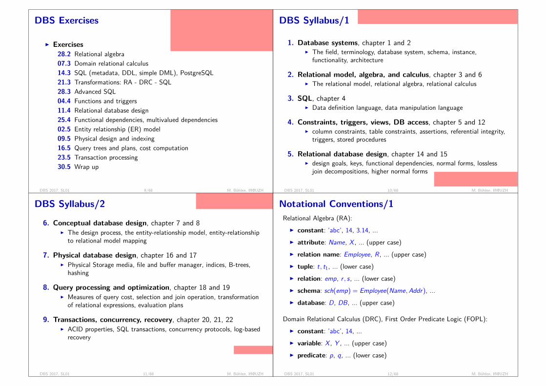
I I have been a database system person since more than 20 years.I My previous affiliations (and the first example of a database table):
AffiliationsStart End Institution Country1990 1994 ETH Zürich CH1994 1995 University of Arizona USA1995 2003 Aalborg University DK2003 2009 Free University of Bozen-Bolzano IT2009 now University of Zürich CH
expectation: no or little in terms of programming. basics in predicate logic.
DBS 2017, SL01 3/68 M. Böhlen, IfI@UZH
About the Database Systems Course
this week is not representative; overview; gets more technical and concrete.
I Slides can be accessed through the course web page:http://www.ifi.uzh.ch/dbtg/teaching/courses/DBS.html
I The slides are designed as a working script.I The textbook is Database Systems by Elmasri and Navathe.I Use the slides, and optionally the textbook, for preparation
throughout the semester.I During the lecture we will solve illustrative examples on the board.
Interaction during class is welcome.
I What is importantI Being able to apply your knowledge to relevant examples.I Being able to be precise about the key concepts of database systems.
DBS 2017, SL01 4/68 M. Böhlen, IfI@UZH
About Database Sytems @IfI
I Database Systems (DBS), Spring, 4th semester
I Praktikum Datenbanksysteme (PDBS), Fall, 5th semesterI Distributed Databases (DDBS), Fall even years, 5th semester
I Seminar Database Systems (SDBS), Spring, 6th or 8th semesterI XML und Datenbanken, (XMLDB), Spring, 6th or 8th semesterI Data Warehousing, Spring (DW), Spring even years, 8th semesterI Temporal and Spatial Data Management (TSDM), Fall odd
years, 9th semester
DBS 2017, SL01 5/68 M. Böhlen, IfI@UZH
Literature and Acknowledgments
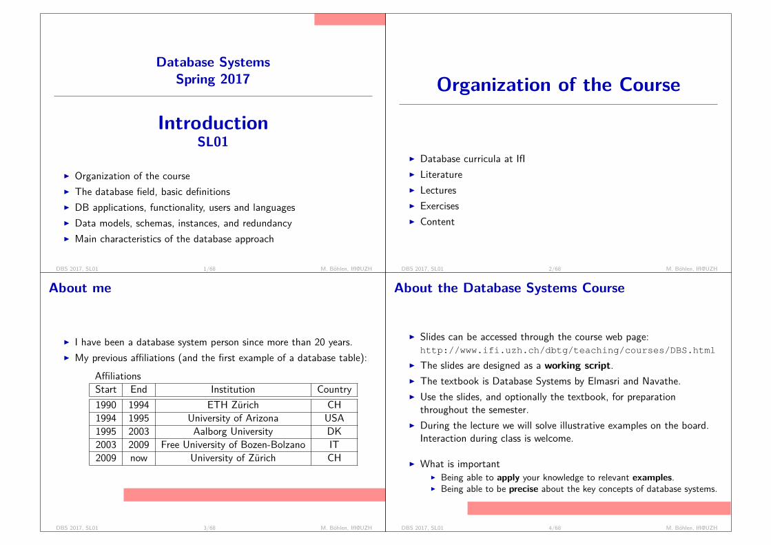
Reading List for SL01:I Database Systems, Chapters 1 and 2, Sixth
Edition, Ramez Elmasri and Shamkant B.Navathe, Pearson Education, 2010.
These slides were developed by:I Michael Böhlen, University of Zürich, SwitzerlandI Johann Gamper, Free University of Bozen-Bolzano, Italy
The slides are based on the following text books and associated material:I Database Systems, Sixth Edition, Ramez Elmasri and Shamkant B.
Navathe, Pearson Education, 2010.I A. Silberschatz, H. Korth, and S. Sudarshan: Database System
Concepts, McGraw Hill, 2006.
DBS 2017, SL01 6/68 M. Böhlen, IfI@UZH
DBS Course/1
I Lectures:I Tuesday 10:15-12:00 in BIN-0.K.02I Wednesday 12:15-13:45 in BIN-0.K.02
I The final exam is written and takes place Tuesday, June 20, 10:15 -12:00 (check official web pages for details).
I All written material (slides, exercises, exam) is in English.
The assessment consists of the completion of 9 out of 12 exercisesand the participation at the final exam. Both parts have to bepassed independently.
I Office hours after appointment with TAs (after exercise hour or byemail).
I There is no re-exam.
DBS 2017, SL01 7/68 M. Böhlen, IfI@UZH
DBS Course/2
I The weekly exercises are a crucial part of the course.I The exercises take place Tuesday 12:15-13:45. Start is February 28.
During the first week there are no exercises.I TAs: Oksana Dolmatova (English), Yvonne Mülle (German), Kevin
Wellenzohn (English).I Please sign up for the exercise groups by the end of this week by
filling the Doodle (cf. course web page). We will balance the loadacross groups.
I Hand in of the exercises is Tuesday 12:15 in the exercise room orbefore to TA directly.
I Exercises are only valid for the current year.
DBS 2017, SL01 8/68 M. Böhlen, IfI@UZH
DBS Exercises
Ausgabe 1. Uebung:I nächste WocheI Vorbesprechung der ÜbungI 1 Woche für BearbeitungI Besprechung der Lösung
I Exercises28.2 Relational algebra07.3 Domain relational calculus14.3 SQL (metadata, DDL, simple DML), PostgreSQL21.3 Transformations: RA - DRC - SQL28.3 Advanced SQL04.4 Functions and triggers11.4 Relational database design25.4 Functional dependencies, multivalued dependencies02.5 Entity relationship (ER) model09.5 Physical design and indexing16.5 Query trees and plans, cost computation23.5 Transaction processing30.5 Wrap up
DBS 2017, SL01 9/68 M. Böhlen, IfI@UZH
DBS Syllabus/1
bottom up. start with small well-defined pieces. bigger picture atthe end.
1. Database systems, chapter 1 and 2I The field, terminology, database system, schema, instance,
functionality, architecture
2. Relational model, algebra, and calculus, chapter 3 and 6I The relational model, relational algebra, relational calculus
3. SQL, chapter 4I Data definition language, data manipulation language
4. Constraints, triggers, views, DB access, chapter 5 and 12I column constraints, table constraints, assertions, referential integrity,
triggers, stored procedures
5. Relational database design, chapter 14 and 15I design goals, keys, functional dependencies, normal forms, lossless
join decompositions, higher normal forms
logical level (= relational model)
DBS 2017, SL01 10/68 M. Böhlen, IfI@UZH
DBS Syllabus/2
6. Conceptual database design, chapter 7 and 8I The design process, the entity-relationship model, entity-relationship
to relational model mapping
7. Physical database design, chapter 16 and 17I Physical Storage media, file and buffer manager, indices, B-trees,
hashing
8. Query processing and optimization, chapter 18 and 19I Measures of query cost, selection and join operation, transformation
of relational expressions, evaluation plans
9. Transactions, concurrency, recovery, chapter 20, 21, 22I ACID properties, SQL transactions, concurrency protocols, log-based
recovery
conceptual level (applicationsand users)
internal level
DBS 2017, SL01 11/68 M. Böhlen, IfI@UZH
Notational Conventions/1Relational Algebra (RA):
I constant: ’abc’, 14, 3.14, ...I attribute: Name, X , ... (upper case)I relation name: Employee, R, ... (upper case)I tuple: t, t1, ... (lower case)I relation: emp, r , s, ... (lower case)I schema: sch(emp) = Employee(Name, Addr), ...I database: D, DB, ... (upper case)
Domain Relational Calculus (DRC), First Order Predicate Logic (FOPL):I constant: ’abc’, 14, ...I variable: X , Y , ... (upper case)I predicate: p, q, ... (lower case)
DBS 2017, SL01 12/68 M. Böhlen, IfI@UZH
Notational Conventions/2
SQL:I constant: ’abc’, 14, ...I SQL keyword: SELECT, FROM, ... (all cap, blue, bold)I attribute: Name, Salary , ... (upper case)I table: r , dept, ... (lower case)
Entity Relationship Model (ER Model):I constant: ’abc’, 14, ...I attribute: Name, Gender , ... (green, upper case)I relationship: workFor , ... (red, lower case)I entity: Company , Emp, ... (blue, upper case)
DBS 2017, SL01 13/68 M. Böhlen, IfI@UZH
The Database Field
I Professional ResourcesI ProductsI Activities of Database PeopleI Basic Terminology and Definitions
DBS 2017, SL01 14/68 M. Böhlen, IfI@UZH
The Field/1
less than 20% acceptance rate; 600 submissions per year; 1-2years of work for 12 pages; 1-2 publ = PhD; more than 4publ = academic positions
I Conference PublicationsI SIGMOD/PODSI VLDBI ICDEI EDBT/ICDT
I Journal PublicationsI ACM Transaction on Database System (TODS)I The VLDB Journal (VLDBJ)I Information Systems (IS)I IEEE Transactions on Knowledge and Data Engineering (TKDE)
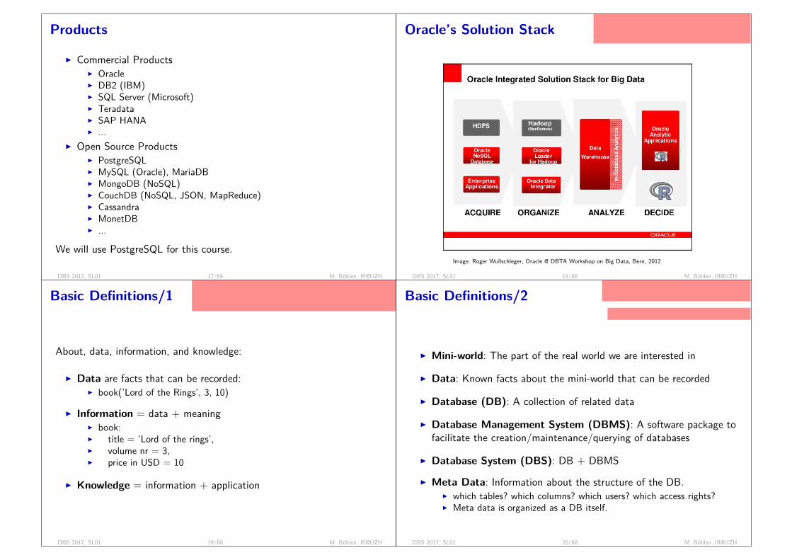
I DBLP Bibliography (Michael Ley, Uni Trier, Germany)I http://dblp.uni-trier.de/db/
I DBWorld mailing listI http://www.cs.wisc.edu/dbworld/
DBS 2017, SL01 15/68 M. Böhlen, IfI@UZH
The Field/2
DBS 2017, SL01 16/68 M. Böhlen, IfI@UZH
Products
I Commercial ProductsI OracleI DB2 (IBM)I SQL Server (Microsoft)I TeradataI SAP HANAI ...
I Open Source ProductsI PostgreSQLI MySQL (Oracle), MariaDBI MongoDB (NoSQL)I CouchDB (NoSQL, JSON, MapReduce)I CassandraI MonetDBI ...
We will use PostgreSQL for this course.
DBS 2017, SL01 17/68 M. Böhlen, IfI@UZH
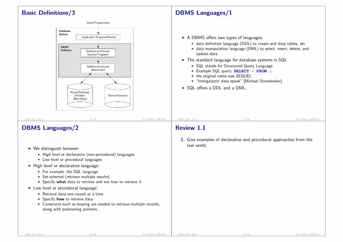
Oracle’s Solution Stack
x axis: data management –> data analysisy axis: distribution and heterogeneity0.5M CHF
Image: Roger Wullschleger, Oracle @ DBTA Workshop on Big Data, Bern, 2012
DBS 2017, SL01 18/68 M. Böhlen, IfI@UZH
Basic Definitions/1
dbs: general tools and techniques to process data; leavesemantics to applications; provide support to applicationsby processing data flexibly
About, data, information, and knowledge:
I Data are facts that can be recorded:I book(’Lord of the Rings’, 3, 10)
I Information = data + meaningI book:I title = ’Lord of the rings’,I volume nr = 3,I price in USD = 10
I Knowledge = information + application
DBS 2017, SL01 19/68 M. Böhlen, IfI@UZH
Basic Definitions/2
be precise (correct) about difference bet-ween db and dbms
facts: statements that are true or false
I Mini-world: The part of the real world we are interested in
I Data: Known facts about the mini-world that can be recorded
I Database (DB): A collection of related data
I Database Management System (DBMS): A software package tofacilitate the creation/maintenance/querying of databases
I Database System (DBS): DB + DBMS
I Meta Data: Information about the structure of the DB.I which tables? which columns? which users? which access rights?I Meta data is organized as a DB itself.
DBS 2017, SL01 20/68 M. Böhlen, IfI@UZH
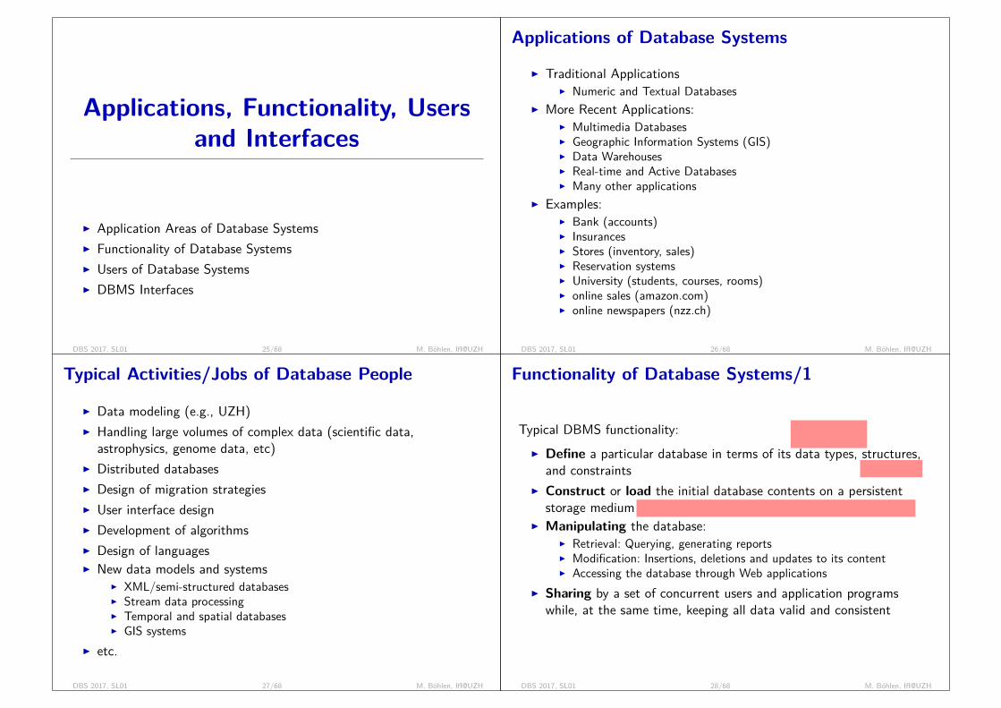
Basic Definitions/3
DBS 2017, SL01 21/68 M. Böhlen, IfI@UZH
DBMS Languages/1
I A DBMS offers two types of languages:I data definition language (DDL) to create and drop tables, etcI data manipulation language (DML) to select, insert, delete, and
update dataI The standard language for database systems is SQL
I SQL stands for Structured Query LanguageI Example SQL query: SELECT * FROM rI the original name was SEQUELI “Intergalactic data speak” [Michael Stonebraker].
I SQL offers a DDL and a DML.
DBS 2017, SL01 22/68 M. Böhlen, IfI@UZH
DBMS Languages/2
I We distinguish betweenI High level or declarative (non-procedural) languagesI Low level or procedural languages
I High level or declarative language:I For example, the SQL languageI Set-oriented (retrieve multiple results)I Specify what data to retrieve and not how to retrieve it
I Low level or procedural language:I Retrieve data one record at a timeI Specify how to retrieve dataI Constructs such as looping are needed to retrieve multiple records,
along with positioning pointers.
DBS 2017, SL01 23/68 M. Böhlen, IfI@UZH
Review 1.1
1. Give examples of declarative and procedural approaches from thereal world.
Procedural:cooking recipe: steps to cook a meal.
Python, C, Java, etc: program is sequence of steps.
Declarative:Search with Google: what to search and not how to search.
borrow a book from the uzh library: which book not how to find it.
SQL: what to compute not how to compute.
DBS 2017, SL01 24/68 M. Böhlen, IfI@UZH
Applications, Functionality, Usersand Interfaces
I Application Areas of Database SystemsI Functionality of Database SystemsI Users of Database SystemsI DBMS Interfaces
DBS 2017, SL01 25/68 M. Böhlen, IfI@UZH
Applications of Database Systems
I Traditional ApplicationsI Numeric and Textual Databases
I More Recent Applications:I Multimedia DatabasesI Geographic Information Systems (GIS)I Data WarehousesI Real-time and Active DatabasesI Many other applications
I Examples:I Bank (accounts)I InsurancesI Stores (inventory, sales)I Reservation systemsI University (students, courses, rooms)I online sales (amazon.com)I online newspapers (nzz.ch)
DBS 2017, SL01 26/68 M. Böhlen, IfI@UZH
Typical Activities/Jobs of Database People
I Data modeling (e.g., UZH)I Handling large volumes of complex data (scientific data,
astrophysics, genome data, etc)I Distributed databasesI Design of migration strategiesI User interface designI Development of algorithmsI Design of languagesI New data models and systems
I XML/semi-structured databasesI Stream data processingI Temporal and spatial databasesI GIS systems
I etc.
DBS 2017, SL01 27/68 M. Böhlen, IfI@UZH
Functionality of Database Systems/1
Typical DBMS functionality:I Define a particular database in terms of its data types, structures,
and constraints
integer, string,picture
tuple, table
I Construct or load the initial database contents on a persistentstorage medium
UBS, UZH, Swiss RE, Uni Spital, Google, Facebook, Twitter
I Manipulating the database:I Retrieval: Querying, generating reportsI Modification: Insertions, deletions and updates to its contentI Accessing the database through Web applications
I Sharing by a set of concurrent users and application programswhile, at the same time, keeping all data valid and consistent
DBS 2017, SL01 28/68 M. Böhlen, IfI@UZH
Functionality of Database Systems/2
Additional DBMS functionality:I Other features of DBMSs:
I Protection or security measures to prevent unauthorized accessI Active processing to take internal actions on dataI Presentation and visualization of dataI Maintaining the database and associated programs over the lifetime
of the database application (called database, software, and systemmaintenance)
DBS 2017, SL01 29/68 M. Böhlen, IfI@UZH
Users of Database Systems/1
Database users have very different tasks. There are those who use andcontrol the database content, and those who design, develop andmaintain database applications.
I Database administrators:I Responsible for authorizing access to the database, for coordinating
and monitoring its use, acquiring software and hardware resources,controlling its use and monitoring efficiency of operations.
I Database Designers:I Responsible to define the content, the structure, the constraints, and
functions or transactions against the database. They mustcommunicate with the end-users and understand their needs.
DBS 2017, SL01 30/68 M. Böhlen, IfI@UZH
Users of Database Systems/2
I End-users: They use the data for queries, reports and some of themupdate the database content. End-users can be categorized into:
I Casual: access database occasionally when neededI Naïve: they make up a large section of the end-user population.
I They use previously well-defined functions in the form of “cannedtransactions” against the database.
I Examples are bank-tellers or reservation clerks.I Sophisticated:
I These include business analysts, scientists, engineers, othersthoroughly familiar with the system capabilities.
I Many use tools in the form of software packages that work closelywith the stored database.
I Stand-alone:I Mostly maintain personal databases using ready-to-use packaged
applications.I An example is a tax program user that creates its own internal
database or a user that maintains an address book
DBS 2017, SL01 31/68 M. Böhlen, IfI@UZH
DBMS Interfaces/1
I User-friendly interfacesI Menu-based, forms-based, graphics-based, etc.
I Stand-alone query language interfacesI Example: Entering SQL queries at the DBMS interactive SQL
interface (e.g. psql in PostgreSQL, sqlplus in Oracle)I Program interfaces for embedding DML in programming languagesI Web Browser as an interfaceI Speech as Input and OutputI Parametric interfaces, e.g., bank tellers using function keys.I Interfaces for the DBA:
I Creating user accounts, granting authorizationsI Setting system parametersI Changing schemas or access paths
DBS 2017, SL01 32/68 M. Böhlen, IfI@UZH
DBMS Interfaces/2
I Programmer interfaces for embedding DML in programminglanguages:
I Embedded Approach:
move data from DB to application
embedded SQL (for C, C++, etc.)SQLJ (for Java)
I Procedure Call Approach:
move data from DB to application
JDBC for JavaODBC for other programming languages
Excel, R, ...
I Database Programming Language Approach:
move code from appl to DB
e.g., ORACLE has PL/SQL, a programming language based on SQL;language incorporates SQL and its data types as integral components
DBS 2017, SL01 33/68 M. Böhlen, IfI@UZH
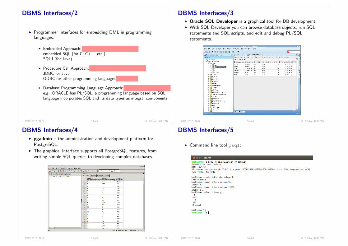
DBMS Interfaces/3I Oracle SQL Developer is a graphical tool for DB development.I With SQL Developer you can browse database objects, run SQL
statements and SQL scripts, and edit and debug PL/SQLstatements.
DBS 2017, SL01 34/68 M. Böhlen, IfI@UZH
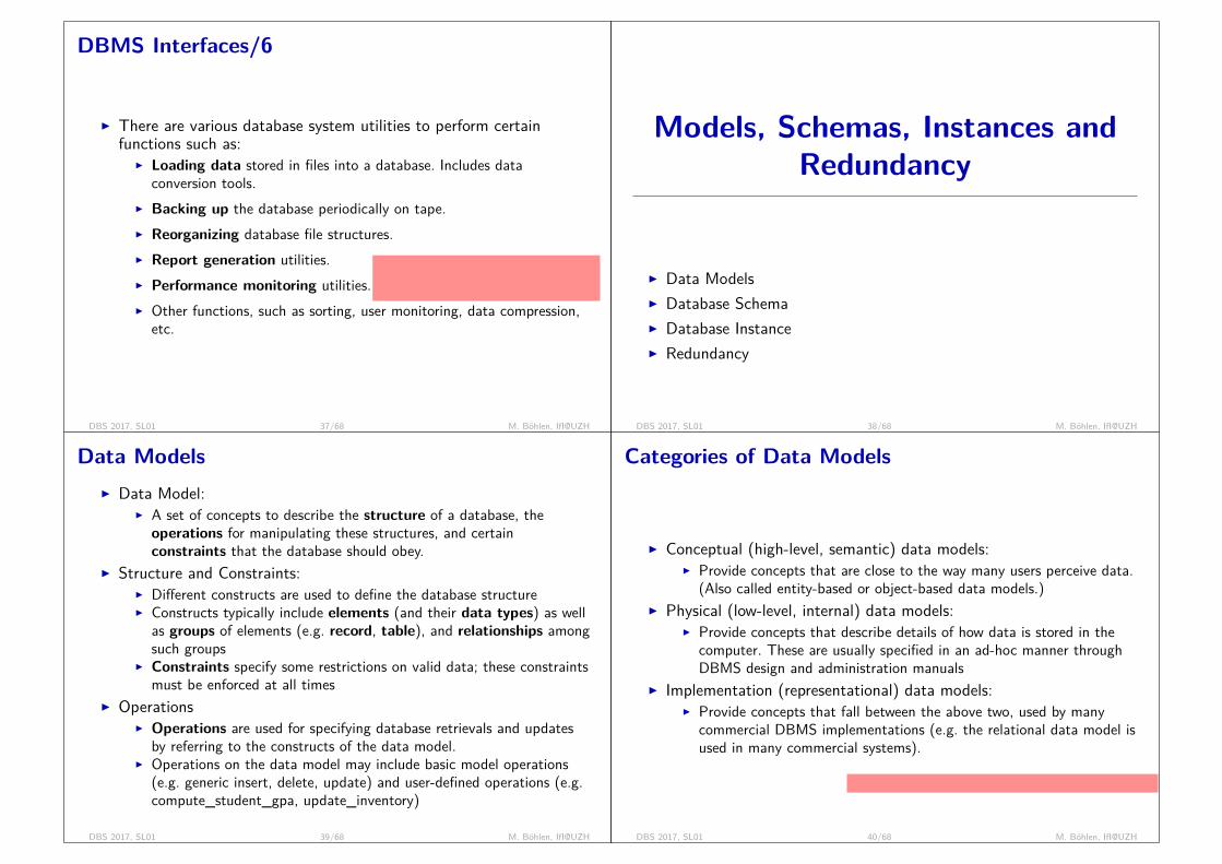
DBMS Interfaces/4I pgadmin is the administration and development platform for
PostgreSQL.I The graphical interface supports all PostgreSQL features, from
writing simple SQL queries to developing complex databases.
DBS 2017, SL01 35/68 M. Böhlen, IfI@UZH
DBMS Interfaces/5
I Command line tool psql:
DBS 2017, SL01 36/68 M. Böhlen, IfI@UZH
DBMS Interfaces/6
I There are various database system utilities to perform certainfunctions such as:
I Loading data stored in files into a database. Includes dataconversion tools.
I Backing up the database periodically on tape.I Reorganizing database file structures.I Report generation utilities.I Performance monitoring utilities.
Swiss Re: new DB2 release; changes toquery optimizer; increased query perfor-mance from 1 minute to 1 hour
I Other functions, such as sorting, user monitoring, data compression,etc.
DBS 2017, SL01 37/68 M. Böhlen, IfI@UZH
Models, Schemas, Instances andRedundancy
I Data ModelsI Database SchemaI Database InstanceI Redundancy
DBS 2017, SL01 38/68 M. Böhlen, IfI@UZH
Data ModelsI Data Model:
I A set of concepts to describe the structure of a database, theoperations for manipulating these structures, and certainconstraints that the database should obey.
I Structure and Constraints:I Different constructs are used to define the database structureI Constructs typically include elements (and their data types) as well
as groups of elements (e.g. record, table), and relationships amongsuch groups
I Constraints specify some restrictions on valid data; these constraintsmust be enforced at all times
I OperationsI Operations are used for specifying database retrievals and updates
by referring to the constructs of the data model.I Operations on the data model may include basic model operations
(e.g. generic insert, delete, update) and user-defined operations (e.g.compute_student_gpa, update_inventory)
DBS 2017, SL01 39/68 M. Böhlen, IfI@UZH
Categories of Data Models
Unterschiedliche Modelle für unterschiedliche Benutzer.
I Conceptual (high-level, semantic) data models:I Provide concepts that are close to the way many users perceive data.
(Also called entity-based or object-based data models.)I Physical (low-level, internal) data models:
I Provide concepts that describe details of how data is stored in thecomputer. These are usually specified in an ad-hoc manner throughDBMS design and administration manuals
I Implementation (representational) data models:I Provide concepts that fall between the above two, used by many
commercial DBMS implementations (e.g. the relational data model isused in many commercial systems).
DBS 2017, SL01 40/68 M. Böhlen, IfI@UZH
Database Schema
I Database Schema:I The description of a database.I Includes descriptions of the database structure, data types, and the
constraints on the database.I Schema Diagram:
I An illustrative display of (most aspects of) a database schema.I Schema Construct:
I A component of the schema or an object within the schema, e.g.,Student, Course.
I The database schema changes very infrequently.I Schema is also called intension.
DBS 2017, SL01 41/68 M. Böhlen, IfI@UZH
Database Instance
I Database Instance:I The actual data stored in a database at a particular moment in time.
This includes the collection of all the data in the database.I Also called database state (or occurrence or snapshot).I The term instance is also applied to individual database components,
e.g., record instance, table instance, entity instanceI Initial Database Instance: Refers to the database instance that is
initially loaded into the system.I Valid Database Instance: An instance that satisfies the structure
and constraints of the database.I The database instance changes every time the database is updated.I Instance is also called extension.
DBS 2017, SL01 42/68 M. Böhlen, IfI@UZH
Example of a Database DescriptionI Mini-world for the example:
I Part of a UNIVERSITY environment.I Some mini-world entities (an entity is a specific thing in the
mini-world):I STUDENTsI COURSEsI SECTIONs (of COURSEs)I DEPARTMENTsI INSTRUCTORs
I Some mini-world relationships (a relationship relates things of themini-world):
I SECTIONs are of specific COURSEsI STUDENTs take SECTIONsI COURSEs have prerequisiteI COURSE INSTRUCTORs teach SECTIONsI COURSEs are offered by DEPARTMENTsI STUDENTs major in DEPARTMENTs
DBS 2017, SL01 43/68 M. Böhlen, IfI@UZH
Example of a Database Schema
StudentName StudNr Class Major
CourseCourseName CourseNr CreditHours Department
PrerequisiteCourseNr PrerequisiteNr
SectionSectionID CourseNr Semester Year Instructor
GradeReportStudNr SectionId Grade
DBS 2017, SL01 44/68 M. Böhlen, IfI@UZH

Example of a Database Instance
good schema?
course(Course)CourseName CourseNr CreditHours Department
’Intro to Computer Science’ ’CS1310’ 4 ’CS’’Data Structures’ ’CS3320’ 4 CS
’Discrete Mathematics’ ’MATH2410’ 3 ’MATH’’Databases’ ’CS3360’ 3 ’CS’
section(Section)SectionID CourseNr Semester Year Instructor
85 ’MATH2410’ ’Fall’ 04 ’King’92 ’CS1310’ ’Fall’ 04 ’Anderson’102 ’CS3320’ ’Spring’ 05 ’Knuth’112 ’MATH2410’ ’Fall’ 05 ’Chang’119 ’CS1310’ ’Fall’ 05 ’Anderson’135 ’CS3380’ ’Fall’ 05 ’Stone’
gradeReport(GradeReport)StudNr SectionId Grade17 112 ’B’17 119 ’C’8 85 ’A’8 92 ’A’8 102 ’B’8 135 ’A’
prerequisite(Prerequisite)CourseNr PrerequisiteNr’CS3380’ ’CS3320’’CS3380’ ’MATH2410’’CS3320’ ’CS1310’
DBS 2017, SL01 45/68 M. Böhlen, IfI@UZH
Redundancy
I During the design of a database the number of tables and theirschemas must be determined.
I A key goal of database design is to avoid redundancy.
I Redundancy is present if information is stored multiple times.I Example of redundancy: storing the same address multiple timesI Redundancy leads to update anomalies and inconsistent data (e.g., a
person has multiple and partially invalid addresses)I The goal of database design, and specifically of database
normalization, is to eliminate redundancy.I The term controlled redundancy is used if duplication of
information is allowed and if the duplication is controlled by theDBMS.
DBS 2017, SL01 46/68 M. Böhlen, IfI@UZH
Review 1.2/1Consider the university database instance shown above.1. Explain why this schema contains redundancy.2. Give an example of a change that leads to update anomalies.3. Propose a modified schema that eliminates the redundancy.
1. In table Course the department appears redundantly in CourseNr (if in allcases the beginning of the course number is identical to the department).
2. Changing department from CS to CSSE: Anomaly/inconsistency occursif the course number is not changed as well.
if (’Data Structures’, ’CS3320’, 4, ’MATH’) is added then there is no redundancy sinceCourseNr and Dept get independent.
DBS 2017, SL01 47/68 M. Böhlen, IfI@UZH
Review 1.2/2
Solution 1 (drop department; suitable if no/few queries about department):coursesCourseName CourseNr CreditHours
... ’CS1310’ 4
... ’CS3320’ 4
... ’MATH2410’ 3
Solution 2 (split course nr; suitable for queries about department):coursesCourseName Dept CourseNr CreditH
... ’CS’ 1310 4
... ’CS’ 3320 4
... ’MATH’ 2410 3
prerequisiteCourseDept CourseNr PrecDept PrecNr
’CS’ 3380 ’CS’ 3320’CS’ 3380 ’MATH’ 2410’CS’ 3320 ’CS’ 1310
similar for section
should redundancy be eliminated? depends on risk of inconsistency and cost to avoid it.example: ISBN, AHV
DBS 2017, SL01 48/68 M. Böhlen, IfI@UZH

Main Characteristics of DatabaseSystems
I Three Schema ArchitectureI Data IndependenceI Main CharacteristicsI Advantages and Disadvantages of Database SystemsI History
DBS 2017, SL01 49/68 M. Böhlen, IfI@UZH
The ANSI/SPARC Three Schema Architecture/1
I Proposed to support DBMS characteristics of:I Data independenceI Multiple views of the data
I Not explicitly used in commercial DBMS products, but has beenuseful in explaining database system organization.
I Defines DBMS schemas at three levels:I Internal schema at the internal level to describe physical storage
structures and access paths (e.g indexes).I Typically uses a physical data model.
I Conceptual schema at the conceptual level to describe the structureand constraints for the whole database for a community of users.
I Uses a conceptual or an implementation data model.I External schemas at the external level to describe the various user
views.I Usually uses the same data model as the conceptual schema.
DBS 2017, SL01 50/68 M. Böhlen, IfI@UZH
The ANSI/SPARC Three Schema Architecture/2
I Mappings among schema levels are needed to transform requestsand data.
I Programs refer to an external schema, and are mapped by the DBMSto the internal schema for execution.
I Data extracted from the internal DBMS level is reformatted to matchthe user’s external view (e.g., formatting the results of an SQL queryfor display in a Web page)
DBS 2017, SL01 51/68 M. Böhlen, IfI@UZH
The ANSI/SPARC Three Schema Architecture/3
DBS 2017, SL01 52/68 M. Böhlen, IfI@UZH

Data Independence
uzh library: thematisch organisieren odernach Sprache organisieren (external viewcan be different)
uzh library: weiteres archiv
I Logical Data Independence:I The capacity to change the conceptual schema without having to
change the external schemas and their associated applicationprograms.
I Physical Data Independence:I The capacity to change the internal schema without having to change
the conceptual schema.I For example, the internal schema may be changed when certain file
structures are reorganized or new indexes are created to improvedatabase performance
I When a schema at a lower level is changed, only the mappingsbetween this schema and higher-level schemas need to be changedin a DBMS that fully supports data independence.
I The higher-level schemas themselves are unchanged.I Hence, the application programs need not be changed since they refer
to the external schemas.DBS 2017, SL01 53/68 M. Böhlen, IfI@UZH
Review 1.3
1. Give real world examples of data independence.
- Suche mit Google- Ausleihen eines Buches aus der UZH Bibliothek- Bewirtschaftung des Bankkontos- Zugriff auf Noten an der UZH
In all diesen Fällen- Verwendung der Daten ohne die Organisation der Daten zu kennen- hat die Anwendung keinen direkter Zugriff auf die Daten (accessthrough SQL only)
DBS 2017, SL01 54/68 M. Böhlen, IfI@UZH
Main Characteristics of Database Approach/1I Insulation between programs and data:
I Called data independence.I Allows changing data structures and storage organization without
having to change the DBMS access programs.I Control of redundancy:
I Database systems control (and minimize) redundancyI The control allows to avoid inconsistent data (happens if only one
copy is updated)I Data abstraction:
I A data model is used to hide storage details and present the userswith a conceptual view of the database.
I Programs refer to the data model constructs rather than data storagedetails
I Support of multiple views of the data:I Each user may see a different view of the database, which describes
only the data of interest to that user.
DBS 2017, SL01 55/68 M. Böhlen, IfI@UZH
Main Characteristics of Database Approach/2
I Sharing of data and multi-user transaction processing:I Allowing a set of concurrent users to retrieve from and to update the
database.I Concurrency control within the DBMS guarantees that each
transaction is correctly executed or abortedI Recovery subsystem ensures each completed transaction has its effect
permanently recorded in the databaseI OLTP (Online Transaction Processing) is a major part of database
applications. This allows hundreds of concurrent transactions toexecute per second.
I Self-describing nature of a database system:I A DBMS catalog stores the description of a particular database (e.g.
data types, data structures, and constraints)I The description is called metadata.I This allows the DBMS software to work with different database
applications.
DBS 2017, SL01 56/68 M. Böhlen, IfI@UZH
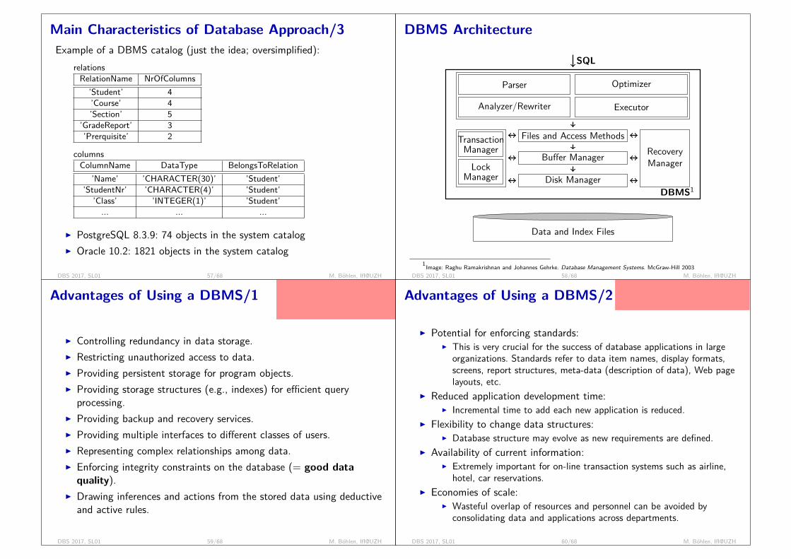
Main Characteristics of Database Approach/3Example of a DBMS catalog (just the idea; oversimplified):
relationsRelationName NrOfColumns
’Student’ 4’Course’ 4’Section’ 5
’GradeReport’ 3’Prerquisite’ 2
columnsColumnName DataType BelongsToRelation
’Name’ ’CHARACTER(30)’ ’Student’’StudentNr’ ’CHARACTER(4)’ ’Student’
’Class’ ’INTEGER(1)’ ’Student’... ... ...
I PostgreSQL 8.3.9: 74 objects in the system catalogI Oracle 10.2: 1821 objects in the system catalog
DBS 2017, SL01 57/68 M. Böhlen, IfI@UZH
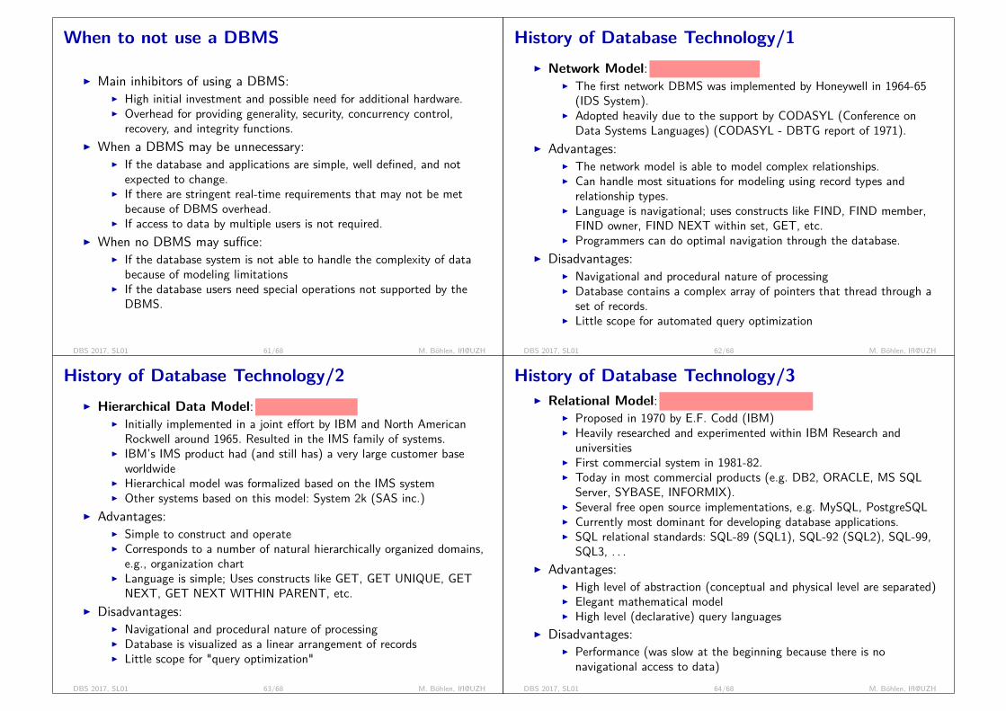
DBMS Architecture
SQL
DBMS1
Parser
Analyzer/Rewriter
Optimizer
Executor
Files and Access Methods
Buffer Manager
Disk Manager
RecoveryManager
TransactionManagerLock
Manager
Data and Index Files
1Image: Raghu Ramakrishnan and Johannes Gehrke. Database Management Systems. McGraw-Hill 2003DBS 2017, SL01 58/68 M. Böhlen, IfI@UZH
Advantages of Using a DBMS/1
data quality: kritisch für unter-nehmen. kann nicht/schwerkorrigiert werden. sicherstellungbei erfassung
I Controlling redundancy in data storage.I Restricting unauthorized access to data.I Providing persistent storage for program objects.I Providing storage structures (e.g., indexes) for efficient query
processing.I Providing backup and recovery services.I Providing multiple interfaces to different classes of users.I Representing complex relationships among data.I Enforcing integrity constraints on the database (= good dataquality).
I Drawing inferences and actions from the stored data using deductiveand active rules.
DBS 2017, SL01 59/68 M. Böhlen, IfI@UZH
Advantages of Using a DBMS/2
convinced? excited? dbms is not fan-cy sw. companies cannt do without.notizzettel, excel, dbs.
I Potential for enforcing standards:I This is very crucial for the success of database applications in large
organizations. Standards refer to data item names, display formats,screens, report structures, meta-data (description of data), Web pagelayouts, etc.
I Reduced application development time:I Incremental time to add each new application is reduced.
I Flexibility to change data structures:I Database structure may evolve as new requirements are defined.
I Availability of current information:I Extremely important for on-line transaction systems such as airline,
hotel, car reservations.I Economies of scale:
I Wasteful overlap of resources and personnel can be avoided byconsolidating data and applications across departments.
DBS 2017, SL01 60/68 M. Böhlen, IfI@UZH
When to not use a DBMS
I Main inhibitors of using a DBMS:I High initial investment and possible need for additional hardware.I Overhead for providing generality, security, concurrency control,
recovery, and integrity functions.I When a DBMS may be unnecessary:
I If the database and applications are simple, well defined, and notexpected to change.
I If there are stringent real-time requirements that may not be metbecause of DBMS overhead.
I If access to data by multiple users is not required.I When no DBMS may suffice:
I If the database system is not able to handle the complexity of databecause of modeling limitations
I If the database users need special operations not supported by theDBMS.
DBS 2017, SL01 61/68 M. Böhlen, IfI@UZH
History of Database Technology/1I Network Model:
= graph with pointers
I The first network DBMS was implemented by Honeywell in 1964-65(IDS System).
I Adopted heavily due to the support by CODASYL (Conference onData Systems Languages) (CODASYL - DBTG report of 1971).
I Advantages:I The network model is able to model complex relationships.I Can handle most situations for modeling using record types and
relationship types.I Language is navigational; uses constructs like FIND, FIND member,
FIND owner, FIND NEXT within set, GET, etc.I Programmers can do optimal navigation through the database.
I Disadvantages:I Navigational and procedural nature of processingI Database contains a complex array of pointers that thread through a
set of records.I Little scope for automated query optimization
DBS 2017, SL01 62/68 M. Böhlen, IfI@UZH
History of Database Technology/2I Hierarchical Data Model:
= tree with pointers
I Initially implemented in a joint effort by IBM and North AmericanRockwell around 1965. Resulted in the IMS family of systems.
I IBM’s IMS product had (and still has) a very large customer baseworldwide
I Hierarchical model was formalized based on the IMS systemI Other systems based on this model: System 2k (SAS inc.)
I Advantages:I Simple to construct and operateI Corresponds to a number of natural hierarchically organized domains,
e.g., organization chartI Language is simple; Uses constructs like GET, GET UNIQUE, GET
NEXT, GET NEXT WITHIN PARENT, etc.I Disadvantages:
I Navigational and procedural nature of processingI Database is visualized as a linear arrangement of recordsI Little scope for "query optimization"
DBS 2017, SL01 63/68 M. Böhlen, IfI@UZH
History of Database Technology/3I Relational Model:
= table with values (no pointers)
I Proposed in 1970 by E.F. Codd (IBM)I Heavily researched and experimented within IBM Research and
universitiesI First commercial system in 1981-82.I Today in most commercial products (e.g. DB2, ORACLE, MS SQL
Server, SYBASE, INFORMIX).I Several free open source implementations, e.g. MySQL, PostgreSQLI Currently most dominant for developing database applications.I SQL relational standards: SQL-89 (SQL1), SQL-92 (SQL2), SQL-99,
SQL3, . . .I Advantages:
I High level of abstraction (conceptual and physical level are separated)I Elegant mathematical modelI High level (declarative) query languages
I Disadvantages:I Performance (was slow at the beginning because there is no
navigational access to data)DBS 2017, SL01 64/68 M. Böhlen, IfI@UZH

History of Database Technology/4I Object-oriented models:
I Object-oriented database management systems (OODBMSs) wereintroduced in late 1980s and early 1990s to cater to the need ofcomplex data processing in CAD and other applications.
I OBJECTSTORE, VERSANT, GEMSTONE, O2, ORION, IRIS.I Object Database Standard: ODMG-93, ODMG-version 2.0,
ODMG-version 3.0.I Pure OODBMSs have disappeared. Many relational DBMSs have
incorporated object database concepts, leading to a new categorycalled object-relational DBMSs (ORDBMSs).
I Data on the web and E-commerce applications:I Web contains data in HTML with links among pages.I This has given rise to a new set of applications and E-commerce is
using standards like XML.I Script programming languages such as PHP and JavaScript allow
generation of dynamic Web pages that are partially generated from adatabase.
DBS 2017, SL01 65/68 M. Böhlen, IfI@UZH
History of Database Technology/5
I New functionality is being added to DBMSs in the following areas:I Scientific ApplicationsI XML (eXtensible Markup Language)I Image Storage and ManagementI Audio and Video Data ManagementI Data Warehousing and Data MiningI Spatial Data ManagementI Time Series and Historical Data ManagementI Key-value stores (NoSQL)
I The above gives rise to new research and development inincorporating new data types, complex data structures, newoperations and storage and indexing schemes in database systems.
DBS 2017, SL01 66/68 M. Böhlen, IfI@UZH
Summary/1I Data models, schemas, instances
I data model = structures + constraints + operationsI schema = intension; schema consists of structures and constraints;
schema changes infrequentlyI relation instance = relation = extension; relation instance is the
actual data that is compatible with the schema; changes oftenI Key characteristics of database systems
I controlled redundancy: database systems is aware of redundancyand provides support for updates that could violate the consistency ofthe data
I data independence: separation of program and data; makes itpossible to, e.g., reorganize internal schema without changingconceptual schema
I data abstraction: high level query language that is independent ofstorage structure
I data dictionary (metadata) that stores information about thedatabase itself (self-describing)
DBS 2017, SL01 67/68 M. Böhlen, IfI@UZH
Summary/2
I Three-Schema ArchitectureI multiple views of the dataI ANSI/SPARC three schema arcitectureI external, conceptual, and internal schema
I DBMS Languages and InterfacesI stand-alone command line interfaces: psql, sqlplus, ...I programming interfaces: ODBC, JDBCI database development tools: pgadmin, SQL developer
I Architectures and HistoryI networkI hierarchicalI relationalI object-oriented, object-relational
DBS 2017, SL01 68/68 M. Böhlen, IfI@UZH

Database SystemsSpring 2017
The Relational ModelSL02
Reviews: 14 17 23 35 38 43 55 75 78 82 85
I The Relational ModelI Basic Relational Algebra OperatorsI Additional Relational Algebra OperatorsI Extended Relational Algebra OperatorsI Modification of the DatabaseI Relational Calculus
DBS 2017, SL02 1/87 M. Böhlen, IfI@UZH
Literature and Acknowledgments
Reading List for SL02:I Database Systems, Chapters 3 and 6, Sixth Edition, Ramez Elmasri
and Shamkant B. Navathe, Pearson Education, 2010.
These slides were developed by:I Michael Böhlen, University of Zürich, SwitzerlandI Johann Gamper, Free University of Bozen-Bolzano, Italy
The slides are based on the following text books and associated material:I Fundamentals of Database Systems, Fourth Edition, Ramez Elmasri
and Shamkant B. Navathe, Pearson Addison Wesley, 2004.I A. Silberschatz, H. Korth, and S. Sudarshan: Database System
Concepts, McGraw Hill, 2006.
DBS 2017, SL02 2/87 M. Böhlen, IfI@UZH
The Relational Model
I schema, attribute, domain, tuple, relation, databaseI superkey, candidate key, primary keyI entity constraints, referential integrity
DBS 2017, SL02 3/87 M. Böhlen, IfI@UZH
The Relational Model/1
I The relational model is based on the concept of a relation.I A relation is a mathematical concept based on the ideas of sets.I The relational model was proposed by Codd from IBM Research in
the paper:I A Relational Model for Large Shared Data Banks, Communications of
the ACM, June 1970I The above paper caused a major revolution in the field of database
management and earned Codd the coveted ACM Turing Award.I The strength of the relational approach comes from the formal
foundation provided by the theory of relations.I In practice, there is a standard model based on SQL. There are
several important differences between the formal model and thepractical model, as we shall see.
DBS 2017, SL02 4/87 M. Böhlen, IfI@UZH
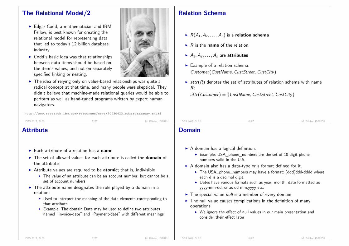
The Relational Model/2
I Edgar Codd, a mathematician and IBMFellow, is best known for creating therelational model for representing datathat led to today’s 12 billion databaseindustry.
I Codd’s basic idea was that relationshipsbetween data items should be based onthe item’s values, and not on separatelyspecified linking or nesting.
I The idea of relying only on value-based relationships was quite aradical concept at that time, and many people were skeptical. Theydidn’t believe that machine-made relational queries would be able toperform as well as hand-tuned programs written by expert humannavigators.
http://www.research.ibm.com/resources/news/20030423_edgarpassaway.shtml
DBS 2017, SL02 5/87 M. Böhlen, IfI@UZH
Relation Schema
I R(A1,A2, . . . ,An) is a relation schema
I R is the name of the relation.
I A1,A2, . . . ,An are attributes
I Example of a relation schema:Customer(CustName,CustStreet,CustCity)
I attr(R) denotes the set of attributes of relation schema with nameR:attr(Customer) = {CustName,CustStreet,CustCity}
DBS 2017, SL02 6/87 M. Böhlen, IfI@UZH
Attribute
I Each attribute of a relation has a nameI The set of allowed values for each attribute is called the domain of
the attributeI Attribute values are required to be atomic; that is, indivisible
I The value of an attribute can be an account number, but cannot be aset of account numbers
I The attribute name designates the role played by a domain in arelation:
I Used to interpret the meaning of the data elements corresponding tothat attribute
I Example: The domain Date may be used to define two attributesnamed “Invoice-date” and “Payment-date” with different meanings
DBS 2017, SL02 7/87 M. Böhlen, IfI@UZH
Domain
I A domain has a logical definition:I Example: USA_phone_numbers are the set of 10 digit phone
numbers valid in the U.S.I A domain also has a data-type or a format defined for it.
I The USA_phone_numbers may have a format: (ddd)ddd-dddd whereeach d is a decimal digit.
I Dates have various formats such as year, month, date formatted asyyyy-mm-dd, or as dd mm,yyyy etc.
I The special value null is a member of every domainI The null value causes complications in the definition of many
operationsI We ignore the effect of null values in our main presentation and
consider their effect later
DBS 2017, SL02 8/87 M. Böhlen, IfI@UZH

Tuple
alternative: (Name/’Adams’, Street/’Spring’, City/’Pittsfield’)SQL and DBMSs? support both; ordered if only values, unordered if attribute names
I A tuple is an ordered set (= list) of valuesI Angle brackets 〈...〉 are used as notation; sometimes regular
parentheses (...) are used as wellI Each value is derived from an appropriate domainI A customer tuple is a 3-tuple and would consist of three values, for
example:I (’Adams’, ’Spring’, ’Pittsfield’)
DBS 2017, SL02 9/87 M. Böhlen, IfI@UZH
Relational InstanceI r(R) denotes a relation (or relation instance) r on relation schema
with name RI Example: customer(Customer)I A relation instance is a subset of the Cartesian product of the
domains of its attributes. Thus, a relation is a set of n-tuples(a1, a2, . . . , an) where each ai ∈ Di
I Formally, given sets D1,D2, . . . ,Dn a relation r is a subset ofD1 × D2 × . . .× Dn
I Example:D1 = CustName = {’Jones’, ’Smith’, ’Curry’, ’Lindsay’, . . .}D2 = CustStreet = {’Main’, ’North’, ’Park’, . . .}D3 = CustCity = {’Harrison’, ’Rye’, ’Pittsfield’, . . .}r = { (’Jones’, ’Main’, ’Harrison’), (’Smith’, ’North’, ’Rye’),
(’Curry’, ’North’, ’Rye’), (’Lindsay’, ’Park’, ’Pittsfield’) }⊆ CustName × CustStreet × CustCity
DBS 2017, SL02 10/87 M. Böhlen, IfI@UZH
Example of a Relation
relation
tuples
attributes
relation name
account(Account)AccNr BranchName Balance’A-101’ ’Downtown’ 500’A-215’ ’Mianus’ 700’A-102’ ’Perryridge’ 400’A-305’ ’Round Hill’ 350’A-201’ ’Brighton’ 900’A-222’ ’Redwood’ 700’A-217’ ’Brighton’ 750
DBS 2017, SL02 11/87 M. Böhlen, IfI@UZH
The Customer Relation
customerCustName CustStreet CustCity’Adams’ ’Spring’ ’Pittsfield’’Brooks’ ’Senator’ ’Brooklyn’’Curry’ ’North’ ’Rye’’Glenn’ ’Sad Hill’ ’Woodside’’Green’ ’Walnut’ ’Stamford’’Hayes’ ’Main’ ’Harrison’’Johnson’ ’Alma’ ’Palo Alto’’Jones’ ’Main’ ’Harrison’’Lindsay’ ’Park’ ’Pittsfield’’Smith’ ’North’ ’Rye’’Turner’ ’Putnam’ ’Stamford’’Williams’ ’Nassau’ ’Princeton’
DBS 2017, SL02 12/87 M. Böhlen, IfI@UZH
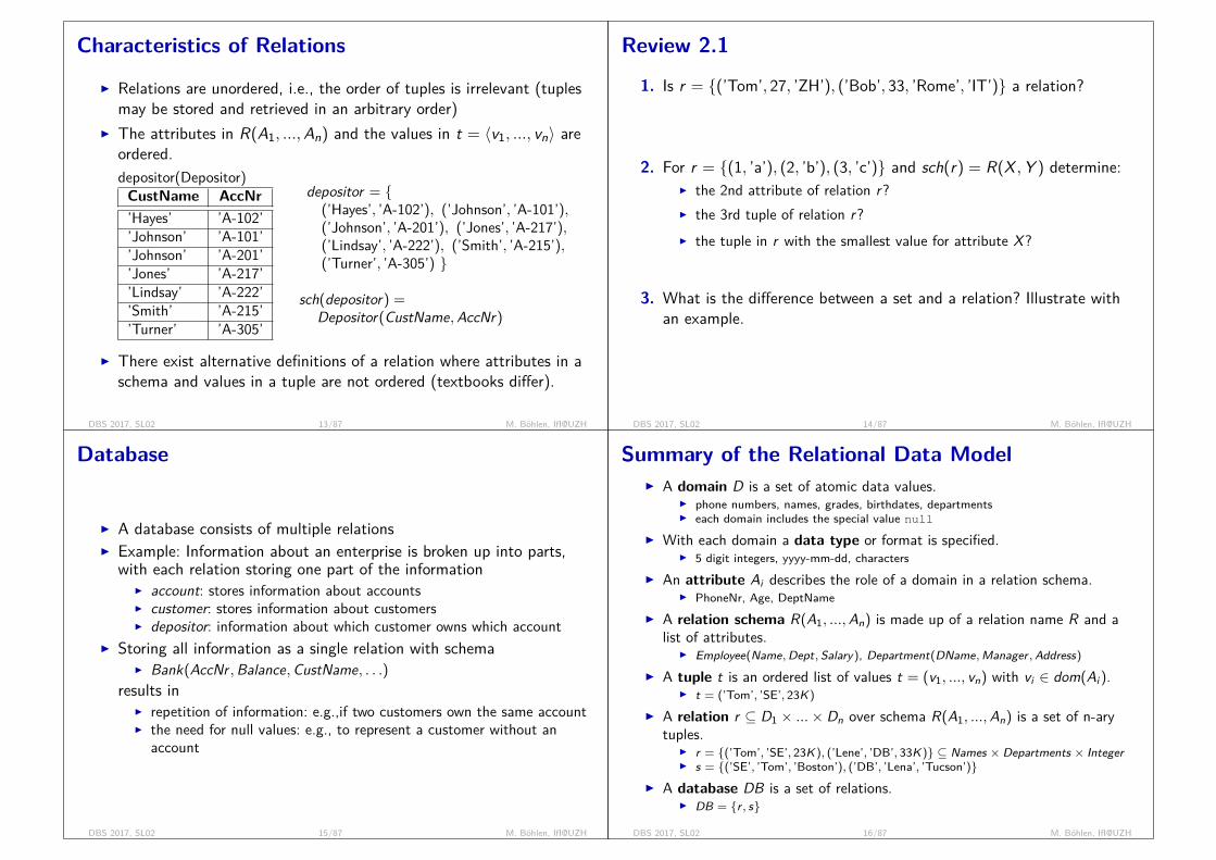
Characteristics of Relations
I Relations are unordered, i.e., the order of tuples is irrelevant (tuplesmay be stored and retrieved in an arbitrary order)
I The attributes in R(A1, ...,An) and the values in t = 〈v1, ..., vn〉 areordered.depositor(Depositor)CustName AccNr’Hayes’ ’A-102’’Johnson’ ’A-101’’Johnson’ ’A-201’’Jones’ ’A-217’’Lindsay’ ’A-222’’Smith’ ’A-215’’Turner’ ’A-305’
depositor = {(’Hayes’, ’A-102’), (’Johnson’, ’A-101’),(’Johnson’, ’A-201’), (’Jones’, ’A-217’),(’Lindsay’, ’A-222’), (’Smith’, ’A-215’),(’Turner’, ’A-305’) }
sch(depositor) =Depositor(CustName,AccNr)
I There exist alternative definitions of a relation where attributes in aschema and values in a tuple are not ordered (textbooks differ).
DBS 2017, SL02 13/87 M. Böhlen, IfI@UZH
Review 2.1
1. Is r = {(’Tom’, 27, ’ZH’), (’Bob’, 33, ’Rome’, ’IT’)} a relation?
No. Schemas of tuples are different. This is not allowed.
2. For r = {(1, ’a’), (2, ’b’), (3, ’c’)} and sch(r) = R(X ,Y ) determine:I the 2nd attribute of relation r?
Y.
I the 3rd tuple of relation r?
does not exist (no ordering)
I the tuple in r with the smallest value for attribute X?
(1,’a’)
3. What is the difference between a set and a relation? Illustrate withan example.
set: elements of a set can be anythingrelation: all elements are tuples with the same schemaX = {(’a’), ∗, {3}, (1, 2)} is a set but not a relation.
DBS 2017, SL02 14/87 M. Böhlen, IfI@UZH
Database
I A database consists of multiple relationsI Example: Information about an enterprise is broken up into parts,
with each relation storing one part of the informationI account: stores information about accountsI customer: stores information about customersI depositor: information about which customer owns which account
I Storing all information as a single relation with schemaI Bank(AccNr ,Balance,CustName, . . .)
results inI repetition of information: e.g.,if two customers own the same accountI the need for null values: e.g., to represent a customer without an
account
DBS 2017, SL02 15/87 M. Böhlen, IfI@UZH
Summary of the Relational Data ModelI A domain D is a set of atomic data values.
I phone numbers, names, grades, birthdates, departmentsI each domain includes the special value null
I With each domain a data type or format is specified.I 5 digit integers, yyyy-mm-dd, characters
I An attribute Ai describes the role of a domain in a relation schema.I PhoneNr, Age, DeptName
I A relation schema R(A1, ...,An) is made up of a relation name R and alist of attributes.
I Employee(Name,Dept, Salary), Department(DName,Manager ,Address)I A tuple t is an ordered list of values t = (v1, ..., vn) with vi ∈ dom(Ai).
I t = (’Tom’, ’SE’, 23K)I A relation r ⊆ D1 × ...× Dn over schema R(A1, ...,An) is a set of n-ary
tuples.I r = {(’Tom’, ’SE’, 23K), (’Lene’, ’DB’, 33K)} ⊆ Names × Departments × IntegerI s = {(’SE’, ’Tom’, ’Boston’), (’DB’, ’Lena’, ’Tucson’)}
I A database DB is a set of relations.I DB = {r , s}
DBS 2017, SL02 16/87 M. Böhlen, IfI@UZH
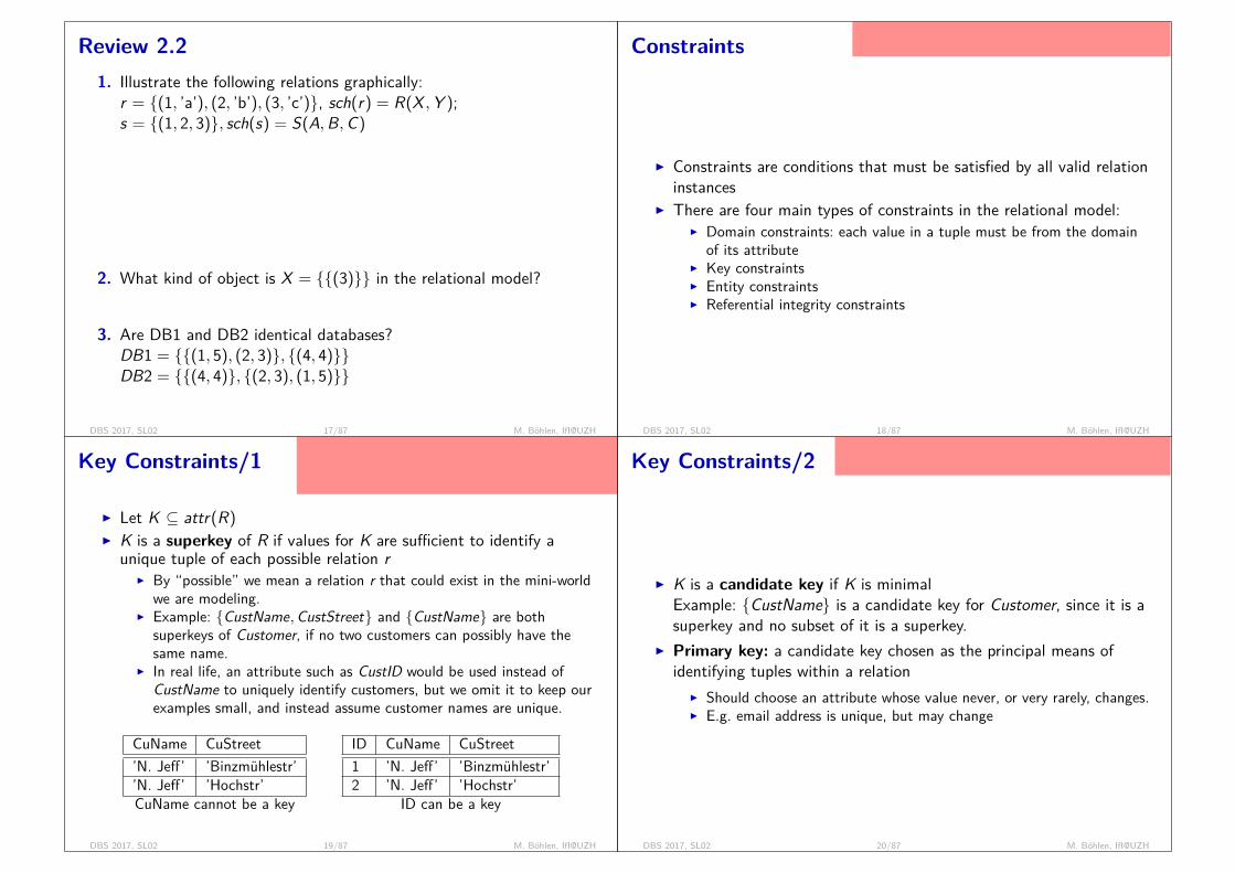
Review 2.21. Illustrate the following relations graphically:
r = {(1, ’a’), (2, ’b’), (3, ’c’)}, sch(r) = R(X ,Y );s = {(1, 2, 3)}, sch(s) = S(A,B,C)
r(R)X Y1 ’a’2 ’b’3 ’c’
s(S)A B C1 2 3
2. What kind of object is X = {{(3)}} in the relational model?
X is a database.
3. Are DB1 and DB2 identical databases?DB1 = {{(1, 5), (2, 3)}, {(4, 4)}}DB2 = {{(4, 4)}, {(2, 3), (1, 5)}}
Yes. Databases are sets of relations; relations are sets of tuples. Order is not relevant.
DBS 2017, SL02 17/87 M. Böhlen, IfI@UZH
Constraints
constraints restrict the content of tables; this guaranteesa good data quality!
I Constraints are conditions that must be satisfied by all valid relationinstances
I There are four main types of constraints in the relational model:I Domain constraints: each value in a tuple must be from the domain
of its attributeI Key constraintsI Entity constraintsI Referential integrity constraints
DBS 2017, SL02 18/87 M. Böhlen, IfI@UZH
Key Constraints/1
why are superkeys not very useful?superkeys are not minimal; SNr + Name + Gender + ...or AHVNr + Adr + FirstName + ... are superkeys.
I Let K ⊆ attr(R)I K is a superkey of R if values for K are sufficient to identify a
unique tuple of each possible relation rI By “possible” we mean a relation r that could exist in the mini-world
we are modeling.I Example: {CustName,CustStreet} and {CustName} are both
superkeys of Customer, if no two customers can possibly have thesame name.
I In real life, an attribute such as CustID would be used instead ofCustName to uniquely identify customers, but we omit it to keep ourexamples small, and instead assume customer names are unique.
CuName CuStreet’N. Jeff’ ’Binzmühlestr’’N. Jeff’ ’Hochstr’CuName cannot be a key
ID CuName CuStreet1 ’N. Jeff’ ’Binzmühlestr’2 ’N. Jeff’ ’Hochstr’
ID can be a key
DBS 2017, SL02 19/87 M. Böhlen, IfI@UZH
Key Constraints/2
candidate keys for students:SNr, AHVNr, LastName + FirstName + Address, email, ...
I K is a candidate key if K is minimalExample: {CustName} is a candidate key for Customer, since it is asuperkey and no subset of it is a superkey.
I Primary key: a candidate key chosen as the principal means ofidentifying tuples within a relation
I Should choose an attribute whose value never, or very rarely, changes.I E.g. email address is unique, but may change
DBS 2017, SL02 20/87 M. Böhlen, IfI@UZH
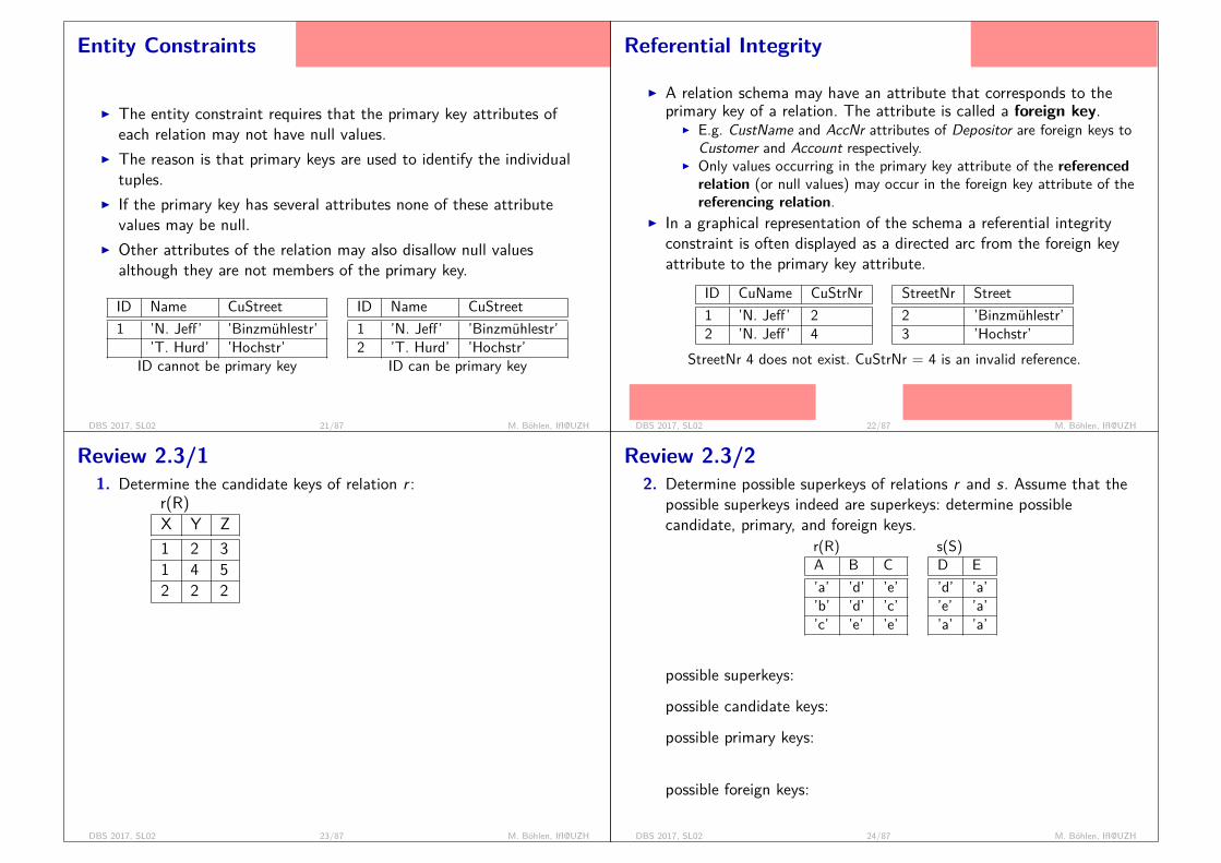
Entity Constraints
student without SNr; bank customer without accountnumber; employee without insurance nr; resident withouthealth insurance nr
I The entity constraint requires that the primary key attributes ofeach relation may not have null values.
I The reason is that primary keys are used to identify the individualtuples.
I If the primary key has several attributes none of these attributevalues may be null.
I Other attributes of the relation may also disallow null valuesalthough they are not members of the primary key.
ID Name CuStreet1 ’N. Jeff’ ’Binzmühlestr’
’T. Hurd’ ’Hochstr’ID cannot be primary key
ID Name CuStreet1 ’N. Jeff’ ’Binzmühlestr’2 ’T. Hurd’ ’Hochstr’
ID can be primary key
DBS 2017, SL02 21/87 M. Böhlen, IfI@UZH
Referential Integrity
Example of referential integrity:grades only for students with anS-number
I A relation schema may have an attribute that corresponds to theprimary key of a relation. The attribute is called a foreign key.
I E.g. CustName and AccNr attributes of Depositor are foreign keys toCustomer and Account respectively.
I Only values occurring in the primary key attribute of the referencedrelation (or null values) may occur in the foreign key attribute of thereferencing relation.
I In a graphical representation of the schema a referential integrityconstraint is often displayed as a directed arc from the foreign keyattribute to the primary key attribute.
ID CuName CuStrNr1 ’N. Jeff’ 22 ’N. Jeff’ 4
StreetNr Street2 ’Binzmühlestr’3 ’Hochstr’
StreetNr 4 does not exist. CuStrNr = 4 is an invalid reference.
foreign key (can only use knownstreets)
primary key (lists all possiblestreets)
DBS 2017, SL02 22/87 M. Böhlen, IfI@UZH
Review 2.3/11. Determine the candidate keys of relation r :
r(R)X Y Z1 2 31 4 52 2 2
X is not a key
Y is not a candidate key
Z could be a candidate key
XY could be a candidate key
Any superset of Z and XY could be a candidate key (only if nosubset is a candidate key)
DBS 2017, SL02 23/87 M. Böhlen, IfI@UZH
Review 2.3/22. Determine possible superkeys of relations r and s. Assume that the
possible superkeys indeed are superkeys: determine possiblecandidate, primary, and foreign keys.
r(R)A B C’a’ ’d’ ’e’’b’ ’d’ ’c’’c’ ’e’ ’e’
s(S)D E’d’ ’a’’e’ ’a’’a’ ’a’
possible superkeys:
A, AB, AC, ABC, BC, D, DE
possible candidate keys:
A, BC, D
possible primary keys:
A für R, D für S
possible foreign keys:
E with primary key A,B with primary key D,E with primary key D
DBS 2017, SL02 24/87 M. Böhlen, IfI@UZH
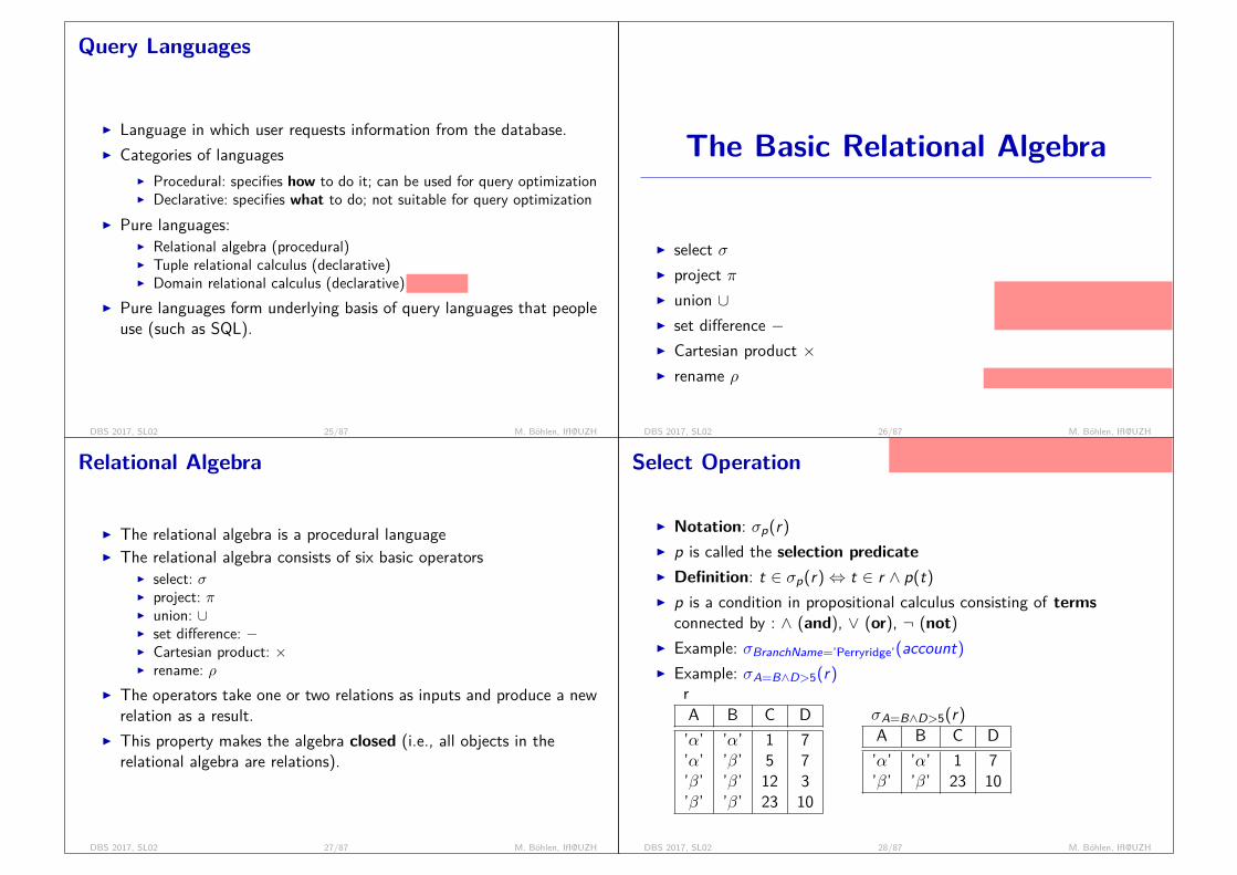
Query Languages
I Language in which user requests information from the database.I Categories of languages
I Procedural: specifies how to do it; can be used for query optimizationI Declarative: specifies what to do; not suitable for query optimization
I Pure languages:I Relational algebra (procedural)I Tuple relational calculus (declarative)I Domain relational calculus (declarative)
≈ FOPL
I Pure languages form underlying basis of query languages that peopleuse (such as SQL).
DBS 2017, SL02 25/87 M. Böhlen, IfI@UZH
goal is to calculate with rela-tions; equivalent to arithmeticoperations
1 table: Excel; > 1 table: DBMS
The Basic Relational Algebra
I select σI project πI union ∪I set difference −I Cartesian product ×I rename ρ
DBS 2017, SL02 26/87 M. Böhlen, IfI@UZH
Relational Algebra
I The relational algebra is a procedural languageI The relational algebra consists of six basic operators
I select: σI project: πI union: ∪I set difference: −I Cartesian product: ×I rename: ρ
I The operators take one or two relations as inputs and produce a newrelation as a result.
I This property makes the algebra closed (i.e., all objects in therelational algebra are relations).
DBS 2017, SL02 27/87 M. Böhlen, IfI@UZH
Select Operation
in examples identify:attribute name; string constant; number constant
I Notation: σp(r)I p is called the selection predicateI Definition: t ∈ σp(r)⇔ t ∈ r ∧ p(t)I p is a condition in propositional calculus consisting of terms
connected by : ∧ (and), ∨ (or), ¬ (not)I Example: σBranchName=’Perryridge’(account)I Example: σA=B∧D>5(r)
rA B C D’α’ ’α’ 1 7’α’ ’β’ 5 7’β’ ’β’ 12 3’β’ ’β’ 23 10
σA=B∧D>5(r)A B C D’α’ ’α’ 1 7’β’ ’β’ 23 10
DBS 2017, SL02 28/87 M. Böhlen, IfI@UZH
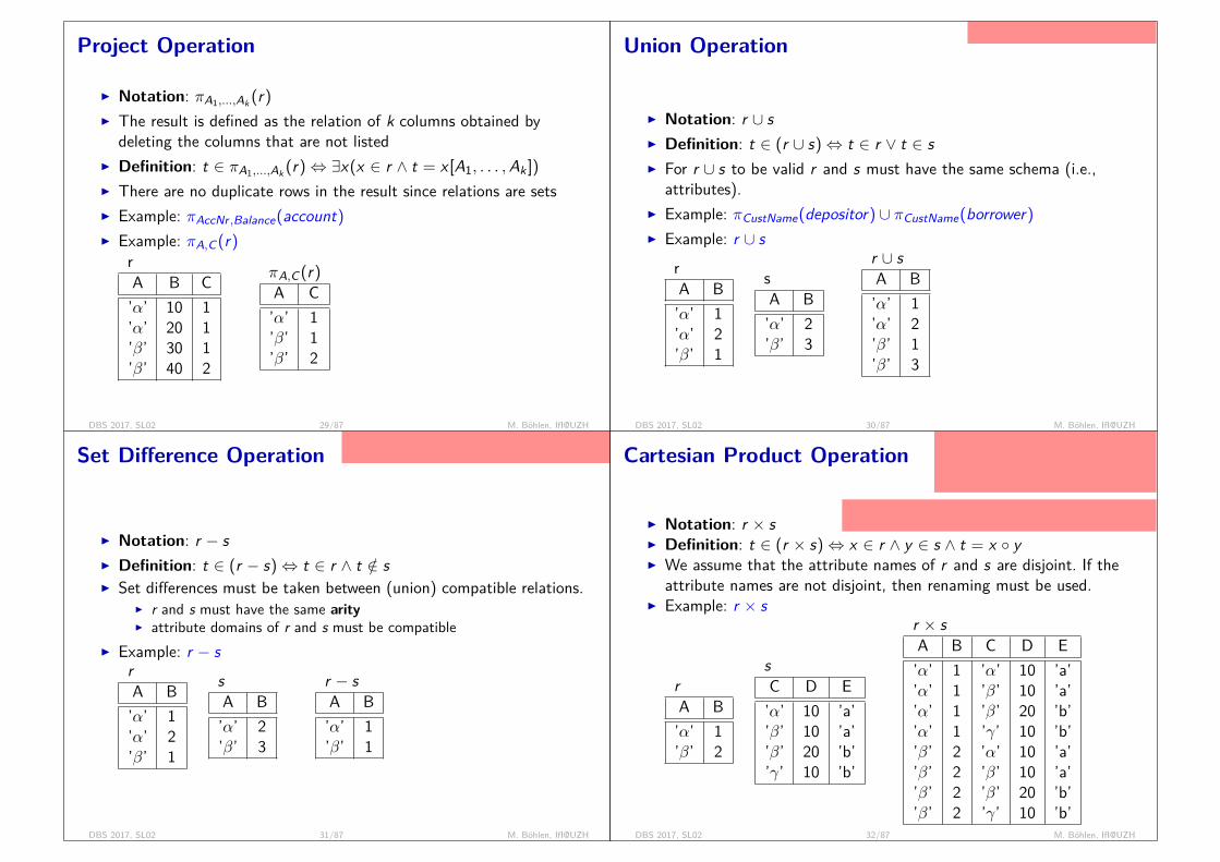
Project Operation
I Notation: πA1,...,Ak (r)I The result is defined as the relation of k columns obtained by
deleting the columns that are not listedI Definition: t ∈ πA1,...,Ak (r)⇔ ∃x(x ∈ r ∧ t = x [A1, . . . ,Ak ])I There are no duplicate rows in the result since relations are setsI Example: πAccNr ,Balance(account)I Example: πA,C (r)
rA B C’α’ 10 1’α’ 20 1’β’ 30 1’β’ 40 2
πA,C (r)A C’α’ 1’β’ 1’β’ 2
DBS 2017, SL02 29/87 M. Böhlen, IfI@UZH
Union Operation
no duplicates (relations are sets)
I Notation: r ∪ sI Definition: t ∈ (r ∪ s)⇔ t ∈ r ∨ t ∈ sI For r ∪ s to be valid r and s must have the same schema (i.e.,
attributes).I Example: πCustName(depositor) ∪ πCustName(borrower)I Example: r ∪ s
rA B’α’ 1’α’ 2’β’ 1
sA B’α’ 2’β’ 3
r ∪ sA B’α’ 1’α’ 2’β’ 1’β’ 3
DBS 2017, SL02 30/87 M. Böhlen, IfI@UZH
Set Difference Operation
note: union compatible + rename operations =same schema
I Notation: r − sI Definition: t ∈ (r − s)⇔ t ∈ r ∧ t /∈ sI Set differences must be taken between (union) compatible relations.
I r and s must have the same arityI attribute domains of r and s must be compatible
I Example: r − srA B’α’ 1’α’ 2’β’ 1
sA B’α’ 2’β’ 3
r − sA B’α’ 1’β’ 1
DBS 2017, SL02 31/87 M. Böhlen, IfI@UZH
Cartesian Product Operation
that’s it. such a language is relationally complete. roughlywhat dbms can do.
CP: generate all combinationsshow with r1, r2, s1, s2, ..., r1 ◦ s1, ...2 * 4 = 8meaningful use of CP requires practice
I Notation: r × sI Definition: t ∈ (r × s)⇔ x ∈ r ∧ y ∈ s ∧ t = x ◦ yI We assume that the attribute names of r and s are disjoint. If the
attribute names are not disjoint, then renaming must be used.I Example: r × s
rA B’α’ 1’β’ 2
sC D E’α’ 10 ’a’’β’ 10 ’a’’β’ 20 ’b’’γ’ 10 ’b’
r × sA B C D E’α’ 1 ’α’ 10 ’a’’α’ 1 ’β’ 10 ’a’’α’ 1 ’β’ 20 ’b’’α’ 1 ’γ’ 10 ’b’’β’ 2 ’α’ 10 ’a’’β’ 2 ’β’ 10 ’a’’β’ 2 ’β’ 20 ’b’’β’ 2 ’γ’ 10 ’b’
DBS 2017, SL02 32/87 M. Böhlen, IfI@UZH
Rename Operation
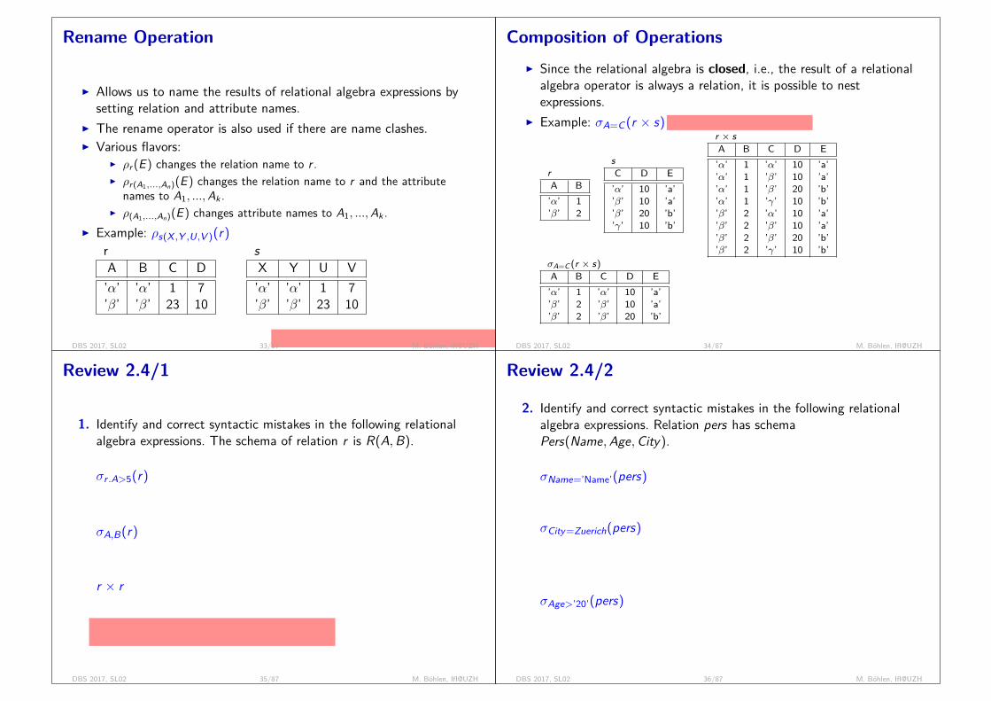
that’s it! use and work with it (requires practice)
I Allows us to name the results of relational algebra expressions bysetting relation and attribute names.
I The rename operator is also used if there are name clashes.I Various flavors:
I ρr (E ) changes the relation name to r .I ρr(A1,...,An)(E ) changes the relation name to r and the attribute
names to A1, ...,Ak .I ρ(A1,...,An)(E ) changes attribute names to A1, ...,Ak .
I Example: ρs(X ,Y ,U,V )(r)rA B C D’α’ ’α’ 1 7’β’ ’β’ 23 10
sX Y U V’α’ ’α’ 1 7’β’ ’β’ 23 10
DBS 2017, SL02 33/87 M. Böhlen, IfI@UZH
Composition of OperationsI Since the relational algebra is closed, i.e., the result of a relational
algebra operator is always a relation, it is possible to nestexpressions.
I Example: σA=C (r × s)
evaluate from inside to outside
rA B’α’ 1’β’ 2
sC D E’α’ 10 ’a’’β’ 10 ’a’’β’ 20 ’b’’γ’ 10 ’b’
r × sA B C D E’α’ 1 ’α’ 10 ’a’’α’ 1 ’β’ 10 ’a’’α’ 1 ’β’ 20 ’b’’α’ 1 ’γ’ 10 ’b’’β’ 2 ’α’ 10 ’a’’β’ 2 ’β’ 10 ’a’’β’ 2 ’β’ 20 ’b’’β’ 2 ’γ’ 10 ’b’
σA=C (r × s)A B C D E’α’ 1 ’α’ 10 ’a’’β’ 2 ’β’ 10 ’a’’β’ 2 ’β’ 20 ’b’
DBS 2017, SL02 34/87 M. Böhlen, IfI@UZH
Review 2.4/1
1. Identify and correct syntactic mistakes in the following relationalalgebra expressions. The schema of relation r is R(A,B).
σr .A>5(r)
r.A ist kein Attributname. Korrektur: σA>5(r)
σA,B(r)
Selektionsprädikat fehlt. Korrektur: πA,B(r)
r × r
Namenskonflikt. Korrektur: ρT (r × ρS[C ,D](r))ρS[C,D] required to resolve clash of attribute namesρT gives name to result relation is sometimes omitted
DBS 2017, SL02 35/87 M. Böhlen, IfI@UZH
Review 2.4/2
2. Identify and correct syntactic mistakes in the following relationalalgebra expressions. Relation pers has schemaPers(Name,Age,City).
σName=’Name’(pers)
OK.
σCity=Zuerich(pers)
Zuerich ist ein Wert und kein Attribut.Korrektur: σCity=’Zuerich’(pers)
σAge>’20’(pers)
Alter ist eine Zahl und keine Zeichenkette.Korrektur: σAlter>20(pers))
DBS 2017, SL02 36/87 M. Böhlen, IfI@UZH
Banking Example
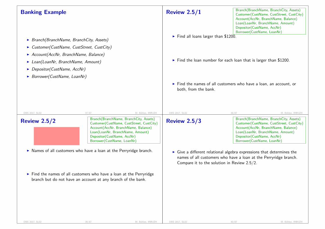
I Branch(BranchName, BranchCity, Assets)
Filiale
I Customer(CustName, CustStreet, CustCity)
Kunde
I Account(AccNr, BranchName, Balance)
Konten
I Loan(LoanNr, BranchName, Amount)
Kredite
I Depositor(CustName, AccNr)
Kontoinhaber
I Borrower(CustName, LoanNr)
Kreditnehmer
DBS 2017, SL02 37/87 M. Böhlen, IfI@UZH
Review 2.5/1 Branch(BranchName, BranchCity, Assets)Customer(CustName, CustStreet, CustCity)Account(AccNr, BranchName, Balance)Loan(LoanNr, BranchName, Amount)Depositor(CustName, AccNr)Borrower(CustName, LoanNr)
I Find all loans larger than $1200.
σAmount>1200(loan)
I Find the loan number for each loan that is larger than $1200.
πLoanNr (σAmount>1200(loan))
I Find the names of all customers who have a loan, an account, orboth, from the bank.
πCustName(borrower) ∪ πCustName(depositor)
DBS 2017, SL02 38/87 M. Böhlen, IfI@UZH
Review 2.5/2 Branch(BranchName, BranchCity, Assets)Customer(CustName, CustStreet, CustCity)Account(AccNr, BranchName, Balance)Loan(LoanNr, BranchName, Amount)Depositor(CustName, AccNr)Borrower(CustName, LoanNr)
loan1 D 502 P 203 D 10
borrowertom 1pam 2pam 3
I Names of all customers who have a loan at the Perryridge branch.
πCustName(σBranchName=‘Perryridge′(σLNr=LoanNr ((ρCustName,LNr (borrower))× loan)))
I Find the names of all customers who have a loan at the Perryridgebranch but do not have an account at any branch of the bank.
πCustName(σBranchName=’Perryridge’(σborrower .LoanNr=loan.LoanNr (borrower × loan)))−πCustName(depositor)
DBS 2017, SL02 39/87 M. Böhlen, IfI@UZH
Review 2.5/3 Branch(BranchName, BranchCity, Assets)Customer(CustName, CustStreet, CustCity)Account(AccNr, BranchName, Balance)Loan(LoanNr, BranchName, Amount)Depositor(CustName, AccNr)Borrower(CustName, LoanNr)
I Give a different relational algebra expressions that determines thenames of all customers who have a loan at the Perryridge branch.Compare it to the solution in Review 2.5/2.
πCustName(σLNr=LoanNr (σBranchName=‘Perryridge′(loan)×ρCustName,LNr (borrower)))
sol1: name of all customers, select perryridge customerssol2: select perryridge customers, determine their namesdbms makes this optimization; application cannot do it!
DBS 2017, SL02 40/87 M. Böhlen, IfI@UZH

Review 2.5/4 Branch(BranchName, BranchCity, Assets)Customer(CustName, CustStreet, CustCity)Account(AccNr, BranchName, Balance)Loan(LoanNr, BranchName, Amount)Depositor(CustName, AccNr)Borrower(CustName, LoanNr)
I Determine the largest account balance.
rephrase 1: all non-largest balances and subtract these from all balances.rephrase 2: all balances for which a larger exists and subtract these from all balances.
X123
×X123
=
X Y1 11 21 32 12 22 33 13 23 2
r − πX (σX<Y (r × ρ(Y )(r)))
DBS 2017, SL02 41/87 M. Böhlen, IfI@UZH
Formal Definition of Relational Algebra Expressions
I A basic expression in the relational algebra consists of either one ofthe following:
I A relation in the databaseI A constant relation (e.g., {(1, 2), (5, 3)})
I Let E1 and E2 be relational algebra expressions; the following are allrelational algebra expressions:
I E1 ∪ E2I E1 − E2I E1 × E2I σp(E1), p is a predicate on attributes in E1I πs(E1), s is a list consisting of some of the attributes in E1I ρx (E1), x is the new name for the result of E1
DBS 2017, SL02 42/87 M. Böhlen, IfI@UZH
Review 2.6/1Assume the following schemas:Train(TrainNr ,StartStat,EndStat)Link(FromStat,ToStat,TrainNr ,Departure,Arrival)
1. Sketch an instance of the database.
trainTrainNr StartStat EndStat’IC 706’ ’Zürich’ ’Geneva Airport’’IR 1798’ ’Zürich’ ’Basel’
linkFromStat ToStat TrainNr Departure Arrival’Zürich’ ’Lenzburg’ ’IC 706’ 5:21 5:40
’Lenzburg’ ’Aarau’ ’IC 706’ 5:40 5:47’Aarau’ ’Olten’ ’IC 706’ 5:49 5:58’Zürich’ ’Lenzburg’ ’IR 1798’ 0:08 0:27
DBS 2017, SL02 43/87 M. Böhlen, IfI@UZH
Review 2.6/2
2. Determine all direct connections (no change of train) from Zürich toOlten.
πFromStat,B,TrainNr ,Departure,E (σTrainNr=C∧Departure<D(
σFromStat=‘Zuerich‘(link) ×σB=‘Olten‘(ρ(A,B,C ,D,E)(link))))
ZH - Lenzburg - Aarau - OltenLangenthal - Olten - Aarau - Lenzburg - ZH - Flughafen
DBS 2017, SL02 44/87 M. Böhlen, IfI@UZH
Additional Relational AlgebraOperators
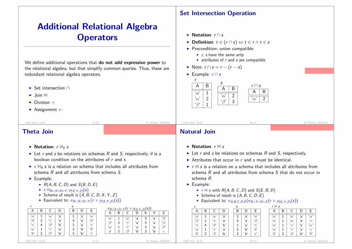
We define additional operations that do not add expressive power tothe relational algebra, but that simplify common queries. Thus, these areredundant relational algebra operators.
I Set intersection ∩I Join 1
I Division ÷I Assignment ←
DBS 2017, SL02 45/87 M. Böhlen, IfI@UZH
Set Intersection Operation
Venn diagramm
I Notation: r ∩ sI Definition: t ∈ (r ∩ s)⇔ t ∈ r ∧ t ∈ sI Precondition: union compatible
I r, s have the same arityI attributes of r and s are compatible
I Note: r ∩ s = r − (r − s)I Example: r ∩ s
rA B’α’ 1’α’ 2’β’ 1
sA B’α’ 2’β’ 3
r ∩ sA B’α’ 2
DBS 2017, SL02 46/87 M. Böhlen, IfI@UZH
Theta Join
in contrast to CP not all combinations.requires unique attr names to avoid clashes.
I Notation: r 1θ sI Let r and s be relations on schemas R and S, respectively. θ is a
boolean condition on the attributes of r and s.I r 1θ s is a relation on schema that includes all attributes from
schema R and all attributes from schema S.I Example:
I R(A,B,C ,D) and S(B,D,E )I r 1B<X∧D=Y ρ(X ,Y ,Z)(s)I Schema of result is (A,B,C ,D,X ,Y ,Z )I Equivalent to: σB<X∧D=Y (r × ρ(X ,Y ,Z)(s))
rA B C D’α’ 1 ’α’ ’a’’β’ 2 ’γ’ ’a’’γ’ 4 ’β’ ’b’’α’ 1 ’γ’ ’a’’δ’ 2 ’β’ ’b’
sB D E1 ’a’ ’α’3 ’a’ ’β’1 ’a’ ’γ’2 ’b’ ’δ’3 ’b’ ’ε’
σB<X∧D=Y (r × ρ(X ,Y ,Z)(s))A B C D X Y Z’α’ 1 ’α’ ’a’ 3 ’a’ ’β’’β’ 2 ’γ’ ’a’ 3 ’a’ ’β’’α’ 1 ’γ’ ’a’ 3 ’a’ ’β’δ 2 ’β’ ’b’ 3 ’b’ ε
DBS 2017, SL02 47/87 M. Böhlen, IfI@UZH
Natural Join
NJ requires common attribute names.
I Notation: r 1 sI Let r and s be relations on schemas R and S, respectively.I Attributes that occur in r and s must be identical.I r 1 s is a relation on a schema that includes all attributes from
schema R and all attributes from schema S that do not occur inschema R.
I Example:I r 1 s with R(A,B,C ,D) and S(E ,B,D)I Schema of result is (A,B,C ,D,E )I Equivalent to: πA,B,C ,D,E (σB=Y∧D=Z (r × ρ(E ,Y ,Z)(s))
rA B C D’α’ 1 ’α’ ’a’’β’ 2 ’γ’ ’a’’γ’ 4 ’β’ ’b’’α’ 1 ’γ’ ’a’’δ’ 2 ’β’ ’b’
sB D E1 ’a’ ’α’3 ’a’ ’β’1 ’a’ ’γ’2 ’b’ ’δ’3 ’b’ ’ε’
r 1 sA B C D E’α’ 1 ’α’ ’a’ ’α’’α’ 1 ’α’ ’a’ ’γ’’α’ 1 ’γ’ ’a’ ’α’’α’ 1 ’γ’ ’a’ ’γ’’δ’ 2 ’β’ ’b’ ’δ’
DBS 2017, SL02 48/87 M. Böhlen, IfI@UZH
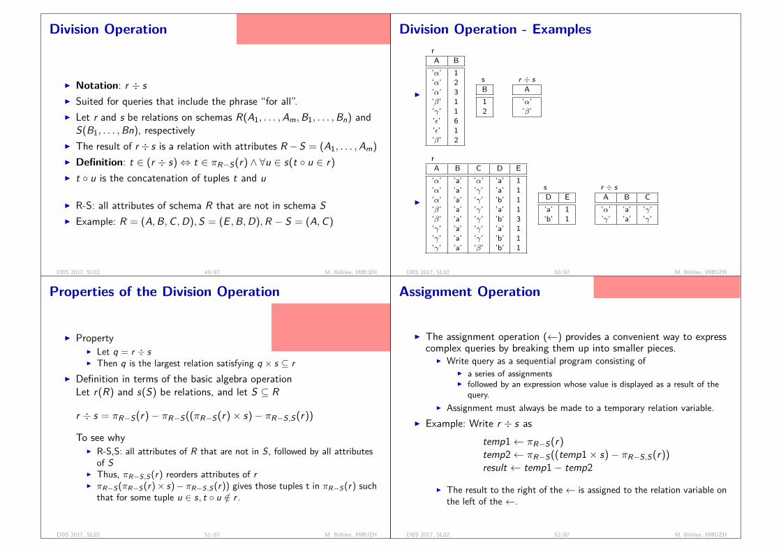
Division Operation
- students who passed all exams- persons who satisfy all requirements- countries where all languages are spoken
I Notation: r ÷ sI Suited for queries that include the phrase “for all”.I Let r and s be relations on schemas R(A1, . . . ,Am,B1, . . . ,Bn) and
S(B1, . . . ,Bn), respectivelyI The result of r ÷ s is a relation with attributes R−S = (A1, . . . ,Am)I Definition: t ∈ (r ÷ s)⇔ t ∈ πR−S(r) ∧ ∀u ∈ s(t ◦ u ∈ r)I t ◦ u is the concatenation of tuples t and u
I R-S: all attributes of schema R that are not in schema SI Example: R = (A,B,C ,D), S = (E ,B,D),R − S = (A,C)
DBS 2017, SL02 49/87 M. Böhlen, IfI@UZH
Division Operation - Examples
I
rA B’α’ 1’α’ 2’α’ 3’β’ 1’γ’ 1’ε’ 6’ε’ 1’β’ 2
sB12
r ÷ sA’α’’β’
I
rA B C D E’α’ ’a’ ’α’ ’a’ 1’α’ ’a’ ’γ’ ’a’ 1’α’ ’a’ ’γ’ ’b’ 1’β’ ’a’ ’γ’ ’a’ 1’β’ ’a’ ’γ’ ’b’ 3’γ’ ’a’ ’γ’ ’a’ 1’γ’ ’a’ ’γ’ ’b’ 1’γ’ ’a’ ’β’ ’b’ 1
sD E’a’ 1’b’ 1
r ÷ sA B C’α’ ’a’ ’γ’’γ’ ’a’ ’γ’
DBS 2017, SL02 50/87 M. Böhlen, IfI@UZH
Properties of the Division Operation
all combinationsexisting combinationsdesired combinations of r and sexisting combinations of r and smissing combinations of r and s
I PropertyI Let q = r ÷ sI Then q is the largest relation satisfying q × s ⊆ r
I Definition in terms of the basic algebra operationLet r(R) and s(S) be relations, and let S ⊆ R
r ÷ s = πR−S(r)− πR−S((πR−S(r)× s)− πR−S,S(r))
To see whyI R-S,S: all attributes of R that are not in S, followed by all attributes
of SI Thus, πR−S,S(r) reorders attributes of rI πR−S(πR−S(r)× s)− πR−S,S(r)) gives those tuples t in πR−S(r) such
that for some tuple u ∈ s, t ◦ u /∈ r .
DBS 2017, SL02 51/87 M. Böhlen, IfI@UZH
Assignment Operation
use assignment to break up complex ex-pressions into readable pieces
I The assignment operation (←) provides a convenient way to expresscomplex queries by breaking them up into smaller pieces.
I Write query as a sequential program consisting ofI a series of assignmentsI followed by an expression whose value is displayed as a result of the
query.I Assignment must always be made to a temporary relation variable.
I Example: Write r ÷ s astemp1← πR−S(r)temp2← πR−S((temp1× s)− πR−S,S(r))result ← temp1− temp2
I The result to the right of the ← is assigned to the relation variable onthe left of the ←.
DBS 2017, SL02 52/87 M. Böhlen, IfI@UZH
Bank Example Queries/1 Branch(BranchName, BranchCity, Assets)Customer(CustName, CustStreet, CustCity)Account(AccNr, BranchName, Balance)Loan(LoanNr, BranchName, Amount)Depositor(CustName, AccNr)Borrower(CustName, LoanNr)
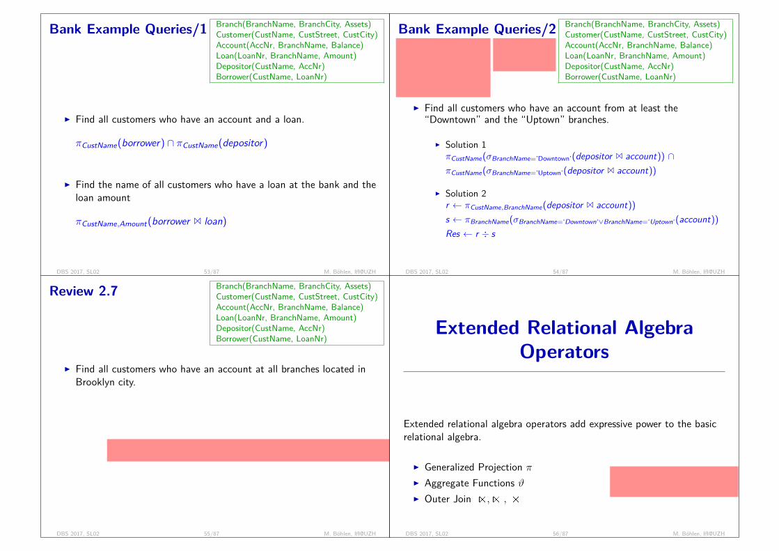
I Find all customers who have an account and a loan.
πCustName(borrower) ∩ πCustName(depositor)
I Find the name of all customers who have a loan at the bank and theloan amount
πCustName,Amount(borrower 1 loan)
DBS 2017, SL02 53/87 M. Böhlen, IfI@UZH
Bank Example Queries/2 Branch(BranchName, BranchCity, Assets)Customer(CustName, CustStreet, CustCity)Account(AccNr, BranchName, Balance)Loan(LoanNr, BranchName, Amount)Depositor(CustName, AccNr)Borrower(CustName, LoanNr)
r’Tom’ ’Uptown’’Tom’ ’Downtown’’Tom’ ’Perryridge’’Pam’ ’Uptown’’Pam’ ’Perryridge’
s’Uptown’
’Downtown’
I Find all customers who have an account from at least the“Downtown” and the “Uptown” branches.
I Solution 1πCustName(σBranchName=’Downtown’(depositor 1 account)) ∩πCustName(σBranchName=’Uptown’(depositor 1 account))
I Solution 2r ← πCustName,BranchName(depositor 1 account))s ← πBranchName(σBranchName=‘Downtown‘∨BranchName=‘Uptown‘(account))Res ← r ÷ s
DBS 2017, SL02 54/87 M. Böhlen, IfI@UZH
Review 2.7 Branch(BranchName, BranchCity, Assets)Customer(CustName, CustStreet, CustCity)Account(AccNr, BranchName, Balance)Loan(LoanNr, BranchName, Amount)Depositor(CustName, AccNr)Borrower(CustName, LoanNr)
I Find all customers who have an account at all branches located inBrooklyn city.
πCustName,BranchName(depositor 1 account))÷πBranchName(σBranchCity=‘Brooklyn‘(branch))
“all branches”: we do not know constants (all branch names); therefore we mustcompute them and use a division
DBS 2017, SL02 55/87 M. Böhlen, IfI@UZH
Extended Relational AlgebraOperators
null valuesfunctions (+, *, length, ...)aggregates are not part of core RA
Extended relational algebra operators add expressive power to the basicrelational algebra.
I Generalized Projection πI Aggregate Functions ϑI Outer Join d|><| , |><|d , d|><|d
DBS 2017, SL02 56/87 M. Böhlen, IfI@UZH
Generalized Projection
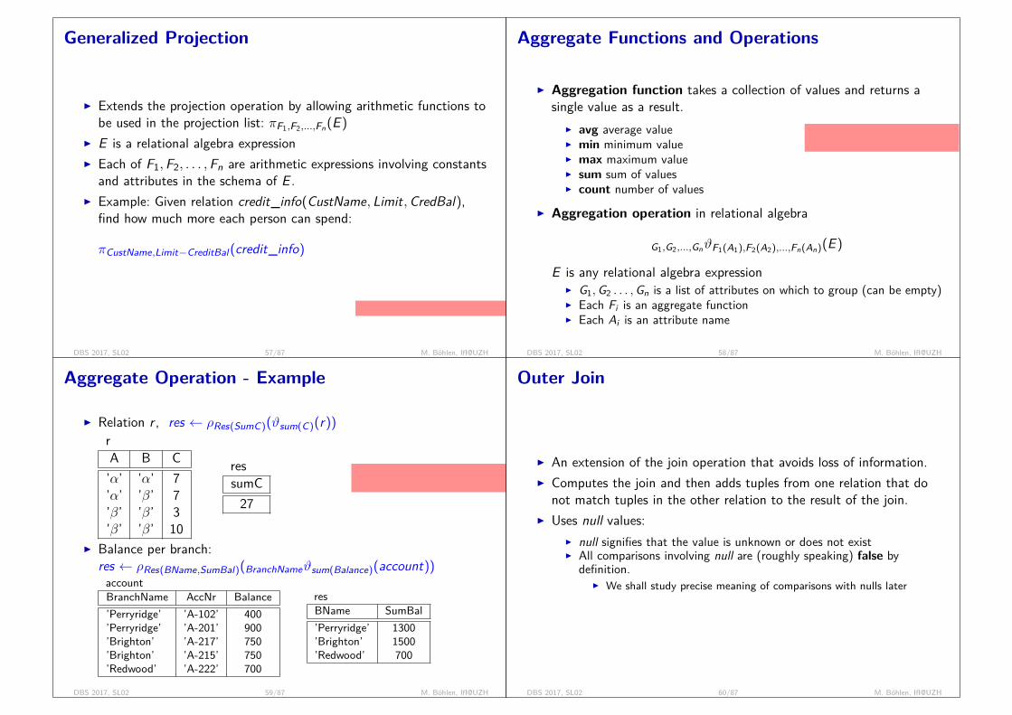
I Extends the projection operation by allowing arithmetic functions tobe used in the projection list: πF1,F2,...,Fn(E )
I E is a relational algebra expressionI Each of F1,F2, . . . ,Fn are arithmetic expressions involving constants
and attributes in the schema of E .I Example: Given relation credit_info(CustName, Limit,CredBal),
find how much more each person can spend:
πCustName,Limit−CreditBal(credit_info)
function: Limit - CreditBalance
DBS 2017, SL02 57/87 M. Böhlen, IfI@UZH
Aggregate Functions and Operations
avg, sum, count. initialized to 0;min, max: initialized to NULL
I Aggregation function takes a collection of values and returns asingle value as a result.
I avg average valueI min minimum valueI max maximum valueI sum sum of valuesI count number of values
I Aggregation operation in relational algebra
G1,G2,...,GnϑF1(A1),F2(A2),...,Fn(An)(E )
E is any relational algebra expressionI G1,G2 . . . ,Gn is a list of attributes on which to group (can be empty)I Each Fi is an aggregate functionI Each Ai is an attribute name
DBS 2017, SL02 58/87 M. Böhlen, IfI@UZH
Aggregate Operation - Example
duplicates are relevant for aggre-gate functions.
I Relation r , res ← ρRes(SumC)(ϑsum(C)(r))rA B C’α’ ’α’ 7’α’ ’β’ 7’β’ ’β’ 3’β’ ’β’ 10
ressumC27
I Balance per branch:res ← ρRes(BName,SumBal)(BranchNameϑsum(Balance)(account))
accountBranchName AccNr Balance’Perryridge’ ’A-102’ 400’Perryridge’ ’A-201’ 900’Brighton’ ’A-217’ 750’Brighton’ ’A-215’ 750’Redwood’ ’A-222’ 700
resBName SumBal’Perryridge’ 1300’Brighton’ 1500’Redwood’ 700
DBS 2017, SL02 59/87 M. Böhlen, IfI@UZH
Outer Join
I An extension of the join operation that avoids loss of information.I Computes the join and then adds tuples from one relation that do
not match tuples in the other relation to the result of the join.I Uses null values:
I null signifies that the value is unknown or does not existI All comparisons involving null are (roughly speaking) false by
definition.I We shall study precise meaning of comparisons with nulls later
DBS 2017, SL02 60/87 M. Böhlen, IfI@UZH
Outer Join Example/1
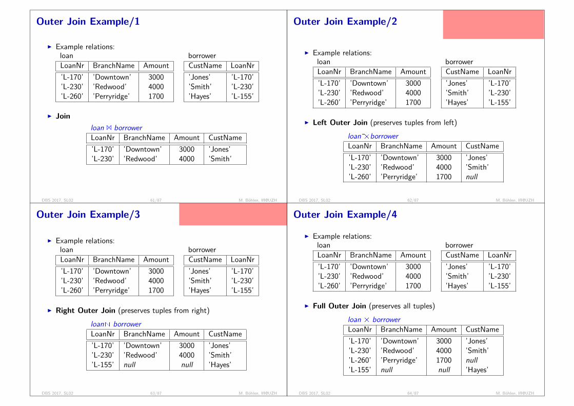
I Example relations:loanLoanNr BranchName Amount’L-170’ ’Downtown’ 3000’L-230’ ’Redwood’ 4000’L-260’ ’Perryridge’ 1700
borrowerCustName LoanNr’Jones’ ’L-170’’Smith’ ’L-230’’Hayes’ ’L-155’
I Joinloan 1 borrowerLoanNr BranchName Amount CustName’L-170’ ’Downtown’ 3000 ’Jones’’L-230’ ’Redwood’ 4000 ’Smith’
DBS 2017, SL02 61/87 M. Böhlen, IfI@UZH
Outer Join Example/2
without outer join? handle two cases:credits with borrowercredits without borrowerrequires NULL as a special constant
I Example relations:loanLoanNr BranchName Amount’L-170’ ’Downtown’ 3000’L-230’ ’Redwood’ 4000’L-260’ ’Perryridge’ 1700
borrowerCustName LoanNr’Jones’ ’L-170’’Smith’ ’L-230’’Hayes’ ’L-155’
I Left Outer Join (preserves tuples from left)loan d|><| borrowerLoanNr BranchName Amount CustName’L-170’ ’Downtown’ 3000 ’Jones’’L-230’ ’Redwood’ 4000 ’Smith’’L-260’ ’Perryridge’ 1700 null
DBS 2017, SL02 62/87 M. Böhlen, IfI@UZH
Outer Join Example/3
in contrast to an inner join, outer joinsare not commutative. implication: muchless possibilities for optimization.
I Example relations:loanLoanNr BranchName Amount’L-170’ ’Downtown’ 3000’L-230’ ’Redwood’ 4000’L-260’ ’Perryridge’ 1700
borrowerCustName LoanNr’Jones’ ’L-170’’Smith’ ’L-230’’Hayes’ ’L-155’
I Right Outer Join (preserves tuples from right)loan |><|d borrowerLoanNr BranchName Amount CustName’L-170’ ’Downtown’ 3000 ’Jones’’L-230’ ’Redwood’ 4000 ’Smith’’L-155’ null null ’Hayes’
DBS 2017, SL02 63/87 M. Böhlen, IfI@UZH
Outer Join Example/4
I Example relations:loanLoanNr BranchName Amount’L-170’ ’Downtown’ 3000’L-230’ ’Redwood’ 4000’L-260’ ’Perryridge’ 1700
borrowerCustName LoanNr’Jones’ ’L-170’’Smith’ ’L-230’’Hayes’ ’L-155’
I Full Outer Join (preserves all tuples)loan d|><|d borrowerLoanNr BranchName Amount CustName’L-170’ ’Downtown’ 3000 ’Jones’’L-230’ ’Redwood’ 4000 ’Smith’’L-260’ ’Perryridge’ 1700 null’L-155’ null null ’Hayes’
DBS 2017, SL02 64/87 M. Böhlen, IfI@UZH
Modification of the Database
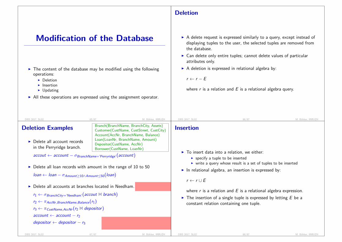
I The content of the database may be modified using the followingoperations:
I DeletionI InsertionI Updating
I All these operations are expressed using the assignment operator.
DBS 2017, SL02 65/87 M. Böhlen, IfI@UZH
Deletion
I A delete request is expressed similarly to a query, except instead ofdisplaying tuples to the user, the selected tuples are removed fromthe database.
I Can delete only entire tuples; cannot delete values of particularattributes only.
I A deletion is expressed in relational algebra by:
r ← r − E
where r is a relation and E is a relational algebra query.
DBS 2017, SL02 66/87 M. Böhlen, IfI@UZH
Deletion Examples Branch(BranchName, BranchCity, Assets)Customer(CustName, CustStreet, CustCity)Account(AccNr, BranchName, Balance)Loan(LoanNr, BranchName, Amount)Depositor(CustName, AccNr)Borrower(CustName, LoanNr)
I Delete all account recordsin the Perryridge branch.accout ← account − σBranchName=’Perryridge’(account)
I Delete all loan records with amount in the range of 10 to 50loan← loan − σAmount≥10∧Amount≤50(loan)
I Delete all accounts at branches located in Needham.
delete accounts; deleteowner of accounts
r1 ← σBranchCity=’Needham’(accout 1 branch)r2 ← πAccNr ,BranchName,Balance(r1)r3 ← πCustName,AccNr (r2 1 depositor)account ← account − r2depositor ← depositor − r3
r1: information about Needham accountsr2: Needham accounts that shall be deletedr3: owner of Needham accounts
DBS 2017, SL02 67/87 M. Böhlen, IfI@UZH
Insertion
I To insert data into a relation, we either:I specify a tuple to be insertedI write a query whose result is a set of tuples to be inserted
I In relational algebra, an insertion is expressed by:
r ← r ∪ E
where r is a relation and E is a relational algebra expression.I The insertion of a single tuple is expressed by letting E be a
constant relation containing one tuple.
DBS 2017, SL02 68/87 M. Böhlen, IfI@UZH

Insertion Examples Branch(BranchName, BranchCity, Assets)Customer(CustName, CustStreet, CustCity)Account(AccNr, BranchName, Balance)Loan(LoanNr, BranchName, Amount)Depositor(CustName, AccNr)Borrower(CustName, LoanNr)
r1: Perryridge Kreditnehmer; account: new account; de-positor: new account owner (no duplicates in RA)
I Insert information into thedatabase specifying thatSmith has $1200 in accountA-973 at the Perryridge branch.account ← account ∪ {(‘A-973‘, ‘Perryridge‘, 1200)}depositor ← depositor ∪ {(‘Smith‘, ‘A-973‘)}
I Provide as a gift for all loan customers in the Perryridge branch, a$200 savings account. Let the loan number serve as the accountnumber for the new savings account.r1 ← σBranchName=’Perryridge’(borrower 1 loan)account ← account ∪ πLoanNr ,BranchName,200(r1)depositor ← depositor ∪ πCustName,LoanNr (r1)
DBS 2017, SL02 69/87 M. Böhlen, IfI@UZH
Updating
I A mechanism to change a value in a tuple without changing allvalues in the tuple; logically this can be expressed by an insertionand deletion; in actual systems updating is much faster thaninserting and deleting.
I In relational algebra this can be expressed by replacing r by theresult computed by the relational algebra expression E ; often theexpression is the generalized projection.
r ← Er ← πF1,F2....,Fi ,...(r)
I Each Fi is eitherI the ith attribute of r , if the ith attribute is not updated, or,I if the attribute is to be updated Fi is an expression, which defines the
new value for the attribute
DBS 2017, SL02 70/87 M. Böhlen, IfI@UZH
Update Examples
I Make interest payments by increasing all balances by 5%.
account ← πAccNr ,BranchName,Balance∗1.05(account)
I Pay all accounts with balances over $10,000 6% interest and pay allothers 5%.
account ←πAccNr ,BranchName,Balance∗1.06(σBalance>100000(account))∪πAccNr ,BranchName,Balance∗1.05(σBalance≤100000(account))
DBS 2017, SL02 71/87 M. Böhlen, IfI@UZH
Relational Calculus
I First Order Predicate LogicI Domain Relational Calculus
venn diagram with significantoverlap of RA, DRC, SQL
DBS 2017, SL02 72/87 M. Böhlen, IfI@UZH
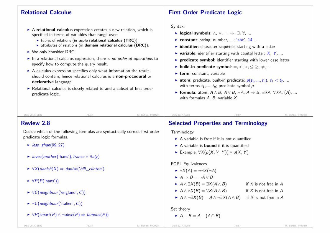
Relational Calculus
I A relational calculus expression creates a new relation, which isspecified in terms of variables that range over:
I tuples of relations (in tuple relational calculus (TRC))I attributes of relations (in domain relational calculus (DRC)).
I We only consider DRC.I In a relational calculus expression, there is no order of operations to
specify how to compute the query result.I A calculus expression specifies only what information the result
should contain; hence relational calculus is a non-procedural ordeclarative language.
I Relational calculus is closely related to and a subset of first orderpredicate logic.
DBS 2017, SL02 73/87 M. Böhlen, IfI@UZH
First Order Predicate Logic
Syntax:I logical symbols: ∧, ∨, ¬, ⇒, ∃, ∀, ...I constant: string, number, ...; ’abc’, 14, ...I identifier: character sequence starting with a letterI variable: identifier starting with capital letter; X , Y , ...I predicate symbol: identifier starting with lower case letterI build-in predicate symbol: =, <,>,≤,≥, 6=, ...I term: constant, variableI atom: predicate, built-in predicate; p(t1, ..., tn), t1 < t2, ...
with terms t1, ..., tn; predicate symbol pI formula: atom, A ∧ B, A ∨ B, ¬A, A⇒ B, ∃XA, ∀XA, (A), ...
with formulas A, B; variable X
DBS 2017, SL02 74/87 M. Böhlen, IfI@UZH
Review 2.8Decide which of the following formulas are syntactically correct first orderpredicate logic formulas.
I less_than(99, 27)
ok
I loves(mother(’hans’), france ∨ italy)
fct and disj are not terms
I ∀X (danish(X )⇒ danish(′bill_clinton′)
missing ) at very end
I ∀P(P(’hans’))
P is not a predicate symbol
I ∀C(neighbour(’england’,C))
ok
I ∃C(neighbour(’italien’,C))
ok
I ∀P(smart(P) ∧ ¬alive(P)⇒ famous(P))
ok
DBS 2017, SL02 75/87 M. Böhlen, IfI@UZH
Selected Properties and TerminologyTerminology
I A variable is free if it is not quantifiedI A variable is bound if it is quantifiedI Example: ∀X (p(X ,Y ,Y )) ∧ q(X ,Y )
FOPL EquivalencesI ∀X (A) = ¬∃X (¬A)I A⇒ B = ¬A ∨ BI A ∧ ∃X (B) = ∃X (A ∧ B) if X is not free in AI A ∧ ∀X (B) = ∀X (A ∧ B) if X is not free in AI A ∧ ¬∃X (B) = A ∧ ¬∃X (A ∧ B) if X is not free in A
Set theoryI A− B = A− (A ∩ B)
DBS 2017, SL02 76/87 M. Böhlen, IfI@UZH

Domain Independence
I Relational calculus only permits expressions that are domainindependent, i.e., expressions that permit sensible answers (e.g., noinfinite results).
I Domain independence is not decidable. There exist various syntacticcriteria that ensure domain independence, e.g., safe expressions,range restricted expressions, etc.
I Examples:I emp(X ) is domain independentI ¬emp(X ) is not domain independentI stud(X ) ∧ ¬emp(X ) is domain independentI X > 6 is not domain independent
DBS 2017, SL02 77/87 M. Böhlen, IfI@UZH
Review 2.9/1Use first order predicate calculus expressions to express the followingnatural language statements:
I Anyone who is dedicated can learn databases.
∀X (dedicated(X )⇒ canlearn(X , ’db’))
I No man is independent.
¬∃X (man(X ) ∧ independent(X ))
I Dogs that bark do not bite.
(dog(X ) ∧ bark(X )⇒ ¬bite(X ))dogd1d2d3
barkd1d2
bited1d3
DBS 2017, SL02 78/87 M. Böhlen, IfI@UZH
Review 2.9/2I Not all men can walk.
¬∀X (man(X )⇒ walk(X ))
I Every person owns a computer.
∀X (person(X )⇒ ∃Y (computer(Y ) ∧ owns(X ,Y )))
I Lars likes everyone who does not like himself.
∀X (¬likes(X ,X )⇒ likes(′lars ′,X ))
DBS 2017, SL02 79/87 M. Böhlen, IfI@UZH
Domain Relational Calculus/1
DRC is relationally complete
Syntax:I logical symbols: ∧, ∨, ¬, ⇒, ∃, ∀, ...I constant: string, number, ...; ’abc’, 14, ...I identifier: character sequence starting with a letterI variable: identifier starting with capital letter; X , Y , ...I predicate symbol: identifier starting with lower case letterI build-in predicate symbol: =, <,>,≤,≥, 6=, ...I term: constant, variableI atom: predicate, built-in predicate; p(X , ..., 22), X < 5000, ...I formula: atom, A ∧ B, A ∨ B, ¬A, A⇒ B, ∃X (A), ∀X (A), (A), ...
I A domain relational calculus query is of the form{ X1, ...,Xn | formula }
DBS 2017, SL02 80/87 M. Böhlen, IfI@UZH
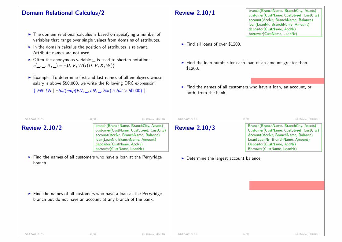
Domain Relational Calculus/2
I The domain relational calculus is based on specifying a number ofvariables that range over single values from domains of attributes.
I In the domain calculus the position of attributes is relevant.Attribute names are not used.
I Often the anonymous variable _ is used to shorten notation:r(_,_,X ,_) = ∃U,V ,W (r(U,V ,X ,W ))
I Example: To determine first and last names of all employees whosesalary is above $50,000, we write the following DRC expression:{ FN, LN | ∃Sal(emp(FN,_, LN,_, Sal) ∧ Sal > 50000) }
DBS 2017, SL02 81/87 M. Böhlen, IfI@UZH
Review 2.10/1 branch(BranchName, BranchCity, Assets)customer(CustName, CustStreet, CustCity)account(AccNr, BranchName, Balance)loan(LoanNr, BranchName, Amount)depositor(CustName, AccNr)borrower(CustName, LoanNr)
final existential quantification is often omitted
I Find all loans of over $1200.
{L,B,A | loan(L,B,A) ∧ A > 1200}
I Find the loan number for each loan of an amount greater than$1200.
{L | ∃A(loan(L,_,A) ∧ A > 1200)}
I Find the names of all customers who have a loan, an account, orboth, from the bank.
{N | loan(N,_) ∨ borrower(N,_)}
DBS 2017, SL02 82/87 M. Böhlen, IfI@UZH
Review 2.10/2 branch(BranchName, BranchCity, Assets)customer(CustName, CustStreet, CustCity)account(AccNr, BranchName, Balance)loan(LoanNr, BranchName, Amount)depositor(CustName, AccNr)borrower(CustName, LoanNr)
I Find the names of all customers who have a loan at the Perryridgebranch.
{N | ∃L(borrower(N, L) ∧ loan(L,′ Perryridge′,_))}
I Find the names of all customers who have a loan at the Perryridgebranch but do not have an account at any branch of the bank.
{N | ∃L(borrower(N, L) ∧ loan(L,′ Perryridge′,_)) ∧¬depositor(N,_)}
DBS 2017, SL02 83/87 M. Böhlen, IfI@UZH
Review 2.10/3 Branch(BranchName, BranchCity, Assets)Customer(CustName, CustStreet, CustCity)Account(AccNr, BranchName, Balance)Loan(LoanNr, BranchName, Amount)Depositor(CustName, AccNr)Borrower(CustName, LoanNr)
I Determine the largest account balance.
{A | account(_,_,A) ∧ ∀B(account(_,_,B)⇒ B ≤ A)}
what happens if ≤ is replaced by <? empty re-sult.
DBS 2017, SL02 84/87 M. Böhlen, IfI@UZH
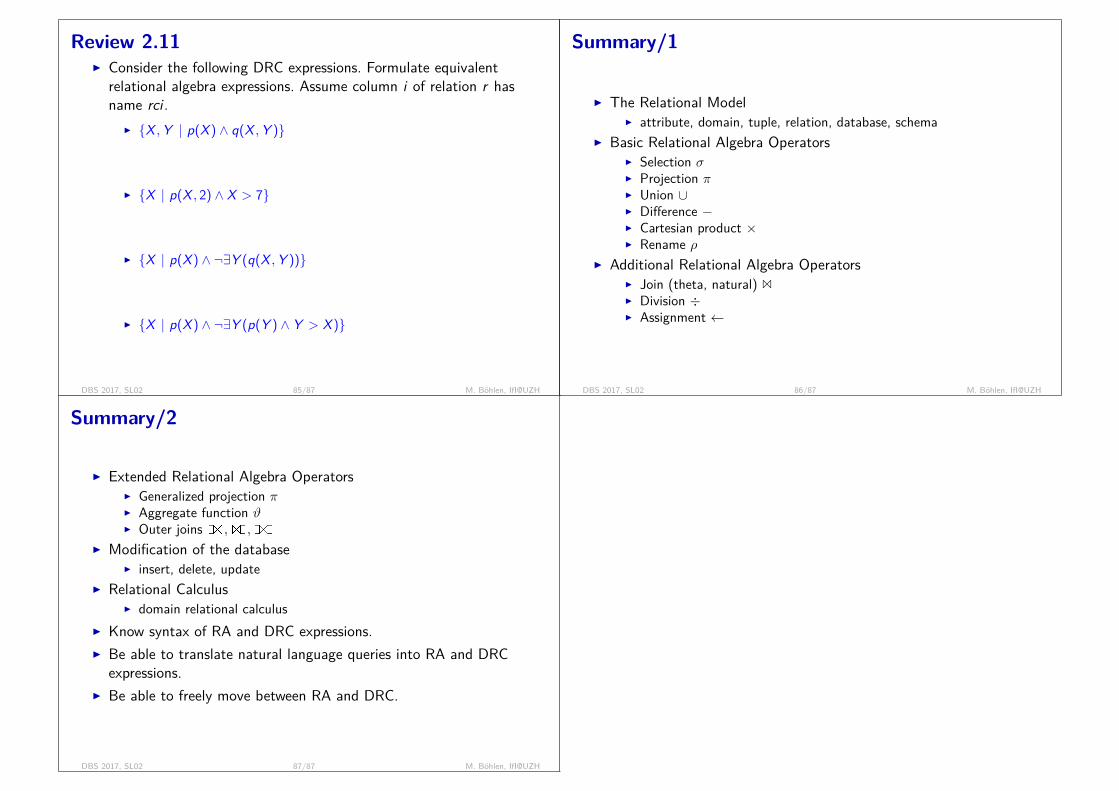
Review 2.11I Consider the following DRC expressions. Formulate equivalent
relational algebra expressions. Assume column i of relation r hasname rci .
I {X ,Y | p(X ) ∧ q(X ,Y )}
πqc1,qc2(σpc1=qc1(p × q))
I {X | p(X , 2) ∧ X > 7}
πpc1(σpc2=2∧pc1>7(p))
I {X | p(X ) ∧ ¬∃Y (q(X ,Y ))}
p − πqc1(q)
I {X | p(X ) ∧ ¬∃Y (p(Y ) ∧ Y > X )}
p−πpc1(σqc1=pc1(p× ρq(qc1)(p)))
DBS 2017, SL02 85/87 M. Böhlen, IfI@UZH
Summary/1
I The Relational ModelI attribute, domain, tuple, relation, database, schema
I Basic Relational Algebra OperatorsI Selection σI Projection πI Union ∪I Difference −I Cartesian product ×I Rename ρ
I Additional Relational Algebra OperatorsI Join (theta, natural) 1I Division ÷I Assignment ←
DBS 2017, SL02 86/87 M. Böhlen, IfI@UZH
Summary/2
I Extended Relational Algebra OperatorsI Generalized projection πI Aggregate function ϑI Outer joins d|><| , |><|d , d|><|d
I Modification of the databaseI insert, delete, update
I Relational CalculusI domain relational calculus
I Know syntax of RA and DRC expressions.I Be able to translate natural language queries into RA and DRC
expressions.I Be able to freely move between RA and DRC.
DBS 2017, SL02 87/87 M. Böhlen, IfI@UZH

Database SystemsSpring 2017
SQLSL03
I Data Definition LanguageI Expressions and PredicatesI Table Expressions, Query Specifications, Query ExpressionsI Subqueries, Duplicates, Null ValuesI Modification of the Database
Reviews: 6 23 39 44 45 50 52 53 54 61 65 68 74 77 83 94
user friendly packaging of RA+requirements from real world applications
goal: concepts + application on concrete ex-amples; abstract from details of syntax
DBS 2017, SL03 1/97 M. Böhlen, IfI@UZH
Literature and Acknowledgments
Reading List for SL03:I Database Systems, Chapters 4 and 5 (sections 5.1 and 5.4), Sixth
Edition, Ramez Elmasri and Shamkant B. Navathe, PearsonEducation, 2010.
These slides were developed by:I Michael Böhlen, University of Zürich, SwitzerlandI Johann Gamper, Free University of Bozen-Bolzano, Italy
The slides are based on the following text books and associated material:I Fundamentals of Database Systems, Fourth Edition, Ramez Elmasri
and Shamkant B. Navathe, Pearson Addison Wesley, 2004.I A. Silberschatz, H. Korth, and S. Sudarshan: Database System
Concepts, McGraw Hill, 2006.
DBS 2017, SL03 2/97 M. Böhlen, IfI@UZH
History/1
I IBM Sequel language developed as part of System R project at theIBM San Jose Research Laboratory
I Renamed Structured Query Language (SQL)I ANSI and ISO standard SQL:
I SQL-86I SQL-89I SQL-92 (also called SQL2)
I entry level: roughly corresponds to SQL-89I intermediate level: half of the new features of SQL-92I full level
I SQL:2003 (also called SQL3)I Commercial systems offer most, if not all, SQL-92 features, plus
varying feature sets from later standards and special proprietaryfeatures.
I Not all examples here may (will!) work on your particular system.
DBS 2017, SL03 3/97 M. Böhlen, IfI@UZH
History/2
I Don Chamberlin holds a Ph.D. fromStanford University.
I He worked at Almaden Research Centerdoing research on database languages andsystems.
I He was a member of the System R researchteam that developed much of today’srelational database technology
I He designed the original SQL database language.I In 2005 Don Chamberlin received an honory doctoral degree from
the University of Zürich for his work on SQL.
http://www.almaden.ibm.com/cs/people/chamberlin/
DBS 2017, SL03 4/97 M. Böhlen, IfI@UZH
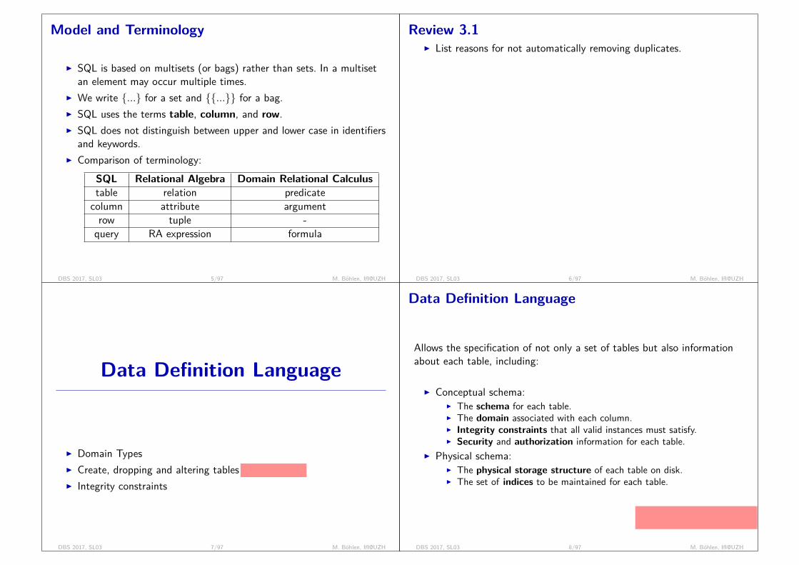
Model and Terminology
I SQL is based on multisets (or bags) rather than sets. In a multisetan element may occur multiple times.
I We write {...} for a set and {{...}} for a bag.I SQL uses the terms table, column, and row.I SQL does not distinguish between upper and lower case in identifiers
and keywords.I Comparison of terminology:
SQL Relational Algebra Domain Relational Calculustable relation predicatecolumn attribute argumentrow tuple -query RA expression formula
DBS 2017, SL03 5/97 M. Böhlen, IfI@UZH
Review 3.1I List reasons for not automatically removing duplicates.
I performance: too expensive to remove; requires sortingI duplicates can be important for applicationI for aggregation duplicates are important
DBS 2017, SL03 6/97 M. Böhlen, IfI@UZH
Data Definition Language
I Domain TypesI Create, dropping and altering tables
schema changes
I Integrity constraints
DBS 2017, SL03 7/97 M. Böhlen, IfI@UZH
Data Definition Language
Allows the specification of not only a set of tables but also informationabout each table, including:
security: e.g., add redundancy torecover lost/corrupted data
I Conceptual schema:I The schema for each table.I The domain associated with each column.I Integrity constraints that all valid instances must satisfy.I Security and authorization information for each table.
I Physical schema:I The physical storage structure of each table on disk.I The set of indices to be maintained for each table.
DBS 2017, SL03 8/97 M. Böhlen, IfI@UZH

Domain Types in SQL
I CHAR(n) Fixed length character string, with user-defined length n.I VARCHAR(n) Variable length character strings, with user-specified
maximum length n.I INTEGER Integer (a finite subset of the integers that is
machine-dependent).I SMALLINT Small integer (a machine-dependent subset of the
integer domain type).I NUMERIC(p,d) Fixed point number, with user-specified precision
of p digits, with n digits to the right of decimal point.I REAL, DOUBLE PRECISION Floating point and double-precision
floating point numbers, with machine-dependent precision.I FLOAT(n) Floating point number, with user-specified precision of
at least n digits.
DBS 2017, SL03 9/97 M. Böhlen, IfI@UZH
Create Table Construct
many additional options, e.g., machine, disk,fill factor of blocks, partitioning, large attri-butes (movies, pictures, XML), caching, log-ging, ordering, chunk size, compression, ...
I An SQL table is defined using the create table command:create table r(
A1D1,A2D2, . . . ,AnDn,(integrity-constraint1),. . . ,(integrity-constraintk))
I r is the name of the tableI each Ai is an column name in the schema of tableI Di is the data type of values in the domain of column Ai
I Example:CREATE TABLE branch (BranchName CHAR(15) NOT NULL,BranchCity CHAR(30),Assets INTEGER )
DBS 2017, SL03 10/97 M. Böhlen, IfI@UZH
Integrity Constraints in Create Table/1
I not nullI primary key (A1, . . . ,An)I foreign key (A1, . . . ,An) references T (B1, . . . ,Bn)
Example: Declare BranchName as the primary key for branchCREATE TABLE branch (BranchName CHAR(15),BranchCity CHAR(30),Assets INTEGER,PRIMARY KEY (BranchName) )
In SQL a primary key declaration on a column automatically ensuresnot null.
DBS 2017, SL03 11/97 M. Böhlen, IfI@UZH
Integrity Constraints in Create Table/2
important for data quality; forces people to enter complete data; data quality mustbe ensured when data is entered; later fixes are very expensive or impossible.
Unternehmen mit DB ohne Fremdschlüssel! possible reasons?there are always exceptions; no address; secret account nr, etc;shall this be allowed/supported?no!; only decision you can make is where do you want to deal with the problem; solve it whencollecting and storing the data or solve it when querying the data; many examples in real worldwhere missing data is not permitted (Kreisbüro, UZH, ...)
Example: Define AccNr as foreign key in table depositor :CREATE TABLE depositor (CustName VARCHAR(15),AccNr INTEGER,FOREIGN KEY (AccNr) REFERENCES account(AccNr))
DBS 2017, SL03 12/97 M. Böhlen, IfI@UZH

Notation/1
I SQL is a comprehensive language and offers multiple syntacticconstructs to define table and integrity constraints.
I The exact syntax depends on the database system and even theversion.
I We use a small core of SQL that is general and is mostlyindependent of the database system and the version.
I Selected peculiarities of the syntax, especially when relevant for theexercises, will be pointed out.
I In case of syntax problems look up the exact syntax (manual, web,forum, etc).
DBS 2017, SL03 13/97 M. Böhlen, IfI@UZH
Notation/2
I In SQL small and capital letters are irrelevant (e.g., SELECT, select,seLEct).
I In some systems the capitalization of identifiers is relevant (e.g.,table names in MySQL on Linux).
I Small and capital letters are relevant if identifiers are put in quotes(’CustName’).
I In Oracle and PostgreSQL single quotes must be used (’abcde’).I In MySQL single (’abcde’) and double (“abcde”) quotes are
permitted.
DBS 2017, SL03 14/97 M. Böhlen, IfI@UZH
Notation/3
I On the course slides we use bold face for reserved words (e.g.,select).
I On the slides code examples are typeset in blue. Keywords arecapitalized and bold face.
I In program code reserved words are usually capitalized (e.g.,SELECT).
I The end of an SQL statement is often marked by a semicolon:SELECT * FROM account;
DBS 2017, SL03 15/97 M. Böhlen, IfI@UZH
Drop and Alter Table Constructs
I The drop table command deletes all information about the droppedtable from the database.
I The alter table command is used to add columns to an existingtable:alter table r add A D
where A is the name of the column to be added to table r and D isthe domain of A.
I All tuples in the table are assigned null as the value for the newcolumn.
I The alter table command can also be used to drop columns of atable:alter table r drop A
where A is the name of a column of table r
DBS 2017, SL03 16/97 M. Böhlen, IfI@UZH
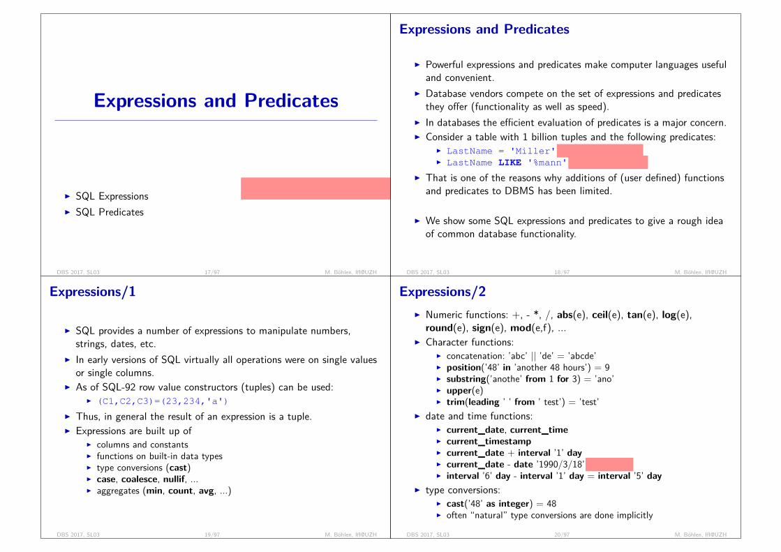
Expressions and Predicates
maximizing expressiveness while ensuringperformance
I SQL ExpressionsI SQL Predicates
DBS 2017, SL03 17/97 M. Böhlen, IfI@UZH
Expressions and Predicates
I Powerful expressions and predicates make computer languages usefuland convenient.
I Database vendors compete on the set of expressions and predicatesthey offer (functionality as well as speed).
I In databases the efficient evaluation of predicates is a major concern.I Consider a table with 1 billion tuples and the following predicates:
I LastName = 'Miller'
simple; eg phone book
I LastName LIKE '%mann'
good plan is difficult
I That is one of the reasons why additions of (user defined) functionsand predicates to DBMS has been limited.
I We show some SQL expressions and predicates to give a rough ideaof common database functionality.
DBS 2017, SL03 18/97 M. Böhlen, IfI@UZH
Expressions/1
I SQL provides a number of expressions to manipulate numbers,strings, dates, etc.
I In early versions of SQL virtually all operations were on single valuesor single columns.
I As of SQL-92 row value constructors (tuples) can be used:I (C1,C2,C3)=(23,234,'a')
I Thus, in general the result of an expression is a tuple.I Expressions are built up of
I columns and constantsI functions on built-in data typesI type conversions (cast)I case, coalesce, nullif, ...I aggregates (min, count, avg, ...)
DBS 2017, SL03 19/97 M. Böhlen, IfI@UZH
Expressions/2I Numeric functions: +, - *, /, abs(e), ceil(e), tan(e), log(e),round(e), sign(e), mod(e,f), ...
I Character functions:I concatenation: ’abc’ || ’de’ = ’abcde’I position(’48’ in ’another 48 hours’) = 9I substring(’anothe’ from 1 for 3) = ’ano’I upper(e)I trim(leading ’ ’ from ’ test’) = ’test’
I date and time functions:I current_date, current_timeI current_timestampI current_date + interval ’1’ dayI current_date - date ’1990/3/18’
age in days
I interval ’6’ day - interval ’1’ day = interval ’5’ dayI type conversions:
I cast(’48’ as integer) = 48I often “natural” type conversions are done implicitly
DBS 2017, SL03 20/97 M. Böhlen, IfI@UZH

Expressions/3
I conditional statement:casewhen cond1 then result1...when condN then resultNelse resultXend
I coalesce(val1, ..., valN)returns the first value that is not null (and null if all values are equalto null)
I nullif(e1,e2)returns null if e1 and e2 are identical; useful if missing information isnot represented with null; nullif(cost, 9999)
DBS 2017, SL03 21/97 M. Böhlen, IfI@UZH
Predicates
step from binary logic to 3-valued logic is a non-trivial
I Predicates evaluate to true, false or unknownI boolean connectives: and, or, notI =, <>,<,>,<=, >=I e [not] between e1 and e2I e is [not] nullI e in (e1, ..., eN)I e1 like e2
example: Name like ’_ross%’wildcards: % 0-n characters, _ 1 character
DBS 2017, SL03 22/97 M. Böhlen, IfI@UZH
Review 3.2I Rewrite
1. (X,Y,Z)=(1,2,3)2. (X,Y,Z)<(1,2,3)
to equivalent expressions without row value constructors.
1. X=1 AND Y=2 AND Z=32. (X<1) OR (X=1 AND Y<2) OR (X=1 AND Y=2 AND Z<3)
I Identify the problem with the predicateX>0 AND 1/X>0.1
and propose a solution.
- AND is not evaluated left to right and stopped asap- AND corresponds to & in Java, not &&- division by zero is possible- CASE WHEN x>0 THEN 1/x>0.1 ELSE FALSE END
DBS 2017, SL03 23/97 M. Böhlen, IfI@UZH
Query Expressions
I Table expressionsI Query specificationsI Query Expressions
DBS 2017, SL03 24/97 M. Böhlen, IfI@UZH

Structure of SQL Queries/1
I The main building block of SQL are “queries” (will be defined moreprecisely below).
I SQL is used very heavily in the real world.I SQL is much more than a simple select-from-where, such as
SELECT *FROM loanWHERE LName = 'Bohr'
I Many peopleI Underestimate SQLI Do not properly understand the concepts of SQLI Do not understand how to work with a declarative language and sets
(this requires some practice and getting used to)
DBS 2017, SL03 25/97 M. Böhlen, IfI@UZH
Structure of SQL Queries/2I A typical SQL query has the form:
select clausefrom clausewhere clausegroup clausehaving clause
tableexpression
queryspecification
union
select clausefrom clausewhere clausegroup clausehaving clause
tableexpression
queryspecification
queryexpression
I The result of an SQL query is a (virtual) table.DBS 2017, SL03 26/97 M. Böhlen, IfI@UZH
Evaluation of Query SpecificationsConceptually, an SQL query specification is processed as follows.
selectfromwheregroup
having
list of tablestable
subset of table(some tuplesare dropped)
multiple tables(grouped table)
subset of groups(some groups aredropped)
returns one row per group; possiblycompute aggregate for each group
DBS 2017, SL03 27/97 M. Böhlen, IfI@UZH
Evaluation of SQL Queries
1. Form the cross product of the tables in the from clause
× in RA
2. Eliminate tuples that do not satisfy the where clause
σ in RA
3. Group the remaining tuples according to the group clause
4. Eliminate groups that do not satisfy the having clause
5. Evaluate the expressions in the select clause
π in RA
6. One result tuple is returned for each group
7. Eliminate duplicates if distinct is specified
8. Compute query specifications independently and apply setoperations (union, excpet, intersect)
9. Sort all result tuples according to order clause
DBS 2017, SL03 28/97 M. Böhlen, IfI@UZH
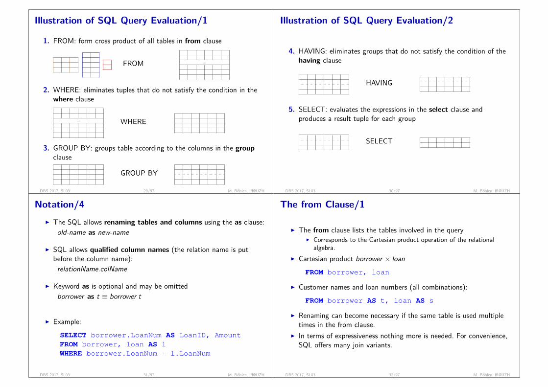
Illustration of SQL Query Evaluation/1
1. FROM: form cross product of all tables in from clause
FROM ...
2. WHERE: eliminates tuples that do not satisfy the condition in thewhere clause
... WHERE
3. GROUP BY: groups table according to the columns in the groupclause
GROUP BY
DBS 2017, SL03 29/97 M. Böhlen, IfI@UZH
Illustration of SQL Query Evaluation/2
4. HAVING: eliminates groups that do not satisfy the condition of thehaving clause
HAVING
5. SELECT: evaluates the expressions in the select clause andproduces a result tuple for each group
SELECT
DBS 2017, SL03 30/97 M. Böhlen, IfI@UZH
Notation/4I The SQL allows renaming tables and columns using the as clause:
old-name as new-name
I SQL allows qualified column names (the relation name is putbefore the column name):relationName.colName
I Keyword as is optional and may be omittedborrower as t ≡ borrower t
I Example:SELECT borrower.LoanNum AS LoanID, AmountFROM borrower, loan AS lWHERE borrower.LoanNum = l.LoanNum
DBS 2017, SL03 31/97 M. Böhlen, IfI@UZH
The from Clause/1
I The from clause lists the tables involved in the queryI Corresponds to the Cartesian product operation of the relational
algebra.I Cartesian product borrower × loan
FROM borrower, loan
I Customer names and loan numbers (all combinations):FROM borrower AS t, loan AS s
I Renaming can become necessary if the same table is used multipletimes in the from clause.
I In terms of expressiveness nothing more is needed. For convenience,SQL offers many join variants.
DBS 2017, SL03 32/97 M. Böhlen, IfI@UZH

The from Clause/2
I SQL supports many different join:I FROM t1 CROSS JOIN t2
I Cartesian product
I FROM t1 JOIN t2 ON t1.a < t2.b
I Theta join
I FROM t1 LEFT OUTER JOIN t2 ON t1.a = t2.b
I left outer join
I FROM t1 NATURAL INNER JOIN t2
I Natural join
I FROM t1 NATURAL INNER JOIN t2 USING (name)
I Limited natural join (not all pair-wise equal columns are used for thenatural join; only the ones specified in the using clause)
DBS 2017, SL03 33/97 M. Böhlen, IfI@UZH
The from Clause/3
I Table loanLoanNum BranchName Amount’L-170’ ’Downtown’ 3000’L-230’ ’Redwood’ 4000’L-260’ ’Perryridge’ 1700
I Table borrowerCustName LoanNum’Jones’ ’L-170’’Smith’ ’L-230’’Hayes’ ’L-155’
I Note: borrower information missing for L-260 and loan informationmissing for L-155
DBS 2017, SL03 34/97 M. Böhlen, IfI@UZH
The from Clause/4
main advantage: semantics is easier to understand
I FROM loan INNER JOIN borrower ONloan.LoanNum = borrower.LoanNum
LoanNum BranchName Amount CustName LoanNum’L-170’ ’Downtown’ 3000 ’Jones’ ’L-170’’L-230’ ’Redwood’ 4000 ’Smith’ ’L-230’
I FROM loan LEFT OUTER JOIN borrower ONloan.LoanNum = borrower.LoanNum
LoanNum BranchName Amount CustName LoanNum’L-170’ ’Downtown’ 3000 ’Jones’ ’L-170’’L-230’ ’Redwood’ 4000 ’Smith’ ’L-230’’L-260’ ’Perryridge’ 1700 null null
DBS 2017, SL03 35/97 M. Böhlen, IfI@UZH
The from Clause/5
I FROM loan NATURAL INNER JOIN borrower
LoanNum BranchName Amount CustName’L-170’ ’Downtown’ 3000 ’Jones’’L-230’ ’Redwood’ 4000 ’Smith’
I FROM loan NATURAL RIGHT OUTER JOIN borrower
LoanNum BranchName Amount CustName’L-170’ ’Downtown’ 3000 ’Jones’’L-230’ ’Redwood’ 4000 ’Smith’’L-155’ null null ’Hayes’
DBS 2017, SL03 36/97 M. Böhlen, IfI@UZH

The where Clause/1
I The where clause specifies conditions that the result tuples mustsatisfy.
I The where clause takes the virtual table produced by the fromclause and filters out those rows that do not satisfy the condition.
I Example: loan number of loans from the Perryridge branch with loanamounts greater than $1200.FROM loanWHERE BrancheName = 'Perryridge'AND Amount > 1200
LoanNum BranchName Amount’L-260’ ’Perryridge’ 1700
I The where clause corresponds to the selection predicate.
DBS 2017, SL03 37/97 M. Böhlen, IfI@UZH
The where Clause/2
I In SQL predicates can be combined using the logical connectivesand, or, and not.
I The where clause can be used to specify join and selectionconditions.
I SQL includes a between comparison operatorI Example: Find the loan number of those loans with loan amounts
between $90,000 and $100,000 (that is, ≥ $90,000 and ≤$100,000)SELECT LoanNumFROM loanWHERE Amount BETWEEN 90000 AND 100000
DBS 2017, SL03 38/97 M. Böhlen, IfI@UZH
Review 3.3Translate the following RA expressions into equivalent SQL fragments.
1. R × S
FROM r, s
2. (R × S)× T
FROM r, s, t
3. σA>5(R)
FROM rWHERE A > 5
4. σA>5(σB=4(R))
FROM rWHERE A > 5 AND B = 4
5. σA=X (R × S)
FROM r, sWHERE A = X
6. σA>5(R)× σX=7(S)
FROM r, sWHERE A > 5 AND X = 7
DBS 2017, SL03 39/97 M. Böhlen, IfI@UZH
The group Clause/1I The group clause takes the table produced by the where clause and
returns a grouped table.I Example: Accounts grouped by branch.
FROM accountGROUP BY BranchName
accountAccNr BranchName Balance’A-101’ ’Downtown’ 500’A-215’ ’Perryridge’ 700’A-102’ ’Perryridge’ 400’A-305’ ’Perryridge’ 350’A-222’ ’Perryridge’ 700’A-201’ ’Brighton’ 900’A-217’ ’Brighton’ 750
DBS 2017, SL03 40/97 M. Böhlen, IfI@UZH
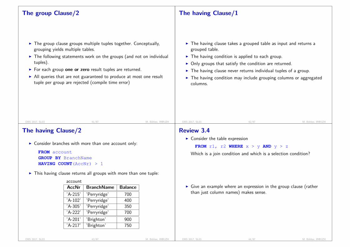
The group Clause/2
I The group clause groups multiple tuples together. Conceptually,grouping yields multiple tables.
I The following statements work on the groups (and not on individualtuples).
I For each group one or zero result tuples are returned.I All queries that are not guaranteed to produce at most one result
tuple per group are rejected (compile time error)
DBS 2017, SL03 41/97 M. Böhlen, IfI@UZH
The having Clause/1
I The having clause takes a grouped table as input and returns agrouped table.
I The having condition is applied to each group.I Only groups that satisfy the condition are returned.I The having clause never returns individual tuples of a group.I The having condition may include grouping columns or aggregated
columns.
DBS 2017, SL03 42/97 M. Böhlen, IfI@UZH
The having Clause/2
I Consider branches with more than one account only:FROM accountGROUP BY BranchNameHAVING COUNT(AccNr) > 1
I This having clause returns all groups with more than one tuple:accountAccNr BranchName Balance’A-215’ ’Perryridge’ 700’A-102’ ’Perryridge’ 400’A-305’ ’Perryridge’ 350’A-222’ ’Perryridge’ 700’A-201’ ’Brighton’ 900’A-217’ ’Brighton’ 750
DBS 2017, SL03 43/97 M. Böhlen, IfI@UZH
Review 3.4I Consider the table expression
FROM r1, r2 WHERE x > y AND y > z
Which is a join condition and which is a selection condition?
depends on schema. assume r1(X,Y) and r2(Z,U). then- X>Y is a selection condition- Y>Z is a join condition
I Give an example where an expression in the group clause (ratherthan just column names) makes sense.
- GROUP BY (salary + bonus) / 1000 (integer division)name salary bonuspam 4200 0tom 3200 700lena 200 3900
DBS 2017, SL03 44/97 M. Böhlen, IfI@UZH
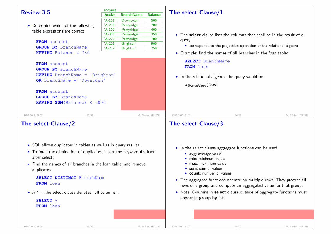
Review 3.5 accountAccNr BranchName Balance’A-101’ ’Downtown’ 500’A-215’ ’Perryridge’ 700’A-102’ ’Perryridge’ 400’A-305’ ’Perryridge’ 350’A-222’ ’Perryridge’ 700’A-201’ ’Brighton’ 900’A-217’ ’Brighton’ 750
I Determine which of the followingtable expressions are correct.
FROM accountGROUP BY BranchNameHAVING Balance < 730
FROM accountGROUP BY BranchNameHAVING BranchName = 'Brighton'OR BranchName = 'Downtown'
FROM accountGROUP BY BranchNameHAVING SUM(Balance) < 1000
stmt1: incorrect. balancenot unique per group.stmt2: ok. returns 2 groupsand 2 result tuples.stmt3: ok.
in a select clause it is pos-sible to have either 1) grou-ped attributes since they areunique for each group or2) aggregated attributes sin-ce this yields one value pergroup
DBS 2017, SL03 45/97 M. Böhlen, IfI@UZH
The select Clause/1
I The select clause lists the columns that shall be in the result of aquery.
I corresponds to the projection operation of the relational algebraI Example: find the names of all branches in the loan table:
SELECT BranchNameFROM loan
I In the relational algebra, the query would be:πBranchName(loan)
DBS 2017, SL03 46/97 M. Böhlen, IfI@UZH
The select Clause/2
distinct is super GAU for DBMS:collect + wait + sort.
I SQL allows duplicates in tables as well as in query results.I To force the elimination of duplicates, insert the keyword distinct
after select.I Find the names of all branches in the loan table, and remove
duplicates:SELECT DISTINCT BranchNameFROM loan
I A * in the select clause denotes “all columns”:SELECT *FROM loan
DBS 2017, SL03 47/97 M. Böhlen, IfI@UZH
The select Clause/3
reason: there may only be one result tuple per group; a group column and aggre-gate ensure that there is only one value.
I In the select clause aggregate functions can be used.I avg: average valueI min: minimum valueI max: maximum valueI sum: sum of valuesI count: number of values
I The aggregate functions operate on multiple rows. They process allrows of a group and compute an aggregated value for that group.
I Note: Columns in select clause outside of aggregate functions mustappear in group by list
DBS 2017, SL03 48/97 M. Böhlen, IfI@UZH
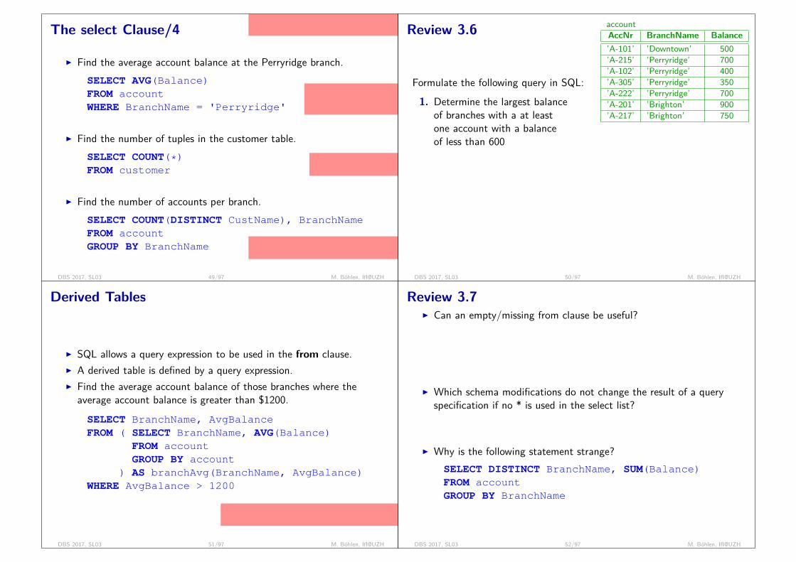
The select Clause/4
duplicates and nulls: initial aggregate va-lue: 0 for count; null for others
I Find the average account balance at the Perryridge branch.SELECT AVG(Balance)FROM accountWHERE BranchName = 'Perryridge'
all aggregates, exceptcount(*), consider du-plicates and ignore nulls
I Find the number of tuples in the customer table.SELECT COUNT(*)FROM customer
count(*) considers du-plicates and nulls
I Find the number of accounts per branch.SELECT COUNT(DISTINCT CustName), BranchNameFROM accountGROUP BY BranchName
count(distinct ...) ignores duplicates andnulls; equivalent for other aggregate fcts
DBS 2017, SL03 49/97 M. Böhlen, IfI@UZH
Review 3.6 accountAccNr BranchName Balance’A-101’ ’Downtown’ 500’A-215’ ’Perryridge’ 700’A-102’ ’Perryridge’ 400’A-305’ ’Perryridge’ 350’A-222’ ’Perryridge’ 700’A-201’ ’Brighton’ 900’A-217’ ’Brighton’ 750
Formulate the following query in SQL:1. Determine the largest balance
of branches with a at leastone account with a balanceof less than 600
SELECT MAX(Balance), FNameFROM accountGROUP BY BranchNameHAVING MIN(Balance) < 600
DBS 2017, SL03 50/97 M. Böhlen, IfI@UZH
Derived Tables
nesting in the from clause is important becauseof orthogonality; makes a language user-friendly.
I SQL allows a query expression to be used in the from clause.I A derived table is defined by a query expression.I Find the average account balance of those branches where the
average account balance is greater than $1200.SELECT BranchName, AvgBalanceFROM ( SELECT BranchName, AVG(Balance)
FROM accountGROUP BY account
) AS branchAvg(BranchName, AvgBalance)WHERE AvgBalance > 1200
DBS 2017, SL03 51/97 M. Böhlen, IfI@UZH
Review 3.7I Can an empty/missing from clause be useful?
- SELECT CURRENT_DATE;- SELECT 7*3;PostgreSQL: missing from clause OK; Oracle select 7*3 from dual;dual is a dummy table with 1 row and 1 column
I Which schema modifications do not change the result of a queryspecification if no * is used in the select list?
adding columns does not change the result (useful in real world)
I Why is the following statement strange?SELECT DISTINCT BranchName, SUM(Balance)FROM accountGROUP BY BranchName
grouping returns 1 row per BranchName; there are no duplicates
DBS 2017, SL03 52/97 M. Böhlen, IfI@UZH

Review 3.8I Consider schema PC(Model,Speed,RAM,Price). Determine
1. the price of the most expensive PC
SELECT MAX(Price) FROM pc ;
2. the price and model of the most expensive PC
SELECT MAX(Price), Model FROM pc ;illegal; Model is not a grouping attribute
SELECT MAX(Price), Model FROM pc GROUP BY Model ;wrong; determines for each model the most expensive PC
SELECT MAX(Price), ModelFROM pc, (SELECT MAX(Price) AS TopPrice FROM pc) AS r;WHERE Price = TopPrice ;
DBS 2017, SL03 53/97 M. Böhlen, IfI@UZH
Review 3.9I Consider schema Emp(Name, Sal, DName). For each
department with more than 3 employees determine the number ofemployees earning more than 40K.
SELECT DName, COUNT(*)FROM empWHERE Sal>40KGROUP BY DNameHAVING COUNT (*)>3
wrong. considers only emps who earn more than 40K. must apply having before where.
SELECT DName, COUNT(*)FROM emp
NATURAL JOIN(SELECT DNameFROM empGROUP BY DNameHAVING COUNT(*)>3) AS r
WHERE Sal>40KGROUP BY DName
DBS 2017, SL03 54/97 M. Böhlen, IfI@UZH
Query Expressions/1
union is expensive (duplicate elimination); union all is very cheap.semantics:- no dupl + union: ok- dupl + union all: ok- dupl + union: ??? (weird)
I The set operations union, intersect, and except operate on tablesand correspond to the relational algebra operations ∪,∩,−.
I Each of the above operations automatically eliminates duplicates; toretain all duplicates use the corresponding multiset versions unionall, intersect all, and except all.
Suppose a tuple occurs m times in r and n times in s, then, itoccurs:
I m + n times in r union all sI min(m, n) times in r intersect all sI max(0,m − n) times in r except all s
DBS 2017, SL03 55/97 M. Böhlen, IfI@UZH
Query Expressions/2
I Find all customers who have a loan, an account, or both:SELECT CustName FROM depositorUNIONSELECT CustName FROM borrower
I Find all customers who have both a loan and an account:SELECT CustName FROM depositorINTERSECTSELECT CustName FROM borrower
I Find all customers who have an account but no loan:SELECT CustName FROM depositorEXCEPTSELECT CustName FROM borrower
DBS 2017, SL03 56/97 M. Böhlen, IfI@UZH
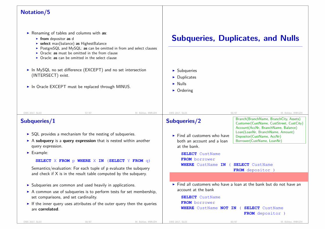
Notation/5
I Renaming of tables and columns with as:I from depositor as dI select max(balance) as HighestBalanceI PostgreSQL and MySQL: as can be omitted in from and select clausesI Oracle: as must be omitted in the from clauseI Oracle: as can be omitted in the select clause
I In MySQL no set difference (EXCEPT) and no set intersection(INTERSECT) exist.
I In Oracle EXCEPT must be replaced through MINUS.
DBS 2017, SL03 57/97 M. Böhlen, IfI@UZH
Subqueries, Duplicates, and Nulls
I SubqueriesI DuplicatesI NullsI Ordering
DBS 2017, SL03 58/97 M. Böhlen, IfI@UZH
Subqueries/1
I SQL provides a mechanism for the nesting of subqueries.I A subquery is a query expression that is nested within another
query expression.I Example:
SELECT X FROM p WHERE X IN (SELECT Y FROM q)
Semantics/evaluation: For each tuple of p evaluate the subqueryand check if X is in the result table computed by the subquery.
I Subqueries are common and used heavily in applications.I A common use of subqueries is to perform tests for set membership,
set comparisons, and set cardinality.I If the inner query uses attributes of the outer query then the queries
are correlated.
DBS 2017, SL03 59/97 M. Böhlen, IfI@UZH
Subqueries/2 Branch(BranchName, BranchCity, Assets)Customer(CustName, CustStreet, CustCity)Account(AccNr, BranchName, Balance)Loan(LoanNr, BranchName, Amount)Depositor(CustName, AccNr)Borrower(CustName, LoanNr)
in predicate: check for each CustNamesubquery: 1) compute once, store as temporary table or 2) compute for each tuple of borrower
I Find all customers who haveboth an account and a loanat the bank.SELECT CustNameFROM borrowerWHERE CustName IN ( SELECT CustName
FROM depositor )
I Find all customers who have a loan at the bank but do not have anaccount at the bankSELECT CustNameFROM borrowerWHERE CustName NOT IN ( SELECT CustName
FROM depositor )
DBS 2017, SL03 60/97 M. Böhlen, IfI@UZH

Review 3.10I Give an SQL query that determines customers who have a loan and
an account such that the account number is larger than the loannumber. Describe the evaluation of the query for relations
I Borrower(CustName,LoanNr); borrower = { (A,18), (B,19), (C,2) }I Depositor(CustName,AccNr); depositor = { (A,17), (B,20), (D,8) }
SELECT CustNameFROM borrowerWHERE CustName IN ( SELECT CustName
FROM depositorWHERE AccNr>LoanNr )
1. for (A,18) the subquery result is {(B)} and in predicate is FALSE2. for (B,19) the subquery result is {(B)} and in predicate is TRUE3. for (C,2) the subquery result is {(A), (B), (D)} and in predicate is FALSE
result = CustNameB
DBS 2017, SL03 61/97 M. Böhlen, IfI@UZH
Subqueries/3 Branch(BranchName, BranchCity, Assets)Customer(CustName, CustStreet, CustCity)Account(AccNr, BranchName, Balance)Loan(LoanNr, BranchName, Amount)Depositor(CustName, AccNr)Borrower(CustName, LoanNr)I Find all customers who have
both an account and a loanat the Perryridge branch
SELECT CustNameFROM borrower, loanWHERE borrower.LoanNum = loan.LoanNumAND BranchName = 'Perryridge'AND (BranchName, CustName) IN (
SELECT BranchName, CustNameFROM depositor, accountWHERE depositor.AccNr = account.AccNr)
SQL permits tuple instead of value.
DBS 2017, SL03 62/97 M. Böhlen, IfI@UZH
Subqueries/4 Branch(BranchName, BranchCity, Assets)Customer(CustName, CustStreet, CustCity)Account(AccNr, BranchName, Balance)Loan(LoanNr, BranchName, Amount)Depositor(CustName, AccNr)Borrower(CustName, LoanNr)
which stmt is easy/difficult?
Comparing sets:I Find all branches that have
greater assets than somebranch located in Brooklyn.SELECT t.BranchNameFROM branch AS t, branch AS sWHERE t.Assets > s.AssetsAND s.BranchCity = 'Brooklyn'
I Same query using > some clauseSELECT BranchNameFROM branchWHERE assets > SOME (SELECT assetsFROM branchWHERE BranchCity = 'Brooklyn' )
DBS 2017, SL03 63/97 M. Böhlen, IfI@UZH
Subqueries/5I F <comp> some r ⇔ ∃t ∈ r such that (F <comp> t)
Where <comp> can be: <,≤ , >,=, 6=
(5 < some056
) = true
(read: 5 < some tuple in the table)
(5 < some 05 ) = false
(5 = some 05 ) = true
≡ (5 IN05 ) = true
(5 6= some 05 ) = true (since 0 6= 5)
6≡ (5 NOT IN05 ) = false
(= some) ≡ inHowever, (6= some) 6≡ not in
DBS 2017, SL03 64/97 M. Böhlen, IfI@UZH
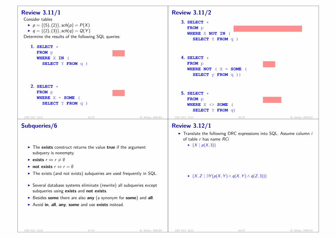
Review 3.11/1Consider tables
I p = {(5), (2)}, sch(p) = P(X )I q = {(2), (3)}, sch(q) = Q(Y )
Determine the results of the following SQL queries:
1. SELECT *FROM pWHERE X IN (SELECT Y FROM q )
{(2)}
2. SELECT *FROM pWHERE X = SOME (SELECT Y FROM q )
{(2)}
DBS 2017, SL03 65/97 M. Böhlen, IfI@UZH
Review 3.11/23. SELECT *
FROM pWHERE X NOT IN (SELECT Y FROM q )
{(5)} ≡ where not (X in (select Y from q))
4. SELECT *FROM pWHERE NOT ( X = SOME (SELECT y FROM q ))
{(5)}
5. SELECT *FROM pWHERE X <> SOME (SELECT Y FROM q)
{(2), (5)}
DBS 2017, SL03 66/97 M. Böhlen, IfI@UZH
Subqueries/6
I The exists construct returns the value true if the argumentsubquery is nonempty.
I exists r ⇔ r 6= ∅I not exists r ⇔ r = ∅I The exists (and not exists) subqueries are used frequently in SQL.
I Several database systems eliminate (rewrite) all subqueries exceptsubqueries using exists and not exists.
I Besides some there are also any (a synonym for some) and all.I Avoid in, all, any, some and use exists instead.
DBS 2017, SL03 67/97 M. Böhlen, IfI@UZH
Review 3.12/1I Translate the following DRC expressions into SQL. Assume column i
of table r has name RCiI {X | p(X , 3)}
SELECT PC1FROM pWHERE PC2 = 3
I {X ,Z | ∃Y (p(X ,Y ) ∧ q(X ,Y ) ∧ q(Z , 3))}
SELECT PC1, q2.QC2FROM p, q q1, q q2WHERE PC1 = q1.QC1AND PC2 = q1.QC2AND q2.QC2 = 3
DBS 2017, SL03 68/97 M. Böhlen, IfI@UZH
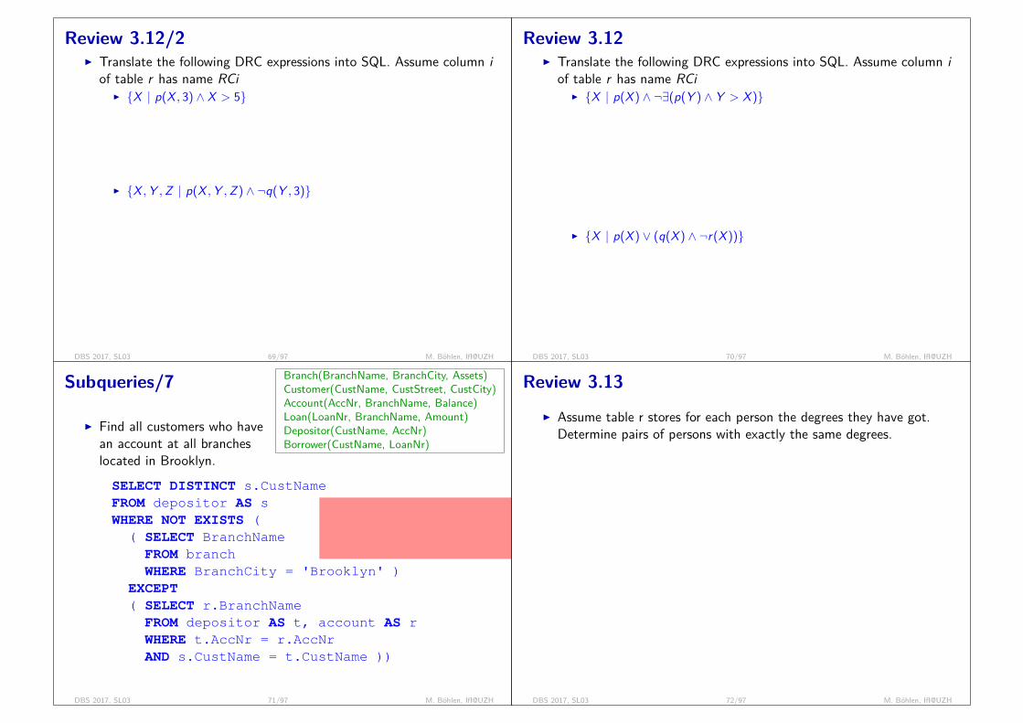
Review 3.12/2I Translate the following DRC expressions into SQL. Assume column i
of table r has name RCiI {X | p(X , 3) ∧ X > 5}
SELECT PC1FROM pWHERE PC1 > 5 AND PC2 = 3
I {X ,Y ,Z | p(X ,Y ,Z ) ∧ ¬q(Y , 3)}
SELECT *FROM pWHERE NOT EXISTS (
SELECT *FROM qWHERE QC1 = PC2AND PC2 = 3 )
DBS 2017, SL03 69/97 M. Böhlen, IfI@UZH
Review 3.12I Translate the following DRC expressions into SQL. Assume column i
of table r has name RCiI {X | p(X ) ∧ ¬∃(p(Y ) ∧ Y > X )}
SELECT PC1FROM pWHERE NOT EXISTS (
SELECT *FROM p p2WHERE p2.PC1 > p.PC1 )
I {X | p(X ) ∨ (q(X ) ∧ ¬r(X ))}
SELECT * FROM pUNION( SELECT * FROM q
EXCEPTSELECT * FROM r
DBS 2017, SL03 70/97 M. Böhlen, IfI@UZH
Subqueries/7 Branch(BranchName, BranchCity, Assets)Customer(CustName, CustStreet, CustCity)Account(AccNr, BranchName, Balance)Loan(LoanNr, BranchName, Amount)Depositor(CustName, AccNr)Borrower(CustName, LoanNr)
- customers (depositors)- such that there does not exist- a branch in Brooklyn- where- this customer does not have an account
I Find all customers who havean account at all brancheslocated in Brooklyn.SELECT DISTINCT s.CustNameFROM depositor AS sWHERE NOT EXISTS (( SELECT BranchNameFROM branchWHERE BranchCity = 'Brooklyn' )
EXCEPT( SELECT r.BranchNameFROM depositor AS t, account AS rWHERE t.AccNr = r.AccNrAND s.CustName = t.CustName ))
DBS 2017, SL03 71/97 M. Böhlen, IfI@UZH
Review 3.13I Assume table r stores for each person the degrees they have got.
Determine pairs of persons with exactly the same degrees.
N DX D1Y D1Y D3Z D1Z D3U D2U D3
N1 N2Y Z
DBS 2017, SL03 72/97 M. Böhlen, IfI@UZH
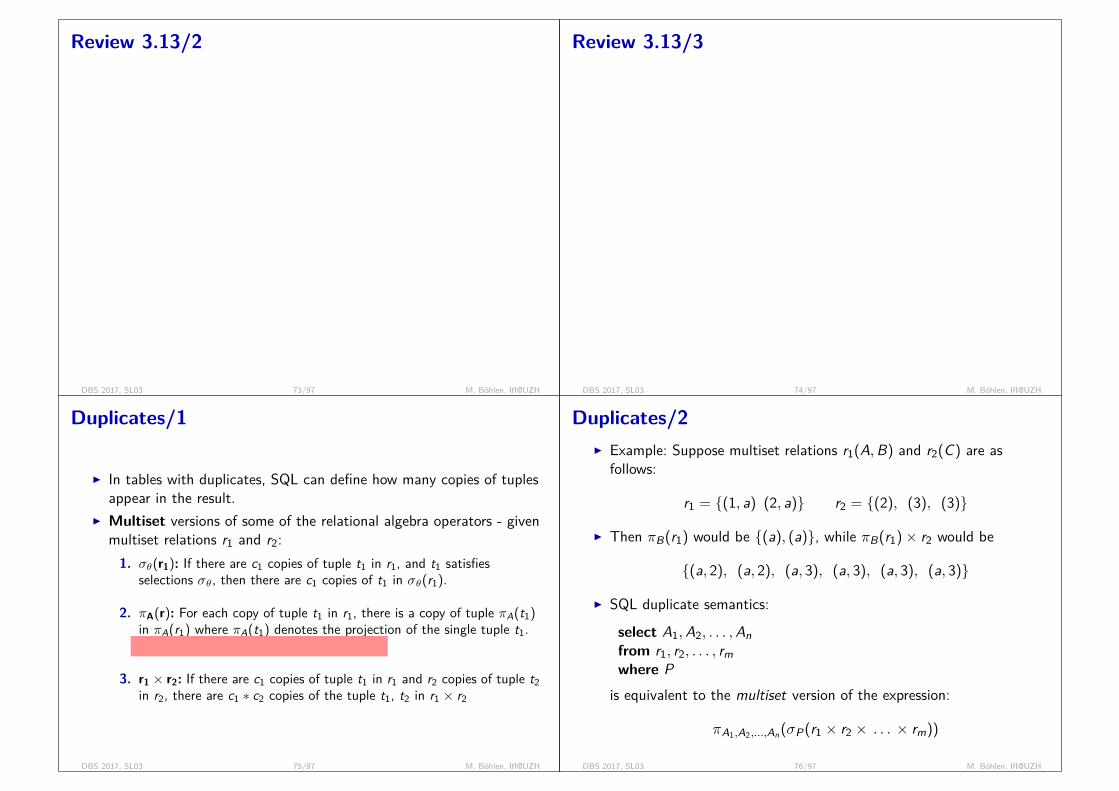
Review 3.13/2
r(N1,_) ∧ r(N2,_) ∧ N1 < N2 ∧ ∀D(r(N1,D)⇔ r(N2,D))r(N1,_) ∧ r(N2,_) ∧ N1 < N2 ∧
¬∃D(r(N1,D) ∧ r(N2,D) ∨ r(N2,D) ∧ ¬r(N1,D))
SELECT r1.N, r2.NFROM r AS r1, r AS r2WHERE r1.N < r2.NAND NOT EXISTS (SELECT *FROM r AS r3WHERE r3.N = r1.NAND NOT EXISTS (SELECT * FROM r AS r4 WHERE r4.N = r2.N AND r4.D = r3.N)UNIONSELECT *FROM r AS r3WHERE r3.N = r1.NAND NOT EXISTS (SELECT * FROM r AS r4 WHERE r4.N = r2.N AND r4.D = r3.N))
DBS 2017, SL03 73/97 M. Böhlen, IfI@UZH
Review 3.13/3
|X | = nr of degrees of X|X |+ |Y | = 2 ∗ |X ∩ Y |
X D1 Y D1X D1 Z D1Y D3 Y D1Y D3 Z D1Y D2 U D2Z D2 U D2
2 * 1 = 2 6= 1 (X) + 2 (Y)2 * 1 = 2 6= 1 (X) + 2 (Z)2 * 2 = 4 6= 2 (Y) + 2 (Z)2 * 1 = 2 6= 2 (Y) + 2 (U)2 * 1 = 2 6= 2 (Z) + 2 (U)
SELECT r1.N, r2.NFROM r AS r1, r AS r2WHERE r1.D = r2.DAND r1.N < r2.NGROUP BY r1.N, r2.NHAVING 2 * COUNT(*) = (
SELECT COUNT(*) FROM r WHERE r IN (r1.N, r2.N) )
DBS 2017, SL03 74/97 M. Böhlen, IfI@UZH
Duplicates/1
I In tables with duplicates, SQL can define how many copies of tuplesappear in the result.
I Multiset versions of some of the relational algebra operators - givenmultiset relations r1 and r2:1. σθ(r1): If there are c1 copies of tuple t1 in r1, and t1 satisfies
selections σθ, then there are c1 copies of t1 in σθ(r1).
2. πA(r): For each copy of tuple t1 in r1, there is a copy of tuple πA(t1)in πA(r1) where πA(t1) denotes the projection of the single tuple t1.
exactly the same number of tuples in πA(r) and r
3. r1 × r2: If there are c1 copies of tuple t1 in r1 and r2 copies of tuple t2in r2, there are c1 ∗ c2 copies of the tuple t1, t2 in r1 × r2
DBS 2017, SL03 75/97 M. Böhlen, IfI@UZH
Duplicates/2I Example: Suppose multiset relations r1(A,B) and r2(C) are as
follows:
r1 = {(1, a) (2, a)} r2 = {(2), (3), (3)}
I Then πB(r1) would be {(a), (a)}, while πB(r1)× r2 would be
{(a, 2), (a, 2), (a, 3), (a, 3), (a, 3), (a, 3)}
I SQL duplicate semantics:
select A1,A2, . . . ,Anfrom r1, r2, . . . , rmwhere P
is equivalent to the multiset version of the expression:
πA1,A2,...,An(σP(r1 × r2 × . . . × rm))
DBS 2017, SL03 76/97 M. Böhlen, IfI@UZH
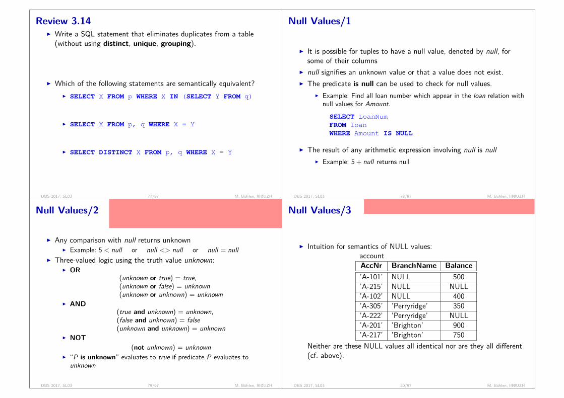
Review 3.14I Write a SQL statement that eliminates duplicates from a table
(without using distinct, unique, grouping).
impossible. logically (at SQL level) duplicates cannot be distin-guished.
I Which of the following statements are semantically equivalent?I SELECT X FROM p WHERE X IN (SELECT Y FROM q)
{{ (1), (1) }}
I SELECT X FROM p, q WHERE X = Y
{{ (1), (1), (1), (1) }}
I SELECT DISTINCT X FROM p, q WHERE X = Y
{{ (1) }}
DBS 2017, SL03 77/97 M. Böhlen, IfI@UZH
Null Values/1
I It is possible for tuples to have a null value, denoted by null, forsome of their columns
I null signifies an unknown value or that a value does not exist.I The predicate is null can be used to check for null values.
I Example: Find all loan number which appear in the loan relation withnull values for Amount.SELECT LoanNumFROM loanWHERE Amount IS NULL
I The result of any arithmetic expression involving null is nullI Example: 5 + null returns null
DBS 2017, SL03 78/97 M. Böhlen, IfI@UZH
Null Values/2
schema R(A); r(R) = {(5), (2), (NULL)};SELECT * FROM r WHERE A = 2. 1st tuple: condition evaluatesto FALSE; 2nd tuple: condition evaluates to TRUE; 3rd tuple: con-sition evaluates to UNKNOWN. {(2)} is result.
I Any comparison with null returns unknownI Example: 5 < null or null <> null or null = null
I Three-valued logic using the truth value unknown:I OR
(unknown or true) = true,(unknown or false) = unknown(unknown or unknown) = unknown
I AND(true and unknown) = unknown,(false and unknown) = false(unknown and unknown) = unknown
I NOT(not unknown) = unknown
I “P is unknown” evaluates to true if predicate P evaluates tounknown
DBS 2017, SL03 79/97 M. Böhlen, IfI@UZH
Null Values/3
show that null values are not the same. relate to example instanceshown earlier.
I Intuition for semantics of NULL values:accountAccNr BranchName Balance’A-101’ NULL 500’A-215’ NULL NULL’A-102’ NULL 400’A-305’ ’Perryridge’ 350’A-222’ ’Perryridge’ NULL’A-201’ ’Brighton’ 900’A-217’ ’Brighton’ 750
Neither are these NULL values all identical nor are they all different(cf. above).
DBS 2017, SL03 80/97 M. Böhlen, IfI@UZH
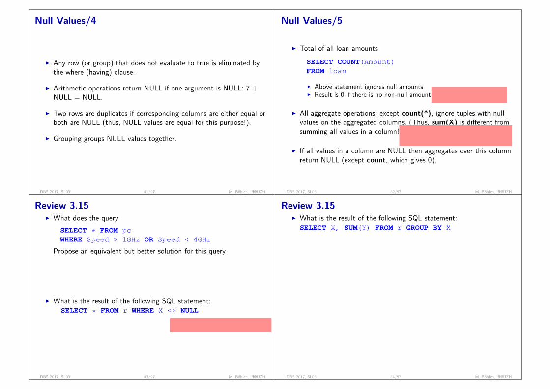
Null Values/4
I Any row (or group) that does not evaluate to true is eliminated bythe where (having) clause.
I Arithmetic operations return NULL if one argument is NULL: 7 +NULL = NULL.
I Two rows are duplicates if corresponding columns are either equal orboth are NULL (thus, NULL values are equal for this purpose!).
I Grouping groups NULL values together.
DBS 2017, SL03 81/97 M. Böhlen, IfI@UZH
Null Values/5
I Total of all loan amountsSELECT COUNT(Amount)FROM loan
I Above statement ignores null amountsI Result is 0 if there is no non-null amount
all other agg fcts (min, max,sum, avg) return NULL
I All aggregate operations, except count(*), ignore tuples with nullvalues on the aggregated columns. (Thus, sum(X) is different fromsumming all values in a column!)
exception; in principle NULL + 7 = NULL;would make aggregates cumbersome in prac-tice
I If all values in a column are NULL then aggregates over this columnreturn NULL (except count, which gives 0).
DBS 2017, SL03 82/97 M. Böhlen, IfI@UZH
Review 3.15I What does the query
SELECT * FROM pcWHERE Speed > 1GHz OR Speed < 4GHz
Propose an equivalent but better solution for this query
all PCs with a known (not null speed)SELECT * FROM pc WHERE Speed IS NOT NULL;
I What is the result of the following SQL statement:SELECT * FROM r WHERE X <> NULL
empty relation with the schema of r is not instead of <> gives expected re-sult
DBS 2017, SL03 83/97 M. Böhlen, IfI@UZH
Review 3.15I What is the result of the following SQL statement:SELECT X, SUM(Y) FROM r GROUP BY X
rX Y
NULL 52 33 4
NULL 42 2
resultX SUM(Y)2 53 4
NULL 9
exception; all NULLs are grouped together; NULLs are treated asequal for grouping
DBS 2017, SL03 84/97 M. Böhlen, IfI@UZH
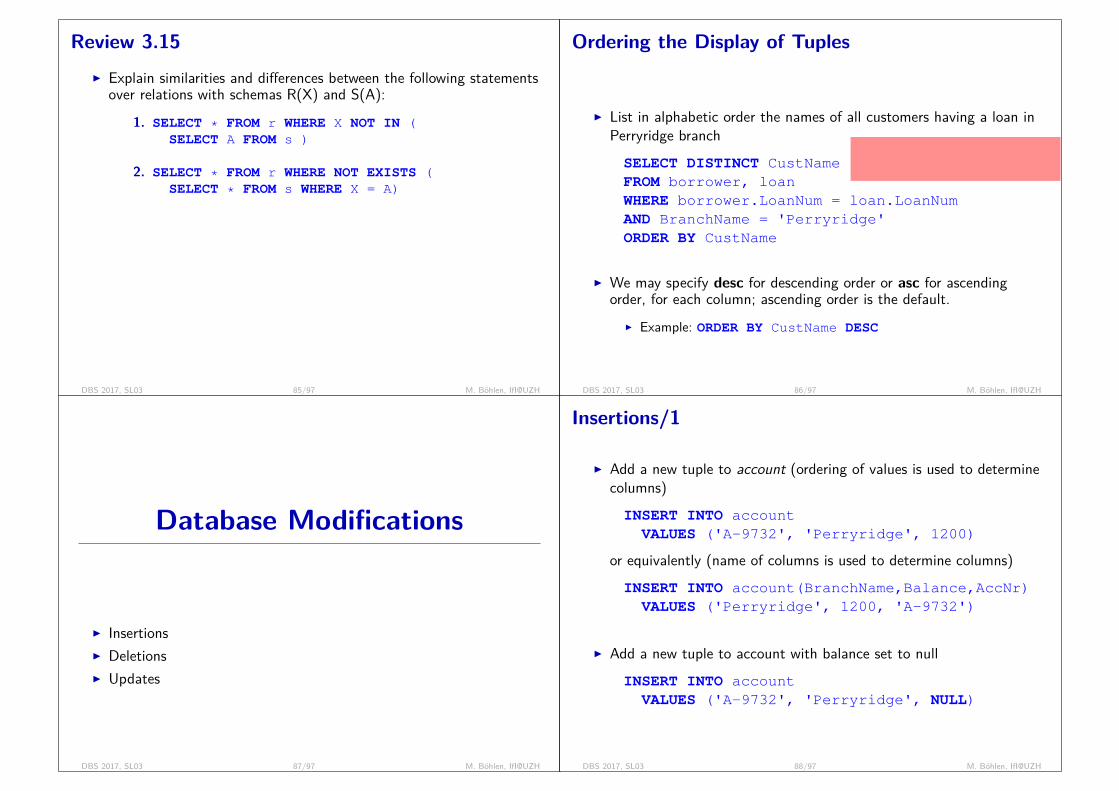
Review 3.15I Explain similarities and differences between the following statements
over relations with schemas R(X) and S(A):1. SELECT * FROM r WHERE X NOT IN (
SELECT A FROM s )
2. SELECT * FROM r WHERE NOT EXISTS (SELECT * FROM s WHERE X = A)
rX21
sX13
NULL
- identical if s does not contain null values- 1. stmt returns empty result if s contains null values- 2. stmt does not change if s contains NULL values.
DBS 2017, SL03 85/97 M. Böhlen, IfI@UZH
Ordering the Display of Tuples
order by is evaluated after the query ex-pression just before result is returned tothe application
I List in alphabetic order the names of all customers having a loan inPerryridge branchSELECT DISTINCT CustNameFROM borrower, loanWHERE borrower.LoanNum = loan.LoanNumAND BranchName = 'Perryridge'ORDER BY CustName
I We may specify desc for descending order or asc for ascendingorder, for each column; ascending order is the default.
I Example: ORDER BY CustName DESC
DBS 2017, SL03 86/97 M. Böhlen, IfI@UZH
Database Modifications
I InsertionsI DeletionsI Updates
DBS 2017, SL03 87/97 M. Böhlen, IfI@UZH
Insertions/1
I Add a new tuple to account (ordering of values is used to determinecolumns)INSERT INTO accountVALUES ('A-9732', 'Perryridge', 1200)
or equivalently (name of columns is used to determine columns)INSERT INTO account(BranchName,Balance,AccNr)VALUES ('Perryridge', 1200, 'A-9732')
I Add a new tuple to account with balance set to nullINSERT INTO accountVALUES ('A-9732', 'Perryridge', NULL)
DBS 2017, SL03 88/97 M. Böhlen, IfI@UZH

Insertions/2I Provide as a gift for all loan customers of the Perryridge branch, a
$200 savings account. Let the loan number serve as the accountnumber for the new savings accountINSERT INTO accountSELECT LoanNum, BranchName, 200FROM loanWHERE BranchName = 'Perryridge'
INSERT INTO depositorSELECT LoanNum, CustNameFROM loan, borrowerWHERE BranchName = 'Perryridge'AND loan.AccNr = borrower.AccNr
I The select from where statement is evaluated fully before any ofits results are inserted into the table.
DBS 2017, SL03 89/97 M. Böhlen, IfI@UZH
Deletions/1
I Delete all account tuples at the Perryridge branchDELETE FROM accountWHERE BranchName = 'Perryridge'
I Delete all accounts at every branch located in the city NeedhamDELETE FROM accountWHERE BranchName IN (SELECT BranchNameFROM branchWHERE BranchCity = 'Needham' )
DBS 2017, SL03 90/97 M. Böhlen, IfI@UZH
Deletions/2
I Delete the record of all accounts with balances below the average atthe bank.DELETE FROM accountWHERE Balance < ( SELECT AVG(Balance)
FROM account )
I Problem: as we delete tuples from deposit, the average balancechanges
I Solution used in SQL is the logical update semantics (guarantees thatsequence in which updates to a table are computed does not matter):1. First, compute avg balance and find all tuples to delete2. Next, delete all tuples found above (without recomputing avg or
evaluating the condition again)
DBS 2017, SL03 91/97 M. Böhlen, IfI@UZH
Updates/1
I Increase all accounts with balances over $10,000 by 6%, all otheraccounts receive 5%.
I Write two update statements:UPDATE accountSET Balance = Balance * 1.06WHERE Balance > 10000
UPDATE accountSET Balance = Balance * 1.05WHERE Balance <= 10000
I The order is importantI Can be done better using the case statement (next slide)
DBS 2017, SL03 92/97 M. Böhlen, IfI@UZH
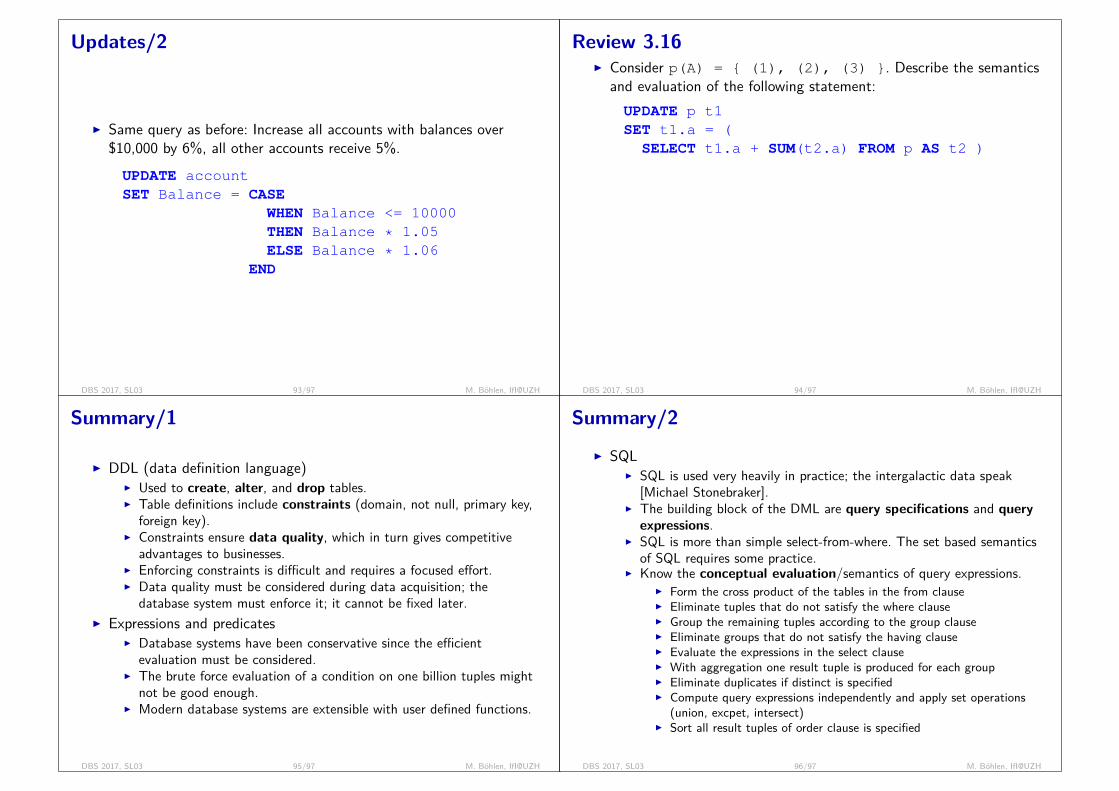
Updates/2
I Same query as before: Increase all accounts with balances over$10,000 by 6%, all other accounts receive 5%.UPDATE accountSET Balance = CASE
WHEN Balance <= 10000THEN Balance * 1.05ELSE Balance * 1.06
END
DBS 2017, SL03 93/97 M. Böhlen, IfI@UZH
Review 3.16I Consider p(A) = { (1), (2), (3) }. Describe the semantics
and evaluation of the following statement:UPDATE p t1SET t1.a = (SELECT t1.a + SUM(t2.a) FROM p AS t2 )
- correlated subquery is evaluated for each row of outer relation;changes are first determined and then applied
- 1st row: 1 will be updated to 7 (= 1+6)- 2nd row: 2 will be updated to 8 (= 2+6)- 3rd row: 3 will be updated to 9 (= 3+6)
- result = {(7), (8), (9)}
DBS 2017, SL03 94/97 M. Böhlen, IfI@UZH
Summary/1
I DDL (data definition language)I Used to create, alter, and drop tables.I Table definitions include constraints (domain, not null, primary key,
foreign key).I Constraints ensure data quality, which in turn gives competitive
advantages to businesses.I Enforcing constraints is difficult and requires a focused effort.I Data quality must be considered during data acquisition; the
database system must enforce it; it cannot be fixed later.I Expressions and predicates
I Database systems have been conservative since the efficientevaluation must be considered.
I The brute force evaluation of a condition on one billion tuples mightnot be good enough.
I Modern database systems are extensible with user defined functions.
DBS 2017, SL03 95/97 M. Böhlen, IfI@UZH
Summary/2I SQL
I SQL is used very heavily in practice; the intergalactic data speak[Michael Stonebraker].
I The building block of the DML are query specifications and queryexpressions.
I SQL is more than simple select-from-where. The set based semanticsof SQL requires some practice.
I Know the conceptual evaluation/semantics of query expressions.I Form the cross product of the tables in the from clauseI Eliminate tuples that do not satisfy the where clauseI Group the remaining tuples according to the group clauseI Eliminate groups that do not satisfy the having clauseI Evaluate the expressions in the select clauseI With aggregation one result tuple is produced for each groupI Eliminate duplicates if distinct is specifiedI Compute query expressions independently and apply set operations
(union, excpet, intersect)I Sort all result tuples of order clause is specified
DBS 2017, SL03 96/97 M. Böhlen, IfI@UZH
Summary/3
I The difference between set and multisets (or bags) is relevant.I Subqueries are natural and help the understanding; it is possible
(and advisable) to only use exists and not exists.I Large parts of RA, SQL and DRC are equivalent; know how to go
from one to the other.I Modification statements use the logical update semantics
(compute changes before they are applied).I The SQL OLAP extensions (cf. Data Warehouse course) further
extend SQL to better support report generation (cross tabs, movingaverages, etc).
DBS 2017, SL03 97/97 M. Böhlen, IfI@UZH

Reviews: 9 12 33 37 39 59
Database SystemsSpring 2017
Database ProgrammingSL04
I ViewsI Recursive QueriesI Integrity ConstraintsI Functions and Procedural ConstructsI TriggersI Accessing Databases
issues that are important in ap-plications and real systemsconnecting DBMS with applica-tionsembedding DBMS into applica-tions
DBS 2017, SL04 1/66 M. Böhlen, IfI@UZH
Literature and Acknowledgments
Reading List for SL04:I Database Systems, Chapters 5 (5.2 and 5.3) and 12, Sixth Edition,
Ramez Elmasri and Shamkant B. Navathe, Pearson Education, 2010.
These slides were developed by:I Michael Böhlen, University of Zürich, SwitzerlandI Johann Gamper, Free University of Bozen-Bolzano, Italy
The slides are based on the following text books and associated material:I Fundamentals of Database Systems, Fourth Edition, Ramez Elmasri
and Shamkant B. Navathe, Pearson Addison Wesley, 2004.I A. Silberschatz, H. Korth, and S. Sudarshan: Database System
Concepts, McGraw Hill, 2006.
DBS 2017, SL04 2/66 M. Böhlen, IfI@UZH
Views
I Purpose of viewsI Creation and use of viewsI Handling views in the DBMSI Temporary views
DBS 2017, SL04 3/66 M. Böhlen, IfI@UZH
Views/1I A view is a table whose rows are not stored in the database. The
rows are computed when needed from the view definition.I This is useful in cases where
I it is not desirable for all users to see the entire logical model (that is,all the actual tables stored in the database), or
I the user wants to access computed results (rather than the actualdata stored on the disk)
I Consider a person who needs to know a customer’s name, loannumber and branch name, but has no need to see the loan amount.This person should see a relation described, in SQL, bySELECT CustName, borrower.LoanNr, BranchNameFROM borrower, loanWHERE borrower.LoanNr = loan.LoanNr
I A view provides a mechanism to hide data from the view of users, orto give users direct access to the results of (complex) computations.
DBS 2017, SL04 4/66 M. Böhlen, IfI@UZH

Views/2
I A view is defined using the create view statement which has theform
CREATE VIEW v AS <query expression>
where <query expression> is any legal SQL expression. The viewname is represented by v .
I Once a view is defined, the view name can be used to refer to thevirtual relation that the view generates.
I When a view is created, the query expression is stored in thedatabase.
I Any table that is not of the conceptual model but is made visible toa user as a “virtual table” is called a view.
DBS 2017, SL04 5/66 M. Böhlen, IfI@UZH
Views/3I A view consisting of branches and their customers:
CREATE VIEW allCustomer AS( SELECT BranchName, CustNameFROM depositor, accountWHERE depositor.AccNr = account.AccNr )
UNION( SELECT BranchName, CustNameFROM borrower, loanWHERE borrower.LoanNr = loan.LoanNr )
I Find all customers of the Perryridge branch:SELECT CustNameFROM allCustomerWHERE branche_name = 'Perryridge'
DBS 2017, SL04 6/66 M. Böhlen, IfI@UZH
Views/4
I The view definition is stored in the meta database.
cheap. several 1000views are OK.
I The meaning of a query expression that includes views is definedthrough view expansion.
I The view expansion of an expression repeats the followingreplacement step:
repeatFind any view vi in e1;Replace view vi by the expression defining vi ;
until no more views are present in e1I As long as the view definitions are not recursive, this loop will
terminate
DBS 2017, SL04 7/66 M. Böhlen, IfI@UZH
Views/5
I Tables and views can be used interchangeably in queries.
I Tables and views behave differently wrt modification operations.I Updates to views are restricted. No broad consensus/standard exists
and DBMSs behave differently.I Roughly, a view shall be updatable if the database system can
determine the reverse mapping from the view schema to the schemaof the underlying base tables.
I The exact definition of updatable views has been enlargedsignificantly from SQL-1992 to SQL:1999 (cf. below).
DBS 2017, SL04 8/66 M. Böhlen, IfI@UZH
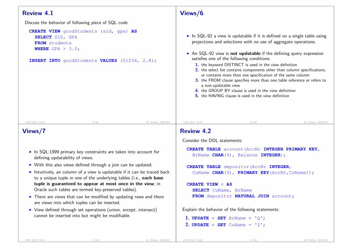
Review 4.1Discuss the behavior of following piece of SQL code.CREATE VIEW goodStudents (sid, gpa) ASSELECT SID, GPAFROM studentsWHERE GPA > 3.0;
INSERT INTO goodStudents VALUES (51234, 2.8);
I result: student with SID 51234 and GPA 2.8 is inserted intostudents
I student cannot be retrieved through view goodStudentsI SQL allows thisI WITH CHECK OPTION can be added to the view definition to
disallow insertion (only allows insertions that can be retrievedthrough the view
DBS 2017, SL04 9/66 M. Böhlen, IfI@UZH
Views/6
I In SQL-92 a view is updatable if it is defined on a single table usingprojections and selections with no use of aggregate operations.
I An SQL-92 view is not updatable if the defining query expressionsatisfies one of the following conditions:1. the keyword DISTINCT is used in the view definition2. the select list contains components other than column specifications,
or contains more than one specification of the same column3. the FROM clause specifies more than one table reference or refers to
a non-updatable view4. the GROUP BY clause is used in the view definition5. the HAVING clause is used in the view definition
DBS 2017, SL04 10/66 M. Böhlen, IfI@UZH
Views/7
I In SQL:1999 primary key constraints are taken into account fordefining updatability of views.
I With this also views defined through a join can be updated.I Intuitively, an column of a view is updatable if it can be traced back
to a unique tuple in one of the underlying tables (i.e., each basetuple is guaranteed to appear at most once in the view; inOracle such tables are termed key-preserved tables).
I There are views that can be modified by updating rows and thereare views into which tuples can be inserted.
I View defined through set operations (union, except, intersect)cannot be inserted into but might be modifiable.
DBS 2017, SL04 11/66 M. Böhlen, IfI@UZH
Review 4.2Consider the DDL statements:CREATE TABLE account(AccNr INTEGER PRIMARY KEY,BrName CHAR(9), Balance INTEGER);
CREATE TABLE depositor(AccNr INTEGER,CuName CHAR(9), PRIMARY KEY(AccNr,CuName));
CREATE VIEW v ASSELECT CuName, BrNameFROM depositor NATURAL JOIN account;
Explain the behavior of the following statements:1. UPDATE v SET BrName = 'Q';
2. UPDATE v SET CuName = 'Z';
DBS 2017, SL04 12/66 M. Böhlen, IfI@UZH

Review 4.2
1. not allowed in SQL
account123 P 5456 D 6
depositor123 X123 Y456 X
vX PY PX D
2. allowed in SQL
account123 P 5456 D 6
depositor123 X123 Y456 X
vX PY PX D
CuName can be updated (sinceit derives from one base tuple;BrName cannot be updated)
DBS 2017, SL04 13/66 M. Böhlen, IfI@UZH
With Clause/1I The with clause provides a way of defining temporary views whose
definition is available only to the query in which the with clauseoccurs.
I The with clause is useful to structure complex SQL statements andeliminate code repetitions.
I Find all accounts with the maximum balanceWITHmaxBalance(Val) AS (SELECT MAX(Balance)FROM account
)SELECT AccNrFROM account, maxBalanceWHERE account.Balance = maxBalance.Val
defines local and temporaryview maxBalance(Val); goodfor structuring code; avoidsrepetitions of view definition.
DBS 2017, SL04 14/66 M. Böhlen, IfI@UZH
With Clause/2I Find all branches where the total account deposit is greater than the
average of the total account deposits at all branches.WITHbraTot(BranchName,Val) AS (SELECT BranchName, SUM(Balance)FROM accountGROUP BY BranchName
),braTotAvg(Val) AS (SELECT AVG(Val)FROM braTot
)SELECT BranchNameFROM braTot, braTotAvgWHERE braTot.Val > braTotAvg.Val
DBS 2017, SL04 15/66 M. Böhlen, IfI@UZH
Recursion in SQL
I Recursive views in SQL-1999I Example of a recursive view
DBS 2017, SL04 16/66 M. Böhlen, IfI@UZH

Recursion in SQL/1
fac(X) ={
1 n = 1n ∗ fac(n − 1) n > 1
I SQL:1999 permits recursive view definitionI Example: find all employee-manager pairs, where the employee
reports to the manager directly or indirectly (that is manager’smanager, manager’s manager’s manager, etc.)
WITH RECURSIVE mgr(EmpName,MgrName ) AS (SELECT EmpName, BossNameFROM emplUNIONSELECT empl.EmpName, mgr.MgrNameFROM empl, mgrWHERE BossName = mgr.EmpName
)SELECT * FROM mgr;
View mgr is the transitive closure of the empl relation.
recursive case
base case
DBS 2017, SL04 17/66 M. Böhlen, IfI@UZH
Recursion in SQL/2
I Recursive views make it possible to write queries, such as transitiveclosure queries, that cannot be written without recursion oriteration.
I Intuition: Without recursion, a non-recursive non-iterative programcan perform only a fixed number of joins of empl with itself
I This can give only a fixed number of levels of managers.I We can always construct a database with a greater number of levels
of managers than a fixed number.
I Computing transitive closureI The next slide shows a empl relationI Each step of the iterative process constructs an extended version of
mgr from its recursive definition.I The final result is called the fixpoint of the recursive view definition.
DBS 2017, SL04 18/66 M. Böhlen, IfI@UZH
Example of Fixpoint Computation/1
Klinger
Jones Rensal
Estovar Duarte
Barinsky Corbin
Alon
emplEmpName BossName’Alon’ ’Barinsky’’Barinsky’ ’Estovar’’Corbin’ ’Duarte’’Duarte’ ’Jones’’Estovar’ ’Jones’’Jones’ ’Klinger’’Rensal’ ’Klinger’
DBS 2017, SL04 19/66 M. Böhlen, IfI@UZH
Example of Fixpoint Computation/2
mgrEmpName MgrName’Alon’ ’Barinsky’’Barinsky’ ’Estovar’’Corbin’ ’Duarte’
direct mgrs (1 step)
’Duarte’ ’Jones’’Estovar’ ’Jones’’Jones’ ’Klinger’’Rensal’ ’Klinger’’Alon’ ’Estovar’’Barinsky’ ’Jones’
indirect mgrs (2 steps)
’Corbin’ ’Jones’’Duarte’ ’Klinger’’Estovar’ ’Klinger’’Alon’ ’Jones’’Barinsky’ ’Klinger’
indirect mgrs (3 steps)
’Corbin’ ’Klinger’’Alon’ ’Klinger’
Klinger
Jones Rensal
Estovar Duarte
Barinsky Corbin
Alon
DBS 2017, SL04 20/66 M. Böhlen, IfI@UZH
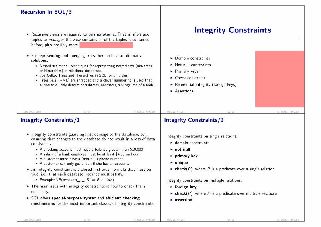
Recursion in SQL/3
I Recursive views are required to be monotonic. That is, if we addtuples to manager the view contains all of the tuples it containedbefore, plus possibly more.
no negation (not exists, except, ...)
I For representing and querying trees there exist also alternativesolutions:
I Nested set model: techniques for representing nested sets (aka treesor hierarchies) in relational databases.
I Joe Celko: Trees and Hierarchies in SQL for SmartiesI Trees (e.g., XML) are shredded and a clever numbering is used that
allows to quickly determine subtrees, ancestors, siblings, etc of a node.
DBS 2017, SL04 21/66 M. Böhlen, IfI@UZH
Integrity Constraints
I Domain constraintsI Not null constraintsI Primary keysI Check constraintI Referential integrity (foreign keys)I Assertions
Real world: there are alwaysexceptions; integrity constraintsare never satisfied to 100%
data quality is a company-wide task; understanding for thismust be established
databases help to enforce gooddata quality (through integrityconstraints
technically: integrity constraintsare very expensive (expensivechecks when adding data)
DBS 2017, SL04 22/66 M. Böhlen, IfI@UZH
Integrity Constraints/1
I Integrity constraints guard against damage to the database, byensuring that changes to the database do not result in a loss of dataconsistency.
I A checking account must have a balance greater than $10,000I A salary of a bank employee must be at least $4.00 an hour.I A customer must have a (non-null) phone number.I A customer can only get a loan if she has an account.
I An integrity constraint is a closed first order formula that must betrue, i.e., that each database instance must satisfy.
I Example: ∀B(account(_,_,B) ⇒ B < 10M)I The main issue with integrity constraints is how to check them
efficiently.I SQL offers special-purpose syntax and efficient checkingmechanisms for the most important classes of integrity constraints.
DBS 2017, SL04 23/66 M. Böhlen, IfI@UZH
Integrity Constraints/2
Integrity constraints on single relations:I domain constraintsI not nullI primary keyI uniqueI check(P), where P is a predicate over a single relation
Integrity constraints on multiple relations:I foreign keyI check(P), where P is a predicate over multiple relationsI assertion
DBS 2017, SL04 24/66 M. Böhlen, IfI@UZH

Domain Constraints
I Domain constraints are the most elementary form of integrityconstraints. They check values inserted in the database, and theycheck queries to ensure that the comparisons make sense.
I New domains can be created from existing data typesI Example:
CREATE DOMAIN Dollars INTEGERCREATE DOMAIN Pounds INTEGER
I We cannot assign or compare a value of type Dollars to a value oftype Pounds.
I However, we can convert values of type Dollar as follows:CAST(r.Amnt/1.5 AS Pounds)
DBS 2017, SL04 25/66 M. Böhlen, IfI@UZH
Not Null Constraint
I Declare BranchName to be not null:BranchName CHAR(15) NOT NULL
I Declare the domain Dollars to be not null:CREATE DOMAIN Dollars INTEGER NOT NULL
DBS 2017, SL04 26/66 M. Böhlen, IfI@UZH
Primary Key
I A primary key ensures that an attribute value is not null and uniqueacross all rows of a table. Therefore it can be used to identify aunique row in a table, and is used for query optimization.
I Primary and candidate keys and foreign keys can be specified as partof the SQL create table statement:
I The primary key clause lists attributes that form the primary key.I Example:
CREATE TABLE customer (CustName CHAR(20),CustStreet CHAR(30),CustCity CHAR(30),PRIMARY KEY (CustName) )
DBS 2017, SL04 27/66 M. Böhlen, IfI@UZH
The Unique Constraint
a unique constraint provides aperformance guarantee. result ofa join is of size n and not n2. da-tabase system can use knowled-ge about unique attribute valuesto automatically create indexes
I unique (A1,A2, . . . ,Am)I The unique specification states that the attributes
A1,A2, . . . ,Amform a candidate key.
I Candidate keys are permitted to be null (in contrast to primarykeys).
DBS 2017, SL04 28/66 M. Böhlen, IfI@UZH
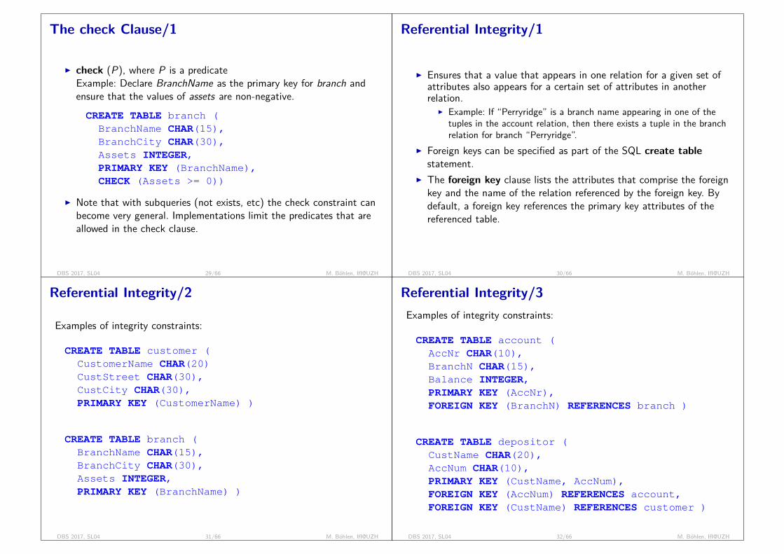
The check Clause/1
I check (P), where P is a predicateExample: Declare BranchName as the primary key for branch andensure that the values of assets are non-negative.CREATE TABLE branch (BranchName CHAR(15),BranchCity CHAR(30),Assets INTEGER,PRIMARY KEY (BranchName),CHECK (Assets >= 0))
I Note that with subqueries (not exists, etc) the check constraint canbecome very general. Implementations limit the predicates that areallowed in the check clause.
DBS 2017, SL04 29/66 M. Böhlen, IfI@UZH
Referential Integrity/1
I Ensures that a value that appears in one relation for a given set ofattributes also appears for a certain set of attributes in anotherrelation.
I Example: If “Perryridge” is a branch name appearing in one of thetuples in the account relation, then there exists a tuple in the branchrelation for branch “Perryridge”.
I Foreign keys can be specified as part of the SQL create tablestatement.
I The foreign key clause lists the attributes that comprise the foreignkey and the name of the relation referenced by the foreign key. Bydefault, a foreign key references the primary key attributes of thereferenced table.
DBS 2017, SL04 30/66 M. Böhlen, IfI@UZH
Referential Integrity/2
Examples of integrity constraints:
CREATE TABLE customer (CustomerName CHAR(20)CustStreet CHAR(30),CustCity CHAR(30),PRIMARY KEY (CustomerName) )
CREATE TABLE branch (BranchName CHAR(15),BranchCity CHAR(30),Assets INTEGER,PRIMARY KEY (BranchName) )
DBS 2017, SL04 31/66 M. Böhlen, IfI@UZH
Referential Integrity/3Examples of integrity constraints:
CREATE TABLE account (AccNr CHAR(10),BranchN CHAR(15),Balance INTEGER,PRIMARY KEY (AccNr),FOREIGN KEY (BranchN) REFERENCES branch )
CREATE TABLE depositor (CustName CHAR(20),AccNum CHAR(10),PRIMARY KEY (CustName, AccNum),FOREIGN KEY (AccNum) REFERENCES account,FOREIGN KEY (CustName) REFERENCES customer )
DBS 2017, SL04 32/66 M. Böhlen, IfI@UZH

Review 4.3Assume tables p(X) and q(Y). p.X is a primary key. q.Y is a foreign keythat references p.X.1. Use a check constraint to formulate the foreign key constraint.2. Formulate a query that returns an empty result if the foreign key is
satisfied and a non-empty result otherwise.
IC: ∀A(q(A) ⇒ p(A))rewritten IC: ¬∃A(q(A) ∧ ¬p(A))
CHECK (NOT EXISTS (SELECT *FROM qWHERE NOT EXISTS (SELECT *FROM pWHERE X = Y )))
SELECT *FROM qWHERE NOT EXISTS (
SELECT *FROM pWHERE X = Y )
DBS 2017, SL04 33/66 M. Böhlen, IfI@UZH
Assertions/1
I An assertion is a predicate expressing a condition that the databasemust satisfy.
I An assertion in SQL takes the formcreate assertion <assertion-name> check <predicate>
I When an assertion is made, the system tests it for validity, and testsit again on every update that might violate the assertion.
I This testing may introduce a significant amount of overhead; henceassertions should be used with care.
I Asserting∀X (p(X ))
is achieved using¬∃¬(p(X ))
DBS 2017, SL04 34/66 M. Böhlen, IfI@UZH
Assertion/2
I Every loan has at least one borrower who maintains an account witha minimum balance or $1000CREATE ASSERTION balance_constraint CHECKNOT EXISTS (SELECT *FROM loanWHERE NOT EXISTS (SELECT *FROM borrower b, depositor d, account aWHERE loan.LoanNr = b.LoanNrAND b.CustName = d.CustNameAND d.AccNr = a.AccNrAND a.Balance >= 1000)))
DBS 2017, SL04 35/66 M. Böhlen, IfI@UZH
Assertion/3
I The sum of all loan amounts for each branch must be less than thesum of all account balances at the branch.CREATE ASSERTION sum_constraint CHECK (NOT EXISTS (SELECT *FROM branch bWHERE( SELECT SUM(Amount)FROM loan lWHERE l.BranchName = b.BranchName )
>=( SELECT SUM(Balance)FROM account aWHERE l.BranchName = b.BranchName )))
DBS 2017, SL04 36/66 M. Böhlen, IfI@UZH

Review 4.4/1Consider the tablesCREATE TABLE branch(BranchName CHAR(9),BranchCity CHAR(9), Assets INTEGER);
CREATE TABLE account(AccNr INTEGER PRIMARY KEY,BranchName CHAR(9), Balance INTEGER);
Explain how to efficiently check the integrity constraint
∀BN(account(_,BN,_) ⇒ branch(BN,_,_))
by considering the different database modifications.
db is consistent before a modification operation is performed (dbmsensures that db is never in an inconsistent state)thus, dbms must only check ICs that are affected by the modification;rewrite (specialize) ICs s.t. they incorporate the modification.
DBS 2017, SL04 37/66 M. Böhlen, IfI@UZH
Review 4.4/2
Rewrite ∀X (a(_,X ,_) ⇒ b(X ,_,_)) to ∀X (¬a(_,X ,_) ∨ b(X ,_,_)).
For ∀X (¬a(_,X ,_) ∨ b(X ,_,_)) only changes to a and b are relevant.
I addition of a(_,’P’,_): check if b(’P’,_,_) is true (present in DB)I deletion of a(_,’P’,_): OK (no check needed)I addition of b(’P’,_,_): OK (no check needed)I deletion of b(’P’,_,_): check if a(_,’P’,_) is false (not present in DB)
DBS 2017, SL04 38/66 M. Böhlen, IfI@UZH
Review 4.5Create a table for cities and a table for states. For each state its capitalshall be recorded and for each city the state it is located in shall berecorded. Discuss the properties of the following solution:
CREATE TABLE cities(CName CHAR(9) PRIMARY KEY, State CHAR(9));CREATE TABLE states(SName CHAR(9) PRIMARY KEY, Capital CHAR(9));ALTER TABLE cities ADD FOREIGN KEY (State) REFERENCES states(SName);ALTER TABLE states ADD FOREIGN KEY (Capital) REFERENCES cities(CName);
neither a city nor a state can be added independently. multiple tuplesmust be added before ICs can be checked.
I transactions = multiple SQL stmts as one unitI DBMSs do eager checking (after each modification) if possible
to improve performanceI DEFERRABLE INITIALLY DEFERRED can/must be added
to FK.
DBS 2017, SL04 39/66 M. Böhlen, IfI@UZH
User Defined Functions
I PL/pgSQL value functionsI PL/pgSQL table functionsI External language functions
DBS 2017, SL04 40/66 M. Böhlen, IfI@UZH
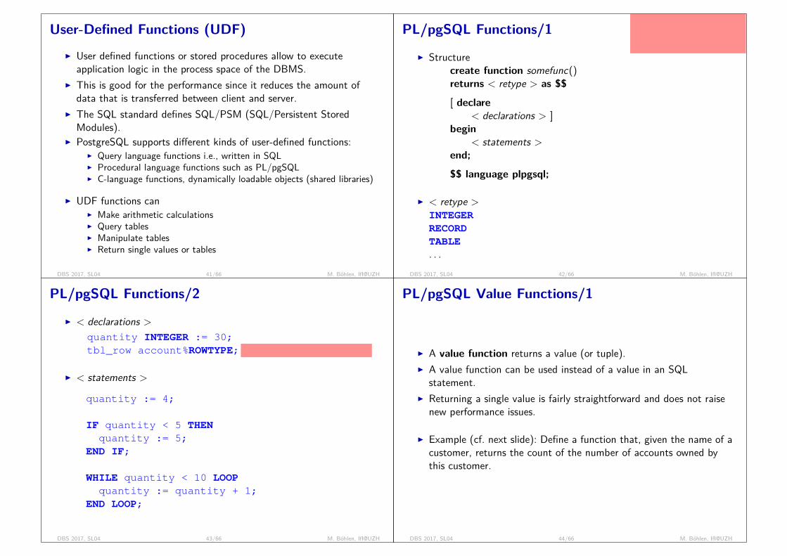
User-Defined Functions (UDF)I User defined functions or stored procedures allow to execute
application logic in the process space of the DBMS.I This is good for the performance since it reduces the amount of
data that is transferred between client and server.I The SQL standard defines SQL/PSM (SQL/Persistent Stored
Modules).I PostgreSQL supports different kinds of user-defined functions:
I Query language functions i.e., written in SQLI Procedural language functions such as PL/pgSQLI C-language functions, dynamically loadable objects (shared libraries)
I UDF functions canI Make arithmetic calculationsI Query tablesI Manipulate tablesI Return single values or tables
DBS 2017, SL04 41/66 M. Böhlen, IfI@UZH
PL/pgSQL Functions/1
goal is to show the main con-cepts; there is an exercise withfunctions; details of the syntaxare not the key part
I Structurecreate function somefunc()returns < retype > as $$
[ declare< declarations > ]
begin< statements >
end;
$$ language plpgsql;
I < retype >INTEGERRECORDTABLE. . .
DBS 2017, SL04 42/66 M. Böhlen, IfI@UZH
PL/pgSQL Functions/2
I < declarations >
quantity INTEGER := 30;tbl_row account%ROWTYPE;
tuple with schema of table account
I < statements >
quantity := 4;
IF quantity < 5 THENquantity := 5;
END IF;
WHILE quantity < 10 LOOPquantity := quantity + 1;
END LOOP;
DBS 2017, SL04 43/66 M. Böhlen, IfI@UZH
PL/pgSQL Value Functions/1
I A value function returns a value (or tuple).I A value function can be used instead of a value in an SQL
statement.I Returning a single value is fairly straightforward and does not raise
new performance issues.
I Example (cf. next slide): Define a function that, given the name of acustomer, returns the count of the number of accounts owned bythis customer.
DBS 2017, SL04 44/66 M. Böhlen, IfI@UZH
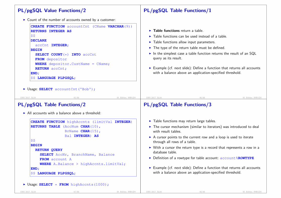
PL/pgSQL Value Functions/2I Count of the number of accounts owned by a customer:
CREATE FUNCTION accountCnt (CName VARCHAR(9))RETURNS INTEGER AS$$DECLAREaccCnt INTEGER;
BEGINSELECT COUNT(*) INTO accCntFROM depositorWHERE depositor.CustName = CName;RETURN accCnt;
END;$$ LANGUAGE PLPGSQL;
I Usage: SELECT accountCnt('Bob');
DBS 2017, SL04 45/66 M. Böhlen, IfI@UZH
PL/pgSQL Table Functions/1
I Table functions return a table.I Table functions can be used instead of a table.I Table functions allow input parameters.I The type of the return table must be defined.I In the simplest case a table function returns the result of an SQL
query as its result.
I Example (cf. next slide): Define a function that returns all accountswith a balance above an application-specified threshold.
DBS 2017, SL04 46/66 M. Böhlen, IfI@UZH
PL/pgSQL Table Functions/2I All accounts with a balance above a threshold:
CREATE FUNCTION highAccnts (limitVal INTEGER)RETURNS TABLE (AccNum CHAR(10),
BrName CHAR(15),Bal INTEGER) AS
$$BEGINRETURN QUERYSELECT AccNr, BranchName, BalanceFROM account AWHERE A.Balance > highAccnts.limitVal;
END;$$ LANGUAGE PLPGSQL;
I Usage: SELECT * FROM highAccnts(1000);
DBS 2017, SL04 47/66 M. Böhlen, IfI@UZH
PL/pgSQL Table Functions/3
I Table functions may return large tables.I The cursor mechanism (similar to iterators) was introduced to deal
with result tables.I A cursor points to the current row and a loop is used to iterate
through all rows of a table.I With a cursor the return type is a record that represents a row in a
database table.I Definition of a rowtype for table account: account%ROWTYPE
I Example (cf. next slide): Define a function that returns all accountswith a balance above an application-specified threshold.
DBS 2017, SL04 48/66 M. Böhlen, IfI@UZH
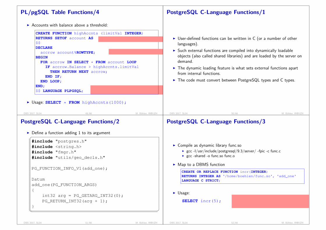
PL/pgSQL Table Functions/4
code is terrible in terms of performance; scan oftable; query optimization is disabled
I Accounts with balance above a threshold:CREATE FUNCTION highAccnts (limitVal INTEGER)RETURNS SETOF account AS$$DECLARE
accrow account%ROWTYPE;BEGIN
FOR accrow IN SELECT * FROM account LOOPIF accrow.Balance > highAccnts.limitVal
THEN RETURN NEXT accrow;END IF;
END LOOP;END;$$ LANGUAGE PLPGSQL;
I Usage: SELECT * FROM highAccnts(1000);
set of tuples with schema of table account
tuple with schema of table account
DBS 2017, SL04 49/66 M. Böhlen, IfI@UZH
PostgreSQL C-Language Functions/1
I User-defined functions can be written in C (or a number of otherlanguages).
I Such external functions are compiled into dynamically loadableobjects (also called shared libraries) and are loaded by the server ondemand.
I The dynamic loading feature is what sets external functions apartfrom internal functions.
I The code must convert between PostgreSQL types and C types.
DBS 2017, SL04 50/66 M. Böhlen, IfI@UZH
PostgreSQL C-Language Functions/2
I Define a function adding 1 to its argument�#include "postgres.h"#include <string.h>#include "fmgr.h"#include "utils/geo_decls.h"
PG_FUNCTION_INFO_V1(add_one);
Datumadd_one(PG_FUNCTION_ARGS){
int32 arg = PG_GETARG_INT32(0);PG_RETURN_INT32(arg + 1);
}� �DBS 2017, SL04 51/66 M. Böhlen, IfI@UZH
PostgreSQL C-Language Functions/3
func.so is name of library (.so .ddl)
add_one is name of external function in this library
I Compile as dynamic library func.soI gcc -I/usr/include/postgresql/9.3/server/ -fpic -c func.cI gcc -shared -o func.so func.o
I Map to a DBMS functionCREATE OR REPLACE FUNCTION incr(INTEGER)RETURNS INTEGER AS '/home/boehlen/func.so', 'add_one'LANGUAGE C STRICT;
I Usage:SELECT incr(5);
DBS 2017, SL04 52/66 M. Böhlen, IfI@UZH
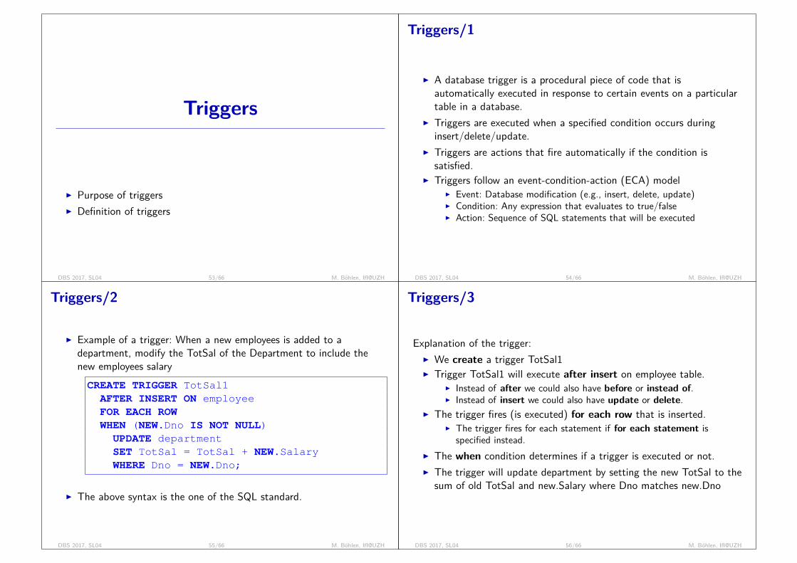
Triggers
I Purpose of triggersI Definition of triggers
DBS 2017, SL04 53/66 M. Böhlen, IfI@UZH
Triggers/1
I A database trigger is a procedural piece of code that isautomatically executed in response to certain events on a particulartable in a database.
I Triggers are executed when a specified condition occurs duringinsert/delete/update.
I Triggers are actions that fire automatically if the condition issatisfied.
I Triggers follow an event-condition-action (ECA) modelI Event: Database modification (e.g., insert, delete, update)I Condition: Any expression that evaluates to true/falseI Action: Sequence of SQL statements that will be executed
DBS 2017, SL04 54/66 M. Böhlen, IfI@UZH
Triggers/2
I Example of a trigger: When a new employees is added to adepartment, modify the TotSal of the Department to include thenew employees salaryCREATE TRIGGER TotSal1AFTER INSERT ON employeeFOR EACH ROWWHEN (NEW.Dno IS NOT NULL)UPDATE departmentSET TotSal = TotSal + NEW.SalaryWHERE Dno = NEW.Dno;
I The above syntax is the one of the SQL standard.
DBS 2017, SL04 55/66 M. Böhlen, IfI@UZH
Triggers/3
Explanation of the trigger:I We create a trigger TotSal1I Trigger TotSal1 will execute after insert on employee table.
I Instead of after we could also have before or instead of.I Instead of insert we could also have update or delete.
I The trigger fires (is executed) for each row that is inserted.I The trigger fires for each statement if for each statement is
specified instead.I The when condition determines if a trigger is executed or not.I The trigger will update department by setting the new TotSal to the
sum of old TotSal and new.Salary where Dno matches new.Dno
DBS 2017, SL04 56/66 M. Böhlen, IfI@UZH

Triggers/4I In PostgreSQL a trigger consist of two parts:
I A trigger function that defines the action to be performedI A trigger that defines when the trigger must be fired.
I A trigger function must return NULL or a row with the schema ofthe table the trigger was fired for.
CREATE OR REPLACE FUNCTION checkTemp()RETURNS TRIGGER AS$$DECLAREBEGINIF NEW.val < -273 THENRAISE EXCEPTION 'invalid value: %', NEW.val;
END IFRETURN NEW;
END;$$ LANGUAGE PLPGSQL;
DBS 2017, SL04 57/66 M. Böhlen, IfI@UZH
Triggers/5
PostgreSQL trigger:I A trigger is associated with a table or view and executes the
specified function when certain events occur.I A trigger can fire before the operation, after the operation has
completed, or instead of the operation.I A trigger can fire for each row or for each statement.
A PostgreSQL example of a trigger definition.CREATE TRIGGER TrigTempCheckBEFORE INSERT OR UPDATEON temperatureFOR EACH ROWEXECUTE PROCEDURE checkTemp();
DBS 2017, SL04 58/66 M. Böhlen, IfI@UZH
Review 4.6Compare triggers and integrity constraints.
triggers:I + powerful (action can be specified); useful to do things that
are otherwise not possibleI + control of steps of processingI + easy to implementI - difficult to maintain for userI - procedural; sequence of execution is relevant
integrity constraints:I + clean concept; checks state of a databaseI + declarative; order of processing not relevantI + easy to maintain (for user)I - difficult to implement efficiently (for DBMS)
DBS 2017, SL04 59/66 M. Böhlen, IfI@UZH
Accessing Databases
I ODBCI JDBC
used heavily by real world applications
DBS 2017, SL04 60/66 M. Böhlen, IfI@UZH
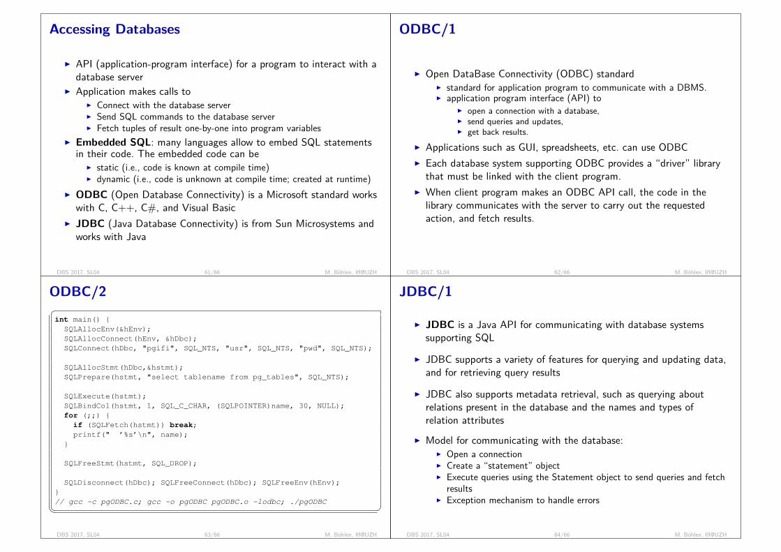
Accessing Databases
I API (application-program interface) for a program to interact with adatabase server
I Application makes calls toI Connect with the database serverI Send SQL commands to the database serverI Fetch tuples of result one-by-one into program variables
I Embedded SQL: many languages allow to embed SQL statementsin their code. The embedded code can be
I static (i.e., code is known at compile time)I dynamic (i.e., code is unknown at compile time; created at runtime)
I ODBC (Open Database Connectivity) is a Microsoft standard workswith C, C++, C#, and Visual Basic
I JDBC (Java Database Connectivity) is from Sun Microsystems andworks with Java
DBS 2017, SL04 61/66 M. Böhlen, IfI@UZH
ODBC/1
I Open DataBase Connectivity (ODBC) standardI standard for application program to communicate with a DBMS.I application program interface (API) to
I open a connection with a database,I send queries and updates,I get back results.
I Applications such as GUI, spreadsheets, etc. can use ODBCI Each database system supporting ODBC provides a “driver” library
that must be linked with the client program.I When client program makes an ODBC API call, the code in the
library communicates with the server to carry out the requestedaction, and fetch results.
DBS 2017, SL04 62/66 M. Böhlen, IfI@UZH
ODBC/2�int main() {
SQLAllocEnv(&hEnv);SQLAllocConnect(hEnv, &hDbc);SQLConnect(hDbc, "pgifi", SQL_NTS, "usr", SQL_NTS, "pwd", SQL_NTS);
SQLAllocStmt(hDbc,&hstmt);SQLPrepare(hstmt, "select tablename from pg_tables", SQL_NTS);
SQLExecute(hstmt);SQLBindCol(hstmt, 1, SQL_C_CHAR, (SQLPOINTER)name, 30, NULL);for (;;) {
if (SQLFetch(hstmt)) break;printf(" ’%s’\n", name);
}
SQLFreeStmt(hstmt, SQL_DROP);
SQLDisconnect(hDbc); SQLFreeConnect(hDbc); SQLFreeEnv(hEnv);}// gcc -c pgODBC.c; gcc -o pgODBC pgODBC.o -lodbc; ./pgODBC� �DBS 2017, SL04 63/66 M. Böhlen, IfI@UZH
JDBC/1
I JDBC is a Java API for communicating with database systemssupporting SQL
I JDBC supports a variety of features for querying and updating data,and for retrieving query results
I JDBC also supports metadata retrieval, such as querying aboutrelations present in the database and the names and types ofrelation attributes
I Model for communicating with the database:I Open a connectionI Create a “statement” objectI Execute queries using the Statement object to send queries and fetch
resultsI Exception mechanism to handle errors
DBS 2017, SL04 64/66 M. Böhlen, IfI@UZH

JDBC/2�import java.sql.*;
public class pgJDBC {public static void main(String[] argv) {
Class.forName("org.postgresql.Driver");
Connection conn = DriverManager.getConnection("jdbc:postgresql://pg.ifi.uzh.ch/boehlen?ssl=true" +"&sslfactory=org.postgresql.ssl.NonValidatingFactory","boehlen", "xxx");
Statement stmt = conn.createStatement();
ResultSet rset = stmt.executeQuery("select tablename from pg_tables where tableowner=’boehlen’");
while (rset.next())System.out.println(rset.getString(1));
}}// javac pgJDBC.java// java -classpath /usr/share/java/postgresql-jdbc4-9.2.jar:. pgJDBC� �DBS 2017, SL04 65/66 M. Böhlen, IfI@UZH
Summary
I Views are essential to break up large tasks (SQL statements) insmall, independent and manageable blocks.
I Recursive queries are used to compute ancestors, descendants,transitive closures, etc.
I Integrity constraints ensure a good data quality. Enforcingintegrity constraints is not easy: people try to work around.
I Functions and procedural constructs are used heavily by manyapplications. For example PostGIS uses functions heavily to addadvanced spatial functionality to PostgreSQL.
I Program access is through ODBC and JDBC. General-purposegraphical tools exist to interact with databases.
DBS 2017, SL04 66/66 M. Böhlen, IfI@UZH
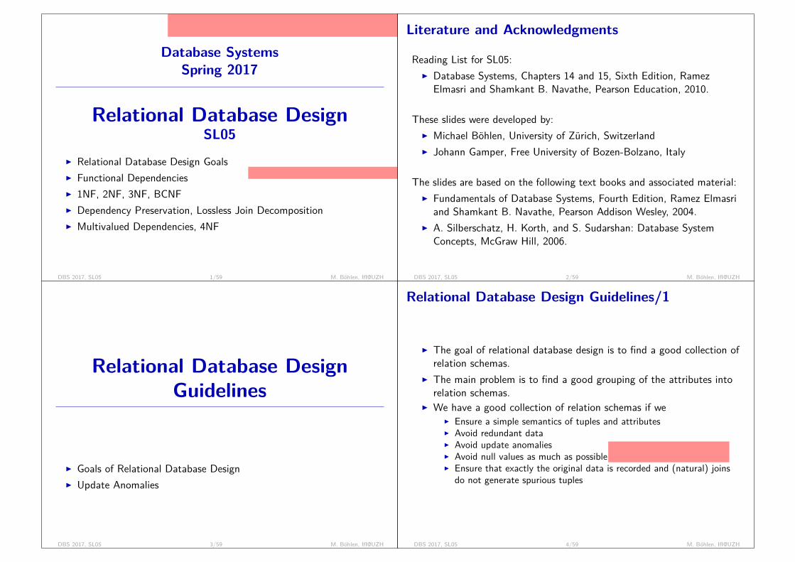
Database SystemsSpring 2017
Relational Database DesignSL05
I Relational Database Design GoalsI Functional DependenciesI 1NF, 2NF, 3NF, BCNFI Dependency Preservation, Lossless Join DecompositionI Multivalued Dependencies, 4NF
Reviews: 12 16 20 22 31 38 43 45 48 53
as a db designer it is important to understand pros and cons ofnormal forms (problems NFs create and solve)
DBS 2017, SL05 1/59 M. Böhlen, IfI@UZH
Literature and Acknowledgments
Reading List for SL05:I Database Systems, Chapters 14 and 15, Sixth Edition, Ramez
Elmasri and Shamkant B. Navathe, Pearson Education, 2010.
These slides were developed by:I Michael Böhlen, University of Zürich, SwitzerlandI Johann Gamper, Free University of Bozen-Bolzano, Italy
The slides are based on the following text books and associated material:I Fundamentals of Database Systems, Fourth Edition, Ramez Elmasri
and Shamkant B. Navathe, Pearson Addison Wesley, 2004.I A. Silberschatz, H. Korth, and S. Sudarshan: Database System
Concepts, McGraw Hill, 2006.
DBS 2017, SL05 2/59 M. Böhlen, IfI@UZH
Relational Database DesignGuidelines
I Goals of Relational Database DesignI Update Anomalies
DBS 2017, SL05 3/59 M. Böhlen, IfI@UZH
Relational Database Design Guidelines/1
I The goal of relational database design is to find a good collection ofrelation schemas.
I The main problem is to find a good grouping of the attributes intorelation schemas.
I We have a good collection of relation schemas if weI Ensure a simple semantics of tuples and attributesI Avoid redundant dataI Avoid update anomaliesI Avoid null values as much as possible
we get nulls if different things arecombined
I Ensure that exactly the original data is recorded and (natural) joinsdo not generate spurious tuples
DBS 2017, SL05 4/59 M. Böhlen, IfI@UZH

Relational Database Design Guidelines/2
I Consider the relation schema:I EmpProj(SSN, PNum, Hours, EName, PName, PLoc)
I Update Anomaly:I Changing the name of project location “Houston” to “Dallas” for an
employee forces us to make this change for all other employeesworking on this project.
if we want one location per project
I Insert Anomaly:I Cannot insert a project unless an employee is assigned to it (except
by using null values).
but: no null values allowed for PKs
I Delete Anomaly:I When a project is deleted, it will result in deleting all the employees
who work on that project.
DBS 2017, SL05 5/59 M. Böhlen, IfI@UZH
Relational Database Design Guidelines/3
SSN, PNum, Hours: no redundancyEName: redundancyPName, PLoc: redundancyintuition for redundancy: same inform stored multiple times
I Consider relation schemaEmpProj(SSN, PNum, Hours, EName, PName, Ploc)
with instanceempprojSSN PNum Hours EName PName PLoc1234 1 32.5 ’Smith’ ’ProductX’ ’Bellaire’1234 2 7.5 ’Smith’ ’ProductY’ ’Sugarland’6688 3 40.5 ’Narayan’ ’ProductZ’ ’Houston’4567 1 20.0 ’English’ ’ProductX’ ’Bellaire’4567 2 20.0 ’English’ ’ProductY’ ’Sugarland’3334 2 10.0 ’Wong’ ’ProductY’ ’Sugarland’3334 3 10.0 ’Wong’ ’ProductZ’ ’Houston’3334 10 10.0 ’Wong’ ’Computerization’ ’Stafford’3334 20 10.0 ’Wong’ ’Reorganization’ ’Houston’
I Relation schema EmpProj is not a good schema and suffers fromupdate anomalies.
DBS 2017, SL05 6/59 M. Böhlen, IfI@UZH
Relational Database Design Guidelines/4
I Guideline 1: Each tuple in a relation should only represent oneentity or relationship instance.
I Guideline 2: Design a schema that does not suffer from insertion,deletion and update anomalies.
I Guideline 3: Relations should be designed such that their tuples willhave as few NULL values as possible; attributes that are NULL shallbe placed in separate relations (along with the primary key).
I Guideline 4: Relations should be designed such that no spurious(i.e., wrong) tuples are generated if we do a natural join of therelations.
A B C1 3 62 3 2
6=A B1 32 3
1
B C3 63 2
=
A B C1 3 61 3 22 3 62 3 2
DBS 2017, SL05 7/59 M. Böhlen, IfI@UZH
Functional Dependencies
I DefinitionI Armstrong’s inference rulesI Soundness and completenessI Closure and minimal cover
DBS 2017, SL05 8/59 M. Böhlen, IfI@UZH

Keys (Refresher)
I A superkey of a relation schema R(A1,A2, . . . ,An) is a set ofattributes S ⊆ attr(R) with the property that no two tuples t1 andt2 in any legal relation state r of R will have t1[S] = t2[S]
I A candidate key K is a superkey with the additional property thatremoval of any attribute from K will cause the reduced K not to bea superkey any more.
I One of the candidate keys is arbitrarily chosen to be the primarykey.
I Notation: We underline the primary key attributes:EmpProj(SSN, PNum, Hours, EName, PName, Ploc)
Thus, (SSN,PNum) is a primary key of EmpProj
DBS 2017, SL05 9/59 M. Böhlen, IfI@UZH
Functional Dependencies/1
FDs generalize keys:I key determines all other attributesI FDs determine some other attributes
examples of trivial FDs:I SSN, LN -> LNI LN, FN -> FN
I Functional dependencies (FDs) are used to specify formal measuresof the goodness of relational designs.
I Functional dependencies and keys are used to define normal formsfor relations.
I Functional dependencies are constraints that are derived from themeaning and interrelationships of the attributes.
I A set of attributes X functionally determines a set of attributes Y ifthe value of X determines a unique value for Y.
SSN, SNumber , ...
I A functional dependency X → Y is trivial iff Y ⊆ X .
DBS 2017, SL05 10/59 M. Böhlen, IfI@UZH
Functional Dependencies/2
I X → Y denotes a functional dependency.I X → Y means that X functionally determines Y.I X → Y holds if whenever two tuples have the same value for X they
have the same value for Y.I For any two tuples t1 and t2 in any relation instance r(R) :
If t1[X ] = t2[X ] then t1[Y ] = t2[Y ]I X → Y for R specifies a constraint on the schema, i.e., on all
possible relation instances r(R).I FDs are derived from the real-world constraints on the attributes.
I Notation: instead of {A,B} we write AB (or A,B), e.g.,AB → BCD (instead of {A,B} → {B,C ,D})
DBS 2017, SL05 11/59 M. Böhlen, IfI@UZH
Review 5.1 rA B C1 1 32 1 13 2 24 1 1
Consider the relation instance r(R) and the statements1. A is a primary key of R2. B → C is a functional dependency that holds for R3. C → B is a functional dependency that holds for R4. BC → A is a functional dependency that relation instance r satisfies
Which of these statements are true?
1. possibly true2. false3. possibly true4. true
DBS 2017, SL05 12/59 M. Böhlen, IfI@UZH
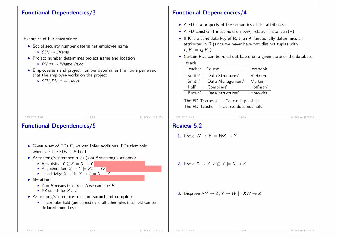
Functional Dependencies/3
Examples of FD constraints:I Social security number determines employee name
I SSN → ENameI Project number determines project name and location
I PNum→ PName,PLocI Employee ssn and project number determines the hours per week
that the employee works on the projectI SSN,PNum→ Hours
DBS 2017, SL05 13/59 M. Böhlen, IfI@UZH
Functional Dependencies/4
I A FD is a property of the semantics of the attributes.I A FD constraint must hold on every relation instance r(R)I If K is a candidate key of R, then K functionally determines all
attributes in R (since we never have two distinct tuples witht1[K ] = t2[K ])
I Certain FDs can be ruled out based on a given state of the database:teachTeacher Course Textbook’Smith’ ’Data Structures’ ’Bertram’’Smith’ ’Data Management’ ’Martin’’Hall’ ’Compilers’ ’Hoffman’’Brown’ ’Data Structures’ ’Horowitz’
The FD Textbook → Course is possibleThe FD Teacher → Course does not hold
DBS 2017, SL05 14/59 M. Böhlen, IfI@UZH
Functional Dependencies/5
I Given a set of FDs F , we can infer additional FDs that holdwhenever the FDs in F hold
I Armstrong’s inference rules (aka Armstrong’s axioms):I Reflexivity: Y ⊆ X |= X → Y
FN ⊆ FN, LN |= FN, LN → FN
I Augmentation: X → Y |= XZ → YZ
SSN → LN |= SSN, FN → LN, FN
I Transitivity: X → Y ,Y → Z |= X → Z
LN → Tlf , Tlf → Kt |= LN → Kt
I Notation:I A |= B means that from A we can infer BI XZ stands for X ∪ Z
I Armstrong’s inference rules are sound and completeI These rules hold (are correct) and all other rules that hold can be
deduced from these
DBS 2017, SL05 15/59 M. Böhlen, IfI@UZH
Review 5.21. Prove W → Y |= WX → Y
I WX → YX (augmentation)I YX → Y (reflexivity)I WX → Y (transitivity)
2. Prove X → Y ,Z ⊆ Y |= X → Z
I Y → Z (reflexivity)I X → Z (transitivity)
3. Disprove XY → Z ,Y →W |= XW → Z
X Y Z W1 1 1 11 2 2 1
DBS 2017, SL05 16/59 M. Böhlen, IfI@UZH

Functional Dependencies/6
I Additional inference rules that are useful:I Decomposition: X → YZ |= X → Y ,X → ZI Union: X → Y ,X → Z |= X → YZI Pseudotransitivity: X → Y ,WY → Z |= WX → Z
I The last three inference rules, as well as any other inference rules,can be deduced from Armstrong’s inference rules (because of thecompleteness property).
decomposition ex: SSN → FN, LN |= SSN → FN, SSN → LN
pseudotransitivity ex: LN → City , Kanton, City → PLZ |= LN, Kanton→ PLZ
DBS 2017, SL05 17/59 M. Böhlen, IfI@UZH
Functional Dependencies/7
I The closure of a set F of FDs is the set F + of all FDs that can beinferred from F .
I The closure of a set of attributes X with respect to F is the set X+
of all attributes that are functionally determined by X .I F + and X+ can be calculated by repeatedly applying Armstrong’s
inference rules to F and X , respectively.
DBS 2017, SL05 18/59 M. Böhlen, IfI@UZH
Functional Dependencies/8
I Two sets of FDs F and G are equivalent if:I Every FD in F can be inferred from G , andI Every FD in G can be inferred from FI Hence, F and G are equivalent if F + = G+
I Definition: F covers G if every FD in G can be inferred from F(i.e., if G+ ⊆ F +)
I F and G are equivalent if F covers G and G covers F
DBS 2017, SL05 19/59 M. Böhlen, IfI@UZH
Review 5.3Consider F = {A→ C ,AC → D,E → AD,E → H} andG = {A→ CD,E → AH}. Are F and G equivalent?
F:I A+ = ACDI AC+ = ACDI E+ = ACDEHI H+ = HI D+ = D
G:I A+ = ACDI AC+ = ACDI E+ = ACDEHI H+ = HI D+ = D
From F + = G+ we get F = G
DBS 2017, SL05 20/59 M. Böhlen, IfI@UZH
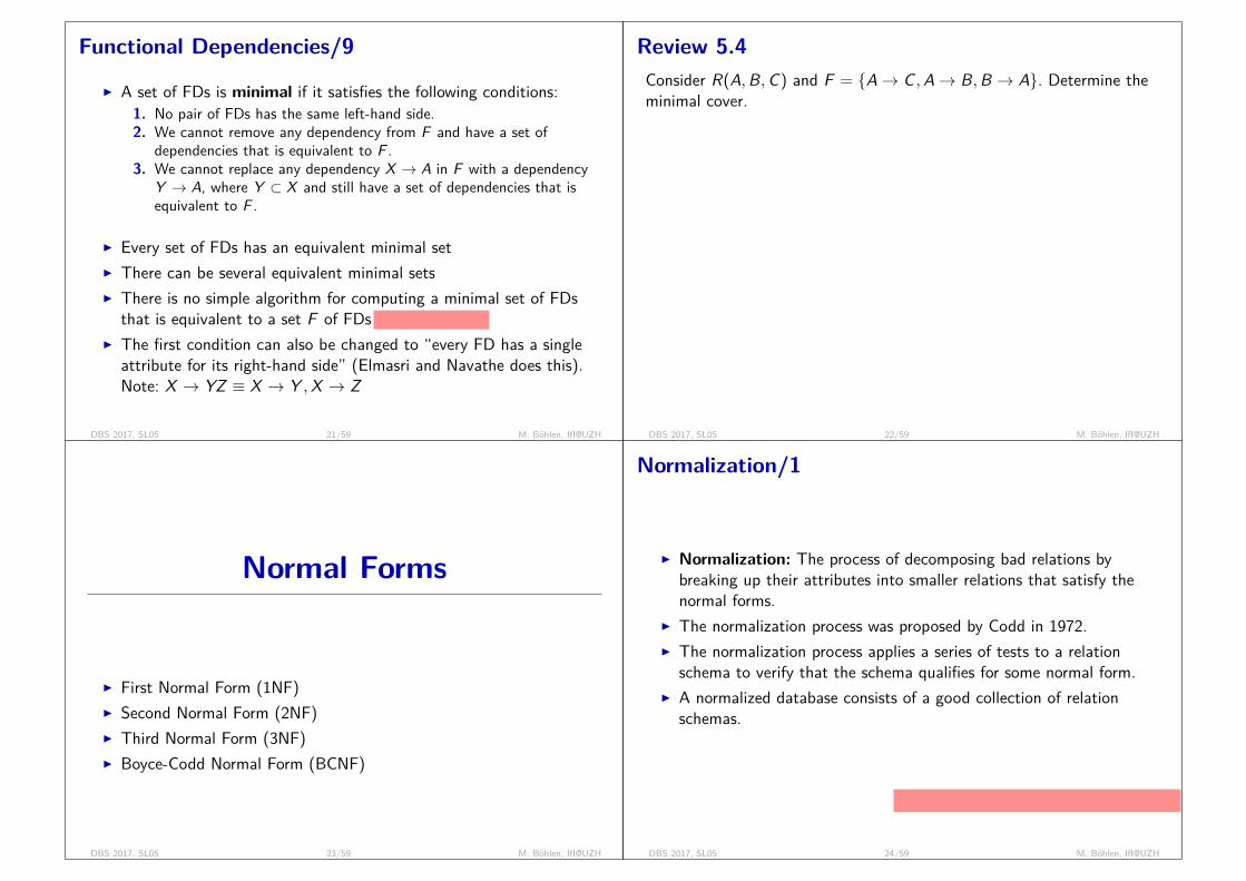
Functional Dependencies/9
I A set of FDs is minimal if it satisfies the following conditions:1. No pair of FDs has the same left-hand side.2. We cannot remove any dependency from F and have a set of
dependencies that is equivalent to F .3. We cannot replace any dependency X → A in F with a dependency
Y → A, where Y ⊂ X and still have a set of dependencies that isequivalent to F .
I Every set of FDs has an equivalent minimal setI There can be several equivalent minimal setsI There is no simple algorithm for computing a minimal set of FDs
that is equivalent to a set F of FDs
intuition is needed
I The first condition can also be changed to “every FD has a singleattribute for its right-hand side” (Elmasri and Navathe does this).Note: X → YZ ≡ X → Y ,X → Z
DBS 2017, SL05 21/59 M. Böhlen, IfI@UZH
Review 5.4Consider R(A,B,C) and F = {A→ C ,A→ B,B → A}. Determine theminimal cover.
I F + = {A→ ∗,B → ∗,C → C}I F +
min1 = {A→ BC ,B → A}I F +
min1 = {A→ B,B → AC}draw graphs
B??
��A
��C
B??
��
��
A
C
B??
��
��
A
��C
DBS 2017, SL05 22/59 M. Böhlen, IfI@UZH
Normal Forms
I First Normal Form (1NF)I Second Normal Form (2NF)I Third Normal Form (3NF)I Boyce-Codd Normal Form (BCNF)
DBS 2017, SL05 23/59 M. Böhlen, IfI@UZH
Normalization/1
I Normalization: The process of decomposing bad relations bybreaking up their attributes into smaller relations that satisfy thenormal forms.
I The normalization process was proposed by Codd in 1972.I The normalization process applies a series of tests to a relation
schema to verify that the schema qualifies for some normal form.I A normalized database consists of a good collection of relation
schemas.
data →(normalize) rdb →(denormalize) dw
DBS 2017, SL05 24/59 M. Böhlen, IfI@UZH

Normalization/2
I 1NFI attribute values must be atomic
I 2NF, 3NF, BCNFI based on candidate keys and FDs of a relation schema
I 4NFI based on candidate keys, multi-valued dependencies (MVDs)
I 5NFI based on candidate keys, join dependencies (JDs)
I Additional properties may be needed to ensure a good relationaldesign:
I Losslessness of the corresponding join (very important and cannot besacrificed)
I Preservation of the functional dependencies (less stringent and maybe sacrificed)
DBS 2017, SL05 25/59 M. Böhlen, IfI@UZH
Normalization/3
I In practice normalization is carried out to guarantee that theresulting schemas are of high quality
I The normalization process provides a deep understanding ofrelations and attributes.
I The database designers need not normalize to the highest possiblenormal form
I usually they choose 3NF, BCNF or 4NFI controlled redundancy is OK/good
I Denormalization:I The process of storing the join of higher normal form relations as a
base relation (which is in a lower normal form since the join destroysthe normal form)
DBS 2017, SL05 26/59 M. Böhlen, IfI@UZH
First Normal Form (1NF)/1
I DisallowsI composite attributesI multivalued attributesI nested relations: attributes whose values for an individual tuple are
relationsI Often 1NF is considered to be part of the definition of a relationI The following instance of schema
Department(DName,DNum,DMgrSSN,DLoc) is not in 1NF:departmentDName DNum DMgrSSN DLoc’Research’ 5 334455 {’Bellaire’, ’Sugarland’, ’Houston’ }’Administration’ 4 987654 { ’Stafford’ }’Headquarters’ 1 888666 { ’Houston’ }
DBS 2017, SL05 27/59 M. Böhlen, IfI@UZH
First Normal Form (1NF)/2
I Remedy to get 1NF: Form new relations for each multivaluedattribute or nested relation
I The following instance is the equivalent instance in 1NF:departmentDName DNum DMgrSSN DLoc’Research’ 5 334455 ’Bellaire’’Research’ 5 334455 ’Sugarland’’Research’ 5 334455 ’Houston’’Administration’ 4 987654 ’Stafford’’Headquarters’ 1 888666 ’Houston’
DBS 2017, SL05 28/59 M. Böhlen, IfI@UZH
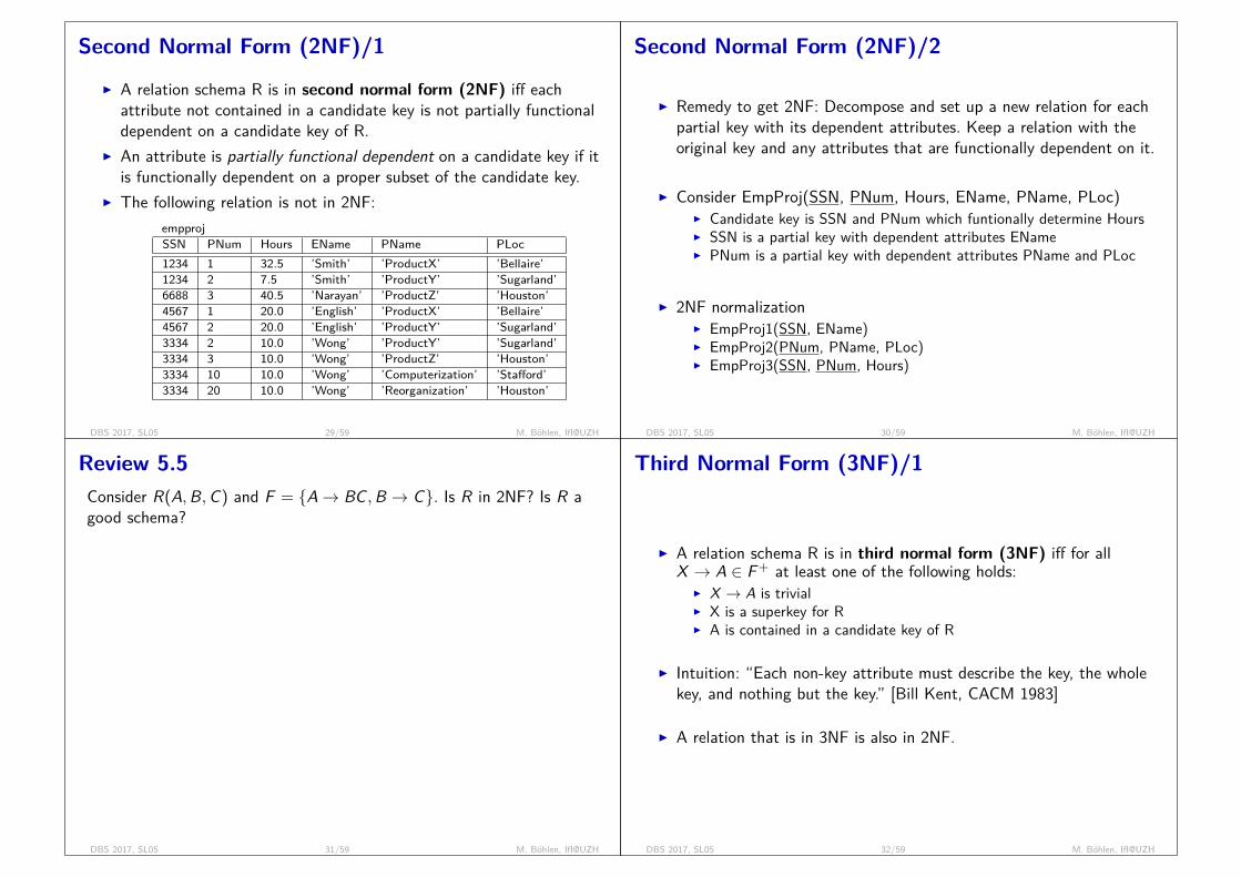
Second Normal Form (2NF)/1
I A relation schema R is in second normal form (2NF) iff eachattribute not contained in a candidate key is not partially functionaldependent on a candidate key of R.
I An attribute is partially functional dependent on a candidate key if itis functionally dependent on a proper subset of the candidate key.
I The following relation is not in 2NF:empprojSSN PNum Hours EName PName PLoc1234 1 32.5 ’Smith’ ’ProductX’ ’Bellaire’1234 2 7.5 ’Smith’ ’ProductY’ ’Sugarland’6688 3 40.5 ’Narayan’ ’ProductZ’ ’Houston’4567 1 20.0 ’English’ ’ProductX’ ’Bellaire’4567 2 20.0 ’English’ ’ProductY’ ’Sugarland’3334 2 10.0 ’Wong’ ’ProductY’ ’Sugarland’3334 3 10.0 ’Wong’ ’ProductZ’ ’Houston’3334 10 10.0 ’Wong’ ’Computerization’ ’Stafford’3334 20 10.0 ’Wong’ ’Reorganization’ ’Houston’
DBS 2017, SL05 29/59 M. Böhlen, IfI@UZH
Second Normal Form (2NF)/2
I Remedy to get 2NF: Decompose and set up a new relation for eachpartial key with its dependent attributes. Keep a relation with theoriginal key and any attributes that are functionally dependent on it.
I Consider EmpProj(SSN, PNum, Hours, EName, PName, PLoc)I Candidate key is SSN and PNum which funtionally determine HoursI SSN is a partial key with dependent attributes ENameI PNum is a partial key with dependent attributes PName and PLoc
I 2NF normalizationI EmpProj1(SSN, EName)I EmpProj2(PNum, PName, PLoc)I EmpProj3(SSN, PNum, Hours)
DBS 2017, SL05 30/59 M. Böhlen, IfI@UZH
Review 5.5Consider R(A,B,C) and F = {A→ BC ,B → C}. Is R in 2NF? Is R agood schema?
1. candidate key: Anon-candidate key: B, C; both depend fully on A
2. R is in 2NF (no non-candidate key attribute is partiallyfunctional dependent on a candidate key of R)
3. not a good (redundancy free) schemaA B C’a’ ’b’ ’c’’b’ ’b’ ’c’
SSN PhoneNr Kanton111 987 ’BE’222 987 ’BE’
DBS 2017, SL05 31/59 M. Böhlen, IfI@UZH
Third Normal Form (3NF)/1
I A relation schema R is in third normal form (3NF) iff for allX → A ∈ F + at least one of the following holds:
I X → A is trivialI X is a superkey for RI A is contained in a candidate key of R
I Intuition: “Each non-key attribute must describe the key, the wholekey, and nothing but the key.” [Bill Kent, CACM 1983]
I A relation that is in 3NF is also in 2NF.
DBS 2017, SL05 32/59 M. Böhlen, IfI@UZH

Third Normal Form (3NF)/2
I The following relation with the functional dependencies SC → Tand T → C is in 3NF:
rStudent Course Textbook’Smith’ ’Data Structures’ ’Bertram’’Smith’ ’Data Management’ ’Martin’’Hall’ ’Compilers’ ’Hoffman’’Brown’ ’Data Structures’ ’Horowitz’
I SC → T is OK since SC is a candidate key.I T → C is OK since C is contained in a candidate key.
I This relation is in 3NF but permits redundant information, whichcan lead to update anomalies.
DBS 2017, SL05 33/59 M. Böhlen, IfI@UZH
Third Normal Form (3NF)/3
I Consider adding a tuple to the above relation:rStudent Course Textbook’Smith’ ’Data Structures’ ’Bertram’’Smith’ ’Data Management’ ’Martin’’Hall’ ’Compilers’ ’Hoffman’’Brown’ ’Data Structures’ ’Horowitz’’Jones’ ’Data Structures’ ’Bertram’
I Assessment of solution:I Cons: The fact that Bertram is a textbook for the Data Structures
class is stored twiceI Pros: SC → T and T → C can be checked by looking at relation r
only (dependency preservation, will be discussed later)
DBS 2017, SL05 34/59 M. Böhlen, IfI@UZH
Boyce-Codd Normal Form (BCNF)/1
I A relation schema R is in Boyce-Codd Normal Form (BCNF) ifffor all X → A ∈ F + at least one of the following holds:
I X → A is trivialI X is a superkey for R
I Intuition: “Each attribute must describe the key, the whole key, andnothing but the key.” [Chris Date, adaption of Bill Kent for 3NF]
I A relation that is in BCNF is also in 3NF.
I There exist relations that are in 3NF but not in BCNF
DBS 2017, SL05 35/59 M. Böhlen, IfI@UZH
Boyce-Codd Normal Form (BCNF)/2
I The following relations with the functional dependencies SC → Tand T → C are in BCNF:r1Course Textbook’Data Structures’ ’Bertram’’Data Management’ ’Martin’’Compilers’ ’Hoffman’’Data Structures’ ’Horowitz’
r2Student Textbook’Smith’ ’Bertram’’Smith’ ’Martin’’Hall’ ’Hoffman’’Brown’ ’Horowitz’’Jones’ ’Horowitz’
I T → C is OK since T is a candidate key.I SC → T is not considered since it uses attributes from different
relations (a functional dependency is a constraint between two setsof attributes in a single relation).
DBS 2017, SL05 36/59 M. Böhlen, IfI@UZH

Boyce-Codd Normal Form (BCNF)/3
I With BCNF less redundancy exists but it is no longer possible tocheck all functional dependencies by looking at one relation only.
r1Course Textbook’Data Structures’ ’Bertram’’Data Management’ ’Martin’’Compilers’ ’Hoffman’’Data Structures’ ’Horowitz’
r2Student Textbook’’Smith’ ’Bertram’’Smith’ ’Martin’’Hall’ ’Hoffman’’Brown’ ’Horowitz’’Jones’ ’Horowitz’’Jones’ ’Bertram’
I Assessment of solution:I Pros: No information is stored redundantlyI Cons: The fact that Jones uses two textbooks for the Data Structures
class and therefore SC → T does not hold cannot be checkedwithout joining the relations
DBS 2017, SL05 37/59 M. Böhlen, IfI@UZH
Review 5.6Relation R satisfies BCNF:rA B C’a1’ ’b1’ ’c1’’a1’ ’b2’
Assume we know that the functional dependency A→ C holds. Whatvalue can we infer for the value that is missing?
I A→ C requires empty value to be c1
I BCNF requires A to be a key
I b1 6= b2 prevents A from being a key
I thus, impossible; r cannot be in BCNF
DBS 2017, SL05 38/59 M. Böhlen, IfI@UZH
Properties of Decompositionsand
Normalization Algorithm
I Dependency PreservationI Lossless Join DecompositionI BCNF Normalization Algorithm
DBS 2017, SL05 39/59 M. Böhlen, IfI@UZH
Multiple Relations
I Relational database design by decomposition:I Universal Relation Schema: A relation schema R(A1,A2, . . . ,An) that
includes all attributes of the database.I Decomposition: decompose the universal relation schema R into a set
of relation schemas D = R1,R2, . . . ,Rm by using the functionaldependencies.
I Additional conditions:I Each attribute in R will appear in at least one relation schema Ri in
the decomposition so that no attributes are lost.I Have each individual relation Ri in the decomposition D in 3NF (or
higher).I Lossless join decomposition: ensures that the decomposition does
not introduce wrong tuples when relations are joined together.I Dependency preservation: ensures that all functional dependency
can be checked by considering individual relations Ri only.
DBS 2017, SL05 40/59 M. Böhlen, IfI@UZH
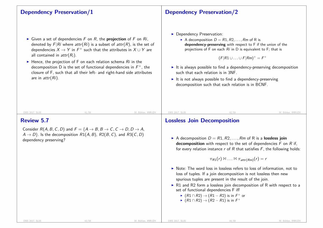
Dependency Preservation/1
I Given a set of dependencies F on R, the projection of F on Ri ,denoted by F |Ri where attr(Ri) is a subset of attr(R), is the set ofdependencies X → Y in F + such that the attributes in X ∪ Y areall contained in attr(Ri).
I Hence, the projection of F on each relation schema Ri in thedecomposition D is the set of functional dependencies in F +, theclosure of F, such that all their left- and right-hand side attributesare in attr(Ri).
DBS 2017, SL05 41/59 M. Böhlen, IfI@UZH
Dependency Preservation/2
I Dependency Preservation:I A decomposition D = R1,R2, . . . ,Rm of R isdependency-preserving with respect to F if the union of theprojections of F on each Ri in D is equivalent to F; that is
(F |R1 ∪ . . . ∪ F |Rm)+ = F +
I It is always possible to find a dependency-preserving decompositionsuch that each relation is in 3NF.
I It is not always possible to find a dependency-preservingdecomposition such that each relation is in BCNF.
DBS 2017, SL05 42/59 M. Böhlen, IfI@UZH
Review 5.7Consider R(A,B,C ,D) and F = {A→ B,B → C ,C → D,D → A,A→ D}. Is the decomposition R1(A,B), R2(B,C), and R3(C ,D)dependency preserving?
I F + = {A→ ∗,B → ∗,C → ∗,D → ∗}
I G = {A→ B,B → A,B → C ,C → B,C → D,D → C}
I G+ = {A→ ∗,B → ∗,C → ∗,D → ∗}
I thus, dependency preserving (F + = G+)
DBS 2017, SL05 43/59 M. Böhlen, IfI@UZH
Lossless Join Decomposition
I A decomposition D = R1,R2, . . . ,Rm of R is a lossless joindecomposition with respect to the set of dependencies F on R if,for every relation instance r of R that satisfies F , the following holds:
πR1(r) 1 . . . 1 πattr(Rm)(r) = r
I Note: The word loss in lossless refers to loss of information, not toloss of tuples. If a join decomposition is not lossless then newspurious tuples are present in the result of the join.
I R1 and R2 form a lossless join decomposition of R with respect to aset of functional dependencies F iff
I (R1 ∩ R2)→ (R1− R2) is in F + orI (R1 ∩ R2)→ (R2− R1) is in F +
DBS 2017, SL05 44/59 M. Böhlen, IfI@UZH
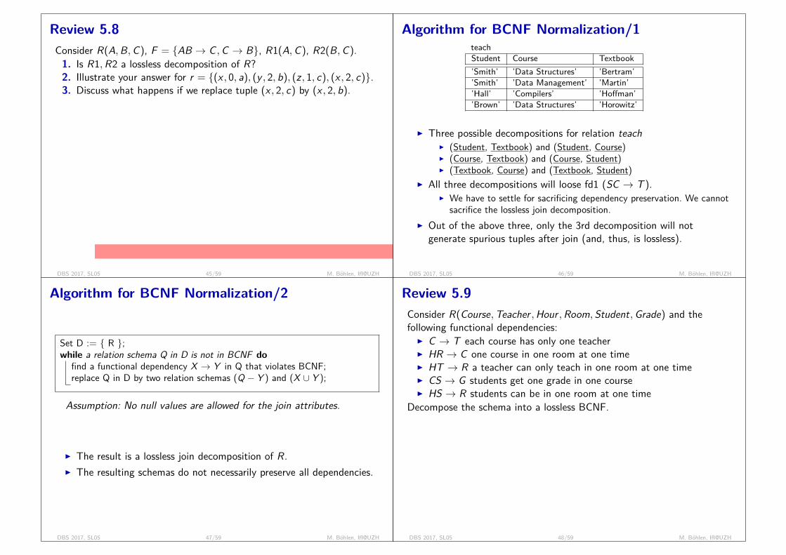
Review 5.8Consider R(A,B,C), F = {AB → C ,C → B}, R1(A,C), R2(B,C).1. Is R1,R2 a lossless decomposition of R?2. Illustrate your answer for r = {(x , 0, a), (y , 2, b), (z , 1, c), (x , 2, c)}.3. Discuss what happens if we replace tuple (x , 2, c) by (x , 2, b).
A B Cx 0 ay 2 bz 1 cx 2 c
6=
A Cx ay bz cx c
1
B C0 a2 b1 c2 c
=
A B Cx 0 ay 2 bz 1 cz 2 cx 2 cx 1 c
lossy decomposition;C → B 6∈ F +
A B Cx 0 ay 2 bz 1 cx 2 b
=
A Cx ay bz cx b
1
B C0 a2 b1 c
=
A B Cx 0 ay 2 bz 1 cx 2 b
lossless decomposition;C → B ∈ F +
R1 ∩ R2 = AC ∩ BC = C , R1− R2 = A, R2− R1 = B, C → A 6∈ F +, C → B ∈ F +
DBS 2017, SL05 45/59 M. Böhlen, IfI@UZH
Algorithm for BCNF Normalization/1teachStudent Course Textbook’Smith’ ’Data Structures’ ’Bertram’’Smith’ ’Data Management’ ’Martin’’Hall’ ’Compilers’ ’Hoffman’’Brown’ ’Data Structures’ ’Horowitz’
I Three possible decompositions for relation teachI (Student, Textbook) and (Student, Course)I (Course, Textbook) and (Course, Student)I (Textbook, Course) and (Textbook, Student)
I All three decompositions will loose fd1 (SC → T ).I We have to settle for sacrificing dependency preservation. We cannot
sacrifice the lossless join decomposition.I Out of the above three, only the 3rd decomposition will not
generate spurious tuples after join (and, thus, is lossless).
DBS 2017, SL05 46/59 M. Böhlen, IfI@UZH
Algorithm for BCNF Normalization/2
Set D := { R };while a relation schema Q in D is not in BCNF do
find a functional dependency X → Y in Q that violates BCNF;replace Q in D by two relation schemas (Q − Y ) and (X ∪ Y );
Assumption: No null values are allowed for the join attributes.
I The result is a lossless join decomposition of R.I The resulting schemas do not necessarily preserve all dependencies.
DBS 2017, SL05 47/59 M. Böhlen, IfI@UZH
Review 5.9Consider R(Course,Teacher ,Hour ,Room, Student,Grade) and thefollowing functional dependencies:I C → T each course has only one teacherI HR → C one course in one room at one timeI HT → R a teacher can only teach in one room at one timeI CS → G students get one grade in one courseI HS → R students can be in one room at one time
Decompose the schema into a lossless BCNF.
C → T : R1(CHRSG), R2(CT)HR → C : R3(HRSG), R2(CT) R4(HRC)HS is candidate key: HS, RHS, RHSC, RHSCT, RHSCTG
HS → R: Ra(CTHSG), Rb(HSR)C → T : Rc(CHSG) Rb(HSR) Rd(CT)CS → G: Re(CHS) Rb(HSR) Rd(CT) Rf(CSG)
CS → G: Ra(CTHSR) Rb(CSG)HT → R: Rc(CTHS) Rb(CSG) Rd(HTR)C → T : Re(CHS) Rb(CSG) Rd(HTR) Rf(CT)
DBS 2017, SL05 48/59 M. Böhlen, IfI@UZH

Discussion of BCNF Normalization
I It is valuable to construct a good schema that is in BCNF.I The normalization process gives important insights into the
properties of the data.I A potential difficulty is that the database designer must first specify
all the relevant functional dependencies among the databaseattributes.
I The normalization algorithms are not deterministic in general (e.g.,not a unique minimal cover).
I It is not always possible to find a decomposition into relationschemas that preserves dependencies and allows each relationschema in the decomposition to be in BCNF.
DBS 2017, SL05 49/59 M. Böhlen, IfI@UZH
3NF versus BCNF
I It is possible to construct a decomposition that is in BCNF and islossless
I It is possible to construct a decomposition that is in 3NF, is lossless,and preserves dependency.
I It is not always possible to construct a decomposition that is inBCNF, is lossless, and is dependency preserving.
I 3NF allows redundancies that BCNF does not allow.I BCNF cannot check all functional dependencies efficiently since
multiple relations must be considered for the check.I The application needs to determine if a BCNF or 3NF
decomposition should be chosen.
DBS 2017, SL05 50/59 M. Böhlen, IfI@UZH
Multivalued Dependencies
I DefinitionI Fourth Normal Form (4NF)
DBS 2017, SL05 51/59 M. Böhlen, IfI@UZH
Multivalued Dependencies/1
Definition:I A multivalued dependency (MVD) X � Y on relation schema R,
where X and Y are both subsets of R, specifies the followingconstraint on any relation instance r of R:If two tuples t1 and t2 exist in r such that t1[X ] = t2[X ], then twotuples t3 and t4 should also exist in r with the following properties,where we use Z to denote (R − (X ∪ Y )):
I t3[X ] = t4[X ] = t1[X ] = t2[X ].I t3[Y ] = t1[Y ] and t4[Y ] = t2[Y ].I t3[Z ] = t2[Z ] and t4[Z ] = t1[Z ].
I A MVD X � Y for R is called a trivial MVD if Y ⊂ X orX ∪ Y = attr(R).
DBS 2017, SL05 52/59 M. Böhlen, IfI@UZH
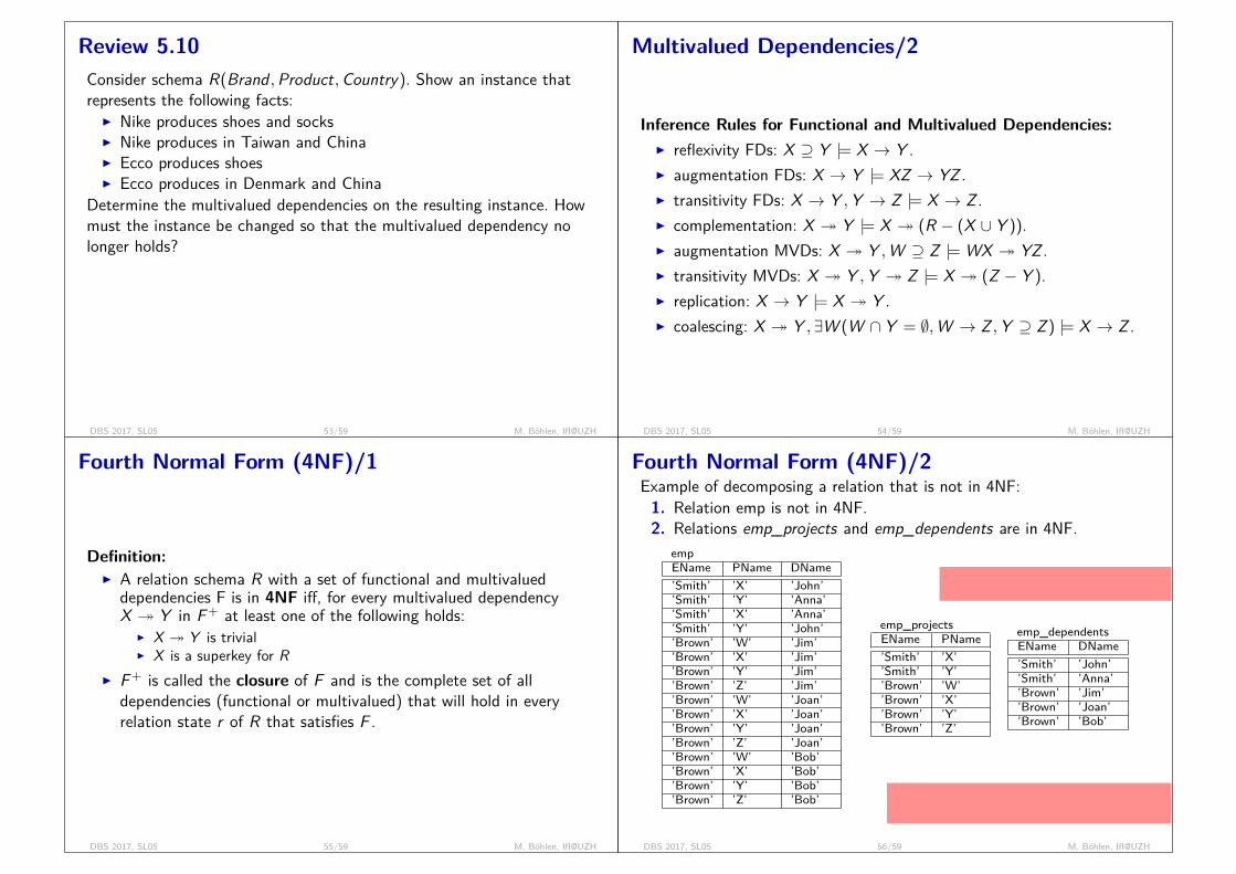
Review 5.10Consider schema R(Brand ,Product,Country). Show an instance thatrepresents the following facts:I Nike produces shoes and socksI Nike produces in Taiwan and ChinaI Ecco produces shoesI Ecco produces in Denmark and China
Determine the multivalued dependencies on the resulting instance. Howmust the instance be changed so that the multivalued dependency nolonger holds?
Brand Prod Ctry’Nike’ ’shoes’ ’Italy’’Nike’ ’socks’ ’Italy’’Nike’ ’shoes’ ’China’’Nike’ ’socks’ ’China’’Ecco’ ’shoes’ ’DK’’Ecco’ ’shoes’ ’China’
≡Brand Prod Ctry’Nike’ { ’shoes’, ’socks’ } { ’Italy’, ’China’ }’Ecco’ { ’shoes’ } { ’DK’, ’China’ }
DBS 2017, SL05 53/59 M. Böhlen, IfI@UZH
Multivalued Dependencies/2
Inference Rules for Functional and Multivalued Dependencies:I reflexivity FDs: X ⊇ Y |= X → Y .I augmentation FDs: X → Y |= XZ → YZ .I transitivity FDs: X → Y ,Y → Z |= X → Z .I complementation: X � Y |= X � (R − (X ∪ Y )).I augmentation MVDs: X � Y ,W ⊇ Z |= WX � YZ .I transitivity MVDs: X � Y ,Y � Z |= X � (Z − Y ).I replication: X → Y |= X � Y .I coalescing: X � Y , ∃W (W ∩ Y = ∅,W → Z ,Y ⊇ Z ) |= X → Z .
DBS 2017, SL05 54/59 M. Böhlen, IfI@UZH
Fourth Normal Form (4NF)/1
Definition:I A relation schema R with a set of functional and multivalued
dependencies F is in 4NF iff, for every multivalued dependencyX � Y in F + at least one of the following holds:
I X � Y is trivialI X is a superkey for R
I F + is called the closure of F and is the complete set of alldependencies (functional or multivalued) that will hold in everyrelation state r of R that satisfies F .
DBS 2017, SL05 55/59 M. Böhlen, IfI@UZH
Fourth Normal Form (4NF)/2Example of decomposing a relation that is not in 4NF:1. Relation emp is not in 4NF.2. Relations emp_projects and emp_dependents are in 4NF.
empEName PName DName’Smith’ ’X’ ’John’’Smith’ ’Y’ ’Anna’’Smith’ ’X’ ’Anna’’Smith’ ’Y’ ’John’’Brown’ ’W’ ’Jim’’Brown’ ’X’ ’Jim’’Brown’ ’Y’ ’Jim’’Brown’ ’Z’ ’Jim’’Brown’ ’W’ ’Joan’’Brown’ ’X’ ’Joan’’Brown’ ’Y’ ’Joan’’Brown’ ’Z’ ’Joan’’Brown’ ’W’ ’Bob’’Brown’ ’X’ ’Bob’’Brown’ ’Y’ ’Bob’’Brown’ ’Z’ ’Bob’
emp_projectsEName PName’Smith’ ’X’’Smith’ ’Y’’Brown’ ’W’’Brown’ ’X’’Brown’ ’Y’’Brown’ ’Z’
emp_dependentsEName DName’Smith’ ’John’’Smith’ ’Anna’’Brown’ ’Jim’’Brown’ ’Joan’’Brown’ ’Bob’
are MVDs possible? count as a check: 4= 2*2 or 4*1; 12 = 4*3 or ...
Smith { X, Y} { John, Anna }Brown {X, Y, W, Z} { Jim, Jean, Bob }
DBS 2017, SL05 56/59 M. Böhlen, IfI@UZH
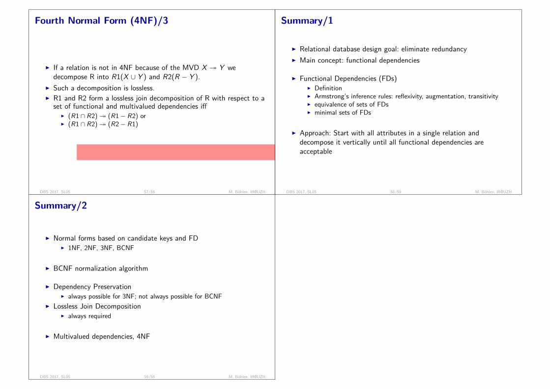
Fourth Normal Form (4NF)/3
I If a relation is not in 4NF because of the MVD X � Y wedecompose R into R1(X ∪ Y ) and R2(R − Y ).
I Such a decomposition is lossless.I R1 and R2 form a lossless join decomposition of R with respect to a
set of functional and multivalued dependencies iffI (R1 ∩ R2)� (R1− R2) orI (R1 ∩ R2)� (R2− R1)
last conditions ensure that from common attributes all the other attributes of arelation can be derived (the common attributes are a key of one relation)
DBS 2017, SL05 57/59 M. Böhlen, IfI@UZH
Summary/1
I Relational database design goal: eliminate redundancyI Main concept: functional dependencies
I Functional Dependencies (FDs)I DefinitionI Armstrong’s inference rules: reflexivity, augmentation, transitivityI equivalence of sets of FDsI minimal sets of FDs
I Approach: Start with all attributes in a single relation anddecompose it vertically until all functional dependencies areacceptable
DBS 2017, SL05 58/59 M. Böhlen, IfI@UZH
Summary/2
I Normal forms based on candidate keys and FDI 1NF, 2NF, 3NF, BCNF
I BCNF normalization algorithm
I Dependency PreservationI always possible for 3NF; not always possible for BCNF
I Lossless Join DecompositionI always required
I Multivalued dependencies, 4NF
DBS 2017, SL05 59/59 M. Böhlen, IfI@UZH
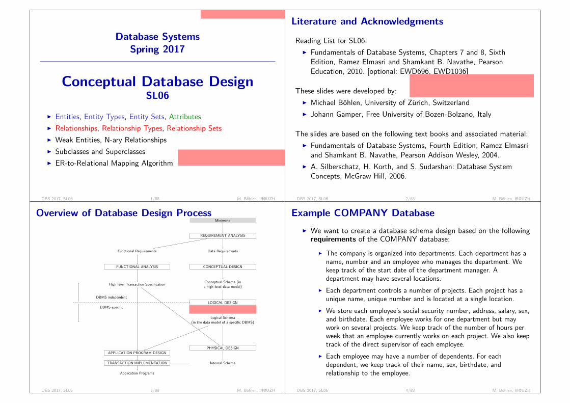
Database SystemsSpring 2017
Conceptual Database DesignSL06
I Entities, Entity Types, Entity Sets, AttributesI Relationships, Relationship Types, Relationship SetsI Weak Entities, N-ary RelationshipsI Subclasses and SuperclassesI ER-to-Relational Mapping Algorithm
Reviews: 11 31 37 38 56 66 75
UML: programs, behaviorER: data, modeling of a static mini world
DBS 2017, SL06 1/88 M. Böhlen, IfI@UZH
Literature and Acknowledgments
Reading List for SL06:I Fundamentals of Database Systems, Chapters 7 and 8, Sixth
Edition, Ramez Elmasri and Shamkant B. Navathe, PearsonEducation, 2010. [optional: EWD696, EWD1036]
Edsgar W. Dijkstra; streitbarer Mathematiker/Informatiker; problem of graphical notation: noprecise definition of correct/wrong
These slides were developed by:I Michael Böhlen, University of Zürich, SwitzerlandI Johann Gamper, Free University of Bozen-Bolzano, Italy
The slides are based on the following text books and associated material:I Fundamentals of Database Systems, Fourth Edition, Ramez Elmasri
and Shamkant B. Navathe, Pearson Addison Wesley, 2004.I A. Silberschatz, H. Korth, and S. Sudarshan: Database System
Concepts, McGraw Hill, 2006.
DBS 2017, SL06 2/88 M. Böhlen, IfI@UZH
Overview of Database Design Process
REQUIREMENT ANALYSIS
Data Requirements
Miniworld
Functional Requirements
CONCEPTUAL DESIGNFUNCTIONAL ANALYSIS
Conceptual Schema (ina high level data model)High level Transaction Specification
LOGICAL DESIGN
Logical Schema(in the data model of a specific DBMS)
PHYSICAL DESIGN
Internal SchemaTRANSACTION IMPLEMENTATION
Application Programs
APPLICATION PROGRAM DESIGN
DBMS independent
DBMS specific
relational model, RA, RC, SQL
DBS 2017, SL06 3/88 M. Böhlen, IfI@UZH
Example COMPANY DatabaseI We want to create a database schema design based on the followingrequirements of the COMPANY database:
I The company is organized into departments. Each department has aname, number and an employee who manages the department. Wekeep track of the start date of the department manager. Adepartment may have several locations.
I Each department controls a number of projects. Each project has aunique name, unique number and is located at a single location.
I We store each employee’s social security number, address, salary, sex,and birthdate. Each employee works for one department but maywork on several projects. We keep track of the number of hours perweek that an employee currently works on each project. We also keeptrack of the direct supervisor of each employee.
I Each employee may have a number of dependents. For eachdependent, we keep track of their name, sex, birthdate, andrelationship to the employee.
DBS 2017, SL06 4/88 M. Böhlen, IfI@UZH

Entities and Attributes
I Entities, entity types, entity setsI Attributes
DBS 2017, SL06 5/88 M. Böhlen, IfI@UZH
Entities and AttributesI Entities are specific objects or things in the mini-world that are
represented in the database.I For example employee John Smith, the Research department, project
ProductXI Attributes are properties used to describe an entity.
I For example an employee entity may have the attributes Name, SSN,Address, Sex, BirthDate
I A specific entity will have a value for each of its attributes.I For example a specific employee entity may have
Name = ’John Smith’,SSN = ’123456789’,Address = ’731, Fondren, Houston, TX’,Sex = ’M’,BirthDate = ’09-JAN-55‘
I Each attribute has a domain (value set, data type) associated withit, e.g., enumerated type, integer, string, subrange, . . .
DBS 2017, SL06 6/88 M. Böhlen, IfI@UZH
Types of Attributes/1
I Simple attributeI Each entity has a single atomic value for the attribute. For example,
SSN or Sex.I Composite attribute
I The attribute may be composed of several components. For example:I Address(Apt#, House#, Street, City, State, ZipCode, Country), orI Name(FirstName, MiddleName, LastName).
I Multi-valued attributeI An entity may have multiple values for that attribute. For example,
colors of a car or degrees of a student.I Denoted as {Color} or {PreviousDegree}.
I Derived attributeI Attributes can be derived (computed) rather than stored. Attribute
NumEmployees is a derived attribute.
DBS 2017, SL06 7/88 M. Böhlen, IfI@UZH
Types of Attributes/2
I Composite and multi-valued attributes may be nested arbitrarily toany number of levels.
I For example, PreviousDegree of a student is a compositemulti-valued attribute denoted by{PreviousDegree(College, Year, Degree, Field)}
I Multiple PreviousDegree values can existI Each has four subcomponent attributes:
I College, Year, Degree, FieldI A hierarchy of composite attributes:
Address
StreetAddress City State Zip
Number Street ApartmentNumber
DBS 2017, SL06 8/88 M. Böhlen, IfI@UZH
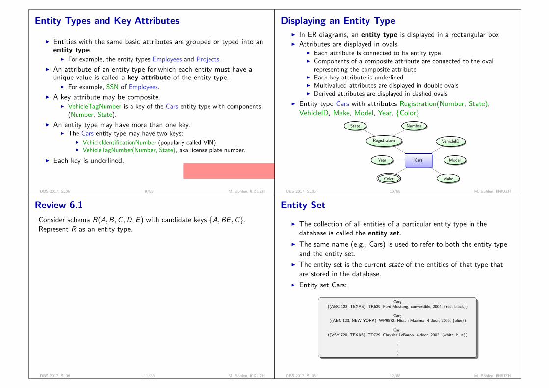
Entity Types and Key Attributes
I Entities with the same basic attributes are grouped or typed into anentity type.
I For example, the entity types Employees and Projects.I An attribute of an entity type for which each entity must have a
unique value is called a key attribute of the entity type.I For example, SSN of Employees.
I A key attribute may be composite.I VehicleTagNumber is a key of the Cars entity type with components
(Number, State).I An entity type may have more than one key.
I The Cars entity type may have two keys:I VehicleIdentificationNumber (popularly called VIN)I VehicleTagNumber(Number, State), aka license plate number.
I Each key is underlined.
VTagN: NummernschildVIdentificationN: Fahrzeugnummer
DBS 2017, SL06 9/88 M. Böhlen, IfI@UZH
Displaying an Entity TypeI In ER diagrams, an entity type is displayed in a rectangular boxI Attributes are displayed in ovals
I Each attribute is connected to its entity typeI Components of a composite attribute are connected to the oval
representing the composite attributeI Each key attribute is underlinedI Multivalued attributes are displayed in double ovalsI Derived attributes are displayed in dashed ovals
I Entity type Cars with attributes Registration(Number, State),VehicleID, Make, Model, Year, {Color}
CarsYear Model
Color Make
Registration VehicleID
NumberState
DBS 2017, SL06 10/88 M. Böhlen, IfI@UZH
Review 6.1Consider schema R(A,B,C ,D,E ) with candidate keys {A,BE ,C}.Represent R as an entity type.
RA
C
D
X
E B
DBS 2017, SL06 11/88 M. Böhlen, IfI@UZH
Entity SetI The collection of all entities of a particular entity type in the
database is called the entity set.I The same name (e.g., Cars) is used to refer to both the entity type
and the entity set.I The entity set is the current state of the entities of that type that
are stored in the database.I Entity set Cars:
Car1((ABC 123, TEXAS), TK629, Ford Mustang, convertible, 2004, {red, black})
Car2((ABC 123, NEW YORK), WP9872, Nissan Maxima, 4-door, 2005, {blue})
Car3((VSY 720, TEXAS), TD729, Chrysler LeBaron, 4-door, 2002, {white, blue})
.
.
.
DBS 2017, SL06 12/88 M. Böhlen, IfI@UZH

Entity Types for the COMPANY Database/1
I Based on the requirements, we can identify four initial entity typesin the COMPANY database:
I DepartmentsI ProjectsI EmployeesI Dependents
I The initial attributes are derived from the requirements descriptionI Guidelines for determining entity types and attributes:
I The nouns in a descriptions translate to entity typesI “organized into departments”
I Nouns that describe nouns of entity types translate to attributesI “department has a name, number”
Address? attribute or entity?attribute if address is mainly a property of employees;entity if application is managing addresses as independent object
DBS 2017, SL06 13/88 M. Böhlen, IfI@UZH
Entity Types for the COMPANY Database/2
Employees
SSN
BirthDate Name
FirstName LastName
Address Salary
Sex
Departments
Projects
Manager
Departments
NameLocations
Nummer
NumEmployees
Manager
ManagerStartDate
Projects
Name NummerLocation
ControllingInstitute
Dependents
Name Sex BDate Beziehung
Employee
derivedmulti-valuedkey
e.g., children;key? none.
because of space attributes are often omitted inthe graphical notation
DBS 2017, SL06 14/88 M. Böhlen, IfI@UZH
Relationships
I Relationships, Relationship Types, Relationship SetsI Structural Constraints on RelationshipsI Recursive RelationshipsI Attributes of Relationships
DBS 2017, SL06 15/88 M. Böhlen, IfI@UZH
Relationships and Relationship Types/1
I ER model has three main concepts:I Entities (and their entity types and entity sets)I Attributes (simple, composite, multivalued)I Relationships (and their relationship types and relationship sets)
I The initial design is typically not complete.I The schema design process is an iterative refinement process.
The initial design is created and iteratively refined.I Some aspects in the requirements will be represented asrelationships.
DBS 2017, SL06 16/88 M. Böhlen, IfI@UZH
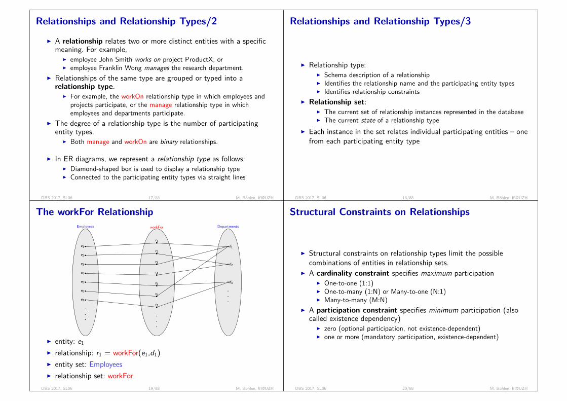
Relationships and Relationship Types/2
I A relationship relates two or more distinct entities with a specificmeaning. For example,
I employee John Smith works on project ProductX, orI employee Franklin Wong manages the research department.
I Relationships of the same type are grouped or typed into arelationship type.
I For example, the workOn relationship type in which employees andprojects participate, or the manage relationship type in whichemployees and departments participate.
I The degree of a relationship type is the number of participatingentity types.
I Both manage and workOn are binary relationships.
I In ER diagrams, we represent a relationship type as follows:I Diamond-shaped box is used to display a relationship typeI Connected to the participating entity types via straight lines
DBS 2017, SL06 17/88 M. Böhlen, IfI@UZH
Relationships and Relationship Types/3
I Relationship type:I Schema description of a relationshipI Identifies the relationship name and the participating entity typesI Identifies relationship constraints
I Relationship set:I The current set of relationship instances represented in the databaseI The current state of a relationship type
I Each instance in the set relates individual participating entities – onefrom each participating entity type
DBS 2017, SL06 18/88 M. Böhlen, IfI@UZH
The workFor RelationshipEmployees workFor Departments
e1
e2
e3
e4
e5
e6
e7
r1
r2
r3
r4
r5
r6
r7
d1
d2
d3
... ...
...
I entity: e1I relationship: r1 = workFor(e1,d1)I entity set: EmployeesI relationship set: workFor
DBS 2017, SL06 19/88 M. Böhlen, IfI@UZH
Structural Constraints on Relationships
I Structural constraints on relationship types limit the possiblecombinations of entities in relationship sets.
I A cardinality constraint specifies maximum participationI One-to-one (1:1)I One-to-many (1:N) or Many-to-one (N:1)I Many-to-many (M:N)
I A participation constraint specifies minimum participation (alsocalled existence dependency)
I zero (optional participation, not existence-dependent)I one or more (mandatory participation, existence-dependent)
DBS 2017, SL06 20/88 M. Böhlen, IfI@UZH
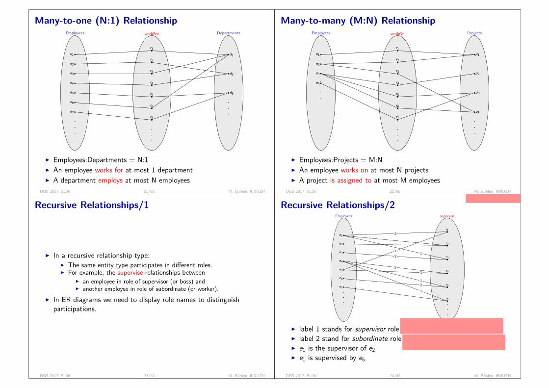
Many-to-one (N:1) RelationshipEmployees workFor Departments
e1
e2
e3
e4
e5
e6
e7
r1
r2
r3
r4
r5
r6
r7
d1
d2
d3
... ...
...
I Employees:Departments = N:1I An employee works for at most 1 departmentI A department employs at most N employees
DBS 2017, SL06 21/88 M. Böhlen, IfI@UZH
Many-to-many (M:N) RelationshipEmployees workOn Projects
e1
e2
e3
e4
r1
r2
r3
r4
r5
r6
r7
p1
p2
p3
p4
..
.
...
...
I Employees:Projects = M:NI An employee works on at most N projectsI A project is assigned to at most M employees
DBS 2017, SL06 22/88 M. Böhlen, IfI@UZH
Recursive Relationships/1
I In a recursive relationship type:I The same entity type participates in different roles.I For example, the supervise relationships between
I an employee in role of supervisor (or boss) andI another employee in role of subordinate (or worker).
I In ER diagrams we need to display role names to distinguishparticipations.
DBS 2017, SL06 23/88 M. Böhlen, IfI@UZH
Recursive Relationships/2Employees supervise
e1
e2
e3
e4
e5
e6
e7
r1
r2
r3
r4
r5
r6
21
1
2
2
2
1
1
1
1
2
2... ...
I label 1 stands for supervisor role
for each emp an number of edges with a1 (subordinate; Unterstellter)
I label 2 stand for subordinate role
for each emp at most one edge with a 2(boss)
I e1 is the supervisor of e2I e1 is supervised by e5
e5;e1,e4;e2,e3,e6,e7
DBS 2017, SL06 24/88 M. Böhlen, IfI@UZH

Attributes of Relationship Types
I A relationship type can have attributes:I For example, HoursPerWeek of workOnI Its value for each relationship instance describes the number of hours
per week that an employee works on a project.I A value of HoursPerWeek depends on a particular (employee, project)
combinationI Most relationship attributes are used with M:N relationships
I In 1:N relationships, they can be transferred to the entity type on theN-side of the relationship
DBS 2017, SL06 25/88 M. Böhlen, IfI@UZH
Notation for Constraints on Relationships/1
I Cardinality constraints (of a binary relationship): 1:1, 1:N, N:1, orM:N
I Cardinality constraints are shown by placing appropriate numbers onthe relationship edges.
Employees manage1
Departments1
I Reading is from left-to-right and top-down (usually; there are alwaysexceptions) and the terms are chosen accordingly.
I Reading: An employee manages 1 departmentI Inverse: A department is managed by 1 employee
leitet
DBS 2017, SL06 26/88 M. Böhlen, IfI@UZH
Notation for Constraints on Relationships/2
I Participation constraint on each participating entity type:total (called existence dependency) or partial.
I Total participation is shown by double line, partial participation bysingle line.
Employees workForN
Departments1
I A total participation constraint specifies a minimum participation:I An employee must workFor a departmentI A department must giveWorkTo N employees
I Structural constraints are easy to specify for binary relationshiptypes but get more subtle for higher order relationship types.
DBS 2017, SL06 27/88 M. Böhlen, IfI@UZH
Relationships for the COMPANY Database/1
I By examining the requirements, six relationship types are identifiedI All are binary relationships (degree 2)I Relationship types with participating entity types:
I workFor (between Employees and Departments)I manage (also between Employees and Departments)
leiten
I control (between Departments and Projects)I workOn (between Employees and Projects)I supervise (between Employees (as subordinate) and Employees (as
supervisor))
führen
I dependentsOf (between Employees and Dependents)
DBS 2017, SL06 28/88 M. Böhlen, IfI@UZH
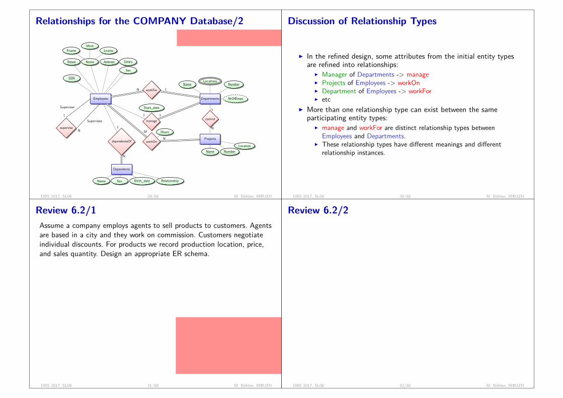
Relationships for the COMPANY Database/2
reading (usually): from left-to-right andtop-down (choose names accordingly)
Employees
SSN
Bdate Name
FnameMinit
Lname
Address Salary
Sex
supervise
Supervisee
N
Supervisor
1
workForN
manage1
Start_date
Departments
1
1
NameLocations
Number
NrOfEmps
control
1
workOn
M Hours
Projects
N
N
Name NumberLocation
dependentsOf
1
Dependents
N
Name Sex Birth_date Relationship
DBS 2017, SL06 29/88 M. Böhlen, IfI@UZH
Discussion of Relationship Types
I In the refined design, some attributes from the initial entity typesare refined into relationships:
I Manager of Departments -> manageI Projects of Employees -> workOnI Department of Employees -> workForI etc
I More than one relationship type can exist between the sameparticipating entity types:
I manage and workFor are distinct relationship types betweenEmployees and Departments.
I These relationship types have different meanings and differentrelationship instances.
DBS 2017, SL06 30/88 M. Böhlen, IfI@UZH
Review 6.2/1Assume a company employs agents to sell products to customers. Agentsare based in a city and they work on commission. Customers negotiateindividual discounts. For products we record production location, price,and sales quantity. Design an appropriate ER schema.
Orders CustomersNAgents N
Products
N
I attrs of Customers: CID, CName, CCity, DiscntI attrs of Agents: AID, AName, ACityI attrs of Products: PID, PName, PCity, PriceI attrs of Orders: Date, Quantity
problems:I orders without agents?I orders with multiple products?
orders are only defined implicitly as(C,P,A) triple.to improve this orders should be modeledas independent entity a la Amazom.com
DBS 2017, SL06 31/88 M. Böhlen, IfI@UZH
Review 6.2/2
Ordershold NCustomers 1
place
N
Agents
1
referToN ProductsM
I attrs of Customers: CID, CName, CCity, DiscntI attrs of Agents: AID, AName, ACityI attrs of Products: PID, PName, PCity, PriceI attrs of place: CommissionI attrs of Orders: OID, Date, (Discnt)I attrs of referTo: Quantity
DBS 2017, SL06 32/88 M. Böhlen, IfI@UZH

Review 6.2/3
Orders
heldBy
N
placedBy
N
refersToN
Customers
1
Agents
1Products
N
livesIn
N
serves
N
livesInN
producedIn
N
City1
1N 1
DBS 2017, SL06 33/88 M. Böhlen, IfI@UZH
Weak Entities and N-aryRelationships
I Weak EntitiesI N-ary Relationships
DBS 2017, SL06 34/88 M. Böhlen, IfI@UZH
Weak Entity Types
I A weak entity type is an entity type that does not have a keyattribute.
I A weak entity must participate in an identifying relationship typewith an owner or identifying entity type.
I Entities are identified by the combination of:I A partial key of the weak entity typeI The particular entity they are related to in the identifying entity type
I Example:I A Dependent entity is identified by the dependent’s first name, and
the specific Employee with whom the dependent is related.I Name of Dependent is the partial keyI Dependent is a weak entity typeI Employee is its identifying entity type via the identifying relationship
type dependentOf.
DBS 2017, SL06 35/88 M. Böhlen, IfI@UZH
The COMPANY Database
Employees
Ssn
Bdate Name
FnameMinit
Lname
Address Salary
Sex
supervise
Supervisee
N
Supervisor
1
workForN
manage1
Start_date
Departments
1
1
NameLocations
Number
NrOfEmps
control
1
workOn
M Hours
Projects
N
N
Name NumberLocation
dependentsOf
1
Dependents
N
Name Sex Birth_date Relationship
DBS 2017, SL06 36/88 M. Böhlen, IfI@UZH
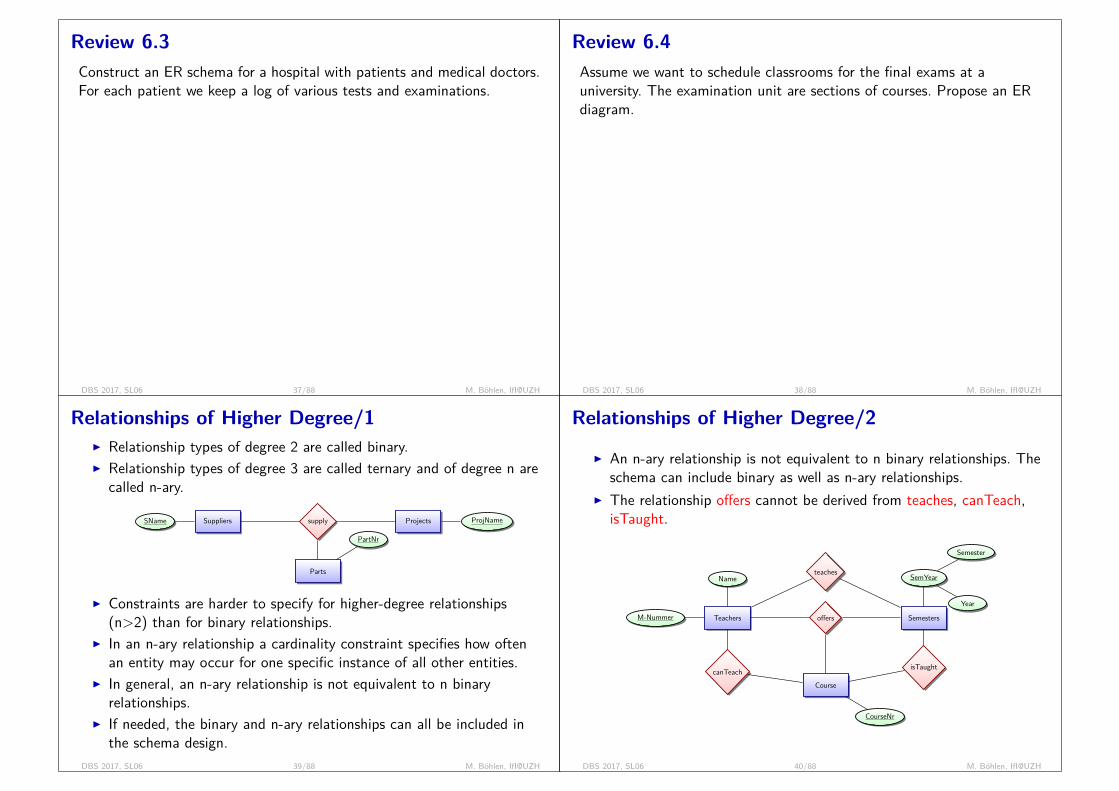
Review 6.3Construct an ER schema for a hospital with patients and medical doctors.For each patient we keep a log of various tests and examinations.
Patients
haveMedRec treatedBy
RecordsDoctors
I attrs of Patients: SSN, Name, Insurance, StartOfInsurance; key: SSNI attrs of haveMedRec: -I attrs of Records: Time, TestName, Date, Result; key: Time+TestNameI attrs of treatedBy: -I attrs of Doctors: DocSSN, Name, Adr, Specialization; key: DocSSN
DBS 2017, SL06 37/88 M. Böhlen, IfI@UZH
Review 6.4Assume we want to schedule classrooms for the final exams at auniversity. The examination unit are sections of courses. Propose an ERdiagram.
Exams
haveSyllabus takesPlace
SectionsRooms
isPartOf
Courses
I attrs of Patients: SSN, Name,Insurance, StartOfInsurance; key:SSN
I attrs of haveMedRec: -I attrs of Records: Time,
TestName, Date, Result; key:Time+TestName
I attrs of treatedBy: -I attrs of Doctors: DocSSN, Name,
Adr, Specialization; key: DocSSN
I Courses(CNr, CName, Dept)Secs(CNr, SecNr, ExId, NrEnr)Exs(ExId, Date, Time, RId)Rooms(RId, Capac, Building)
DBS 2017, SL06 38/88 M. Böhlen, IfI@UZH
Relationships of Higher Degree/1I Relationship types of degree 2 are called binary.I Relationship types of degree 3 are called ternary and of degree n are
called n-ary.
supplySuppliersSName Projects ProjName
Parts
PartNr
I Constraints are harder to specify for higher-degree relationships(n>2) than for binary relationships.
I In an n-ary relationship a cardinality constraint specifies how oftenan entity may occur for one specific instance of all other entities.
I In general, an n-ary relationship is not equivalent to n binaryrelationships.
I If needed, the binary and n-ary relationships can all be included inthe schema design.
DBS 2017, SL06 39/88 M. Böhlen, IfI@UZH
Relationships of Higher Degree/2
I An n-ary relationship is not equivalent to n binary relationships. Theschema can include binary as well as n-ary relationships.
I The relationship offers cannot be derived from teaches, canTeach,isTaught.
offersTeachers
Name
M-Nummer Semesters
SemYear
Semester
Year
Course
CourseNr
canTeach isTaught
teaches
DBS 2017, SL06 40/88 M. Böhlen, IfI@UZH
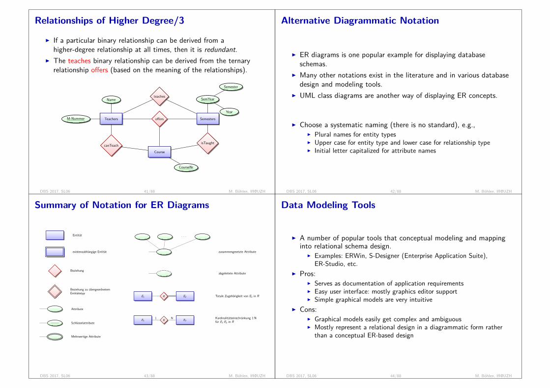
Relationships of Higher Degree/3
I If a particular binary relationship can be derived from ahigher-degree relationship at all times, then it is redundant.
I The teaches binary relationship can be derived from the ternaryrelationship offers (based on the meaning of the relationships).
offersTeachers
Name
M-Nummer Semesters
SemYear
Semester
Year
Course
CourseNr
canTeach isTaught
teaches
DBS 2017, SL06 41/88 M. Böhlen, IfI@UZH
Alternative Diagrammatic Notation
I ER diagrams is one popular example for displaying databaseschemas.
I Many other notations exist in the literature and in various databasedesign and modeling tools.
I UML class diagrams are another way of displaying ER concepts.
I Choose a systematic naming (there is no standard), e.g.,I Plural names for entity typesI Upper case for entity type and lower case for relationship typeI Initial letter capitalized for attribute names
DBS 2017, SL06 42/88 M. Böhlen, IfI@UZH
Summary of Notation for ER Diagrams
Entität
existenzabhängige Entität
Beziehung
Beziehung zu übergeordnetemEntitätstyp
Attribute
Schlüsselattribute
Mehrwertige Attribute
. . .
zusammengesetzte Attribute
abgeleitete Attribute
RE1 E2 Totale Zugehörigkeit von E2 in R
RE11 E2
N Kardinalitätseinschränkung 1:Nfür E1:E2 in R
DBS 2017, SL06 43/88 M. Böhlen, IfI@UZH
Data Modeling Tools
I A number of popular tools that conceptual modeling and mappinginto relational schema design.
I Examples: ERWin, S-Designer (Enterprise Application Suite),ER-Studio, etc.
I Pros:I Serves as documentation of application requirementsI Easy user interface: mostly graphics editor supportI Simple graphical models are very intuitive
I Cons:I Graphical models easily get complex and ambiguousI Mostly represent a relational design in a diagrammatic form rather
than a conceptual ER-based design
DBS 2017, SL06 44/88 M. Böhlen, IfI@UZH

Subclasses and Superclasses
I Sub- and SuperclassesI Disjointness Constraint (disjoint, overlapping)I Completeness Constraint (total, partial)
DBS 2017, SL06 45/88 M. Böhlen, IfI@UZH
Subclasses and Superclasses/1
I An important extension that was not present in the initial ER modelare subgroupings.
I An entity type may have additional meaningful subgroupings of itsentities
I Example: Employees may be further grouped into:I Secretaries, Engineers, Technicians, . . .
– Based on the job of an employeeI Managers
– Employees who are managersI SalariedEmps, HourlyEmps
– Based on the method of payI Extended ER diagrams represent these additional subgroupings,
called subclasses.
DBS 2017, SL06 46/88 M. Böhlen, IfI@UZH
Subclasses and Superclasses/2
I Each subgrouping is a subset of EmployeesI Each subgrouping is a subclass of EmployeesI Employees is the superclass for each of these subclassesI These are called superclass/subclass relationships:
I Employees/SecretariesI Employees/TechniciansI Employees/ManagersI . . .
I Superclass/subclass relationships are also called IS-A relationshipsI Secretaries IS-A EmployeesI Technicians IS-A EmployeesI . . .
DBS 2017, SL06 47/88 M. Böhlen, IfI@UZH
Subclasses and Superclasses/3
I An entity that is member of a subclass represents the samereal-world entity as some member of the superclass:
I The subclass member is the same entity in a distinct specific roleI An entity cannot exist in the database merely by being a member of a
subclass; it must also be a member of the superclassI A member of the superclass can be optionally included as a member
of any number of its subclassesI Examples:
I A salaried employee who is also an engineer belongs to twosubclasses:
I Engineers, andI SalariedEmps
DBS 2017, SL06 48/88 M. Böhlen, IfI@UZH

Attribute Inheritance
I An entity that is member of a subclass inheritsI All attributes of the entity as a member of the superclassI All relationships of the entity as a member of the superclass
I Example:I Secretaries (as well as Technicians and Engineers) inherit the
attributes Name, SSN, . . . , from EmployeesI Every Secretaries entity will have values for the inherited attributes
DBS 2017, SL06 49/88 M. Böhlen, IfI@UZH
Example of Subclasses and Superclasses
Secretaries Technicians Engineers Managers SalariedEmps HourlyEmps
ISA
ISAISA
Employee Name
SSNBDate
AddressFName
MInit
LName
TypingSpeed TecGrade EngType Salary
PayScale
manage
Projects
belongsTo
TradeUnion
DBS 2017, SL06 50/88 M. Böhlen, IfI@UZH
Specialization and GeneralizationI Specialization is the process of defining a set of subclasses of a
superclassI The set of subclasses is based upon some distinguishing
characteristics of the entities in the superclassI Example: SECRETARY, ENGINEER, TECHNICIAN is a
specialization of EMPLOYEE based upon job type.I We may have several specializations of the same superclassI Generalization is the reverse of the specialization processI Several classes with common features are generalized into a
superclass.I Example: CAR, TRUCK generalized into VEHICLE;
I CAR, TRUCK become subclasses of the superclass VEHICLE.I We can view {CAR, TRUCK} as a specialization of VEHICLEI Alternatively, we can view VEHICLE as a generalization of CAR and
TRUCK
DBS 2017, SL06 51/88 M. Böhlen, IfI@UZH
Constraints on Specialization/1
I Two basic constraints can apply to a specialization/generalization:I Disjointness ConstraintI Completeness Constraint
I Disjointness Constraint:I Specifies that the subclasses of the specialization must be disjoint:
I an entity can be a member of at most one of the subclasses of thespecialization
I Annotate edge in ER diagram with disjointI If not disjoint, specialization is overlapping:
I that is the same entity may be a member of more than one subclassof the specialization
I Annotate edge in ER diagram with overlapping (or no annotation)
DBS 2017, SL06 52/88 M. Böhlen, IfI@UZH
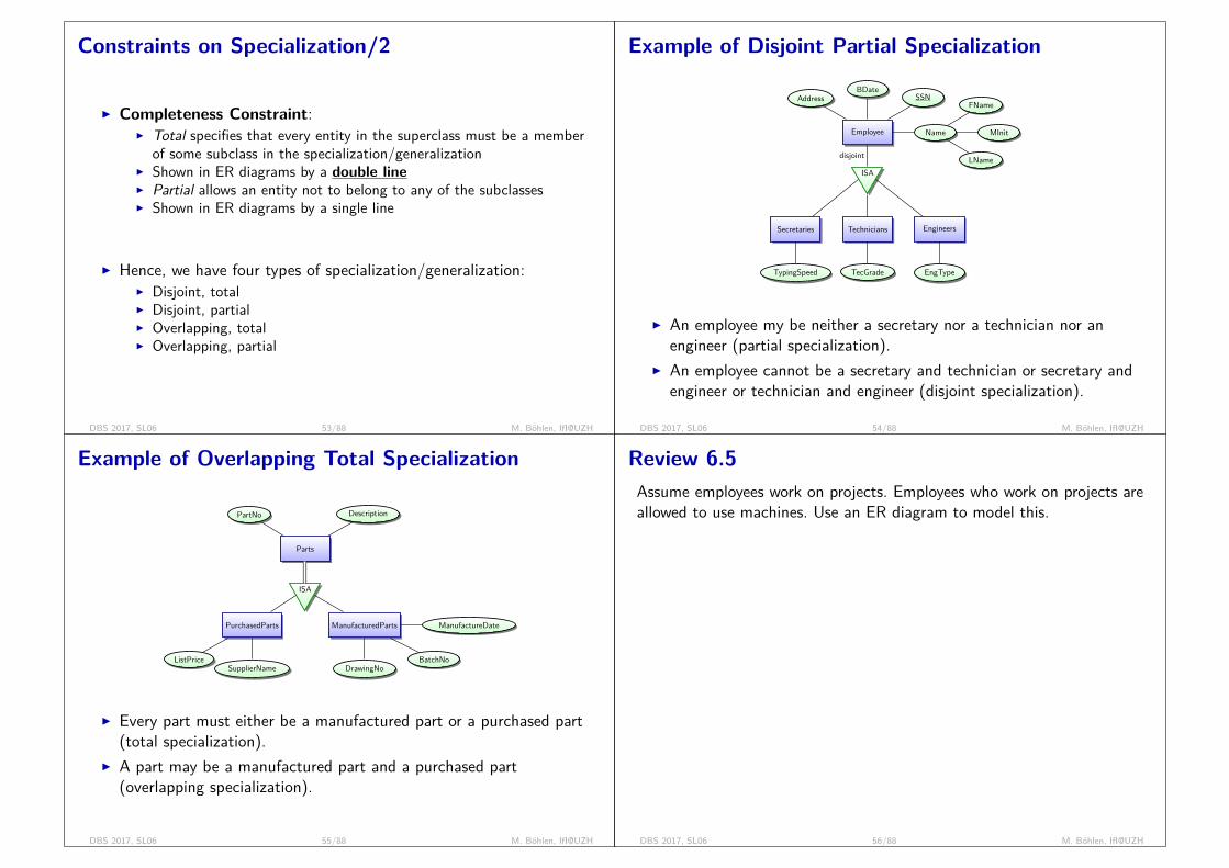
Constraints on Specialization/2
I Completeness Constraint:I Total specifies that every entity in the superclass must be a member
of some subclass in the specialization/generalizationI Shown in ER diagrams by a double lineI Partial allows an entity not to belong to any of the subclassesI Shown in ER diagrams by a single line
I Hence, we have four types of specialization/generalization:I Disjoint, totalI Disjoint, partialI Overlapping, totalI Overlapping, partial
DBS 2017, SL06 53/88 M. Böhlen, IfI@UZH
Example of Disjoint Partial Specialization
Secretaries Technicians Engineers
ISA
Employee
disjoint
Name
SSNBDate
AddressFName
MInit
LName
TypingSpeed TecGrade EngType
I An employee my be neither a secretary nor a technician nor anengineer (partial specialization).
I An employee cannot be a secretary and technician or secretary andengineer or technician and engineer (disjoint specialization).
DBS 2017, SL06 54/88 M. Böhlen, IfI@UZH
Example of Overlapping Total Specialization
Parts
PartNo Description
ISA
ManufacturedPartsPurchasedParts
DrawingNoBatchNo
ManufactureDate
SupplierNameListPrice
I Every part must either be a manufactured part or a purchased part(total specialization).
I A part may be a manufactured part and a purchased part(overlapping specialization).
DBS 2017, SL06 55/88 M. Böhlen, IfI@UZH
Review 6.5Assume employees work on projects. Employees who work on projects areallowed to use machines. Use an ER diagram to model this.
E
workOn
N
useN
P
N
N
M
N
workOnE N PN
A
1
use
1
M
1
EwP
workOn
N
useN
P
N
N
M
N
EwoP
ISA
E
disjoint
DBS 2017, SL06 56/88 M. Böhlen, IfI@UZH

ER-to-Relational MappingAlgorithm
I Mapping an ER Model to a Relational Model
DBS 2017, SL06 57/88 M. Böhlen, IfI@UZH
ER-to-Relational Mapping Algorithm/1
I Algorithm to map a conceptual database design to a relationaldatabase design.
I ER-to-Relational Mapping AlgorithmI Step 1: Mapping of Regular Entity TypesI Step 2: Mapping of Weak Entity TypesI Step 3: Mapping of Binary 1:1 Relation TypesI Step 4: Mapping of Binary 1:N Relationship TypesI Step 5: Mapping of Binary M:N Relationship TypesI Step 6: Mapping of Multivalued attributesI Step 7: Mapping of N-ary Relationship TypesI Step 8: Mapping Specialization or Generalization
DBS 2017, SL06 58/88 M. Böhlen, IfI@UZH
The ER schema for the COMPANY database
Employees
Ssn
Bdate Name
FnameMinit
Lname
Address Salary
Sex
supervise
Supervisee
N
Supervisor
1
workForN
manage1
Start_date
Departments
1
1
NameLocations
Number
NrOfEmps
control
1
workOn
M Hours
Projects
N
N
Name NumberLocation
dependentsOf
1
Dependents
N
Name Sex Birth_date Relationship
DBS 2017, SL06 59/88 M. Böhlen, IfI@UZH
ER-to-Relational Mapping Algorithm/2
I Step 1: Mapping of Regular Entity Types.I For each regular (strong) entity type E in the ER schema, create a
relation schema R that includes all the simple attributes of E.I A composite attribute is flattened into a set of simple attributes.I Choose one of the key attributes of E as the primary key for R.I If the chosen key of E is composite, the set of simple attributes that
form it will together form the primary key of R.
DBS 2017, SL06 60/88 M. Böhlen, IfI@UZH
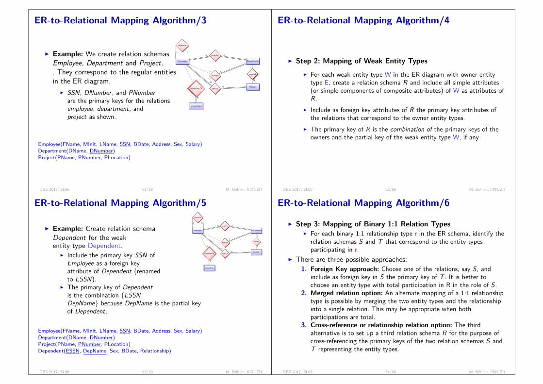
ER-to-Relational Mapping Algorithm/3
Employees
supervise
N1workForN
manage1
Departments
1
1control
1
workOn
M
Projects
N
NdependentOf
1
Dependents
N
I Example: We create relation schemasEmployee, Department and Project.. They correspond to the regular entitiesin the ER diagram.
I SSN, DNumber , and PNumberare the primary keys for the relationsemployee, department, andproject as shown.
Employee(FName, MInit, LName, SSN, BDate, Address, Sex, Salary)Department(DName, DNumber)Project(PName, PNumber, PLocation)
DBS 2017, SL06 61/88 M. Böhlen, IfI@UZH
ER-to-Relational Mapping Algorithm/4
I Step 2: Mapping of Weak Entity TypesI For each weak entity type W in the ER diagram with owner entity
type E, create a relation schema R and include all simple attributes(or simple components of composite attributes) of W as attributes ofR.
I Include as foreign key attributes of R the primary key attributes ofthe relations that correspond to the owner entity types.
I The primary key of R is the combination of the primary keys of theowners and the partial key of the weak entity type W, if any.
DBS 2017, SL06 62/88 M. Böhlen, IfI@UZH
ER-to-Relational Mapping Algorithm/5
Employees
supervise
N1workForN
manage1
Departments
1
1control
1
workOn
M
Projects
N
NdependentOf
1
Dependents
N
I Example: Create relation schemaDependent for the weakentity type Dependent.
I Include the primary key SSN ofEmployee as a foreign keyattribute of Dependent (renamedto ESSN).
I The primary key of Dependentis the combination {ESSN,DepName} because DepName is the partial keyof Dependent.
Employee(FName, MInit, LName, SSN, BDate, Address, Sex, Salary)Department(DName, DNumber)Project(PName, PNumber, PLocation)Dependent(ESSN, DepName, Sex, BDate, Relationship)
DBS 2017, SL06 63/88 M. Böhlen, IfI@UZH
ER-to-Relational Mapping Algorithm/6
I Step 3: Mapping of Binary 1:1 Relation TypesI For each binary 1:1 relationship type r in the ER schema, identify the
relation schemas S and T that correspond to the entity typesparticipating in r.
I There are three possible approaches:1. Foreign Key approach: Choose one of the relations, say S, and
include as foreign key in S the primary key of T . It is better tochoose an entity type with total participation in R in the role of S.
2. Merged relation option: An alternate mapping of a 1:1 relationshiptype is possible by merging the two entity types and the relationshipinto a single relation. This may be appropriate when bothparticipations are total.
3. Cross-reference or relationship relation option: The thirdalternative is to set up a third relation schema R for the purpose ofcross-referencing the primary keys of the two relation schemas S andT representing the entity types.
DBS 2017, SL06 64/88 M. Böhlen, IfI@UZH

ER-to-Relational Mapping Algorithm/7
Employees
supervise
N1workForN
manage1
Departments
1
1control
1
workOn
M
Projects
N
NdependentOf
1
Dependents
N
I Example: The 1:1 relation manageis mapped by choosing the participatingentity type Department to serve in therole of S, because its participation in themanage relationship type is total.
Employee(FName, MInit, LName, SSN, BDate, Address, Sex, Salary)Department(DName, DNumber, MgrSSN, MgrStartDate)Project(PName, PNumber, PLocation)Dependent(ESSN, DepName, Sex, BDate, Relationship)
DBS 2017, SL06 65/88 M. Böhlen, IfI@UZH
Review 6.6Illustrate the problems that occur if the 1:1 relationship manage ismapped through a foreign key in relation schema Employee.
good solution (no NULL values):department = { (’ifi’, 4, GlinzAHV, 2009), (’ibw’, 2, PfaffAHV, 2011) }employee = { (’Glinz’, ...), (’Stiller’, ...), (’Pfaff’, ...) }
bad solution (many NULL values):department = { (’ifi’,4), (’ibw’,2) }employee = { (’Glinz’, ..., GlinzAHV, 2009), (’Stiller’, ..., NULL, NULL), (’Pfaff’, ...,PfaffAHV, 2011) }
DBS 2017, SL06 66/88 M. Böhlen, IfI@UZH
ER-to-Relational Mapping Algorithm/8
I Step 4: Mapping of Binary 1:N Relationship TypesI For each binary 1:N relationship type r, identify the relation schemas
S and T that correspond to the entity types participating in r. S isthe N-side.
I Include as foreign key in S the primary key of T that represents theother entity type participating in r.
I Include simple attributes of the 1:N relation type as attributes of S.
DBS 2017, SL06 67/88 M. Böhlen, IfI@UZH
ER-to-Relational Mapping Algorithm/9
Employees
supervise
N1workForN
manage1
Departments
1
1control
1
workOn
M
Projects
N
NdependentOf
1
Dependents
N
I Example: 1:N relationship typesworkFor, control and supervise.
I For example for workFor weinclude the primary key DNumberof the Department relation schemaas foreign key in the Employeerelation schema and call it DNo.
Employee(FName, MInit, LName, SSN, BDate, Address, Sex, Salary, SuperSSN, DNo)Department(DName, DNumber, MgrSSN, MgrStartDate)Project(PName, PNumber, PLocation, DNum)Dependent(ESSN, DepName, Sex, BDate, Relationship)
DBS 2017, SL06 68/88 M. Böhlen, IfI@UZH
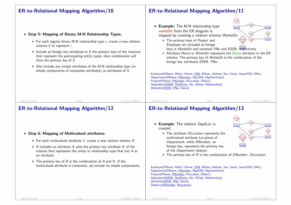
ER-to-Relational Mapping Algorithm/10
I Step 5: Mapping of Binary M:N Relationship Types.I For each regular binary M:N relationship type r, create a new relation
schema S to represent r.I Include as foreign key attributes in S the primary keys of the relations
that represent the participating entity types; their combination willform the primary key of S.
I Also include any simple attributes of the M:N relationship type (orsimple components of composite attributes) as attributes of S.
DBS 2017, SL06 69/88 M. Böhlen, IfI@UZH
ER-to-Relational Mapping Algorithm/11
Employees
supervise
N1workForN
manage1
Departments
1
1control
1
workOn
M
Projects
N
NdependentOf
1
Dependents
N
I Example: The M:N relationship typeworksOn from the ER diagram ismapped by creating a relation schema WorksOn.
I The primary keys of Project andEmployee are included as foreignkeys in WorksOn and renamed PNo and ESSN, respectively.
I Attribute Hours in WorksOn represents the Hours attribute in the ERschema. The primary key of WorksOn is the combination of theforeign key attributes ESSN, PNo.
Employee(FName, MInit, LName, SSN, BDate, Address, Sex, Salary, SuperSSN, DNo)Department(DName, DNumber, MgrSSN, MgrStartDate)Project(PName, PNumber, PLocation, DNum)Dependent(ESSN, DepName, Sex, BDate, Relationship)WorksOn(ESSN, PNo, Hours)
DBS 2017, SL06 70/88 M. Böhlen, IfI@UZH
ER-to-Relational Mapping Algorithm/12
I Step 6: Mapping of Multivalued attributes.I For each multivalued attribute A, create a new relation schema R.I R includes an attribute A, plus the primary key attribute K of the
relation that represents the entity or relationship type that has A asan attribute.
I The primary key of R is the combination of A and K . If themultivalued attribute is composite, we include its simple components.
DBS 2017, SL06 71/88 M. Böhlen, IfI@UZH
ER-to-Relational Mapping Algorithm/13
Employees
supervise
N1workForN
manage1
Departments
1
1control
1
workOn
M
Projects
N
NdependentOf
1
Dependents
N
I Example: The relation DeptLoc iscreated.
I The attribute DLocation represents themultivalued attribute Locations ofDepartment, while DNumber , asforeign key, represents the primary keyof the Department relation.
I The primary key of R is the combination of DNumber , DLocation.
Employee(FName, MInit, LName, SSN, BDate, Address, Sex, Salary, SuperSSN, DNo)Department(DName, DNumber, MgrSSN, MgrStartDate)Project(PName, PNumber, PLocation, DNum)Dependent(ESSN, DepName, Sex, BDate, Relationship)WorksOn(ESSN, PNo, Hours)DeptLoc(DNumber, DLocation)
DBS 2017, SL06 72/88 M. Böhlen, IfI@UZH
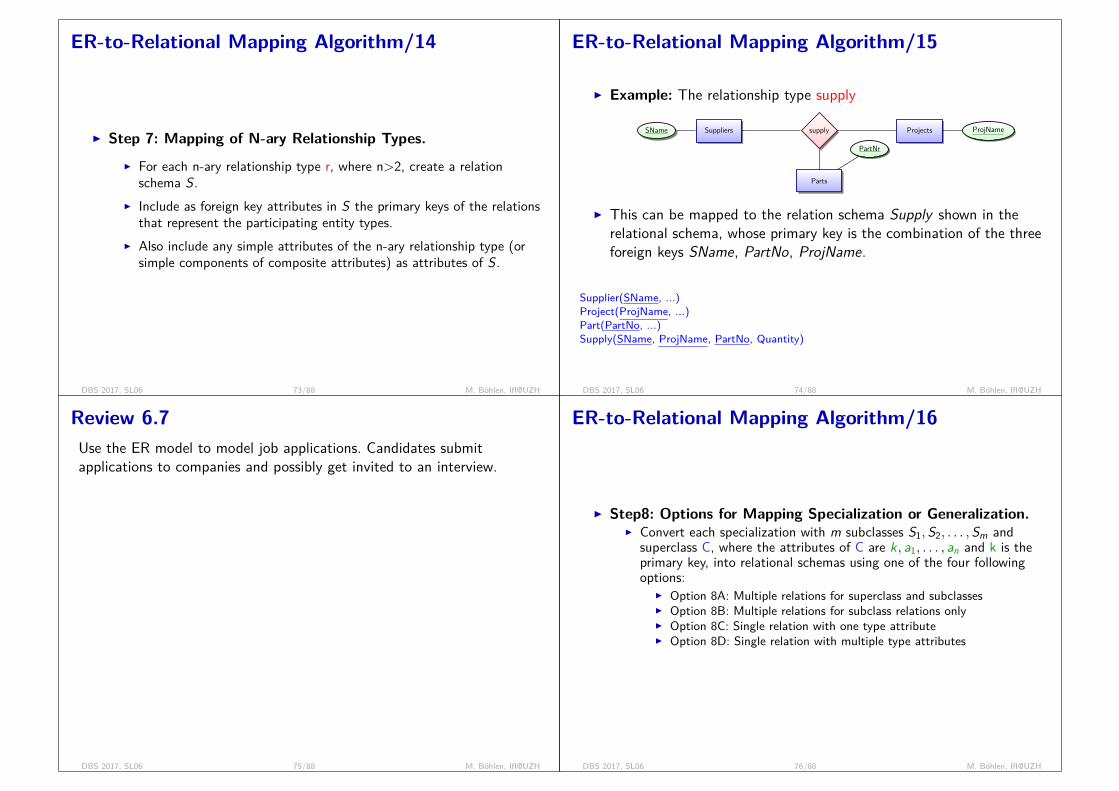
ER-to-Relational Mapping Algorithm/14
I Step 7: Mapping of N-ary Relationship Types.I For each n-ary relationship type r, where n>2, create a relation
schema S.I Include as foreign key attributes in S the primary keys of the relations
that represent the participating entity types.I Also include any simple attributes of the n-ary relationship type (or
simple components of composite attributes) as attributes of S.
DBS 2017, SL06 73/88 M. Böhlen, IfI@UZH
ER-to-Relational Mapping Algorithm/15
I Example: The relationship type supply
supplySuppliersSName Projects ProjName
Parts
PartNr
I This can be mapped to the relation schema Supply shown in therelational schema, whose primary key is the combination of the threeforeign keys SName, PartNo, ProjName.
Supplier(SName, ...)Project(ProjName, ...)Part(PartNo, ...)Supply(SName, ProjName, PartNo, Quantity)
DBS 2017, SL06 74/88 M. Böhlen, IfI@UZH
Review 6.7Use the ER model to model job applications. Candidates submitapplications to companies and possibly get invited to an interview.
appliesCands N CompsN
Interviews
1
appliesCands N CompsN
invited
1
Interviews
1
Applications
invited
1
Interviews
1
appliesCands N CompsN
Interviews
1
DBS 2017, SL06 75/88 M. Böhlen, IfI@UZH
ER-to-Relational Mapping Algorithm/16
I Step8: Options for Mapping Specialization or Generalization.I Convert each specialization with m subclasses S1, S2, . . . ,Sm and
superclass C, where the attributes of C are k, a1, . . . , an and k is theprimary key, into relational schemas using one of the four followingoptions:
I Option 8A: Multiple relations for superclass and subclassesI Option 8B: Multiple relations for subclass relations onlyI Option 8C: Single relation with one type attributeI Option 8D: Single relation with multiple type attributes
DBS 2017, SL06 76/88 M. Böhlen, IfI@UZH
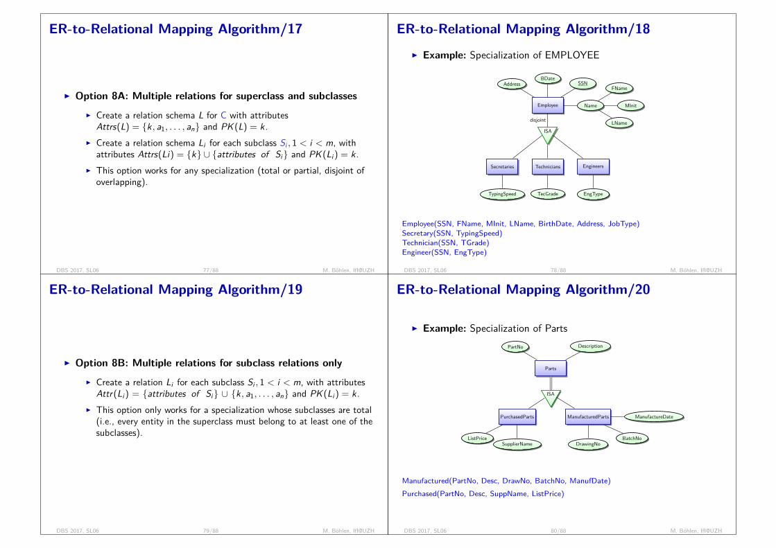
ER-to-Relational Mapping Algorithm/17
I Option 8A: Multiple relations for superclass and subclassesI Create a relation schema L for C with attributes
Attrs(L) = {k, a1, . . . , an} and PK (L) = k.I Create a relation schema Li for each subclass Si , 1 < i < m, with
attributes Attrs(Li) = {k} ∪ {attributes of Si} and PK (Li) = k.I This option works for any specialization (total or partial, disjoint of
overlapping).
DBS 2017, SL06 77/88 M. Böhlen, IfI@UZH
ER-to-Relational Mapping Algorithm/18I Example: Specialization of EMPLOYEE
Secretaries Technicians Engineers
ISA
Employee
disjoint
Name
SSNBDate
AddressFName
MInit
LName
TypingSpeed TecGrade EngType
Employee(SSN, FName, MInit, LName, BirthDate, Address, JobType)Secretary(SSN, TypingSpeed)Technician(SSN, TGrade)Engineer(SSN, EngType)
DBS 2017, SL06 78/88 M. Böhlen, IfI@UZH
ER-to-Relational Mapping Algorithm/19
I Option 8B: Multiple relations for subclass relations onlyI Create a relation Li for each subclass Si , 1 < i < m, with attributes
Attr(Li) = {attributes of Si} ∪ {k, a1, . . . , an} and PK (Li) = k.I This option only works for a specialization whose subclasses are total
(i.e., every entity in the superclass must belong to at least one of thesubclasses).
DBS 2017, SL06 79/88 M. Böhlen, IfI@UZH
ER-to-Relational Mapping Algorithm/20
I Example: Specialization of Parts
Parts
PartNo Description
ISA
ManufacturedPartsPurchasedParts
DrawingNoBatchNo
ManufactureDate
SupplierNameListPrice
Manufactured(PartNo, Desc, DrawNo, BatchNo, ManufDate)Purchased(PartNo, Desc, SuppName, ListPrice)
DBS 2017, SL06 80/88 M. Böhlen, IfI@UZH
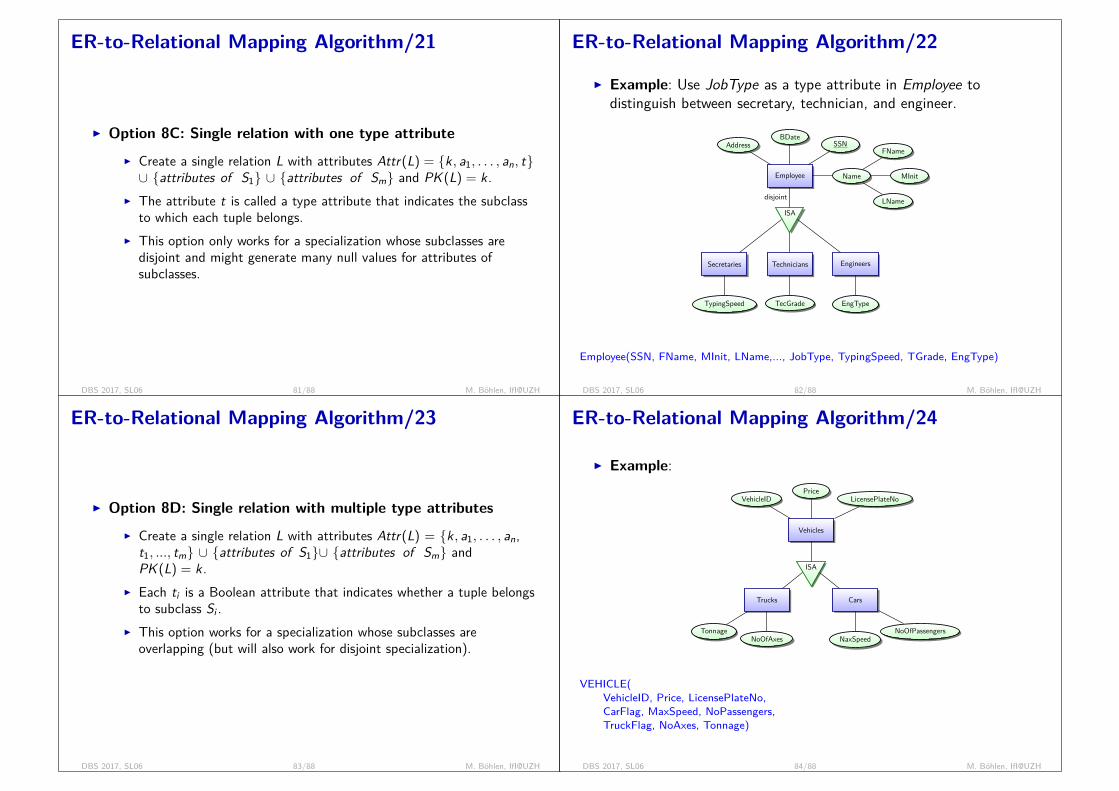
ER-to-Relational Mapping Algorithm/21
I Option 8C: Single relation with one type attributeI Create a single relation L with attributes Attr(L) = {k, a1, . . . , an, t}
∪ {attributes of S1} ∪ {attributes of Sm} and PK (L) = k.I The attribute t is called a type attribute that indicates the subclass
to which each tuple belongs.I This option only works for a specialization whose subclasses are
disjoint and might generate many null values for attributes ofsubclasses.
DBS 2017, SL06 81/88 M. Böhlen, IfI@UZH
ER-to-Relational Mapping Algorithm/22
I Example: Use JobType as a type attribute in Employee todistinguish between secretary, technician, and engineer.
Secretaries Technicians Engineers
ISA
Employee
disjoint
Name
SSNBDate
AddressFName
MInit
LName
TypingSpeed TecGrade EngType
Employee(SSN, FName, MInit, LName,..., JobType, TypingSpeed, TGrade, EngType)
DBS 2017, SL06 82/88 M. Böhlen, IfI@UZH
ER-to-Relational Mapping Algorithm/23
I Option 8D: Single relation with multiple type attributesI Create a single relation L with attributes Attr(L) = {k, a1, . . . , an,
t1, ..., tm} ∪ {attributes of S1}∪ {attributes of Sm} andPK (L) = k.
I Each ti is a Boolean attribute that indicates whether a tuple belongsto subclass Si .
I This option works for a specialization whose subclasses areoverlapping (but will also work for disjoint specialization).
DBS 2017, SL06 83/88 M. Böhlen, IfI@UZH
ER-to-Relational Mapping Algorithm/24
I Example:
Vehicles
VehicleIDPrice
LicensePlateNo
ISA
CarsTrucks
NaxSpeedNoOfPassengers
NoOfAxesTonnage
VEHICLE(VehicleID, Price, LicensePlateNo,CarFlag, MaxSpeed, NoPassengers,TruckFlag, NoAxes, Tonnage)
DBS 2017, SL06 84/88 M. Böhlen, IfI@UZH

ER-to-Relational Mapping Algorithm/27
DBS 2017, SL06 85/88 M. Böhlen, IfI@UZH
Summary of Mapping Constructs and Constraints
Correspondence between ER and Relational Models
ER Model Relational ModelEntity type Entity relation1:1 or 1:N relationship type Foreign key (or relationship relation)M:N relationship type Relationship relation and two foreign keysn-ary relationship type Relationship relation and n foreign keysSimple attribute AttributeComposite attribute Set of simple component attributesMultivalued attribute Relation and foreign keyKey attribute Primary (or secondary) key
DBS 2017, SL06 86/88 M. Böhlen, IfI@UZH
Summary/1
I ER model concepts:I entity type, entity set, entityI attribute, attribute valueI relationship type, relationship set, relationshipI structural constraints: cardinality, participationI subclasses and superclasses
I During the conceptual modeling process a number of clarifyingdecisions/assumptions must be made
I It is important to make all necessary decisions (even if alternativesexist) and go on. Make decisions explicit (i.e., write them down).
I There is not a unique ER model.I In order to clarify the semantics it can hep to consider relation
instances
DBS 2017, SL06 87/88 M. Böhlen, IfI@UZH
Summary/2
I ER-to-Relational Mapping AlgorithmI Step 1: Mapping of Regular Entity TypesI Step 2: Mapping of Weak Entity TypesI Step 3: Mapping of Binary 1:1 Relation TypesI Step 4: Mapping of Binary 1:N Relationship Types.I Step 5: Mapping of Binary M:N Relationship Types.I Step 6: Mapping of Multivalued attributes.I Step 7: Mapping of N-ary Relationship Types.I Step 8: Mapping Specialization or Generalization.
I The mapping algorithm is mechanical and without conceptualdifficulty. Make sure you know how to apply it.
DBS 2017, SL06 88/88 M. Böhlen, IfI@UZH
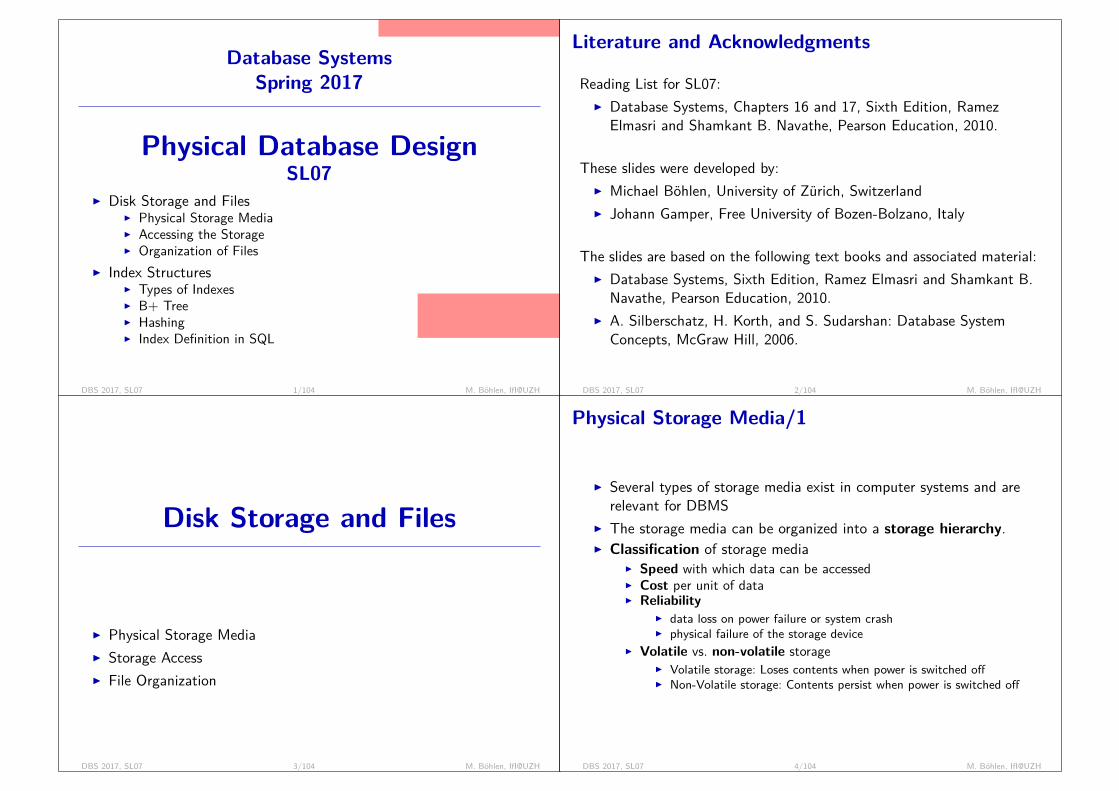
Database SystemsSpring 2017
Physical Database DesignSL07
I Disk Storage and FilesI Physical Storage MediaI Accessing the StorageI Organization of Files
I Index StructuresI Types of IndexesI B+ TreeI HashingI Index Definition in SQL
Reviews: 15 20 26 37 48 71 78 95
Verwaltung des Speichers:- OS files (PostgreSQL)- raw disk (Oracle)
DBS 2017, SL07 1/104 M. Böhlen, IfI@UZH
Literature and Acknowledgments
Reading List for SL07:I Database Systems, Chapters 16 and 17, Sixth Edition, Ramez
Elmasri and Shamkant B. Navathe, Pearson Education, 2010.
These slides were developed by:I Michael Böhlen, University of Zürich, SwitzerlandI Johann Gamper, Free University of Bozen-Bolzano, Italy
The slides are based on the following text books and associated material:I Database Systems, Sixth Edition, Ramez Elmasri and Shamkant B.
Navathe, Pearson Education, 2010.I A. Silberschatz, H. Korth, and S. Sudarshan: Database System
Concepts, McGraw Hill, 2006.
DBS 2017, SL07 2/104 M. Böhlen, IfI@UZH
Disk Storage and Files
I Physical Storage MediaI Storage AccessI File Organization
DBS 2017, SL07 3/104 M. Böhlen, IfI@UZH
Physical Storage Media/1
I Several types of storage media exist in computer systems and arerelevant for DBMS
I The storage media can be organized into a storage hierarchy.I Classification of storage media
I Speed with which data can be accessedI Cost per unit of dataI Reliability
I data loss on power failure or system crashI physical failure of the storage device
I Volatile vs. non-volatile storageI Volatile storage: Loses contents when power is switched offI Non-Volatile storage: Contents persist when power is switched off
DBS 2017, SL07 4/104 M. Böhlen, IfI@UZH
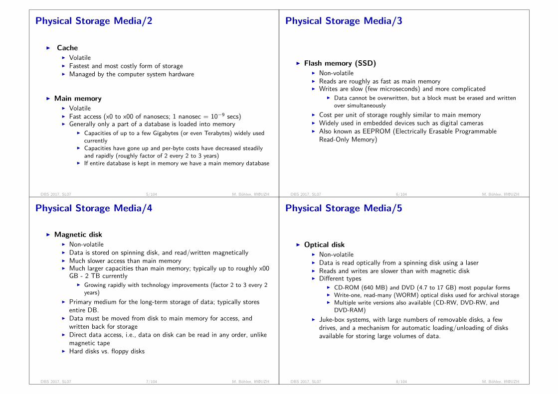
Physical Storage Media/2
I CacheI VolatileI Fastest and most costly form of storageI Managed by the computer system hardware
I Main memoryI VolatileI Fast access (x0 to x00 of nanosecs; 1 nanosec = 10−9 secs)I Generally only a part of a database is loaded into memory
I Capacities of up to a few Gigabytes (or even Terabytes) widely usedcurrently
I Capacities have gone up and per-byte costs have decreased steadilyand rapidly (roughly factor of 2 every 2 to 3 years)
I If entire database is kept in memory we have a main memory database
DBS 2017, SL07 5/104 M. Böhlen, IfI@UZH
Physical Storage Media/3
I Flash memory (SSD)I Non-volatileI Reads are roughly as fast as main memoryI Writes are slow (few microseconds) and more complicated
I Data cannot be overwritten, but a block must be erased and writtenover simultaneously
I Cost per unit of storage roughly similar to main memoryI Widely used in embedded devices such as digital camerasI Also known as EEPROM (Electrically Erasable Programmable
Read-Only Memory)
DBS 2017, SL07 6/104 M. Böhlen, IfI@UZH
Physical Storage Media/4
I Magnetic diskI Non-volatileI Data is stored on spinning disk, and read/written magneticallyI Much slower access than main memoryI Much larger capacities than main memory; typically up to roughly x00
GB - 2 TB currentlyI Growing rapidly with technology improvements (factor 2 to 3 every 2
years)I Primary medium for the long-term storage of data; typically stores
entire DB.I Data must be moved from disk to main memory for access, and
written back for storageI Direct data access, i.e., data on disk can be read in any order, unlike
magnetic tapeI Hard disks vs. floppy disks
DBS 2017, SL07 7/104 M. Böhlen, IfI@UZH
Physical Storage Media/5
I Optical diskI Non-volatileI Data is read optically from a spinning disk using a laserI Reads and writes are slower than with magnetic diskI Different types
I CD-ROM (640 MB) and DVD (4.7 to 17 GB) most popular formsI Write-one, read-many (WORM) optical disks used for archival storageI Multiple write versions also available (CD-RW, DVD-RW, and
DVD-RAM)I Juke-box systems, with large numbers of removable disks, a few
drives, and a mechanism for automatic loading/unloading of disksavailable for storing large volumes of data.
DBS 2017, SL07 8/104 M. Böhlen, IfI@UZH
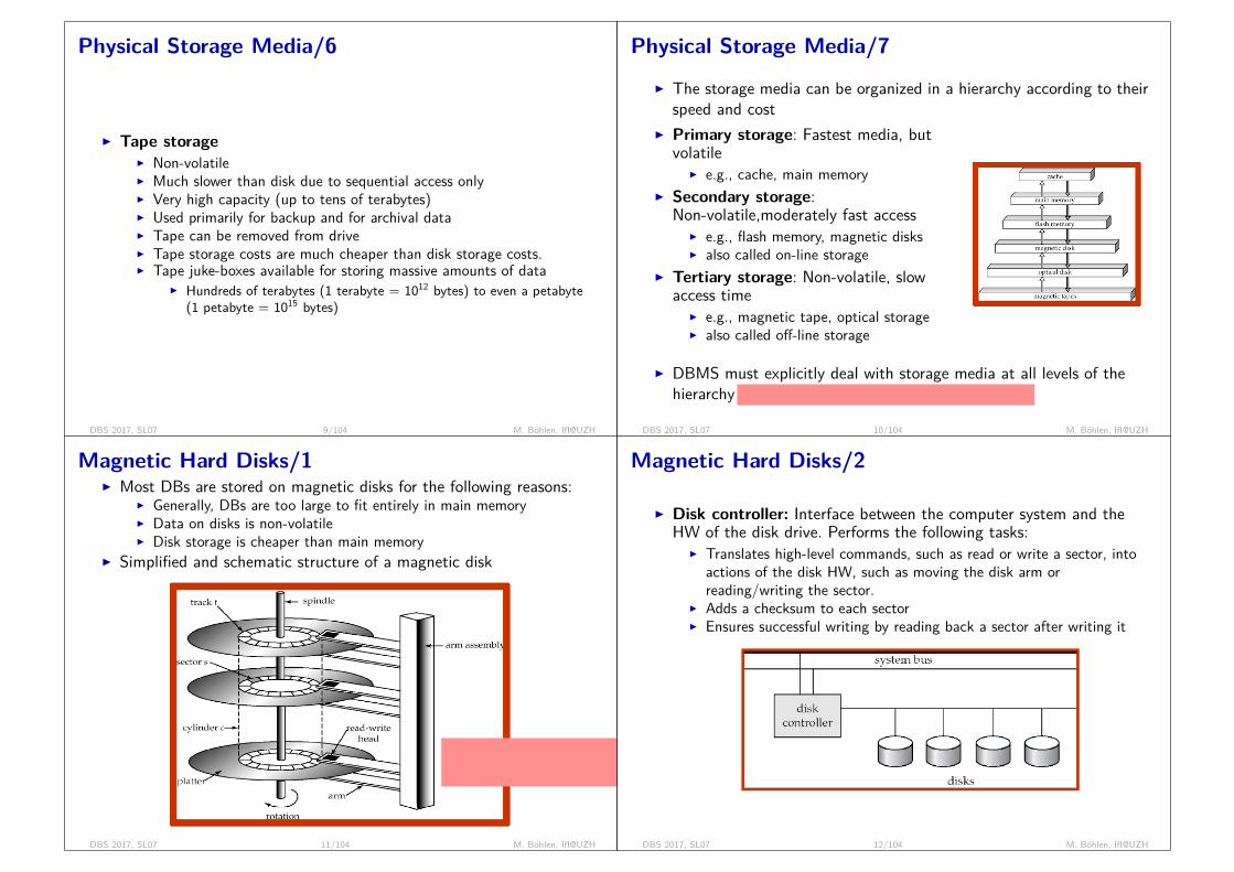
Physical Storage Media/6
I Tape storageI Non-volatileI Much slower than disk due to sequential access onlyI Very high capacity (up to tens of terabytes)I Used primarily for backup and for archival dataI Tape can be removed from driveI Tape storage costs are much cheaper than disk storage costs.I Tape juke-boxes available for storing massive amounts of data
I Hundreds of terabytes (1 terabyte = 1012 bytes) to even a petabyte(1 petabyte = 1015 bytes)
DBS 2017, SL07 9/104 M. Böhlen, IfI@UZH
Physical Storage Media/7I The storage media can be organized in a hierarchy according to their
speed and costI Primary storage: Fastest media, but
volatileI e.g., cache, main memory
I Secondary storage:Non-volatile,moderately fast access
I e.g., flash memory, magnetic disksI also called on-line storage
I Tertiary storage: Non-volatile, slowaccess time
I e.g., magnetic tape, optical storageI also called off-line storage
I DBMS must explicitly deal with storage media at all levels of thehierarchy
phone book, library, encycopedia, Google, Wikipedia
DBS 2017, SL07 10/104 M. Böhlen, IfI@UZH
Magnetic Hard Disks/1I Most DBs are stored on magnetic disks for the following reasons:
I Generally, DBs are too large to fit entirely in main memoryI Data on disks is non-volatileI Disk storage is cheaper than main memory
I Simplified and schematic structure of a magnetic disk
choosing a different disk ischeap (electronic switch); mo-ving disk head is expensive
DBS 2017, SL07 11/104 M. Böhlen, IfI@UZH
Magnetic Hard Disks/2
I Disk controller: Interface between the computer system and theHW of the disk drive. Performs the following tasks:
I Translates high-level commands, such as read or write a sector, intoactions of the disk HW, such as moving the disk arm orreading/writing the sector.
I Adds a checksum to each sectorI Ensures successful writing by reading back a sector after writing it
DBS 2017, SL07 12/104 M. Böhlen, IfI@UZH
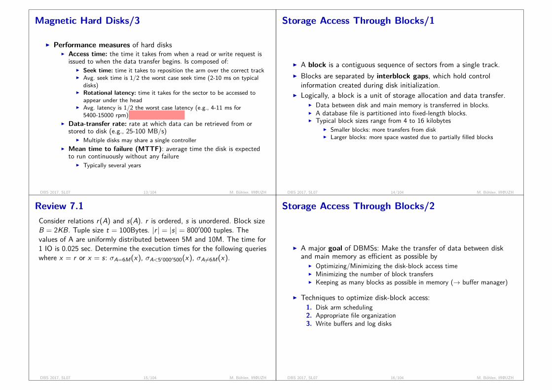
Magnetic Hard Disks/3
I Performance measures of hard disksI Access time: the time it takes from when a read or write request is
issued to when the data transfer begins. Is composed of:I Seek time: time it takes to reposition the arm over the correct trackI Avg. seek time is 1/2 the worst case seek time (2-10 ms on typical
disks)I Rotational latency: time it takes for the sector to be accessed to
appear under the headI Avg. latency is 1/2 the worst case latency (e.g., 4-11 ms for
5400-15000 rpm)
rotations per minute
I Data-transfer rate: rate at which data can be retrieved from orstored to disk (e.g., 25-100 MB/s)
I Multiple disks may share a single controllerI Mean time to failure (MTTF): average time the disk is expected
to run continuously without any failureI Typically several years
DBS 2017, SL07 13/104 M. Böhlen, IfI@UZH
Storage Access Through Blocks/1
I A block is a contiguous sequence of sectors from a single track.I Blocks are separated by interblock gaps, which hold control
information created during disk initialization.I Logically, a block is a unit of storage allocation and data transfer.
I Data between disk and main memory is transferred in blocks.I A database file is partitioned into fixed-length blocks.I Typical block sizes range from 4 to 16 kilobytes
I Smaller blocks: more transfers from diskI Larger blocks: more space wasted due to partially filled blocks
DBS 2017, SL07 14/104 M. Böhlen, IfI@UZH
Review 7.1Consider relations r(A) and s(A). r is ordered, s is unordered. Block sizeB = 2KB. Tuple size t = 100Bytes. |r | = |s| = 800′000 tuples. Thevalues of A are uniformly distributed between 5M and 10M. The time for1 IO is 0.025 sec. Determine the execution times for the following querieswhere x = r or x = s: σA=6M(x), σA<5′000′500(x), σA6=6M(x).
I 2K/100 = 20 tuples/blockI 800’000/20 = 40’000 blocksI σA=6M(r): binary search on contiguous blocks 0.025 ∗ lg 40′000secI σA=6M(s): scan half of s on avg if A is unique 0.025 ∗ 20′000 = 500secI σA<5′000′500(r):
I avg distance between values = 5M/800′000 = 6.25I nr of qualifying tuples = 500/6.25 = 80I nr of qualifying blocks = d80/20e = 4I 0.025 ∗ 4 = 0.1sec
I σA<5′000′500(s): 0.025 ∗ 40′000 = 1000secI σA6=6M(.): scan relation 0.025 ∗ 40′000 = 1000sec
DBS 2017, SL07 15/104 M. Böhlen, IfI@UZH
Storage Access Through Blocks/2
I A major goal of DBMSs: Make the transfer of data between diskand main memory as efficient as possible by
I Optimizing/Minimizing the disk-block access timeI Minimizing the number of block transfersI Keeping as many blocks as possible in memory (→ buffer manager)
I Techniques to optimize disk-block access:1. Disk arm scheduling2. Appropriate file organization3. Write buffers and log disks
DBS 2017, SL07 16/104 M. Böhlen, IfI@UZH
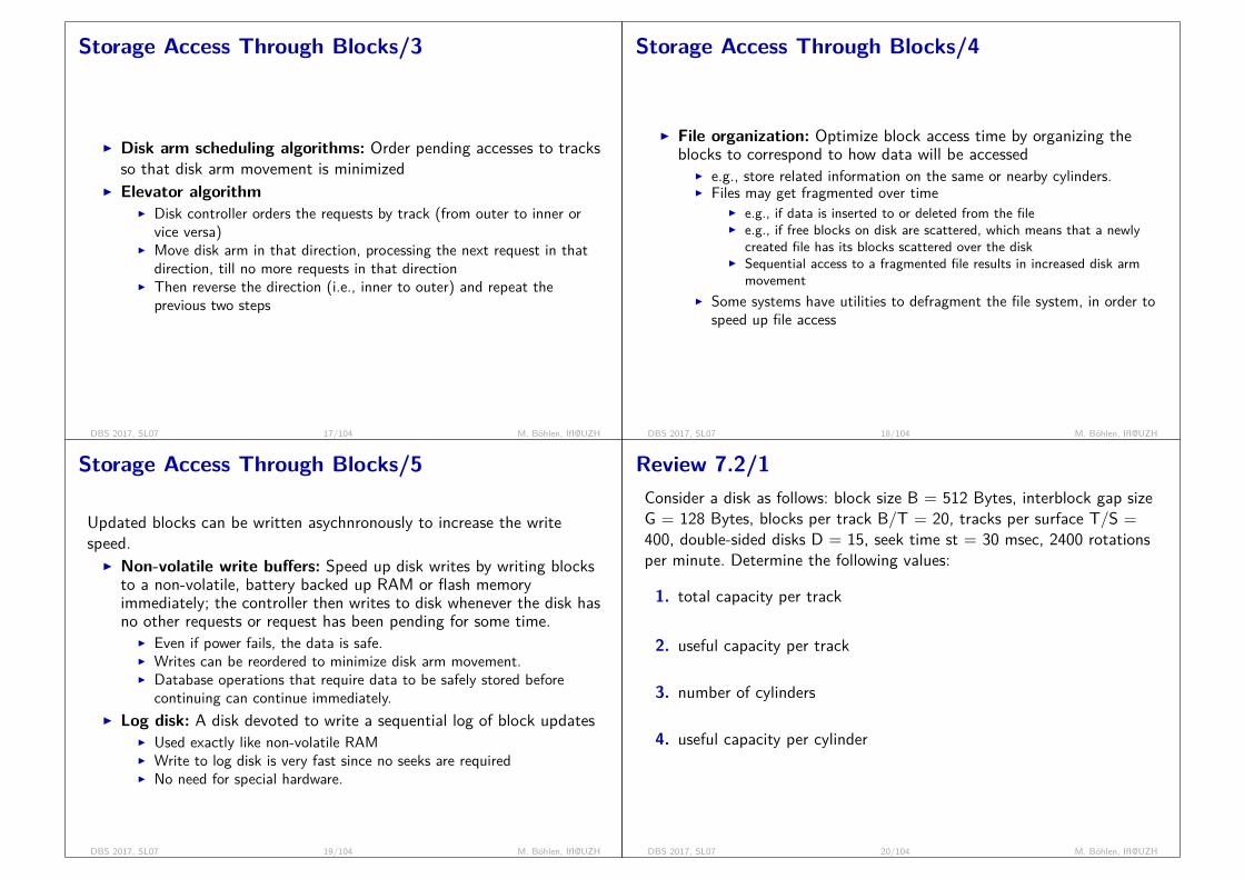
Storage Access Through Blocks/3
I Disk arm scheduling algorithms: Order pending accesses to tracksso that disk arm movement is minimized
I Elevator algorithmI Disk controller orders the requests by track (from outer to inner or
vice versa)I Move disk arm in that direction, processing the next request in that
direction, till no more requests in that directionI Then reverse the direction (i.e., inner to outer) and repeat the
previous two steps
DBS 2017, SL07 17/104 M. Böhlen, IfI@UZH
Storage Access Through Blocks/4
I File organization: Optimize block access time by organizing theblocks to correspond to how data will be accessed
I e.g., store related information on the same or nearby cylinders.I Files may get fragmented over time
I e.g., if data is inserted to or deleted from the fileI e.g., if free blocks on disk are scattered, which means that a newly
created file has its blocks scattered over the diskI Sequential access to a fragmented file results in increased disk arm
movementI Some systems have utilities to defragment the file system, in order to
speed up file access
DBS 2017, SL07 18/104 M. Böhlen, IfI@UZH
Storage Access Through Blocks/5
Updated blocks can be written asychnronously to increase the writespeed.
I Non-volatile write buffers: Speed up disk writes by writing blocksto a non-volatile, battery backed up RAM or flash memoryimmediately; the controller then writes to disk whenever the disk hasno other requests or request has been pending for some time.
I Even if power fails, the data is safe.I Writes can be reordered to minimize disk arm movement.I Database operations that require data to be safely stored before
continuing can continue immediately.I Log disk: A disk devoted to write a sequential log of block updates
I Used exactly like non-volatile RAMI Write to log disk is very fast since no seeks are requiredI No need for special hardware.
DBS 2017, SL07 19/104 M. Böhlen, IfI@UZH
Review 7.2/1Consider a disk as follows: block size B = 512 Bytes, interblock gap sizeG = 128 Bytes, blocks per track B/T = 20, tracks per surface T/S =400, double-sided disks D = 15, seek time st = 30 msec, 2400 rotationsper minute. Determine the following values:
1. total capacity per track
20 *(512 + 128) = 12.8 KB
2. useful capacity per track
20 * 512 = 10.24 KB
3. number of cylinders
= number of tracks = 400
4. useful capacity per cylinder
2 * 15 * 10.24 = 307KB
DBS 2017, SL07 20/104 M. Böhlen, IfI@UZH
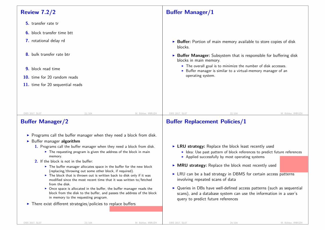
Review 7.2/2
5. transfer rate tr
tr = 12’000 * 2400/(60*1000) = 512 Bytes/msec
6. block transfer time btt
btt = B/tr = 512/512 = 1msec
7. rotational delay rd
rd = 0.5 * (60 * 1000 / 2400) = 12.5msec (time for half a rotation)
8. bulk transfer rate btr
btr = tr *(B/B+G) = 512 * 0.8 = 409.6 Bytes/msec
9. block read time
st + rd + btt = 30 + 12.5 + 1 = 43.5msec
10. time for 20 random reads
20 * 43.5 = 870msec
11. time for 20 sequential reads
20 * btt + st + rd = 62.5msec [or 20 * B/btr + st + rd = 67.5]
DBS 2017, SL07 21/104 M. Böhlen, IfI@UZH
Buffer Manager/1
I Buffer: Portion of main memory available to store copies of diskblocks.
I Buffer Manager: Subsystem that is responsible for buffering diskblocks in main memory.
I The overall goal is to minimize the number of disk accesses.I Buffer manager is similar to a virtual-memory manager of an
operating system.
DBS 2017, SL07 22/104 M. Böhlen, IfI@UZH
Buffer Manager/2
I Programs call the buffer manager when they need a block from disk.I Buffer manager algorithm
1. Programs call the buffer manager when they need a block from disk.I The requesting program is given the address of the block in main
memory.2. If the block is not in the buffer:
I The buffer manager allocates space in the buffer for the new block(replacing/throwing out some other block, if required).
I The block that is thrown out is written back to disk only if it wasmodified since the most recent time that it was written to/fetchedfrom the disk.
I Once space is allocated in the buffer, the buffer manager reads theblock from the disk to the buffer, and passes the address of the blockin memory to the requesting program.
I There exist different strategies/policies to replace buffers
swapping is not an efficient option
DBS 2017, SL07 23/104 M. Böhlen, IfI@UZH
Buffer Replacement Policies/1
we know that wedo not need theblock again for along time
I LRU strategy: Replace the block least recently usedI Idea: Use past pattern of block references to predict future referencesI Applied successfully by most operating systems
I MRU strategy: Replace the block most recently used
I LRU can be a bad strategy in DBMS for certain access patternsinvolving repeated scans of data
I Queries in DBs have well-defined access patterns (such as sequentialscans), and a database system can use the information in a user’squery to predict future references
DBS 2017, SL07 24/104 M. Böhlen, IfI@UZH

Buffer Replacement Policies/2
I Example: compute a join with nested loopsfor each tuple tr of r do
for each tuple ts of s doif the tuples tr and ts match then ...;
I Different access pattern for r and sI An r-block is no longer needed, after the last tuple is processed (even
if it has been used recently), thus should be removed immediatelyI An s-block is needed again after all other s-blocks are processed, thus
MRU is the best strategyI A mixed strategy with hints on replacement strategy provided by the
query optimizer is preferable
DBS 2017, SL07 25/104 M. Böhlen, IfI@UZH
Review 7.3Assume a relation r with 3 tuples and a relation s with 3 tuples. Assumea block can fit 2 tuples. Illustrate how a nested loop join processes tuplesand how to use blocks if 2 blocks are available for the join.
r = {r1, r2, r3}, s = {s1, s2, s3}B1 B2
r1 s1 Br1 Bs1r1 s2r1 s3 Bs2r2 s1 Bs1r2 s2r2 s3 Bs2r3 s1 Br2 Bs1r3 s2r3 s3 Bs2
B1 B2r1 s1 Br1 Bs1r1 s2r2 s1r2 s2r1 s3 Bs2r2 s3r3 s1 Br2 Bs1r3 s2r3 s3 Bs2
NL: 8 block reads; BNL: 6 block reads
DBS 2017, SL07 26/104 M. Böhlen, IfI@UZH
Buffer Replacement Policies/3
I Pinned block: Memory block that is not allowed to be written backto disk.
I e.g., the r-block before processing the last tuple trI Toss immediate strategy: Frees the space occupied by a block as
soon as the final tuple of that block has been processedI e.g., the r-block after processing the last tuple tr
I MRU + pinned block is the best choice for the join
DBS 2017, SL07 27/104 M. Böhlen, IfI@UZH
Buffer Replacement Policies/4
I Buffer replacement policies in DBMS can use variousinformation
I Queries have well-defined access patterns (e.g., sequential scans)I Information in a query to predict future referencesI Statistical information regarding the probability that a request will
reference a particular relation.I e.g., the data dictionary is frequently accessed.I Heuristic: keep data dictionary blocks in main memory buffer
DBS 2017, SL07 28/104 M. Böhlen, IfI@UZH
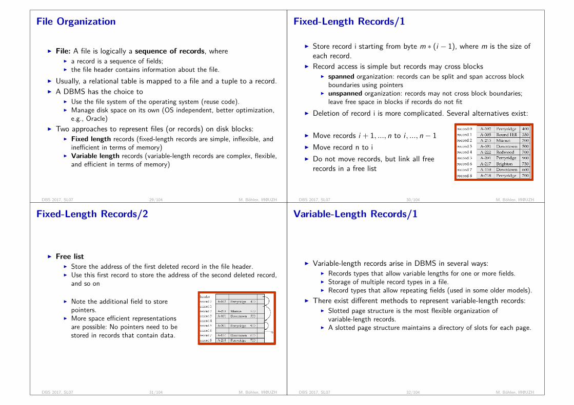
File Organization
I File: A file is logically a sequence of records, whereI a record is a sequence of fields;I the file header contains information about the file.
I Usually, a relational table is mapped to a file and a tuple to a record.I A DBMS has the choice to
I Use the file system of the operating system (reuse code).I Manage disk space on its own (OS independent, better optimization,
e.g., Oracle)I Two approaches to represent files (or records) on disk blocks:
I Fixed length records (fixed-length records are simple, inflexible, andinefficient in terms of memory)
I Variable length records (variable-length records are complex, flexible,and efficient in terms of memory)
DBS 2017, SL07 29/104 M. Böhlen, IfI@UZH
Fixed-Length Records/1
I Store record i starting from byte m ∗ (i − 1), where m is the size ofeach record.
I Record access is simple but records may cross blocksI spanned organization: records can be split and span accross block
boundaries using pointersI unspanned organization: records may not cross block boundaries;
leave free space in blocks if records do not fitI Deletion of record i is more complicated. Several alternatives exist:
I Move records i + 1, ..., n to i , ..., n − 1I Move record n to iI Do not move records, but link all free
records in a free list
DBS 2017, SL07 30/104 M. Böhlen, IfI@UZH
Fixed-Length Records/2
I Free listI Store the address of the first deleted record in the file header.I Use this first record to store the address of the second deleted record,
and so on
I Note the additional field to storepointers.
I More space efficient representationsare possible: No pointers need to bestored in records that contain data.
DBS 2017, SL07 31/104 M. Böhlen, IfI@UZH
Variable-Length Records/1
I Variable-length records arise in DBMS in several ways:I Records types that allow variable lengths for one or more fields.I Storage of multiple record types in a file.I Record types that allow repeating fields (used in some older models).
I There exist different methods to represent variable-length records:I Slotted page structure is the most flexible organization of
variable-length records.I A slotted page structure maintains a directory of slots for each page.
DBS 2017, SL07 32/104 M. Böhlen, IfI@UZH

Variable-Length Records/2
I Slotted page structureI Slotted page header contains:
I number of record entriesI end of free space in the blockI location and size of each record
I Records can be moved around in a page to keep them contiguous withno empty space between them; entry in the header must be updated.
I Pointers should not point directly to record - instead they shouldpoint to the entry for the record in header.
DBS 2017, SL07 33/104 M. Böhlen, IfI@UZH
Organization of Records in Files/1
There are different ways to logically organize records in a file (this iscalled the primary file organization):
I Heap file organization: A record can be placed anywhere in the filewhere there is space; there is no ordering in the file.
books unordered
I Sequential file organization: Store records in sequential orderbased on the value of the search key of each record.
books ordered byauthor
I Hash file organization: A hash function is computed on someattribute of each record; the result specifies in which block of thefile the record is placed.
books grouped by area (novels, cs, German lite-rature, ...)
I Generally, each relation is stored in a separate file.
DBS 2017, SL07 34/104 M. Böhlen, IfI@UZH
Organization of Records in Files/2
I Sequential file: The records in the file are ordered by a search key(one or more attributes)
I Records are chained together by pointersI Suitable for applications that require sequential processing of the
entire fileI To be efficient, records should also be stored physically in search key
order (or close to it).I Example: account(account-number,branch-name,balance)
DBS 2017, SL07 35/104 M. Böhlen, IfI@UZH
Organization of Records in Files/3
I It is difficult to maintain the physical order as records are insertedand deleted.
I Deletion: Store a deletion marker with each record; use pointer chainsto build a free list
I Insertion:I Locate the position where the record
is to be insertedI If there is free space insert thereI If no free space, insert the record in
an overflow blockI Need to reorganize the file from time
to time to restore (physical) sequentialorder
DBS 2017, SL07 36/104 M. Böhlen, IfI@UZH
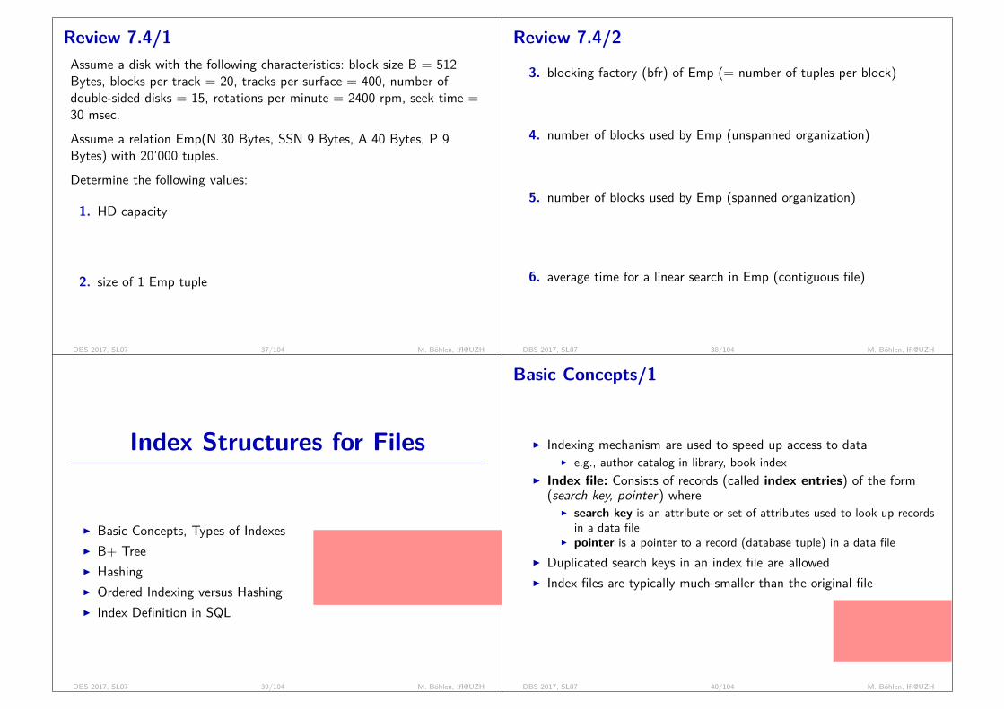
Review 7.4/1Assume a disk with the following characteristics: block size B = 512Bytes, blocks per track = 20, tracks per surface = 400, number ofdouble-sided disks = 15, rotations per minute = 2400 rpm, seek time =30 msec.Assume a relation Emp(N 30 Bytes, SSN 9 Bytes, A 40 Bytes, P 9Bytes) with 20’000 tuples.Determine the following values:
1. HD capacity
20 ∗ 512 ∗ 400 ∗ 2 ∗ 15 = 122.9MB
2. size of 1 Emp tuple
30 + 9 + 40 + 9 + 1 = 89Bytes (1 as, e.g., a deletion marker)
DBS 2017, SL07 37/104 M. Böhlen, IfI@UZH
Review 7.4/2
3. blocking factory (bfr) of Emp (= number of tuples per block)
bfr = bB/89c = 5tuples/block
4. number of blocks used by Emp (unspanned organization)
20′000/5 = 4000blocks
5. number of blocks used by Emp (spanned organization)
20′000 ∗ (89/(512− 4)) = 3505blocks (4 Bytes for pointer to nextblock)
6. average time for a linear search in Emp (contiguous file)
2000 ∗ btt + st + rd = 2.04sec (half of blocks on avg, btt=1msec,st=30msec, rd=12.5msec
DBS 2017, SL07 38/104 M. Böhlen, IfI@UZH
Index Structures for Files
I Basic Concepts, Types of IndexesI B+ TreeI HashingI Ordered Indexing versus HashingI Index Definition in SQL
size of dictionary/index (for, e.g., 10GBdata)?
size of index is 1 to 10 times the sizeof the data (i.e., 10-100GB in this case);variance is very large (e.g., Google)
DBS 2017, SL07 39/104 M. Böhlen, IfI@UZH
Basic Concepts/1
I Indexing mechanism are used to speed up access to dataI e.g., author catalog in library, book index
I Index file: Consists of records (called index entries) of the form(search key, pointer) where
I search key is an attribute or set of attributes used to look up recordsin a data file
I pointer is a pointer to a record (database tuple) in a data fileI Duplicated search keys in an index file are allowedI Index files are typically much smaller than the original file
library + indexphones + phone bookencyclopedia + tocdissertation + glossaryWWW + Google index)
DBS 2017, SL07 40/104 M. Böhlen, IfI@UZH
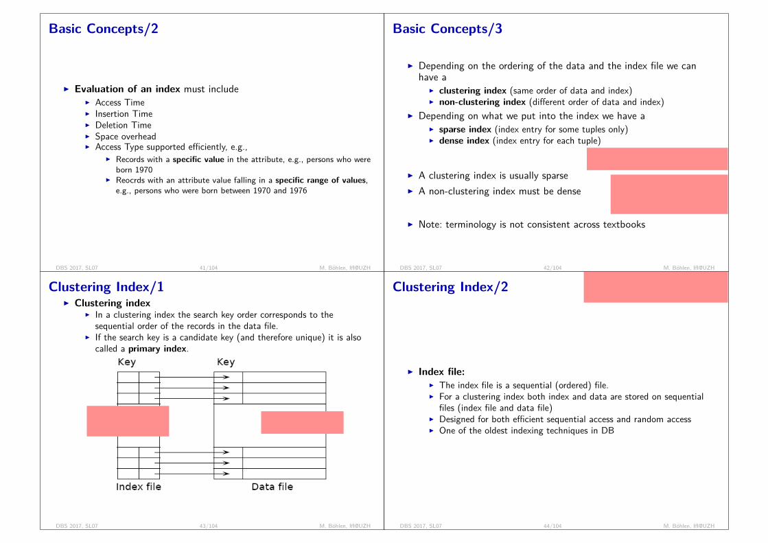
Basic Concepts/2
I Evaluation of an index must includeI Access TimeI Insertion TimeI Deletion TimeI Space overheadI Access Type supported efficiently, e.g.,
I Records with a specific value in the attribute, e.g., persons who wereborn 1970
I Reocrds with an attribute value falling in a specific range of values,e.g., persons who were born between 1970 and 1976
DBS 2017, SL07 41/104 M. Böhlen, IfI@UZH
Basic Concepts/3
I Depending on the ordering of the data and the index file we canhave a
I clustering index (same order of data and index)I non-clustering index (different order of data and index)
I Depending on what we put into the index we have aI sparse index (index entry for some tuples only)I dense index (index entry for each tuple)
I A clustering index is usually sparse
Duden, Lexikon, Wörterbuch (Ordnungder Daten = Ordnung Index)
I A non-clustering index must be dense
Glossar/Schlagwortverzeichnis,Telefonbuch (Ordnung derDaten is different from OrdnungIndex)
I Note: terminology is not consistent across textbooks
DBS 2017, SL07 42/104 M. Böhlen, IfI@UZH
Clustering Index/1I Clustering index
I In a clustering index the search key order corresponds to thesequential order of the records in the data file.
I If the search key is a candidate key (and therefore unique) it is alsocalled a primary index.
Schlagwortverzeichnisder Wörter (alphabe-tisch geordnet)
Lexikon (alphabetischgeordnet)
DBS 2017, SL07 43/104 M. Böhlen, IfI@UZH
Clustering Index/2
there can be at most one clustering (pri-mary) index! important decision (i.e.,how to order your data).
I Index file:I The index file is a sequential (ordered) file.I For a clustering index both index and data are stored on sequential
files (index file and data file)I Designed for both efficient sequential access and random accessI One of the oldest indexing techniques in DB
DBS 2017, SL07 44/104 M. Böhlen, IfI@UZH

Non-Clustering Indexes/1
Example: books ordered according toISBN and index ordered according to au-thor last name.
I Non-Clustering indexes are used to quickly find all records whosevalues in a certain field satisfy some condition.
I Example: Consider an account relation that is stored sequentially byaccount number
I Find all accounts in a particular branchI Find all accounts with a specified balance or range of balances
I The above query can only be answered by retrieving and checking allrecords (very inefficient).
I An additional (non-clustering) index is needed to answer suchqueries efficiently.
DBS 2017, SL07 45/104 M. Böhlen, IfI@UZH
Non-Clustering Indexes/2I Non-clustering index: Index whose search key specifies an orderdifferent from the sequential order of the file
I Non-clustering indexes are also called secondary indexes.I Non-clustering indexes must be dense, i.e., they must include an
index entry for every search key value and a pointer to every recordin the data file.
Autorenverzeichnis (al-phabetisch geordnet)
Library ordered accor-ding to ISBN)
DBS 2017, SL07 46/104 M. Böhlen, IfI@UZH
Non-Clustering Indexes/3I Two options for data pointers
I Duplicate index entries: an index record for every data recordI Buckets: An index record for each search key value; index record
points to a bucket that contains pointers to all the actual recordswith that particular search key value
I Example: Non-Clustering index on the balance field of the accountrelation using buckets
DBS 2017, SL07 47/104 M. Böhlen, IfI@UZH
Review 7.5I Relation R(A,B, ...) with 6M tuples.I Clustering index on A. Non-clustering index on B.I 200 index entries per block. 50 tuples per block.I Values of A and B are uniformly distributed in [0, 100M].I Use indexes to answer Q1 = σ[A > 75M](r) and Q2 = σ[B > 75M](r).
Determine the number of IOs. Interpret the result.
I 6M/200 = 30’000 index blocks.I 6M/50 = 120’000 data blocks.I Strategy:
1. find starting point (first block) with binary search2. scan index to the end3. for each entry fetch all tuples
I Q1 : log2(30′000) + 30′000/4 + 120′000/4 = 37’015 blocksI Q2 : log2(30′000) + 30′000/4 + 1.5M = 1’507’515 blocks
DBS 2017, SL07 48/104 M. Böhlen, IfI@UZH
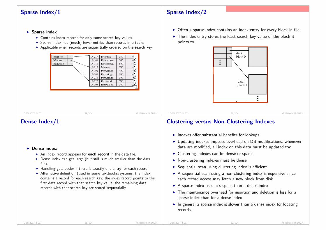
Sparse Index/1
I Sparse indexI Contains index records for only some search key values.I Sparse index has (much) fewer entries than records in a table.I Applicable when records are sequentially ordered on the search key
DBS 2017, SL07 49/104 M. Böhlen, IfI@UZH
Sparse Index/2
Dictionary: one entry per page (at the top of the page)
I Often a sparse index contains an index entry for every block in file.I The index entry stores the least search key value of the block it
points to.
DBS 2017, SL07 50/104 M. Böhlen, IfI@UZH
Dense Index/1
I Dense index:I An index record appears for each record in the data file.I Dense index can get large (but still is much smaller than the data
file).I Handling gets easier if there is exactly one entry for each record.I Alternative definition (used in some textbooks/systems: the index
contains a record for each search key; the index record points to thefirst data record with that search key value; the remaining datarecords with that search key are stored sequentially
DBS 2017, SL07 51/104 M. Böhlen, IfI@UZH
Clustering versus Non-Clustering Indexes
I Indexes offer substantial benefits for lookupsI Updating indexes imposes overhead on DB modifications: whenever
data are modified, all index on this data must be updated tooI Clustering indexes can be dense or sparseI Non-clustering indexes must be denseI Sequential scan using clustering index is efficientI A sequential scan using a non-clustering index is expensive since
each record access may fetch a new block from diskI A sparse index uses less space than a dense indexI The maintenance overhead for insertion and deletion is less for a
sparse index than for a dense indexI In general a sparse index is slower than a dense index for locating
records.
DBS 2017, SL07 52/104 M. Böhlen, IfI@UZH
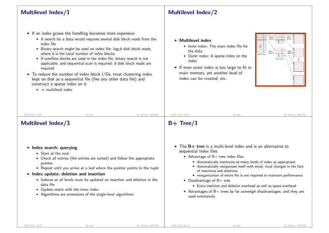
Multilevel Index/1
I If an index grows the handling becomes more expensiveI A search for a data record requires several disk block reads from the
index fileI Binary search might be used on index file: log2b disk block reads,
where b is the total number of index blocksI If overflow blocks are used in the index file, binary search is not
applicable, and sequential scan is required: b disk block reads arerequired
I To reduce the number of index block I/Os, treat clustering indexkept on disk as a sequential file (like any other data file) andconstruct a sparse index on it
I ⇒ multilevel index
DBS 2017, SL07 53/104 M. Böhlen, IfI@UZH
Multilevel Index/2
I Multilevel indexI Inner index: The main index file for
the dataI Outer index: A sparse index on the
indexI If even outer index is too large to fit in
main memory, yet another level ofindex can be created, etc.
DBS 2017, SL07 54/104 M. Böhlen, IfI@UZH
Multilevel Index/3
I Index search: queryingI Start at the rootI Check all entries (the entries are sorted) and follow the appropriate
pointerI Repeat until you arrive at a leaf where the pointer points to the tuple
I Index update: deletion and insertionI Indexes at all levels must be updated on insertion and deletion in the
data fileI Update starts with the inner indexI Algorithms are extensions of the single-level algorithms
DBS 2017, SL07 55/104 M. Böhlen, IfI@UZH
B+ Tree/1
I The B+ tree is a multi-level index and is an alternative tosequential index files
I Advantage of B+ tree index filesI Automatically maintains as many levels of index as appropriateI Automatically reorganizes itself with small, local changes in the face
of insertions and deletionsI reorganization of entire file is not required to maintain performance
I Disadvantage of B+ treeI Extra insertion and deletion overhead as well as space overhead
I Advantages of B+ trees by far outweigh disadvantages, and they areused extensively
DBS 2017, SL07 56/104 M. Böhlen, IfI@UZH
B+ Tree/2
I B+ tree: a rooted tree with the following propertiesP0 K1 P1 ... Km−1 Pm−1
P1 K1 ... Pm−1 Km−1 Pm
I Balanced tree, i.e., all paths from root to leaf are of the same length(at most dlogdm/2e(K )e for K search key values)
I A node contains up to m − 1 search key values and m pointers, andthe search key values within a node are sorted
I Nodes are between half and completely fullI Internal nodes have between dm/2e and m childrenI Leaf nodes have between d(m − 1)/2e and m - 1 search key valuesI Root node: If it is a leaf, it can have between 0 and m − 1 search
key values; otherwise, it has at least 2 children
DBS 2017, SL07 57/104 M. Böhlen, IfI@UZH
Terminology and Notation
I A pair (Pi ,Ki) in a leaf node is an entryI A pair (Ki ,Pi) in an internal (i.e., non-leaf) node is an entryI L[i ] denotes the value of the ith entry in node LI Data pointers are stored at leaf nodes onlyI Leaf nodes are linked together: the last pointer in a node points to
the next leaf node.
I Note that there are many small variations of B+ tree; textbooksdiffer; stick to approach described on these slides.
DBS 2017, SL07 58/104 M. Böhlen, IfI@UZH
B+ Tree Node Structure/1
P1 K1 P2 K2 ... Pm−1 Km−1 PmI Leaf nodesI K1, . . . ,Km−1 are the search key valuesI P1, ...,Pm−1 are pointers to records or buckets of records (for leaf
nodes)I The search keys in a node are ordered: K1 < K2 < K3 < ... < Km−1I Pi points to the database tuples with search keys X equal to KiI P1,. . . ,Pm−1 either point to a file record with search key value Ki
(unique) or to a bucket of pointers to file records with search keyvalue Ki (non-unique)
I Bucket structure is only needed if search key does not form a primarykey
I Pointer Pm points to next leaf node in search key order
DBS 2017, SL07 59/104 M. Böhlen, IfI@UZH
B+ Tree Node Structure/2
P0 K1 P1 K2 P2 ... Km−1 Pm−1I Internal nodesI Form a multi-level sparse index on the leaf nodesI P0, ...,Pm−1 are pointers to children (for non-leaf nodes)I Pi points to a subtree with search keys X such that Ki ≤ X < Ki+1
I P0 points to the subtree where all search key values are less than K1I For 1 ≤ i < m − 1: Pointer Pi points to the subtree where all search
key values are greater than or equal to Ki and less than Ki+1I Pointer Pm−1 points to the subtree where all search key values are
greater than or equal to Km−1
DBS 2017, SL07 60/104 M. Böhlen, IfI@UZH

Example of B+ Tree/1
I B+ tree for account file (m=5 pointers per node)I Leaf nodes: between 2 and 4 search key values (d(m − 1)/2e and
m − 1)I Non-leaf nodes other than root: between 3 and 5 children (d(m/2e
and m))I Root node: at least 2 children
Perryridge
Brighton Downtown Mianus Perryridge Redwood Round Hill
DBS 2017, SL07 61/104 M. Böhlen, IfI@UZH
Example of B+ Tree/2
I B+ tree for account file (m=3)I Leaf nodes: between 1 and 2 search key values (d(m − 1)/2e and
m − 1)I Non-leaf nodes other than root: between 2 and 3 children (d(m/2e
and m))I Root node: at least 2 children
Perryridge
Mianus Redwood
Brighton Downtown Mianus Perryridge Redwood Round Hill
DBS 2017, SL07 62/104 M. Böhlen, IfI@UZH
Observations about B+ Trees/1
I B+ tree for account fileI Since the inter-node connections are done by pointers, logically close
blocks need not be physically closeI gives flexibilityI increases times for seeks and latency
I The non-leaf levels of the B+ tree form a hierarchy of sparse indexes(= multilevel index on leaf nodes)
I The B+ tree contains a relatively small number of levelsI dlogdm/2e(K)e for K search key values in the file
DBS 2017, SL07 63/104 M. Böhlen, IfI@UZH
Observations about B+ Trees/2
I Search is efficient, since only a small number of index blocksneed to be read
I Compare to the log2(b) disk block reads for binary search insequential index files
I Typically the root node and perhaps the first level nodes are kept inmain memory, which further reduces the disk block reads.
I Insertions and deletions to the main file can be handledefficiently, as the index can be restructured in logarithmic time
DBS 2017, SL07 64/104 M. Böhlen, IfI@UZH
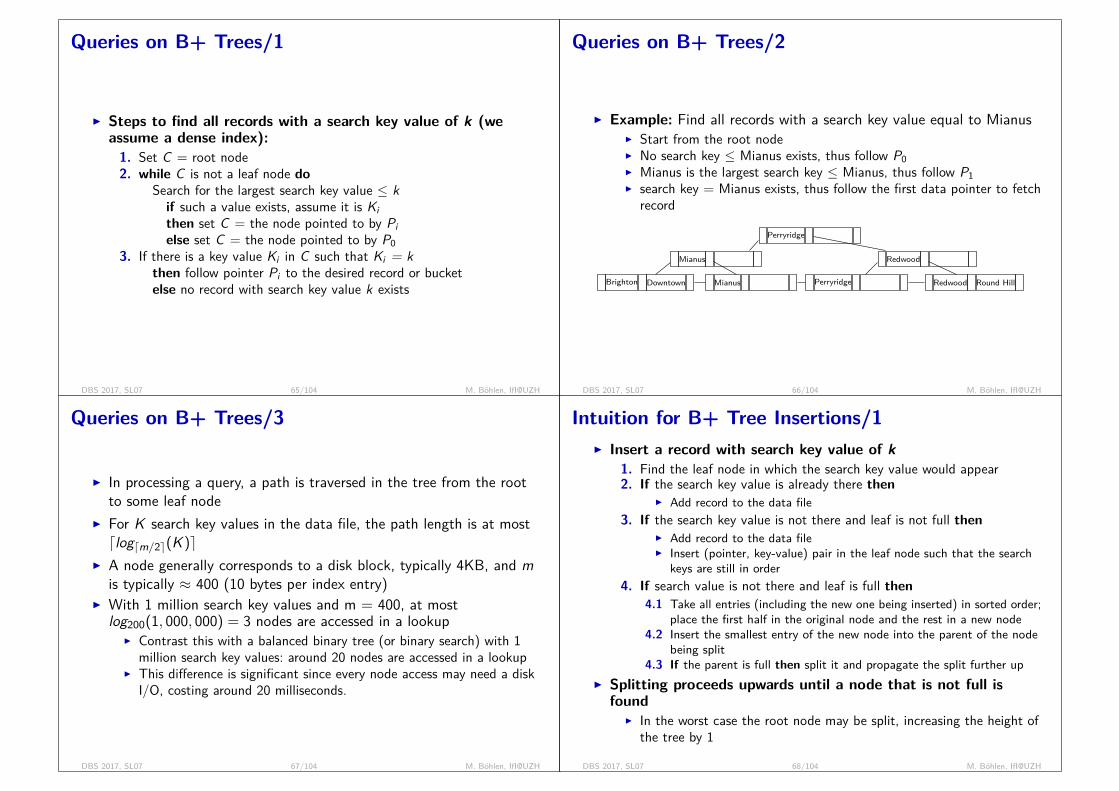
Queries on B+ Trees/1
I Steps to find all records with a search key value of k (weassume a dense index):1. Set C = root node2. while C is not a leaf node do
Search for the largest search key value ≤ kif such a value exists, assume it is Kithen set C = the node pointed to by Pielse set C = the node pointed to by P0
3. If there is a key value Ki in C such that Ki = kthen follow pointer Pi to the desired record or bucketelse no record with search key value k exists
DBS 2017, SL07 65/104 M. Böhlen, IfI@UZH
Queries on B+ Trees/2
I Example: Find all records with a search key value equal to MianusI Start from the root nodeI No search key ≤ Mianus exists, thus follow P0I Mianus is the largest search key ≤ Mianus, thus follow P1I search key = Mianus exists, thus follow the first data pointer to fetch
record
Perryridge
Mianus Redwood
Brighton Downtown Mianus Perryridge Redwood Round Hill
DBS 2017, SL07 66/104 M. Böhlen, IfI@UZH
Queries on B+ Trees/3
I In processing a query, a path is traversed in the tree from the rootto some leaf node
I For K search key values in the data file, the path length is at mostdlogdm/2e(K )e
I A node generally corresponds to a disk block, typically 4KB, and mis typically ≈ 400 (10 bytes per index entry)
I With 1 million search key values and m = 400, at mostlog200(1, 000, 000) = 3 nodes are accessed in a lookup
I Contrast this with a balanced binary tree (or binary search) with 1million search key values: around 20 nodes are accessed in a lookup
I This difference is significant since every node access may need a diskI/O, costing around 20 milliseconds.
DBS 2017, SL07 67/104 M. Böhlen, IfI@UZH
Intuition for B+ Tree Insertions/1I Insert a record with search key value of k
1. Find the leaf node in which the search key value would appear2. If the search key value is already there then
I Add record to the data file3. If the search key value is not there and leaf is not full then
I Add record to the data fileI Insert (pointer, key-value) pair in the leaf node such that the search
keys are still in order4. If search value is not there and leaf is full then
4.1 Take all entries (including the new one being inserted) in sorted order;place the first half in the original node and the rest in a new node
4.2 Insert the smallest entry of the new node into the parent of the nodebeing split
4.3 If the parent is full then split it and propagate the split further upI Splitting proceeds upwards until a node that is not full isfound
I In the worst case the root node may be split, increasing the height ofthe tree by 1
DBS 2017, SL07 68/104 M. Böhlen, IfI@UZH
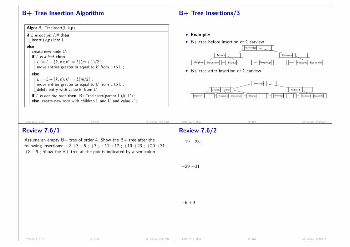
B+ Tree Insertion Algorithm
Algo: B+TreeInsert(L,k,p)if L is not yet full then
insert (k,p) into Lelse
create new node L’;if L is a leaf then
L := L + (k, p); k ′ := Ld(m + 1)/2e ;move entries greater or equal to k’ from L to L’;
elseL := L + (k, p); k ′ := Ldm/2e ;move entries greater or equal to k’ from L to L’;delete entry with value k’ from L’
if L is not the root then B+TreeInsert(parent(L),k’,L’) ;else create new root with children L and L’ and value k’ ;
DBS 2017, SL07 69/104 M. Böhlen, IfI@UZH
B+ Tree Insertions/3
I Example:I B+ tree before insertion of Clearview
Perryridge
Mianus Redwood
Brighton Downtown Mianus Perryridge Redwood Round Hill
I B+ tree after insertion of Clearview
Perryridge
Clearview Mianus Redwood
Brighton Clearview Downtown Mianus Perryridge Redwood Round Hill
DBS 2017, SL07 70/104 M. Böhlen, IfI@UZH
Review 7.6/1Assume an empty B+ tree of order 4. Show the B+ tree after thefollowing insertions: +2 +3 +5 ; +7 ; +11 +17 ; +19 +23 ; +29 +31 ;+8 +9 ; Show the B+ tree at the points indicated by a semicolon.
+2 +3 +5:2 3 5
+7:5
2 3 5 7+11 +17:
5 11
2 3 5 7 11 17
DBS 2017, SL07 71/104 M. Böhlen, IfI@UZH
Review 7.6/2+19 +23:
5 11 19
2 3 5 7 11 17 19 23
+29 +31
11
5
2 3 5 7
19 29
11 17 19 23 29 31
+8 +9
11
5 8
2 3 5 7 8 9
19 29
11 17 19 23 29 31
DBS 2017, SL07 72/104 M. Böhlen, IfI@UZH

Intuition for B+ Tree Deletions/1
I Deletion of a record with search key k1. Find leaf node with (pointer, key-value) entry; remove entry2. If the node has too few entries due to the removal, and the entries in
the node and a sibling fit into a single node thenI Coalesce siblings, i.e., insert all search key values in the two nodes
into a single node (the one on the left if it exists; the right otherwise)and delete the other node
I Delete the entry in parent node that is between the two nodes byapplying the deletion procedure recursively
3. If the node has too few entries due to the removal, and the entries inthe node and a sibling do not fit into a single node then
I Redistribute the pointers between the node and a sibling such thatboth have more than the minimum number of entries
I Update the corresponding search key value in the parent of the nodeI Node deletions may cascade upwards till a node with dm/2e or more
pointers is found. If the root node has only one pointer afterdeletion, it is deleted and the child becomes the root.
DBS 2017, SL07 73/104 M. Böhlen, IfI@UZH
B+ Tree Deletion AlgorithmAlgo: B+TreeDelete(L,k,p)delete (p,k) from L;if L is root with one child then root := child;else if L has too few entries then
L’ is previous sibling of L [next if there is no previous] ;k’ is value in parent that is between L and L’;if entries L and L’ fit on one page then
if L is leaf then move entries from L to L’;else move k’ and all entries from L to L’;B+TreeDelete(parent(L),k’,L)
elseif L is leaf then
move last [first] entry of L’ to L;replace k’ in parent(L) by value of first entry in L [L’];
elsemove [first] last entry of L’ to L;replace k’ in parent(L) by value of first entry of L [L’];replace value of first entry in L [L’] by k’;
DBS 2017, SL07 74/104 M. Böhlen, IfI@UZH
B+ Tree Deletions/3
I Example: Before deleting Downtown
Perryridgs
Downtown Mianus Redwood
Brighton Clearview Downtown Mianus Perryridge Redwood Round Hill
I After deleting DowntownPerryridgs
Mianus Redwood
Brighton Clearview Mianus Perryridge Redwood Round Hill
I The removal of the leaf node containing Downtown do not result inits parent having too little pointers. So the cascaded deletionsstopped with the deleted leaf node’s parent.
DBS 2017, SL07 75/104 M. Böhlen, IfI@UZH
B+ Tree Deletions/4I Example: Before deleting Perryridge
Perryridge
Mianus Redwood
Brighton Clearview Mianus Perryridge Redwood Round Hill
I After deleting PerryridgeMianus Perryridge
Brighton Clearview Mianus Redwood Round Hill
I Node with Perryridge becomes underfull and is merged with itssibling.
I As a result Perryridge node’s parent becomes underfull, and iscoalesced with its sibling (and an entry is deleted from theirparent).
I Root node then has only one child and is deleted.
DBS 2017, SL07 76/104 M. Böhlen, IfI@UZH
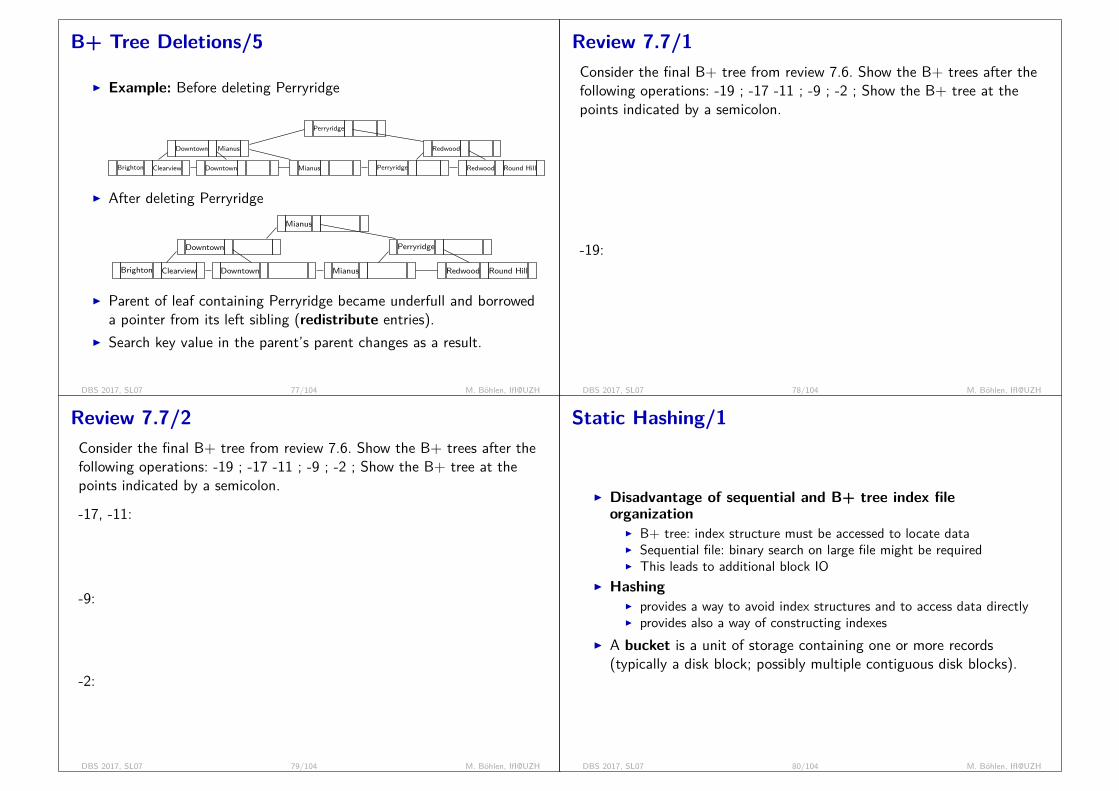
B+ Tree Deletions/5
I Example: Before deleting Perryridge
Perryridge
Downtown Mianus Redwood
Brighton Clearview Downtown Mianus Perryridge Redwood Round Hill
I After deleting PerryridgeMianus
Downtown Perryridge
Brighton Clearview Downtown Mianus Redwood Round Hill
I Parent of leaf containing Perryridge became underfull and borroweda pointer from its left sibling (redistribute entries).
I Search key value in the parent’s parent changes as a result.
DBS 2017, SL07 77/104 M. Böhlen, IfI@UZH
Review 7.7/1Consider the final B+ tree from review 7.6. Show the B+ trees after thefollowing operations: -19 ; -17 -11 ; -9 ; -2 ; Show the B+ tree at thepoints indicated by a semicolon.
11
5 8
2 3 5 7 8 9
19 29
11 17 19 23 29 31
-19:
11
5 8
2 3 5 7 8 9
29
11 17 23 29 31
DBS 2017, SL07 78/104 M. Böhlen, IfI@UZH
Review 7.7/2Consider the final B+ tree from review 7.6. Show the B+ trees after thefollowing operations: -19 ; -17 -11 ; -9 ; -2 ; Show the B+ tree at thepoints indicated by a semicolon.
-17, -11:
5 8 11
2 3 5 7 8 9 23 29 31
-9:
5 11
2 3 5 7 8 23 29 31
-2:
7 11
3 5 7 8 23 29 31
DBS 2017, SL07 79/104 M. Böhlen, IfI@UZH
Static Hashing/1
I Disadvantage of sequential and B+ tree index fileorganization
I B+ tree: index structure must be accessed to locate dataI Sequential file: binary search on large file might be requiredI This leads to additional block IO
I HashingI provides a way to avoid index structures and to access data directlyI provides also a way of constructing indexes
I A bucket is a unit of storage containing one or more records(typically a disk block; possibly multiple contiguous disk blocks).
DBS 2017, SL07 80/104 M. Böhlen, IfI@UZH
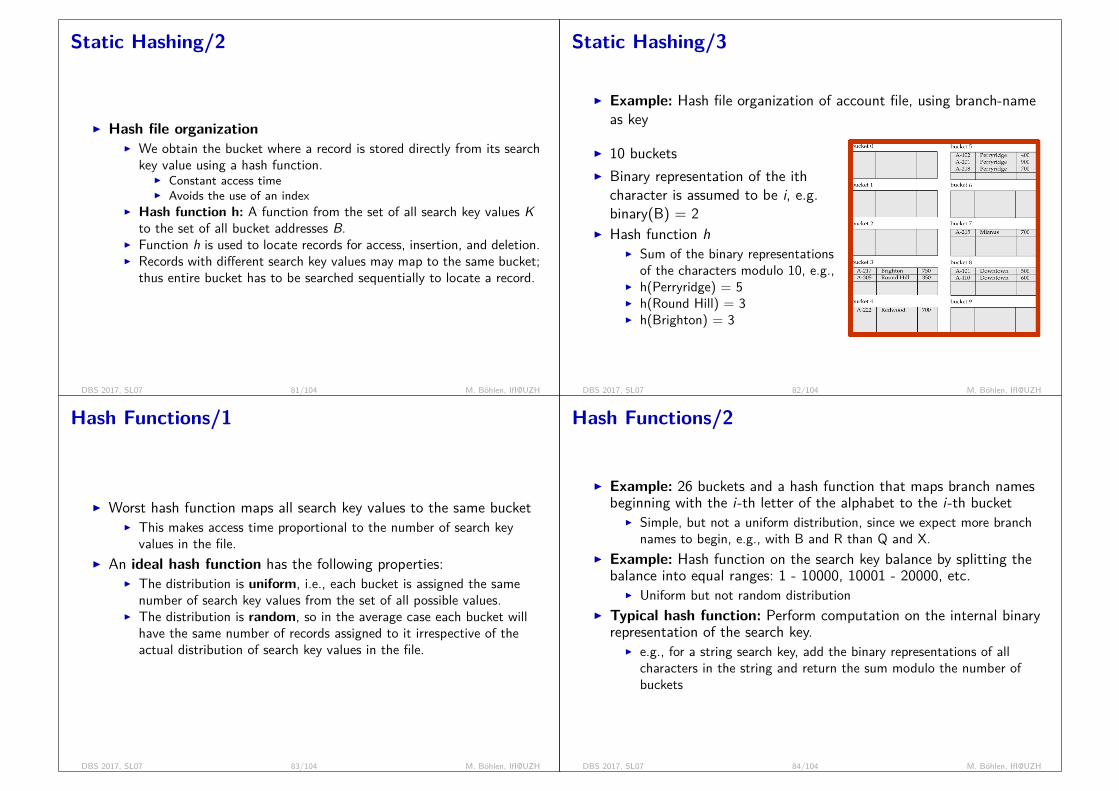
Static Hashing/2
I Hash file organizationI We obtain the bucket where a record is stored directly from its search
key value using a hash function.I Constant access timeI Avoids the use of an index
I Hash function h: A function from the set of all search key values Kto the set of all bucket addresses B.
I Function h is used to locate records for access, insertion, and deletion.I Records with different search key values may map to the same bucket;
thus entire bucket has to be searched sequentially to locate a record.
DBS 2017, SL07 81/104 M. Böhlen, IfI@UZH
Static Hashing/3
I Example: Hash file organization of account file, using branch-nameas key
I 10 bucketsI Binary representation of the ith
character is assumed to be i, e.g.binary(B) = 2
I Hash function hI Sum of the binary representations
of the characters modulo 10, e.g.,I h(Perryridge) = 5I h(Round Hill) = 3I h(Brighton) = 3
DBS 2017, SL07 82/104 M. Böhlen, IfI@UZH
Hash Functions/1
I Worst hash function maps all search key values to the same bucketI This makes access time proportional to the number of search key
values in the file.I An ideal hash function has the following properties:
I The distribution is uniform, i.e., each bucket is assigned the samenumber of search key values from the set of all possible values.
I The distribution is random, so in the average case each bucket willhave the same number of records assigned to it irrespective of theactual distribution of search key values in the file.
DBS 2017, SL07 83/104 M. Böhlen, IfI@UZH
Hash Functions/2
I Example: 26 buckets and a hash function that maps branch namesbeginning with the i-th letter of the alphabet to the i-th bucket
I Simple, but not a uniform distribution, since we expect more branchnames to begin, e.g., with B and R than Q and X.
I Example: Hash function on the search key balance by splitting thebalance into equal ranges: 1 - 10000, 10001 - 20000, etc.
I Uniform but not random distributionI Typical hash function: Perform computation on the internal binary
representation of the search key.I e.g., for a string search key, add the binary representations of all
characters in the string and return the sum modulo the number ofbuckets
DBS 2017, SL07 84/104 M. Böhlen, IfI@UZH
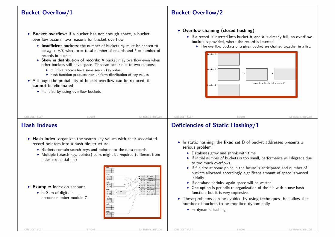
Bucket Overflow/1
I Bucket overflow: If a bucket has not enough space, a bucketoverflow occurs; two reasons for bucket overflow
I Insufficient buckets: the number of buckets nB must be chosen tobe nB > n/f, where n = total number of records and f = number ofrecords in bucket
I Skew in distribution of records: A bucket may overflow even whenother buckets still have space. This can occur due to two reasons:
I multiple records have same search key valueI hash function produces non-uniform distribution of key values
I Although the probability of bucket overflow can be reduced, itcannot be eliminated!
I Handled by using overflow buckets
DBS 2017, SL07 85/104 M. Böhlen, IfI@UZH
Bucket Overflow/2
I Overflow chaining (closed hashing)I If a record is inserted into bucket b, and b is already full, an overflowbucket is provided, where the record is inserted
I The overflow buckets of a given bucket are chained together in a list.
DBS 2017, SL07 86/104 M. Böhlen, IfI@UZH
Hash Indexes
I Hash index: organizes the search key values with their associatedrecord pointers into a hash file structure.
I Buckets contain search keys and pointers to the data recordsI Multiple (search key, pointer)-pairs might be required (different from
index-sequential file)
I Example: Index on accountI h: Sum of digits in
account-number modulo 7
DBS 2017, SL07 87/104 M. Böhlen, IfI@UZH
Deficiencies of Static Hashing/1
I In static hashing, the fixed set B of bucket addresses presents aserious problem
I Databases grow and shrink with timeI If initial number of buckets is too small, performance will degrade due
to too much overflows.I If file size at some point in the future is anticipated and number of
buckets allocated accordingly, significant amount of space is wastedinitially.
I If database shrinks, again space will be wastedI One option is periodic re-organization of the file with a new hash
function, but it is very expensive.I These problems can be avoided by using techniques that allow the
number of buckets to be modified dynamicallyI ⇒ dynamic hashing
DBS 2017, SL07 88/104 M. Böhlen, IfI@UZH
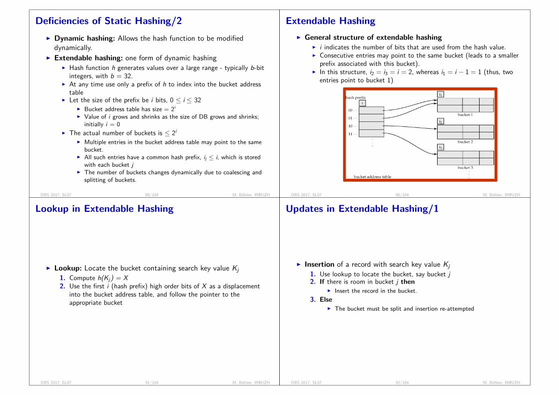
Deficiencies of Static Hashing/2I Dynamic hashing: Allows the hash function to be modified
dynamically.I Extendable hashing: one form of dynamic hashing
I Hash function h generates values over a large range - typically b-bitintegers, with b = 32.
I At any time use only a prefix of h to index into the bucket addresstable
I Let the size of the prefix be i bits, 0 ≤ i ≤ 32I Bucket address table has size = 2i
I Value of i grows and shrinks as the size of DB grows and shrinks;initially i = 0
I The actual number of buckets is ≤ 2i
I Multiple entries in the bucket address table may point to the samebucket.
I All such entries have a common hash prefix, ij ≤ i, which is storedwith each bucket j
I The number of buckets changes dynamically due to coalescing andsplitting of buckets.
DBS 2017, SL07 89/104 M. Böhlen, IfI@UZH
Extendable HashingI General structure of extendable hashing
I i indicates the number of bits that are used from the hash value.I Consecutive entries may point to the same bucket (leads to a smaller
prefix associated with this bucket).I In this structure, i2 = i3 = i = 2, whereas i1 = i − 1 = 1 (thus, two
entries point to bucket 1)
DBS 2017, SL07 90/104 M. Böhlen, IfI@UZH
Lookup in Extendable Hashing
I Lookup: Locate the bucket containing search key value Kj1. Compute h(Kj) = X2. Use the first i (hash prefix) high order bits of X as a displacement
into the bucket address table, and follow the pointer to theappropriate bucket
DBS 2017, SL07 91/104 M. Böhlen, IfI@UZH
Updates in Extendable Hashing/1
I Insertion of a record with search key value Kj1. Use lookup to locate the bucket, say bucket j2. If there is room in bucket j then
I Insert the record in the bucket.3. Else
I The bucket must be split and insertion re-attempted
DBS 2017, SL07 92/104 M. Böhlen, IfI@UZH
Updates in Extendable Hashing/2
I Split a bucket j when inserting search key value KjI If i > ij (more than one pointer to bucket j) then
I Allocate a new bucket z, and set ij and iz to the old ij + 1.I Update bucket address table entries that point to j according to
prefix (some will now point to z)I Remove and reinsert each record in bucket j.I Recompute new bucket for Kj and insert record in the bucket (further
splitting is required if the bucket is still full).I If i = ij (only one pointer to bucket j) then
I Increment i and double the size of the bucket address table.I Replace each entry in the table by two entries that point to the same
bucket.I Recompute new bucket address table entry for Kj
I Overflow buckets needed instead of splitting (or in addition) in somecases, e.g., too many records with same hash value.
DBS 2017, SL07 93/104 M. Böhlen, IfI@UZH
Updates in Extendable Hashing/3
I Deletion of a key value K1. Locate K in its bucket and remove it (search key from bucket and
record from the file).2. The bucket itself can be removed if it becomes empty (with
appropriate updates to the bucket address table).3. Coalescing of buckets can be done (can coalesce only with a buddy
bucket having same value of ij and same ij -1 prefix, if it is present).4. Decreasing bucket address table size is also possible.
I Note: Decreasing bucket address table size is an expensiveoperation and should be done only if number of buckets becomesmuch smaller than the size of the table
DBS 2017, SL07 94/104 M. Böhlen, IfI@UZH
Review 7.8/1Consider the following hash function: h(Brighton) = 0010, h(Downtown)= 1010, h(Mianus) = 1100, h(Perryridge) = 1111, h(Redwood) = 0011.Assume a bucket size of two and extendable hashing with an addresstable size of 1. Show the hash table after the following modifications:
I insert 1 Brighton and 2 Downtown recordsI insert 1 Mianus recordI insert 1 Redwood recordI insert 3 Perryridge records
DBS 2017, SL07 95/104 M. Böhlen, IfI@UZH
Review 7.8/2
0 0 1
1Brighton
1DowntownDowntown
2
1Brighton
2DowntownDowntown
2Mianus
2
1BrightonRedwood
2DowntownDowntown
2Mianus
3
1BrightonRedwood
2DowntownDowntown
3Mianus
3PerryridgePerryride
3Perryridge
DBS 2017, SL07 96/104 M. Böhlen, IfI@UZH
Extendable Hashing: Discussion
I Benefits of extendable hashingI Hash performance does not degrade with growth of fileI Minimal space overheadI No buckets are reserved for future growth, but are allocated
dynamically.I Disadvantages of extendable hashing
I Extra level of indirection to find desired recordI Bucket address table may itself become very big (larger than
memory)I Need a tree structure to locate desired record in the structure
I Changing size of bucket address table is expensive
DBS 2017, SL07 97/104 M. Böhlen, IfI@UZH
Ordered Indexing versus Hashing
I Cost of periodic re-organizationI Hashmaps (e.g., Google’s sparse and dense hash maps) do not
provide constant insert/lookup time because of reorganizationI Relative frequency of insertions and deletions
I B+ trees are better than hashing if there are many database updatesI Is it desirable to optimize average access time at the expense of
worst-case access time?I Hashing has a better average time but no worst case guarantees
I Expected type of queries:I Hashing is generally better at retrieving records having a specified
value of the key.I If range queries are common, ordered indexes are to be preferred
I There is no ordering in hash organization, and hence there is nonotion of "next record in sort order".
DBS 2017, SL07 98/104 M. Böhlen, IfI@UZH
Berkeley DB
DBS 2017, SL07 99/104 M. Böhlen, IfI@UZH
Index Definition in SQL
I SQL-92 does not define syntax for indexes because these are notconsidered part of the logical data model
I All DBMSs (must) provide support for indexesI Create an index:
create index <IdxName> on <RelName> (<AttrList>)E.g,: create index BrNaIdx on branch (branch-name)
I Create unique index to indirectly specify and enforce the conditionthat the search key is a candidate key.
I Not really required if SQL unique integrity constraint is supportedI To drop an index: drop index <index-name>
E.g,: drop index BrNaIdx
DBS 2017, SL07 100/104 M. Böhlen, IfI@UZH
Indexes in PostgreSQL
I CREATE [UNIQUE] INDEX name ON table_name”(” col [DESC] { "," col [DESC] } ”)” [. . . ]
I CREATE INDEX MjIdx ON enroll (Major)
I CREATE INDEX MjIdx ON enroll USING HASH (Major)
I CREATE INDEX MjMnIdx ON Enroll (Major, Minor)
I Properties of indexes:I Indexes are automatically maintained as data are inserted, deleted,
and updated.I Indexes slow down database modification statements.I Creating an index can take a long time.
DBS 2017, SL07 101/104 M. Böhlen, IfI@UZH
Indexes in OracleI B+ tree indexes in Oracle
CREATE [UNIQUE] INDEX name ON table_name”(” col [DESC] { "," col [DESC] } ”)” [pctfree n] [. . . ]
I pct_free specifies how many percent of a index page are left unfilledinitially (dafult to 10%)
I In index definitions UNIQUE should not be used because it is a logicalconcept.
I Oracle creates a B+ Tree index for each unique (and primary key)declaration.
CREATE TABLE BOOKISBN INTEGER, Author VARCHAR2(30), . . .);
CREATE INDEX book_auth ON book(Author);
I Creating a hash-partitioned global index:CREATE INDEX CustLNameIX ON customers(LName)GLOBAL PARTITION BY HASH (LName)PARTITIONS 4;
DBS 2017, SL07 102/104 M. Böhlen, IfI@UZH
Summary/1
I Physical storage mediaI storage hierarchy: cache, RAM, flash, disk, optical disk, tape, ...
I Accessing the storageI block-based access:
I know characteristics of disksI compute number of IOsI compute execution time
I buffer managerI Organization of files
I fixed-length record, variable-length recordI heap file (unordered), sequential file (ordered), hash file
DBS 2017, SL07 103/104 M. Böhlen, IfI@UZH
Summary/2
I Definition of and differences between index typesI clustering and non-clustering indexI dense and sparse index
I B+ treeI universal database access structure; also for range predicatesI definition (node, leaf, non-leaf, entry)I insertion and deletion
I HashingI static and extendable hashingI no index structure needed for primary index (hash function gives
record location directly)I good for equality predicates (used heavily in applications)
I Index definition in SQL
DBS 2017, SL07 104/104 M. Böhlen, IfI@UZH

Database SystemsSpring 2017
Query Processing and QueryOptimization
SL08I Query Processing
I Sorting, PartitioningI Selection, Join
I Query OptimizationI Cost estimationI Rewriting of relational algebra expressionsI Rule- and cost-based query optimization
Reviews: 15 22 31 32 38 44 56 63 73
DBS 2017, SL08 1/82 M. Böhlen, IfI@UZH
Literature and Acknowledgments
Reading List for SL08:I Database Systems, Chapter 18, Sixth Edition, Ramez Elmasri and
Shamkant B. Navathe, Pearson Education, 2010.
These slides were developed by:I Michael Böhlen, University of Zürich, SwitzerlandI Johann Gamper, Free University of Bozen-Bolzano, Italy
The slides are based on the following text books and associated material:I Database Systems, Sixth Edition, Ramez Elmasri and Shamkant B.
Navathe, Pearson Education, 2010.I A. Silberschatz, H. Korth, and S. Sudarshan: Database System
Concepts, McGraw Hill, 2006.
DBS 2017, SL08 2/82 M. Böhlen, IfI@UZH
PostgreSQL Example/1
DBS 2017, SL08 3/82 M. Böhlen, IfI@UZH
PostgreSQL Example/2
DBS 2017, SL08 4/82 M. Böhlen, IfI@UZH
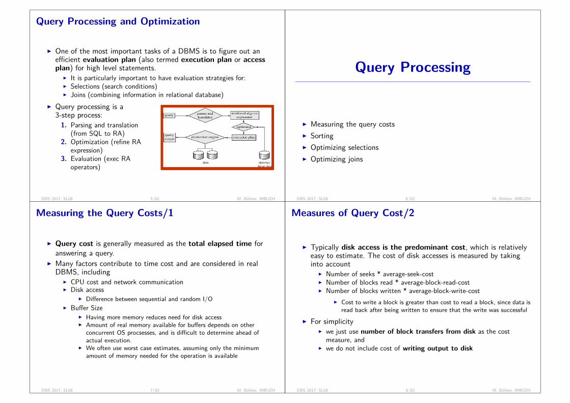
Query Processing and Optimization
I One of the most important tasks of a DBMS is to figure out anefficient evaluation plan (also termed execution plan or accessplan) for high level statements.
I It is particularly important to have evaluation strategies for:I Selections (search conditions)I Joins (combining information in relational database)
I Query processing is a3-step process:1. Parsing and translation
(from SQL to RA)2. Optimization (refine RA
expression)3. Evaluation (exec RA
operators)
DBS 2017, SL08 5/82 M. Böhlen, IfI@UZH
Query Processing
I Measuring the query costsI SortingI Optimizing selectionsI Optimizing joins
DBS 2017, SL08 6/82 M. Böhlen, IfI@UZH
Measuring the Query Costs/1
I Query cost is generally measured as the total elapsed time foranswering a query.
I Many factors contribute to time cost and are considered in realDBMS, including
I CPU cost and network communicationI Disk access
I Difference between sequential and random I/OI Buffer Size
I Having more memory reduces need for disk accessI Amount of real memory available for buffers depends on other
concurrent OS procsesses, and is difficult to determine ahead ofactual execution.
I We often use worst case estimates, assuming only the minimumamount of memory needed for the operation is available
DBS 2017, SL08 7/82 M. Böhlen, IfI@UZH
Measures of Query Cost/2
I Typically disk access is the predominant cost, which is relativelyeasy to estimate. The cost of disk accesses is measured by takinginto account
I Number of seeks * average-seek-costI Number of blocks read * average-block-read-costI Number of blocks written * average-block-write-cost
I Cost to write a block is greater than cost to read a block, since data isread back after being written to ensure that the write was successful
I For simplicityI we just use number of block transfers from disk as the cost
measure, andI we do not include cost of writing output to disk
DBS 2017, SL08 8/82 M. Böhlen, IfI@UZH
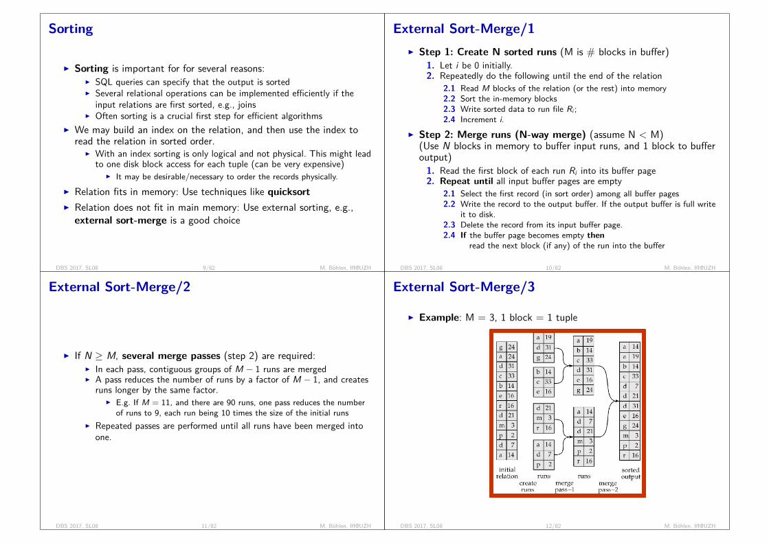
Sorting
I Sorting is important for for several reasons:I SQL queries can specify that the output is sortedI Several relational operations can be implemented efficiently if the
input relations are first sorted, e.g., joinsI Often sorting is a crucial first step for efficient algorithms
I We may build an index on the relation, and then use the index toread the relation in sorted order.
I With an index sorting is only logical and not physical. This might leadto one disk block access for each tuple (can be very expensive)
I It may be desirable/necessary to order the records physically.I Relation fits in memory: Use techniques like quicksortI Relation does not fit in main memory: Use external sorting, e.g.,external sort-merge is a good choice
DBS 2017, SL08 9/82 M. Böhlen, IfI@UZH
External Sort-Merge/1I Step 1: Create N sorted runs (M is # blocks in buffer)
1. Let i be 0 initially.2. Repeatedly do the following until the end of the relation
2.1 Read M blocks of the relation (or the rest) into memory2.2 Sort the in-memory blocks2.3 Write sorted data to run file Ri ;2.4 Increment i.
I Step 2: Merge runs (N-way merge) (assume N < M)(Use N blocks in memory to buffer input runs, and 1 block to bufferoutput)1. Read the first block of each run Ri into its buffer page2. Repeat until all input buffer pages are empty
2.1 Select the first record (in sort order) among all buffer pages2.2 Write the record to the output buffer. If the output buffer is full write
it to disk.2.3 Delete the record from its input buffer page.2.4 If the buffer page becomes empty then
read the next block (if any) of the run into the buffer
DBS 2017, SL08 10/82 M. Böhlen, IfI@UZH
External Sort-Merge/2
I If N ≥ M, several merge passes (step 2) are required:I In each pass, contiguous groups of M − 1 runs are mergedI A pass reduces the number of runs by a factor of M − 1, and creates
runs longer by the same factor.I E.g. If M = 11, and there are 90 runs, one pass reduces the number
of runs to 9, each run being 10 times the size of the initial runsI Repeated passes are performed until all runs have been merged into
one.
DBS 2017, SL08 11/82 M. Böhlen, IfI@UZH
External Sort-Merge/3
I Example: M = 3, 1 block = 1 tuple
DBS 2017, SL08 12/82 M. Böhlen, IfI@UZH

External Sort-Merge/4
I Cost analysisI br = number of blocks in rI Initial number of runs: br/MI Total number of merge passes required: dlogM−1(br/M)e
I The number of runs decreases by a factor of M-1 in each merge passI Disk accesses for initial run creation and in each pass is 2br
I Exception: For final pass there is no write costI Thus total number of disk accesses for external sorting:
Cost = br (2 dlogM−1(br/M) e + 1)
I Example: Cost analysis of previous exampleI 12 ( 2 * 2 + 1) = 60 disk block transfers
DBS 2017, SL08 13/82 M. Böhlen, IfI@UZH
Selection Evaluation Strategies/1
I The selection operator:I select * from r where θI σθ(r)
is used to retrieve those records that satisfy the selection condition
I The strategy/algorithm for the evaluation of the selection operatordepends
I on the type of the selection conditionI on the available index structures
DBS 2017, SL08 14/82 M. Böhlen, IfI@UZH
Review 8.1Assume a B+ tree index on (BrName, BrCity). What would be the bestway to evaluate the query:
σBrCity<′Brighton′ ∧ Assets<5000 ∧ BrName=′Downtown′(branch)
1. use index to locate 1st tuple with BrName = ’Downtown’2. retrieve successive data tuples as long as BrCity is less than
’Brighton’3. for each tuple we check if Asset < 5000 (only such tuples are
returned)index:BrName BrCity ptrCS Oerlikon p1CS Uster p1CS ZH p1UBS Aarau p1UBS Bern p1
DBS 2017, SL08 15/82 M. Böhlen, IfI@UZH
Selection Evaluation Strategies/2
Types of selection conditions:
I Equality queries: σa=v (r)
I Range queries: σa≤v (r) or σa≥v (r)I Can be implemented by using
I linear file scanI binary searchI using indices
I Conjunctive selection: σθ1∧θ2···∧θn(r)
I Disjunctive selection: σθ1∨θ2···∨θn(r)
DBS 2017, SL08 16/82 M. Böhlen, IfI@UZH
Selection Evaluation Strategies/3
Basic search methods for selection operator:
I File scanI Class of search algorithms that read the file line by line to locate
and retrieve records that fulfill a selection condition, i.e., σθ(r)I Lowest-level operator to access data
I Index scanI Class of search algorithms that use an indexI Assume B+ tree index and equality conditions, i.e., σa=v (r)
DBS 2017, SL08 17/82 M. Böhlen, IfI@UZH
Selection Evaluation Strategies/4
I A1 Linear search: Scan each file block and test all records to seewhether they satisfy the selection condition.
I Fairly expensive, but always applicable (regardless of indexes,ordering, selection condition, etc)
I Fetching a contiguous range of blocks from disk has been optimizedby disk manufacturers and is cheap in terms of seek time androtational delay (pre-fetching)
I Cost estimate (br = number of blocks in file):I Worst case: Cost = brI If the selection is on a key attribute: Average cost = br/2 (stop
when finding record)
DBS 2017, SL08 18/82 M. Böhlen, IfI@UZH
Selection Evaluation Strategies/5
I A2 Binary search: Apply binary search to locate records thatsatisfy selection condition.
I Only applicable ifI the blocks of a relation are stored contiguously (very rare), andI the selection condition is a comparison on the attribute on which the
file is orderedI Cost estimate for σA=v (r):
I dlog2(br )e — cost of locating the first tuple by a binary search on theblocks
I Plus number of blocks containing records that satisfy selectioncondition
DBS 2017, SL08 19/82 M. Böhlen, IfI@UZH
Selection Evaluation Strategies/6
I A3 Primary index + equality on candidate keyI Retrieve a single record that satisfies the equality conditionI Cost = HTi + 1 (height of B+ tree + 1 data block)
I A4 Primary index + equality on non-candidate keyI Retrieve multiple records, where records are on consecutive blocksI Cost = HTi + # blocks with records with given search key
I A5 Secondary index + equality on search-keyI Retrieve a single record if the search-key is a candidate key
I Cost = HTi + 1I Retrieve multiple records if search-key is not a candidate key
I Cost = HTi + # buckets with search-key value + # retrieved recordsI Can be very expensive, since each record may be on a different blockI Linear file scan may be cheaper if many records have to be fetched
DBS 2017, SL08 20/82 M. Böhlen, IfI@UZH
Selection Evaluation Strategies/7
I A6 Primary index on A + non-equality conditionI σA≥v : Use index to find first tuple ≥ v ; then scan relation sequentiallyI σa≤v : Scan relation sequentially until first tuple > v ; do not use index.
I A7 Secondary index on A + non-equality conditionI σA≥v : Use index to find first index entry ≥ v ; scan index sequentially
from there, to find pointers to records.I σA≤v : Scan leaf pages of index finding record pointers until first entry> v
I Requires in the worst case one I/O for each record; linear file scanmay be cheaper if many records are to be fetched
DBS 2017, SL08 21/82 M. Böhlen, IfI@UZH
Review 8.2Consider relations r1(A,B,C), r2(C ,D,E ), r3(E ,F ) with keysunderlined and cardinalities |r1| = 1000, |r2| = 1500, |r3| = 750.
I Estimate the size of r1 1 r2 1 r3I Give an efficient strategy for computing the result and compute its
cost
I |r1 1 r2| ≤ 1000I |(r1 1 r2) 1 r3| ≤ 1000I (primary) index on r2.C and r3.E (create if necessary)for each tuple t in r do
look up 1 tuple in r2 using index on r2.C;look up 1 tuple in r3 using index on r3.E
I cost of joins: |r1| ∗ (HTr2.C + HTr2.C ) (independent of size ofr2 and r3)
I cost index creation:O(br1∗logM(br1/M))+O(br2∗logM(br2/M))+O(br2)+O(br3)
DBS 2017, SL08 22/82 M. Böhlen, IfI@UZH
Join Evaluation Strategies
I There exist several different algorithms for the evaluation of joinoperations:
I Nested loop joinI Block nested loop joinI Indexed nested loop joinI Merge joinI Hash join
I Choice based on cost estimateI Examples use the following relations:
I customer = (CustName, CustStreet, CustCity)I Number of records: nc = 10′000I Number of blocks: bc = 400
I depositor = (CustName, AccNumber)I Number of records: nd = 5′000I Number of blocks: bd = 100
DBS 2017, SL08 23/82 M. Böhlen, IfI@UZH
Nested Loop Join/1
I Compute the theta join: r 1θ sfor each tuple tr in r do
for each tuple ts in s doif pair (tr ,t − s) satisfies join condition θ then
add tr ◦ ts to result
I r is called the outer relation, s the inner relation of the join.I Always applicable. Requires no indices and can be used with any
kind of join condition.I Expensive since it examines every pair of tuples.
DBS 2017, SL08 24/82 M. Böhlen, IfI@UZH
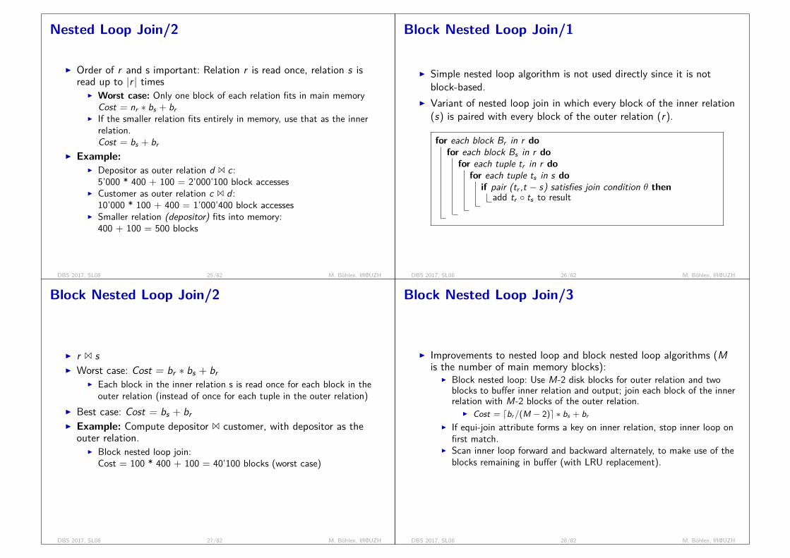
Nested Loop Join/2
I Order of r and s important: Relation r is read once, relation s isread up to |r | times
I Worst case: Only one block of each relation fits in main memoryCost = nr ∗ bs + br
I If the smaller relation fits entirely in memory, use that as the innerrelation.Cost = bs + br
I Example:I Depositor as outer relation d 1 c:
5’000 * 400 + 100 = 2’000’100 block accessesI Customer as outer relation c 1 d :
10’000 * 100 + 400 = 1’000’400 block accessesI Smaller relation (depositor) fits into memory:
400 + 100 = 500 blocks
DBS 2017, SL08 25/82 M. Böhlen, IfI@UZH
Block Nested Loop Join/1
I Simple nested loop algorithm is not used directly since it is notblock-based.
I Variant of nested loop join in which every block of the inner relation(s) is paired with every block of the outer relation (r).
for each block Br in r dofor each block Bs in r do
for each tuple tr in r dofor each tuple ts in s do
if pair (tr ,t − s) satisfies join condition θ thenadd tr ◦ ts to result
DBS 2017, SL08 26/82 M. Böhlen, IfI@UZH
Block Nested Loop Join/2
I r 1 sI Worst case: Cost = br ∗ bs + br
I Each block in the inner relation s is read once for each block in theouter relation (instead of once for each tuple in the outer relation)
I Best case: Cost = bs + brI Example: Compute depositor 1 customer, with depositor as the
outer relation.I Block nested loop join:
Cost = 100 * 400 + 100 = 40’100 blocks (worst case)
DBS 2017, SL08 27/82 M. Böhlen, IfI@UZH
Block Nested Loop Join/3
I Improvements to nested loop and block nested loop algorithms (Mis the number of main memory blocks):
I Block nested loop: Use M-2 disk blocks for outer relation and twoblocks to buffer inner relation and output; join each block of the innerrelation with M-2 blocks of the outer relation.
I Cost = dbr/(M − 2)e ∗ bs + br
I If equi-join attribute forms a key on inner relation, stop inner loop onfirst match.
I Scan inner loop forward and backward alternately, to make use of theblocks remaining in buffer (with LRU replacement).
DBS 2017, SL08 28/82 M. Böhlen, IfI@UZH
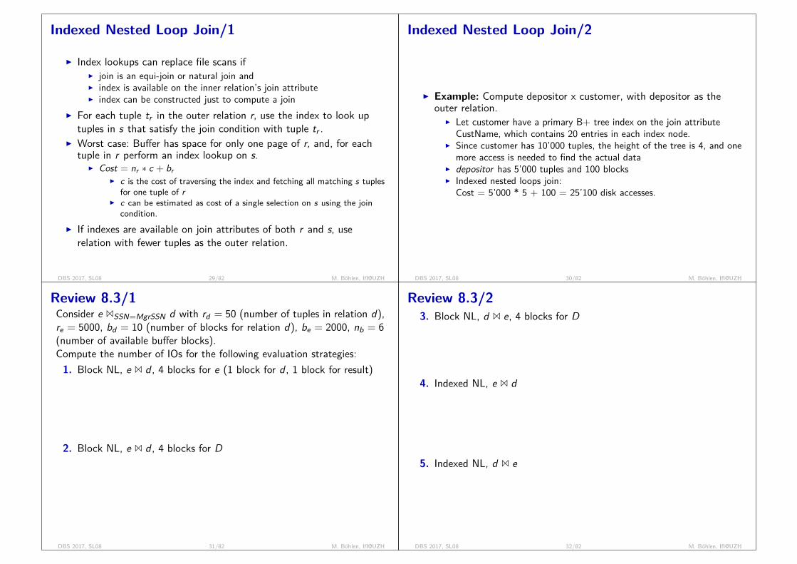
Indexed Nested Loop Join/1
I Index lookups can replace file scans ifI join is an equi-join or natural join andI index is available on the inner relation’s join attributeI index can be constructed just to compute a join
I For each tuple tr in the outer relation r, use the index to look uptuples in s that satisfy the join condition with tuple tr .
I Worst case: Buffer has space for only one page of r, and, for eachtuple in r perform an index lookup on s.
I Cost = nr ∗ c + brI c is the cost of traversing the index and fetching all matching s tuples
for one tuple of rI c can be estimated as cost of a single selection on s using the join
condition.I If indexes are available on join attributes of both r and s, use
relation with fewer tuples as the outer relation.
DBS 2017, SL08 29/82 M. Böhlen, IfI@UZH
Indexed Nested Loop Join/2
I Example: Compute depositor x customer, with depositor as theouter relation.
I Let customer have a primary B+ tree index on the join attributeCustName, which contains 20 entries in each index node.
I Since customer has 10’000 tuples, the height of the tree is 4, and onemore access is needed to find the actual data
I depositor has 5’000 tuples and 100 blocksI Indexed nested loops join:
Cost = 5’000 * 5 + 100 = 25’100 disk accesses.
DBS 2017, SL08 30/82 M. Böhlen, IfI@UZH
Review 8.3/1Consider e 1SSN=MgrSSN d with rd = 50 (number of tuples in relation d),re = 5000, bd = 10 (number of blocks for relation d), be = 2000, nb = 6(number of available buffer blocks).Compute the number of IOs for the following evaluation strategies:1. Block NL, e 1 d , 4 blocks for e (1 block for d , 1 block for result)
dbe/4e ∗ bd + be = 7′000
2. Block NL, e 1 d , 4 blocks for D
be ∗ bd + be = 22′000
DBS 2017, SL08 31/82 M. Böhlen, IfI@UZH
Review 8.3/23. Block NL, d 1 e, 4 blocks for D
dbd/4e ∗ be + bd = 6′010
4. Indexed NL, e 1 d
we assume a B+ index on d.MgrSSN of height 4be + ne(4 + 1) = 17′000
5. Indexed NL, d 1 e
bd + nd(4 + 1) = 260
DBS 2017, SL08 32/82 M. Böhlen, IfI@UZH

Merge Join/1
I Basic idea of merge join: Use two pointers pr and ps that areinitialized to the first tuple in r and s and move in a synchronizedway through the sorted relations.
I Algorithm1. Sort both relations on their
join attributes (if not alreadysorted on the join attribute).
2. Scan r and s in sort orderand return matching tuples.
3. Move the tuple pointer of therelation that is less faradvanced in sort order (morecomplicated if the joinattributes are not unique -every pair with same value onjoin attribute must bematched).
DBS 2017, SL08 33/82 M. Böhlen, IfI@UZH
Merge Join/2
I Applicable for equi-joins and natural joins onlyI If all tuples for any given value of the join attributes fit in memory
I One file scan of r and s is enoughI Cost = br + bs (+ the cost of sorting if relations are not sorted)
I Otherwise, a block nested loop join must be performed between thetuples with the same attributes
I If the relation are not sorted appropriately we first have to sortthem. The combined operator is called a sort-merge join.
DBS 2017, SL08 34/82 M. Böhlen, IfI@UZH
Hash Join/1
partition books on subject; partition 0 =cs, partition 1 = psy, partition 2 = eco
I Applicable for equi-joins and natural joins only.I Partition tuples of r and s using the same hash function h, which
maps the values of the join attributes to the set 0, 1, ..., nI Partitions of r-tuples: r0, r1, ..., rn
I All tr ε r with h(tr [JoinAttrs]) = iare put in ri
I Partitions of s-tuples: s0, s1, .., snI All ts ε s with h(ts [JoinAttrs]) = i
are put in si
I r -tuples in ri need only to be comparedwith s-tuples in si
I an r -tuples and s-tuples that satisfy the join condition have the samehash value i, and are mapped to ri and si , respectively.
DBS 2017, SL08 35/82 M. Böhlen, IfI@UZH
Hash Join/2
1st hash functions: partition books based on category(cs, psy, eco, ...); 2nd hash function must partition onsomething different than category
I Algorithm for the hash join of r and s1. Partition the relation s using hash function h. (When partitioning a
relation, one block of memory is reserved as the output buffer foreach partition.)
2. Partition r similarly.3. For each i :
3.1 Load si into memory and build an in-memory hash index on it usingthe join attribute. This hash index uses a different hash function thanthe earlier one h.
3.2 Read the tuples in ri from the disk (block by block). For each tuple trprobe (locate) each matching tuple ts in si using the in-memory hashindex. Output the concatenation of their attributes as result tuple.
I Relation s is called the build input and r is called the probe input.
DBS 2017, SL08 36/82 M. Böhlen, IfI@UZH
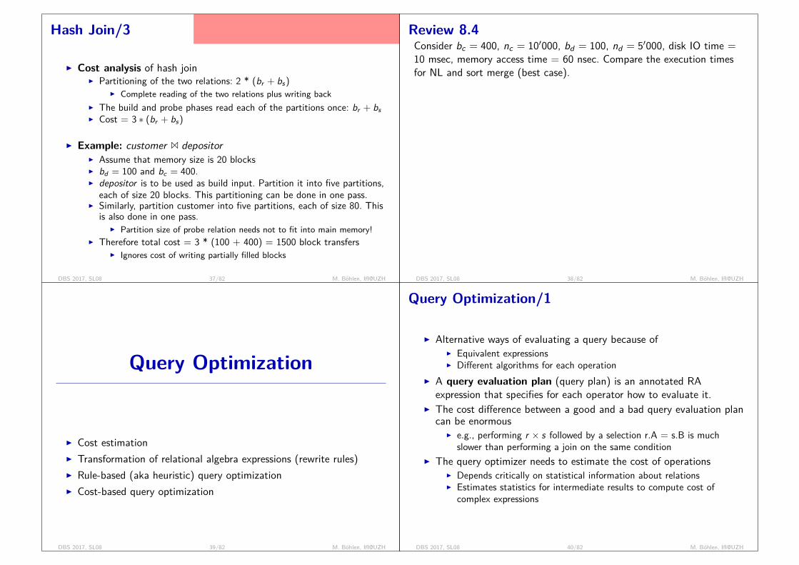
Hash Join/3
PostgreSQL uses hash join if build relation fits into me-mory; uses external sort merge otherwise; implementationrestriction
I Cost analysis of hash joinI Partitioning of the two relations: 2 * (br + bs)
I Complete reading of the two relations plus writing backI The build and probe phases read each of the partitions once: br + bsI Cost = 3 ∗ (br + bs)
I Example: customer 1 depositorI Assume that memory size is 20 blocksI bd = 100 and bc = 400.I depositor is to be used as build input. Partition it into five partitions,
each of size 20 blocks. This partitioning can be done in one pass.I Similarly, partition customer into five partitions, each of size 80. This
is also done in one pass.I Partition size of probe relation needs not to fit into main memory!
I Therefore total cost = 3 * (100 + 400) = 1500 block transfersI Ignores cost of writing partially filled blocks
DBS 2017, SL08 37/82 M. Böhlen, IfI@UZH
Review 8.4Consider bc = 400, nc = 10′000, bd = 100, nd = 5′000, disk IO time =10 msec, memory access time = 60 nsec. Compare the execution timesfor NL and sort merge (best case).
I # of IOs = bc + bd for both cases (best case = enoughmemory, relations already sorted)
I # of tuple comparisons in memoryI NL = nc ∗ ndI SM = nc + nd (unique attribute values)
I exact time NL:10 ∗ (bc + bd) + 60 ∗ 10−6(nc ∗ nd) = 5msec + 3msec = 8msec
I exact time SM:10∗(bc +bd)+60∗10−6(nc +nd) = 5msec+0.9msec = 5.9msec
I often IO time >> MEM time (and MEM is omitted forcomplexity)
I sometime MEM can become relevant (CPU versus IO bound)
DBS 2017, SL08 38/82 M. Böhlen, IfI@UZH
Query Optimization
I Cost estimationI Transformation of relational algebra expressions (rewrite rules)I Rule-based (aka heuristic) query optimizationI Cost-based query optimization
DBS 2017, SL08 39/82 M. Böhlen, IfI@UZH
Query Optimization/1
I Alternative ways of evaluating a query because ofI Equivalent expressionsI Different algorithms for each operation
I A query evaluation plan (query plan) is an annotated RAexpression that specifies for each operator how to evaluate it.
I The cost difference between a good and a bad query evaluation plancan be enormous
I e.g., performing r × s followed by a selection r.A = s.B is muchslower than performing a join on the same condition
I The query optimizer needs to estimate the cost of operationsI Depends critically on statistical information about relationsI Estimates statistics for intermediate results to compute cost of
complex expressions
DBS 2017, SL08 40/82 M. Böhlen, IfI@UZH

Query Optimization/2
I Step 1: Parsing and translationI Translate the query into its internal form (query tree)I The query tree corresponds to a relational algebra (RA) expressionI Each RA expression can be written as a tree where the algebra
operator is the root and the argument relations are the children.I Example:
I SQL query: select balance from account where balance < 2500I RA expression: σbalance<2500(πbalance(account))I Tree:
σbalance<2500|
πbalance|
account
DBS 2017, SL08 41/82 M. Böhlen, IfI@UZH
Query Optimization/3
I Step 2: OptimizationI An RA expression may have many (semantically) equivalent
expressionsI The following two RA expressions are equivalent:
I σbalance<2500(πbalance(account))I πbalance(σbalance<2500(account))
I Each RA operation can be evaluated using one of several differentalgorithms.
I Thus, an RA expression can be evaluated in many ways.
DBS 2017, SL08 42/82 M. Böhlen, IfI@UZH
Query Optimization/4
I Step 2: OptimizationI Evaluation plan: Annotated RA expression that specifies for each
operator detailed instructions on how to evaluate it.I use index on balance to find
accounts with balance < 2500I can perform complete relation
scan and discard accounts withbalance ≥ 2500
πbalance|σbalance<2500; use index 1|account
I Goal of query optimization: Among all equivalent evaluation planschoose the one with lowest cost.
I Cost is estimated using statistical information from the databasecatalog, e.g., number of tuples in each relation, size of tuples, etc.
I Step 3: EvaluationI The query-execution engine takes an evaluation plan, executes that
plan, and returns the answers.
DBS 2017, SL08 43/82 M. Böhlen, IfI@UZH
Review 8.5Display the trees that correspond to the following algebra expressions:
I RA1 = πA(R1 1 σX=Y (R2 1 πB,C (R3− R4) 1 R5))I RA2 = πA(R1) ∪ σX>5(R2)
∪
πA σX>5
R3 R4
πA
1
r1 σX=Y
1
1 r5
r2 πB,C
−
r3 r4
DBS 2017, SL08 44/82 M. Böhlen, IfI@UZH
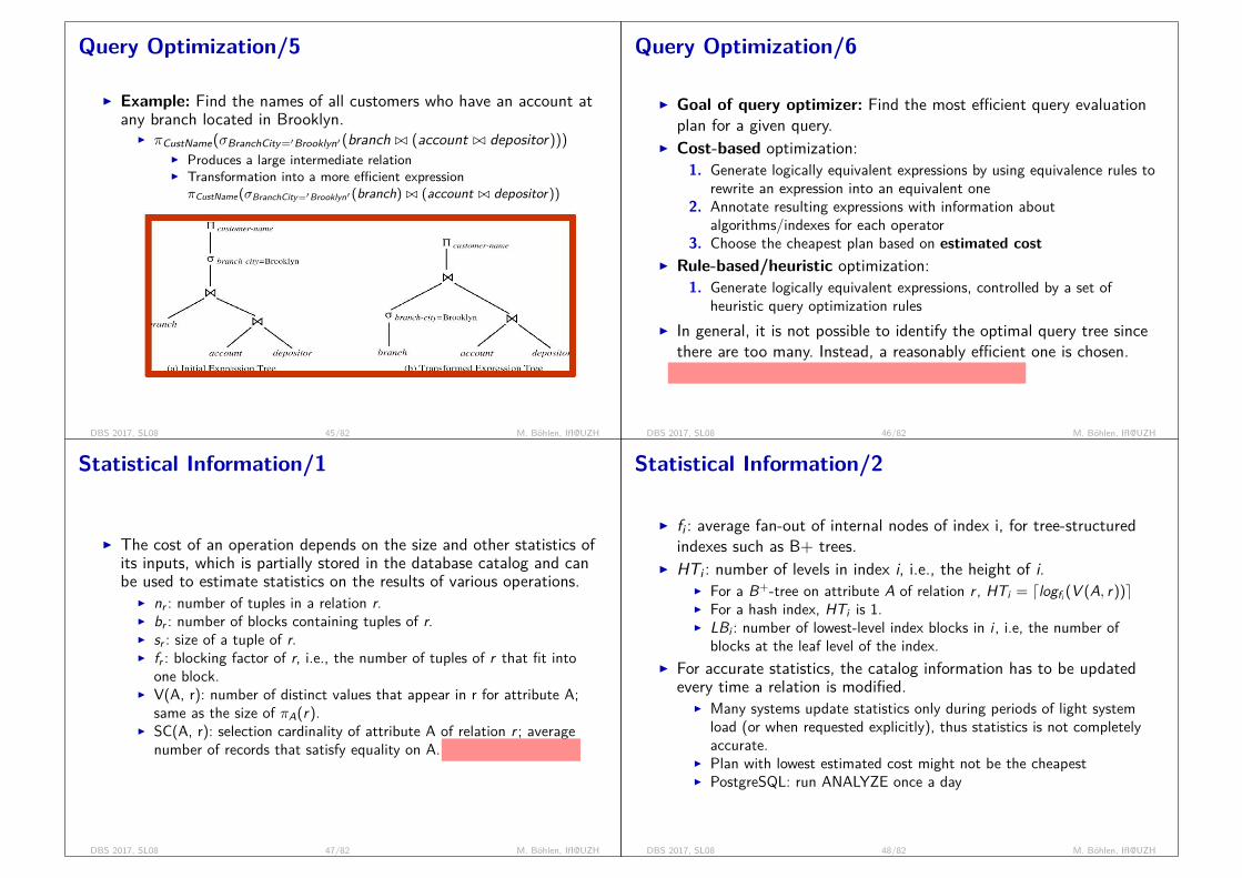
Query Optimization/5
I Example: Find the names of all customers who have an account atany branch located in Brooklyn.
I πCustName(σBranchCity=′Brooklyn′(branch ./ (account ./ depositor)))I Produces a large intermediate relationI Transformation into a more efficient expressionπCustName(σBranchCity=′Brooklyn′ (branch) ./ (account ./ depositor))
DBS 2017, SL08 45/82 M. Böhlen, IfI@UZH
Query Optimization/6
I Goal of query optimizer: Find the most efficient query evaluationplan for a given query.
I Cost-based optimization:1. Generate logically equivalent expressions by using equivalence rules to
rewrite an expression into an equivalent one2. Annotate resulting expressions with information about
algorithms/indexes for each operator3. Choose the cheapest plan based on estimated cost
I Rule-based/heuristic optimization:1. Generate logically equivalent expressions, controlled by a set of
heuristic query optimization rulesI In general, it is not possible to identify the optimal query tree since
there are too many. Instead, a reasonably efficient one is chosen.
how many? r1 1 ... 1 rn. all permutations. exponentially many!
DBS 2017, SL08 46/82 M. Böhlen, IfI@UZH
Statistical Information/1
I The cost of an operation depends on the size and other statistics ofits inputs, which is partially stored in the database catalog and canbe used to estimate statistics on the results of various operations.
I nr : number of tuples in a relation r.I br : number of blocks containing tuples of r.I sr : size of a tuple of r.I fr : blocking factor of r, i.e., the number of tuples of r that fit into
one block.I V(A, r): number of distinct values that appear in r for attribute A;
same as the size of πA(r).I SC(A, r): selection cardinality of attribute A of relation r ; average
number of records that satisfy equality on A.
SC(A, r) = nr/V (A, r)
DBS 2017, SL08 47/82 M. Böhlen, IfI@UZH
Statistical Information/2
I fi : average fan-out of internal nodes of index i, for tree-structuredindexes such as B+ trees.
I HTi : number of levels in index i, i.e., the height of i.I For a B+-tree on attribute A of relation r , HTi = dlogfi (V (A, r))eI For a hash index, HTi is 1.I LBi : number of lowest-level index blocks in i , i.e, the number of
blocks at the leaf level of the index.I For accurate statistics, the catalog information has to be updated
every time a relation is modified.I Many systems update statistics only during periods of light system
load (or when requested explicitly), thus statistics is not completelyaccurate.
I Plan with lowest estimated cost might not be the cheapestI PostgreSQL: run ANALYZE once a day
DBS 2017, SL08 48/82 M. Böhlen, IfI@UZH
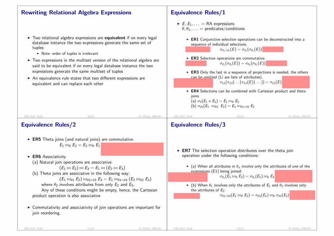
Rewriting Relational Algebra Expressions
I Two relational algebra expressions are equivalent if on every legaldatabase instance the two expressions generate the same set oftuples
I Note: order of tuples is irrelevantI Two expressions in the multiset version of the relational algebra are
said to be equivalent if on every legal database instance the twoexpressions generate the same multiset of tuples
I An equivalence rule states that two different expressions areequivalent and can replace each other
DBS 2017, SL08 49/82 M. Böhlen, IfI@UZH
Equivalence Rules/1I E ,E1, . . . = RA expressionsθ, θ1, . . . = predicates/conditions
I ER1 Conjunctive selection operations can be deconstructed into asequence of individual selections.
no good index
σθ1∧θ2(E ) = σθ1(σθ2(E ))
index for θ2
I ER2 Selection operations are commutative.
index for θ2
σθ1(σθ2(E )) = σθ2(σθ1(E ))
index for θ1
I ER3 Only the last in a sequence of projections is needed, the otherscan be omitted (Li are lists of attributes).
drop columns as early aspossible
πL1(πL2(. . . (πLn(E )) . . . )) = πL1(E )
drop many co-lumns in one ta-ble scan
I ER4 Selections can be combined with Cartesian product and thetajoins(a) σθ(E1 x E2) = E1 ./θ E2(b) σθ1(E1 ./θ2 E2) = E1 ./θ1∧θ2 E2
DBS 2017, SL08 50/82 M. Böhlen, IfI@UZH
Equivalence Rules/2
I ER5 Theta joins (and natural joins) are commutative.E1 ./θ E2 = E2 ./θ E1
inner relation small: either hash join whe-re build = inner relation or NL join whereinner relation in memory
I ER6 Associativity(a) Natural join operations are associative:
(E1 ./ E2) ./ E3 = E1 ./ (E2 ./ E3)(b) Theta joins are associative in the following way:
(E1 ./θ1 E2) ./θ2∧θ3 E3 = E1 ./θ1∧θ3 (E2 ./θ2 E3)where θ2 involves attributes from only E2 and E3.Any of these conditions might be empty, hence, the Cartesian
product operation is also associative
I Commutativity and associativity of join operations are important forjoin reordering.
DBS 2017, SL08 51/82 M. Böhlen, IfI@UZH
Equivalence Rules/3
I ER7 The selection operation distributes over the theta joinoperation under the following conditions:
I (a) When all attributes in θo involve only the attributes of one of theexpressions (E1) being joined:
θo has poor selectivity,Bal > 100, Lang = Engl
σθo (E1 ./θ E2) = σθo (E1) ./θ E2
θo has high selectivity,Bal > 1Billion, Lang =Danish
I (b) When θ1 involves only the attributes of E1 and θ2 involves onlythe attributes of E2:
poor selectivity
σθ1∧θ2(E1 ./θ E2) = σθ1(E1) ./θ σθ2(E2)
high selectivityof θ1, θ2
DBS 2017, SL08 52/82 M. Böhlen, IfI@UZH

Equivalence Rules/4
I ER8 The projection operation distributes over the theta joinoperation as follows:
I Let L1 and L2 be sets of attributes from E1 and E2, respectively.
I (a) if θ involves only attributes from L1 ∪ L2:πL1∪L2(E1 1θ E2) = πL1(E1) 1θ πL2(E2)
I (b) Consider a join E1 1θ E2.I Let L3 be attributes of E1 that are involved in join condition θ, but
are not in L1 ∪ L2, andI Let L4 be attributes of E2 that are involved in join condition θ, but
are not in L1 ∪ L2, andπL1∪L2(E1 1θ E2) = πL1∪L2(πL1∪L3(E1) 1θ πL2∪L4(E2))
DBS 2017, SL08 53/82 M. Böhlen, IfI@UZH
Equivalence Rules/5
A
B
C
I ER9 The set operations union and intersection are commutativeE1 ∪ E2 = E2 ∪ E1E1 ∩ E2 = E2 ∩ E1
Set difference is not commutative
I ER10 Set union and intersection are associative.(E1 ∪ E2) ∪ E3 = E1 ∪ (E2 ∪ E3)(E1 ∩ E2) ∩ E3 = E1 ∩ (E2 ∩ E3)
DBS 2017, SL08 54/82 M. Böhlen, IfI@UZH
Equivalence Rules/6
I ER11 The selection operation distributes over ∪,∩ and −.σθ(E1 − E2) = σθ(E1)− σθ(E2)σθ(E1 ∪ E2) = σθ(E1) ∪ σθ(E2)σθ(E1 ∩ E2) = σθ(E1) ∩ σθ(E2)
Also σθ(E1 − E2) = σθ(E1)− E2and similarly for ∩ in place of −, but not for ∪
I ER12 The projection operation distributes over unionπL(E1 ∪ E2) = πL(E ) ∪ πL(E2)
DBS 2017, SL08 55/82 M. Böhlen, IfI@UZH
Review 8.6Determine the equivalences that hold. Give counterexamples for the falseones.1. σθ(XϑF (A)) = XϑF (σθ(A)), attr(θ) ⊆ attr(X )
2. πX (A− B) = πX (A)− πX (B)
3. A d|><| (B d|><|C) = (A d|><|B) d|><|C
4. A ∩ B = A ∪ B − (A− B)− (B − A)
DBS 2017, SL08 56/82 M. Böhlen, IfI@UZH
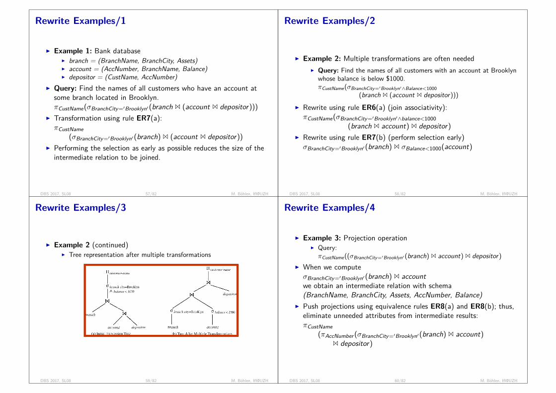
Rewrite Examples/1
I Example 1: Bank databaseI branch = (BranchName, BranchCity, Assets)I account = (AccNumber, BranchName, Balance)I depositor = (CustName, AccNumber)
I Query: Find the names of all customers who have an account atsome branch located in Brooklyn.πCustName(σBranchCity=′Brooklyn′(branch 1 (account 1 depositor)))
I Transformation using rule ER7(a):πCustName
(σBranchCity=′Brooklyn′(branch) 1 (account 1 depositor))I Performing the selection as early as possible reduces the size of the
intermediate relation to be joined.
DBS 2017, SL08 57/82 M. Böhlen, IfI@UZH
Rewrite Examples/2
I Example 2: Multiple transformations are often neededI Query: Find the names of all customers with an account at Brooklyn
whose balance is below $1000.πCustName(σBranchCity=′Brooklyn′∧Balance<1000
(branch 1 (account 1 depositor)))I Rewrite using rule ER6(a) (join associativity):πCustName(σBranchCity=′Brooklyn′∧balance<1000
(branch 1 account) 1 depositor)I Rewrite using rule ER7(b) (perform selection early)σBranchCity=′Brooklyn′(branch) 1 σBalance<1000(account)
DBS 2017, SL08 58/82 M. Böhlen, IfI@UZH
Rewrite Examples/3
I Example 2 (continued)I Tree representation after multiple transformations
DBS 2017, SL08 59/82 M. Böhlen, IfI@UZH
Rewrite Examples/4
I Example 3: Projection operationI Query:πCustName((σBranchCity=′Brooklyn′(branch) 1 account) 1 depositor)
I When we computeσBranchCity=′Brooklyn′(branch) 1 accountwe obtain an intermediate relation with schema(BranchName, BranchCity, Assets, AccNumber, Balance)
I Push projections using equivalence rules ER8(a) and ER8(b); thus,eliminate unneeded attributes from intermediate results:πCustName
(πAccNumber (σBranchCity=′Brooklyn′(branch) 1 account)1 depositor)
DBS 2017, SL08 60/82 M. Böhlen, IfI@UZH

Rewrite Examples/5
I Example 4: Join orderingI For all relations r1, r2, and r3:
(r1 1 r2) 1 r3 = r1 1 (r2 1 r3)I If r2 1 r3 is quite large and r1 1 r2 is small, we choose
(r1 1 r2) 1 r3so that we compute and store a smaller temporary relation.
DBS 2017, SL08 61/82 M. Böhlen, IfI@UZH
Rewrite Examples/6
I Example 5: Join orderingI Consider the expressionπCustName(σBranchCity=′Brooklyn′(branch) 1 account 1 depositor)
I Could compute account 1 depositor first, and join result withσBranchCity=′Brooklyn′(branch)
but account 1 depositor is likely to be a large relation.I Since it is more likely that only a small fraction of the bank’s
customers have accounts in branches located in Brooklyn, it isbetter to compute first
σBranchCity=′Brooklyn′(branch) 1 account
DBS 2017, SL08 62/82 M. Böhlen, IfI@UZH
Review 8.7Show how to rewrite and optimize the following SQL query:SELECT e.LNameFROM employee e, worksOn w, project pWHERE p.PName = 'A'AND p.PNum = w.PNoAND w.ESSN = e.SSNAND e.BDate = '31.12.1957'
1. πE (σP∧PW ∧WE∧E ((E ×W )× P)2. πE (σP∧PW ∧WE∧E ((P ×W )× E)) ER5, ER6a3. πE (σPσPWσWEσE ((P ×W )× E)) ER14. πE (σWEσPWσPσE ((P ×W )× E)) ER25. πE (σWE (σPW (σP(P)×W )× σE (E))) ER76. πE ((σP(P) 1PW W ) 1WE σE (E)) ER47. πE .LN((πP.PNum(σP(P)) 1PW πW .PNo,W .ESSN(W )) 1WE πE .SSN,E .LN(σE (E))) ER8
DBS 2017, SL08 63/82 M. Böhlen, IfI@UZH
Enumeration of Equivalent Expressions
I Query optimizers use the equivalence rules to systematicallygenerate expressions that are equivalent to the given expression
I repeatFor each expression found so far, use all applicableequivalence rules, and add newly generated expressionsto the set of expressions found so far
until no more expressions can be foundI This approach is very expensive in space and timeI Reduce space requirements by sharing common subexpressions:
I When E1 is generated from E2 by an equivalence rule, usually onlythe top level of the two are different, subtrees below are the same andcan be shared (e.g. when applying join associativity)
I Time requirements are reduced by not generating all expressions(e.g. take cost estimates into account)
DBS 2017, SL08 64/82 M. Böhlen, IfI@UZH

Evaluation Plan
I Evaluation plan (query plan/query tree): Defines exactly whatalgorithm is used for each operation, and how the execution of theoperations is coordinated.
DBS 2017, SL08 65/82 M. Böhlen, IfI@UZH
Choosing Evaluation Plans
I When choosing the best evaluation plan, the query optimizer mustconsider the interaction of evaluation techniques:
I Choosing the cheapest algorithm for each operation independentlymay not yield best overall algorithm, e.g.
I merge join may be costlier than hash join, but may provide a sortedoutput which reduces the cost for an outer level aggregation.
I nested loop join may provide opportunity for pipeliningI Practical query optimizers combine elements of the following two
broad approaches:1. Cost-based optimization: Search all plans and choose the best plan
in a cost-based fashion.2. Rule-based optimization: Uses heuristics to choose a plan.
DBS 2017, SL08 66/82 M. Böhlen, IfI@UZH
Heuristic Optimization/1
I Heuristic optimization transforms the query-tree by using a set ofheuristic rules that typically (but not in all cases) improve executionperformance.
I Overall goal of heuristic rules:I Try to reduce the size of (intermediate) relations as early as
possibleI Heuristic rules
I Perform selection early (reduces the number of tuples)I Perform projection early (reduces the number of attributes)I Perform most restrictive selection and join operations before other
similar operations.I Some (old) systems use only heuristicsI Modern database systems combine heuristics (consider some plans
only) with cost-based optimization (determine database specific costof each plan).
DBS 2017, SL08 67/82 M. Böhlen, IfI@UZH
Heuristic Optimization/2
I Example: Consider the expression σθ(r 1 s), where θ is on attributesin s only.
I Selection early rule would push down the selection operator,producing r 1 σθ(s).
I This is not necessarily the best plan ifI relation r is extremely small compared to s,I and there is an index on the join attributes of s,I but there is no index on the attributes used by θ.
I The early select would require a scan of all tuples in s, which isprobably more expensive than the join
DBS 2017, SL08 68/82 M. Böhlen, IfI@UZH
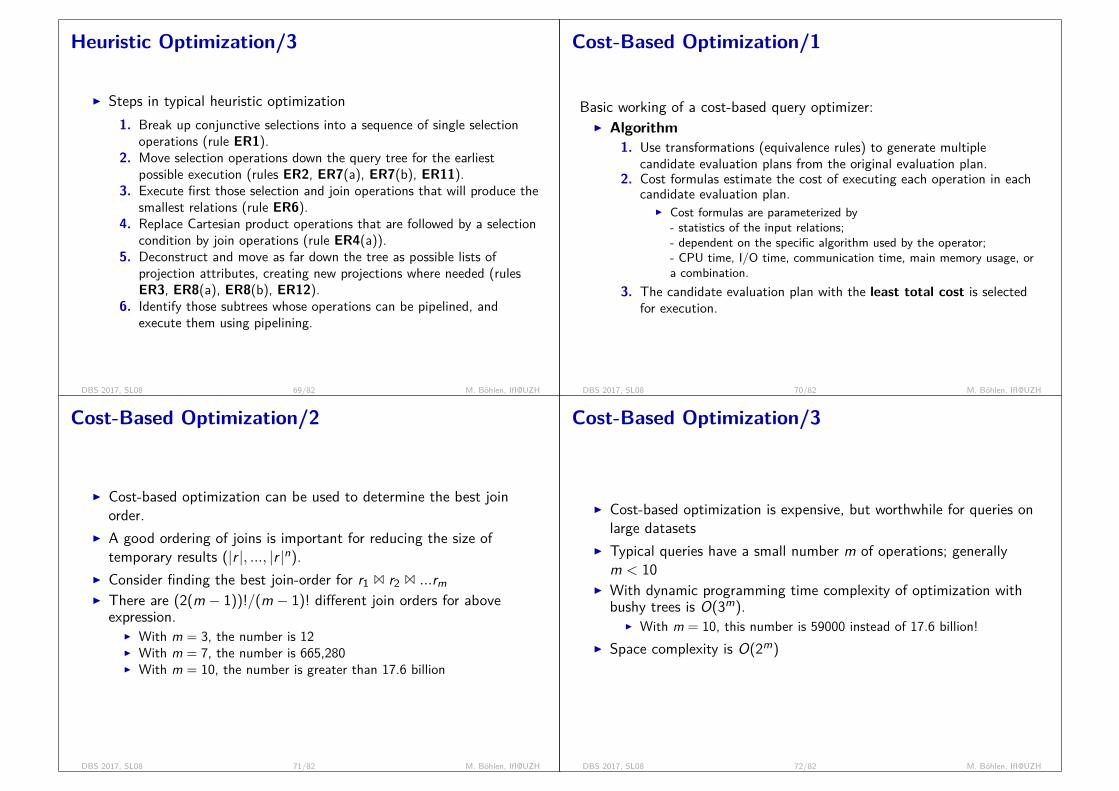
Heuristic Optimization/3
I Steps in typical heuristic optimization1. Break up conjunctive selections into a sequence of single selection
operations (rule ER1).2. Move selection operations down the query tree for the earliest
possible execution (rules ER2, ER7(a), ER7(b), ER11).3. Execute first those selection and join operations that will produce the
smallest relations (rule ER6).4. Replace Cartesian product operations that are followed by a selection
condition by join operations (rule ER4(a)).5. Deconstruct and move as far down the tree as possible lists of
projection attributes, creating new projections where needed (rulesER3, ER8(a), ER8(b), ER12).
6. Identify those subtrees whose operations can be pipelined, andexecute them using pipelining.
DBS 2017, SL08 69/82 M. Böhlen, IfI@UZH
Cost-Based Optimization/1
Basic working of a cost-based query optimizer:I Algorithm
1. Use transformations (equivalence rules) to generate multiplecandidate evaluation plans from the original evaluation plan.
2. Cost formulas estimate the cost of executing each operation in eachcandidate evaluation plan.
I Cost formulas are parameterized by- statistics of the input relations;- dependent on the specific algorithm used by the operator;- CPU time, I/O time, communication time, main memory usage, ora combination.
3. The candidate evaluation plan with the least total cost is selectedfor execution.
DBS 2017, SL08 70/82 M. Böhlen, IfI@UZH
Cost-Based Optimization/2
I Cost-based optimization can be used to determine the best joinorder.
I A good ordering of joins is important for reducing the size oftemporary results (|r |, ..., |r |n).
I Consider finding the best join-order for r1 1 r2 1 ...rmI There are (2(m − 1))!/(m − 1)! different join orders for above
expression.I With m = 3, the number is 12I With m = 7, the number is 665,280I With m = 10, the number is greater than 17.6 billion
DBS 2017, SL08 71/82 M. Böhlen, IfI@UZH
Cost-Based Optimization/3
I Cost-based optimization is expensive, but worthwhile for queries onlarge datasets
I Typical queries have a small number m of operations; generallym < 10
I With dynamic programming time complexity of optimization withbushy trees is O(3m).
I With m = 10, this number is 59000 instead of 17.6 billion!I Space complexity is O(2m)
DBS 2017, SL08 72/82 M. Böhlen, IfI@UZH

Review 8.8Consider a DB with the following characteristics:
I |r1(A,B,C)| = 1000,V (C , r1) = 900I |r2(C ,D,E )| = 1500,V (C , r2) = 1100,V (E , r2) = 50I |r3(E ,F )| = 750,V (E , r3) = 100
Estimate the size of r1 1 r2 1 r3 and determine an efficient evaluationstrategy.
DBS 2017, SL08 73/82 M. Böhlen, IfI@UZH
Cost-Based Optimization Example/1
I Example: σSSN=0810643773(Emp)I Statistics:
I |Emp| = 10’000 tuplesI 5 tuples per blockI Secondary B+-tree index of depth 4 on SSNI SSN is primary key
I Plan p1: full table scanI cost(p1) = (10’000/5)/2 = 1’000 blocks
I Plan p2: B+-tree lookupI cost(p2) = 4 + 1 = 5 blocks
DBS 2017, SL08 74/82 M. Böhlen, IfI@UZH
Cost-Based Optimization Example/2
I Example: σDNo>15(Emp)I Statistics:
I |Emp| = 10’000 tuplesI 5 tuples per blockI Primary index on DNo of depth 2I 50 different departments
I Plan p1: full table scanI cost (p1) = 10’000/5 = 2’000 blocks
I Plan p2: index searchI cost(p2) = 2 + (50-15)/50*(10’000/5) = 1’400 blocks
DBS 2017, SL08 75/82 M. Böhlen, IfI@UZH
Cost-Based Optimization Example/3
I Emp 1DNo=DNum DeptI Statistics:
I |Emp| = 10’000 tuples ; 5 Emp tuples per blockI |Dept| = 125; 10 Dept tuples per blockI Hash index on Emp(DNo)I 4 EmpDept result tuples per block
I Plan p1: Block nested loop with Emp as outer loopI cost(p1) = (10’000/5) + (10’000/5) * (125/10) + (10’000/4)
= 30’500 IOsI (10.000/4 is cost of writing final output)
I Plan p2: Indexed nested loop with Dept as outer loop and hashedlookup in Emp
I cost(p2) = (125/10) + 125 * (10’000/125/5) + (10’000/4)= 4’513 IOs
I 10’000/125/5 is the average number of blocks/department
DBS 2017, SL08 76/82 M. Böhlen, IfI@UZH

PostgreSQL Query Optimization/1
DBS 2017, SL08 77/82 M. Böhlen, IfI@UZH
PostgreSQL Query Optimization/2
DBS 2017, SL08 78/82 M. Böhlen, IfI@UZH
PostgreSQL Query Optimization/3
DBS 2017, SL08 79/82 M. Böhlen, IfI@UZH
PostgreSQL Query Optimization/4
DBS 2017, SL08 80/82 M. Böhlen, IfI@UZH
Summary/1
I Query evaluation techniques:
I Physical sorting:I Physical sorting is a basic and important techniqueI The same sort order should be useful to many operators and not just
one (global optimization versus local optimization)
I Evaluation techniques for selections:I Use primary index if available; secondary index is much worseI Equality conditions are selective and should be optimizedI Linear scan with sequential IO is the base line for selections
I Evaluation techniques for joins:I nested loop: base line; avoid whenever possibleI sort merge: robust and fastI hash join: fastest; only for equality
DBS 2017, SL08 81/82 M. Böhlen, IfI@UZH
Summary/2
I Query optimization techniques
I Equivalence rules for relational algebra expressions (must hold formultisets)
I Rule-based query optimization is based on heuristics (usually thegoal is to keep intermediate results as small as possible)
I Cost-based query optimization uses statistical information to findthe cheapest (or reasonably cheap) plan
DBS 2017, SL08 82/82 M. Böhlen, IfI@UZH
Database SystemsSpring 2017
Transaction ProcessingSL09
I Transactions
ex: booking a trip (reserve flight, hotel, car: sequence?)
I ACID Properties, Schedules, Serializability, RecoverabilityI Concurrency Control
Mehrbenutzerbetrieb
I Lock-based Protocols, Transactions in SQL, Deadlock HandlingI Recovery System
error handling, Wiederherstellung
I Log-Based Recovery, Deferred/Immediate Modifications
Reviews: 23 41 42 45 46 50 51 52 74
DBS 2017, SL09 1/78 M. Böhlen, IfI@UZH
Literature and Acknowledgments
Reading List for SL09:I Database Systems, Chapters 20, 21, and 22, Sixth Edition, Ramez
Elmasri and Shamkant B. Navathe, Pearson Education, 2010.
These slides were developed by:I Michael Böhlen, University of Zürich, SwitzerlandI Johann Gamper, Free University of Bozen-Bolzano, Italy
The slides are based on the following text books and associated material:I Database Systems, Sixth Edition, Ramez Elmasri and Shamkant B.
Navathe, Pearson Addison Wesley, 2004.I A. Silberschatz, H. Korth, and S. Sudarshan: Database System
Concepts, McGraw Hill, 2006.
DBS 2017, SL09 2/78 M. Böhlen, IfI@UZH
Transaction Concept
I Transaction: A logical unit of program execution (i.e., a sequenceof actions) that accesses and possibly updates various data items. Atransaction is never executed partially and it includes one or moreDB access operations (insertion, deletion, modification, retrieval)
I For a transaction the following must hold:I A transaction must see a consistent databaseI During transaction execution the DB may be inconsistent.I When the transaction is committed, the DB must be consistent
I Two main issues to deal with:I Concurrent execution of multiple transactionsI Various failures, e.g., hardware failures and system crashes
Finalizing a transaction is necessary. DBMS will finali-ze transaction when connection/session is closed; it cancommit or rollback all changes. 100k tuples inserted, lo-gout: what happens?!
DBS 2017, SL09 3/78 M. Böhlen, IfI@UZH
Transactions
I Transaction StatesI ACID PropertiesI SchedulesI SerializabilityI Recoverability
DBS 2017, SL09 4/78 M. Böhlen, IfI@UZH
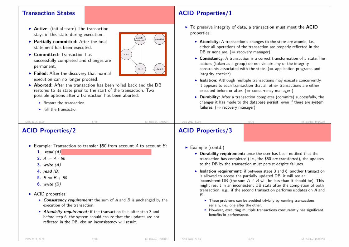
Transaction States
Finalising a transaction is necessary (either commit orabort); example: insert 100K tuple, quit pgadmin, db andapplication may decide to keep or throw away the insertedtuples
I Active: (initial state) The transactionstays in this state during execution.
I Partially committed: After the finalstatement has been executed.
I Committed: Transaction hassuccessfully completed and changes arepermanent.
I Failed: After the discovery that normalexecution can no longer proceed.
I Aborted: After the transaction has been rolled back and the DBrestored to its state prior to the start of the transaction. Twopossible options after a transaction has been aborted:
I Restart the transactionI Kill the transaction
DBS 2017, SL09 5/78 M. Böhlen, IfI@UZH
ACID Properties/1
I To preserve integrity of data, a transaction must meet the ACIDproperties:
I Atomicity: A transaction’s changes to the state are atomic, i.e.,either all operations of the transaction are properly reflected in theDB or none are. (⇒ recovery manager)
I Consistency: A transaction is a correct transformation of a state.Theactions (taken as a group) do not violate any of the integrityconstraints associated with the state. (⇒ application programs andintegrity checker)
I Isolation: Although multiple transactions may execute concurrently,it appears to each transaction that all other transactions are eitherexecuted before or after. (⇒ concurrency manager )
I Durability: After a transaction completes (commits) successfully, thechanges it has made to the database persist, even if there are systemfailures. (⇒ recovery manager)
DBS 2017, SL09 6/78 M. Böhlen, IfI@UZH
ACID Properties/2
I Example: Transaction to transfer $50 from account A to account B:1. read (A)
A is unit in DB; tuple or attr or table; mostly attr for us
2. A := A - 503. write (A)4. read (B)5. B := B + 506. write (B)
I ACID properties:I Consistency requirement: the sum of A and B is unchanged by the
execution of the transaction.I Atomicity requirement: if the transaction fails after step 3 and
before step 6, the system should ensure that the updates are notreflected in the DB, else an inconsistency will result.
DBS 2017, SL09 7/78 M. Böhlen, IfI@UZH
ACID Properties/3
I Example (contd.)I Durability requirement: once the user has been notified that the
transaction has completed (i.e., the $50 are transferred), the updatesto the DB by the transaction must persist despite failures.
I Isolation requirement: if between steps 3 and 6, another transactionis allowed to access the partially updated DB, it will see aninconsistent DB (the sum A + B will be less than it should be). Thismight result in an inconsistent DB state after the completion of bothtransaction, e.g., if the second transaction performs updates on A andB.
I These problems can be avoided trivially by running transactionsserially, i.e., one after the other.
I However, executing multiple transactions concurrently has significantbenefits in performance.
we want either < T1; T2 > (T1 followed by T2) or< T2; T1 > (T2 followed by T1). which one is irrele-vant. there is no absolute time (changing order is OK;no fairness; similar to printing or teller machine)
DBS 2017, SL09 8/78 M. Böhlen, IfI@UZH

ACID Properties/4
I The recovery manager of a DBMS implements the support foratomicity and durability.
I The concurrency control system restricts the interactions betweenconcurrent transactions in order to ensure isolation.
I Advantages of running multiple transactions concurrently in thesystem:
I increased processor and disk utilization, leading to bettertransaction throughput: one transaction can use the CPU whileanother reads from or writes to the disk
I reduced average response time for transactions: short transactionsneed not wait behind long ones.
I It is the task of application programs to ensure consistency:I Each transaction preserves DB consistency.I Serial execution of a set of transactions preserves DB consistency.
DBS 2017, SL09 9/78 M. Böhlen, IfI@UZH
Schedules/1
I Schedule (or history): Sequence of instructions from a set ofconcurrent transactions that indicate the chronological order inwhich these instructions are executed.
I Must consist of all instructions of all transactions.I Must preserve the order of instructions within each individual
transaction.I Serial schedule: Transactions execute one after the other.
I One transaction is completely finished before another transactionstarts.
DBS 2017, SL09 10/78 M. Böhlen, IfI@UZH
Schedules/2
I Example: Consider the following transactions:I T1 transfers $50 from A to B
A: 200 to 150, B: 300 to 350
I T2 transfers 10% of the balance from A to B
A: 150 to 135, B: 350 to 365
I The following is a serial schedule, i.e.,< T1;T2 >, in which T1 is followed by T2.
I Integrity constraintI Sum of A + B is preserved
DBS 2017, SL09 11/78 M. Böhlen, IfI@UZH
Schedules/3
200 to 150
300 to 350
150 to 135
350 to 365
I Example: (contd.)I The following schedule is not a serial schedule, but it is equivalent
to the previous one (i.e., gives the same result).I In both schedules the sum of A + B is preserved.
DBS 2017, SL09 12/78 M. Böhlen, IfI@UZH
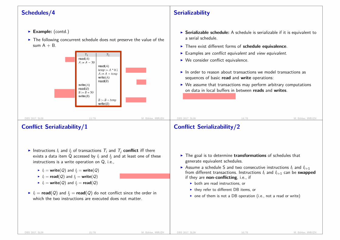
Schedules/4
200
200 to 150300 to 350
200 to 180
300
300 to 320
I Example: (contd.)I The following concurrent schedule does not preserve the value of the
sum A + B.
DBS 2017, SL09 13/78 M. Böhlen, IfI@UZH
Serializability
I Serializable schedule: A schedule is serializable if it is equivalent toa serial schedule.
I There exist different forms of schedule equivalence.I Examples are conflict equivalent and view equivalent.I We consider conflict equivalence.
I In order to reason about transactions we model transactions assequences of basic read and write operations:
I We assume that transactions may perform arbitrary computationson data in local buffers in between reads and writes.
read(X); X can change; write(X)
DBS 2017, SL09 14/78 M. Böhlen, IfI@UZH
Conflict Serializability/1
I Instructions li and lj of transactions Ti and Tj conflict iff thereexists a data item Q accessed by li and lj and at least one of theseinstructions is a write operation on Q, i.e.,
I li = write(Q) and lj = write(Q)I li = read(Q) and lj = write(Q)I li = write(Q) and lj = read(Q)
I li = read(Q) and lj = read(Q) do not conflict since the order inwhich the two instructions are executed does not matter.
old and new value are different
DBS 2017, SL09 15/78 M. Böhlen, IfI@UZH
Conflict Serializability/2
I The goal is to determine transformations of schedules thatgenerate equivalent schedules.
I Assume a schedule S and two consecutive instructions Ii and Ii+1from different transactions. Instructions Ii and Ii+1 can be swappedif they are non-conflicting, i.e., if
I both are read instructions, orI they refer to different DB items, orI one of them is not a DB operation (i.e., not a read or write)
DBS 2017, SL09 16/78 M. Böhlen, IfI@UZH
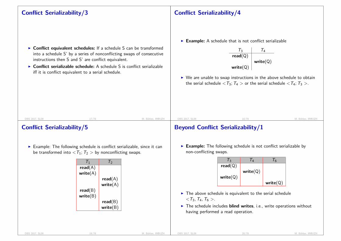
Conflict Serializability/3
I Conflict equivalent schedules: If a schedule S can be transformedinto a schedule S’ by a series of nonconflicting swaps of consecutiveinstructions then S and S’ are conflict equivalent.
I Conflict serializable schedule: A schedule S is conflict serializableiff it is conflict equivalent to a serial schedule.
DBS 2017, SL09 17/78 M. Böhlen, IfI@UZH
Conflict Serializability/4
I Example: A schedule that is not conflict serializable
T3 T4read(Q)
write(Q)write(Q)
I We are unable to swap instructions in the above schedule to obtainthe serial schedule <T3;T4 > or the serial schedule <T4;T3 >.
DBS 2017, SL09 18/78 M. Böhlen, IfI@UZH
Conflict Serializability/5
I Example: The following schedule is conflict serializable, since it canbe transformed into <T1;T2 > by nonconflicting swaps.
T1 T2read(A)write(A)
read(A)write(A)
read(B)write(B)
read(B)write(B)
DBS 2017, SL09 19/78 M. Böhlen, IfI@UZH
Beyond Conflict Serializability/1
I Example: The following schedule is not conflict serializable bynon-conflicting swaps.
T3 T4 T6read(Q)
write(Q)write(Q)
write(Q)
I The above schedule is equivalent to the serial schedule<T3,T4,T6 >.
I The schedule includes blind writes, i.e., write operations withouthaving performed a read operation.
DBS 2017, SL09 20/78 M. Böhlen, IfI@UZH
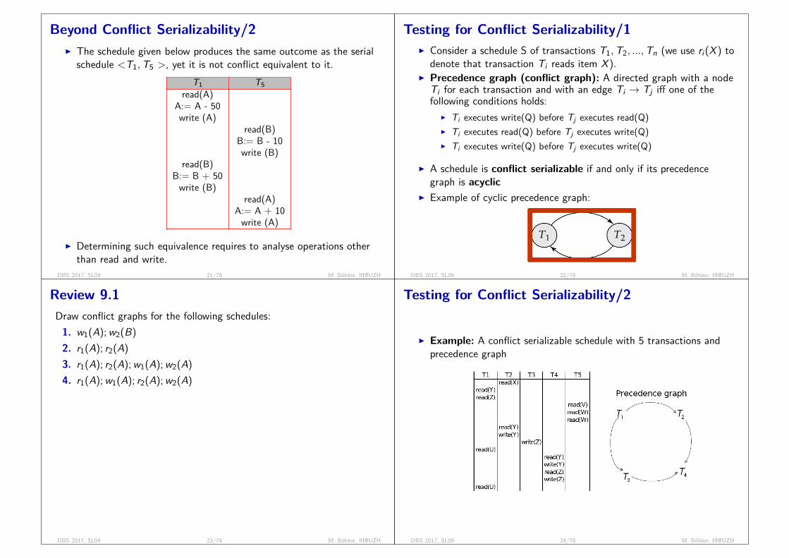
Beyond Conflict Serializability/2I The schedule given below produces the same outcome as the serial
schedule <T1,T5 >, yet it is not conflict equivalent to it.T1 T5
read(A)A:= A - 50write (A)
read(B)B:= B - 10write (B)
read(B)B:= B + 50write (B)
read(A)A:= A + 10write (A)
I Determining such equivalence requires to analyse operations otherthan read and write.
DBS 2017, SL09 21/78 M. Böhlen, IfI@UZH
Testing for Conflict Serializability/1I Consider a schedule S of transactions T1,T2, ...,Tn (we use ri(X ) to
denote that transaction Ti reads item X ).I Precedence graph (conflict graph): A directed graph with a node
Ti for each transaction and with an edge Ti → Tj iff one of thefollowing conditions holds:
I Ti executes write(Q) before Tj executes read(Q)I Ti executes read(Q) before Tj executes write(Q)I Ti executes write(Q) before Tj executes write(Q)
I A schedule is conflict serializable if and only if its precedencegraph is acyclic
I Example of cyclic precedence graph:
DBS 2017, SL09 22/78 M. Böhlen, IfI@UZH
Review 9.1Draw conflict graphs for the following schedules:1. w1(A);w2(B)2. r1(A); r2(A)3. r1(A); r2(A);w1(A);w2(A)4. r1(A);w1(A); r2(A);w2(A)
1. T1 T2T1 T2
2. T1 T2T1 T2
3. T1 < − > T2T1 T2
4. T1 − > T2T1 T2
DBS 2017, SL09 23/78 M. Böhlen, IfI@UZH
Testing for Conflict Serializability/2
I Example: A conflict serializable schedule with 5 transactions andprecedence graph
DBS 2017, SL09 24/78 M. Böhlen, IfI@UZH
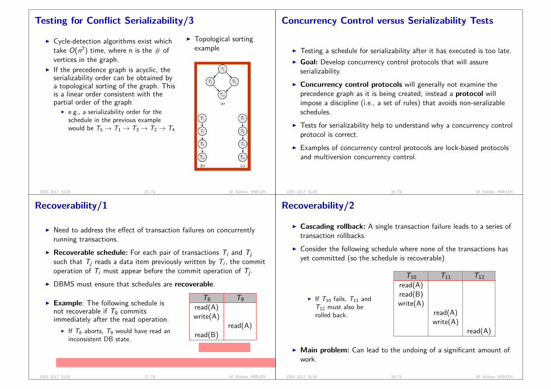
Testing for Conflict Serializability/3
I Cycle-detection algorithms exist whichtake O(n2) time, where n is the # ofvertices in the graph.
I If the precedence graph is acyclic, theserializability order can be obtained bya topological sorting of the graph. Thisis a linear order consistent with thepartial order of the graph
I e.g., a serializability order for theschedule in the previous examplewould be T5 → T1 → T3 → T2 → T4
I Topological sortingexample
DBS 2017, SL09 25/78 M. Böhlen, IfI@UZH
Concurrency Control versus Serializability Tests
I Testing a schedule for serializability after it has executed is too late.I Goal: Develop concurrency control protocols that will assure
serializability.I Concurrency control protocols will generally not examine the
precedence graph as it is being created; instead a protocol willimpose a discipline (i.e., a set of rules) that avoids non-seralizableschedules.
I Tests for serializability help to understand why a concurrency controlprotocol is correct.
I Examples of concurrency control protocols are lock-based protocolsand multiversion concurrency control.
DBS 2017, SL09 26/78 M. Böhlen, IfI@UZH
Recoverability/1
I Need to address the effect of transaction failures on concurrentlyrunning transactions.
I Recoverable schedule: For each pair of transactions Ti and Tjsuch that Tj reads a data item previously written by Ti , the commitoperation of Ti must appear before the commit operation of Tj .
I DBMS must ensure that schedules are recoverable.
I Example: The following schedule isnot recoverable if T9 commitsimmediately after the read operation.
I If T8 aborts, T9 would have read aninconsistent DB state.
T8 T9read(A)write(A)
read(A)read(B)
T9 depends on T8
T9 must commit after T8; T8 commit => T9 commit or abort; T8 abort => T9 abort
DBS 2017, SL09 27/78 M. Böhlen, IfI@UZH
Recoverability/2
I Cascading rollback: A single transaction failure leads to a series oftransaction rollbacks.
I Consider the following schedule where none of the transactions hasyet committed (so the schedule is recoverable)
I If T10 fails, T11 andT12 must also berolled back.
T10 T11 T12read(A)read(B)write(A)
read(A)write(A)
read(A)
I Main problem: Can lead to the undoing of a significant amount ofwork.
DBS 2017, SL09 28/78 M. Böhlen, IfI@UZH
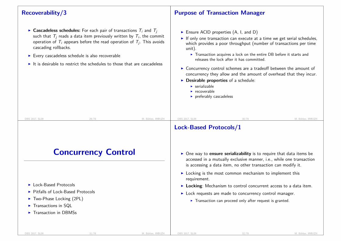
Recoverability/3
I Cascadeless schedules: For each pair of transactions Ti and Tjsuch that Tj reads a data item previously written by Ti , the commitoperation of Ti appears before the read operation of Tj . This avoidscascading rollbacks.
I Every cascadeless schedule is also recoverableI It is desirable to restrict the schedules to those that are cascadeless
DBS 2017, SL09 29/78 M. Böhlen, IfI@UZH
Purpose of Transaction Manager
I Ensure ACID properties (A, I, and D)I If only one transaction can execute at a time we get serial schedules,
which provides a poor throughput (number of transactions per timeunit).
I Transaction acquires a lock on the entire DB before it starts andreleases the lock after it has committed.
I Concurrency control schemes are a tradeoff between the amount ofconcurrency they allow and the amount of overhead that they incur.
I Desirable properties of a schedule:I serializableI recoverableI preferably cascadeless
DBS 2017, SL09 30/78 M. Böhlen, IfI@UZH
Concurrency Control
I Lock-Based ProtocolsI Pitfalls of Lock-Based ProtocolsI Two-Phase Locking (2PL)I Transactions in SQLI Transaction in DBMSs
DBS 2017, SL09 31/78 M. Böhlen, IfI@UZH
Lock-Based Protocols/1
I One way to ensure serializability is to require that data items beaccessed in a mutually exclusive manner, i.e., while one transactionis accessing a data item, no other transaction can modify it.
I Locking is the most common mechanism to implement thisrequirement.
I Locking: Mechanism to control concurrent access to a data item.I Lock requests are made to concurrency control manager.
I Transaction can proceed only after request is granted.
DBS 2017, SL09 32/78 M. Böhlen, IfI@UZH

Lock-Based Protocols/2
I Data items can be locked in two modes:I exclusive mode (X): Data item can be both read as well as written.
X-lock is requested using X-lock(A) instruction.I shared mode (S): Data item can only be read. S-lock is requested
using S-lock(A) instruction.
I Locks can be released: U-lock(A)I Locking protocol: A set of rules followed by all transactions while
requesting and releasing locks.I Locking protocols restrict the set of possible schedules.
I Ensure serializable schedules by delaying transactions that mightviolate serializability.
DBS 2017, SL09 33/78 M. Böhlen, IfI@UZH
Lock-Based Protocols/3I Lock-compatibility matrix tells whether two locks are compatible
or not.I Any number of transactions
can hold shared locks on adata item
I If any transaction holds anexclusive lock on a data itemno other transaction mayhold any lock on that item.
lock 1
lock 2S X
S TRUE FALSEX FALSE FALSE
I Locking Rules/ProtocolI A transaction may be granted a lock on an item if the requested lock
is compatible with locks already held on the item by othertransactions.
I If a lock cannot be granted, the requesting transaction is made towait until all incompatible locks held by other transactions have beenreleased. The lock is then granted.
DBS 2017, SL09 34/78 M. Böhlen, IfI@UZH
Pitfalls of Lock-Based Protocols/1
I Too early unlocking can lead to non-serializable schedules.I Too late unlocking can lead to deadlocks.
I ExampleI Transaction T1 transfers $50 from account B to account A.I Transaction T2 displays the total amount of money in accounts A
and B, that is, the sum A + B.
DBS 2017, SL09 35/78 M. Böhlen, IfI@UZH
Pitfalls of Lock-Based Protocols/2I Example (contd.): Early unlocking can cause non-serializableschedules, and therefore potentially incorrect results.
I e.g., A = $100, B = $200I displaying A + B shows $250I < T1;T2 > and < T2;T1 >
display $300
T1 T21. X-lock(B)2. read B3. B := B-504. write B5. U-lock(B)6. S-lock(A)7. read A8. U-lock(A)9. S-lock(B)10. read B11. U-lock(B)12. display A + B13. X-lock(A)14. read A15. A := A+5016. write A17. U-lock(A)
DBS 2017, SL09 36/78 M. Böhlen, IfI@UZH

Pitfalls of Lock-Based Protocols/3
I Example (contd.): Late unlocking can lead to deadlocks(transactions block each other)
T1 T21. X-lock(B)2. read B3. B := B-504. write B5. S-lock(A)6. read A7. S-lock(B)8. X-lock(A)
has got B, waits for Ahas got A, waits for B
I Neither T1 nor T2 can make progress:I S-lock(B) causes T2 to wait for T1 to release its lock on B.I X-lock(A) causes T1 to wait for T2 to release its lock on A
I To handle a deadlock one of T1 or T2 must be rolled back and itslocks released.
DBS 2017, SL09 37/78 M. Böhlen, IfI@UZH
Two-Phase Locking Protocol/1
I Two-Phase Locking Protocol: A locking protocol that ensuresconflict-serializable schedules. It works in two phases:
I Phase 1: Growing PhaseI transaction may obtain locksI transaction may not release locks
I Phase 2: Shrinking PhaseI transaction may release locksI transaction may not obtain locks
I Lock point: Transition point form phase 1 into phase 2, i.e., whenthe first lock is released.
DBS 2017, SL09 38/78 M. Böhlen, IfI@UZH
Two-Phase Locking Protocol/2I Example: Schedule with locking instructions following the
Two-Phase Locking ProtocolT1 T2
1. X-lock(B)2. read B3. B := B-504. write B5. X-lock(A)6. U-lock(B)7. S-lock(B)8. read(B)9. read(A)10. A := A+5011. write(A)12. U-lock(A)13. S-lock(A)14. read(A)15. display A + B16. U-lock(B)17. U-lock(A)
T1: grows from 1. to 5.;shrinks from 6. to 17.
T2 grows from 7. to 15.;shrinks from 16. to 17.
DBS 2017, SL09 39/78 M. Böhlen, IfI@UZH
Two-Phase Locking Protocol/3I Properties of the Two-Phase Locking Protocol
I Ensures serializabilityI It can be shown that the transactions can be serialized in the order of
their lock points (i.e., the point when a transaction acquired its finallock).
I Does not ensure freedom from deadlocksI Cascading rollback is possible
I Modifications of the two-phase locking protocolI Strict two-phase locking (S2PL)
I A transaction must hold all its exclusive locks until itcommits/aborts
I Avoids cascading rollbackI Rigorous two-phase locking (SS2PL)
simple to implement; noknowledge about tran-saction required
I All locks are held till commit/abort.I Transactions can be serialized in the order in which they commit.
DBS 2017, SL09 40/78 M. Böhlen, IfI@UZH

Review 9.2Use Venn diagrams to relate1. serial schedules (SS)2. schedules (S)3. conflict serializable schedules (CSS)4. correct schedules (CS)5. two-phase locking schedules (2PL)
and give representative examples.
SS
2PL
CSS
CS
DBS 2017, SL09 41/78 M. Böhlen, IfI@UZH
Review 9.3Consider transactionsT1: r(A); r(B); if A=0 then B:=B+1; w(B)T2: r(B); r(A); if B=0 then A:=A+1; w(A)Add lock and unlock instructions that follow 2PL. Show a 2PL schedulethat leads to a deadlock?
T1 T2S-l(A) S-l(B)r(A) r(B)X-l(B) X-l(A)r(B) r(A)if A = ... if B = ...w(B) w(A)U-l(A) U-l(B)U-l(B) U-l(A)
T1 T2S-l(A)
S-l(B)r(B)
r(A)X-l(B)
X-l(B)DEADLOCK
DBS 2017, SL09 42/78 M. Böhlen, IfI@UZH
Transactions in SQL/1
I The SQL standard defines three undesired phenomena oftransactions:
I dirty read: a transaction sees changes from other uncommittedtransactions
I nonrepeatable read: if a transactions retrieves a row twice it getsdifferent answers
I phantom reads: if a transaction retrieves a range of rows twice itretrieves a different answer
DBS 2017, SL09 43/78 M. Böhlen, IfI@UZH
Transactions in SQL/2
I The SQL standard uses the undesired phenomena to define fourisolation levels as follows:
PhenomenaIsolation level
Dirty read Nonrepeatableread
Phantomread
read uncommitted yes yes yesread committed no yes yesrepeatable read no no yesserializable no no no
DBS 2017, SL09 44/78 M. Böhlen, IfI@UZH

Review 9.4/1
Assume r(a) = {(1), (2), (3)} and isolation levels read committed, readuncommitted, and serializability. What is the behavior of schedule:
T1: UPDATE p SET a=5 WHERE a=1
T2: SELECT * FROM p;
RC: {(1),(2),(3)}, RU: {(5),(2),(3)}, SER: block
T1: COMMIT;
RC: done, RU: done, SER: done and T2 unblocked{(5),(2),(3)}
T2: SELECT * FROM p;
RC: {(5),(2),(3)}, RU: {(5),(2),(3)}, SER: {(5),(2),(3)}
DBS 2017, SL09 45/78 M. Böhlen, IfI@UZH
Review 9.4/2Assume relation r(a) = {(1), (2), (3)} and isolation level read committed.What is the behavior of the following schedule:T1: UPDATE p SET a=5 WHERE a=1;T2: UPDATE p SET a=5 WHERE a=1;T1: COMMIT;
1 tuple updated (T1)
blocked (T2)
committed(T1)no row found for update (T2)
DBS 2017, SL09 46/78 M. Böhlen, IfI@UZH
Transactions in DBMSs/1
I Database systems do not always make serializable the defaultisolation level.
I The SQL commands COMMIT and ROLLBACK finish the runningtransaction.
I Some database systems issue autocommits after each statement orat the end of sessions.
I PostgreSQL has a command BEGIN to start a transaction.I Applications programs (graphical tools, etc) might implement their
own transaction handling by issuing COMMIT and ROLLBACK.I SQL does not permit to mix DDL and DML statement inside a
transaction.
DBS 2017, SL09 47/78 M. Böhlen, IfI@UZH
Transactions in DBMSs/2
I In order to increase performance (throughput) more and moreDBMSs offer MVCC (multiversion concurrency control) rather than2PL.
I Systems that use MVCC (Oracle, PostgreSQL) and 2PL (DB2,MySQL) behave differently.
I With MVCC the isolation level serializable does not permit dirtyreads, nonrepeatable reads, and phantom reads (as required by theSQL standard), but true serializability is not guaranteed.
I With MVCC explicit locks must be used by the application to getserializability: SELECT * FROM p FOR UPDATE;
DBS 2017, SL09 48/78 M. Böhlen, IfI@UZH
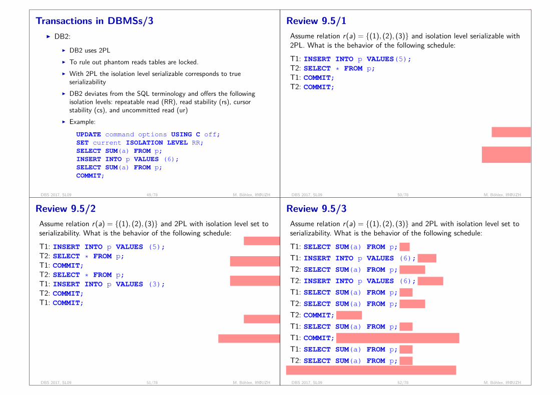
Transactions in DBMSs/3I DB2:
I DB2 uses 2PLI To rule out phantom reads tables are locked.I With 2PL the isolation level serializable corresponds to true
serializabilityI DB2 deviates from the SQL terminology and offers the following
isolation levels: repeatable read (RR), read stability (rs), cursorstability (cs), and uncommitted read (ur)
I Example:UPDATE command options USING C off;SET current ISOLATION LEVEL RR;SELECT SUM(a) FROM p;INSERT INTO p VALUES (6);SELECT SUM(a) FROM p;COMMIT;
DBS 2017, SL09 49/78 M. Böhlen, IfI@UZH
Review 9.5/1Assume relation r(a) = {(1), (2), (3)} and isolation level serializable with2PL. What is the behavior of the following schedule:T1: INSERT INTO p VALUES(5);T2: SELECT * FROM p;T1: COMMIT;T2: COMMIT;
blocked (T2)
committed(T1){1, 2, 3, 5} (T2)
DBS 2017, SL09 50/78 M. Böhlen, IfI@UZH
Review 9.5/2Assume relation r(a) = {(1), (2), (3)} and 2PL with isolation level set toserializability. What is the behavior of the following schedule:T1: INSERT INTO p VALUES (5);T2: SELECT * FROM p;T1: COMMIT;T2: SELECT * FROM p;T1: INSERT INTO p VALUES (3);T2: COMMIT;T1: COMMIT;
T2: blocked
T2: { 2, 3, 6, 1 }
T2: { 2, 3, 6, 1 }
T1: blocked
T1: insertion executed
DBS 2017, SL09 51/78 M. Böhlen, IfI@UZH
Review 9.5/3Assume relation r(a) = {(1), (2), (3)} and 2PL with isolation level set toserializability. What is the behavior of the following schedule:T1: SELECT SUM(a) FROM p;
6
T1: INSERT INTO p VALUES (6);
done
T2: SELECT SUM(a) FROM p;
blocked
T2: INSERT INTO p VALUES (6);
blocked
T1: SELECT SUM(a) FROM p;
12
T2: SELECT SUM(a) FROM p;
blocked
T2: COMMIT;
blocked
T1: SELECT SUM(a) FROM p;
12
T1: COMMIT;
done; T2: 12; done (insert); 18; done (commit)
T1: SELECT SUM(a) FROM p;
18
T2: SELECT SUM(a) FROM p;
18transaction order: < T1, T2; T1’; T2’ > or < T1, T2; T2’; T1’ >
DBS 2017, SL09 52/78 M. Böhlen, IfI@UZH

Deadlock Handling/1
I Consider the following two transactions:T1: write (A) T2: write(B)
write(B) write(A)I Schedule with deadlock
T1 T2X-lock(A)write(A)
X-lock(B)write(B)waits for X-lock on A
waits for X-lock on B
DBS 2017, SL09 53/78 M. Böhlen, IfI@UZH
Deadlock Handling/2
I Deadlock: A system is in a deadlock state if there is a set oftransactions such that every transaction in the set is waiting foranother transaction in the set.
I A deadlock has to be resolved by rolling back some of thetransactions involved in the deadlock.
I Deadlocks are addressed in two ways:I Deadlock prevention protocols are usedI Deadlocks are detected and resolved
DBS 2017, SL09 54/78 M. Böhlen, IfI@UZH
Deadlock Prevention Protocols
I Deadlock prevention protocols ensure that the system will neverenter into a deadlock state.
I Two deadlock prevention protocols are wait-die and wound-wait.They use transaction timestamps to prevent deadlocks.
I With both protocols rolled-back transactions are restarted with theiroriginal timestamp. Since older transactions have precedence overnewer ones starvation is avoided.
I Timeout-based protocols can be used to avoid deadlocks:I A transaction waits for a lock only for a specified amount of time.
After that, the wait times out and the transaction is rolled back.I Thus deadlocks are not possible.I Simple to implement; but starvation is possible. Also difficult to
determine good value of the timeout interval.
DBS 2017, SL09 55/78 M. Böhlen, IfI@UZH
Deadlock Detection and Recovery/1
I Deadlocks can be described as a wait-for graph, which consists of apair G = (V,E),
I V is a set of vertices representing all the transactionsI E is a set of edges; each element is an ordered pair Ti → Tj .
I If Ti → Tj is in E, there is a directed edge from Ti to Tj , implyingthat Ti is waiting for Tj to release a data item.
I If Ti requests a data item being held by Tj , edge Ti → Tj isinserted in the wait-for graph. This edge is removed when Tj is nolonger holding a data item needed by Ti .
I The system is in a deadlock state if and only if the wait-for graphhas a cycle. Must invoke a deadlock-detection algorithm periodicallyto look for cycles.
DBS 2017, SL09 56/78 M. Böhlen, IfI@UZH

Deadlock Detection and Recovery/2
I Wait-for graph without a cycleI Wait-for graph with a
cycle
DBS 2017, SL09 57/78 M. Böhlen, IfI@UZH
Deadlock Detection and Recovery/3
I When a deadlock is detected, the system must recover from thedeadlock.
I The most common solution is to roll back one or more transactionsto break the deadlock. Three actions are required:1. Selection of a victim: For rollback select the transaction(s) that will
incur minimum cost.2. Rollback: Determine how far to roll back transaction
I Total rollback: Abort the transaction and then restart it.I Partial rollback: roll back transaction only as far as necessary to break
deadlock.3. Check Starvation: happens if same transaction is always chosen as
victim.I Include the number of rollbacks in the cost factor to avoid starvation
DBS 2017, SL09 58/78 M. Böhlen, IfI@UZH
Recovery System
I Log-Based RecoveryI Deferred DB ModificationsI Immediate DB ModificationsI Checkpoints
DBS 2017, SL09 59/78 M. Böhlen, IfI@UZH
Recovery System/1
I Recovery system: Ensures atomicity and durability of transactionsin the presence of failures (and concurrent transactions).
I Atomicity and durability properties of transactions:I A transaction either completes fully with a permanent result (i.e.,
committed transaction)I or does not happen at all and has no effect on the DB (i.e.,
aborted/rolled-back transaction if some error occurs)I Transactions are aborted or rolled-back if some error occurs
DBS 2017, SL09 60/78 M. Böhlen, IfI@UZH
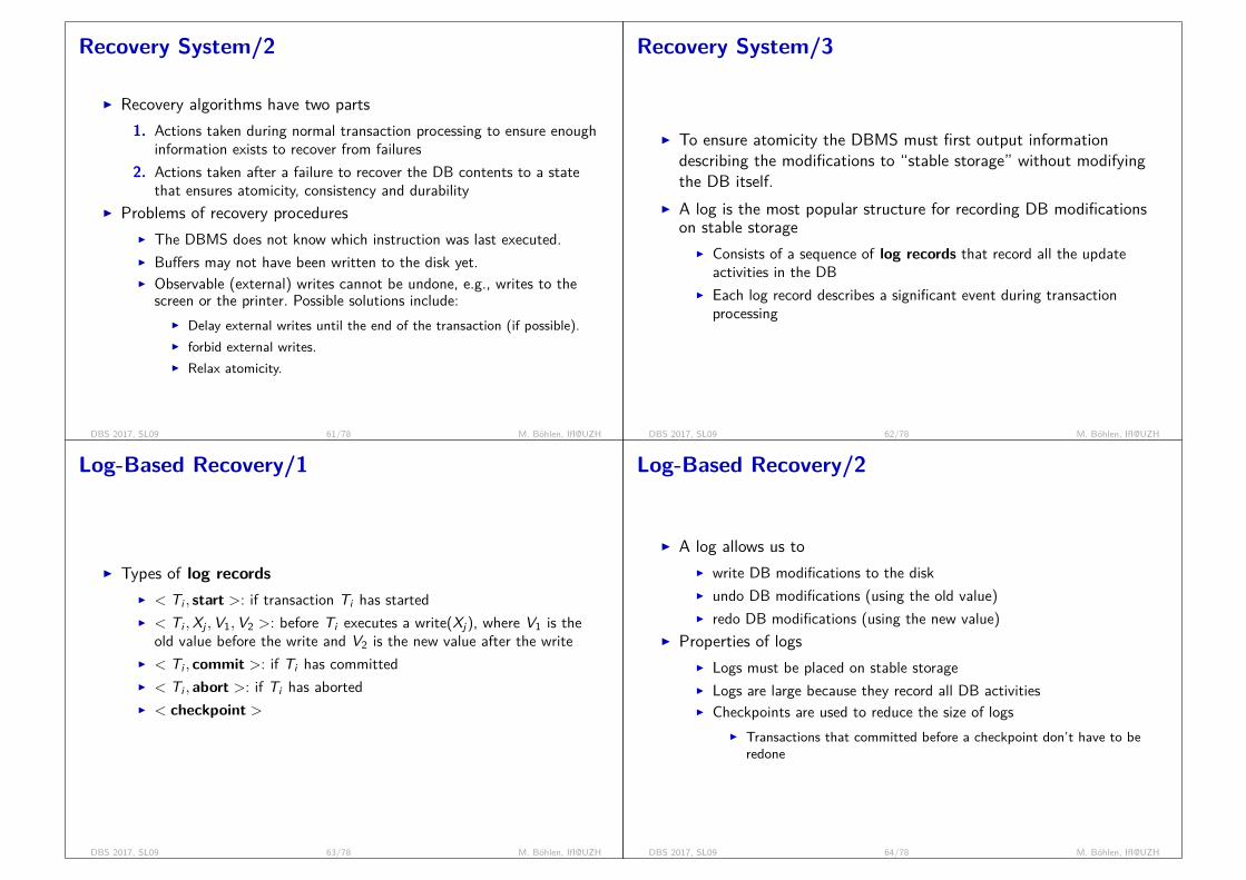
Recovery System/2
I Recovery algorithms have two parts1. Actions taken during normal transaction processing to ensure enough
information exists to recover from failures2. Actions taken after a failure to recover the DB contents to a state
that ensures atomicity, consistency and durabilityI Problems of recovery procedures
I The DBMS does not know which instruction was last executed.I Buffers may not have been written to the disk yet.I Observable (external) writes cannot be undone, e.g., writes to the
screen or the printer. Possible solutions include:I Delay external writes until the end of the transaction (if possible).I forbid external writes.I Relax atomicity.
DBS 2017, SL09 61/78 M. Böhlen, IfI@UZH
Recovery System/3
I To ensure atomicity the DBMS must first output informationdescribing the modifications to “stable storage” without modifyingthe DB itself.
I A log is the most popular structure for recording DB modificationson stable storage
I Consists of a sequence of log records that record all the updateactivities in the DB
I Each log record describes a significant event during transactionprocessing
DBS 2017, SL09 62/78 M. Böhlen, IfI@UZH
Log-Based Recovery/1
I Types of log recordsI < Ti , start >: if transaction Ti has startedI < Ti ,Xj ,V1,V2 >: before Ti executes a write(Xj), where V1 is the
old value before the write and V2 is the new value after the writeI < Ti , commit >: if Ti has committedI < Ti , abort >: if Ti has abortedI < checkpoint >
DBS 2017, SL09 63/78 M. Böhlen, IfI@UZH
Log-Based Recovery/2
I A log allows us toI write DB modifications to the diskI undo DB modifications (using the old value)I redo DB modifications (using the new value)
I Properties of logsI Logs must be placed on stable storageI Logs are large because they record all DB activitiesI Checkpoints are used to reduce the size of logs
I Transactions that committed before a checkpoint don’t have to beredone
DBS 2017, SL09 64/78 M. Böhlen, IfI@UZH
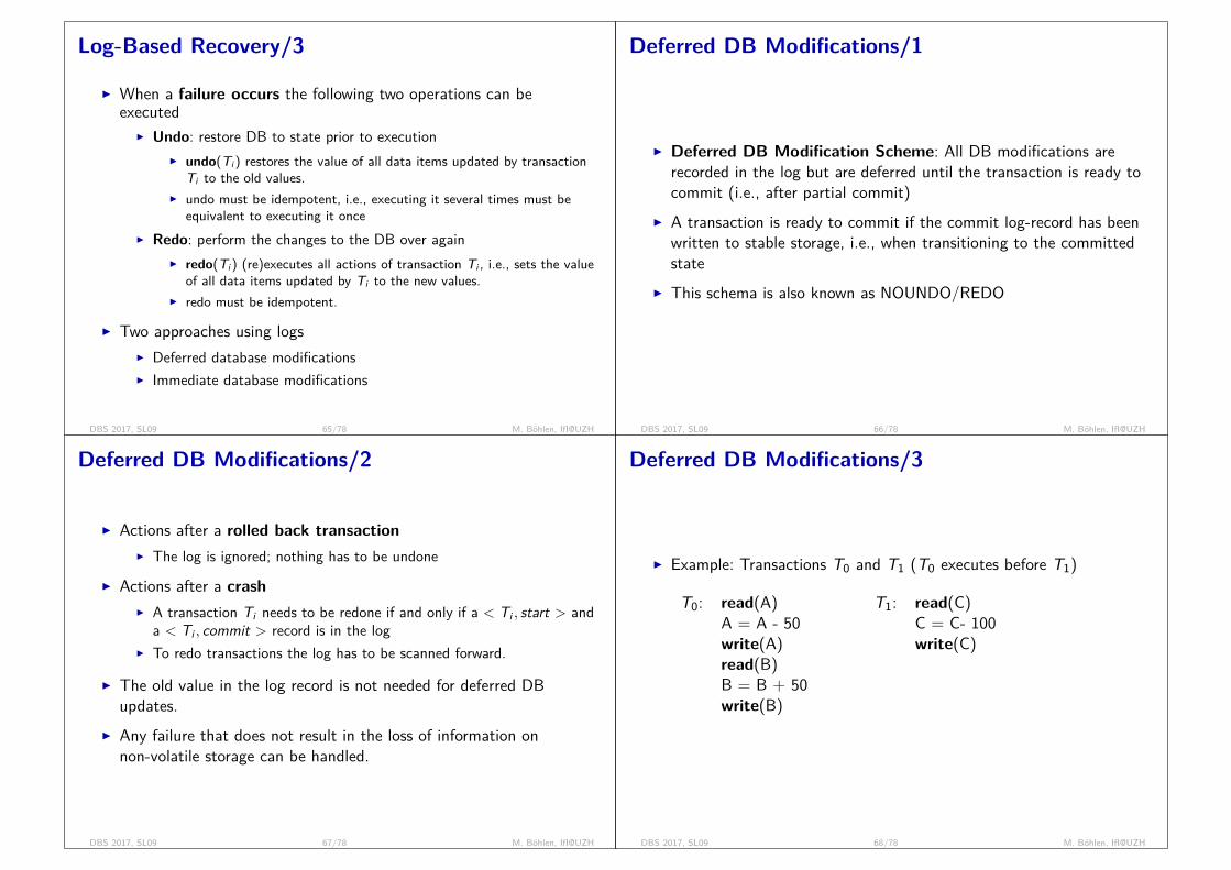
Log-Based Recovery/3
I When a failure occurs the following two operations can beexecuted
I Undo: restore DB to state prior to executionI undo(Ti ) restores the value of all data items updated by transaction
Ti to the old values.I undo must be idempotent, i.e., executing it several times must be
equivalent to executing it onceI Redo: perform the changes to the DB over again
I redo(Ti ) (re)executes all actions of transaction Ti , i.e., sets the valueof all data items updated by Ti to the new values.
I redo must be idempotent.
I Two approaches using logsI Deferred database modificationsI Immediate database modifications
DBS 2017, SL09 65/78 M. Böhlen, IfI@UZH
Deferred DB Modifications/1
I Deferred DB Modification Scheme: All DB modifications arerecorded in the log but are deferred until the transaction is ready tocommit (i.e., after partial commit)
I A transaction is ready to commit if the commit log-record has beenwritten to stable storage, i.e., when transitioning to the committedstate
I This schema is also known as NOUNDO/REDO
DBS 2017, SL09 66/78 M. Böhlen, IfI@UZH
Deferred DB Modifications/2
I Actions after a rolled back transactionI The log is ignored; nothing has to be undone
I Actions after a crashI A transaction Ti needs to be redone if and only if a < Ti , start > and
a < Ti , commit > record is in the logI To redo transactions the log has to be scanned forward.
I The old value in the log record is not needed for deferred DBupdates.
I Any failure that does not result in the loss of information onnon-volatile storage can be handled.
DBS 2017, SL09 67/78 M. Böhlen, IfI@UZH
Deferred DB Modifications/3
I Example: Transactions T0 and T1 (T0 executes before T1)
T0: read(A) T1: read(C)A = A - 50 C = C- 100write(A) write(C)read(B)B = B + 50write(B)
DBS 2017, SL09 68/78 M. Böhlen, IfI@UZH
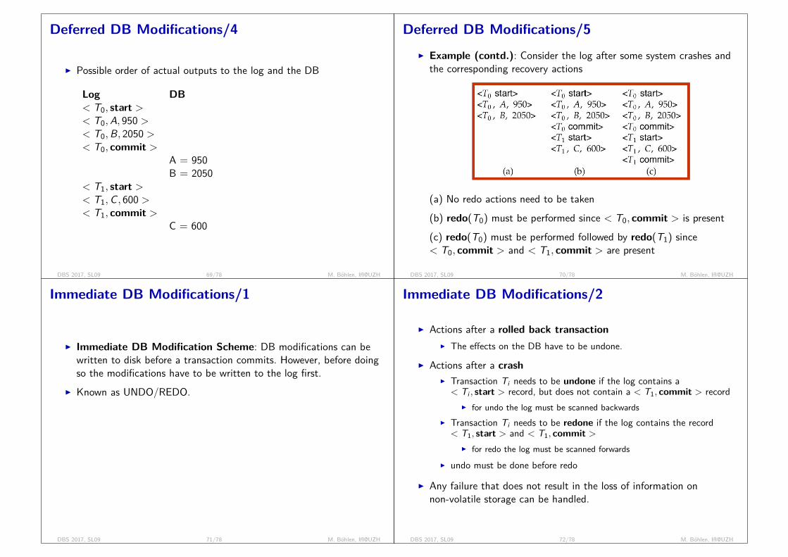
Deferred DB Modifications/4
I Possible order of actual outputs to the log and the DB
Log DB< T0, start >< T0,A, 950 >< T0,B, 2050 >< T0, commit >
A = 950B = 2050
< T1, start >< T1,C , 600 >< T1, commit >
C = 600
DBS 2017, SL09 69/78 M. Böhlen, IfI@UZH
Deferred DB Modifications/5I Example (contd.): Consider the log after some system crashes and
the corresponding recovery actions
(a) No redo actions need to be taken(b) redo(T0) must be performed since < T0, commit > is present(c) redo(T0) must be performed followed by redo(T1) since< T0, commit > and < T1, commit > are present
DBS 2017, SL09 70/78 M. Böhlen, IfI@UZH
Immediate DB Modifications/1
I Immediate DB Modification Scheme: DB modifications can bewritten to disk before a transaction commits. However, before doingso the modifications have to be written to the log first.
I Known as UNDO/REDO.
DBS 2017, SL09 71/78 M. Böhlen, IfI@UZH
Immediate DB Modifications/2
I Actions after a rolled back transactionI The effects on the DB have to be undone.
I Actions after a crashI Transaction Ti needs to be undone if the log contains a
< Ti , start > record, but does not contain a < T1, commit > recordI for undo the log must be scanned backwards
I Transaction Ti needs to be redone if the log contains the record< T1, start > and < T1, commit >
I for redo the log must be scanned forwardsI undo must be done before redo
I Any failure that does not result in the loss of information onnon-volatile storage can be handled.
DBS 2017, SL09 72/78 M. Böhlen, IfI@UZH

Immediate DB Modifications/3
I Example (contd.): Consider the log after some system crashes andthe corresponding recovery actions
(a) undo(T0): B is restored to 2000 and A to 1000(b) undo(T1) and redo(T0): C is restored to 700, and then A and Bare set to 950 and 2050, respectively(c) redo(T0) and redo(T1): A and B are set to 950 and 2050,respectively; then C is set to 600
DBS 2017, SL09 73/78 M. Böhlen, IfI@UZH
Review 9.6List advantages and disadvantages of respectively, deferred andimmediate database updates.
DBS 2017, SL09 74/78 M. Böhlen, IfI@UZH
Checkpoints/1
I Problems in recovery procedureI Searching the entire log is time-consumingI We might unnecessarily redo transactions which have already output
their updates to the DB
I Streamline recovery procedure by periodically performingcheckpointing1. Output all log records currently residing in main memory onto stable
storage.2. Output all modified buffer blocks to the disk.3. Write a log record < checkpoint > onto stable storage
I Any transaction Ti with a < T1, commit > record before a< checkpoint > record in the log need not be considered after asystem crash
DBS 2017, SL09 75/78 M. Böhlen, IfI@UZH
Checkpoints/2
I Recovery procedure: Only the most recent transaction Ti thatstarted before the checkpoint, and transactions that started after Tineed to be considered.1. Scan backwards from end of log to find the most recent
< checkpoint > record2. Continue scanning backwards till a record < Ti , start > is found.3. Need only consider the part of log following < Ti , start > record.
Earlier part of log can be ignored and can be erased.4. Scan forward the log (starting from Ti).5. For all transactions Tj with no < Tj , commit > record, execute
undo(Tj).I Done only in case of immediate modification
6. For all transactions Tj with < Tj , commit > record, executeredo(Tj).
DBS 2017, SL09 76/78 M. Böhlen, IfI@UZH
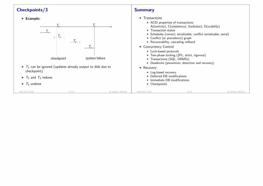
Checkpoints/3I Example:
I T1 can be ignored (updates already output to disk due tocheckpoint)
I T2 and T3 redone.I T4 undone
DBS 2017, SL09 77/78 M. Böhlen, IfI@UZH
SummaryI Transactions
I ACID properties of transactions:A(tomicity), C(onsistency), I(soltaion), D(urability)
I Transaction statesI Schedules (correct; serializable; conflict serializable; serial)I Conflict (or precedence) graphI Recoverability, cascading rollback
I Concurrency ControlI Lock-based protocolsI Two-phase locking (2PL, strict, rigorous)I Transactions (SQL, DBMSs)I Deadlocks (prevention; detection and recovery)
I RecoveryI Log-based recoveryI Deferred DB modificationsI Immediate DB modificationsI Checkpoints
DBS 2017, SL09 78/78 M. Böhlen, IfI@UZH
Database SystemsSpring 2017
1. Exam and syllabus2. DBS courses at IfI3. BSc theses, etc.4. Beyond the DBS course
DBS 2017, SL10 1/25 M. Böhlen, IfI@UZH
Exam and Syllabus
DBS 2017, SL10 2/25 M. Böhlen, IfI@UZH
The Exam
I The final exam is written and takes placeTuesday, June 20, 10:15 - 12:00 in BIN 1.B.01 and BIN 0.K.02
(see VVZ web page for details).
I Auxiliary material during exam: 1 A4 sheet with notes.
I Course web page: http://www.ifi.uzh.ch/dbtg/I The textbook is Database Systems by Elmasri and Navathe, 6th
edition.
DBS 2017, SL10 3/25 M. Böhlen, IfI@UZH
What is Important
I Being precise is important.
I Solving relevant examples is important.
I Understanding material in detail; apply to new examples.
I It is not sufficient to “know about it” or to “reproduce”.
I You must understand and apply techniques learned during thecourse.
I Exercises are representative for exam and are the best preparation.
I Simple and readable solutions are important (this has an impact onyour grade).
DBS 2017, SL10 4/25 M. Böhlen, IfI@UZH

Preparation Material
I Exercise with solutions (practice to do exercises yourself before youlook at solution)
I Lectures with reviews
I Slides
I Textbook
I Exams of the last five years (note that the material has evolved;e.g., definition of B+ tree; mapping from ER to relational DB)
I Open door policy in the database group
DBS 2017, SL10 5/25 M. Böhlen, IfI@UZH
Syllabus/1
I Relational model, algebra, and calculusI Elmasri and Navathe: chapters 3 and 6I relational modelI relational algebra (RA):σ, π, ∪, −, ×ρ, ←1, 1θ, d|><| , |><|d , d|><|d , ϑ, ÷,
I domain relational calculus (DRC), FOPL
I practice Cartesian productI practice quantifiersI move between RA, DRC, natural languageI be precise (e.g., qualified names do not exist in RA; use renaming)
DBS 2017, SL10 6/25 M. Böhlen, IfI@UZH
Syllabus/2
I SQLI Elmasri and Navathe: chapters 4 and 5I data definition language, data manipulation languageI query expressions, query specifications, orthogonalityI subqueriesI duplicatesI null valuesI logical update semantics
I practice formulation of declarative queriesI consider effects of duplicates and NULL valuesI solve and try out SQL solutions with PostgreSQL
I important is systematic plan: input, output, modular SQL codeI avoid trial and error
I be conservative with SQL features
DBS 2017, SL10 7/25 M. Böhlen, IfI@UZH
Syllabus/3
I Constraints, triggers, views, DB programmingI Elmasri and Navathe: chapters 5, 12 and 25I views, with clauseI column constraints, table constraints, assertions, referential integrityI functions, triggers, stored proceduresI expressiveness, recursion
I know key concepts and their propertiesI know when and how to use these concepts; use as appropriate; helps
to solve specific problems or break down solutions into smaller partsI details of extended SQL syntax are not the crucial part
DBS 2017, SL10 8/25 M. Böhlen, IfI@UZH
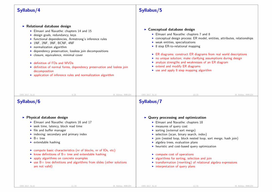
Syllabus/4
I Relational database designI Elmasri and Navathe: chapters 14 and 15I design goals, redundancy, keysI functional dependencies, Armstrong’s inference rulesI 1NF, 2NF, 3NF, BCNF, 4NFI normalization algorithmI dependency preservation, lossless join decompositionsI closure, equivalence, minimal cover
I definition of FDs and MVDsI definition of normal forms, dependency preservation and losless join
decompositionI application of inference rules and normalization algorithm
DBS 2017, SL10 9/25 M. Böhlen, IfI@UZH
Syllabus/5
I Conceptual database designI Elmasri and Navathe: chapters 7 and 8I conceptual design process: ER model, entities, attributes, relationshipsI weak entities, specializationsI 8 step ER-to-relational mapping
I ER diagrams: construct ER diagrams from real world descriptionsI no unique solution; make clarifying assumptions during designI analyze strengths and weaknesses of an ER diagramI extend and modify ER diagramsI use and apply 8 step mapping algorithm
DBS 2017, SL10 10/25 M. Böhlen, IfI@UZH
Syllabus/6
I Physical database designI Elmasri and Navathe: chapters 16 and 17I seek time, latency, block read timeI file and buffer managerI indexing: secondary and primary indexI B+ treeI extendable hashing
I compute basic characteristics (nr of blocks, nr of IOs, etc)I know definitions of B+ tree and extendable hashingI apply algorithms on concrete examplesI use B+ tree definitions and algorithms from slides (other solutions
are not valid)
DBS 2017, SL10 11/25 M. Böhlen, IfI@UZH
Syllabus/7
I Query processing and optimizationI Elmasri and Navathe: chapters 18I measures of query costI sorting (external sort merge)I selection (scan, binary search, index)I join (nested loop, block nested loop, sort merge, hash join)I algebra trees, evaluation plansI heuristic and cost-based query optimization
I compute cost of operationsI algorithms for sorting, selection and joinI transformation (rewriting) of relational algebra expressionsI interpretation of query plans
DBS 2017, SL10 12/25 M. Böhlen, IfI@UZH

Syllabus/7
I Transaction processingI Elmasri and Navathe: chapters 20, 21, 22I transactions, schedules, serializability, recoverability, ACID propertiesI concurrency control, locking, protocols, deadlocksI transactions in SQLI recovery, database log
I schedules, deadlocks, recoverabilityI conflict, conflict serializability, conflict graphsI lock-based protocols, 2PL and variantsI immediate and deferred database, redo, undo
DBS 2017, SL10 13/25 M. Böhlen, IfI@UZH
Database System Courses at IfI
DBS 2017, SL10 14/25 M. Böhlen, IfI@UZH
Database Systems Courses @IfI
I Database Systems, Spring (sem4)I Praktikum Datenbanksysteme, Fall (sem5)I Distributed Databases, Fall (sem5)I Seminar in Database Systems, Spring (sem6, sem8, sem12)I XML and Databases, Spring (sem8, sem6)I Data Warehousing, Spring (sem8, sem6; even years only)I Nonstandard Databases, Fall (sem9, sem7)
I BSc thesis, MSc thesis, independent studies (Vertiefung,Facharbeit, etc)
DBS 2017, SL10 15/25 M. Böhlen, IfI@UZH
Andreas Geppert: Praktikum Datenbanksysteme
I Since 2016 Andreas Geppert is with SwissRe.I From 2001 until 2016 Andreas Geppert was with
Credit Suisse (as database architect).I Before this he was a senior researcher in the
Database Technology Research Group.I He received his diploma in Computer Science from the University of
Karlsruhe (Germany) in 1989 and his PhD in computer science fromthe University of Zurich (1994).
I From August 1998 to August 1999 he was a visiting scientist at theIBM Almaden Research Center.
I Praktikum DatenbanksystemeI Apply/practice your SQL knowledge on a case studyI Dienstag 16:00 - 18:00
DBS 2017, SL10 16/25 M. Böhlen, IfI@UZH
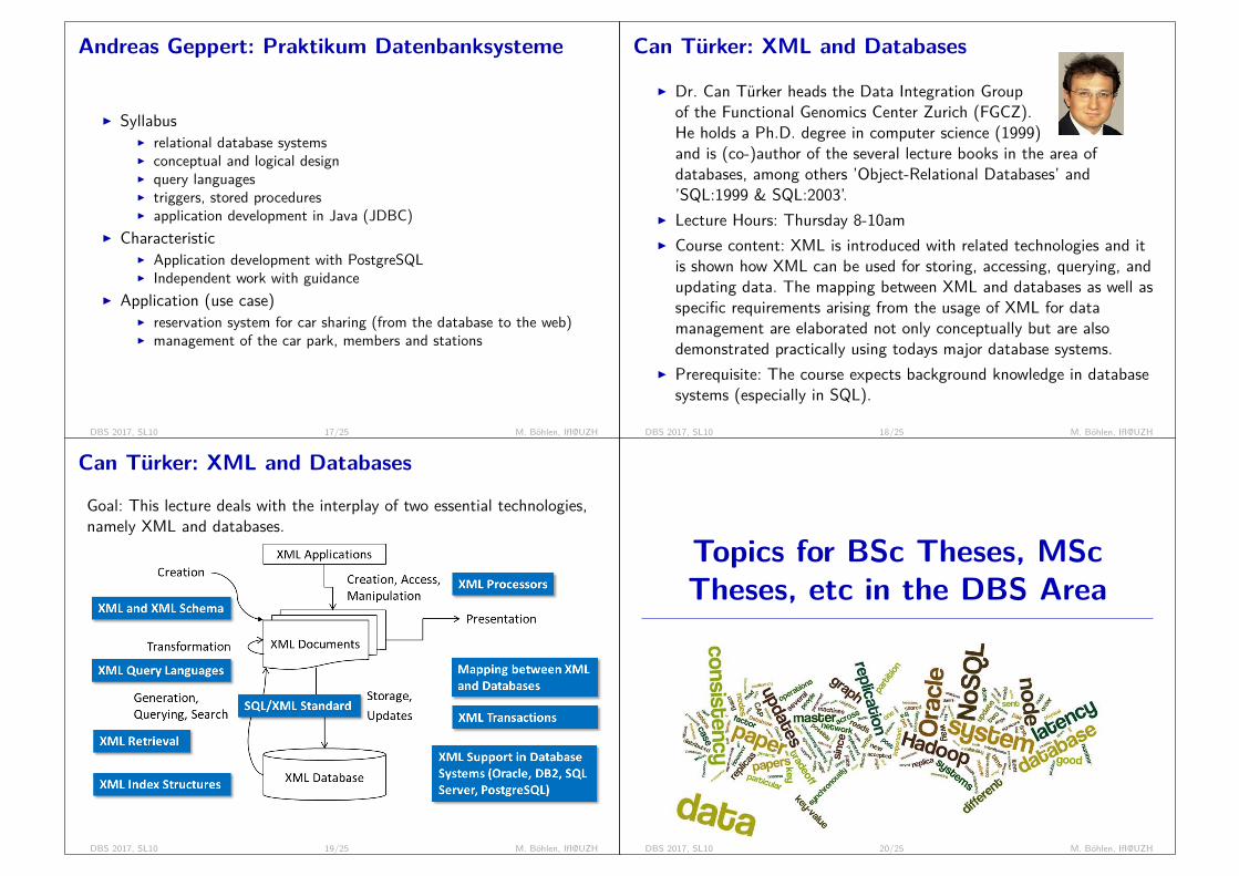
Andreas Geppert: Praktikum Datenbanksysteme
I SyllabusI relational database systemsI conceptual and logical designI query languagesI triggers, stored proceduresI application development in Java (JDBC)
I CharacteristicI Application development with PostgreSQLI Independent work with guidance
I Application (use case)I reservation system for car sharing (from the database to the web)I management of the car park, members and stations
DBS 2017, SL10 17/25 M. Böhlen, IfI@UZH
Can Türker: XML and Databases
I Dr. Can Türker heads the Data Integration Groupof the Functional Genomics Center Zurich (FGCZ).He holds a Ph.D. degree in computer science (1999)and is (co-)author of the several lecture books in the area ofdatabases, among others ’Object-Relational Databases’ and’SQL:1999 & SQL:2003’.
I Lecture Hours: Thursday 8-10amI Course content: XML is introduced with related technologies and it
is shown how XML can be used for storing, accessing, querying, andupdating data. The mapping between XML and databases as well asspecific requirements arising from the usage of XML for datamanagement are elaborated not only conceptually but are alsodemonstrated practically using todays major database systems.
I Prerequisite: The course expects background knowledge in databasesystems (especially in SQL).
DBS 2017, SL10 18/25 M. Böhlen, IfI@UZH
Can Türker: XML and Databases
Goal: This lecture deals with the interplay of two essential technologies,namely XML and databases.
DBS 2017, SL10 19/25 M. Böhlen, IfI@UZH
Topics for BSc Theses, MScTheses, etc in the DBS Area
DBS 2017, SL10 20/25 M. Böhlen, IfI@UZH

BSc and MSc Theses in the DBS AreaI We are happy to supervise BSc and MSc theses in the DBS areaI Relevant for all specializations and degreesI Typically close interaction with an assistant with weekly meetingsI Algorithms, software development, scientific writing
I Extension of PostgreSQL (parser, analyzer, query optimizer)I Incorporation of a load balancing algorithm into Apache HadoopI Work with real world data (e.g., feedbase.ch)I Matrix factorization
I Work goes into detailsI Contact assistant by email and ask for a meeting to discuss theses
DBS 2017, SL10 21/25 M. Böhlen, IfI@UZH
Beyond the DBS Course
DBS 2017, SL10 22/25 M. Böhlen, IfI@UZH
Beyond the DBS Course
I Jennifer Widom’s (Stanford) recipe for database research:1. pick a fundamental assumption underlying database systems2. drop it3. solve resulting problem
I drop: fixed structure (schema) of the dataI leads to: semistructured databases, XML databases
I drop: data sets are persistent and disk-residentI leads to: stream processing systems
I drop: tuple presence is certainI leads to: probabilistic databases
DBS 2017, SL10 23/25 M. Böhlen, IfI@UZH
Beyond the DBS Course
I drop: banking applications with short update transactionsI leads to: data warehouses, OLAP
I drop: sophisticated SQL queriesI leads to: key values stores, NoSQL
I drop: centralized processing of entire databaseI leads to: MapReduce, Hadoop
I drop: data is stored row by rowI leads to: column stores
DBS 2017, SL10 24/25 M. Böhlen, IfI@UZH