Embed Size (px)
Citation preview
Informatik fur Okonomen IIFall 2010
Database SystemsIntroduction
SL01
◮ Database Systems (5 weeks, Prof. Dr. M. Bohlen)
◮ Software Engineering (5 weeks, Prof. Dr. M. Glinz)
◮ Security (3 weeks, Prof. Dr. B. Stiller)
Inf4Oec10, SL01 1/58 M. Bohlen, ifi@uzh
Course Organization
◮ Lectures take place in KOH-B-10
◮ Time: Thursday 10:15 - 12:00
◮ Web page: https://www.csg.uzh.ch/teaching/hs10/infooekII
◮ Podcasts will be available (a few days after the lectures)
◮ Assessment: successful completion of final exam
◮ Exercises are not considered for grade (but they help you to preparefor the final exam)
◮ Exam: 20.1.2011, 10:15 - 12:00
Inf4Oec10, SL01 2/58 M. Bohlen, ifi@uzh
Exercises
◮ Information also available on course web page
◮ 5 exercises◮ 2 exercises in database systems (Amr Noureldin)◮ 2 exercises in software engineering (Reinhard Stoiber)◮ 1 exercise in security (Guilherme Machado)
◮ Download from web page
◮ Hand-in in groups is allowed
◮ No online hand-in
◮ After lecture hand-in of printed hard copy
Inf4Oec10, SL01 3/58 M. Bohlen, ifi@uzh
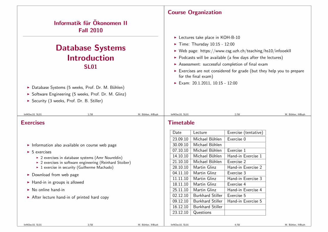
Timetable
Date Lecture Exercise (tentative)
23.09.10 Michael Bohlen Exercise 0
30.09.10 Michael Bohlen
07.10.10 Michael Bohlen Exercise 1
14.10.10 Michael Bohlen Hand-in Exercise 1
21.10.10 Michael Bohlen Exercise 2
28.10.10 Martin Glinz Hand-in Exercise 2
04.11.10 Martin Glinz Exercise 3
11.11.10 Martin Glinz Hand-in Exercise 3
18.11.10 Martin Glinz Exercise 4
25.11.10 Martin Glinz Hand-in Exercise 4
02.12.10 Burkhard Stiller Exercise 5
09.12.10 Burkhard Stiller Hand-in Exercise 5
16.12.10 Burkhard Stiller
23.12.10 Questions
Inf4Oec10, SL01 4/58 M. Bohlen, ifi@uzh
Office Hours
◮ Take place every week
◮ Office hours can be used for questions about lectures and exercises
◮ Location: RAI-D-017◮ Dates
◮ Monday 12:15 - 13:00 (Antonio Kumin)◮ Tuesday 17:15 - 18:00 (Robert Dewer, Hannes Tresch)◮ Thursday 12:30 - 13:15 (Francisco de Freitas, Jens Birchler)
Inf4Oec10, SL01 5/58 M. Bohlen, ifi@uzh
The Database System Module
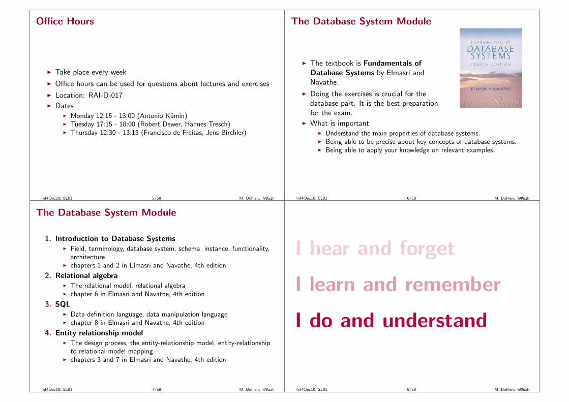
◮ The textbook is Fundamentals ofDatabase Systems by Elmasri andNavathe.
◮ Doing the exercises is crucial for thedatabase part. It is the best preparationfor the exam.
◮ What is important◮ Understand the main properties of database systems.◮ Being able to be precise about key concepts of database systems.◮ Being able to apply your knowledge on relevant examples.
Inf4Oec10, SL01 6/58 M. Bohlen, ifi@uzh
The Database System Module
1. Introduction to Database Systems◮ Field, terminology, database system, schema, instance, functionality,
architecture◮ chapters 1 and 2 in Elmasri and Navathe, 4th edition
2. Relational algebra◮ The relational model, relational algebra◮ chapter 6 in Elmasri and Navathe, 4th edition
3. SQL◮ Data definition language, data manipulation language◮ chapter 8 in Elmasri and Navathe, 4th edition
4. Entity relationship model◮ The design process, the entity-relationship model, entity-relationship
to relational model mapping◮ chapters 3 and 7 in Elmasri and Navathe, 4th edition
Inf4Oec10, SL01 7/58 M. Bohlen, ifi@uzh
I hear and forget
I learn and remember
I do and understand
Inf4Oec10, SL01 8/58 M. Bohlen, ifi@uzh
Introduction to Database Systems
◮ The database field
◮ Database and database users
◮ Basic database terminology
◮ Main characteristics of the database approach
◮ Database languages and interfaces
◮ Database system architectures
◮ History of database systems
Inf4Oec10, SL01 9/58 M. Bohlen, ifi@uzh
The Database Field/1
◮ Journal Publications◮ ACM Transaction on Database System (TODS)◮ The VLDB Journal (VLDBJ)◮ IEEE Transactions on Knowledge and Data Engineering (TKDE)◮ Information Systems (IS)
◮ Conference Publications◮ SIGMOD◮ VLDB◮ ICDE◮ EDBT
◮ DBLP Bibliography (Michael Ley, Uni Trier, Germany)◮ http://dblp.uni-trier.de/db/
◮ DBWorld mailing list◮ http://www.cs.wisc.edu/dbworld/
Inf4Oec10, SL01 10/58 M. Bohlen, ifi@uzh
The Database Field/2
Inf4Oec10, SL01 11/58 M. Bohlen, ifi@uzh
The Database Database Field/3
◮ Commercial Products◮ Oracle◮ DB2 (IBM)◮ Microsoft SQL Server◮ Sybase◮ Ingres◮ Informix◮ PC “DBMSs”: Paradox, Access, ...◮ ...
◮ Open Source Products◮ PostgreSQL◮ MySQL◮ MonetDB◮ ...
We will use MySQL for this course.
Inf4Oec10, SL01 12/58 M. Bohlen, ifi@uzh
Typical Activities of Database People
◮ Data modeling
◮ Handling large volumes of complex data
◮ Distributed databases
◮ Design of migration strategies
◮ User interface design
◮ Development of algorithms
◮ Design of languages◮ New data models and systems
◮ XML/semi-structured databases◮ Stream data processing◮ Temporal and spatial databases◮ GIS systems
Inf4Oec10, SL01 13/58 M. Bohlen, ifi@uzh
Basic Definitions/1
About, data, information, and knowledge:
◮ Data are facts that can be recorded:◮ book(Lord of the Rings, 3, 10)
◮ Information = data + meaning◮ book:
◮ title = Lord of the rings,◮ volume nr = 3,◮ price in USD = 10
◮ Knowledge = information + application
Inf4Oec10, SL01 14/58 M. Bohlen, ifi@uzh
Basic Definitions/2
◮ Mini-world: The part of the real world we are interested in
◮ Data: Known facts about the mini-world that can be recorded
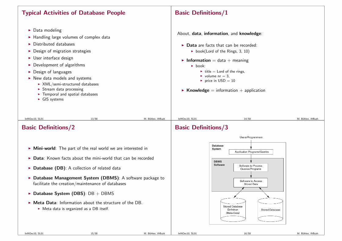
◮ Database (DB): A collection of related data
◮ Database Management System (DBMS): A software package tofacilitate the creation/maintenance of databases
◮ Database System (DBS): DB + DBMS
◮ Meta Data: Information about the structure of the DB.◮ Meta data is organized as a DB itself.
Inf4Oec10, SL01 15/58 M. Bohlen, ifi@uzh
Basic Definitions/3
Inf4Oec10, SL01 16/58 M. Bohlen, ifi@uzh

Basic Definitions/4
◮ A DBMS provides two kind of languages
◮ A data definition language (DDL) for specifying the databaseschema
◮ the database schema is stored in the data dictionary◮ the content of data dictionary is called metadata
◮ A data manipulation language (DML) for updating and queryingdatabases, i.e.,
◮ retrieval of information◮ insertion of new information◮ deletion of information◮ modification of information
◮ The standard language for database systems is SQL; “Intergalacticdata speak” [Michael Stonebraker].
◮ SQL offers a DDL and DML.
Inf4Oec10, SL01 17/58 M. Bohlen, ifi@uzh
Database Applications
◮ Traditional Applications◮ Numeric and Textual Databases
◮ More Recent Applications:◮ Multimedia Databases◮ Geographic Information Systems (GIS)◮ Data Warehouses◮ Real-time and Active Databases◮ Many other applications
◮ Examples:◮ Bank (accounts)◮ Stores (inventory, sales)◮ Reservation systems◮ University (students, courses, rooms)◮ online sales (amazon.com)◮ online newspapers (nzz.ch)
Inf4Oec10, SL01 18/58 M. Bohlen, ifi@uzh
Typical DBMS Functionality/1
◮ Define a particular database in terms of its data types, structures,and constraints
◮ Construct or load the initial database contents on a secondarystorage medium
◮ Manipulating the database:◮ Retrieval: Querying, generating reports◮ Modification: Insertions, deletions and updates to its content◮ Accessing the database through Web applications
◮ Sharing by a set of concurrent users and application programswhile, at the same time, keeping all data valid and consistent
Inf4Oec10, SL01 19/58 M. Bohlen, ifi@uzh
Typical DBMS Functionality/2
◮ Other features of DBMSs:◮ Protection or security measures to prevent unauthorized access
◮ Active processing to take internal actions on data
◮ Presentation and visualization of data
◮ Maintaining the database and associated programs over the lifetimeof the database application (called database, software, and systemmaintenance)
Inf4Oec10, SL01 20/58 M. Bohlen, ifi@uzh

Database Users/1
Database users have very different tasks. There are those who use andcontrol the database content, and those who design, develop andmaintain database applications.
◮ Database administrators:◮ Responsible for authorizing access to the database, for coordinating
and monitoring its use, acquiring software and hardware resources,controlling its use and monitoring efficiency of operations.
◮ Database Designers:◮ Responsible to define the content, the structure, the constraints, and
functions or transactions against the database. They mustcommunicate with the end-users and understand their needs.
Inf4Oec10, SL01 21/58 M. Bohlen, ifi@uzh
Database Users/2
◮ End-users: They use the data for queries, reports and some of themupdate the database content. End-users can be categorized into:
◮ Casual: access database occasionally when needed◮ Naıve: they make up a large section of the end-user population.
◮ They use previously well-defined functions in the form of “cannedtransactions” against the database.
◮ Examples are bank-tellers or reservation clerks.
◮ Sophisticated:◮ These include business analysts, scientists, engineers, others
thoroughly familiar with the system capabilities.◮ Many use tools in the form of software packages that work closely
with the stored database.
◮ Stand-alone:◮ Mostly maintain personal databases using ready-to-use packaged
applications.◮ An example is a tax program user that creates its own internal
database or a user that maintains an address book
Inf4Oec10, SL01 22/58 M. Bohlen, ifi@uzh
Data Models
◮ Data Model:◮ A set of concepts to describe the structure of a database, the
operations for manipulating these structures, and certainconstraints that the database should obey.
◮ Data Model Structure and Constraints:◮ Different constructs are used to define the database structure◮ Constructs typically include elements (and their data types) as well
as groups of elements (e.g., entity, record, table), and relationshipsamong such groups
◮ Constraints specify some restrictions on valid data; these constraintsmust be enforced at all times
◮ Data Model Operations◮ These operations are used for specifying database retrievals and
updates by referring to the constructs of the data model.◮ Operations on the data model may include basic model operations
(e.g. generic insert, delete, update) and user-defined operations (e.g.compute student gpa, update inventory)
Inf4Oec10, SL01 23/58 M. Bohlen, ifi@uzh
Categories of Data Models
◮ Conceptual (high-level, semantic) data models:◮ Provide concepts that are close to the way many users perceive data.
(Also called entity-based or object-based data models.)
◮ Physical (low-level, internal) data models:◮ Provide concepts that describe details of how data is stored in the
computer. These are usually specified in an ad-hoc manner throughDBMS design and administration manuals
◮ Implementation (representational) data models:◮ Provide concepts that fall between the above two, used by many
commercial DBMS implementations (e.g. relational data models usedin many commercial systems).
Inf4Oec10, SL01 24/58 M. Bohlen, ifi@uzh
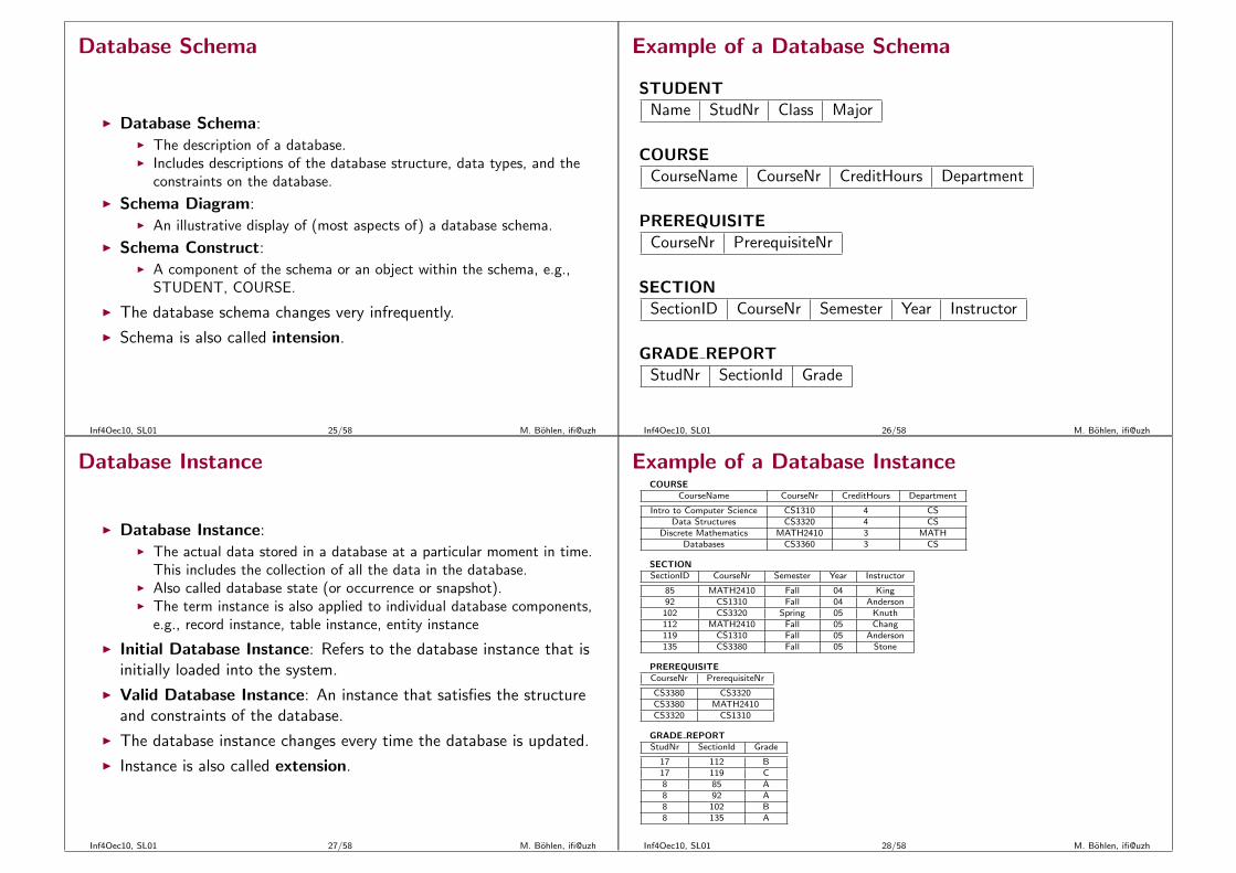
Database Schema
◮ Database Schema:◮ The description of a database.◮ Includes descriptions of the database structure, data types, and the
constraints on the database.
◮ Schema Diagram:◮ An illustrative display of (most aspects of) a database schema.
◮ Schema Construct:◮ A component of the schema or an object within the schema, e.g.,
STUDENT, COURSE.
◮ The database schema changes very infrequently.
◮ Schema is also called intension.
Inf4Oec10, SL01 25/58 M. Bohlen, ifi@uzh
Example of a Database Schema
STUDENTName StudNr Class Major
COURSECourseName CourseNr CreditHours Department
PREREQUISITECourseNr PrerequisiteNr
SECTIONSectionID CourseNr Semester Year Instructor
GRADE REPORTStudNr SectionId Grade
Inf4Oec10, SL01 26/58 M. Bohlen, ifi@uzh
Database Instance
◮ Database Instance:◮ The actual data stored in a database at a particular moment in time.
This includes the collection of all the data in the database.◮ Also called database state (or occurrence or snapshot).◮ The term instance is also applied to individual database components,
e.g., record instance, table instance, entity instance
◮ Initial Database Instance: Refers to the database instance that isinitially loaded into the system.
◮ Valid Database Instance: An instance that satisfies the structureand constraints of the database.
◮ The database instance changes every time the database is updated.
◮ Instance is also called extension.
Inf4Oec10, SL01 27/58 M. Bohlen, ifi@uzh
Example of a Database InstanceCOURSE
CourseName CourseNr CreditHours Department
Intro to Computer Science CS1310 4 CSData Structures CS3320 4 CS
Discrete Mathematics MATH2410 3 MATHDatabases CS3360 3 CS
SECTIONSectionID CourseNr Semester Year Instructor
85 MATH2410 Fall 04 King92 CS1310 Fall 04 Anderson102 CS3320 Spring 05 Knuth112 MATH2410 Fall 05 Chang119 CS1310 Fall 05 Anderson135 CS3380 Fall 05 Stone
PREREQUISITECourseNr PrerequisiteNr
CS3380 CS3320CS3380 MATH2410CS3320 CS1310
GRADE REPORTStudNr SectionId Grade
17 112 B17 119 C8 85 A8 92 A8 102 B8 135 A
Inf4Oec10, SL01 28/58 M. Bohlen, ifi@uzh

The ANSI/SPARC Three Schema Architecture/1
◮ Proposed to support DBMS characteristics of:◮ Data independence◮ Multiple views of the data
◮ Not explicitly used in commercial DBMS products, but has beenuseful in explaining database system organization
◮ Defines DBMS schemas at three levels:◮ Internal schema at the internal level to describe physical storage
structures and access paths (e.g indexes).◮ Typically uses a physical data model.
◮ Conceptual schema at the conceptual level to describe the structureand constraints for the whole database for a community of users.
◮ Uses a conceptual or an implementation data model.
◮ External schemas at the external level to describe the various userviews.
◮ Usually uses the same data model as the conceptual schema.
Inf4Oec10, SL01 29/58 M. Bohlen, ifi@uzh
The ANSI/SPARC Three Schema Architecture/2
◮ Mappings among schema levels are needed to transform requestsand data.
◮ Programs refer to an external schema, and are mapped by the DBMSto the internal schema for execution.
◮ Data extracted from the internal DBMS level is reformatted to matchthe user’s external view (e.g., formatting the results of an SQL queryfor display in a Web page)
Inf4Oec10, SL01 30/58 M. Bohlen, ifi@uzh
The ANSI/SPARC Three Schema Architecture/3
Inf4Oec10, SL01 31/58 M. Bohlen, ifi@uzh
Data Independence
◮ Logical Data Independence:◮ The capacity to change the conceptual schema without having to
change the external schemas and their associated applicationprograms.
◮ Physical Data Independence:◮ The capacity to change the internal schema without having to change
the conceptual schema.◮ For example, the internal schema may be changed when certain file
structures are reorganized or new indexes are created to improvedatabase performance
◮ When a schema at a lower level is changed, only the mappingsbetween this schema and higher-level schemas need to be changedin a DBMS that fully supports data independence.
◮ The higher-level schemas themselves are unchanged.◮ Hence, the application programs need not be changed since they refer
to the external schemas.
Inf4Oec10, SL01 32/58 M. Bohlen, ifi@uzh
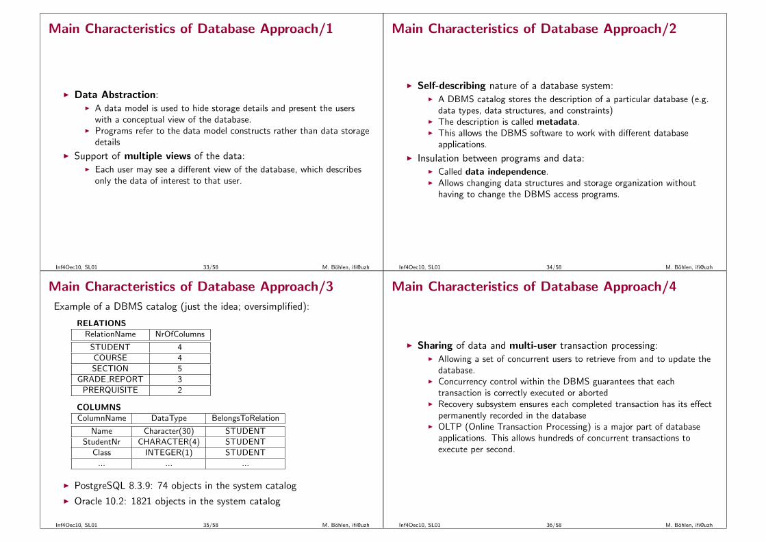
Main Characteristics of Database Approach/1
◮ Data Abstraction:◮ A data model is used to hide storage details and present the users
with a conceptual view of the database.◮ Programs refer to the data model constructs rather than data storage
details
◮ Support of multiple views of the data:◮ Each user may see a different view of the database, which describes
only the data of interest to that user.
Inf4Oec10, SL01 33/58 M. Bohlen, ifi@uzh
Main Characteristics of Database Approach/2
◮ Self-describing nature of a database system:◮ A DBMS catalog stores the description of a particular database (e.g.
data types, data structures, and constraints)◮ The description is called metadata.◮ This allows the DBMS software to work with different database
applications.
◮ Insulation between programs and data:◮ Called data independence.◮ Allows changing data structures and storage organization without
having to change the DBMS access programs.
Inf4Oec10, SL01 34/58 M. Bohlen, ifi@uzh
Main Characteristics of Database Approach/3
Example of a DBMS catalog (just the idea; oversimplified):
RELATIONSRelationName NrOfColumns
STUDENT 4
COURSE 4
SECTION 5
GRADE REPORT 3
PRERQUISITE 2
COLUMNSColumnName DataType BelongsToRelation
Name Character(30) STUDENT
StudentNr CHARACTER(4) STUDENT
Class INTEGER(1) STUDENT
... ... ...
◮ PostgreSQL 8.3.9: 74 objects in the system catalog
◮ Oracle 10.2: 1821 objects in the system catalog
Inf4Oec10, SL01 35/58 M. Bohlen, ifi@uzh
Main Characteristics of Database Approach/4
◮ Sharing of data and multi-user transaction processing:◮ Allowing a set of concurrent users to retrieve from and to update the
database.◮ Concurrency control within the DBMS guarantees that each
transaction is correctly executed or aborted◮ Recovery subsystem ensures each completed transaction has its effect
permanently recorded in the database◮ OLTP (Online Transaction Processing) is a major part of database
applications. This allows hundreds of concurrent transactions toexecute per second.
Inf4Oec10, SL01 36/58 M. Bohlen, ifi@uzh
DBMS Languages/1
◮ A DBMS offers a data definition language (DDL) and a datamanipulation language (DML)
◮ We distinguish between◮ High level or declarative languages◮ Low level or procedural languages
◮ High level or declarative language:◮ For example, the SQL relational language◮ Are set-oriented and specify what data to retrieve rather than how to
retrieve it.◮ Also called non-procedural languages.
◮ Low level or procedural language:◮ Retrieve data one record at a time;◮ Constructs such as looping are needed to retrieve multiple records,
along with positioning pointers.
Inf4Oec10, SL01 37/58 M. Bohlen, ifi@uzh
DBMS Languages/2
◮ Data Definition Language (DDL):◮ Used by the DBA and database designers to specify the conceptual
schema of a database.◮ In many DBMSs, the DDL is also used to define internal and external
schemas (views).◮ In some DBMSs, separate storage definition language (SDL) and view
definition language (VDL) are used to define internal and externalschemas.
◮ SDL is typically realized via DBMS commands provided to the DBAand database designers
Inf4Oec10, SL01 38/58 M. Bohlen, ifi@uzh
DBMS Languages/3
◮ Data Manipulation Language (DML):◮ Used to specify database retrievals and updates◮ DML commands can be embedded in a general-purpose programming
language, such as COBOL, C, C++, or Java.◮ A library of functions can also be provided to access the DBMS from
a programming language
◮ Alternatively, stand-alone DML commands can be issued directly.
Inf4Oec10, SL01 39/58 M. Bohlen, ifi@uzh
DBMS Interfaces/1
◮ Stand-alone query language interfaces◮ Example: Entering SQL queries at the DBMS interactive SQL
interface (e.g. psql in PostgreSQL, sqlplus in Oracle)
◮ Programmer interfaces for embedding DML in programminglanguages
◮ User-friendly interfaces◮ Menu-based, forms-based, graphics-based, etc.
◮ Speech as Input and Output
◮ Web Browser as an interface
◮ Parametric interfaces, e.g., bank tellers using function keys.◮ Interfaces for the DBA:
◮ Creating user accounts, granting authorizations◮ Setting system parameters◮ Changing schemas or access paths
Inf4Oec10, SL01 40/58 M. Bohlen, ifi@uzh
DBMS Interfaces/2
◮ There are various database system utilities to perform certainfunctions such as:
◮ Loading data stored in files into a database. Includes data conversiontools.
◮ Backing up the database periodically on tape.◮ Reorganizing database file structures.◮ Report generation utilities.◮ Performance monitoring utilities.◮ Other functions, such as sorting, user monitoring, data compression,
etc.
Inf4Oec10, SL01 41/58 M. Bohlen, ifi@uzh
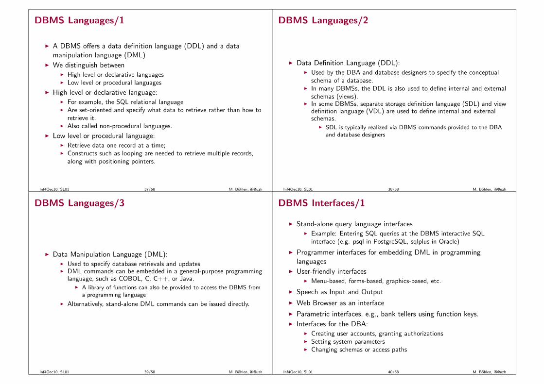
Components of the DBS Architecture
Inf4Oec10, SL01 42/58 M. Bohlen, ifi@uzh
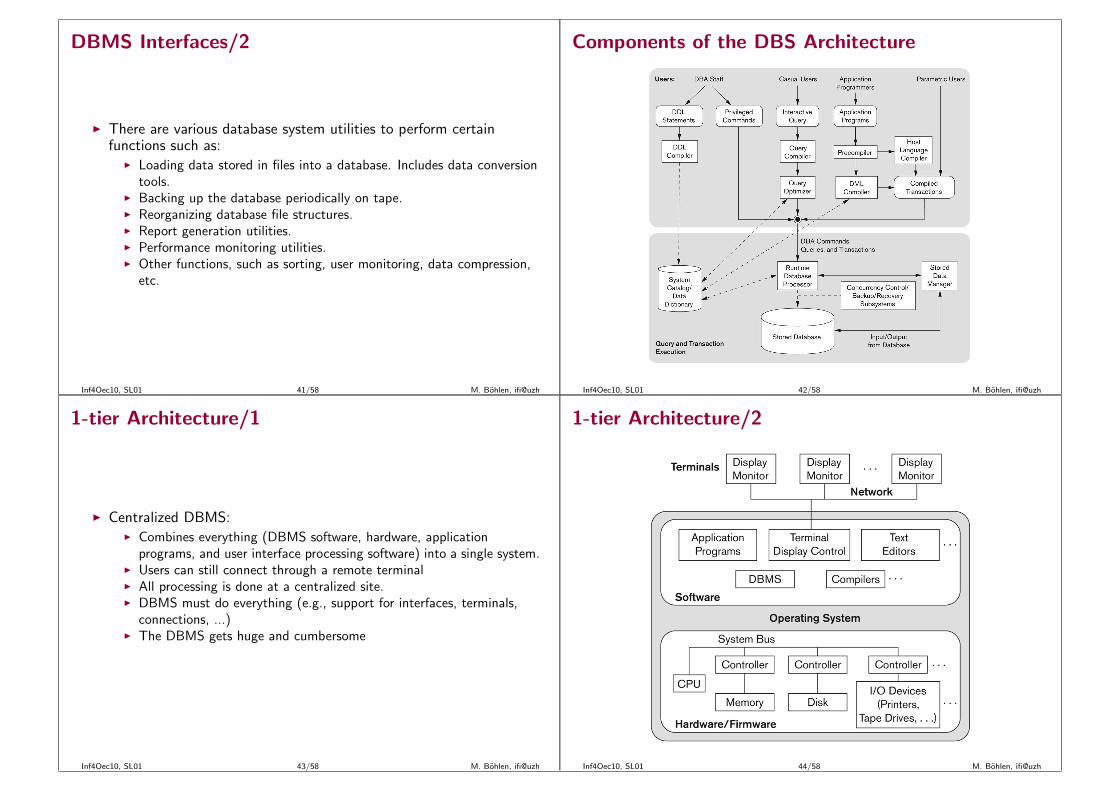
1-tier Architecture/1
◮ Centralized DBMS:◮ Combines everything (DBMS software, hardware, application
programs, and user interface processing software) into a single system.◮ Users can still connect through a remote terminal◮ All processing is done at a centralized site.◮ DBMS must do everything (e.g., support for interfaces, terminals,
connections, ...)◮ The DBMS gets huge and cumbersome
Inf4Oec10, SL01 43/58 M. Bohlen, ifi@uzh
1-tier Architecture/2
Inf4Oec10, SL01 44/58 M. Bohlen, ifi@uzh

2-tier Architecture/1
◮ Specialized Servers with Specialized functions◮ Print server◮ File server◮ DBMS server◮ Web server◮ Email server
◮ Clients can access the specialized servers as needed
Inf4Oec10, SL01 45/58 M. Bohlen, ifi@uzh
2-tier Architecture/2
◮ Clients:◮ Provide appropriate interfaces through a client software module to
access and utilize the various server resources.◮ Clients may be diskless machines or PCs or Workstations with disks
with only the client software installed.◮ Connected to the servers via some form of a network. (local area
network, wireless network, etc.)
◮ DBMS Server:◮ Provides database query and transaction services to the clients◮ Relational DBMS servers are often called SQL servers, query servers,
or transaction servers◮ Applications running on clients utilize an application program
interface (API) to access server databases via standard interfaces:◮ ODBC: Open Database Connectivity standard◮ JDBC: for Java programming access
◮ Client and server must install appropriate client module and servermodule software for ODBC or JDBC
Inf4Oec10, SL01 46/58 M. Bohlen, ifi@uzh
3-tier Architecture/1
◮ Common for web applications◮ Intermediate layer called application server or web server:
◮ Stores the web connectivity software and the business logic part ofthe application used to access the corresponding data from thedatabase server
◮ Acts like a conduit for sending partially processed data between thedatabase server and the client.
◮ Three-tier architecture can enhance security:◮ Database server only accessible via middle tier◮ Clients cannot directly access database server
Inf4Oec10, SL01 47/58 M. Bohlen, ifi@uzh
3-tier Architecture/2
Inf4Oec10, SL01 48/58 M. Bohlen, ifi@uzh
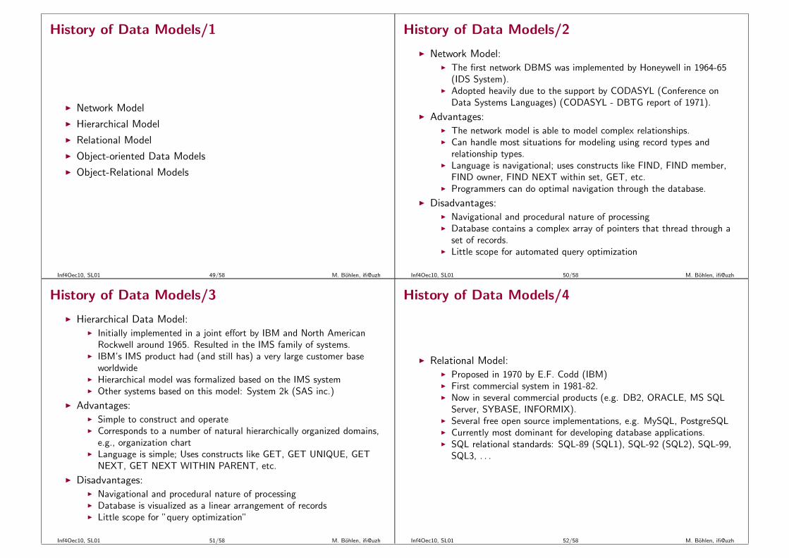
History of Data Models/1
◮ Network Model
◮ Hierarchical Model
◮ Relational Model
◮ Object-oriented Data Models
◮ Object-Relational Models
Inf4Oec10, SL01 49/58 M. Bohlen, ifi@uzh
History of Data Models/2
◮ Network Model:◮ The first network DBMS was implemented by Honeywell in 1964-65
(IDS System).◮ Adopted heavily due to the support by CODASYL (Conference on
Data Systems Languages) (CODASYL - DBTG report of 1971).
◮ Advantages:◮ The network model is able to model complex relationships.◮ Can handle most situations for modeling using record types and
relationship types.◮ Language is navigational; uses constructs like FIND, FIND member,
FIND owner, FIND NEXT within set, GET, etc.◮ Programmers can do optimal navigation through the database.
◮ Disadvantages:◮ Navigational and procedural nature of processing◮ Database contains a complex array of pointers that thread through a
set of records.◮ Little scope for automated query optimization
Inf4Oec10, SL01 50/58 M. Bohlen, ifi@uzh
History of Data Models/3
◮ Hierarchical Data Model:◮ Initially implemented in a joint effort by IBM and North American
Rockwell around 1965. Resulted in the IMS family of systems.◮ IBM’s IMS product had (and still has) a very large customer base
worldwide◮ Hierarchical model was formalized based on the IMS system◮ Other systems based on this model: System 2k (SAS inc.)
◮ Advantages:◮ Simple to construct and operate◮ Corresponds to a number of natural hierarchically organized domains,
e.g., organization chart◮ Language is simple; Uses constructs like GET, GET UNIQUE, GET
NEXT, GET NEXT WITHIN PARENT, etc.
◮ Disadvantages:◮ Navigational and procedural nature of processing◮ Database is visualized as a linear arrangement of records◮ Little scope for ”query optimization”
Inf4Oec10, SL01 51/58 M. Bohlen, ifi@uzh
History of Data Models/4
◮ Relational Model:◮ Proposed in 1970 by E.F. Codd (IBM)◮ First commercial system in 1981-82.◮ Now in several commercial products (e.g. DB2, ORACLE, MS SQL
Server, SYBASE, INFORMIX).◮ Several free open source implementations, e.g. MySQL, PostgreSQL◮ Currently most dominant for developing database applications.◮ SQL relational standards: SQL-89 (SQL1), SQL-92 (SQL2), SQL-99,
SQL3, . . .
Inf4Oec10, SL01 52/58 M. Bohlen, ifi@uzh
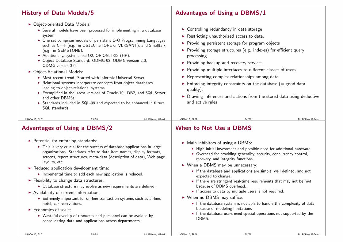
History of Data Models/5
◮ Object-oriented Data Models:◮ Several models have been proposed for implementing in a database
system.◮ One set comprises models of persistent O-O Programming Languages
such as C++ (e.g., in OBJECTSTORE or VERSANT), and Smalltalk(e.g., in GEMSTONE).
◮ Additionally, systems like O2, ORION, IRIS (HP).◮ Object Database Standard: ODMG-93, ODMG-version 2.0,
ODMG-version 3.0.
◮ Object-Relational Models:◮ Most recent trend. Started with Informix Universal Server.◮ Relational systems incorporate concepts from object databases
leading to object-relational systems.◮ Exemplified in the latest versions of Oracle-10i, DB2, and SQL Server
and other DBMSs.◮ Standards included in SQL-99 and expected to be enhanced in future
SQL standards.
Inf4Oec10, SL01 53/58 M. Bohlen, ifi@uzh
Advantages of Using a DBMS/1
◮ Controlling redundancy in data storage
◮ Restricting unauthorized access to data.
◮ Providing persistent storage for program objects
◮ Providing storage structures (e.g. indexes) for efficient queryprocessing
◮ Providing backup and recovery services.
◮ Providing multiple interfaces to different classes of users.
◮ Representing complex relationships among data.
◮ Enforcing integrity constraints on the database (= good dataquality).
◮ Drawing inferences and actions from the stored data using deductiveand active rules
Inf4Oec10, SL01 54/58 M. Bohlen, ifi@uzh
Advantages of Using a DBMS/2
◮ Potential for enforcing standards:◮ This is very crucial for the success of database applications in large
organizations. Standards refer to data item names, display formats,screens, report structures, meta-data (description of data), Web pagelayouts, etc.
◮ Reduced application development time:◮ Incremental time to add each new application is reduced.
◮ Flexibility to change data structures:◮ Database structure may evolve as new requirements are defined.
◮ Availability of current information:◮ Extremely important for on-line transaction systems such as airline,
hotel, car reservations.
◮ Economies of scale:◮ Wasteful overlap of resources and personnel can be avoided by
consolidating data and applications across departments.
Inf4Oec10, SL01 55/58 M. Bohlen, ifi@uzh
When to Not Use a DBMS
◮ Main inhibitors of using a DBMS:◮ High initial investment and possible need for additional hardware.◮ Overhead for providing generality, security, concurrency control,
recovery, and integrity functions.
◮ When a DBMS may be unnecessary:◮ If the database and applications are simple, well defined, and not
expected to change.◮ If there are stringent real-time requirements that may not be met
because of DBMS overhead.◮ If access to data by multiple users is not required.
◮ When no DBMS may suffice:◮ If the database system is not able to handle the complexity of data
because of modeling limitations◮ If the database users need special operations not supported by the
DBMS.
Inf4Oec10, SL01 56/58 M. Bohlen, ifi@uzh
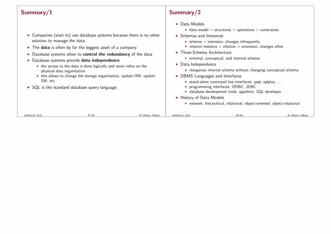
Summary/1
◮ Companies (start to) use database systems because there is no othersolution to manage the data.
◮ The data is often by far the biggest asset of a company.
◮ Database systems allow to control the redundancy of the data.◮ Database systems provide data independence
◮ the access to the data is done logically and never relies on thephysical data organization
◮ this allows to change the storage organization, update HW, updateSW, etc
◮ SQL is the standard database query language.
Inf4Oec10, SL01 57/58 M. Bohlen, ifi@uzh
Summary/2
◮ Data Models◮ data model = structures + operations + constraints
◮ Schemas and Instances◮ schema = intension; changes infrequently◮ relation instance = relation = extension; changes often
◮ Three-Schema Architecture◮ external, conceptual, and internal schema
◮ Data Independence◮ reorganize internal schema without changing conceptual schema
◮ DBMS Languages and Interfaces◮ stand-alone command line interfaces: psql, sqlplus, ...◮ programming interfaces: ODBC, JDBC◮ database development tools: pgadmin, SQL developer
◮ History of Data Models◮ network, hierarchical, relational, object-oriented, object-relational
Inf4Oec10, SL01 58/58 M. Bohlen, ifi@uzh

Informatik fur Okonomen IIFall 2010
Database SystemsRelational Algebra
SL02
◮ The Relational Model
◮ Basic Relational Algebra Operators: σ, π,∪,×,−, ρ◮ Additional Relational Algebra Operators: ∩,1,←
Inf4Oec10, SL02 1/48 M. Bohlen, ifi@uzh
The Relational Model
◮ Attribute, domain, tuple, relation, database
◮ Instance, schema
◮ Key constraints, entity constraints, foreign key
Inf4Oec10, SL02 2/48 M. Bohlen, ifi@uzh
The Relational Model
◮ The relational model is based on the concept of a relation.
◮ A relation is a mathematical concept based on the ideas of sets.◮ The relational model was proposed by Codd from IBM Research in
the paper:◮ A Relational Model for Large Shared Data Banks, Communications of
the ACM, June 1970
◮ The above paper caused a major revolution in the field of databasemanagement and earned Codd the coveted ACM Turing Award.
◮ The strength of the relational approach comes from the formalfoundation provided by the theory of relations.
◮ In practice, there is a standard model based on SQL. There areseveral important differences between the formal model and thepractical model, as we shall see.
Inf4Oec10, SL02 3/48 M. Bohlen, ifi@uzh
Relation Schema
◮ R(A1,A2, . . . ,An) is a relation schema
◮ R is the name of the relation.
◮ A1,A2, . . . ,An are attributes
◮ Example:Customer(CustName,CustStreet,CustCity)
Inf4Oec10, SL02 4/48 M. Bohlen, ifi@uzh
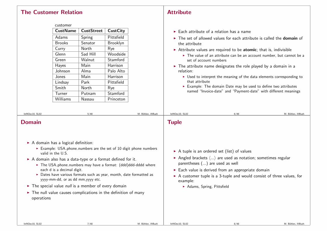
The Customer Relation
customer
CustName CustStreet CustCity
Adams Spring Pittsfield
Brooks Senator Brooklyn
Curry North Rye
Glenn Sad Hill Woodside
Green Walnut Stamford
Hayes Main Harrison
Johnson Alma Palo Alto
Jones Main Harrison
Lindsay Park Pittsfield
Smith North Rye
Turner Putnam Stamford
Williams Nassau Princeton
Inf4Oec10, SL02 5/48 M. Bohlen, ifi@uzh
Attribute
◮ Each attribute of a relation has a name
◮ The set of allowed values for each attribute is called the domain ofthe attribute
◮ Attribute values are required to be atomic; that is, indivisible◮ The value of an attribute can be an account number, but cannot be a
set of account numbers
◮ The attribute name designates the role played by a domain in arelation:
◮ Used to interpret the meaning of the data elements corresponding tothat attribute
◮ Example: The domain Date may be used to define two attributesnamed “Invoice-date” and “Payment-date” with different meanings
Inf4Oec10, SL02 6/48 M. Bohlen, ifi@uzh
Domain
◮ A domain has a logical definition:◮ Example: USA phone numbers are the set of 10 digit phone numbers
valid in the U.S.
◮ A domain also has a data-type or a format defined for it.◮ The USA phone numbers may have a format: (ddd)ddd-dddd where
each d is a decimal digit.◮ Dates have various formats such as year, month, date formatted as
yyyy-mm-dd, or as dd mm,yyyy etc.
◮ The special value null is a member of every domain
◮ The null value causes complications in the definition of manyoperations
Inf4Oec10, SL02 7/48 M. Bohlen, ifi@uzh
Tuple
◮ A tuple is an ordered set (list) of values
◮ Angled brackets 〈...〉 are used as notation; sometimes regularparentheses (...) are used as well
◮ Each value is derived from an appropriate domain◮ A customer tuple is a 3-tuple and would consist of three values, for
example:◮ Adams, Spring, Pittsfield
Inf4Oec10, SL02 8/48 M. Bohlen, ifi@uzh
Relational Instance
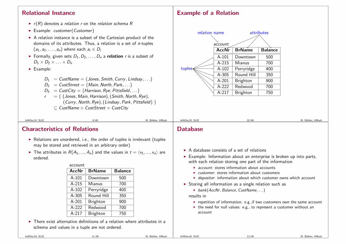
◮ r(R) denotes a relation r on the relation schema R
◮ Example: customer(Customer)
◮ A relation instance is a subset of the Cartesian product of thedomains of its attributes. Thus, a relation is a set of n-tuples(a1, a2, . . . , an) where each ai ∈ Di
◮ Formally, given sets D1,D2, . . . ,Dn a relation r is a subset ofD1 × D2 × . . .× Dn
◮ Example:
D1 = CustName = {Jones, Smith,Curry , Lindsay , . . .}D2 = CustStreet = {Main,North,Park , . . .}D3 = CustCity = {Harrison,Rye,Pittsfield , . . .}r = { (Jones,Main,Harrison), (Smith,North,Rye),
(Curry ,North,Rye), (Lindsay ,Park ,Pittsfield) }⊆ CustName × CustStreet × CustCity
Inf4Oec10, SL02 9/48 M. Bohlen, ifi@uzh
Example of a Relation
relation name
tuples
attributes
account
AccNr BrName Balance
A-101 Downtown 500
A-215 Mianus 700
A-102 Perryridge 400
A-305 Round Hill 350
A-201 Brighton 900
A-222 Redwood 700
A-217 Brighton 750
Inf4Oec10, SL02 10/48 M. Bohlen, ifi@uzh
Characteristics of Relations
◮ Relations are unordered, i.e., the order of tuples is irrelevant (tuplesmay be stored and retrieved in an arbitrary order)
◮ The attributes in R(A1, ...,An) and the values in t = 〈v1, ..., vn〉 areordered.
account
AccNr BrName Balance
A-101 Downtown 500
A-215 Mianus 700
A-102 Perryridge 400
A-305 Round Hill 350
A-201 Brighton 900
A-222 Redwood 700
A-217 Brighton 750
◮ There exist alternative definitions of a relation where attributes in aschema and values in a tuple are not ordered.
Inf4Oec10, SL02 11/48 M. Bohlen, ifi@uzh
Database
◮ A database consists of a set of relations◮ Example: Information about an enterprise is broken up into parts,
with each relation storing one part of the information◮ account: stores information about accounts◮ customer: stores information about customers◮ depositor: information about which customer owns which account
◮ Storing all information as a single relation such as◮ bank(AccNr ,Balance,CustName, . . .)
results in◮ repetition of information: e.g.,if two customers own the same account◮ the need for null values: e.g., to represent a customer without an
account
Inf4Oec10, SL02 12/48 M. Bohlen, ifi@uzh
The Depositor Relation
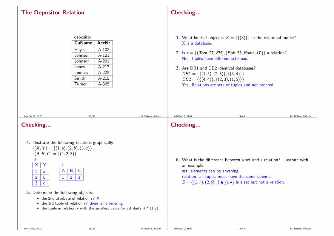
depositor
CuName AccNr
Hayes A-102
Johnson A-101
Johnson A-201
Jones A-217
Lindsay A-222
Smith A-215
Turner A-305
Inf4Oec10, SL02 13/48 M. Bohlen, ifi@uzh
Checking...
1. What kind of object is X = {{(3)}} in the relational model?X is a database.
2. Is r = {(Tom, 27,ZH), (Bob, 33,Rome, IT )} a relation?No. Tuples have different schemas.
3. Are DB1 and DB2 identical databases?DB1 = {{(1, 5), (2, 3)}, {(4, 4)}}DB2 = {{(4, 4)}, {(2, 3), (1, 5)}}Yes. Relations are sets of tuples and not ordered
Inf4Oec10, SL02 14/48 M. Bohlen, ifi@uzh
Checking...
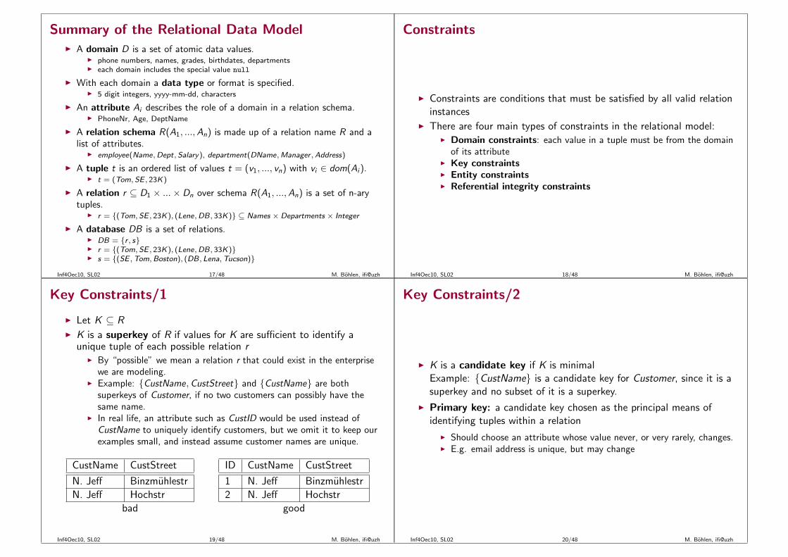
4. Illustrate the following relations graphically:r(X ,Y ) = {(1, a), (2, b), (3, c)}s(A,B ,C ) = {(1, 2, 3)}r
X Y
1 a
2 b
3 c
s
A B C
1 2 3
5. Determine the following objects:◮ the 2nd attribute of relation r? X◮ the 3rd tuple of relation r? there is no ordering◮ the tuple in relation r with the smallest value for attribute X? (1,a)
Inf4Oec10, SL02 15/48 M. Bohlen, ifi@uzh
Checking...
6. What is the difference between a set and a relation? Illustrate withan example.set: elements can be anything.relation: all tuples must have the same schema.S = {(1, r), (2, c©, {⋆}), •} is a set but not a relation.
Inf4Oec10, SL02 16/48 M. Bohlen, ifi@uzh
Summary of the Relational Data Model◮ A domain D is a set of atomic data values.
◮ phone numbers, names, grades, birthdates, departments◮ each domain includes the special value null
◮ With each domain a data type or format is specified.◮ 5 digit integers, yyyy-mm-dd, characters
◮ An attribute Ai describes the role of a domain in a relation schema.◮ PhoneNr, Age, DeptName
◮ A relation schema R(A1, ...,An) is made up of a relation name R and alist of attributes.
◮ employee(Name,Dept,Salary), department(DName,Manager ,Address)
◮ A tuple t is an ordered list of values t = (v1, ..., vn) with vi ∈ dom(Ai ).◮ t = (Tom, SE , 23K)
◮ A relation r ⊆ D1 × ...× Dn over schema R(A1, ...,An) is a set of n-arytuples.
◮ r = {(Tom, SE , 23K), (Lene,DB, 33K)} ⊆ Names × Departments × Integer
◮ A database DB is a set of relations.◮ DB = {r , s}◮ r = {(Tom, SE , 23K), (Lene,DB, 33K)}◮ s = {(SE ,Tom,Boston), (DB, Lena,Tucson)}
Inf4Oec10, SL02 17/48 M. Bohlen, ifi@uzh
Constraints
◮ Constraints are conditions that must be satisfied by all valid relationinstances
◮ There are four main types of constraints in the relational model:◮ Domain constraints: each value in a tuple must be from the domain
of its attribute◮ Key constraints◮ Entity constraints◮ Referential integrity constraints
Inf4Oec10, SL02 18/48 M. Bohlen, ifi@uzh
Key Constraints/1
◮ Let K ⊆ R◮ K is a superkey of R if values for K are sufficient to identify a
unique tuple of each possible relation r◮ By “possible” we mean a relation r that could exist in the enterprise
we are modeling.◮ Example: {CustName,CustStreet} and {CustName} are both
superkeys of Customer, if no two customers can possibly have thesame name.
◮ In real life, an attribute such as CustID would be used instead ofCustName to uniquely identify customers, but we omit it to keep ourexamples small, and instead assume customer names are unique.
CustName CustStreet
N. Jeff Binzmuhlestr
N. Jeff Hochstr
bad
ID CustName CustStreet
1 N. Jeff Binzmuhlestr
2 N. Jeff Hochstr
good
Inf4Oec10, SL02 19/48 M. Bohlen, ifi@uzh
Key Constraints/2
◮ K is a candidate key if K is minimalExample: {CustName} is a candidate key for Customer, since it is asuperkey and no subset of it is a superkey.
◮ Primary key: a candidate key chosen as the principal means ofidentifying tuples within a relation
◮ Should choose an attribute whose value never, or very rarely, changes.◮ E.g. email address is unique, but may change
Inf4Oec10, SL02 20/48 M. Bohlen, ifi@uzh

Entity Constraints
◮ The entity constraint requires that the primary key attributes ofeach relation may not have null values.
◮ The reason is that primary keys are used to identify the individualtuples.
◮ If the primary key has several attributes none of these attributevalues may be null.
◮ Other attributes of the relation may also disallow null valuesalthough they are not members of the primary key.
ID Name CustStreet
1 N. Jeff Binzmuhlestr
T. Hurd Hochstr
bad
ID Name CustStreet
1 N. Jeff Binzmuhlestr
2 T. Hurd Hochstr
good
Inf4Oec10, SL02 21/48 M. Bohlen, ifi@uzh
Referential Integrity Constraint
◮ A relation schema may have an attribute that corresponds to theprimary key of another relation. The attribute is called a foreignkey.
◮ E.g. CustName and AccNr attributes of depositor are foreign keys tocustomer and account respectively.
◮ Only values occurring in the primary key attribute of the referencedrelation (or null values) may occur in the foreign key attribute of thereferencing relation.
◮ In a graphical representation of the schema a referential integrityconstraint is often displayed as a directed arc from the foreign keyattribute to the primary key attribute.
ID CustName CStreetID
1 N. Jeff 2
2 N. Jeff 4
StreetID Street
2 Binzmuhlestr
3 Hochstr
bad (good if, e.g., 4 is replaced by 3)
Inf4Oec10, SL02 22/48 M. Bohlen, ifi@uzh
Checking...
1. Determine keys of relation R :R
X Y Z
1 2 3
1 4 5
2 2 2
X is not a keyY is not a keyZ could be a keyXY could be a key
Inf4Oec10, SL02 23/48 M. Bohlen, ifi@uzh
Query Languages
◮ Language in which user requests information from the database.
◮ Categories of languages
◮ Procedural: specifies how to do it; can be used for query optimization◮ Declarative: specifies what to do; not suitable for query optimization
◮ Pure languages:◮ Relational algebra (procedural)◮ Tuple relational calculus (declarative)◮ Domain relational calculus (declarative)
◮ Pure languages form underlying basis of query languages that peopleuse.
Inf4Oec10, SL02 24/48 M. Bohlen, ifi@uzh

The Basic Relational Algebra
◮ select σ
◮ project π
◮ union ∪◮ set difference −◮ Cartesian product ×◮ rename ρ
Inf4Oec10, SL02 25/48 M. Bohlen, ifi@uzh
Relational Algebra
◮ The relational algebra is a procedural language◮ The relational algebra consists of six basic operators
◮ select: σ◮ project: π◮ union: ∪◮ set difference: −◮ Cartesian product: ×◮ rename: ρ
◮ The operators take one or two relations as inputs and produce a newrelation as a result.
◮ This property makes the algebra closed (i.e., all objects in therelational algebra are relations).
Inf4Oec10, SL02 26/48 M. Bohlen, ifi@uzh
Select Operation
◮ Notation: σp(r)
◮ p is called the selection predicate
◮ Definition: t ∈ σp(r)⇔ t ∈ r ∧ p(t)
◮ p is a formula in propositional calculus consisting of termsconnected by : ∧ (and), ∨ (or), ¬ (not)
◮ Example: σBranchName=“Perryridge”(account)
◮ Example: σA=B∧D>5(r)r
A B C D
α α 1 7α β 5 7β β 12 3β β 23 10
σA=B∧D>5(r)
A B C D
α α 1 7β β 23 10
Inf4Oec10, SL02 27/48 M. Bohlen, ifi@uzh
Project Operation
◮ Notation: πA1,...,Ak(r)
◮ The result is defined as the relation of k columns obtained byerasing the columns that are not listed
◮ Definition: t ∈ πA1,...,Ak(r)⇔ ∃x(x ∈ r ∧ t = x [A1, . . . ,Ak ])
◮ There are no duplicate rows in the result since relations are sets
◮ Example: πAccNr ,Balance(account)
◮ Example: πA,C (r)
r
A B C
α 10 1α 20 1β 30 1β 40 2
πA,C (r)
A C
α 1β 1β 2
Inf4Oec10, SL02 28/48 M. Bohlen, ifi@uzh
Union Operation
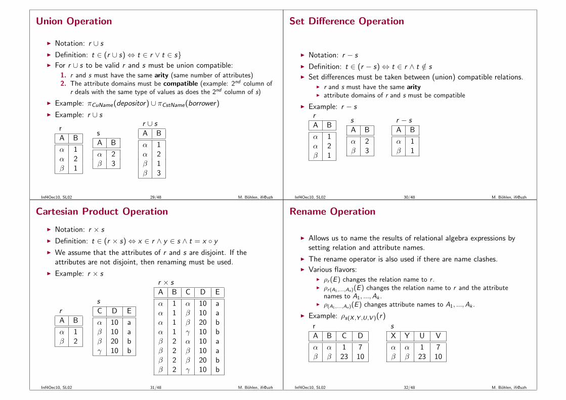
◮ Notation: r ∪ s
◮ Definition: t ∈ (r ∪ s)⇔ t ∈ r ∨ t ∈ s}◮ For r ∪ s to be valid r and s must be union compatible:
1. r and s must have the same arity (same number of attributes)2. The attribute domains must be compatible (example: 2nd column of
r deals with the same type of values as does the 2nd column of s)
◮ Example: πCuName(depositor) ∪ πCstName(borrower)
◮ Example: r ∪ s
r
A B
α 1α 2β 1
s
A B
α 2β 3
r ∪ s
A B
α 1α 2β 1β 3
Inf4Oec10, SL02 29/48 M. Bohlen, ifi@uzh
Set Difference Operation
◮ Notation: r − s
◮ Definition: t ∈ (r − s)⇔ t ∈ r ∧ t /∈ s◮ Set differences must be taken between (union) compatible relations.
◮ r and s must have the same arity◮ attribute domains of r and s must be compatible
◮ Example: r − sr
A B
α 1α 2β 1
s
A B
α 2β 3
r − s
A B
α 1β 1
Inf4Oec10, SL02 30/48 M. Bohlen, ifi@uzh
Cartesian Product Operation
◮ Notation: r × s
◮ Definition: t ∈ (r × s)⇔ x ∈ r ∧ y ∈ s ∧ t = x ◦ y◮ We assume that the attributes of r and s are disjoint. If the
attributes are not disjoint, then renaming must be used.
◮ Example: r × s
r
A B
α 1β 2
s
C D E
α 10 aβ 10 aβ 20 bγ 10 b
r × s
A B C D E
α 1 α 10 aα 1 β 10 aα 1 β 20 bα 1 γ 10 bβ 2 α 10 aβ 2 β 10 aβ 2 β 20 bβ 2 γ 10 b
Inf4Oec10, SL02 31/48 M. Bohlen, ifi@uzh
Rename Operation
◮ Allows us to name the results of relational algebra expressions bysetting relation and attribute names.
◮ The rename operator is also used if there are name clashes.◮ Various flavors:
◮ ρr (E ) changes the relation name to r .◮ ρr(A1,...,An)(E ) changes the relation name to r and the attribute
names to A1, ...,Ak .◮ ρ(A1,...,An)(E ) changes attribute names to A1, ...,Ak .
◮ Example: ρs(X ,Y ,U,V )(r)
r
A B C D
α α 1 7β β 23 10
s
X Y U V
α α 1 7β β 23 10
Inf4Oec10, SL02 32/48 M. Bohlen, ifi@uzh
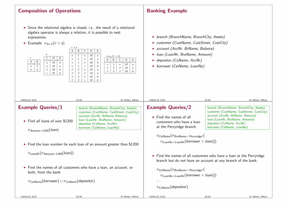
Composition of Operations
◮ Since the relational algebra is closed, i.e., the result of a relationalalgebra operator is always a relation, it is possible to nestexpressions.
◮ Example: σA=C (r × s)
r
A B
α 1
β 2
s
C D E
α 10 a
β 10 a
β 20 b
γ 10 b
r × s
A B C D E
α 1 α 10 a
α 1 β 10 a
α 1 β 20 b
α 1 γ 10 b
β 2 α 10 a
β 2 β 10 a
β 2 β 20 b
β 2 γ 10 b
σA=C (r × s)
A B C D E
α 1 α 10 a
β 2 β 10 a
β 2 β 20 b
Inf4Oec10, SL02 33/48 M. Bohlen, ifi@uzh
Banking Example
◮ branch (BranchName, BranchCity, Assets)
◮ customer (CustName, CustStreet, CustCity)
◮ account (AccNr, BrName, Balance)
◮ loan (LoanNr, BraName, Amount)
◮ depositor (CuName, AccNr)
◮ borrower (CstName, LoanNo)
Inf4Oec10, SL02 34/48 M. Bohlen, ifi@uzh
Example Queries/1 branch (BranchName, BranchCity, Assets)customer (CustName, CustStreet, CustCity)account (AccNr, BrName, Balance)loan (LoanNr, BraName, Amount)depositor (CuName, AccNr)borrower (CstName, LoanNo)
◮ Find all loans of over $1200
σAmount>1200(loan)
◮ Find the loan number for each loan of an amount greater than $1200
πLoanNr (σAmount>1200(loan))
◮ Find the names of all customers who have a loan, an account, orboth, from the bank
πCstName(borrower) ∪ πCuName(depositor)
Inf4Oec10, SL02 35/48 M. Bohlen, ifi@uzh
Example Queries/2 branch (BranchName, BranchCity, Assets)customer (CustName, CustStreet, CustCity)account (AccNr, BrName, Balance)loan (LoanNr, BraName, Amount)depositor (CuName, AccNr)borrower (CstName, LoanNo)
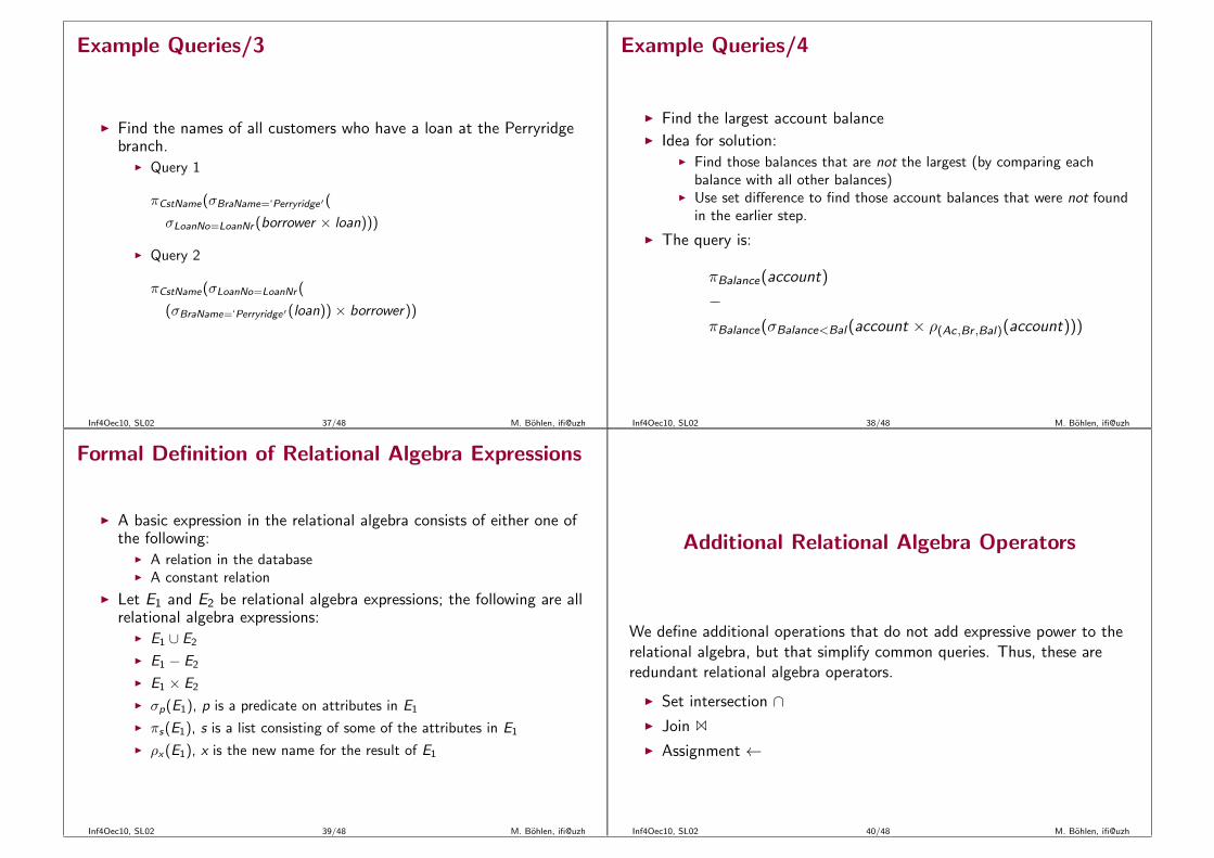
◮ Find the names of allcustomers who have a loanat the Perryridge branch.
πCstName(σBraName=‘Perryridge′(
σLoanNo=LoanNr (borrower × loan)))
◮ Find the names of all customers who have a loan at the Perryridgebranch but do not have an account at any branch of the bank.
πCstName(σBraName=‘Perryridge′(
σLoanNo=LoanNr (borrower × loan)))
−πCuName(depositor)
Inf4Oec10, SL02 36/48 M. Bohlen, ifi@uzh
Example Queries/3
◮ Find the names of all customers who have a loan at the Perryridgebranch.
◮ Query 1
πCstName(σBraName=‘Perryridge′(
σLoanNo=LoanNr (borrower × loan)))
◮ Query 2
πCstName(σLoanNo=LoanNr (
(σBraName=‘Perryridge′(loan))× borrower))
Inf4Oec10, SL02 37/48 M. Bohlen, ifi@uzh
Example Queries/4
◮ Find the largest account balance◮ Idea for solution:
◮ Find those balances that are not the largest (by comparing eachbalance with all other balances)
◮ Use set difference to find those account balances that were not foundin the earlier step.
◮ The query is:
πBalance(account)
−πBalance(σBalance<Bal(account × ρ(Ac,Br ,Bal)(account)))
Inf4Oec10, SL02 38/48 M. Bohlen, ifi@uzh
Formal Definition of Relational Algebra Expressions
◮ A basic expression in the relational algebra consists of either one ofthe following:
◮ A relation in the database◮ A constant relation
◮ Let E1 and E2 be relational algebra expressions; the following are allrelational algebra expressions:
◮ E1 ∪ E2
◮ E1 − E2
◮ E1 × E2
◮ σp(E1), p is a predicate on attributes in E1
◮ πs(E1), s is a list consisting of some of the attributes in E1
◮ ρx(E1), x is the new name for the result of E1
Inf4Oec10, SL02 39/48 M. Bohlen, ifi@uzh
Additional Relational Algebra Operators
We define additional operations that do not add expressive power to therelational algebra, but that simplify common queries. Thus, these areredundant relational algebra operators.
◮ Set intersection ∩◮ Join 1
◮ Assignment ←
Inf4Oec10, SL02 40/48 M. Bohlen, ifi@uzh
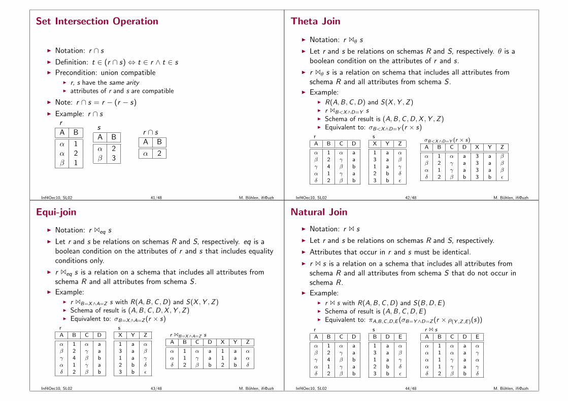
Set Intersection Operation
◮ Notation: r ∩ s
◮ Definition: t ∈ (r ∩ s)⇔ t ∈ r ∧ t ∈ s◮ Precondition: union compatible
◮ r, s have the same arity◮ attributes of r and s are compatible
◮ Note: r ∩ s = r − (r − s)
◮ Example: r ∩ sr
A B
α 1α 2β 1
s
A B
α 2β 3
r ∩ s
A B
α 2
Inf4Oec10, SL02 41/48 M. Bohlen, ifi@uzh
Theta Join
◮ Notation: r 1θ s
◮ Let r and s be relations on schemas R and S, respectively. θ is aboolean condition on the attributes of r and s.
◮ r 1θ s is a relation on schema that includes all attributes fromschema R and all attributes from schema S .
◮ Example:◮ R(A,B ,C ,D) and S(X ,Y ,Z )◮ r 1B<X∧D=Y s◮ Schema of result is (A,B ,C ,D,X ,Y ,Z )◮ Equivalent to: σB<X∧D=Y (r × s)
r
A B C D
α 1 α aβ 2 γ aγ 4 β bα 1 γ aδ 2 β b
s
X Y Z
1 a α
3 a β
1 a γ
2 b δ3 b ǫ
σB<X∧D=Y (r × s)
A B C D X Y Z
α 1 α a 3 a β
β 2 γ a 3 a β
α 1 γ a 3 a β
δ 2 β b 3 b ǫ
Inf4Oec10, SL02 42/48 M. Bohlen, ifi@uzh
Equi-join
◮ Notation: r 1eq s
◮ Let r and s be relations on schemas R and S, respectively. eq is aboolean condition on the attributes of r and s that includes equalityconditions only.
◮ r 1eq s is a relation on a schema that includes all attributes fromschema R and all attributes from schema S .
◮ Example:◮ r 1B=X∧A=Z s with R(A,B ,C ,D) and S(X ,Y ,Z )◮ Schema of result is (A,B ,C ,D,X ,Y ,Z )◮ Equivalent to: σB=X∧A=Z (r × s)
r
A B C D
α 1 α aβ 2 γ aγ 4 β bα 1 γ aδ 2 β b
s
X Y Z
1 a α
3 a β
1 a γ
2 b δ
3 b ǫ
r 1B=X∧A=Z s
A B C D X Y Z
α 1 α a 1 a α
α 1 γ a 1 a α
δ 2 β b 2 b δ
Inf4Oec10, SL02 43/48 M. Bohlen, ifi@uzh
Natural Join
◮ Notation: r 1 s
◮ Let r and s be relations on schemas R and S, respectively.
◮ Attributes that occur in r and s must be identical.
◮ r 1 s is a relation on a schema that includes all attributes fromschema R and all attributes from schema S that do not occur inschema R .
◮ Example:◮ r 1 s with R(A,B ,C ,D) and S(B ,D,E )◮ Schema of result is (A,B ,C ,D,E )◮ Equivalent to: πA,B,C ,D,E (σB=Y∧D=Z (r × ρ(Y ,Z ,E)(s))
r
A B C D
α 1 α aβ 2 γ aγ 4 β bα 1 γ aδ 2 β b
s
B D E
1 a α
3 a β
1 a γ
2 b δ
3 b ǫ
r 1 s
A B C D E
α 1 α a α
α 1 α a γ
α 1 γ a α
α 1 γ a γ
δ 2 β b δ
Inf4Oec10, SL02 44/48 M. Bohlen, ifi@uzh

Assignment Operation
◮ The assignment operation (←) provides a convenient way to expresscomplex queries by breaking them up into smaller pieces.
◮ Write query as a sequential program consisting of◮ a series of assignments◮ followed by an expression whose value is displayed as a result of the
query.
◮ Assignment must always be made to a temporary relation variable.
◮ Example: Write difference from slide 38 as
temp1← πBalance(account)temp2← πBalance(σBalance<Bal(account × ρ(Ac,Br ,Bal)(account)))result = temp1− temp2
◮ The result to the right of the ← is assigned to the relation variable onthe left of the ←.
Inf4Oec10, SL02 45/48 M. Bohlen, ifi@uzh
Bank Example Queries/1
◮ Find all customers who have an account and a loan.
πCustName(borrower) ∩ πCustName(depositor)
◮ Find the name of all customers who have a loan at the bank and theloan amount
Sol2 : πCstName,Amount(ρ(CstName,LoanNr)(borrower) 1 loan)
Sol1 : πCstName,Amount(borrower 1LoanNo=LoanNr loan)
Inf4Oec10, SL02 46/48 M. Bohlen, ifi@uzh
Bank Example Queries/2
◮ Find all customers who have an account from at least the“Downtown” and the “Uptown” branches.
◮ Solution:
πCuName(σBrName=‘Downtown′(depositor 1 account))
∩πCuName(σBrName=‘Uptown′(depositor 1 account))
Inf4Oec10, SL02 47/48 M. Bohlen, ifi@uzh
Summary
◮ The Relational Model◮ attribute, domain, tuple, relation, database, schema
◮ Basic Relational Algebra Operators◮ Selection σ◮ Projection π◮ Union ∪◮ Difference −◮ Cartesian product ×◮ Rename ρ
◮ Additional Relational Algebra Operators◮ Join (theta, natural) Join◮ Assignment ←
Inf4Oec10, SL02 48/48 M. Bohlen, ifi@uzh

Informatik fur Okonomen IIFall 2010
Database SystemsSQLSL03
◮ Data Definition Language
◮ Table Expressions, Query Specifications, Query Expressions
◮ Subqueries, Duplicates, Null Values
◮ Modification of the Database
Inf4Oec10, SL03 1/52 M. Bohlen, ifi@uzh
Checking...
1. Assume R(A) = {(1), (2), (3)}. Write a relational algebra expressionthat determines the larges value in R.
R
A
1
2
3
R1
A B
1 1
1 2
1 3
2 1
2 2
2 3
3 1
3 2
3 3
R2
A B
1 2
1 3
2 3
R3
A
3
R1← R × ρ(B)(R)
R2← σA<B(R1)
R3← R − πA(R2)
Inf4Oec10, SL03 2/52 M. Bohlen, ifi@uzh
Checking...
1. Identify and fix mistakes in the following relational algebraexpressions. Assume a relation with schema R(A,B).
σR.A>5(R)R.A is not an attribute name. Fix: σA>5(R)
σA,B(R)Selection requires predicate. Fix: πA,B(R)
R × RName clashes. Fix: ρT (R × ρS(C ,D)(R))
Inf4Oec10, SL03 3/52 M. Bohlen, ifi@uzh
History
◮ IBM Sequel language developed as part of System R project at theIBM San Jose Research Laboratory
◮ Renamed Structured Query Language (SQL)◮ ANSI and ISO standard SQL:
◮ SQL-86◮ SQL-89◮ SQL-92 (also called SQL2)
◮ entry level: roughly corresponds to SQL-89◮ intermediate level: half of the new features of SQL-92◮ full level
◮ SQL:2003 (also called SQL3)
◮ Commercial systems offer most, if not all, SQL-92 features, plusvarying feature sets from later standards and special proprietaryfeatures.
Inf4Oec10, SL03 4/52 M. Bohlen, ifi@uzh
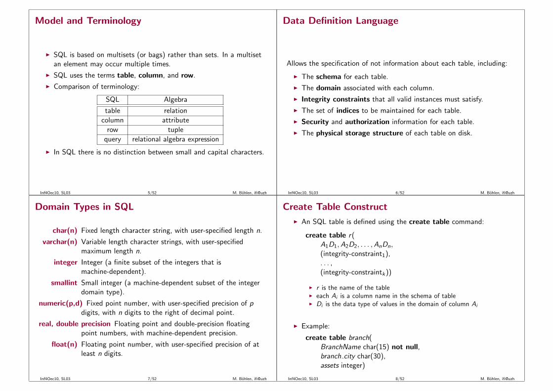
Model and Terminology
◮ SQL is based on multisets (or bags) rather than sets. In a multisetan element may occur multiple times.
◮ SQL uses the terms table, column, and row.
◮ Comparison of terminology:
SQL Algebra
table relation
column attribute
row tuple
query relational algebra expression
◮ In SQL there is no distinction between small and capital characters.
Inf4Oec10, SL03 5/52 M. Bohlen, ifi@uzh
Data Definition Language
Allows the specification of not information about each table, including:
◮ The schema for each table.
◮ The domain associated with each column.
◮ Integrity constraints that all valid instances must satisfy.
◮ The set of indices to be maintained for each table.
◮ Security and authorization information for each table.
◮ The physical storage structure of each table on disk.
Inf4Oec10, SL03 6/52 M. Bohlen, ifi@uzh
Domain Types in SQL
char(n) Fixed length character string, with user-specified length n.
varchar(n) Variable length character strings, with user-specifiedmaximum length n.
integer Integer (a finite subset of the integers that ismachine-dependent).
smallint Small integer (a machine-dependent subset of the integerdomain type).
numeric(p,d) Fixed point number, with user-specified precision of pdigits, with n digits to the right of decimal point.
real, double precision Floating point and double-precision floatingpoint numbers, with machine-dependent precision.
float(n) Floating point number, with user-specified precision of atleast n digits.
Inf4Oec10, SL03 7/52 M. Bohlen, ifi@uzh
Create Table Construct
◮ An SQL table is defined using the create table command:
create table r(A1D1,A2D2, . . . ,AnDn,(integrity-constraint1),. . . ,(integrity-constraintk))
◮ r is the name of the table◮ each Ai is a column name in the schema of table◮ Di is the data type of values in the domain of column Ai
◮ Example:
create table branch(BranchName char(15) not null,branch city char(30),assets integer)
Inf4Oec10, SL03 8/52 M. Bohlen, ifi@uzh

Integrity Constraints in Create Table
◮ not null
◮ primary key (A1, . . . ,An)
Example: Declare BranchName as the primary key for branch
create table branch(BranchName char(15),BranchCity char(30),Assets integer,primary key (BranchName))
In SQL a primary key declaration on a column automatically ensuresnot null.
Inf4Oec10, SL03 9/52 M. Bohlen, ifi@uzh
Drop and Alter Table Constructs
◮ The drop table command deletes all information about the droppedtable from the database.
◮ The alter table command is used to add columns to an existingtable:
alter table r add A D
where A is the name of the column to be added to table r and D isthe domain of A.
◮ All tuples in the table are assigned null as the value for the newcolumn.
◮ The alter table command can also be used to drop columns of atable:
alter table r drop A
where A is the name of an column of table r◮ Dropping of columns not supported by many databases
Inf4Oec10, SL03 10/52 M. Bohlen, ifi@uzh
Expressions and Predicates
◮ Powerful expressions and predicates make computer languages usefuland convenient.
◮ Database vendors compete on the set of expressions and predicatesthey offer (functionality as well as speed).
◮ In databases the efficient evaluation of predicates is a major concern.◮ Consider a table with 1 billion tuples and the following predicates:
◮ LastName = ’Miller’◮ LastName like ’%mann’◮ LastName like ’Ester%’
◮ That is one of the reasons why additions of (user defined) functionsand predicates to DBMS has been limited.
◮ We show some SQL expressions and predicates to give a rough ideaof common database functionality.
Inf4Oec10, SL03 11/52 M. Bohlen, ifi@uzh
Structure of SQL Queries/1
◮ SQL is based on relations and relational operations with certainmodifications and enhancements.
◮ It is used very heavily in the real world.
◮ Note that SQL is much more than simple select-from-where queriessuch as the following:
select *from Employeewhere LName = ’Bohr’
◮ Many people◮ Do not understand the concepts of SQL◮ Do not really understand how to work with a declarative language
and sets (this requires some practice and getting used to)◮ Underestimate SQL
Inf4Oec10, SL03 12/52 M. Bohlen, ifi@uzh
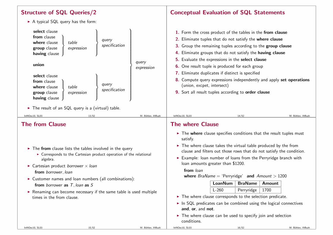
Structure of SQL Queries/2
◮ A typical SQL query has the form:
select clausefrom clausewhere clausegroup clausehaving clause
tableexpression
queryspecification
union
select clausefrom clausewhere clausegroup clausehaving clause
tableexpression
queryspecification
queryexpression
◮ The result of an SQL query is a (virtual) table.
Inf4Oec10, SL03 13/52 M. Bohlen, ifi@uzh
Conceptual Evaluation of SQL Statements
1. Form the cross product of the tables in the from clause
2. Eliminate tuples that do not satisfy the where clause
3. Group the remaining tuples according to the group clause
4. Eliminate groups that do not satisfy the having clause
5. Evaluate the expressions in the select clause
6. One result tuple is produced for each group
7. Eliminate duplicates if distinct is specified
8. Compute query expressions independently and apply set operations(union, excpet, intersect)
9. Sort all result tuples according to order clause
Inf4Oec10, SL03 14/52 M. Bohlen, ifi@uzh
The from Clause
◮ The from clause lists the tables involved in the query◮ Corresponds to the Cartesian product operation of the relational
algebra.
◮ Cartesian product borrower × loan
from borrower , loan
◮ Customer names and loan numbers (all combinations):
from borrower as T , loan as S
◮ Renaming can become necessary if the same table is used multipletimes in the from clause.
Inf4Oec10, SL03 15/52 M. Bohlen, ifi@uzh
The where Clause
◮ The where clause specifies conditions that the result tuples mustsatisfy.
◮ The where clause takes the virtual table produced by the fromclause and filters out those rows that do not satisfy the condition.
◮ Example: loan number of loans from the Perryridge branch withloan amounts greater than $1200.
from loanwhere BraName = ‘Perryridge’ and Amount > 1200
LoanNum BraName Amount
L-260 Perryridge 1700
◮ The where clause corresponds to the selection predicate.
◮ In SQL predicates can be combined using the logical connectivesand, or, and not.
◮ The where clause can be used to specify join and selectionconditions.
Inf4Oec10, SL03 16/52 M. Bohlen, ifi@uzh

The group Clause◮ The group clause takes the table produced by the where clause and
returns a grouped table.◮ The group clause groups multiple tuples together. Conceptually,
grouping yields multiple tables.◮ Example: Accounts grouped by branch.
from accountgroup by BrName
account
AccNr BrName Balance
A-101 Downtown 500
A-215 Perryridge 700
A-102 Perryridge 400
A-305 Perryridge 350
A-222 Perryridge 700
A-201 Brighton 900
A-217 Brighton 750
Inf4Oec10, SL03 17/52 M. Bohlen, ifi@uzh
The having Clause/1
◮ The having clause takes a grouped table as input and returns agrouped table.
◮ The having condition is applied to each group.
◮ Only groups that fulfill the condition are returned.
◮ The having clause never returns individual tuples of a group.
◮ The having condition may include grouping columns or aggregatedcolumns.
Inf4Oec10, SL03 18/52 M. Bohlen, ifi@uzh
The having Clause/2
◮ Consider branches with more than one account only:
from accountgroup by BrNamehaving count(AccNr) > 1
◮ This having clause returns all groups with more than one tuple:
account
AccNr BrName Balance
A-215 Perryridge 700
A-102 Perryridge 400
A-305 Perryridge 350
A-222 Perryridge 700
A-201 Brighton 900
A-217 Brighton 750
Inf4Oec10, SL03 19/52 M. Bohlen, ifi@uzh
The select Clause/1
◮ The select clause lists the columns that shall be in the result of aquery.
◮ corresponds to the projection operation of the relational algebra
◮ Example: find the names of all branches in the loan table:
select BraNamefrom loan
◮ In the relational algebra, the query would be:
πBraName(loan)
Inf4Oec10, SL03 20/52 M. Bohlen, ifi@uzh
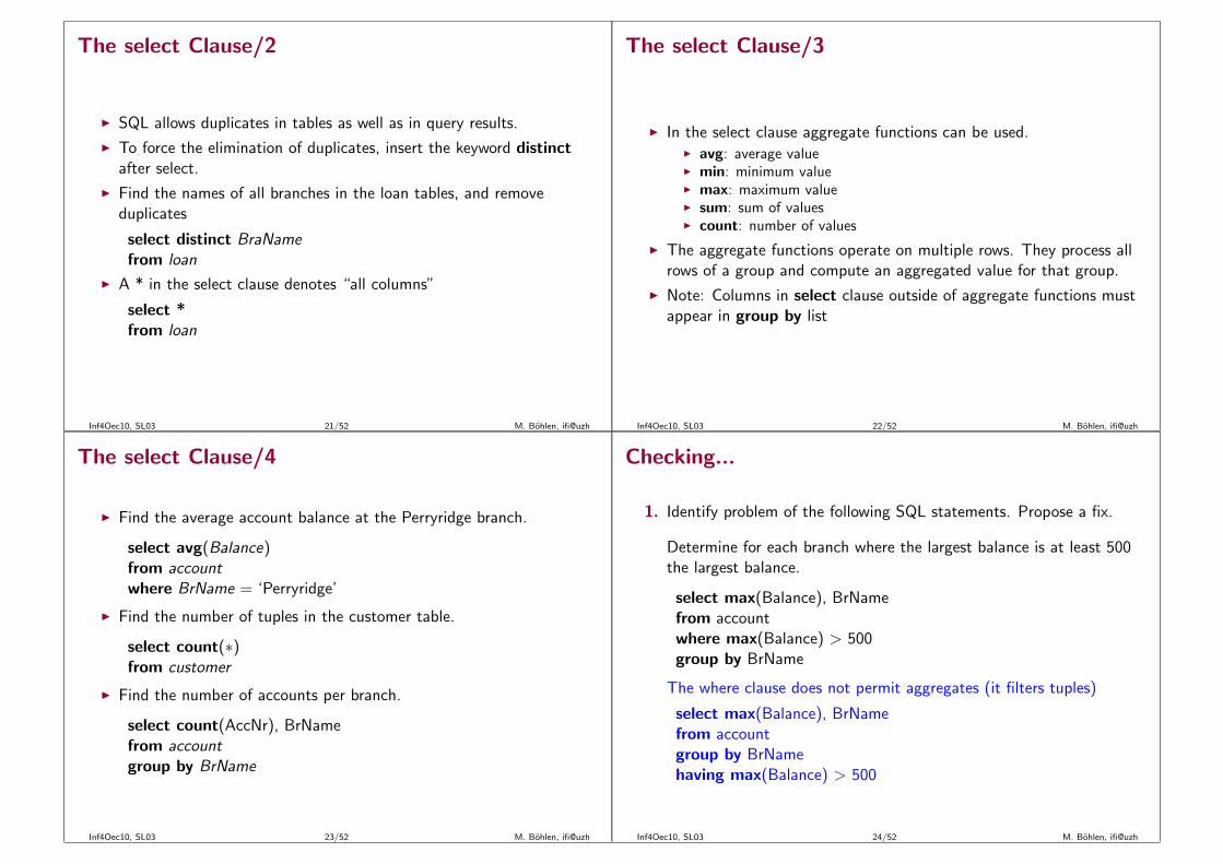
The select Clause/2
◮ SQL allows duplicates in tables as well as in query results.
◮ To force the elimination of duplicates, insert the keyword distinctafter select.
◮ Find the names of all branches in the loan tables, and removeduplicates
select distinct BraNamefrom loan
◮ A * in the select clause denotes “all columns”
select *from loan
Inf4Oec10, SL03 21/52 M. Bohlen, ifi@uzh
The select Clause/3
◮ In the select clause aggregate functions can be used.◮ avg: average value◮ min: minimum value◮ max: maximum value◮ sum: sum of values◮ count: number of values
◮ The aggregate functions operate on multiple rows. They process allrows of a group and compute an aggregated value for that group.
◮ Note: Columns in select clause outside of aggregate functions mustappear in group by list
Inf4Oec10, SL03 22/52 M. Bohlen, ifi@uzh
The select Clause/4
◮ Find the average account balance at the Perryridge branch.
select avg(Balance)from accountwhere BrName = ‘Perryridge’
◮ Find the number of tuples in the customer table.
select count(∗)from customer
◮ Find the number of accounts per branch.
select count(AccNr), BrNamefrom accountgroup by BrName
Inf4Oec10, SL03 23/52 M. Bohlen, ifi@uzh
Checking...
1. Identify problem of the following SQL statements. Propose a fix.
Determine for each branch where the largest balance is at least 500the largest balance.
select max(Balance), BrNamefrom accountwhere max(Balance) > 500group by BrName
The where clause does not permit aggregates (it filters tuples)
select max(Balance), BrNamefrom accountgroup by BrNamehaving max(Balance) > 500
Inf4Oec10, SL03 24/52 M. Bohlen, ifi@uzh

Checking...account
AccNr BrName Balance
A-101 Downtown 500
A-215 Perryridge 700
A-102 Perryridge 400
A-305 Perryridge 350
A-222 Perryridge 700
A-201 Brighton 900
A-217 Brighton 750
2. Identify problem of the followingSQL statements.
Determine for each branch theaccount with the largest balance.
select max(Balance), AccNr, BrNamefrom accountgroup by BrName
In the select clause only aggregates or grouped columns are allowed.The reason for this constraint is that exactly one tuple per groupshall be computed.
The above query must be solved with a subquery.
Inf4Oec10, SL03 25/52 M. Bohlen, ifi@uzh
SQL so far
◮ SQL versus relational algebra:
SQL Algebra
table relation
column attribute
row tuple
query relational algebra expression
◮ A query specification in SQL has the following form:
select clausefrom clausewhere clausegroup clausehaving clause
tableexpression
queryspecification
Inf4Oec10, SL03 26/52 M. Bohlen, ifi@uzh
Illustration of Evaluation of SQL Statements/1
1. FROM: form the cross product of the tables in the from clause
FROM...
2. WHERE: eliminate tuples that do not satisfy the where clause
...WHERE
3. GROUP BY: group tuples according to the group clause
GROUP BY
Inf4Oec10, SL03 27/52 M. Bohlen, ifi@uzh
Illustration of Evaluation of SQL Statements/2
4. HAVING: eliminate groups that do not satisfy the having clause
HAVING
5. SELECT: evaluate the expressions in the select clause and produceone result tuple for each group
SELECT
Inf4Oec10, SL03 28/52 M. Bohlen, ifi@uzh

Query Expressions/1
◮ The set operations union, intersect, and except operate on tablesand correspond to the relational algebra operations ∪, ∩ , −
◮ Each of the above operations automatically eliminates duplicates; toretain all duplicates use the corresponding multiset versions unionall, intersect all, and except all.
Suppose a tuple occurs m times in r and n times in s, then, itoccurs:
◮ m + n times in r union all s◮ min(m, n) times in r intersect all s◮ max(0,m − n) times in r except all s
Inf4Oec10, SL03 29/52 M. Bohlen, ifi@uzh
Query Expressions/2
◮ Find all customers who have a loan, an account, or both:
(select CuName from depositor)union(select CstName from borrower)
◮ Find all customers who have both a loan and an account:
(select CuName from depositor)intersect(select CstName from borrower)
◮ Find all customers who have an account but no loan:
(select CuName from depositor)except(select CstName from borrower)
Inf4Oec10, SL03 30/52 M. Bohlen, ifi@uzh
Subqueries/1
◮ SQL provides a mechanism for the nesting of subqueries.
◮ A subquery is a query expression that is nested within anotherquery expression.
◮ A common use of subqueries is to perform tests for set membership,set comparisons, and set cardinality.
Inf4Oec10, SL03 31/52 M. Bohlen, ifi@uzh
Subqueries/2
◮ Find all customers who have both an account and a loan at thebank.
select distinct CstNamefrom borrowerwhere CstName in (select CuName
from depositor)
◮ Find all customers who have a loan at the bank but do not have anaccount at the bank
select distinct CstNamefrom borrowerwhere CstName not in (select CuName
from depositor)
Inf4Oec10, SL03 32/52 M. Bohlen, ifi@uzh

Subqueries/3
◮ Find all customers who have both an account and a loan at thePerryridge branch
select distinct CstNamefrom borrower , loanwhere borrower .LoanNo = loan.LoanNrand BraName = ‘Perryridge’and (BraName,CstName) in (
select BrName,CuNamefrom depositor , accountwhere depositor .AccNr = account.AccNr)
Inf4Oec10, SL03 33/52 M. Bohlen, ifi@uzh
Subqueries/4Comparing sets:
◮ Find all branches that have greater assets than some branch locatedin Brooklyn.
select distinct T .BranchNamefrom branch as T , branch as Swhere T .Assets > S .Assets andS .BranchCity = ‘Brooklyn’
◮ Same query using > some clause
select BranchNamefrom branchwhere Assets > some
(select Assetsfrom branchwhere BranchCity = ‘Brooklyn’)
Inf4Oec10, SL03 34/52 M. Bohlen, ifi@uzh
Subqueries/5◮ F <comp> some r ⇔ ∃t ∈ r such that (F <comp> t)
Where <comp> can be: <,≤ , >,=, 6=
(5 < some0
5
6
) = true
(read: 5 < some tuple in the table)
(5 < some0
5) = false
(5 = some0
5) = true
(5 6= some0
5) = true (since 0 6= 5)
(= some) ≡ inHowever, ( 6= some) 6≡ not in
Inf4Oec10, SL03 35/52 M. Bohlen, ifi@uzh
Subqueries/6
◮ Find the names of all branches that have greater assets than allbranches located in Brooklyn.
select BranchNamefrom branchwhere assets > all
(select assetsfrom branchwhere BranchCity = ‘Brooklyn’)
Inf4Oec10, SL03 36/52 M. Bohlen, ifi@uzh

Subqueries/7
◮ F <comp> all r ⇔ ∃t ∈ r (F <comp> t)
(5 < all0
5
6
) = false
(5 < all6
10) = true
(5 = all4
5) = false
(5 6= all4
6) = true (since 5 6= 4 and 5 6= 6)
( 6= all) ≡ not inHowever, (= all) 6≡ in
Inf4Oec10, SL03 37/52 M. Bohlen, ifi@uzh
Subqueries/8
◮ The exists construct returns the value true if the argumentsubquery is nonempty.
◮ exists r ⇔ r 6= ∅◮ not exists r ⇔ r = ∅◮ The exists (and not exists) subqueries are used frequently in SQL.
◮ Avoid in, all, any, some and use exists instead.
Inf4Oec10, SL03 38/52 M. Bohlen, ifi@uzh
Subqueries/9
◮ Find all customers who have an account at all branches located inBrooklyn.
select distinct S .CuNamefrom depositor as Swhere not exists (
(select BranchNamefrom branchwhere BranchCity = ‘Brooklyn’)except(select R .BrNamefrom depositor as T , account as Rwhere T .AccNr = R .AccNr and
S .CuName = T .CuName))
◮ Note that X − Y = ∅ ⇔ X ⊆ Y
◮ Note: Cannot write this query using = all and its variants
Inf4Oec10, SL03 39/52 M. Bohlen, ifi@uzh
Derived Tables
◮ SQL allows a subquery expression to be used in the from clause.
◮ That is important for orthogonality of a language.
◮ A derived table is defined by a query expression.
◮ Find the average account balance of those branches where theaverage account balance is greater than $1200.
select BranchName,AvgBalancefrom (select BrName, avg(Balance)
from accountgroup by account)as BranchAvg(BranchName,AvgBalance)
where AvgBalance > 1200
Inf4Oec10, SL03 40/52 M. Bohlen, ifi@uzh

Duplicates/1
◮ In tables with duplicates, SQL can define how many copies of tuplesappear in the result.
◮ Multiset versions of some of the relational algebra operators - givenmultiset relations r1 and r2:
1. σbθ(r1): If there are c1 copies of tuple t1 in r1, and t1 satisfies
selections σθ, then there are c1 copies of t1 in σbθ(r1).
2. πbA(r1): For each copy of tuple t1 in r1, there is a copy of tuple πA(t1)
in πbA(r1) where πA(t1) denotes the projection of the single tuple t1.
3. r1 ×b r2: If there are c1 copies of tuple t1 in r1 and r2 copies of tuplet2 in r2, there are c1 × c2 copies of the tuple t1, t2 in r1 ×b r2
Inf4Oec10, SL03 41/52 M. Bohlen, ifi@uzh
Duplicates/2
◮ Example: Suppose multisets r1(A,B) and r2(C ) are as follows:
r1 = {(1, a) (2, a)} r2 = {(2), (3), (3)}
◮ Then πbB(r1) would be {(a), (a)}, while πb
B(r1)× r2 would be
{(a, 2), (a, 2), (a, 3), (a, 3), (a, 3), (a, 3)}
◮ SQL duplicate semantics:
select A1,A2, . . . ,An
from r1, r2, . . . , rmwhere P
is equivalent to the multiset expression:
πbA1,A2,...,An(σ
bP(r1 ×b r2 ×b . . . ×b rm))
Inf4Oec10, SL03 42/52 M. Bohlen, ifi@uzh
Null Values/1
◮ It is possible for tuples to have a null value, denoted by null, forsome of their columns
◮ null signifies an unknown value or that a value does not exist.
◮ The predicate is null can be used to check for null values.
◮ Example: Find all loan number which appear in the loan relation withnull values for Amount.
select LoanNrfrom loanwhere Amount is null
◮ The result of any arithmetic expression involving null is null
◮ Example: 5 + null returns null
◮ However, aggregate functions simply ignore nulls◮ More on next slide
Inf4Oec10, SL03 43/52 M. Bohlen, ifi@uzh
Null Values/2
◮ Any comparison with null returns unknown◮ Example: 5 < null or null <> null or null = null
◮ Three-valued logic using the truth value unknown:◮ OR
(unknown or true) = true,(unknown or false) = unknown(unknown or unknown) = unknown
◮ AND(true and unknown) = unknown,(false and unknown) = false(unknown and unknown) = unknown
◮ NOT
(not unknown) = unknown◮ “P is unknown” evaluates to true if predicate P evaluates to
unknown
◮ Result of where clause predicate is treated as false if it evaluates tounknown
Inf4Oec10, SL03 44/52 M. Bohlen, ifi@uzh
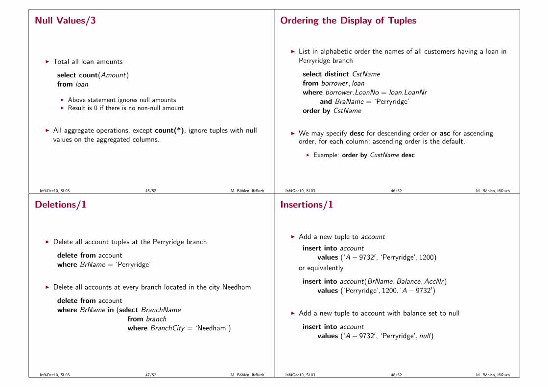
Null Values/3
◮ Total all loan amounts
select count(Amount)from loan
◮ Above statement ignores null amounts◮ Result is 0 if there is no non-null amount
◮ All aggregate operations, except count(*), ignore tuples with nullvalues on the aggregated columns.
Inf4Oec10, SL03 45/52 M. Bohlen, ifi@uzh
Ordering the Display of Tuples
◮ List in alphabetic order the names of all customers having a loan inPerryridge branch
select distinct CstNamefrom borrower , loanwhere borrower .LoanNo = loan.LoanNr
and BraName = ‘Perryridge’order by CstName
◮ We may specify desc for descending order or asc for ascendingorder, for each column; ascending order is the default.
◮ Example: order by CustName desc
Inf4Oec10, SL03 46/52 M. Bohlen, ifi@uzh
Deletions/1
◮ Delete all account tuples at the Perryridge branch
delete from accountwhere BrName = ‘Perryridge’
◮ Delete all accounts at every branch located in the city Needham
delete from accountwhere BrName in (select BranchName
from branchwhere BranchCity = ‘Needham’)
Inf4Oec10, SL03 47/52 M. Bohlen, ifi@uzh
Insertions/1
◮ Add a new tuple to account
insert into accountvalues (‘A− 9732′, ‘Perryridge’, 1200)
or equivalently
insert into account(BrName,Balance,AccNr)values (‘Perryridge’, 1200, ‘A− 9732′)
◮ Add a new tuple to account with balance set to null
insert into accountvalues (‘A− 9732′, ‘Perryridge’, null)
Inf4Oec10, SL03 48/52 M. Bohlen, ifi@uzh
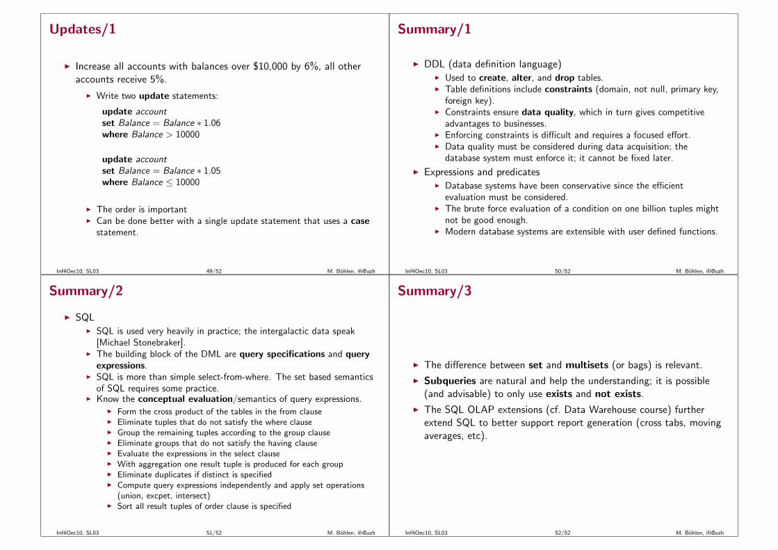
Updates/1
◮ Increase all accounts with balances over $10,000 by 6%, all otheraccounts receive 5%.
◮ Write two update statements:
update accountset Balance = Balance ∗ 1.06where Balance > 10000
update accountset Balance = Balance ∗ 1.05where Balance ≤ 10000
◮ The order is important◮ Can be done better with a single update statement that uses a case
statement.
Inf4Oec10, SL03 49/52 M. Bohlen, ifi@uzh
Summary/1
◮ DDL (data definition language)◮ Used to create, alter, and drop tables.◮ Table definitions include constraints (domain, not null, primary key,
foreign key).◮ Constraints ensure data quality, which in turn gives competitive
advantages to businesses.◮ Enforcing constraints is difficult and requires a focused effort.◮ Data quality must be considered during data acquisition; the
database system must enforce it; it cannot be fixed later.
◮ Expressions and predicates◮ Database systems have been conservative since the efficient
evaluation must be considered.◮ The brute force evaluation of a condition on one billion tuples might
not be good enough.◮ Modern database systems are extensible with user defined functions.
Inf4Oec10, SL03 50/52 M. Bohlen, ifi@uzh
Summary/2
◮ SQL◮ SQL is used very heavily in practice; the intergalactic data speak
[Michael Stonebraker].◮ The building block of the DML are query specifications and query
expressions.◮ SQL is more than simple select-from-where. The set based semantics
of SQL requires some practice.◮ Know the conceptual evaluation/semantics of query expressions.
◮ Form the cross product of the tables in the from clause◮ Eliminate tuples that do not satisfy the where clause◮ Group the remaining tuples according to the group clause◮ Eliminate groups that do not satisfy the having clause◮ Evaluate the expressions in the select clause◮ With aggregation one result tuple is produced for each group◮ Eliminate duplicates if distinct is specified◮ Compute query expressions independently and apply set operations
(union, excpet, intersect)◮ Sort all result tuples of order clause is specified
Inf4Oec10, SL03 51/52 M. Bohlen, ifi@uzh
Summary/3
◮ The difference between set and multisets (or bags) is relevant.
◮ Subqueries are natural and help the understanding; it is possible(and advisable) to only use exists and not exists.
◮ The SQL OLAP extensions (cf. Data Warehouse course) furtherextend SQL to better support report generation (cross tabs, movingaverages, etc).
Inf4Oec10, SL03 52/52 M. Bohlen, ifi@uzh
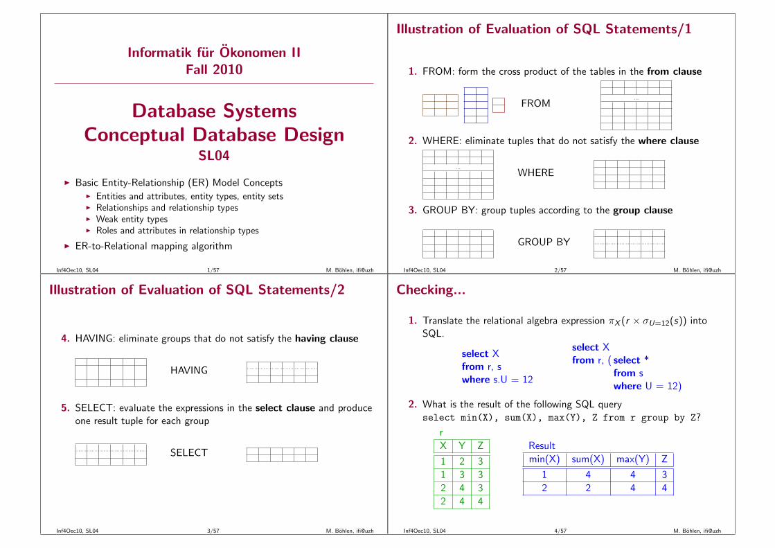
Informatik fur Okonomen IIFall 2010
Database SystemsConceptual Database Design
SL04
◮ Basic Entity-Relationship (ER) Model Concepts◮ Entities and attributes, entity types, entity sets◮ Relationships and relationship types◮ Weak entity types◮ Roles and attributes in relationship types
◮ ER-to-Relational mapping algorithm
Inf4Oec10, SL04 1/57 M. Bohlen, ifi@uzh
Illustration of Evaluation of SQL Statements/1
1. FROM: form the cross product of the tables in the from clause
FROM...
2. WHERE: eliminate tuples that do not satisfy the where clause
...WHERE
3. GROUP BY: group tuples according to the group clause
GROUP BY
Inf4Oec10, SL04 2/57 M. Bohlen, ifi@uzh
Illustration of Evaluation of SQL Statements/2
4. HAVING: eliminate groups that do not satisfy the having clause
HAVING
5. SELECT: evaluate the expressions in the select clause and produceone result tuple for each group
SELECT
Inf4Oec10, SL04 3/57 M. Bohlen, ifi@uzh
Checking...
r
X Y Z
1 2 3
1 3 3
2 4 3
2 4 4
Result
min(X) sum(X) max(Y) Z
1 4 4 3
2 2 4 4
1. Translate the relational algebra expression πX (r × σU=12(s)) intoSQL.
select Xfrom r, swhere s.U = 12
select Xfrom r, ( select *
from swhere U = 12)
2. What is the result of the following SQL queryselect min(X), sum(X), max(Y), Z from r group by Z?
Inf4Oec10, SL04 4/57 M. Bohlen, ifi@uzh
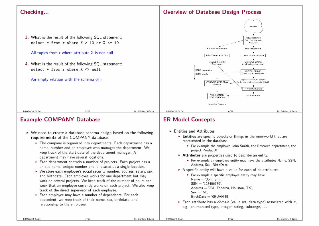
Checking...
3. What is the result of the following SQL statement:select * from r where X > 10 or X <= 10
All tuples from r where attribute X is not null
4. What is the result of the following SQL statement:select * from r where X <> null
An empty relation with the schema of r
Inf4Oec10, SL04 5/57 M. Bohlen, ifi@uzh
Overview of Database Design Process
Inf4Oec10, SL04 6/57 M. Bohlen, ifi@uzh
Example COMPANY Database
◮ We need to create a database schema design based on the followingrequirements of the COMPANY database:
◮ The company is organized into departments. Each department has aname, number and an employee who manages the department. Wekeep track of the start date of the department manager. Adepartment may have several locations.
◮ Each department controls a number of projects. Each project has aunique name, unique number and is located at a single location.
◮ We store each employee’s social security number, address, salary, sex,and birthdate. Each employee works for one department but maywork on several projects. We keep track of the number of hours perweek that an employee currently works on each project. We also keeptrack of the direct supervisor of each employee.
◮ Each employee may have a number of dependents. For eachdependent, we keep track of their name, sex, birthdate, andrelationship to the employee.
Inf4Oec10, SL04 7/57 M. Bohlen, ifi@uzh
ER Model Concepts
◮ Entities and Attributes◮ Entities are specific objects or things in the mini-world that are
represented in the database.◮ For example the employee John Smith, the Research department, the
project ProductX
◮ Attributes are properties used to describe an entity.◮ For example an employee entity may have the attributes Name, SSN,
Address, Sex, BirthDate
◮ A specific entity will have a value for each of its attributes.◮ For example a specific employee entity may have
Name = ’John Smith’,SSN = ’123456789’,Address = ’731, Fondren, Houston, TX’,Sex = ’M’,BirthDate = ’09-JAN-55‘
◮ Each attribute has a domain (value set, data type) associated with it,e.g., enumerated type, integer, string, subrange, . . .
Inf4Oec10, SL04 8/57 M. Bohlen, ifi@uzh

Types of Attributes/1
◮ Simple attribute◮ Each entity has a single atomic value for the attribute. For example,
SSN or Sex.
◮ Composite attribute◮ The attribute may be composed of several components. For example:
◮ Address(Apt#, House#, Street, City, State, ZipCode, Country), or◮ Name(FirstName, MiddleName, LastName).
◮ Multi-valued attribute◮ An entity may have multiple values for that attribute. For example,
Color of a CAR or PreviousDegrees of a STUDENT.◮ Denoted as {Color} or {PreviousDegrees}.
◮ Derived attribute◮ Attributes can be derived (computed) rather than stored. Attribute
Number of employees is a derived attribute of DEPARTMENT.
Inf4Oec10, SL04 9/57 M. Bohlen, ifi@uzh
Types of Attributes/2
◮ Composite and multi-valued attributes may be nested arbitrarily toany number of levels.
◮ For example, PreviousDegrees of a student is a compositemulti-valued attribute denoted by {PreviousDegrees (College, Year,Degree, Field)}
◮ Multiple PreviousDegrees values can exist◮ Each has four subcomponent attributes:
◮ College, Year, Degree, Field
◮ A hierarchy of composite attributes:Address
Street address City State Zip
Number Street Apartment number
Inf4Oec10, SL04 10/57 M. Bohlen, ifi@uzh
Entity Types and Key Attributes
◮ Entities with the same basic attributes are grouped or typed into anentity type.
◮ For example, the entity type EMPLOYEE and PROJECT.
◮ An attribute of an entity type for which each entity must have aunique value is called a key attribute of the entity type.
◮ For example, SSN of EMPLOYEE.
◮ A key attribute may be composite.◮ VehicleTagNumber is a key of the CAR entity type with components
(Number, State).
◮ An entity type may have more than one key.◮ The CAR entity type may have two keys:
◮ VehicleIdentificationNumber (popularly called VIN)◮ VehicleTagNumber (Number, State), aka license plate number.
◮ Each key is underlined.
Inf4Oec10, SL04 11/57 M. Bohlen, ifi@uzh
Displaying an Entity type
◮ In ER diagrams, an entity type is displayed in a rectangular box◮ Attributes are displayed in ovals
◮ Each attribute is connected to its entity type◮ Components of a composite attribute are connected to the oval
representing the composite attribute◮ Each key attribute is underlined◮ Multivalued attributes are displayed in double ovals◮ Derived attributes are displayed in dashed ovals
◮ Entity type CAR with attributes Registration(Number, State),Vehicle id, Make, Model, Year, {Color}
Inf4Oec10, SL04 12/57 M. Bohlen, ifi@uzh

Entity Set
◮ The collection of all entities of a particular entity type in thedatabase is called the entity set.
◮ The same name (e.g., CAR) is used to refer to both the entity typeand the entity set.
◮ The entity set is the current state of the entities of that type thatare stored in the database.
◮ Entity set CAR:
Inf4Oec10, SL04 13/57 M. Bohlen, ifi@uzh
Entity Types for the COMPANY Database/1
◮ Based on the requirements, we can identify four initial entity typesin the COMPANY database:
◮ DEPARTMENT◮ PROJECT◮ EMPLOYEE◮ DEPENDENT
◮ The initial attributes are derived from the requirements description◮ Guidelines for determining entity types and attributes:
◮ The nouns in a descriptions translate to entity types◮ Nouns that describe nouns of entity types translate to attributes.
Inf4Oec10, SL04 14/57 M. Bohlen, ifi@uzh
Entity Types for the COMPANY Database/2
Inf4Oec10, SL04 15/57 M. Bohlen, ifi@uzh
Relationships and Relationship Types/1
◮ The initial design is typically not complete.
◮ The schema design process is an iterative refinement process. Theinitial design is created and iteratively refined.
◮ Some aspects in the requirements will be represented asrelationships.
◮ ER model has three main concepts:◮ Entities (and their entity types and entity sets)◮ Attributes (simple, composite, multivalued)◮ Relationships (and their relationship types and relationship sets)
Inf4Oec10, SL04 16/57 M. Bohlen, ifi@uzh

Relationships and Relationship Types/2
◮ A relationship relates two or more distinct entities with a specificmeaning.
◮ For example, EMPLOYEE John Smith works on PROJECTProductX, or EMPLOYEE Franklin Wong manages the ResearchDEPARTMENT.
◮ Relationships of the same type are grouped or typed into arelationship type.
◮ For example, the WORKS ON relationship type in whichEMPLOYEEs and PROJECTs participate, or the MANAGESrelationship type in which EMPLOYEEs and DEPARTMENTsparticipate.
◮ The degree of a relationship type is the number of participatingentity types.
◮ Both MANAGES and WORKS ON are binary relationships.
Inf4Oec10, SL04 17/57 M. Bohlen, ifi@uzh
Relationships and Relationship Types/3
◮ Relationship type:◮ Schema description of a relationship◮ Identifies the relationship name and the participating entity types◮ Identifies relationship constraints
◮ Relationship set:◮ The current set of relationship instances represented in the database◮ The current state of a relationship type
◮ Each instance in the set relates individual participating entities – onefrom each participating entity type
Inf4Oec10, SL04 18/57 M. Bohlen, ifi@uzh
WORKS FOR relationship
◮ entity: e1◮ relationship: r1 = WORKS FOR(e1,d1)
◮ entity set: EMPLOYEE
◮ relationship set: WORKS FOR
Inf4Oec10, SL04 19/57 M. Bohlen, ifi@uzh
Relationships for the COMPANY database/1
◮ By examining the requirements, six relationship types are identified
◮ All are binary relationships (degree 2)◮ Listed below with their participating entity types:
◮ WORKS FOR (between EMPLOYEE and DEPARTMENT)◮ MANAGES (also between EMPLOYEE and DEPARTMENT)◮ CONTROLS (between DEPARTMENT and PROJECT)◮ WORKS ON (between EMPLOYEE and PROJECT)◮ SUPERVISION (between EMPLOYEE (as subordinate) and
EMPLOYEE (as supervisor))◮ DEPENDENTS OF (between EMPLOYEE and DEPENDENT)
◮ In ER diagrams, we represent the relationship type as follows:◮ Diamond-shaped box is used to display a relationship type◮ Connected to the participating entity types via straight lines
Inf4Oec10, SL04 20/57 M. Bohlen, ifi@uzh
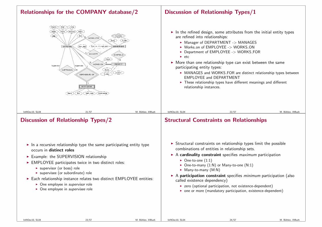
Relationships for the COMPANY database/2
Inf4Oec10, SL04 21/57 M. Bohlen, ifi@uzh
Discussion of Relationship Types/1
◮ In the refined design, some attributes from the initial entity typesare refined into relationships:
◮ Manager of DEPARTMENT -> MANAGES◮ Works on of EMPLOYEE -> WORKS ON◮ Department of EMPLOYEE -> WORKS FOR◮ etc
◮ More than one relationship type can exist between the sameparticipating entity types:
◮ MANAGES and WORKS FOR are distinct relationship types betweenEMPLOYEE and DEPARTMENT
◮ These relationship types have different meanings and differentrelationship instances.
Inf4Oec10, SL04 22/57 M. Bohlen, ifi@uzh
Discussion of Relationship Types/2
◮ In a recursive relationship type the same participating entity typeoccurs in distinct roles
◮ Example: the SUPERVISION relationship◮ EMPLOYEE participates twice in two distinct roles:
◮ supervisor (or boss) role◮ supervisee (or subordinate) role
◮ Each relationship instance relates two distinct EMPLOYEE entities:◮ One employee in supervisor role◮ One employee in supervisee role
Inf4Oec10, SL04 23/57 M. Bohlen, ifi@uzh
Structural Constraints on Relationships
◮ Structural constraints on relationship types limit the possiblecombinations of entities in relationship sets.
◮ A cardinality constraint specifies maximum participation◮ One-to-one (1:1)◮ One-to-many (1:N) or Many-to-one (N:1)◮ Many-to-many (M:N)
◮ A participation constraint specifies minimum participation (alsocalled existence dependency)
◮ zero (optional participation, not existence-dependent)◮ one or more (mandatory participation, existence-dependent)
Inf4Oec10, SL04 24/57 M. Bohlen, ifi@uzh
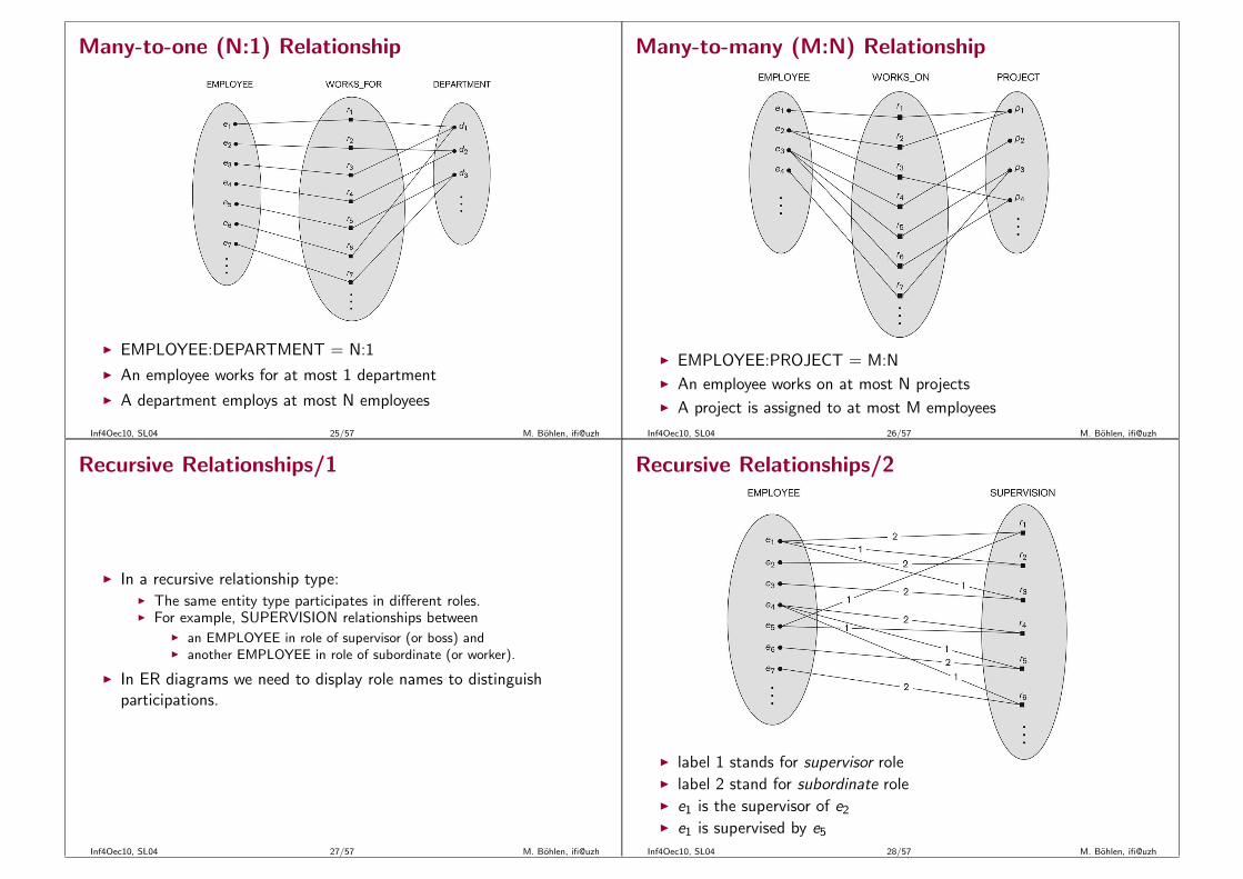
Many-to-one (N:1) Relationship
◮ EMPLOYEE:DEPARTMENT = N:1
◮ An employee works for at most 1 department
◮ A department employs at most N employees
Inf4Oec10, SL04 25/57 M. Bohlen, ifi@uzh
Many-to-many (M:N) Relationship
◮ EMPLOYEE:PROJECT = M:N
◮ An employee works on at most N projects
◮ A project is assigned to at most M employees
Inf4Oec10, SL04 26/57 M. Bohlen, ifi@uzh
Recursive Relationships/1
◮ In a recursive relationship type:◮ The same entity type participates in different roles.◮ For example, SUPERVISION relationships between
◮ an EMPLOYEE in role of supervisor (or boss) and◮ another EMPLOYEE in role of subordinate (or worker).
◮ In ER diagrams we need to display role names to distinguishparticipations.
Inf4Oec10, SL04 27/57 M. Bohlen, ifi@uzh
Recursive Relationships/2
◮ label 1 stands for supervisor role◮ label 2 stand for subordinate role◮ e1 is the supervisor of e2◮ e1 is supervised by e5
Inf4Oec10, SL04 28/57 M. Bohlen, ifi@uzh
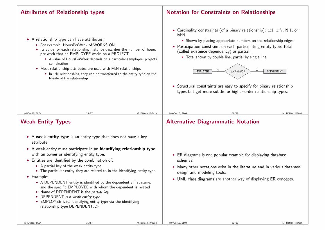
Attributes of Relationship types
◮ A relationship type can have attributes:◮ For example, HoursPerWeek of WORKS ON◮ Its value for each relationship instance describes the number of hours
per week that an EMPLOYEE works on a PROJECT.◮ A value of HoursPerWeek depends on a particular (employee, project)
combination
◮ Most relationship attributes are used with M:N relationships◮ In 1:N relationships, they can be transferred to the entity type on the
N-side of the relationship
Inf4Oec10, SL04 29/57 M. Bohlen, ifi@uzh
Notation for Constraints on Relationships
◮ Cardinality constraints (of a binary relationship): 1:1, 1:N, N:1, orM:N
◮ Shown by placing appropriate numbers on the relationship edges.
◮ Participation constraint on each participating entity type: total(called existence dependency) or partial.
◮ Total shown by double line, partial by single line.
◮ Structural constraints are easy to specify for binary relationshiptypes but get more subtle for higher order relationship types.
Inf4Oec10, SL04 30/57 M. Bohlen, ifi@uzh
Weak Entity Types
◮ A weak entity type is an entity type that does not have a keyattribute.
◮ A weak entity must participate in an identifying relationship typewith an owner or identifying entity type.
◮ Entities are identified by the combination of:◮ A partial key of the weak entity type◮ The particular entity they are related to in the identifying entity type
◮ Example:◮ A DEPENDENT entity is identified by the dependent’s first name,
and the specific EMPLOYEE with whom the dependent is related◮ Name of DEPENDENT is the partial key◮ DEPENDENT is a weak entity type◮ EMPLOYEE is its identifying entity type via the identifying
relationship type DEPENDENT OF
Inf4Oec10, SL04 31/57 M. Bohlen, ifi@uzh
Alternative Diagrammatic Notation
◮ ER diagrams is one popular example for displaying databaseschemas.
◮ Many other notations exist in the literature and in various databasedesign and modeling tools.
◮ UML class diagrams are another way of displaying ER concepts.
Inf4Oec10, SL04 32/57 M. Bohlen, ifi@uzh
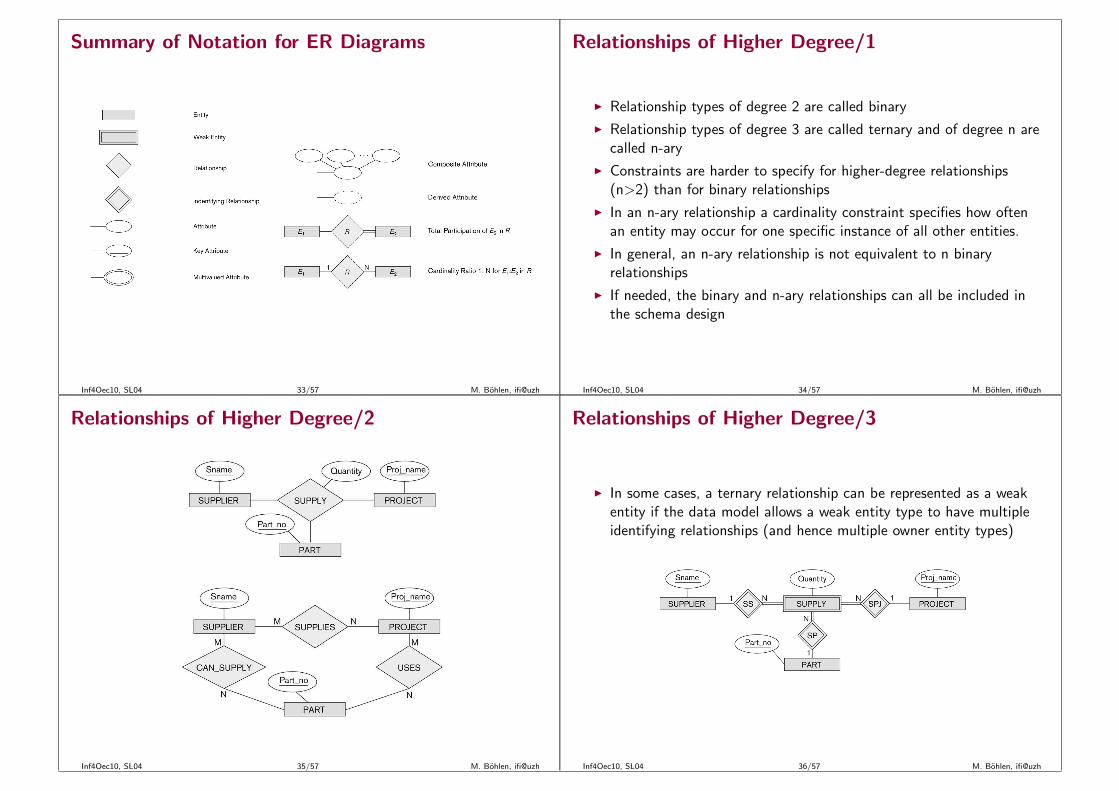
Summary of Notation for ER Diagrams
Inf4Oec10, SL04 33/57 M. Bohlen, ifi@uzh
Relationships of Higher Degree/1
◮ Relationship types of degree 2 are called binary
◮ Relationship types of degree 3 are called ternary and of degree n arecalled n-ary
◮ Constraints are harder to specify for higher-degree relationships(n>2) than for binary relationships
◮ In an n-ary relationship a cardinality constraint specifies how oftenan entity may occur for one specific instance of all other entities.
◮ In general, an n-ary relationship is not equivalent to n binaryrelationships
◮ If needed, the binary and n-ary relationships can all be included inthe schema design
Inf4Oec10, SL04 34/57 M. Bohlen, ifi@uzh
Relationships of Higher Degree/2
Inf4Oec10, SL04 35/57 M. Bohlen, ifi@uzh
Relationships of Higher Degree/3
◮ In some cases, a ternary relationship can be represented as a weakentity if the data model allows a weak entity type to have multipleidentifying relationships (and hence multiple owner entity types)
Inf4Oec10, SL04 36/57 M. Bohlen, ifi@uzh
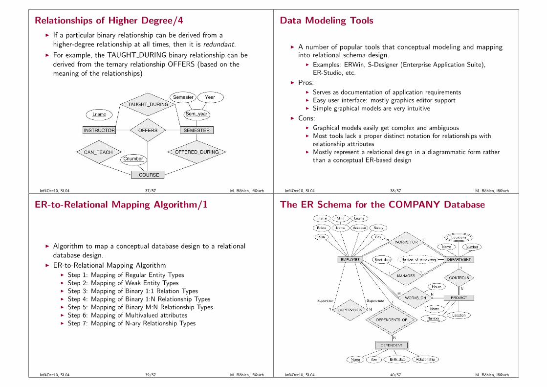
Relationships of Higher Degree/4
◮ If a particular binary relationship can be derived from ahigher-degree relationship at all times, then it is redundant.
◮ For example, the TAUGHT DURING binary relationship can bederived from the ternary relationship OFFERS (based on themeaning of the relationships)
Inf4Oec10, SL04 37/57 M. Bohlen, ifi@uzh
Data Modeling Tools
◮ A number of popular tools that conceptual modeling and mappinginto relational schema design.
◮ Examples: ERWin, S-Designer (Enterprise Application Suite),ER-Studio, etc.
◮ Pros:◮ Serves as documentation of application requirements◮ Easy user interface: mostly graphics editor support◮ Simple graphical models are very intuitive
◮ Cons:◮ Graphical models easily get complex and ambiguous◮ Most tools lack a proper distinct notation for relationships with
relationship attributes◮ Mostly represent a relational design in a diagrammatic form rather
than a conceptual ER-based design
Inf4Oec10, SL04 38/57 M. Bohlen, ifi@uzh
ER-to-Relational Mapping Algorithm/1
◮ Algorithm to map a conceptual database design to a relationaldatabase design.
◮ ER-to-Relational Mapping Algorithm◮ Step 1: Mapping of Regular Entity Types◮ Step 2: Mapping of Weak Entity Types◮ Step 3: Mapping of Binary 1:1 Relation Types◮ Step 4: Mapping of Binary 1:N Relationship Types◮ Step 5: Mapping of Binary M:N Relationship Types◮ Step 6: Mapping of Multivalued attributes◮ Step 7: Mapping of N-ary Relationship Types
Inf4Oec10, SL04 39/57 M. Bohlen, ifi@uzh
The ER Schema for the COMPANY Database
Inf4Oec10, SL04 40/57 M. Bohlen, ifi@uzh
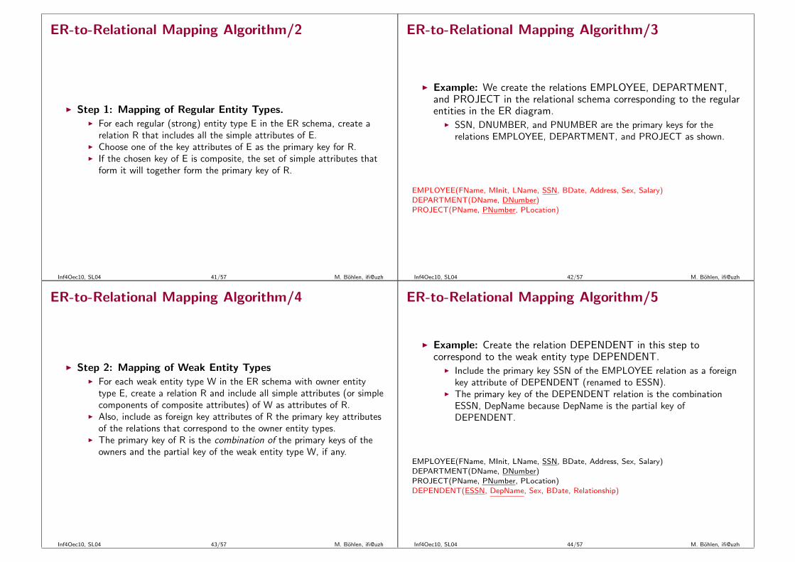
ER-to-Relational Mapping Algorithm/2
◮ Step 1: Mapping of Regular Entity Types.◮ For each regular (strong) entity type E in the ER schema, create a
relation R that includes all the simple attributes of E.◮ Choose one of the key attributes of E as the primary key for R.◮ If the chosen key of E is composite, the set of simple attributes that
form it will together form the primary key of R.
Inf4Oec10, SL04 41/57 M. Bohlen, ifi@uzh
ER-to-Relational Mapping Algorithm/3
◮ Example: We create the relations EMPLOYEE, DEPARTMENT,and PROJECT in the relational schema corresponding to the regularentities in the ER diagram.
◮ SSN, DNUMBER, and PNUMBER are the primary keys for therelations EMPLOYEE, DEPARTMENT, and PROJECT as shown.
EMPLOYEE(FName, MInit, LName, SSN, BDate, Address, Sex, Salary)DEPARTMENT(DName, DNumber)PROJECT(PName, PNumber, PLocation)
Inf4Oec10, SL04 42/57 M. Bohlen, ifi@uzh
ER-to-Relational Mapping Algorithm/4
◮ Step 2: Mapping of Weak Entity Types◮ For each weak entity type W in the ER schema with owner entity
type E, create a relation R and include all simple attributes (or simplecomponents of composite attributes) of W as attributes of R.
◮ Also, include as foreign key attributes of R the primary key attributesof the relations that correspond to the owner entity types.
◮ The primary key of R is the combination of the primary keys of theowners and the partial key of the weak entity type W, if any.
Inf4Oec10, SL04 43/57 M. Bohlen, ifi@uzh
ER-to-Relational Mapping Algorithm/5
◮ Example: Create the relation DEPENDENT in this step tocorrespond to the weak entity type DEPENDENT.
◮ Include the primary key SSN of the EMPLOYEE relation as a foreignkey attribute of DEPENDENT (renamed to ESSN).
◮ The primary key of the DEPENDENT relation is the combinationESSN, DepName because DepName is the partial key ofDEPENDENT.
EMPLOYEE(FName, MInit, LName, SSN, BDate, Address, Sex, Salary)DEPARTMENT(DName, DNumber)PROJECT(PName, PNumber, PLocation)DEPENDENT(ESSN, DepName, Sex, BDate, Relationship)
Inf4Oec10, SL04 44/57 M. Bohlen, ifi@uzh
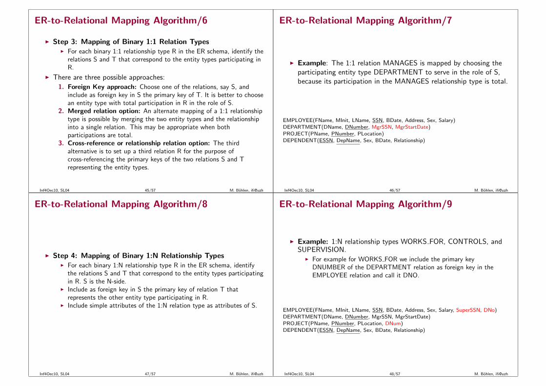
ER-to-Relational Mapping Algorithm/6
◮ Step 3: Mapping of Binary 1:1 Relation Types◮ For each binary 1:1 relationship type R in the ER schema, identify the
relations S and T that correspond to the entity types participating inR.
◮ There are three possible approaches:
1. Foreign Key approach: Choose one of the relations, say S, andinclude as foreign key in S the primary key of T. It is better to choosean entity type with total participation in R in the role of S.
2. Merged relation option: An alternate mapping of a 1:1 relationshiptype is possible by merging the two entity types and the relationshipinto a single relation. This may be appropriate when bothparticipations are total.
3. Cross-reference or relationship relation option: The thirdalternative is to set up a third relation R for the purpose ofcross-referencing the primary keys of the two relations S and Trepresenting the entity types.
Inf4Oec10, SL04 45/57 M. Bohlen, ifi@uzh
ER-to-Relational Mapping Algorithm/7
◮ Example: The 1:1 relation MANAGES is mapped by choosing theparticipating entity type DEPARTMENT to serve in the role of S,because its participation in the MANAGES relationship type is total.
EMPLOYEE(FName, MInit, LName, SSN, BDate, Address, Sex, Salary)DEPARTMENT(DName, DNumber, MgrSSN, MgrStartDate)PROJECT(PName, PNumber, PLocation)DEPENDENT(ESSN, DepName, Sex, BDate, Relationship)
Inf4Oec10, SL04 46/57 M. Bohlen, ifi@uzh
ER-to-Relational Mapping Algorithm/8
◮ Step 4: Mapping of Binary 1:N Relationship Types◮ For each binary 1:N relationship type R in the ER schema, identify
the relations S and T that correspond to the entity types participatingin R. S is the N-side.
◮ Include as foreign key in S the primary key of relation T thatrepresents the other entity type participating in R.
◮ Include simple attributes of the 1:N relation type as attributes of S.
Inf4Oec10, SL04 47/57 M. Bohlen, ifi@uzh
ER-to-Relational Mapping Algorithm/9
◮ Example: 1:N relationship types WORKS FOR, CONTROLS, andSUPERVISION.
◮ For example for WORKS FOR we include the primary keyDNUMBER of the DEPARTMENT relation as foreign key in theEMPLOYEE relation and call it DNO.
EMPLOYEE(FName, MInit, LName, SSN, BDate, Address, Sex, Salary, SuperSSN, DNo)DEPARTMENT(DName, DNumber, MgrSSN, MgrStartDate)PROJECT(PName, PNumber, PLocation, DNum)DEPENDENT(ESSN, DepName, Sex, BDate, Relationship)
Inf4Oec10, SL04 48/57 M. Bohlen, ifi@uzh
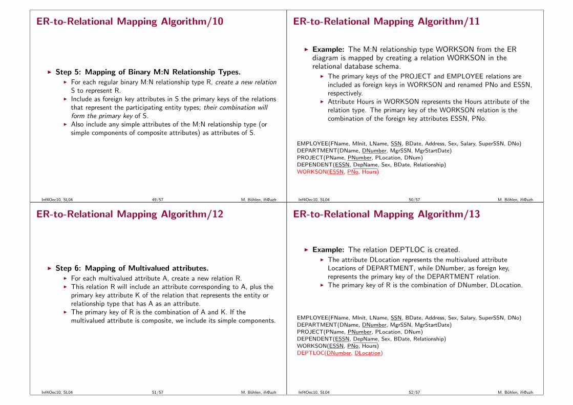
ER-to-Relational Mapping Algorithm/10
◮ Step 5: Mapping of Binary M:N Relationship Types.◮ For each regular binary M:N relationship type R, create a new relation
S to represent R.◮ Include as foreign key attributes in S the primary keys of the relations
that represent the participating entity types; their combination willform the primary key of S.
◮ Also include any simple attributes of the M:N relationship type (orsimple components of composite attributes) as attributes of S.
Inf4Oec10, SL04 49/57 M. Bohlen, ifi@uzh
ER-to-Relational Mapping Algorithm/11
◮ Example: The M:N relationship type WORKSON from the ERdiagram is mapped by creating a relation WORKSON in therelational database schema.
◮ The primary keys of the PROJECT and EMPLOYEE relations areincluded as foreign keys in WORKSON and renamed PNo and ESSN,respectively.
◮ Attribute Hours in WORKSON represents the Hours attribute of therelation type. The primary key of the WORKSON relation is thecombination of the foreign key attributes ESSN, PNo.
EMPLOYEE(FName, MInit, LName, SSN, BDate, Address, Sex, Salary, SuperSSN, DNo)DEPARTMENT(DName, DNumber, MgrSSN, MgrStartDate)PROJECT(PName, PNumber, PLocation, DNum)DEPENDENT(ESSN, DepName, Sex, BDate, Relationship)WORKSON(ESSN, PNo, Hours)
Inf4Oec10, SL04 50/57 M. Bohlen, ifi@uzh
ER-to-Relational Mapping Algorithm/12
◮ Step 6: Mapping of Multivalued attributes.◮ For each multivalued attribute A, create a new relation R.◮ This relation R will include an attribute corresponding to A, plus the
primary key attribute K of the relation that represents the entity orrelationship type that has A as an attribute.
◮ The primary key of R is the combination of A and K. If themultivalued attribute is composite, we include its simple components.
Inf4Oec10, SL04 51/57 M. Bohlen, ifi@uzh
ER-to-Relational Mapping Algorithm/13
◮ Example: The relation DEPTLOC is created.◮ The attribute DLocation represents the multivalued attribute
Locations of DEPARTMENT, while DNumber, as foreign key,represents the primary key of the DEPARTMENT relation.
◮ The primary key of R is the combination of DNumber, DLocation.
EMPLOYEE(FName, MInit, LName, SSN, BDate, Address, Sex, Salary, SuperSSN, DNo)DEPARTMENT(DName, DNumber, MgrSSN, MgrStartDate)PROJECT(PName, PNumber, PLocation, DNum)DEPENDENT(ESSN, DepName, Sex, BDate, Relationship)WORKSON(ESSN, PNo, Hours)DEPTLOC(DNumber, DLocation)
Inf4Oec10, SL04 52/57 M. Bohlen, ifi@uzh
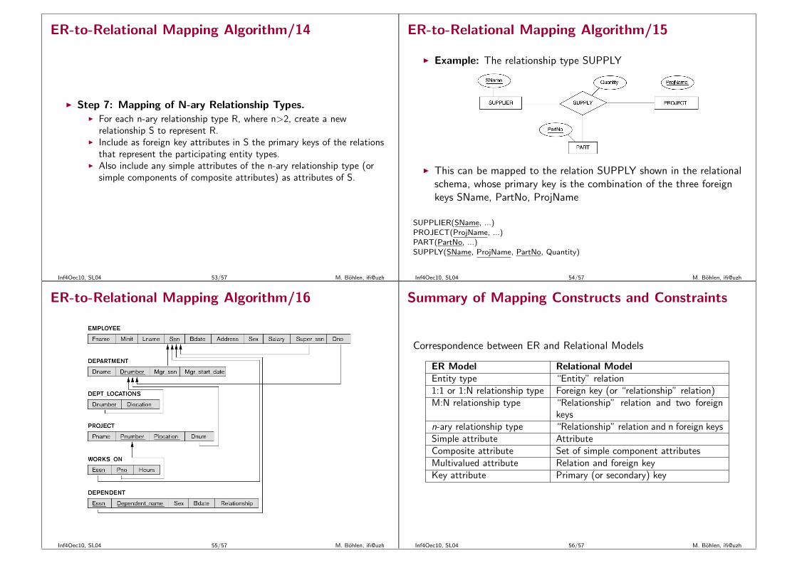
ER-to-Relational Mapping Algorithm/14
◮ Step 7: Mapping of N-ary Relationship Types.◮ For each n-ary relationship type R, where n>2, create a new
relationship S to represent R.◮ Include as foreign key attributes in S the primary keys of the relations
that represent the participating entity types.◮ Also include any simple attributes of the n-ary relationship type (or
simple components of composite attributes) as attributes of S.
Inf4Oec10, SL04 53/57 M. Bohlen, ifi@uzh
ER-to-Relational Mapping Algorithm/15
◮ Example: The relationship type SUPPLY
◮ This can be mapped to the relation SUPPLY shown in the relationalschema, whose primary key is the combination of the three foreignkeys SName, PartNo, ProjName
SUPPLIER(SName, ...)PROJECT(ProjName, ...)PART(PartNo, ...)SUPPLY(SName, ProjName, PartNo, Quantity)
Inf4Oec10, SL04 54/57 M. Bohlen, ifi@uzh
ER-to-Relational Mapping Algorithm/16
Inf4Oec10, SL04 55/57 M. Bohlen, ifi@uzh
Summary of Mapping Constructs and Constraints
Correspondence between ER and Relational Models
ER Model Relational ModelEntity type “Entity” relation1:1 or 1:N relationship type Foreign key (or “relationship” relation)M:N relationship type “Relationship” relation and two foreign
keysn-ary relationship type “Relationship” relation and n foreign keysSimple attribute AttributeComposite attribute Set of simple component attributesMultivalued attribute Relation and foreign keyKey attribute Primary (or secondary) key
Inf4Oec10, SL04 56/57 M. Bohlen, ifi@uzh
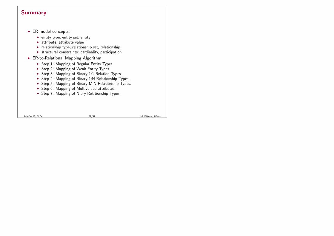
Summary
◮ ER model concepts:◮ entity type, entity set, entity◮ attribute, attribute value◮ relationship type, relationship set, relationship◮ structural constraints: cardinality, participation
◮ ER-to-Relational Mapping Algorithm◮ Step 1: Mapping of Regular Entity Types◮ Step 2: Mapping of Weak Entity Types◮ Step 3: Mapping of Binary 1:1 Relation Types◮ Step 4: Mapping of Binary 1:N Relationship Types.◮ Step 5: Mapping of Binary M:N Relationship Types.◮ Step 6: Mapping of Multivalued attributes.◮ Step 7: Mapping of N-ary Relationship Types.
Inf4Oec10, SL04 57/57 M. Bohlen, ifi@uzh
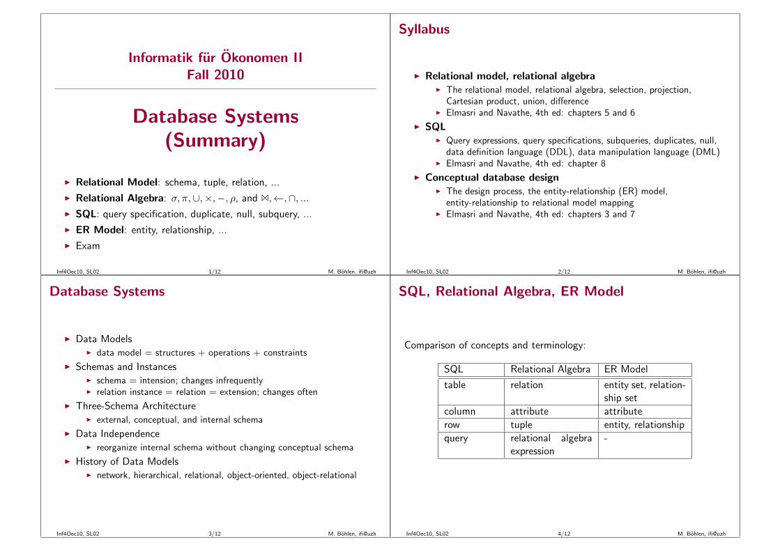
Informatik fur Okonomen IIFall 2010
Database Systems(Summary)
◮ Relational Model: schema, tuple, relation, ...
◮ Relational Algebra: σ, π,∪,×,−, ρ, and 1,←,∩, ...◮ SQL: query specification, duplicate, null, subquery, ...
◮ ER Model: entity, relationship, ...
◮ Exam
Inf4Oec10, SL02 1/12 M. Bohlen, ifi@uzh
Syllabus
◮ Relational model, relational algebra◮ The relational model, relational algebra, selection, projection,
Cartesian product, union, difference◮ Elmasri and Navathe, 4th ed: chapters 5 and 6
◮ SQL◮ Query expressions, query specifications, subqueries, duplicates, null,
data definition language (DDL), data manipulation language (DML)◮ Elmasri and Navathe, 4th ed: chapter 8
◮ Conceptual database design◮ The design process, the entity-relationship (ER) model,
entity-relationship to relational model mapping◮ Elmasri and Navathe, 4th ed: chapters 3 and 7
Inf4Oec10, SL02 2/12 M. Bohlen, ifi@uzh
Database Systems
◮ Data Models◮ data model = structures + operations + constraints
◮ Schemas and Instances◮ schema = intension; changes infrequently◮ relation instance = relation = extension; changes often
◮ Three-Schema Architecture◮ external, conceptual, and internal schema
◮ Data Independence◮ reorganize internal schema without changing conceptual schema
◮ History of Data Models◮ network, hierarchical, relational, object-oriented, object-relational
Inf4Oec10, SL02 3/12 M. Bohlen, ifi@uzh
SQL, Relational Algebra, ER Model
Comparison of concepts and terminology:
SQL Relational Algebra ER Model
table relation entity set, relation-ship set
column attribute attribute
row tuple entity, relationship
query relational algebraexpression
-
Inf4Oec10, SL02 4/12 M. Bohlen, ifi@uzh
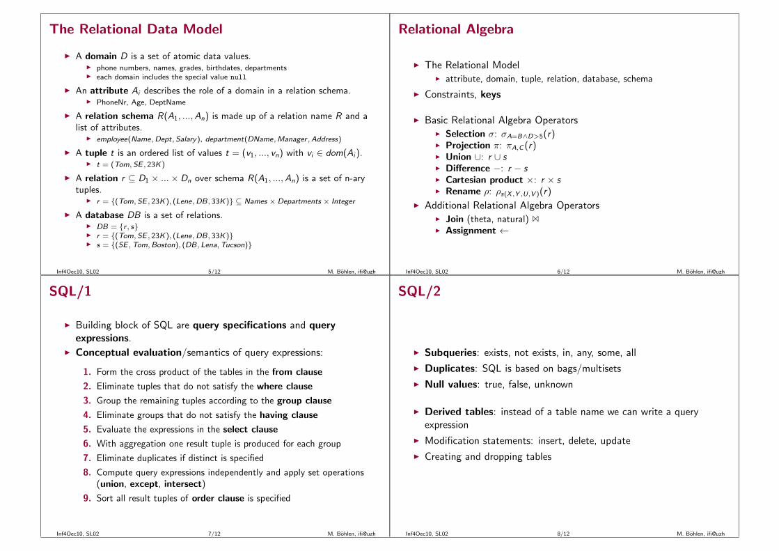
The Relational Data Model
◮ A domain D is a set of atomic data values.◮ phone numbers, names, grades, birthdates, departments◮ each domain includes the special value null
◮ An attribute Ai describes the role of a domain in a relation schema.◮ PhoneNr, Age, DeptName
◮ A relation schema R(A1, ...,An) is made up of a relation name R and alist of attributes.
◮ employee(Name,Dept,Salary), department(DName,Manager ,Address)
◮ A tuple t is an ordered list of values t = (v1, ..., vn) with vi ∈ dom(Ai ).◮ t = (Tom, SE , 23K)
◮ A relation r ⊆ D1 × ...× Dn over schema R(A1, ...,An) is a set of n-arytuples.
◮ r = {(Tom, SE , 23K), (Lene,DB, 33K)} ⊆ Names × Departments × Integer
◮ A database DB is a set of relations.◮ DB = {r , s}◮ r = {(Tom, SE , 23K), (Lene,DB, 33K)}◮ s = {(SE ,Tom,Boston), (DB, Lena,Tucson)}
Inf4Oec10, SL02 5/12 M. Bohlen, ifi@uzh
Relational Algebra
◮ The Relational Model◮ attribute, domain, tuple, relation, database, schema
◮ Constraints, keys
◮ Basic Relational Algebra Operators◮ Selection σ: σA=B∧D>5(r)◮ Projection π: πA,C (r)◮ Union ∪: r ∪ s◮ Difference −: r − s◮ Cartesian product ×: r × s◮ Rename ρ: ρs(X ,Y ,U,V )(r)
◮ Additional Relational Algebra Operators◮ Join (theta, natural) 1◮ Assignment ←
Inf4Oec10, SL02 6/12 M. Bohlen, ifi@uzh
SQL/1
◮ Building block of SQL are query specifications and queryexpressions.
◮ Conceptual evaluation/semantics of query expressions:
1. Form the cross product of the tables in the from clause
2. Eliminate tuples that do not satisfy the where clause
3. Group the remaining tuples according to the group clause
4. Eliminate groups that do not satisfy the having clause
5. Evaluate the expressions in the select clause
6. With aggregation one result tuple is produced for each group
7. Eliminate duplicates if distinct is specified
8. Compute query expressions independently and apply set operations(union, except, intersect)
9. Sort all result tuples of order clause is specified
Inf4Oec10, SL02 7/12 M. Bohlen, ifi@uzh
SQL/2
◮ Subqueries: exists, not exists, in, any, some, all
◮ Duplicates: SQL is based on bags/multisets
◮ Null values: true, false, unknown
◮ Derived tables: instead of a table name we can write a queryexpression
◮ Modification statements: insert, delete, update
◮ Creating and dropping tables
Inf4Oec10, SL02 8/12 M. Bohlen, ifi@uzh
Conceptual Database Design (ER Model)
◮ Basic Entity-Relationship (ER) Model Concepts◮ Entities and attributes, entity types, entity sets◮ Relationships and relationship types◮ Weak entity types
◮ ER-to-Relational Mapping Algorithm◮ Step 1: Mapping of Regular Entity Types◮ Step 2: Mapping of Weak Entity Types◮ Step 3: Mapping of Binary 1:1 Relation Types◮ Step 4: Mapping of Binary 1:N Relationship Types◮ Step 5: Mapping of Binary M:N Relationship Types◮ Step 6: Mapping of Multivalued attributes◮ Step 7: Mapping of N-ary Relationship Types
Inf4Oec10, SL02 9/12 M. Bohlen, ifi@uzh
The Exam (Database Module)
◮ Slides, exercises, solutions are available at the web site
◮ The textbook is Fundamentals of Database Systems by Elmasri andNavathe, 4th edition.
◮ The exercises and examples are important
◮ What is important◮ Being precise about key concepts of relational database systems◮ Being able to apply your knowledge on relevant examples
◮ The final exam is written
◮ The exam is in German; answers can be in German or English
◮ No auxiliary material; use notations from lectures and exercises
◮ Prepare by solving examples as done in exercises
Inf4Oec10, SL02 10/12 M. Bohlen, ifi@uzh
Inf4Oec10, SL02 11/12 M. Bohlen, ifi@uzh
Thanks.
All the best!
Inf4Oec10, SL02 12/12 M. Bohlen, ifi@uzh