Embed Size (px)
Citation preview
DataMining MTAT.03.183(6EAP)Frequentitemsetsand
associationrules
JaakVilo2016Spring
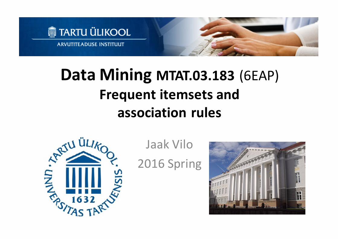
Descriptivedataanalysis
• Aimstosummarisethemainqualitativetraitsofdata.
• Usedmainlyfordiscoveringunderlyingprocessesandrelationsindata.
• Factsarepresentedtogetherwithunderstandableexplanations.
• Usedforexample inmedical,physicalandsocialsciences.
JaakVilo andother authors UT:DataMining 2011 2
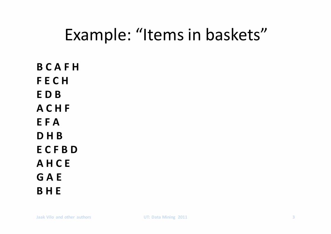
Example:“Itemsinbaskets”
BCAFHFECHEDBACHFEFADHBECFBDAHCEGAEBHE
JaakVilo andother authors UT:DataMining 2011 3
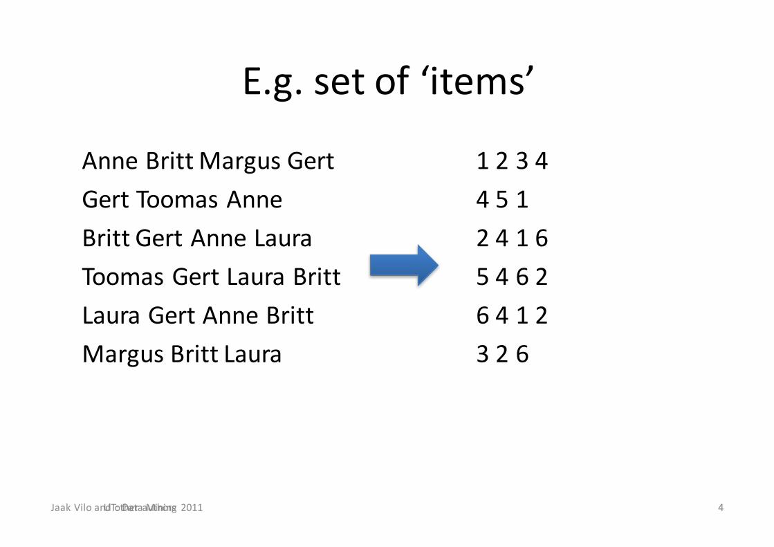
E.g.setof‘items’
AnneBrittMargusGertGertToomasAnneBrittGertAnneLauraToomasGertLauraBrittLauraGertAnneBrittMargusBrittLaura
1234451241654626412326
JaakViloandotherauthorsUT:DataMining2011 4
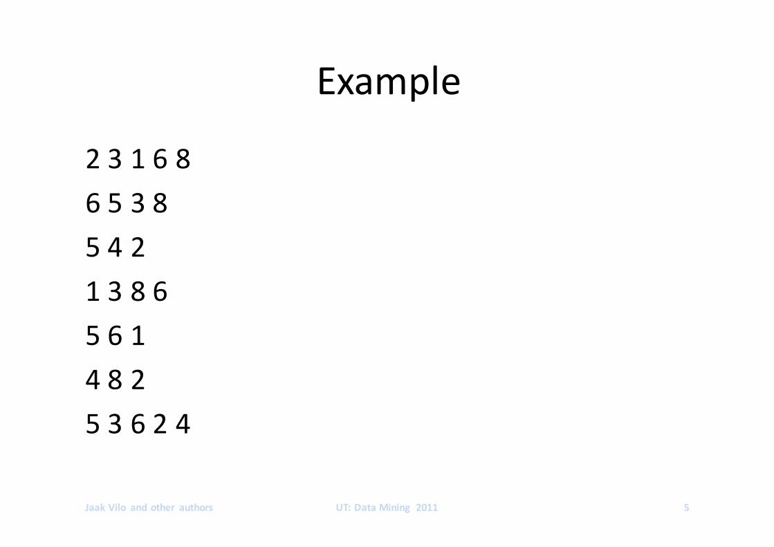
Example
231686538542138656148253624
JaakVilo andother authors UT:DataMining 2011 5
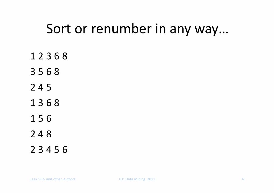
Sortorrenumberinanyway…
123683568245136815624823456
JaakVilo andother authors UT:DataMining 2011 6
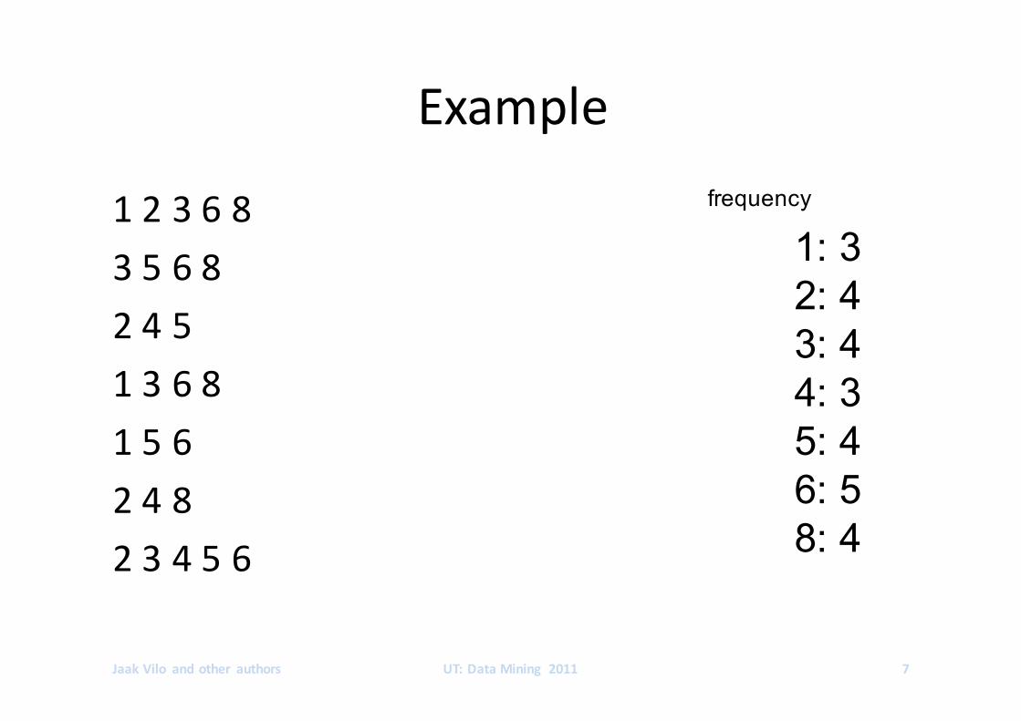
Example
123683568245136815624823456
JaakVilo andother authors UT:DataMining 2011 7
1: 32: 43: 44: 3 5: 4 6: 5 8: 4
frequency
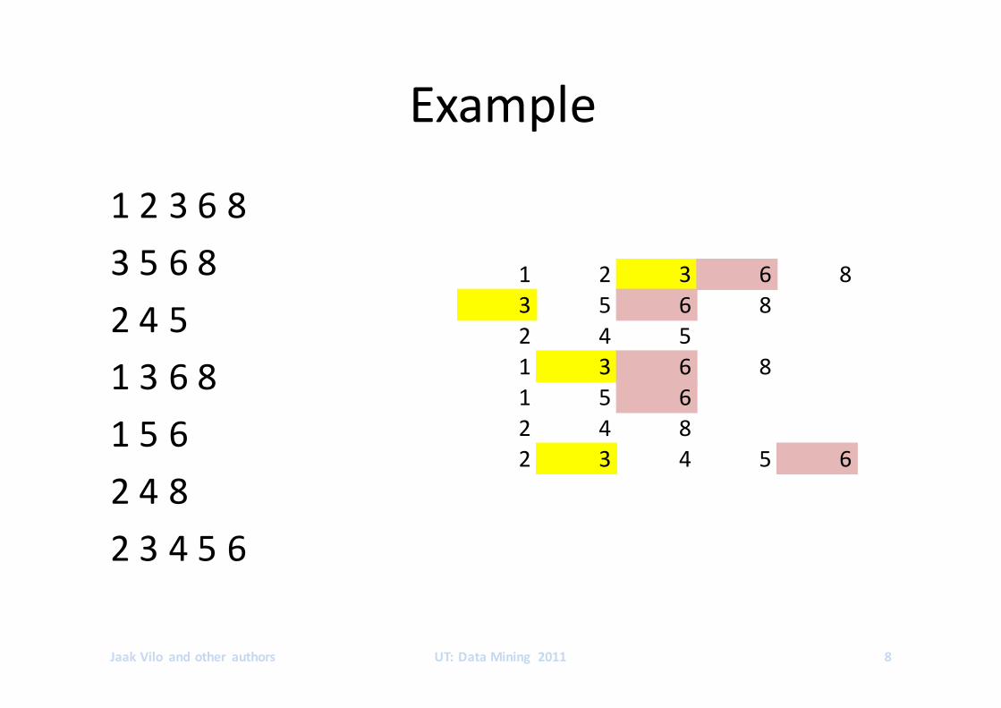
Example
123683568245136815624823456
JaakVilo andother authors UT:DataMining 2011 8
1 2 3 6 83 5 6 82 4 51 3 6 81 5 62 4 82 3 4 5 6
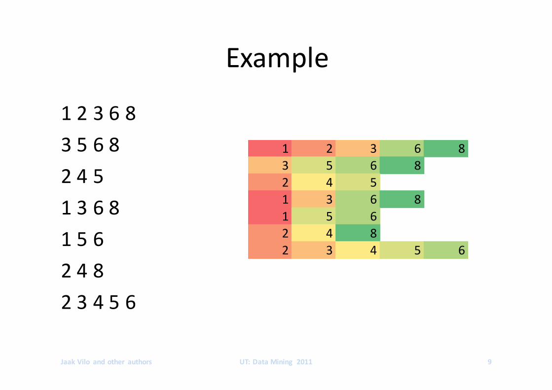
Example
123683568245136815624823456
JaakVilo andother authors UT:DataMining 2011 9
1 2 3 6 83 5 6 82 4 51 3 6 81 5 62 4 82 3 4 5 6

Example
123683568245136815624823456
JaakVilo andother authors UT:DataMining 2011 10
1 2 3 4 5 6 7 81 1 1 1 1 12 1 1 1 13 1 1 14 1 1 1 15 1 1 16 1 1 17 1 1 1 1 1
T-ID
ITEMS
Data Mining Association Analysis: Basic Concepts
and Algorithms
Lecture Notes for Chapter 6
Introduction to Data Miningby
Tan, Steinbach, Kumar
Chapter 6: http://www-users.cs.umn.edu/~kumar/dmbook/ch6.pdf
© Tan,Steinbach, Kumar Introduction to Data Mining 4/18/2004 11
© Tan,Steinbach, Kumar Introduction to Data Mining 4/18/2004 ‹#›
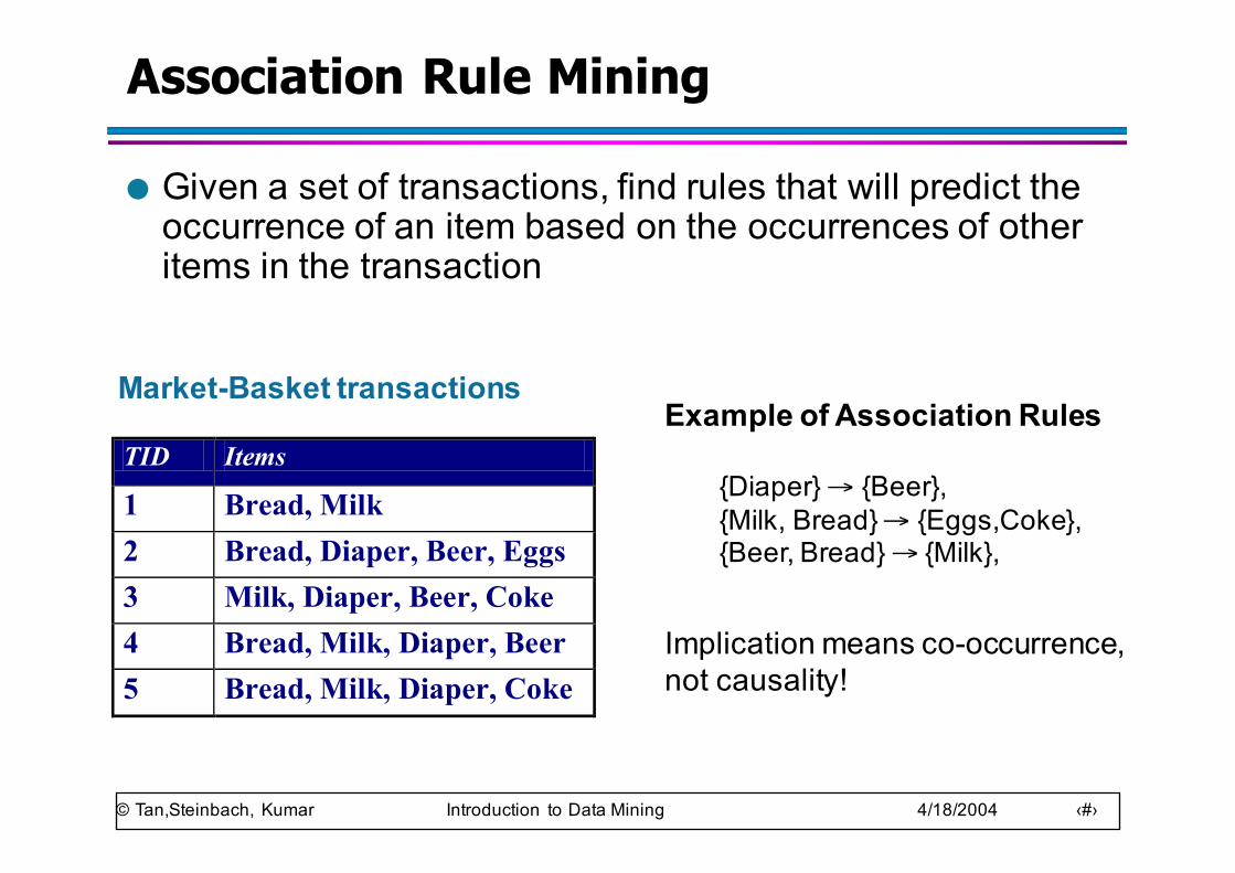
Association Rule Mining
● Given a set of transactions, find rules that will predict the occurrence of an item based on the occurrences of other items in the transaction
Market-Basket transactions
TID Items
1 Bread, Milk
2 Bread, Diaper, Beer, Eggs
3 Milk, Diaper, Beer, Coke 4 Bread, Milk, Diaper, Beer
5 Bread, Milk, Diaper, Coke
Example of Association Rules
{Diaper} → {Beer},{Milk, Bread} → {Eggs,Coke},{Beer, Bread} → {Milk},
Implication means co-occurrence, not causality!
© Tan,Steinbach, Kumar Introduction to Data Mining 4/18/2004 ‹#›
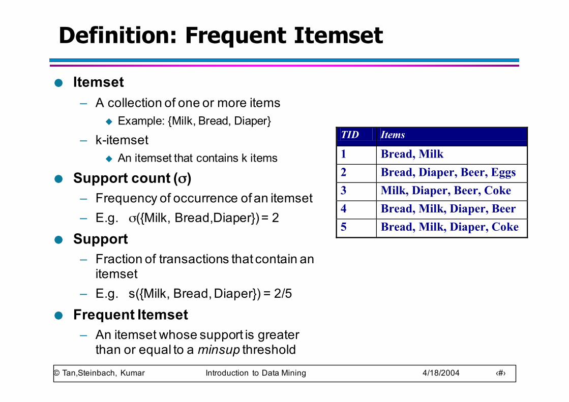
Definition: Frequent Itemset
● Itemset– A collection of one or more items
u Example: {Milk, Bread, Diaper}
– k-itemsetu An itemset that contains k items
● Support count (σ)– Frequency of occurrence of an itemset– E.g. σ({Milk, Bread,Diaper}) = 2
● Support– Fraction of transactions that contain an
itemset– E.g. s({Milk, Bread, Diaper}) = 2/5
● Frequent Itemset– An itemset whose support is greater
than or equal to a minsup threshold
TID Items
1 Bread, Milk
2 Bread, Diaper, Beer, Eggs
3 Milk, Diaper, Beer, Coke 4 Bread, Milk, Diaper, Beer
5 Bread, Milk, Diaper, Coke
© Tan,Steinbach, Kumar Introduction to Data Mining 4/18/2004 ‹#›
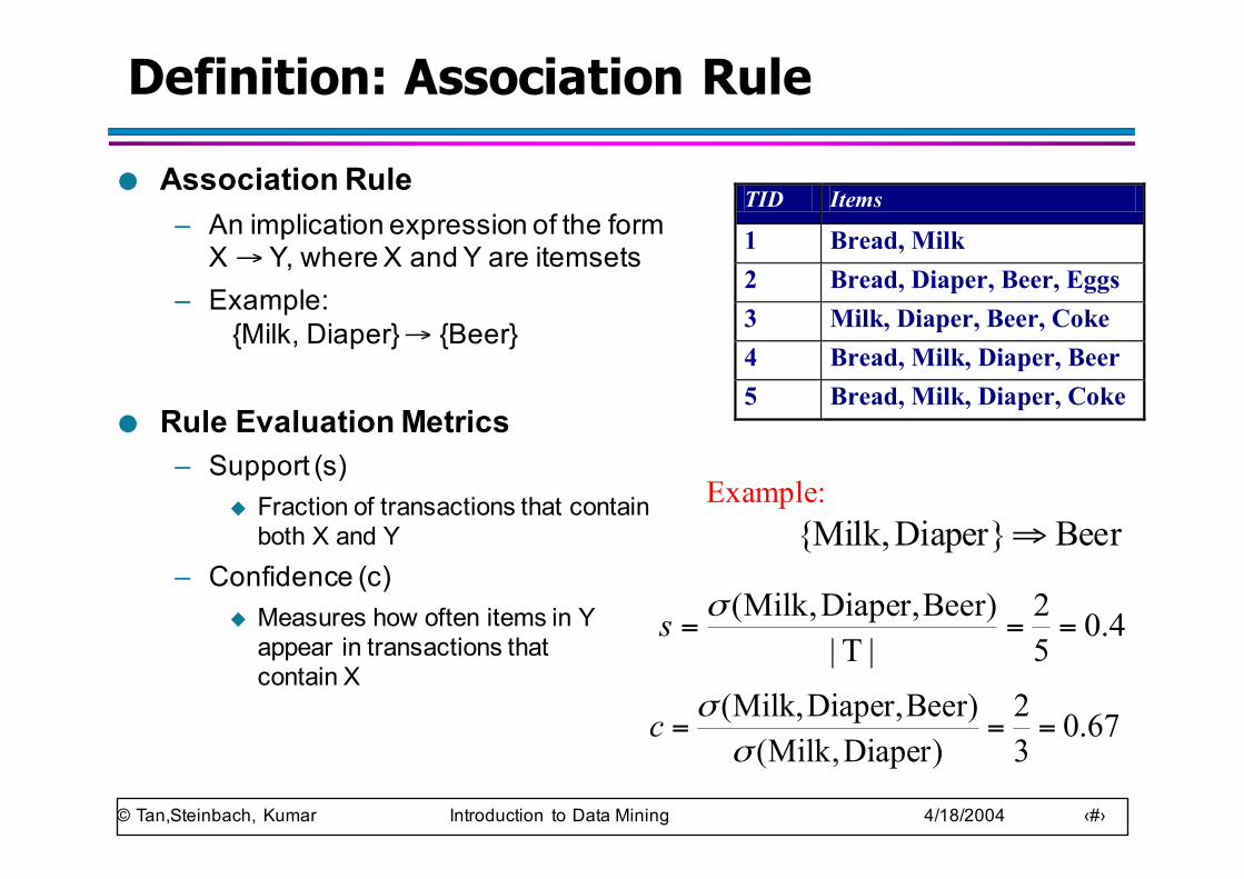
Definition: Association Rule
Example:Beer}Diaper,Milk{ ⇒
4.052
|T|)BeerDiaper,,Milk(
===σs
67.032
)Diaper,Milk()BeerDiaper,Milk,(
===σ
σc
● Association Rule– An implication expression of the form
X → Y, where X and Y are itemsets– Example:
{Milk, Diaper} → {Beer}
● Rule Evaluation Metrics– Support (s)
u Fraction of transactions that contain both X and Y
– Confidence (c)u Measures how often items in Y
appear in transactions thatcontain X
TID Items
1 Bread, Milk
2 Bread, Diaper, Beer, Eggs
3 Milk, Diaper, Beer, Coke 4 Bread, Milk, Diaper, Beer
5 Bread, Milk, Diaper, Coke
© Tan,Steinbach, Kumar Introduction to Data Mining 4/18/2004 ‹#›
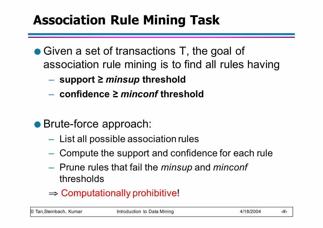
Association Rule Mining Task
● Given a set of transactions T, the goal of association rule mining is to find all rules having
– support ≥ minsup threshold– confidence ≥ minconf threshold
● Brute-force approach:– List all possible association rules– Compute the support and confidence for each rule– Prune rules that fail the minsup and minconf
thresholds⇒ Computationally prohibitive!
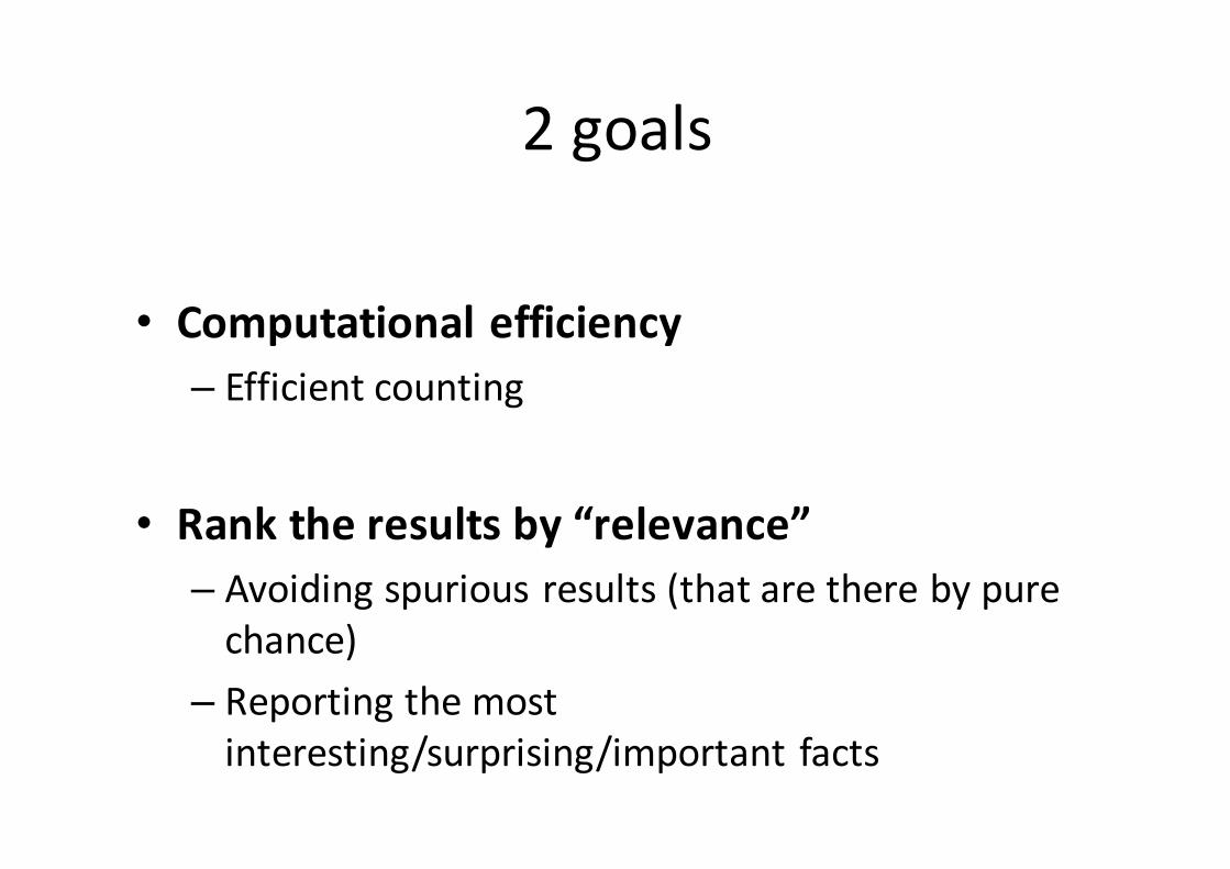
2goals
• Computationalefficiency– Efficientcounting
• Ranktheresultsby“relevance”– Avoidingspuriousresults(thataretherebypurechance)
– Reportingthemostinteresting/surprising/importantfacts
© Tan,Steinbach, Kumar Introduction to Data Mining 4/18/2004 ‹#›
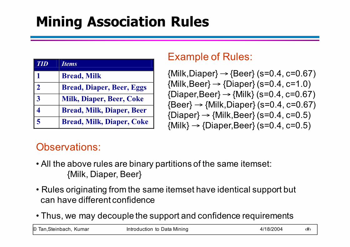
Mining Association Rules
Example of Rules:{Milk,Diaper} → {Beer} (s=0.4, c=0.67){Milk,Beer} → {Diaper} (s=0.4, c=1.0){Diaper,Beer} → {Milk} (s=0.4, c=0.67){Beer} → {Milk,Diaper} (s=0.4, c=0.67) {Diaper} → {Milk,Beer} (s=0.4, c=0.5) {Milk} → {Diaper,Beer} (s=0.4, c=0.5)
TID Items
1 Bread, Milk
2 Bread, Diaper, Beer, Eggs
3 Milk, Diaper, Beer, Coke 4 Bread, Milk, Diaper, Beer
5 Bread, Milk, Diaper, Coke
Observations:• All the above rules are binary partitions of the same itemset:
{Milk, Diaper, Beer}
• Rules originating from the same itemset have identical support butcan have different confidence
• Thus, we may decouple the support and confidence requirements
© Tan,Steinbach, Kumar Introduction to Data Mining 4/18/2004 ‹#›
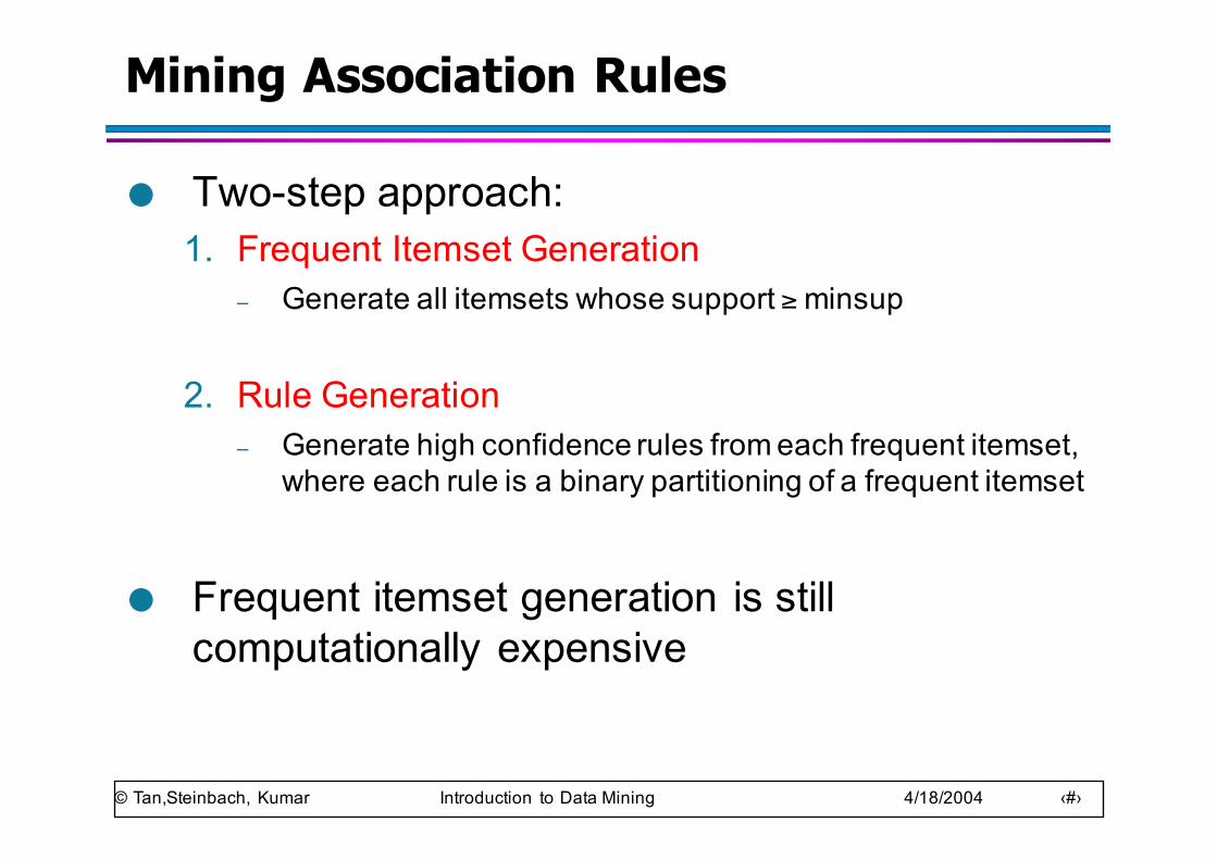
Mining Association Rules
● Two-step approach: 1. Frequent Itemset Generation
– Generate all itemsets whose support ≥minsup
2. Rule Generation– Generate high confidence rules from each frequent itemset,
where each rule is a binary partitioning of a frequent itemset
● Frequent itemset generation is still computationally expensive
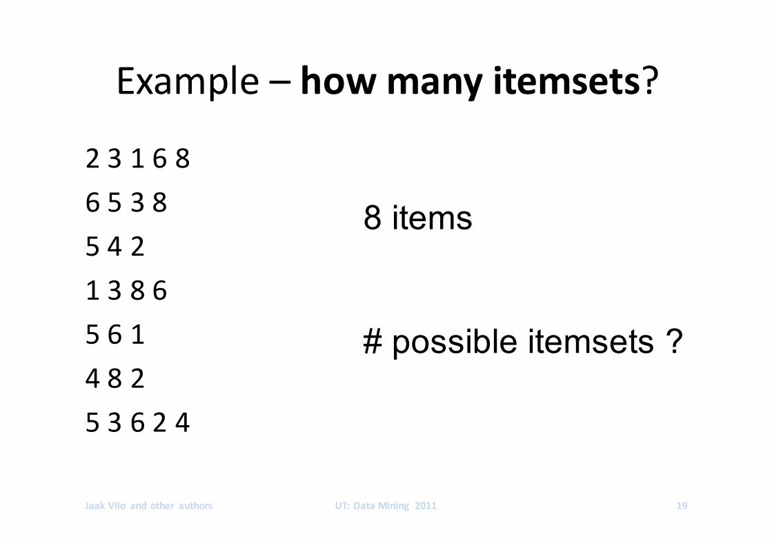
Example– howmanyitemsets?
231686538542138656148253624
JaakVilo andother authors UT:DataMining 2011 19
8 items
# possible itemsets ?
© Tan,Steinbach, Kumar Introduction to Data Mining 4/18/2004 ‹#›
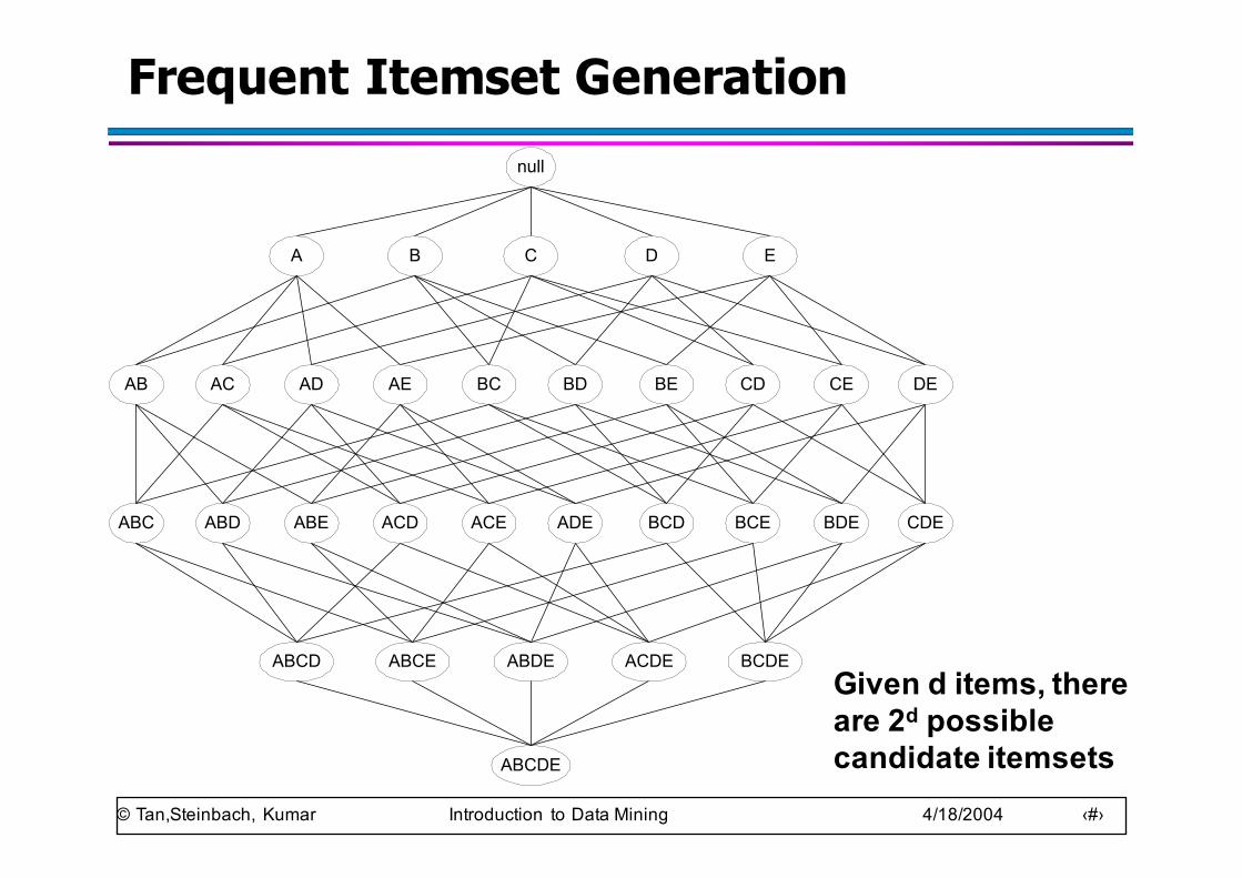
Frequent Itemset Generationnull
AB AC AD AE BC BD BE CD CE DE
A B C D E
ABC ABD ABE ACD ACE ADE BCD BCE BDE CDE
ABCD ABCE ABDE ACDE BCDE
ABCDE
Given d items, there are 2d possible candidate itemsets
© Tan,Steinbach, Kumar Introduction to Data Mining 4/18/2004 ‹#›
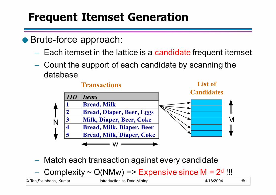
Frequent Itemset Generation
● Brute-force approach: – Each itemset in the lattice is a candidate frequent itemset– Count the support of each candidate by scanning the
database
– Match each transaction against every candidate– Complexity ~ O(NMw) => Expensive since M = 2d !!!
TID Items 1 Bread, Milk 2 Bread, Diaper, Beer, Eggs 3 Milk, Diaper, Beer, Coke 4 Bread, Milk, Diaper, Beer 5 Bread, Milk, Diaper, Coke
N
Transactions List ofCandidates
M
w
© Tan,Steinbach, Kumar Introduction to Data Mining 4/18/2004 ‹#›
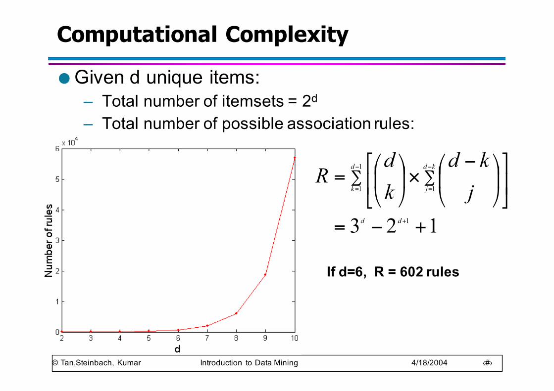
Computational Complexity
● Given d unique items:– Total number of itemsets = 2d
– Total number of possible association rules:
123 1
1
1 1
+−=
⎥⎦
⎤⎢⎣
⎡⎟⎠
⎞⎜⎝
⎛ −×⎟⎠
⎞⎜⎝
⎛=
+
−
=
−
=∑ ∑
dd
d
k
kd
j jkd
kd
R
If d=6, R = 602 rules
Example– counting frequentsubstrings
• Howmany“words”oflengthk,alphabetΣ?
• Howtocountthefrequencyofeverypossiblesubstringinproteinsequences?
• Howtocountallwordsinabook?
• Substringvsregularexpressions
© Tan,Steinbach, Kumar Introduction to Data Mining 4/18/2004 ‹#›
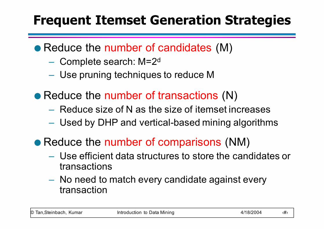
Frequent Itemset Generation Strategies
● Reduce the number of candidates (M)– Complete search: M=2d
– Use pruning techniques to reduce M
● Reduce the number of transactions (N)– Reduce size of N as the size of itemset increases– Used by DHP and vertical-based mining algorithms
● Reduce the number of comparisons (NM)– Use efficient data structures to store the candidates or
transactions– No need to match every candidate against every
transaction
© Tan,Steinbach, Kumar Introduction to Data Mining 4/18/2004 ‹#›
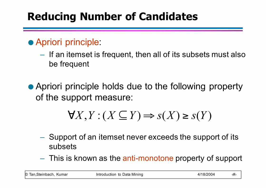
Reducing Number of Candidates
● Apriori principle:– If an itemset is frequent, then all of its subsets must also
be frequent
● Apriori principle holds due to the following property of the support measure:
– Support of an itemset never exceeds the support of its subsets
– This is known as the anti-monotone property of support
)()()(:, YsXsYXYX ≥⇒⊆∀
© Tan,Steinbach, Kumar Introduction to Data Mining 4/18/2004 ‹#›
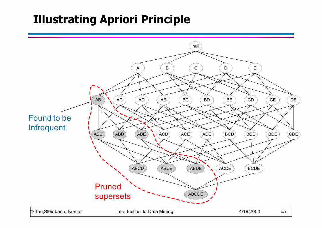
Found to be Infrequent
null
AB AC AD AE BC BD BE CD CE DE
A B C D E
ABC ABD ABE ACD ACE ADE BCD BCE BDE CDE
ABCD ABCE ABDE ACDE BCDE
ABCDE
Illustrating Apriori Principle
null
AB AC AD AE BC BD BE CD CE DE
A B C D E
ABC ABD ABE ACD ACE ADE BCD BCE BDE CDE
ABCD ABCE ABDE ACDE BCDE
ABCDEPruned supersets
© Tan,Steinbach, Kumar Introduction to Data Mining 4/18/2004 ‹#›
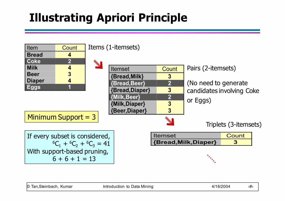
Illustrating Apriori Principle
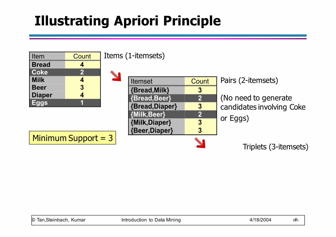
Item CountBread 4Coke 2Milk 4Beer 3Diaper 4Eggs 1
Itemset Count{Bread,Milk} 3{Bread,Beer} 2{Bread,Diaper} 3{Milk,Beer} 2{Milk,Diaper} 3{Beer,Diaper} 3
Itemset Count {Bread,Milk,Diaper} 3
Items (1-itemsets)
Pairs (2-itemsets)
(No need to generatecandidates involving Cokeor Eggs)
Triplets (3-itemsets)Minimum Support = 3
If every subset is considered, 6C1 + 6C2 + 6C3 = 41
With support-based pruning,6 + 6 + 1 = 13
© Tan,Steinbach, Kumar Introduction to Data Mining 4/18/2004 ‹#›
Illustrating Apriori Principle
Item CountBread 4Coke 2Milk 4Beer 3Diaper 4Eggs 1
Itemset Count{Bread,Milk} 3{Bread,Beer} 2{Bread,Diaper} 3{Milk,Beer} 2{Milk,Diaper} 3{Beer,Diaper} 3
Itemset Count {Bread,Milk,Diaper} 3
Items (1-itemsets)
Pairs (2-itemsets)
(No need to generatecandidates involving Cokeor Eggs)
Triplets (3-itemsets)Minimum Support = 3
If every subset is considered, 6C1 + 6C2 + 6C3 = 41
With support-based pruning,6 + 6 + 1 = 13
© Tan,Steinbach, Kumar Introduction to Data Mining 4/18/2004 ‹#›
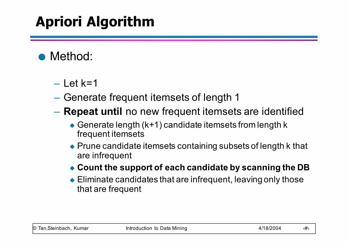
Apriori Algorithm
● Method:
– Let k=1– Generate frequent itemsets of length 1– Repeat until no new frequent itemsets are identified
u Generate length (k+1) candidate itemsets from length k frequent itemsets
u Prune candidate itemsets containing subsets of length k that are infrequent
u Count the support of each candidate by scanning the DBu Eliminate candidates that are infrequent, leaving only those
that are frequent
© Tan,Steinbach, Kumar Introduction to Data Mining 4/18/2004 ‹#›
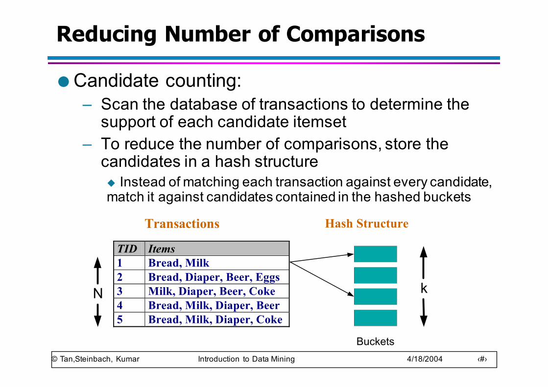
Reducing Number of Comparisons
● Candidate counting:– Scan the database of transactions to determine the
support of each candidate itemset– To reduce the number of comparisons, store the
candidates in a hash structureu Instead of matching each transaction against every candidate, match it against candidates contained in the hashed buckets
TID Items 1 Bread, Milk 2 Bread, Diaper, Beer, Eggs 3 Milk, Diaper, Beer, Coke 4 Bread, Milk, Diaper, Beer 5 Bread, Milk, Diaper, Coke
N
Transactions Hash Structure
k
Buckets
© Tan,Steinbach, Kumar Introduction to Data Mining 4/18/2004 ‹#›
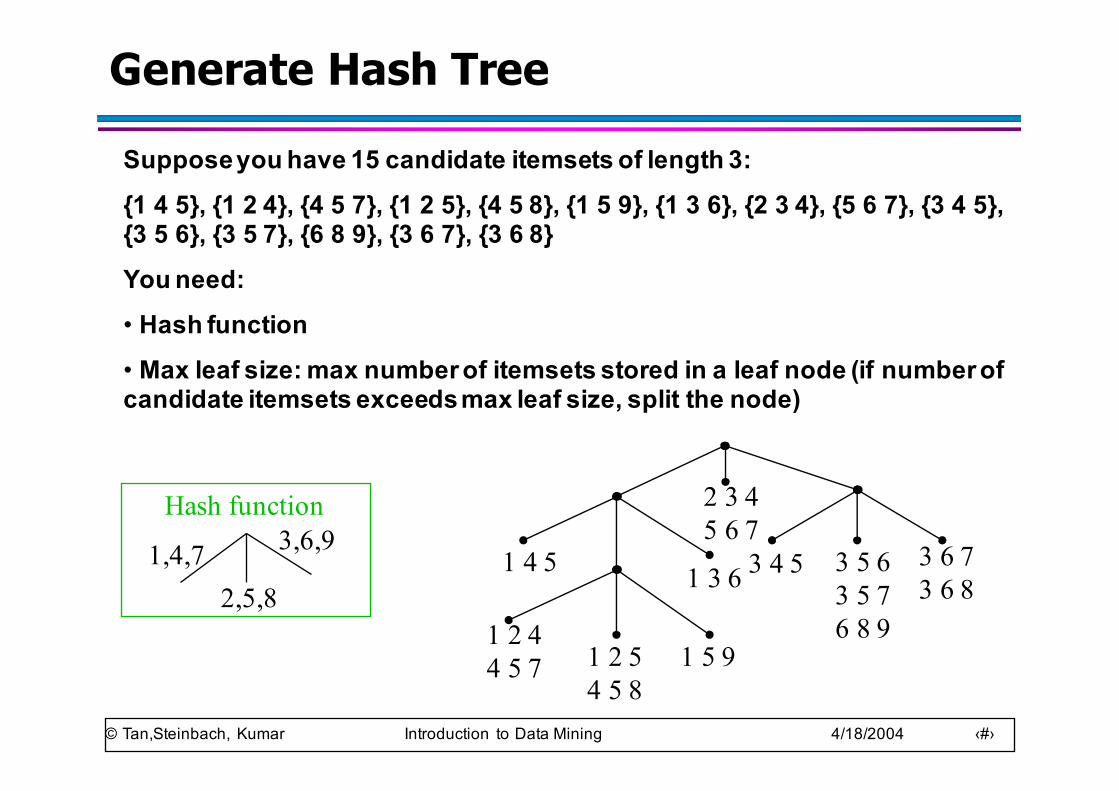
Generate Hash Tree
2 3 45 6 7
1 4 5 1 3 6
1 2 44 5 7 1 2 5
4 5 81 5 9
3 4 5 3 5 63 5 76 8 9
3 6 73 6 8
1,4,72,5,8
3,6,9Hash function
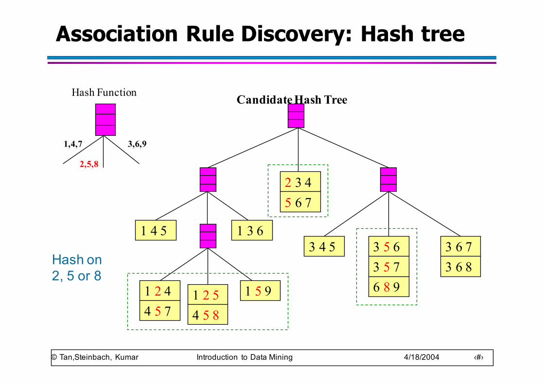
Suppose you have 15 candidate itemsets of length 3: {1 4 5}, {1 2 4}, {4 5 7}, {1 2 5}, {4 5 8}, {1 5 9}, {1 3 6}, {2 3 4}, {5 6 7}, {3 4 5}, {3 5 6}, {3 5 7}, {6 8 9}, {3 6 7}, {3 6 8}You need:• Hash function • Max leaf size: max number of itemsets stored in a leaf node (if number of candidate itemsets exceeds max leaf size, split the node)

© Tan,Steinbach, Kumar Introduction to Data Mining 4/18/2004 ‹#›
Association Rule Discovery: Hash tree
1 5 9
1 4 5 1 3 63 4 5 3 6 7
3 6 83 5 63 5 76 8 9
2 3 45 6 7
1 2 44 5 7
1 2 54 5 8
1,4,7
2,5,8
3,6,9
Hash Function Candidate Hash Tree
Hash on 1, 4 or 7
© Tan,Steinbach, Kumar Introduction to Data Mining 4/18/2004 ‹#›
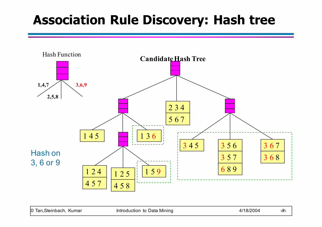
Association Rule Discovery: Hash tree
1 5 9
1 4 5 1 3 63 4 5 3 6 7
3 6 83 5 63 5 76 8 9
2 3 45 6 7
1 2 44 5 7
1 2 54 5 8
1,4,7
2,5,8
3,6,9
Hash Function Candidate Hash Tree
Hash on 2, 5 or 8
© Tan,Steinbach, Kumar Introduction to Data Mining 4/18/2004 ‹#›
Association Rule Discovery: Hash tree
1 5 9
1 4 5 1 3 63 4 5 3 6 7
3 6 83 5 63 5 76 8 9
2 3 45 6 7
1 2 44 5 7
1 2 54 5 8
1,4,7
2,5,8
3,6,9
Hash Function Candidate Hash Tree
Hash on 3, 6 or 9
© Tan,Steinbach, Kumar Introduction to Data Mining 4/18/2004 ‹#›
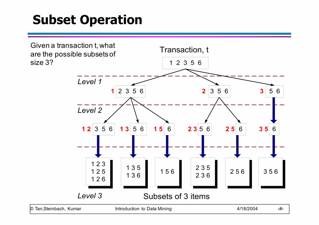
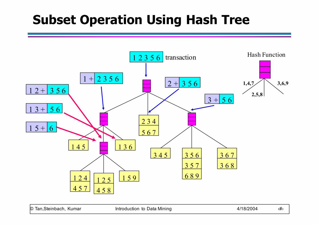
Subset Operation
1 2 3 5 6
Transaction, t
2 3 5 61 3 5 62
5 61 33 5 61 2 61 5 5 62 3 62 5
5 63
1 2 31 2 51 2 6
1 3 51 3 6 1 5 6 2 3 5
2 3 6 2 5 6 3 5 6
Subsets of 3 items
Level 1
Level 2
Level 3
63 5
Given a transaction t, what are the possible subsets of size 3?
© Tan,Steinbach, Kumar Introduction to Data Mining 4/18/2004 ‹#›
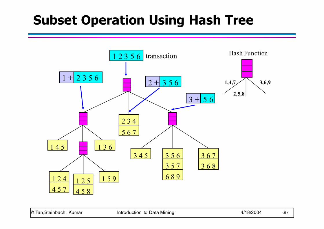
Subset Operation Using Hash Tree
1 5 9
1 4 5 1 3 63 4 5 3 6 7
3 6 83 5 63 5 76 8 9
2 3 45 6 7
1 2 44 5 7
1 2 54 5 8
1 2 3 5 6
1 + 2 3 5 6 3 5 62 +
5 63 +
1,4,7
2,5,8
3,6,9
Hash Functiontransaction
© Tan,Steinbach, Kumar Introduction to Data Mining 4/18/2004 ‹#›
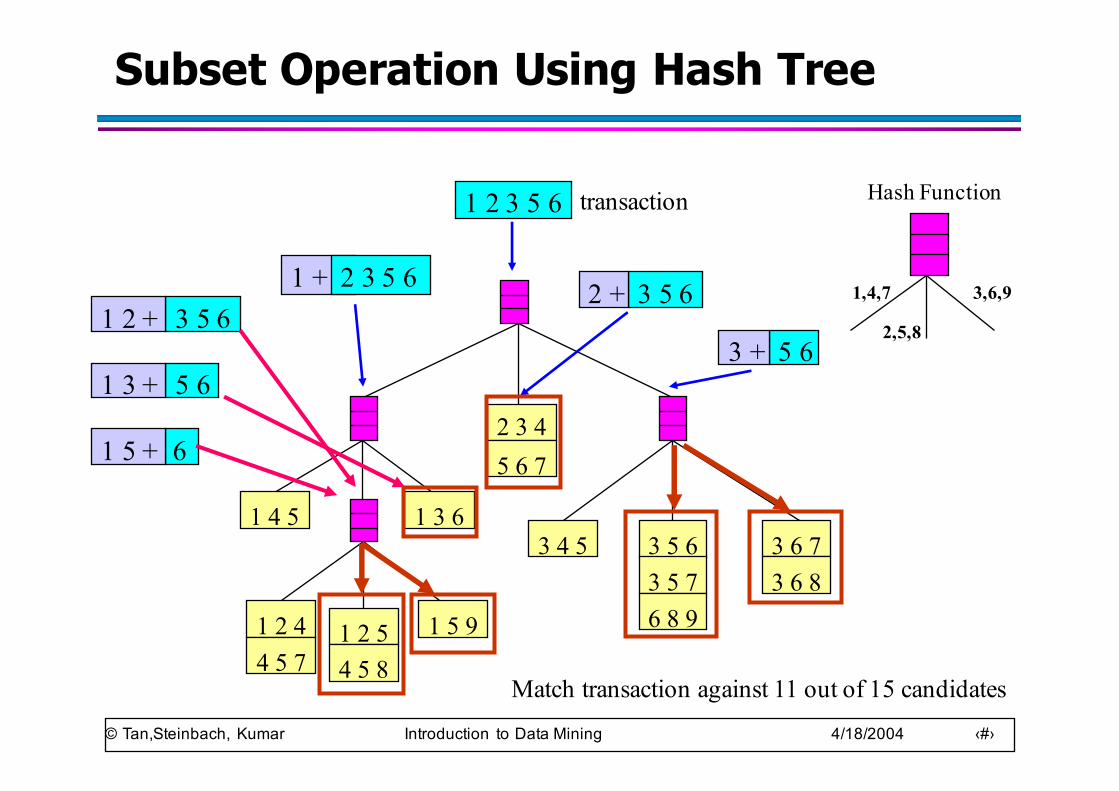
Subset Operation Using Hash Tree
1 5 9
1 4 5 1 3 63 4 5 3 6 7
3 6 83 5 63 5 76 8 9
2 3 45 6 7
1 2 44 5 7
1 2 54 5 8
1,4,7
2,5,8
3,6,9
Hash Function1 2 3 5 6
3 5 61 2 +
5 61 3 +
61 5 +
3 5 62 +
5 63 +
1 + 2 3 5 6
transaction
© Tan,Steinbach, Kumar Introduction to Data Mining 4/18/2004 ‹#›
Subset Operation Using Hash Tree
1 5 9
1 4 5 1 3 63 4 5 3 6 7
3 6 83 5 63 5 76 8 9
2 3 45 6 7
1 2 44 5 7
1 2 54 5 8
1,4,7
2,5,8
3,6,9
Hash Function1 2 3 5 6
3 5 61 2 +
5 61 3 +
61 5 +
3 5 62 +
5 63 +
1 + 2 3 5 6
transaction
Match transaction against 11 out of 15 candidates
© Tan,Steinbach, Kumar Introduction to Data Mining 4/18/2004 ‹#›
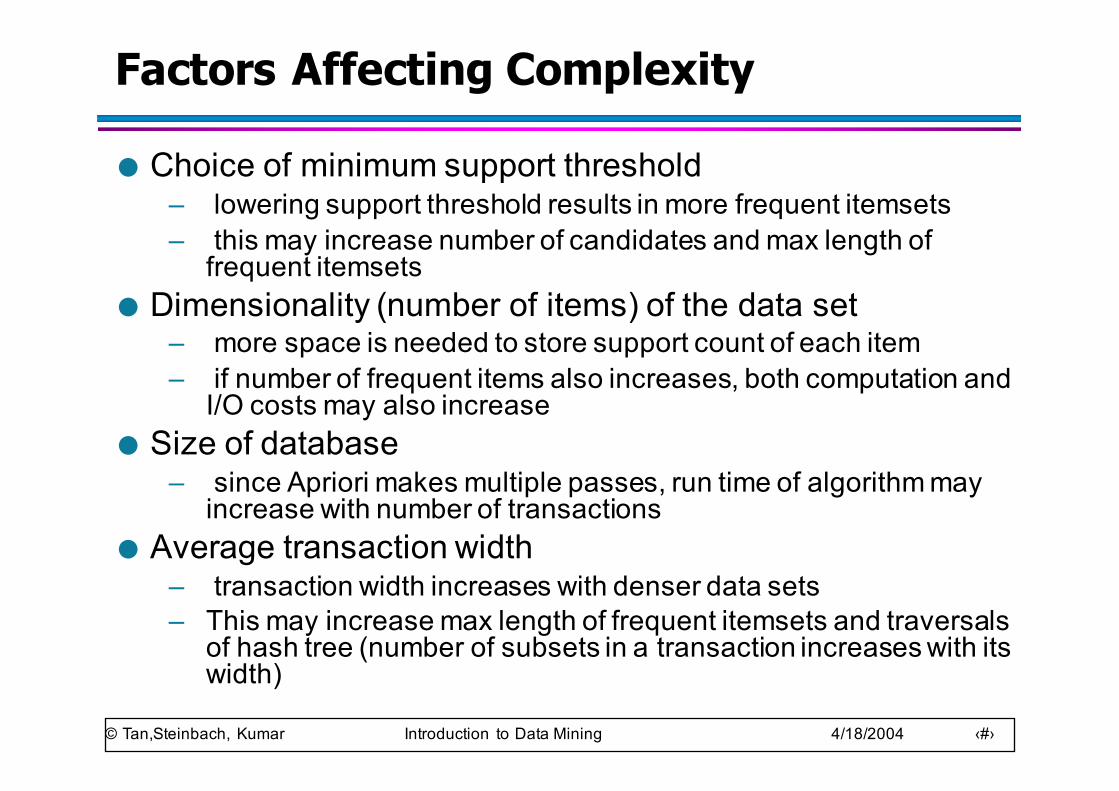
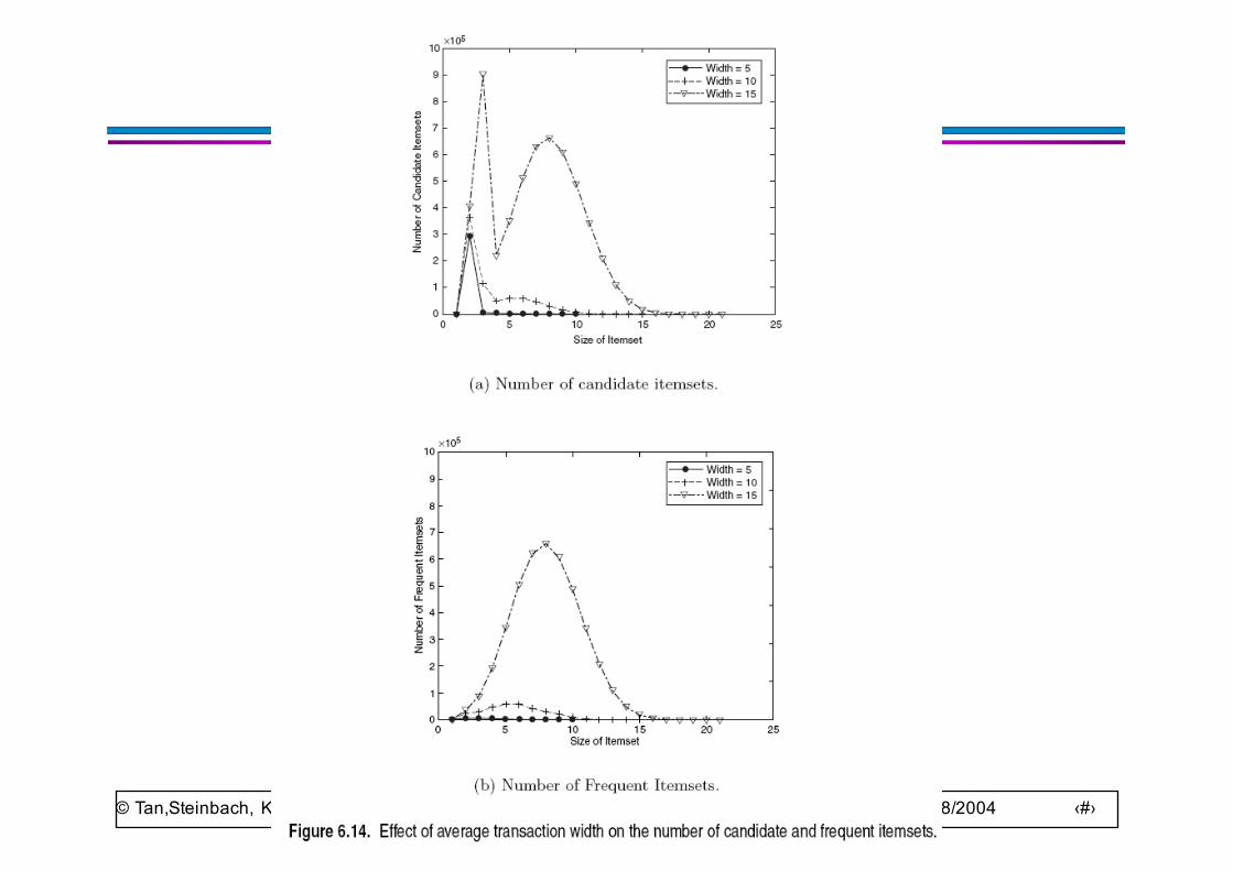
Factors Affecting Complexity
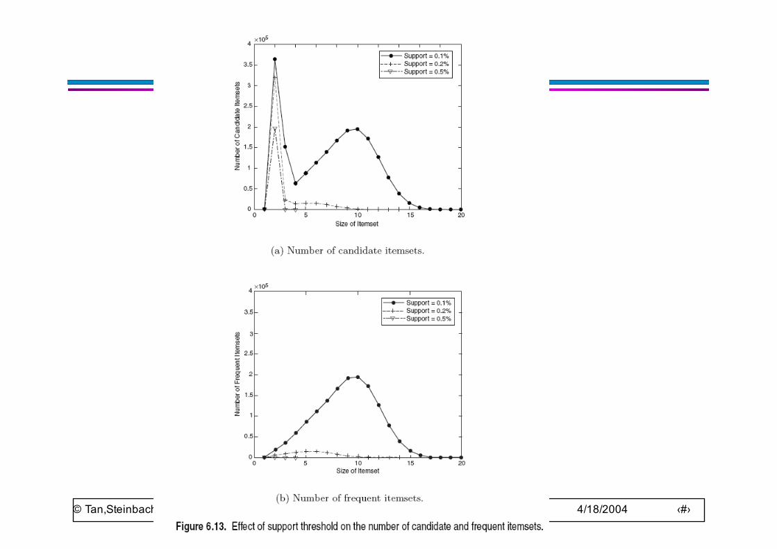
● Choice of minimum support threshold– lowering support threshold results in more frequent itemsets– this may increase number of candidates and max length of
frequent itemsets● Dimensionality (number of items) of the data set
– more space is needed to store support count of each item– if number of frequent items also increases, both computation and
I/O costs may also increase● Size of database
– since Apriori makes multiple passes, run time of algorithm may increase with number of transactions
● Average transaction width– transaction width increases with denser data sets– This may increase max length of frequent itemsets and traversals
of hash tree (number of subsets in a transaction increases with its width)
© Tan,Steinbach, Kumar Introduction to Data Mining 4/18/2004 ‹#›
© Tan,Steinbach, Kumar Introduction to Data Mining 4/18/2004 ‹#›
© Tan,Steinbach, Kumar Introduction to Data Mining 4/18/2004 ‹#›
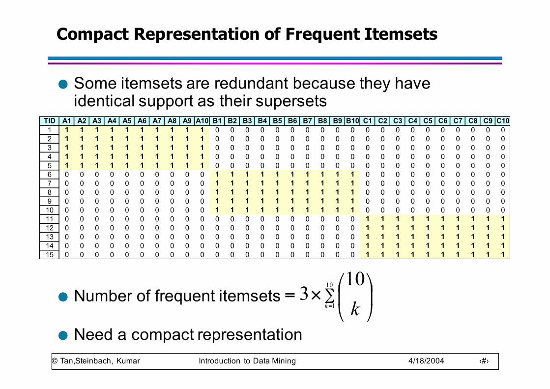
Compact Representation of Frequent Itemsets
● Some itemsets are redundant because they have identical support as their supersets
● Number of frequent itemsets
● Need a compact representation
TID A1 A2 A3 A4 A5 A6 A7 A8 A9 A10 B1 B2 B3 B4 B5 B6 B7 B8 B9 B10 C1 C2 C3 C4 C5 C6 C7 C8 C9 C101 1 1 1 1 1 1 1 1 1 1 0 0 0 0 0 0 0 0 0 0 0 0 0 0 0 0 0 0 0 02 1 1 1 1 1 1 1 1 1 1 0 0 0 0 0 0 0 0 0 0 0 0 0 0 0 0 0 0 0 03 1 1 1 1 1 1 1 1 1 1 0 0 0 0 0 0 0 0 0 0 0 0 0 0 0 0 0 0 0 04 1 1 1 1 1 1 1 1 1 1 0 0 0 0 0 0 0 0 0 0 0 0 0 0 0 0 0 0 0 05 1 1 1 1 1 1 1 1 1 1 0 0 0 0 0 0 0 0 0 0 0 0 0 0 0 0 0 0 0 06 0 0 0 0 0 0 0 0 0 0 1 1 1 1 1 1 1 1 1 1 0 0 0 0 0 0 0 0 0 07 0 0 0 0 0 0 0 0 0 0 1 1 1 1 1 1 1 1 1 1 0 0 0 0 0 0 0 0 0 08 0 0 0 0 0 0 0 0 0 0 1 1 1 1 1 1 1 1 1 1 0 0 0 0 0 0 0 0 0 09 0 0 0 0 0 0 0 0 0 0 1 1 1 1 1 1 1 1 1 1 0 0 0 0 0 0 0 0 0 010 0 0 0 0 0 0 0 0 0 0 1 1 1 1 1 1 1 1 1 1 0 0 0 0 0 0 0 0 0 011 0 0 0 0 0 0 0 0 0 0 0 0 0 0 0 0 0 0 0 0 1 1 1 1 1 1 1 1 1 112 0 0 0 0 0 0 0 0 0 0 0 0 0 0 0 0 0 0 0 0 1 1 1 1 1 1 1 1 1 113 0 0 0 0 0 0 0 0 0 0 0 0 0 0 0 0 0 0 0 0 1 1 1 1 1 1 1 1 1 114 0 0 0 0 0 0 0 0 0 0 0 0 0 0 0 0 0 0 0 0 1 1 1 1 1 1 1 1 1 115 0 0 0 0 0 0 0 0 0 0 0 0 0 0 0 0 0 0 0 0 1 1 1 1 1 1 1 1 1 1
∑=
⎟⎠
⎞⎜⎝
⎛×=
10
1
103
k k

© Tan,Steinbach, Kumar Introduction to Data Mining 4/18/2004 ‹#›
Maximal Frequent Itemset
null
AB AC AD AE BC BD BE CD CE DE
A B C D E
ABC ABD ABE ACD ACE ADE BCD BCE BDE CDE
ABCD ABCE ABDE ACDE BCDE
ABCDE
BorderInfrequent Itemsets
Maximal Itemsets
An itemset is maximal frequent if none of its immediate supersets is frequent
© Tan,Steinbach, Kumar Introduction to Data Mining 4/18/2004 ‹#›
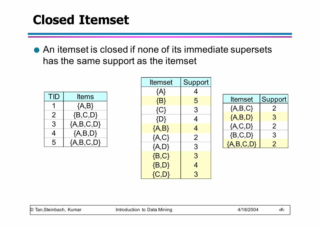
Closed Itemset
● An itemset is closed if none of its immediate supersets has the same support as the itemset
TID Items1 {A,B}2 {B,C,D}3 {A,B,C,D}4 {A,B,D}5 {A,B,C,D}
Itemset Support{A} 4{B} 5{C} 3{D} 4{A,B} 4{A,C} 2{A,D} 3{B,C} 3{B,D} 4{C,D} 3
Itemset Support{A,B,C} 2{A,B,D} 3{A,C,D} 2{B,C,D} 3{A,B,C,D} 2
© Tan,Steinbach, Kumar Introduction to Data Mining 4/18/2004 ‹#›
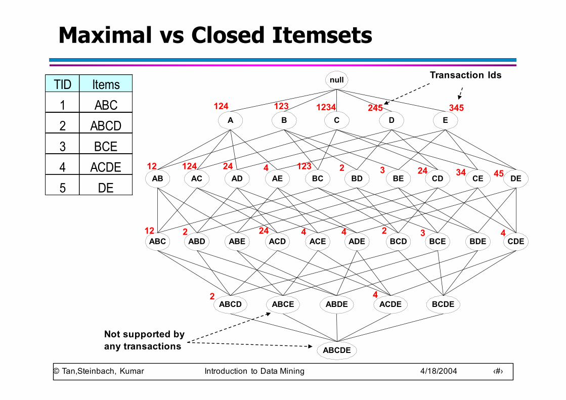
Maximal vs Closed Itemsets
TID Items1 ABC2 ABCD3 BCE4 ACDE5 DE
null
AB AC AD AE BC BD BE CD CE DE
A B C D E
ABC ABD ABE ACD ACE ADE BCD BCE BDE CDE
ABCD ABCE ABDE ACDE BCDE
ABCDE
124 123 1234 245 345
12 124 24 4 123 2 3 24 34 45
12 2 24 4 4 2 3 4
2 4
Transaction Ids
Not supported by any transactions
© Tan,Steinbach, Kumar Introduction to Data Mining 4/18/2004 ‹#›
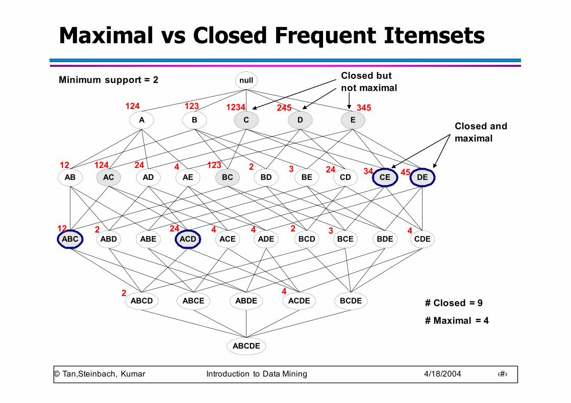
Maximal vs Closed Frequent Itemsetsnull
AB AC AD AE BC BD BE CD CE DE
A B C D E
ABC ABD ABE ACD ACE ADE BCD BCE BDE CDE
ABCD ABCE ABDE ACDE BCDE
ABCDE
124 123 1234 245 345
12 124 24 4 123 2 3 24 34 45
12 2 24 4 4 2 3 4
2 4
Minimum support = 2
# Closed = 9
# Maximal = 4
Closed and maximal
Closed but not maximal
© Tan,Steinbach, Kumar Introduction to Data Mining 4/18/2004 ‹#›
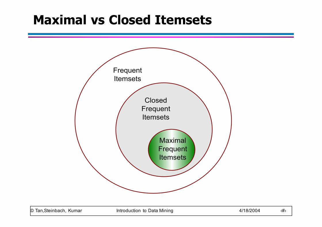
Maximal vs Closed Itemsets
FrequentItemsets
ClosedFrequentItemsets
MaximalFrequentItemsets
© Tan,Steinbach, Kumar Introduction to Data Mining 4/18/2004 ‹#›
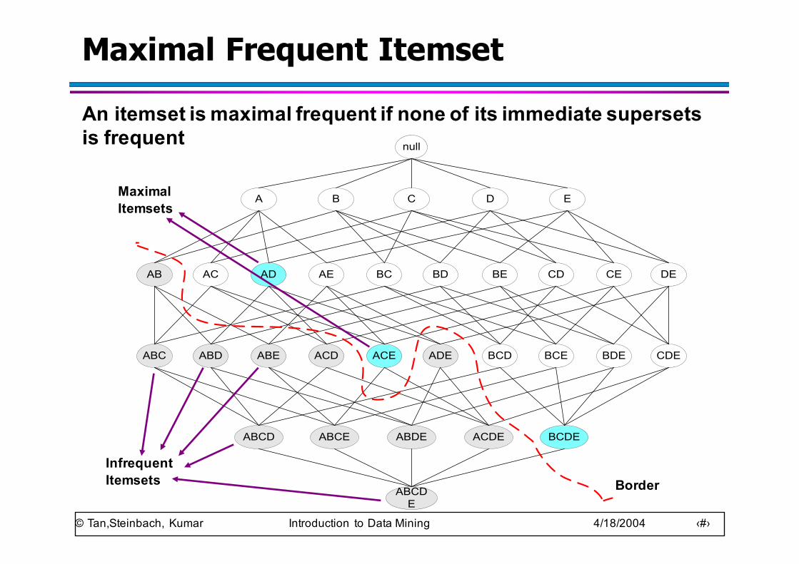
Maximal Frequent Itemset
null
AB AC AD AE BC BD BE CD CE DE
A B C D E
ABC ABD ABE ACD ACE ADE BCD BCE BDE CDE
ABCD ABCE ABDE ACDE BCDE
ABCDE
BorderInfrequent Itemsets
Maximal Itemsets
An itemset is maximal frequent if none of its immediate supersets is frequent
© Tan,Steinbach, Kumar Introduction to Data Mining 4/18/2004 ‹#›
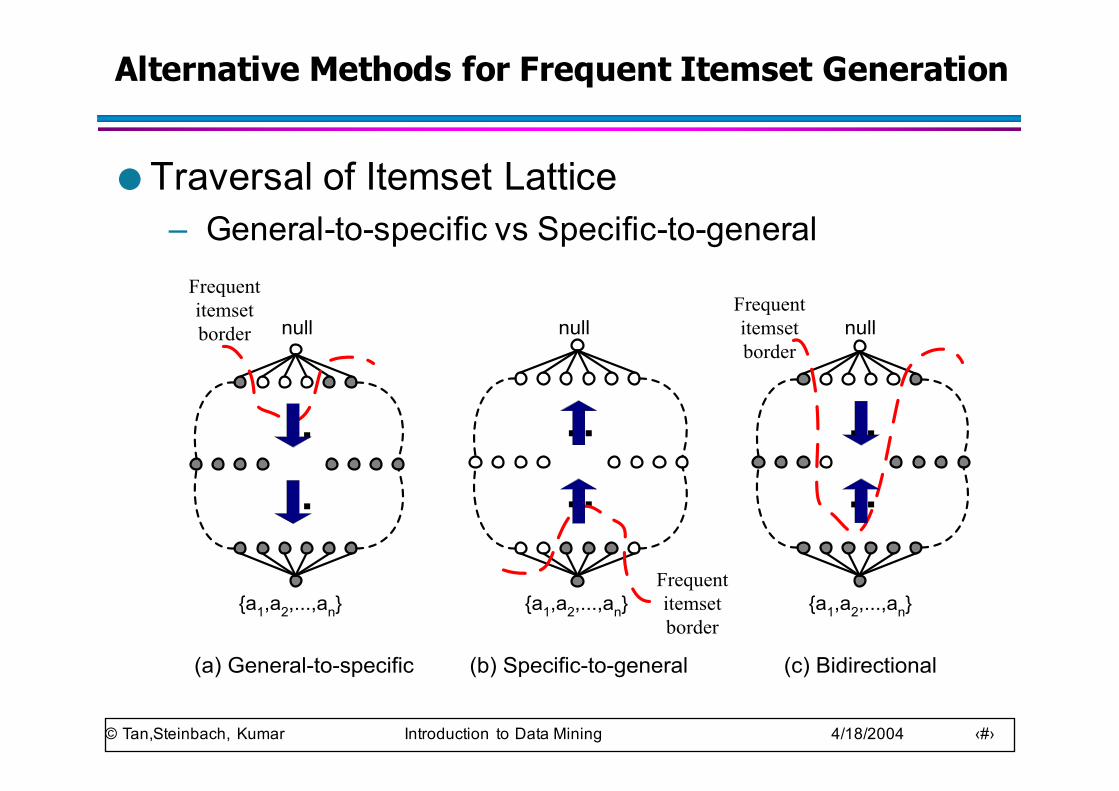
Alternative Methods for Frequent Itemset Generation
● Traversal of Itemset Lattice– General-to-specific vs Specific-to-generalFrequentitemsetborder null
{a1,a2,...,an}
(a) General-to-specific
null
{a1,a2,...,an}
Frequentitemsetborder
(b) Specific-to-general
..
......
Frequentitemsetborder
null
{a1,a2,...,an}
(c) Bidirectional
..
..
© Tan,Steinbach, Kumar Introduction to Data Mining 4/18/2004 ‹#›
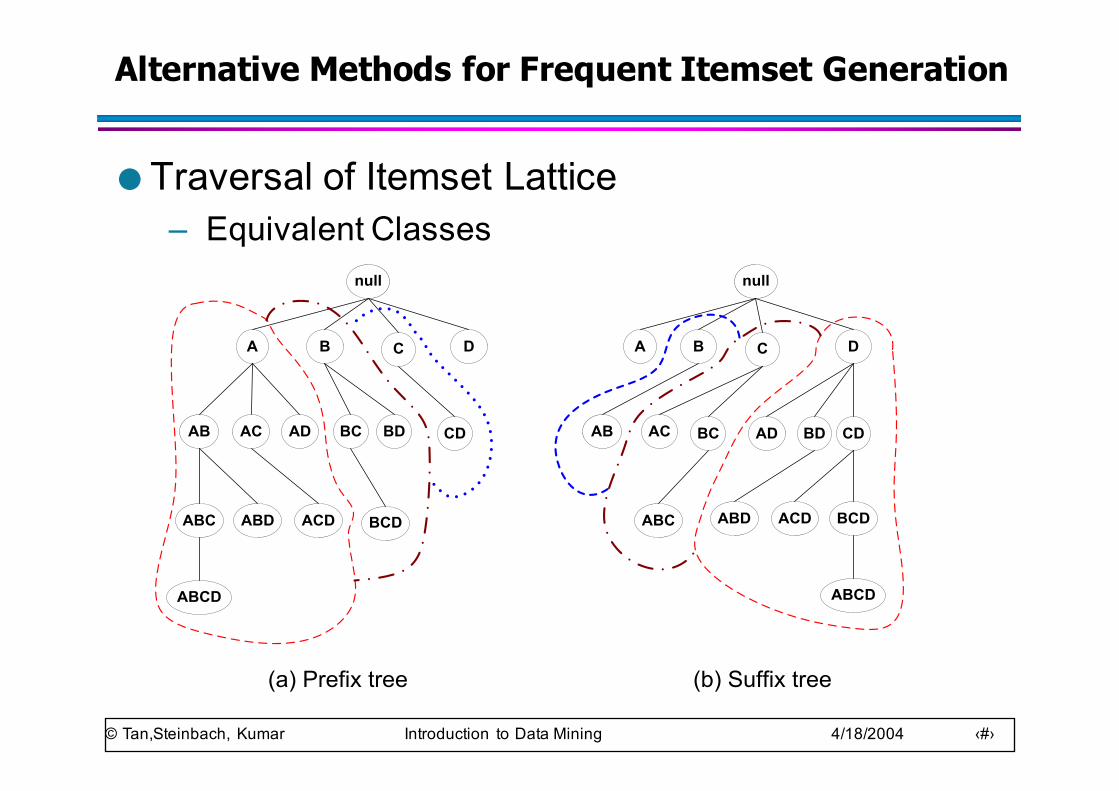
Alternative Methods for Frequent Itemset Generation
● Traversal of Itemset Lattice– Equivalent Classes
null
AB AC AD BC BD CD
A B C D
ABC ABD ACD BCD
ABCD
null
AB AC ADBC BD CD
A B C D
ABC ABD ACD BCD
ABCD
(a) Prefix tree (b) Suffix tree
© Tan,Steinbach, Kumar Introduction to Data Mining 4/18/2004 ‹#›
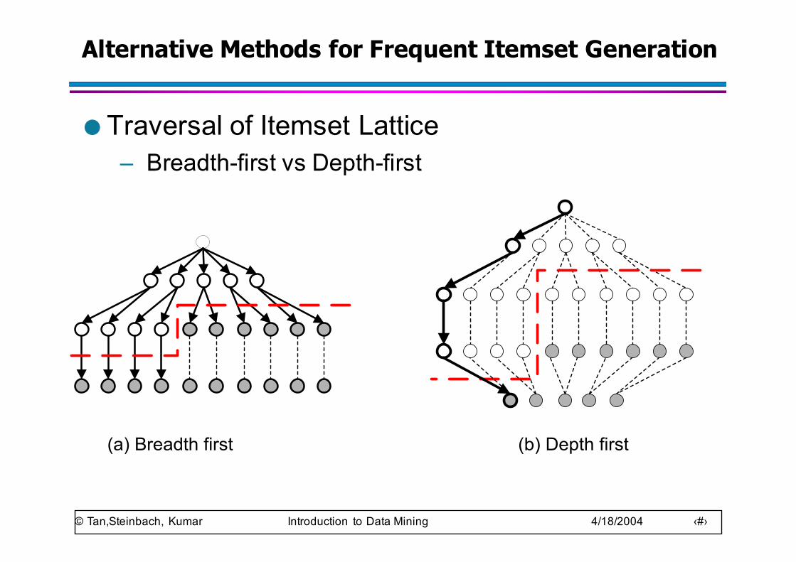
Alternative Methods for Frequent Itemset Generation
● Traversal of Itemset Lattice– Breadth-first vs Depth-first
(a) Breadth first (b) Depth first
© Tan,Steinbach, Kumar Introduction to Data Mining 4/18/2004 ‹#›
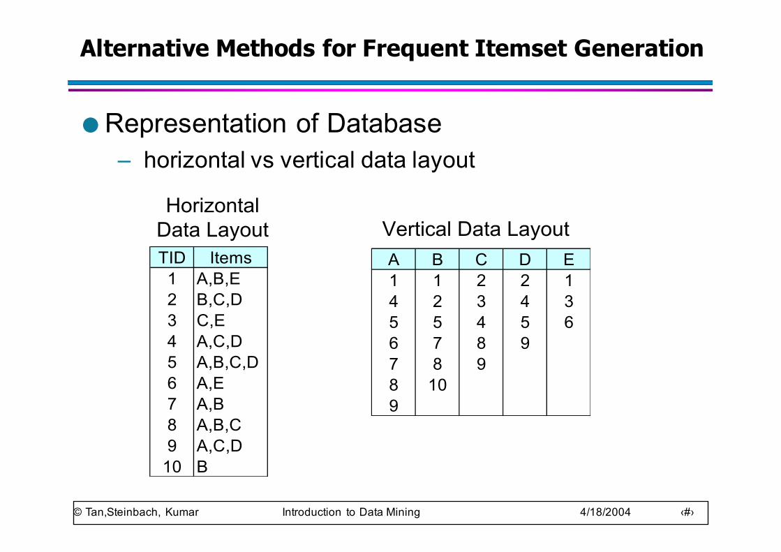
Alternative Methods for Frequent Itemset Generation
● Representation of Database– horizontal vs vertical data layout
TID Items1 A,B,E2 B,C,D3 C,E4 A,C,D5 A,B,C,D6 A,E7 A,B8 A,B,C9 A,C,D10 B
HorizontalData Layout
A B C D E1 1 2 2 14 2 3 4 35 5 4 5 66 7 8 97 8 98 109
Vertical Data Layout
© Tan,Steinbach, Kumar Introduction to Data Mining 4/18/2004 ‹#›
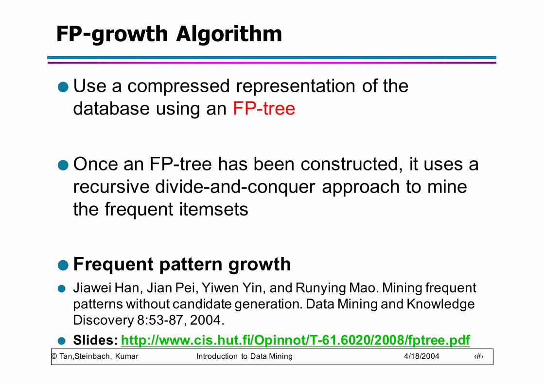
FP-growth Algorithm
● Use a compressed representation of the database using an FP-tree
● Once an FP-tree has been constructed, it uses a recursive divide-and-conquer approach to mine the frequent itemsets
● Frequent pattern growth● Jiawei Han, Jian Pei, Yiwen Yin, and Runying Mao. Mining frequent
patterns without candidate generation. Data Mining and Knowledge Discovery 8:53-87, 2004.
● Slides: http://www.cis.hut.fi/Opinnot/T-61.6020/2008/fptree.pdf

Why FP, not Apriori?
Apriori works well except when:§ Lots of frequent patterns
§ Big set of items§ Low minimum support threshold
§ Long patterns
Why: Candidate sets become huge§ 104 frequent patterns of length 1 → 108 length 2
candidates§ Discovering pattern of length 100 requires at least 2100
candidates (nr of subsets)§ Repeated database scans costly (long patterns)

© Tan,Steinbach, Kumar Introduction to Data Mining 4/18/2004 ‹#›
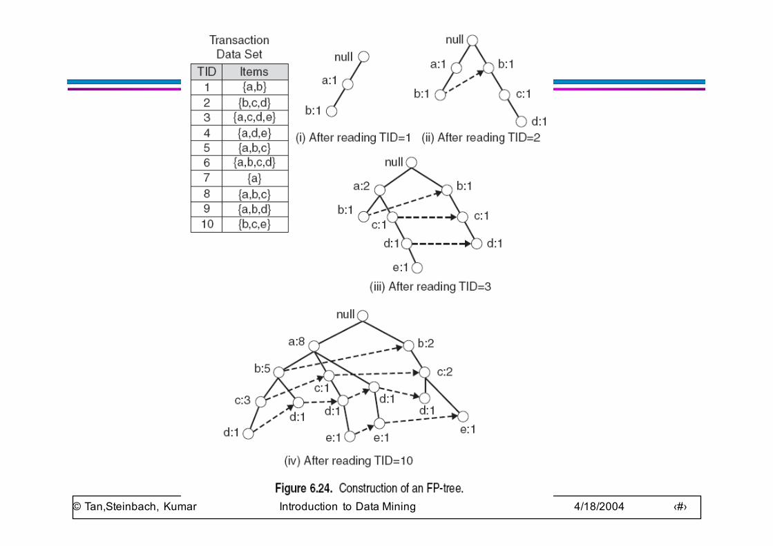
FP-tree construction
TID Items1 {A,B}2 {B,C,D}3 {A,C,D,E}4 {A,D,E}5 {A,B,C}6 {A,B,C,D}7 {B,C}8 {A,B,C}9 {A,B,D}10 {B,C,E}
null
A:1
B:1
null
A:1
B:1
B:1
C:1
D:1
After reading TID=1:
After reading TID=2:
© Tan,Steinbach, Kumar Introduction to Data Mining 4/18/2004 ‹#›
© Tan,Steinbach, Kumar Introduction to Data Mining 4/18/2004 ‹#›
© Tan,Steinbach, Kumar Introduction to Data Mining 4/18/2004 ‹#›
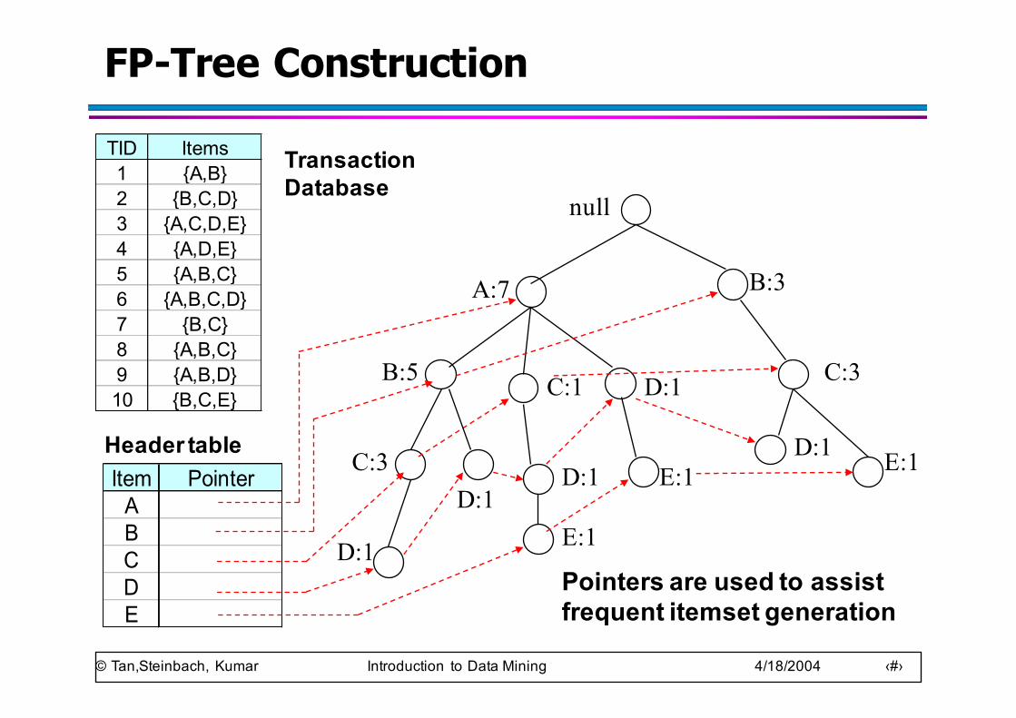
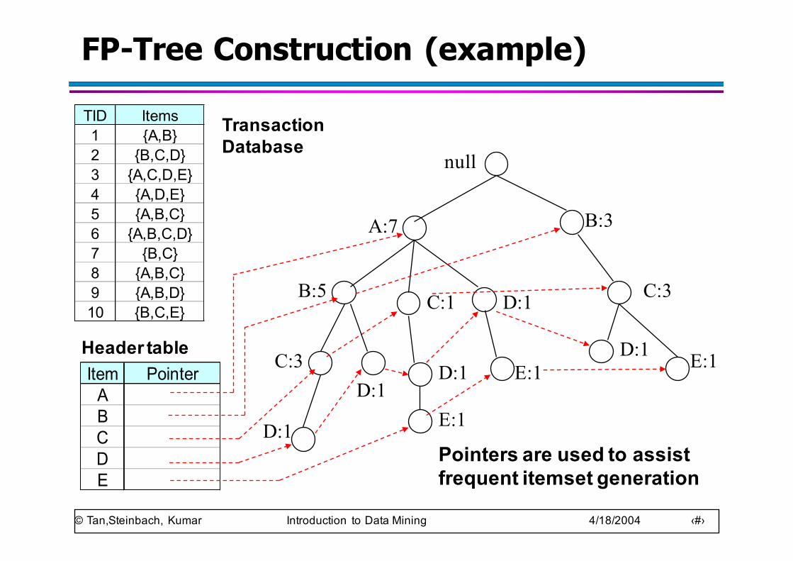
FP-Tree Construction
null
A:7
B:5
B:3
C:3
D:1
C:1
D:1C:3
D:1
D:1
E:1 E:1
TID Items1 {A,B}2 {B,C,D}3 {A,C,D,E}4 {A,D,E}5 {A,B,C}6 {A,B,C,D}7 {B,C}8 {A,B,C}9 {A,B,D}10 {B,C,E}
Pointers are used to assist frequent itemset generation
D:1E:1
Transaction Database
Item PointerABCDE
Header table
© Tan,Steinbach, Kumar Introduction to Data Mining 4/18/2004 ‹#›
© Tan,Steinbach, Kumar Introduction to Data Mining 4/18/2004 ‹#›
© Tan,Steinbach, Kumar Introduction to Data Mining 4/18/2004 ‹#›
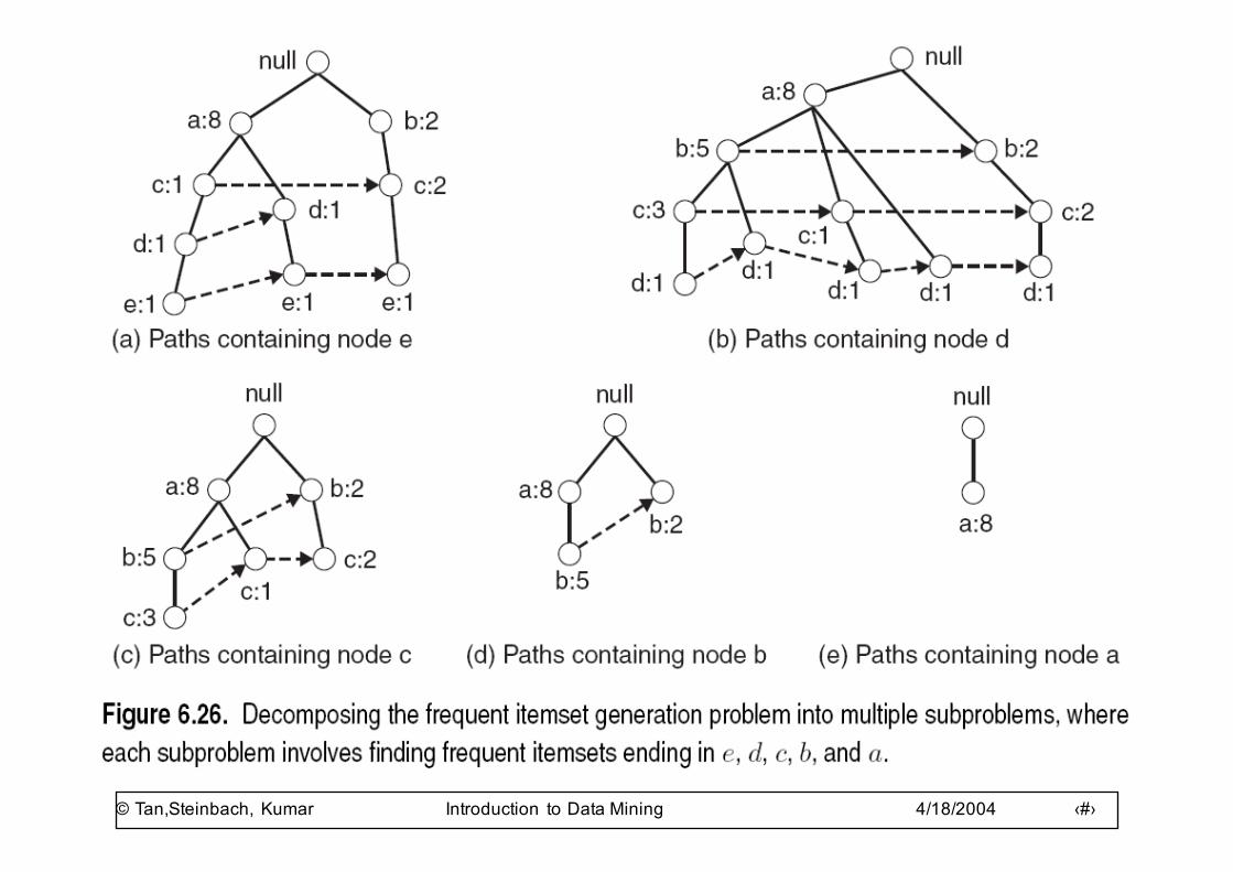
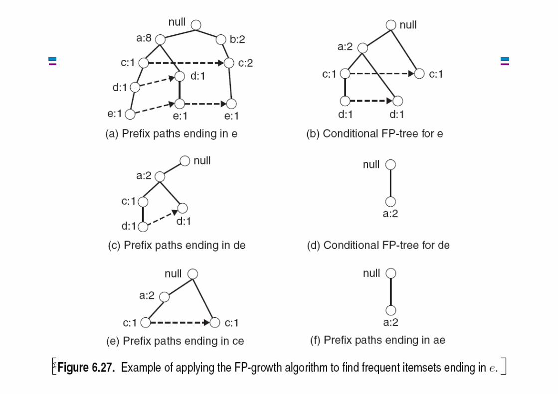
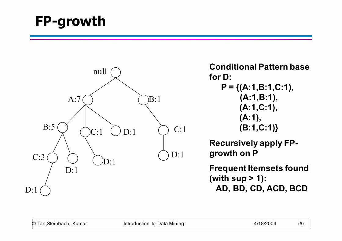
FP-growth
null
A:7
B:5
B:1
C:1
D:1
C:1
D:1C:3
D:1
D:1
Conditional Pattern base for D:
P = {(A:1,B:1,C:1),(A:1,B:1), (A:1,C:1),(A:1), (B:1,C:1)}
Recursively apply FP-growth on PFrequent Itemsets found (with sup > 1):
AD, BD, CD, ACD, BCD
D:1
© Tan,Steinbach, Kumar Introduction to Data Mining 4/18/2004 ‹#›
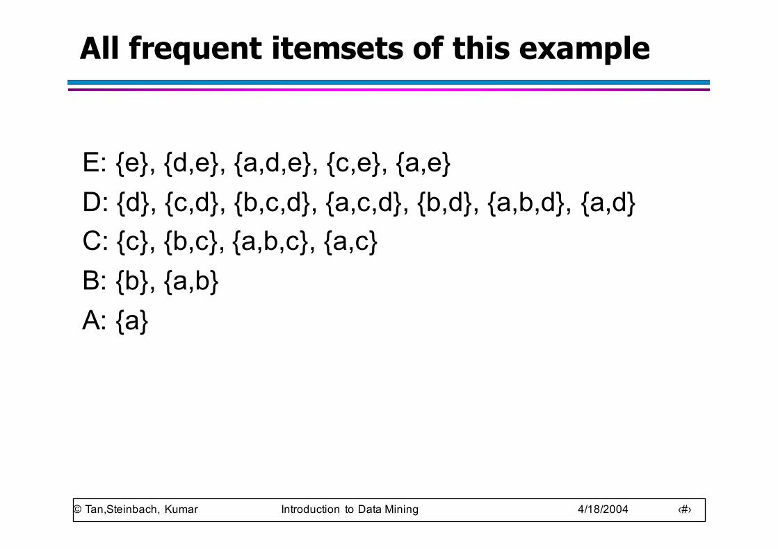
All frequent itemsets of this example
E: {e}, {d,e}, {a,d,e}, {c,e}, {a,e}D: {d}, {c,d}, {b,c,d}, {a,c,d}, {b,d}, {a,b,d}, {a,d}C: {c}, {b,c}, {a,b,c}, {a,c}B: {b}, {a,b}A: {a}
© Tan,Steinbach, Kumar Introduction to Data Mining 4/18/2004 ‹#›
FP-Tree Construction (example)
null
A:7
B:5
B:3
C:3
D:1
C:1
D:1C:3
D:1
D:1
E:1 E:1
TID Items1 {A,B}2 {B,C,D}3 {A,C,D,E}4 {A,D,E}5 {A,B,C}6 {A,B,C,D}7 {B,C}8 {A,B,C}9 {A,B,D}10 {B,C,E}
Pointers are used to assist frequent itemset generation
D:1E:1
Transaction Database
Item PointerABCDE
Header table
© Tan,Steinbach, Kumar Introduction to Data Mining 4/18/2004 ‹#›
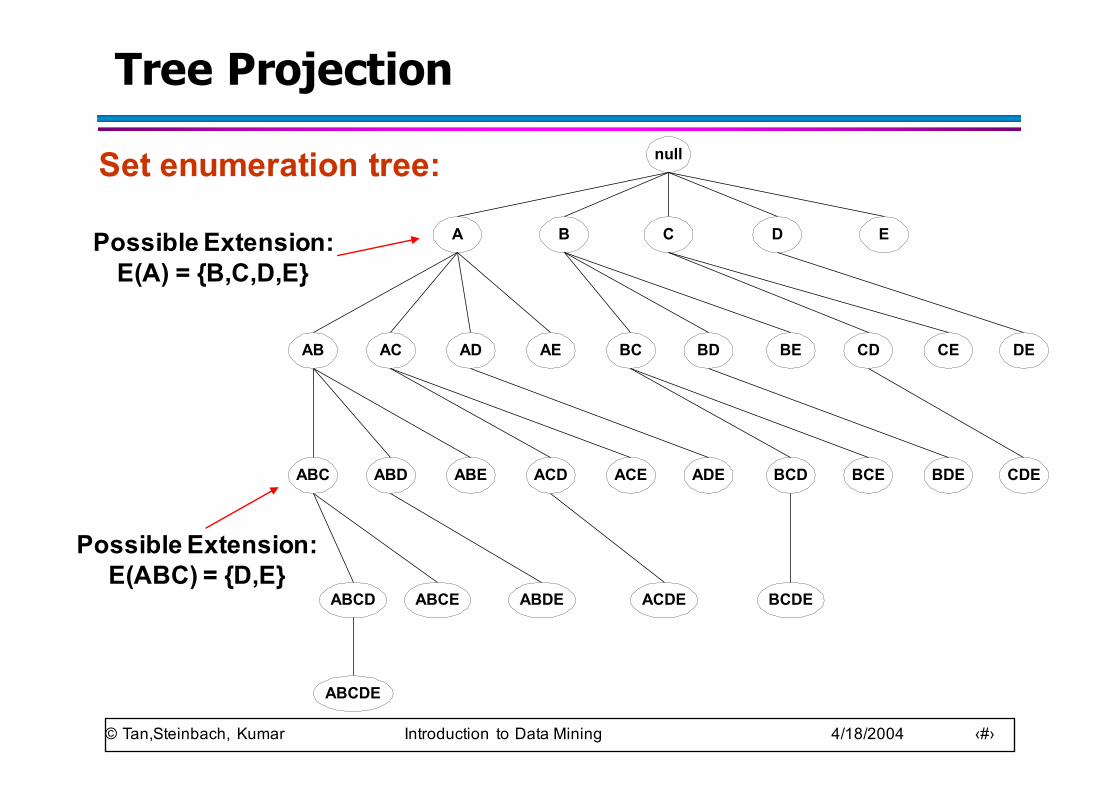
Tree Projection
Set enumeration tree: null
AB AC AD AE BC BD BE CD CE DE
A B C D E
ABC ABD ABE ACD ACE ADE BCD BCE BDE CDE
ABCD ABCE ABDE ACDE BCDE
ABCDE
Possible Extension: E(A) = {B,C,D,E}
Possible Extension: E(ABC) = {D,E}
© Tan,Steinbach, Kumar Introduction to Data Mining 4/18/2004 ‹#›
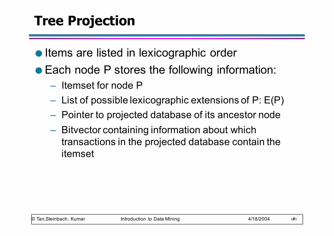
Tree Projection
● Items are listed in lexicographic order● Each node P stores the following information:
– Itemset for node P– List of possible lexicographic extensions of P: E(P)– Pointer to projected database of its ancestor node– Bitvector containing information about which
transactions in the projected database contain the itemset
© Tan,Steinbach, Kumar Introduction to Data Mining 4/18/2004 ‹#›
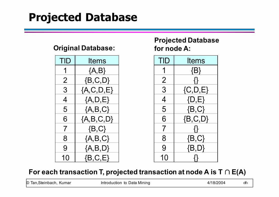
Projected Database
TID Items1 {A,B}2 {B,C,D}3 {A,C,D,E}4 {A,D,E}5 {A,B,C}6 {A,B,C,D}7 {B,C}8 {A,B,C}9 {A,B,D}10 {B,C,E}
TID Items1 {B}2 {}3 {C,D,E}4 {D,E}5 {B,C}6 {B,C,D}7 {}8 {B,C}9 {B,D}10 {}
Original Database:Projected Database for node A:
For each transaction T, projected transaction at node A is T ∩ E(A)
© Tan,Steinbach, Kumar Introduction to Data Mining 4/18/2004 ‹#›
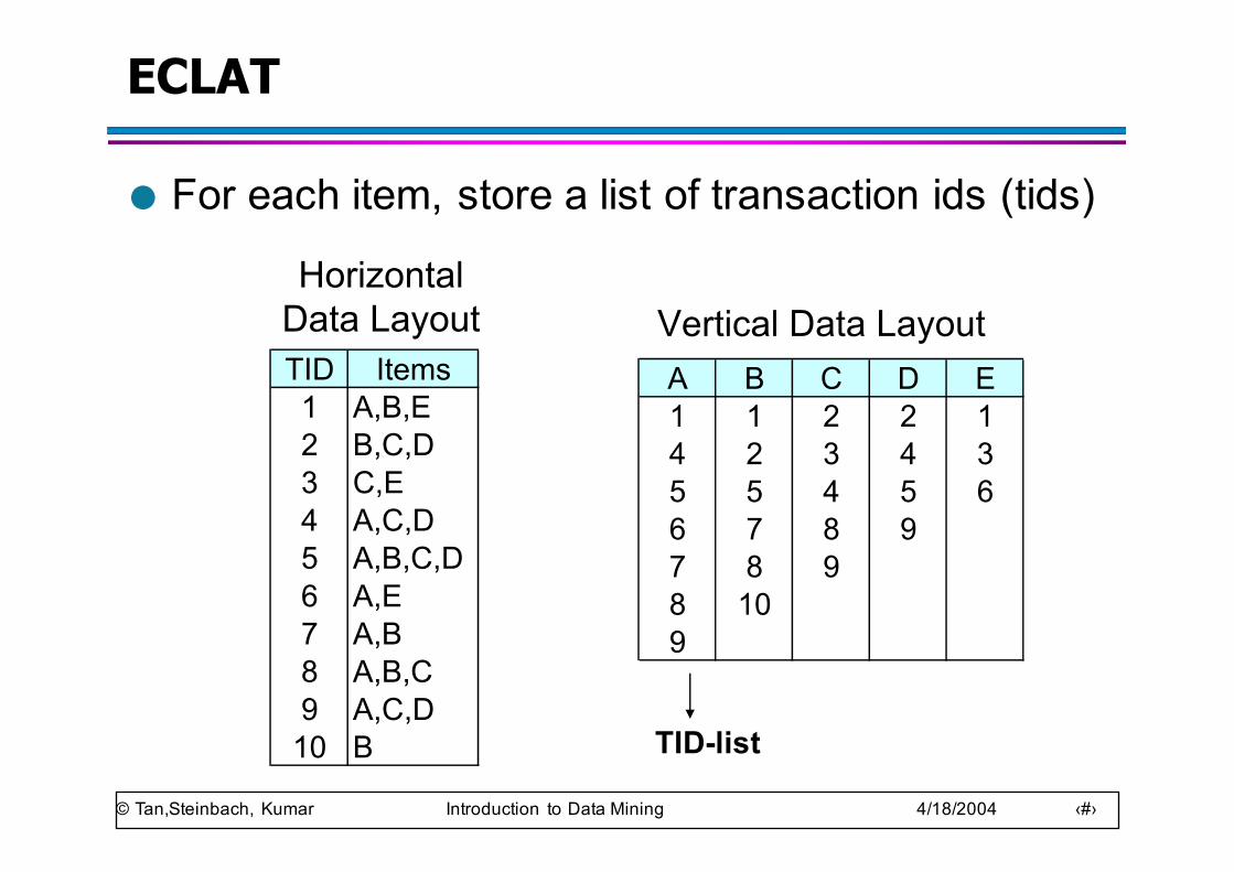
ECLAT
● For each item, store a list of transaction ids (tids)
TID Items1 A,B,E2 B,C,D3 C,E4 A,C,D5 A,B,C,D6 A,E7 A,B8 A,B,C9 A,C,D
10 B
HorizontalData Layout
A B C D E1 1 2 2 14 2 3 4 35 5 4 5 66 7 8 97 8 98 109
Vertical Data Layout
TID-list
© Tan,Steinbach, Kumar Introduction to Data Mining 4/18/2004 ‹#›
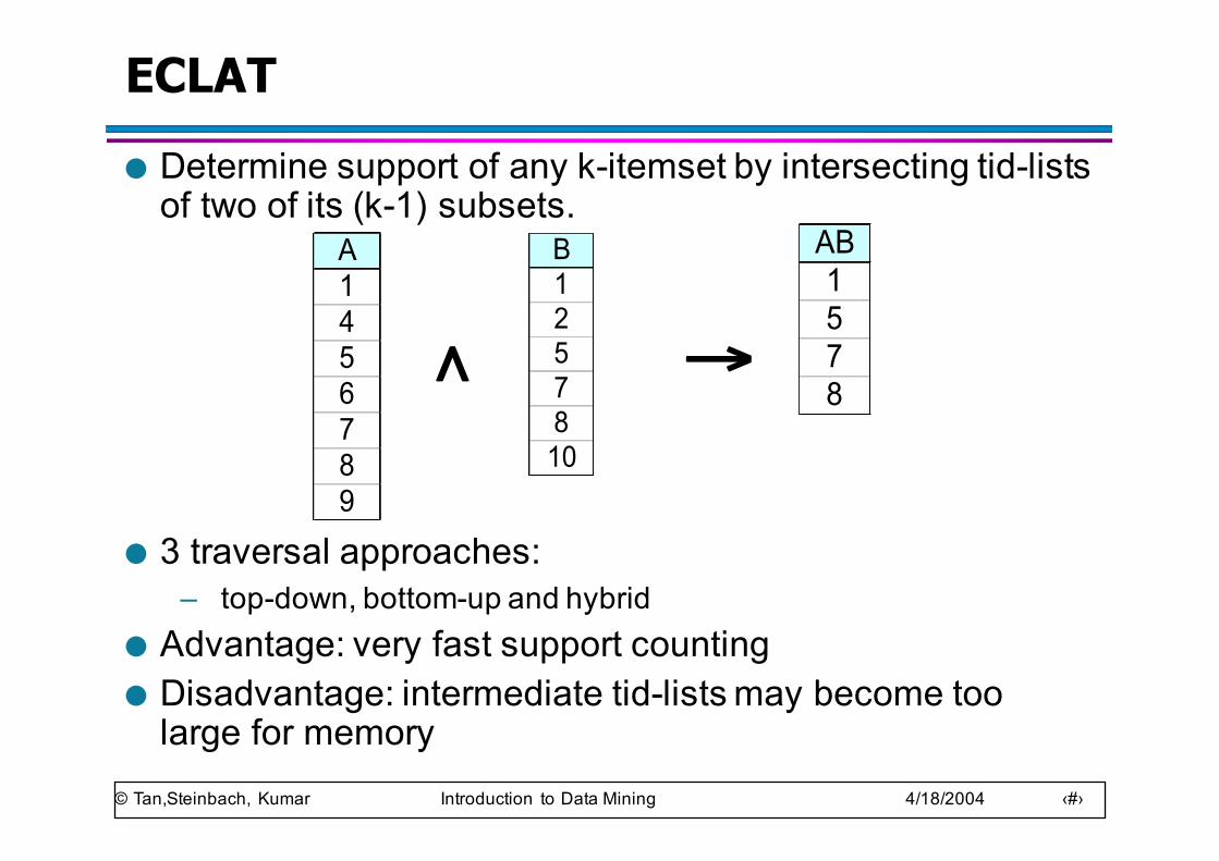
ECLAT● Determine support of any k-itemset by intersecting tid-lists
of two of its (k-1) subsets.
● 3 traversal approaches: – top-down, bottom-up and hybrid
● Advantage: very fast support counting● Disadvantage: intermediate tid-lists may become too
large for memory
A1456789
B1257810
∧ →
AB1578
© Tan,Steinbach, Kumar Introduction to Data Mining 4/18/2004 ‹#›
Rule Generation
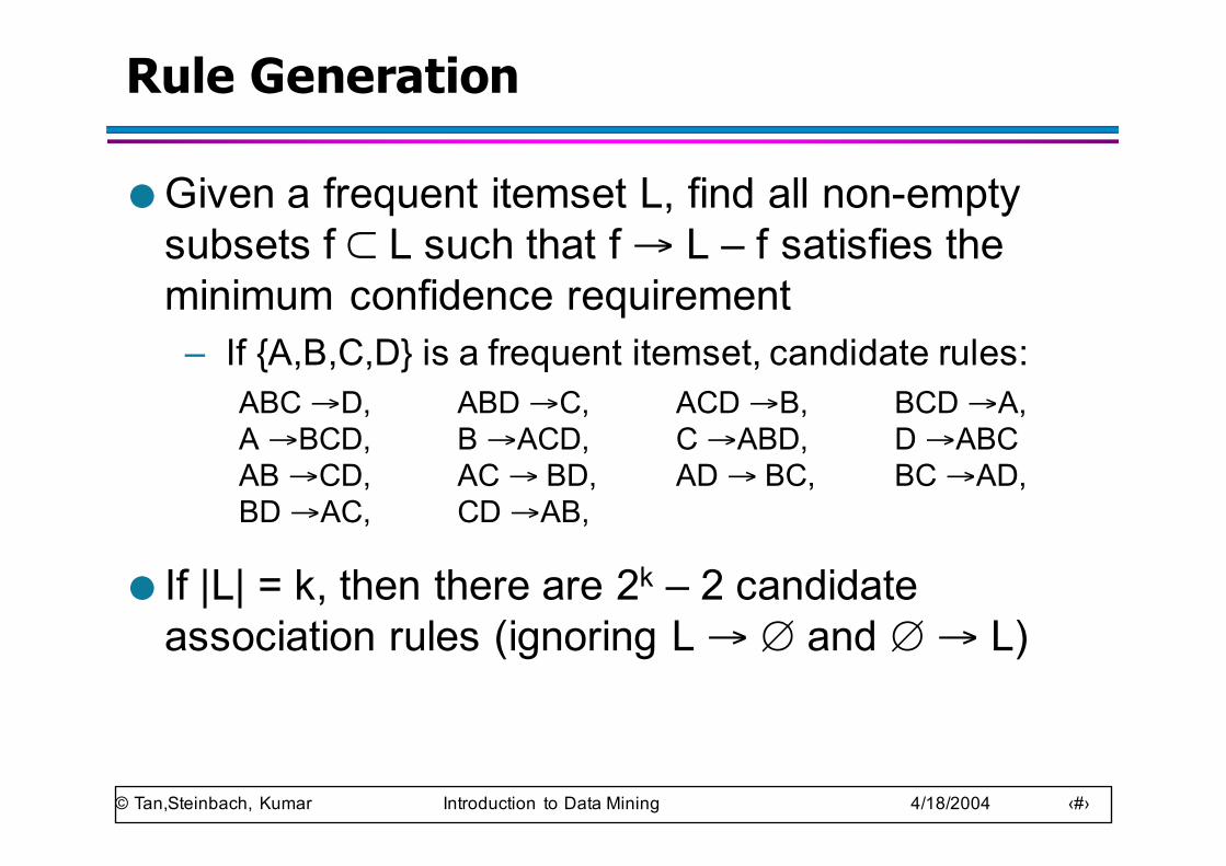
● Given a frequent itemset L, find all non-empty subsets f ⊂ L such that f → L – f satisfies the minimum confidence requirement
– If {A,B,C,D} is a frequent itemset, candidate rules:ABC →D, ABD →C, ACD →B, BCD →A, A →BCD, B →ACD, C →ABD, D →ABCAB →CD, AC → BD, AD → BC, BC →AD, BD →AC, CD →AB,
● If |L| = k, then there are 2k – 2 candidate association rules (ignoring L → ∅ and ∅ → L)
© Tan,Steinbach, Kumar Introduction to Data Mining 4/18/2004 ‹#›
Rule Generation
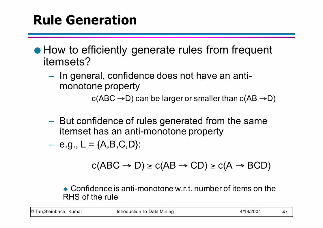
● How to efficiently generate rules from frequent itemsets?
– In general, confidence does not have an anti-monotone property
c(ABC →D) can be larger or smaller than c(AB →D)
– But confidence of rules generated from the same itemset has an anti-monotone property
– e.g., L = {A,B,C,D}:
c(ABC → D) ≥ c(AB → CD) ≥ c(A → BCD)
u Confidence is anti-monotone w.r.t. number of items on the RHS of the rule
© Tan,Steinbach, Kumar Introduction to Data Mining 4/18/2004 ‹#›
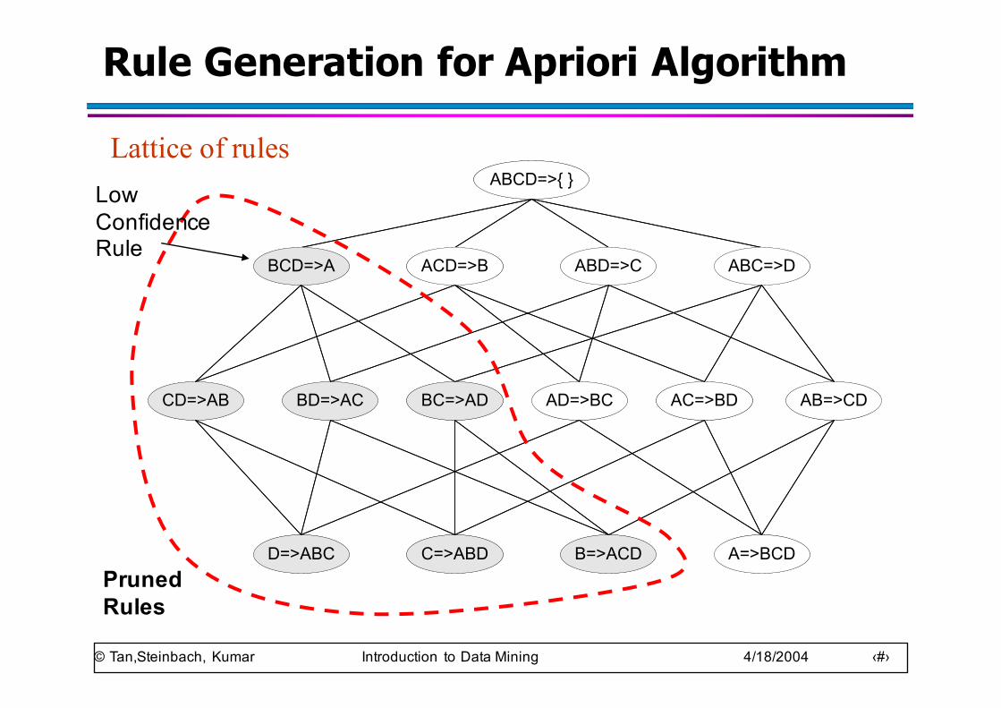
Rule Generation for Apriori Algorithm
ABCD=>{ }
BCD=>A ACD=>B ABD=>C ABC=>D
BC=>ADBD=>ACCD=>AB AD=>BC AC=>BD AB=>CD
D=>ABC C=>ABD B=>ACD A=>BCD
Lattice of rulesABCD=>{ }
BCD=>A ACD=>B ABD=>C ABC=>D
BC=>ADBD=>ACCD=>AB AD=>BC AC=>BD AB=>CD
D=>ABC C=>ABD B=>ACD A=>BCDPruned Rules
Low Confidence Rule
© Tan,Steinbach, Kumar Introduction to Data Mining 4/18/2004 ‹#›
Rule Generation for Apriori Algorithm
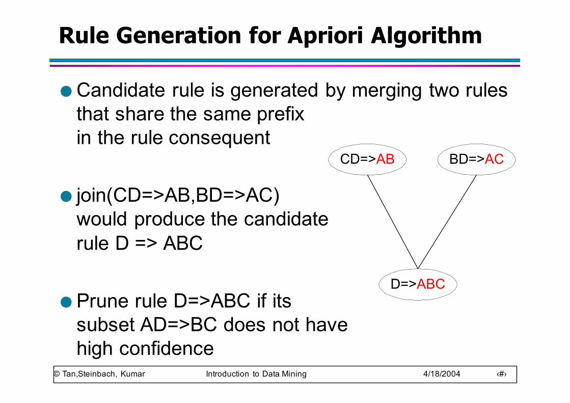
● Candidate rule is generated by merging two rules that share the same prefixin the rule consequent
● join(CD=>AB,BD=>AC)would produce the candidaterule D => ABC
● Prune rule D=>ABC if itssubset AD=>BC does not havehigh confidence
BD=>ACCD=>AB
D=>ABC
© Tan,Steinbach, Kumar Introduction to Data Mining 4/18/2004 ‹#›
Effect of Support Distribution
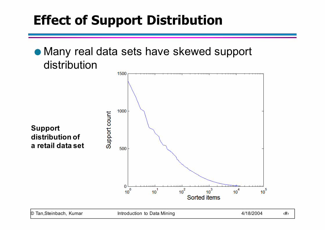
● Many real data sets have skewed support distribution
Support distribution of a retail data set
© Tan,Steinbach, Kumar Introduction to Data Mining 4/18/2004 ‹#›
Effect of Support Distribution
● How to set the appropriate minsup threshold?– If minsup is set too high, we could miss itemsets
involving interesting rare items (e.g., expensive products)
– If minsup is set too low, it is computationally expensive and the number of itemsets is very large
● Using a single minimum support threshold may not be effective
© Tan,Steinbach, Kumar Introduction to Data Mining 4/18/2004 ‹#›
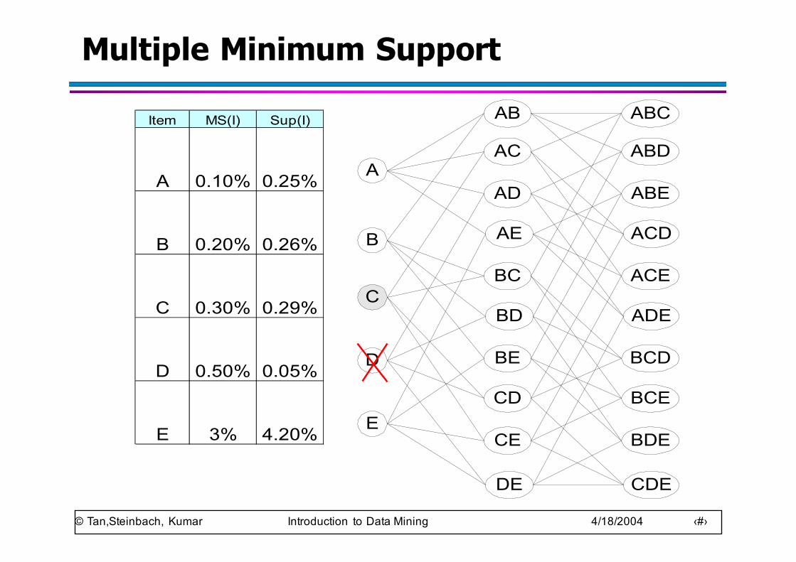
Multiple Minimum Support
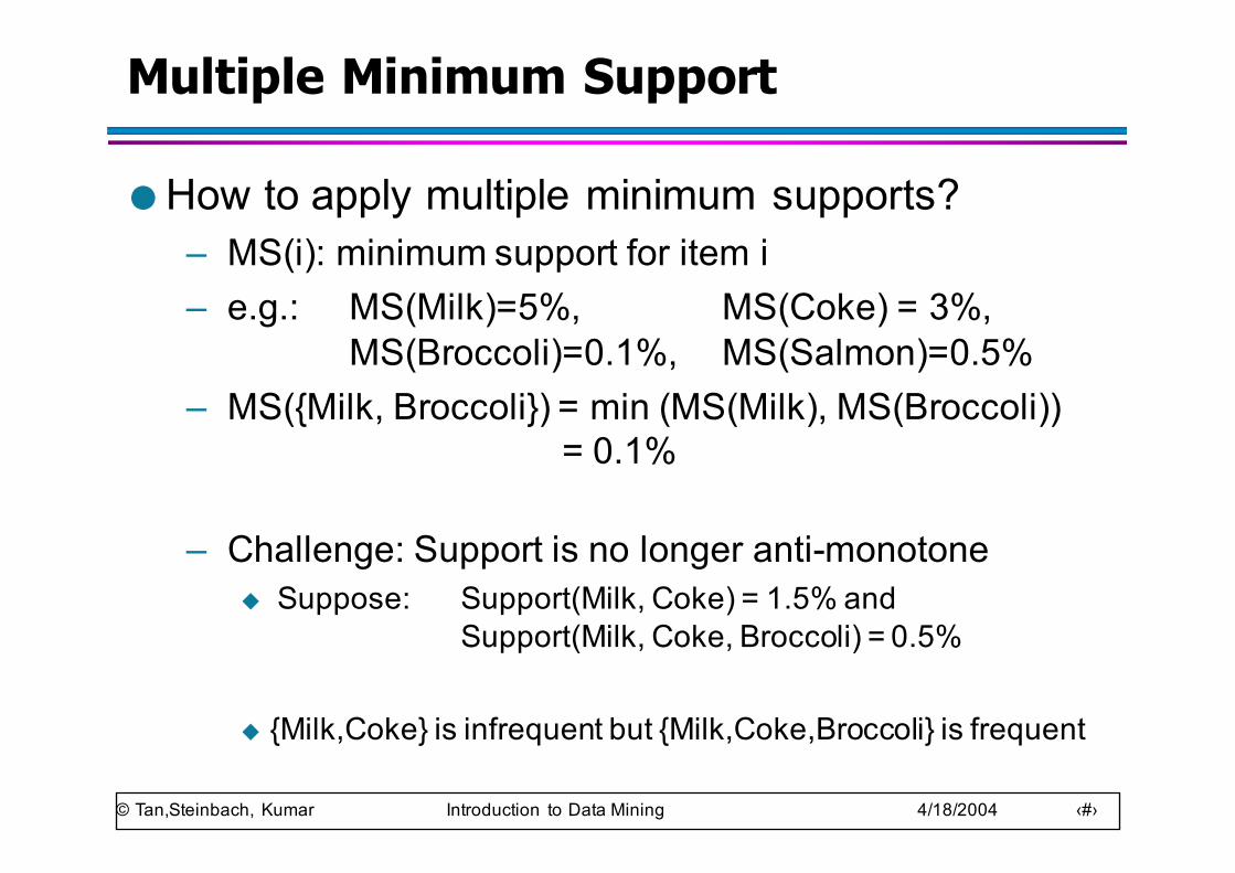
● How to apply multiple minimum supports?– MS(i): minimum support for item i– e.g.: MS(Milk)=5%, MS(Coke) = 3%,
MS(Broccoli)=0.1%, MS(Salmon)=0.5%– MS({Milk, Broccoli}) = min (MS(Milk), MS(Broccoli))
= 0.1%
– Challenge: Support is no longer anti-monotoneu Suppose: Support(Milk, Coke) = 1.5% and
Support(Milk, Coke, Broccoli) = 0.5%
u {Milk,Coke} is infrequent but {Milk,Coke,Broccoli} is frequent
© Tan,Steinbach, Kumar Introduction to Data Mining 4/18/2004 ‹#›
Multiple Minimum Support
A
Item MS(I) Sup(I)
A 0.10% 0.25%
B 0.20% 0.26%
C 0.30% 0.29%
D 0.50% 0.05%
E 3% 4.20%
B
C
D
E
AB
AC
AD
AE
BC
BD
BE
CD
CE
DE
ABC
ABD
ABE
ACD
ACE
ADE
BCD
BCE
BDE
CDE
© Tan,Steinbach, Kumar Introduction to Data Mining 4/18/2004 ‹#›
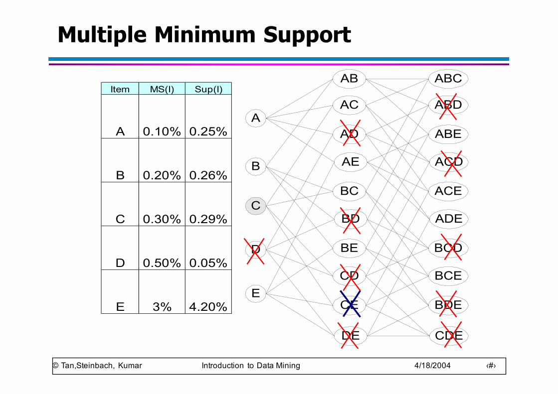
Multiple Minimum Support
A
B
C
D
E
AB
AC
AD
AE
BC
BD
BE
CD
CE
DE
ABC
ABD
ABE
ACD
ACE
ADE
BCD
BCE
BDE
CDE
Item MS(I) Sup(I)
A 0.10% 0.25%
B 0.20% 0.26%
C 0.30% 0.29%
D 0.50% 0.05%
E 3% 4.20%
© Tan,Steinbach, Kumar Introduction to Data Mining 4/18/2004 ‹#›
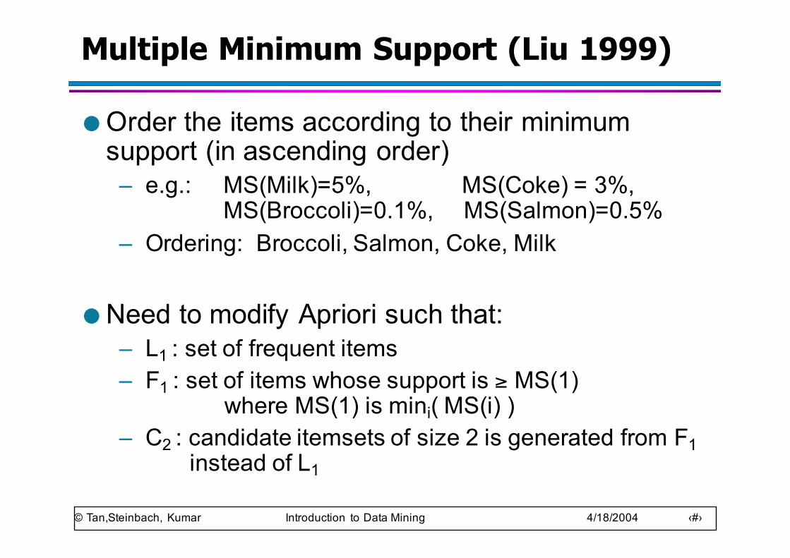
Multiple Minimum Support (Liu 1999)
● Order the items according to their minimum support (in ascending order)
– e.g.: MS(Milk)=5%, MS(Coke) = 3%,MS(Broccoli)=0.1%, MS(Salmon)=0.5%
– Ordering: Broccoli, Salmon, Coke, Milk
● Need to modify Apriori such that:– L1 : set of frequent items– F1 : set of items whose support is ≥ MS(1)
where MS(1) is mini( MS(i) )– C2 : candidate itemsets of size 2 is generated from F1
instead of L1
© Tan,Steinbach, Kumar Introduction to Data Mining 4/18/2004 ‹#›
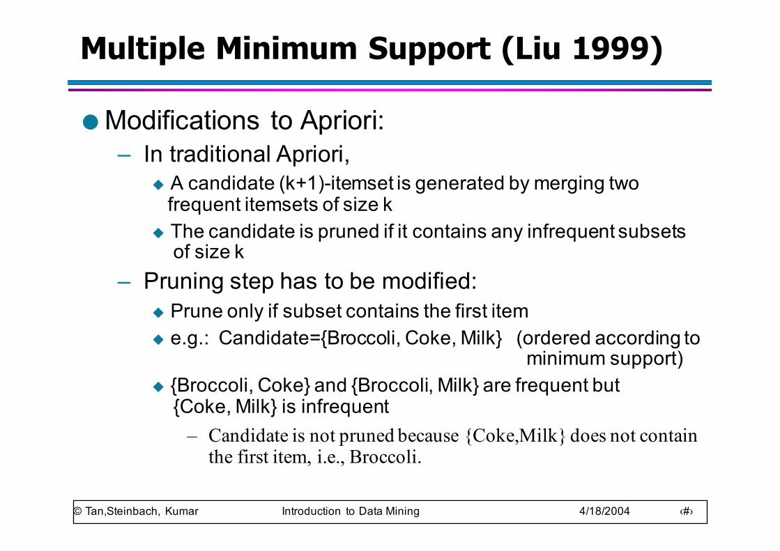
Multiple Minimum Support (Liu 1999)
● Modifications to Apriori:– In traditional Apriori,
u A candidate (k+1)-itemset is generated by merging twofrequent itemsets of size k
u The candidate is pruned if it contains any infrequent subsetsof size k
– Pruning step has to be modified:u Prune only if subset contains the first itemu e.g.: Candidate={Broccoli, Coke, Milk} (ordered according to
minimum support)u {Broccoli, Coke} and {Broccoli, Milk} are frequent but
{Coke, Milk} is infrequent– Candidate is not pruned because {Coke,Milk} does not contain
the first item, i.e., Broccoli.
© Tan,Steinbach, Kumar Introduction to Data Mining 4/18/2004 ‹#›
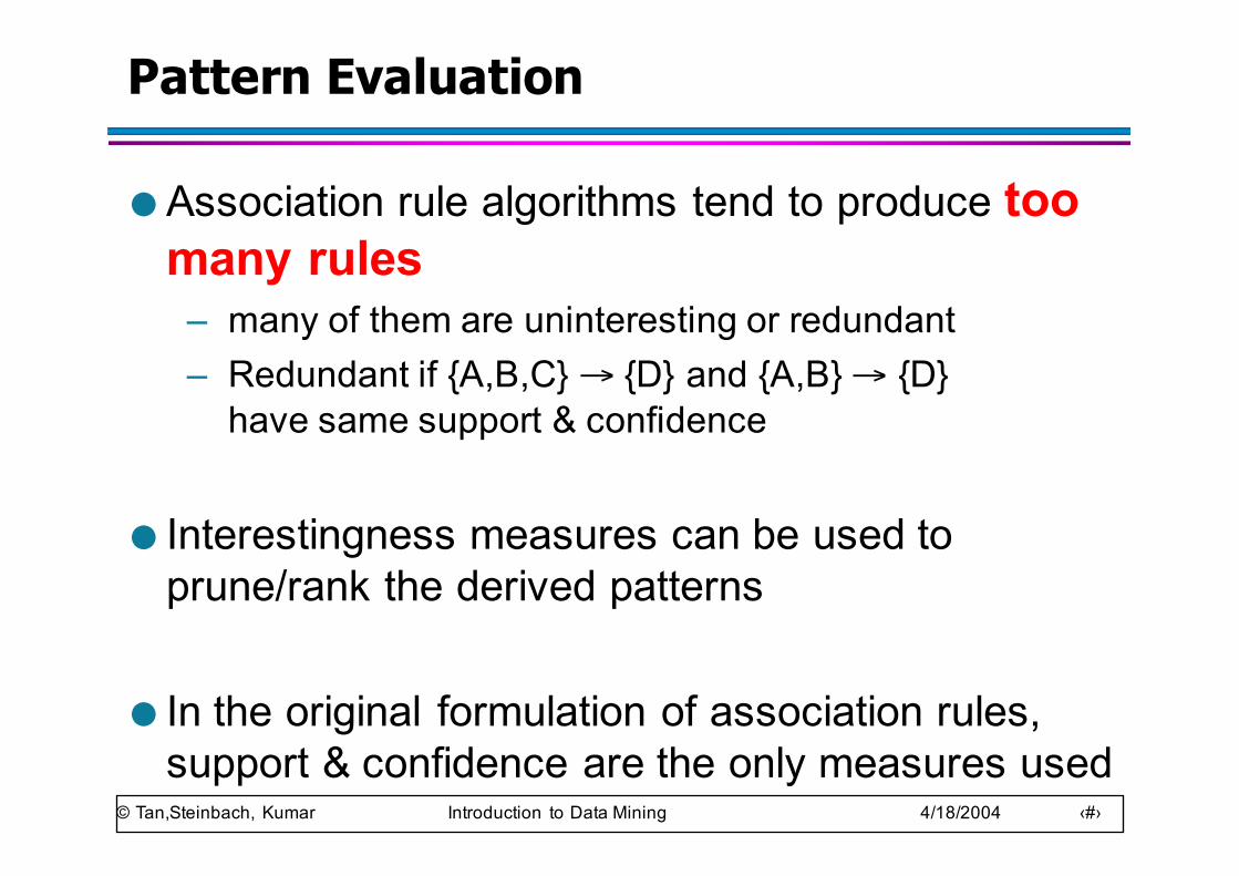
Pattern Evaluation
● Association rule algorithms tend to produce too many rules
– many of them are uninteresting or redundant– Redundant if {A,B,C} → {D} and {A,B} → {D}
have same support & confidence
● Interestingness measures can be used to prune/rank the derived patterns
● In the original formulation of association rules, support & confidence are the only measures used
© Tan,Steinbach, Kumar Introduction to Data Mining 4/18/2004 ‹#›
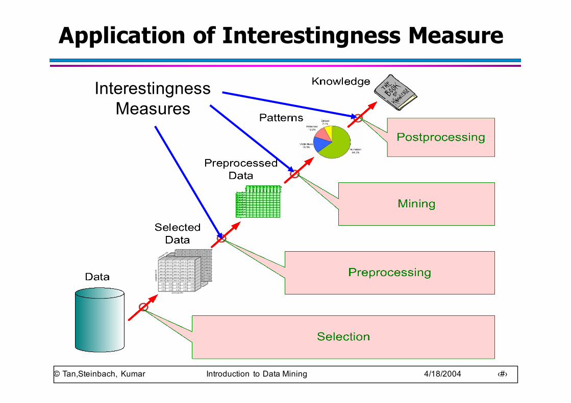
Application of Interestingness Measure
Interestingness Measures
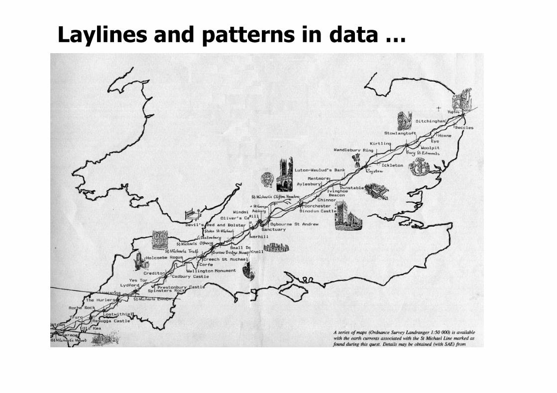
Laylines and patterns in data …
© Tan,Steinbach, Kumar Introduction to Data Mining 4/18/2004 ‹#›
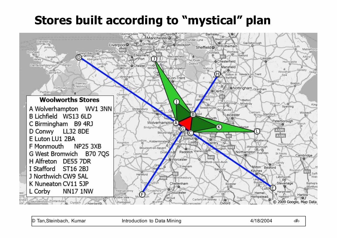
Stores built according to “mystical” plan
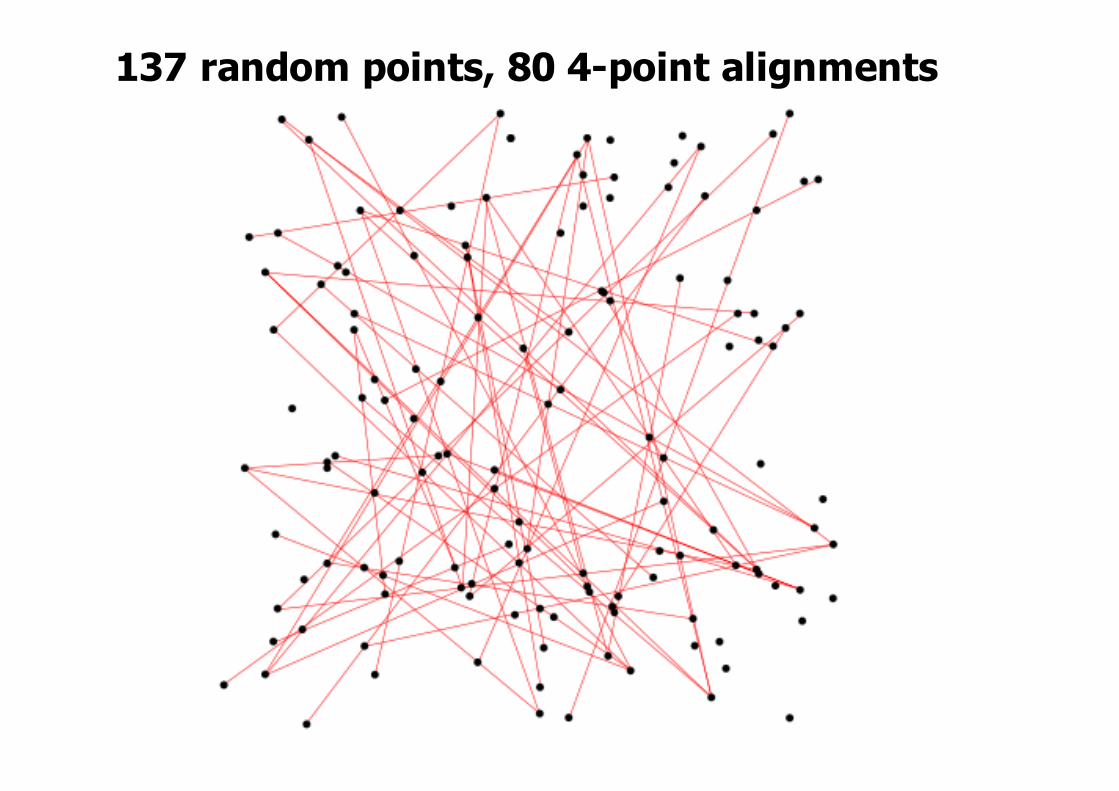
137 random points, 80 4-point alignments
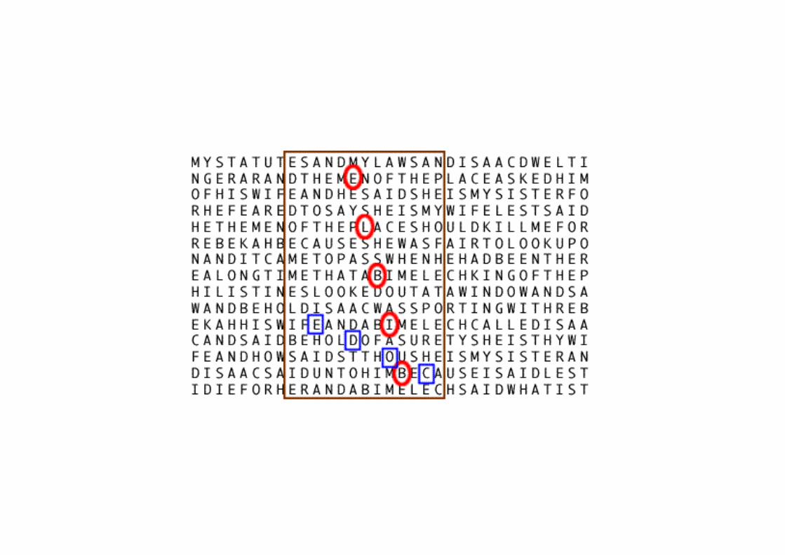
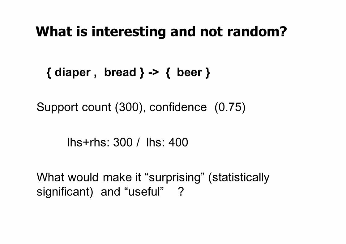
What is interesting and not random?
{ diaper , bread } -> { beer }
Support count (300), confidence (0.75)
lhs+rhs: 300 / lhs: 400
What would make it “surprising” (statistically significant) and “useful” ?
© Tan,Steinbach, Kumar Introduction to Data Mining 4/18/2004 ‹#›
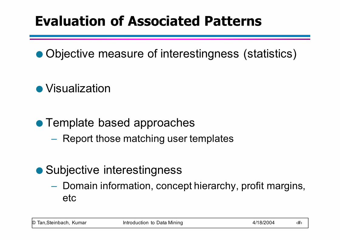
Evaluation of Associated Patterns
● Objective measure of interestingness (statistics)
● Visualization
● Template based approaches– Report those matching user templates
● Subjective interestingness– Domain information, concept hierarchy, profit margins,
etc
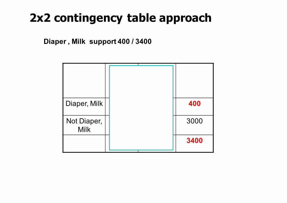
2x2 contingency table approach
Beer Not Beer
Diaper, Milk 300 100 400
Not Diaper, Milk
1000 2000 3000
1300 2100 3400
Diaper , Milk support 400 / 3400
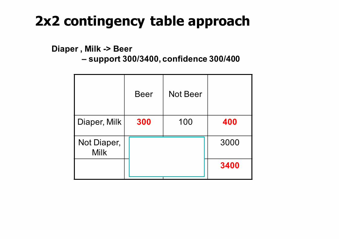
2x2 contingency table approach
Beer Not Beer
Diaper, Milk 300 100 400
Not Diaper, Milk
1000 2000 3000
1300 2100 3400
Diaper , Milk -> Beer – support 300/3400, confidence 300/400
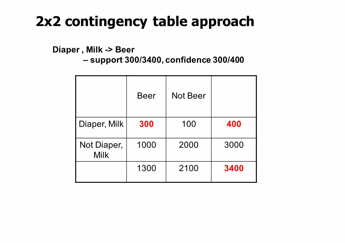
2x2 contingency table approach
Beer Not Beer
Diaper, Milk 300 100 400
Not Diaper, Milk
1000 2000 3000
1300 2100 3400
Diaper , Milk -> Beer – support 300/3400, confidence 300/400
© Tan,Steinbach, Kumar Introduction to Data Mining 4/18/2004 ‹#›
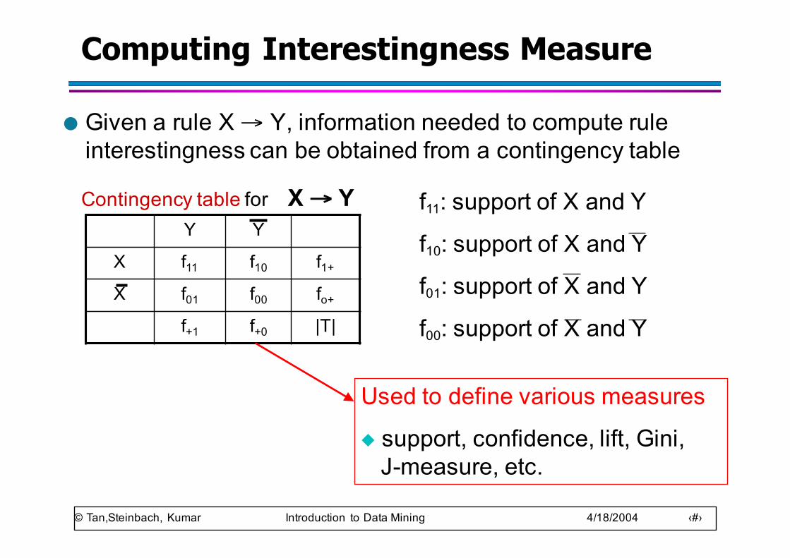
Computing Interestingness Measure
● Given a rule X → Y, information needed to compute rule interestingness can be obtained from a contingency table
Y Y
X f11 f10 f1+
X f01 f00 fo+
f+1 f+0 |T|
Contingency table for X → Y f11: support of X and Y
f10: support of X and Y
f01: support of X and Y
f00: support of X and Y
Used to define various measures
◆ support, confidence, lift, Gini,J-measure, etc.
© Tan,Steinbach, Kumar Introduction to Data Mining 4/18/2004 ‹#›
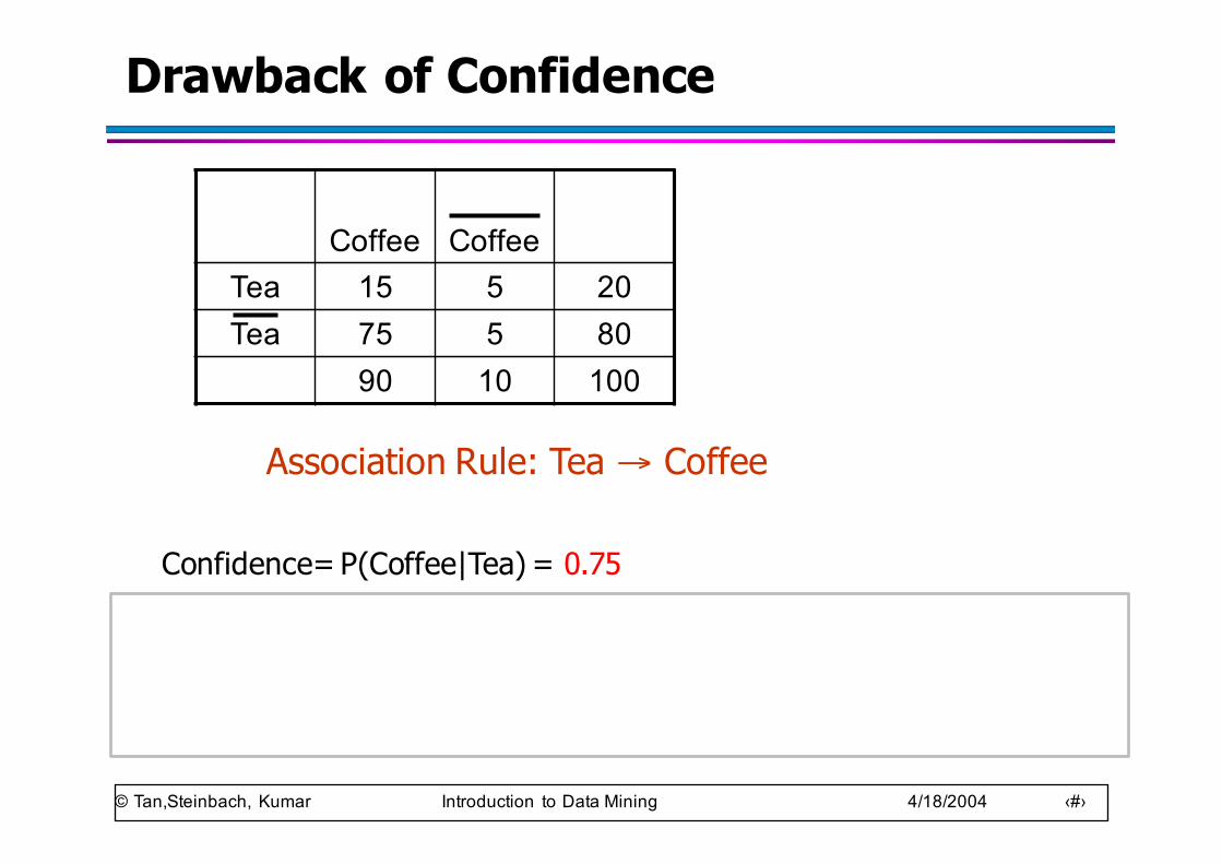
Drawback of Confidence
Coffee CoffeeTea 15 5 20Tea 75 5 80
90 10 100
Association Rule: Tea → Coffee
Confidence= P(Coffee|Tea) = 0.75but P(Coffee) = 0.9⇒ Although confidence is high, rule is misleading⇒ P(Coffee|Tea) = 0.9375
© Tan,Steinbach, Kumar Introduction to Data Mining 4/18/2004 ‹#›
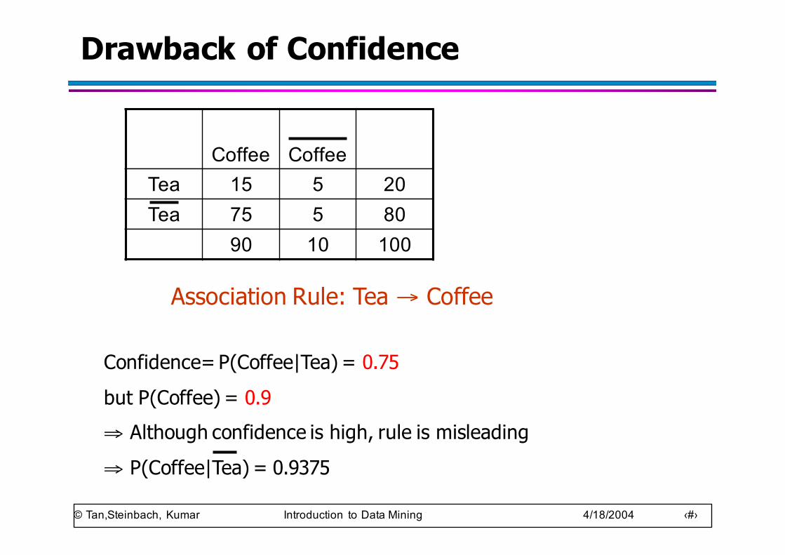
Drawback of Confidence
Coffee CoffeeTea 15 5 20Tea 75 5 80
90 10 100
Association Rule: Tea → Coffee
Confidence= P(Coffee|Tea) = 0.75but P(Coffee) = 0.9⇒ Although confidence is high, rule is misleading⇒ P(Coffee|Tea) = 0.9375
© Tan,Steinbach, Kumar Introduction to Data Mining 4/18/2004 ‹#›
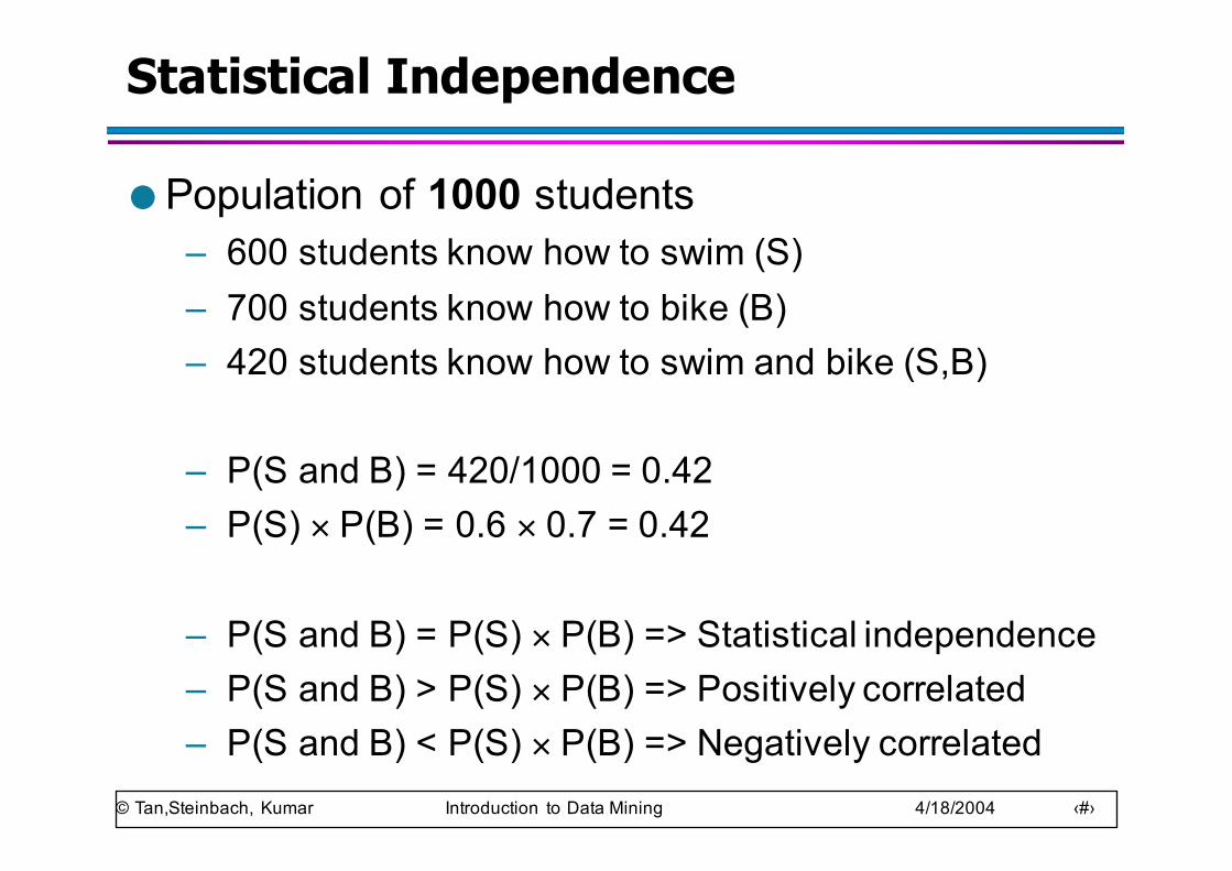
Statistical Independence
● Population of 1000 students– 600 students know how to swim (S)– 700 students know how to bike (B)– 420 students know how to swim and bike (S,B)
– P(S and B) = 420/1000 = 0.42– P(S) × P(B) = 0.6 × 0.7 = 0.42
– P(S and B) = P(S) × P(B) => Statistical independence– P(S and B) > P(S) × P(B) => Positively correlated– P(S and B) < P(S) × P(B) => Negatively correlated
© Tan,Steinbach, Kumar Introduction to Data Mining 4/18/2004 ‹#›
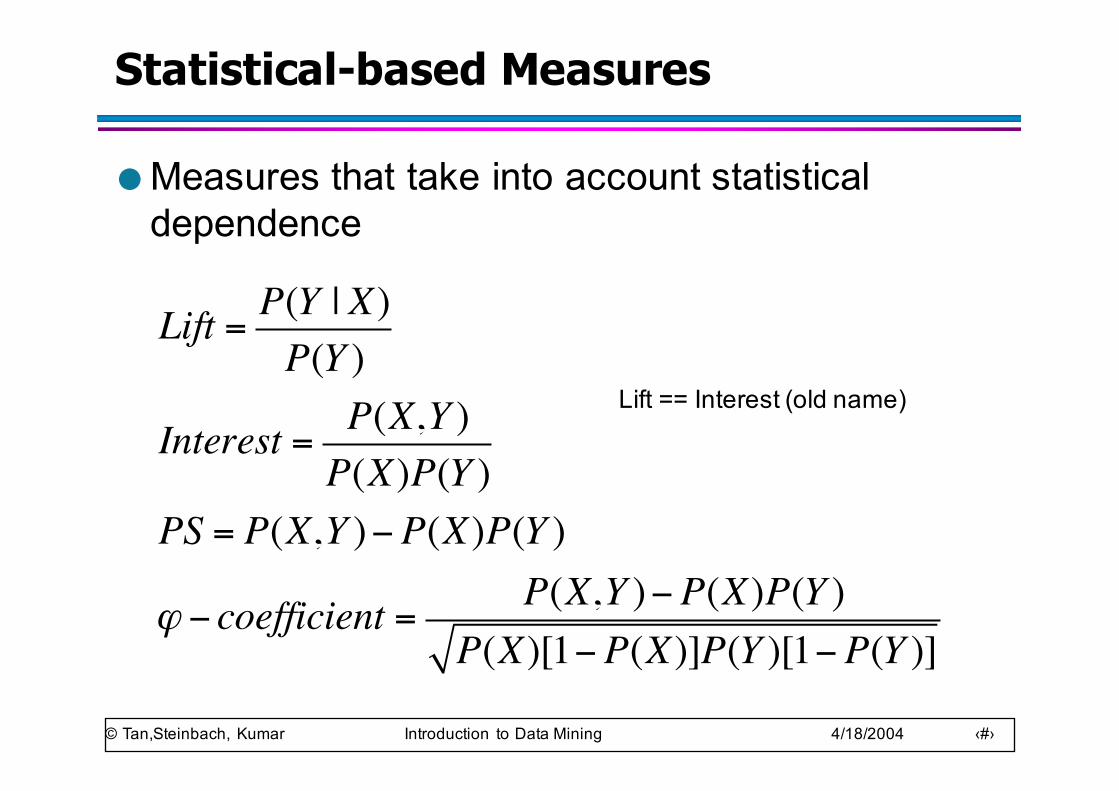
Statistical-based Measures
● Measures that take into account statistical dependence
Lift = P(Y | X)P(Y )
Interest = P(X,Y )P(X)P(Y )
PS = P(X,Y )−P(X)P(Y )
ϕ − coefficient = P(X,Y )−P(X)P(Y )P(X)[1−P(X)]P(Y )[1−P(Y )]
Lift == Interest (old name)
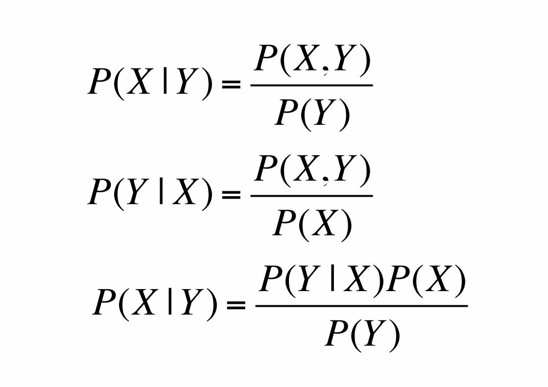
P(X |Y ) = P(X,Y )P(Y )
P(Y | X) = P(X,Y )P(X)
P(X |Y ) = P(Y | X)P(X)P(Y )
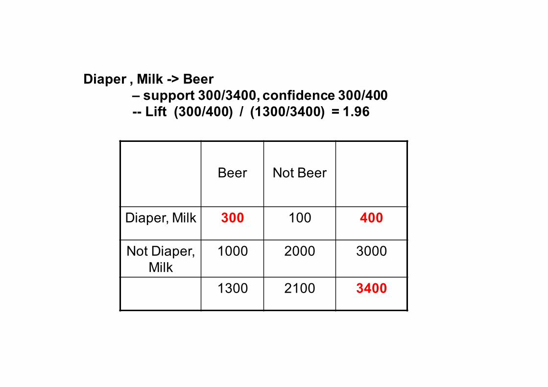
Beer Not Beer
Diaper, Milk 300 100 400
Not Diaper, Milk
1000 2000 3000
1300 2100 3400
Diaper , Milk -> Beer – support 300/3400, confidence 300/400-- Lift (300/400) / (1300/3400) = 1.96
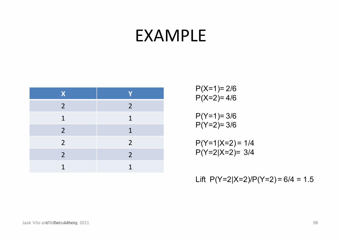
EXAMPLE
X Y2 21 12 12 22 21 1
JaakViloandotherauthorsUT:DataMining2011 98
P(X=1)= 2/6P(X=2)= 4/6
P(Y=1)= 3/6P(Y=2)= 3/6
P(Y=1|X=2) = 1/4P(Y=2|X=2)= 3/4
Lift P(Y=2|X=2)/P(Y=2) = 6/4 = 1.5
© Tan,Steinbach, Kumar Introduction to Data Mining 4/18/2004 ‹#›
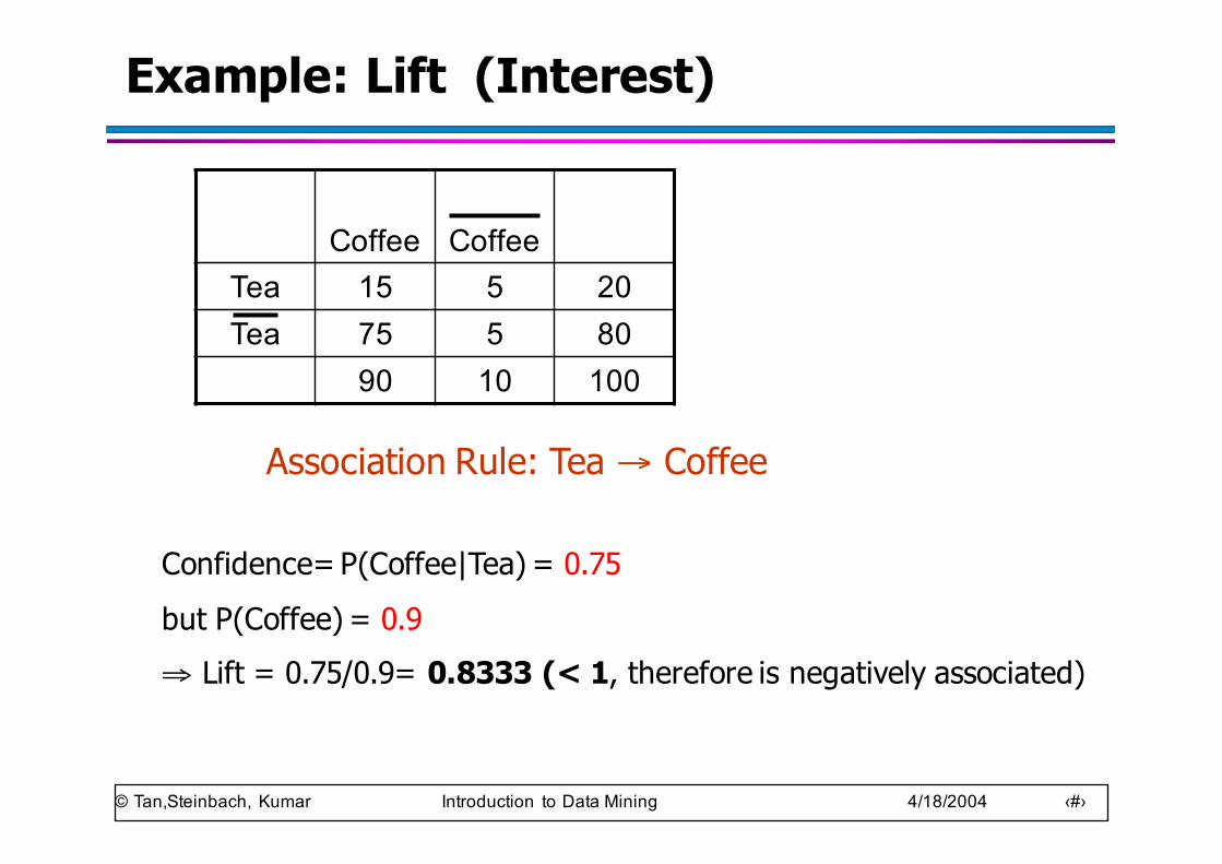
Example: Lift (Interest)
Coffee CoffeeTea 15 5 20Tea 75 5 80
90 10 100
Association Rule: Tea → Coffee
Confidence= P(Coffee|Tea) = 0.75but P(Coffee) = 0.9⇒ Lift = 0.75/0.9= 0.8333 (< 1, therefore is negatively associated)
© Tan,Steinbach, Kumar Introduction to Data Mining 4/18/2004 ‹#›
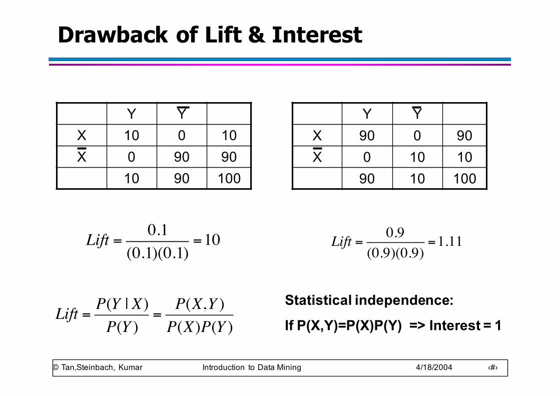
Drawback of Lift & Interest
Y YX 10 0 10X 0 90 90
10 90 100
Y YX 90 0 90X 0 10 10
90 10 100
Lift = 0.1(0.1)(0.1)
=10 Lift = 0.9(0.9)(0.9)
=1.11
Statistical independence:
If P(X,Y)=P(X)P(Y) => Interest = 1Lift = P(Y | X)
P(Y )=
P(X,Y )P(X)P(Y )
101
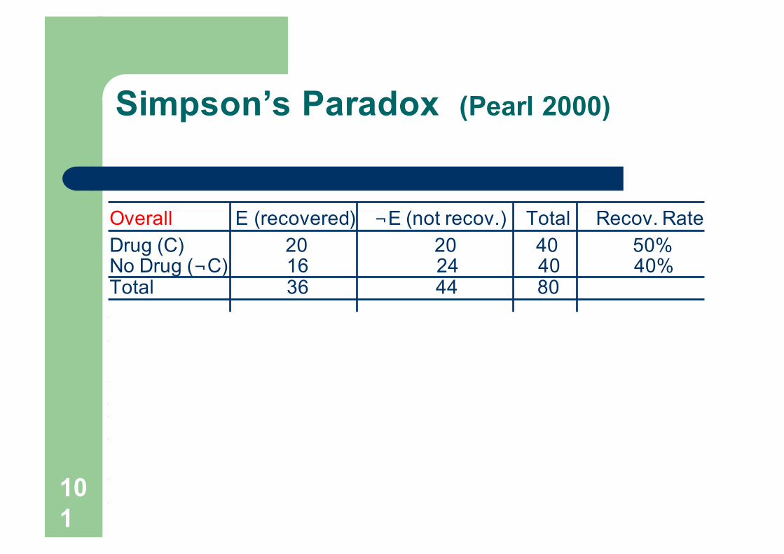
Simpson’s Paradox (Pearl 2000)
Overall E (recovered) ¬E (not recov.) Total Recov. RateDrug (C) 20 20 40 50% No Drug (¬C) 16 24 40 40%Total 36 44 80
Males E (recovered) ¬E (not recov.) Total Recov. RateDrug (C) 18 12 30 60%No Drug (¬C) 7 3 10 70%Total 25 15 40
Females E (recovered) ¬E (not recov.) Total Recov. RateDrug (C) 2 8 10 20%No Drug (¬C) 9 21 30 30%Total 11 29 40
102
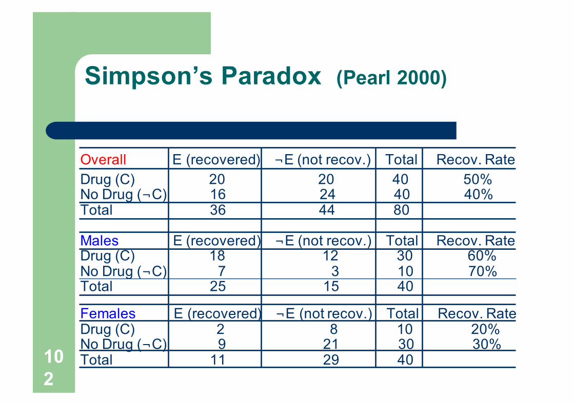
Simpson’s Paradox (Pearl 2000)
Overall E (recovered) ¬E (not recov.) Total Recov. RateDrug (C) 20 20 40 50% No Drug (¬C) 16 24 40 40%Total 36 44 80
Males E (recovered) ¬E (not recov.) Total Recov. RateDrug (C) 18 12 30 60%No Drug (¬C) 7 3 10 70%Total 25 15 40
Females E (recovered) ¬E (not recov.) Total Recov. RateDrug (C) 2 8 10 20%No Drug (¬C) 9 21 30 30%Total 11 29 40
Confounding factors
l There may be some other hidden factors
l Stratified data may show different results
l Statistics …
103
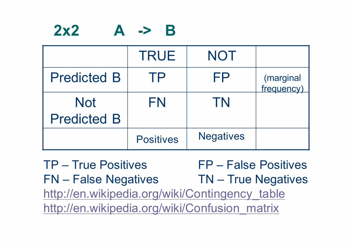
2x2 A -> B
104
TRUE NOT Predicted B TP FP (marginal
frequency)Not
Predicted BFN TN
Positives Negatives
TP – True Positives FP – False PositivesFN – False Negatives TN – True Negativeshttp://en.wikipedia.org/wiki/Contingency_tablehttp://en.wikipedia.org/wiki/Confusion_matrix
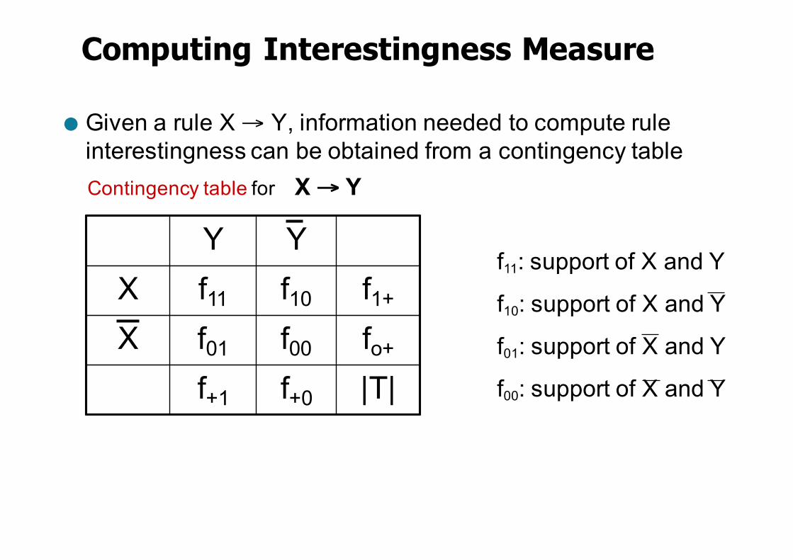
Computing Interestingness Measure
● Given a rule X → Y, information needed to compute rule interestingness can be obtained from a contingency table
Y Y X f11 f10 f1+
X f01 f00 fo+
f+1 f+0 |T|
Contingency table for X → Y
f11: support of X and Y
f10: support of X and Y
f01: support of X and Y
f00: support of X and Y
© Tan,Steinbach, Kumar Introduction to Data Mining 4/18/2004 ‹#›
© Tan,Steinbach, Kumar Introduction to Data Mining 4/18/2004 ‹#›
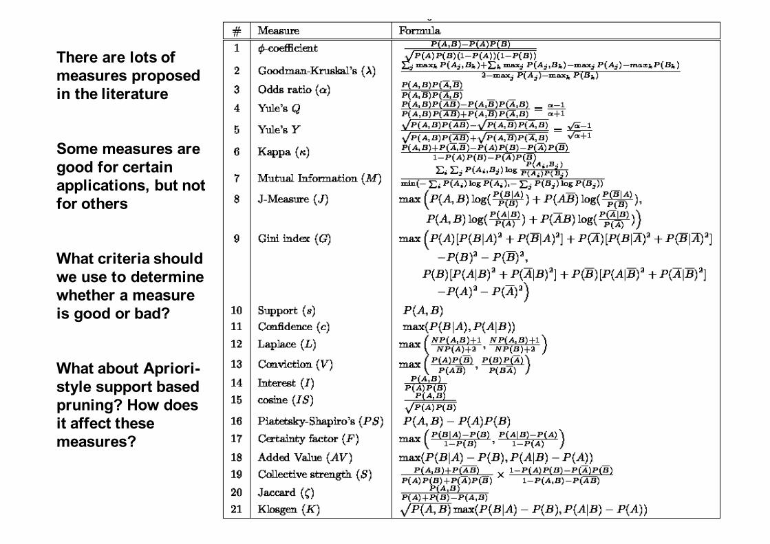
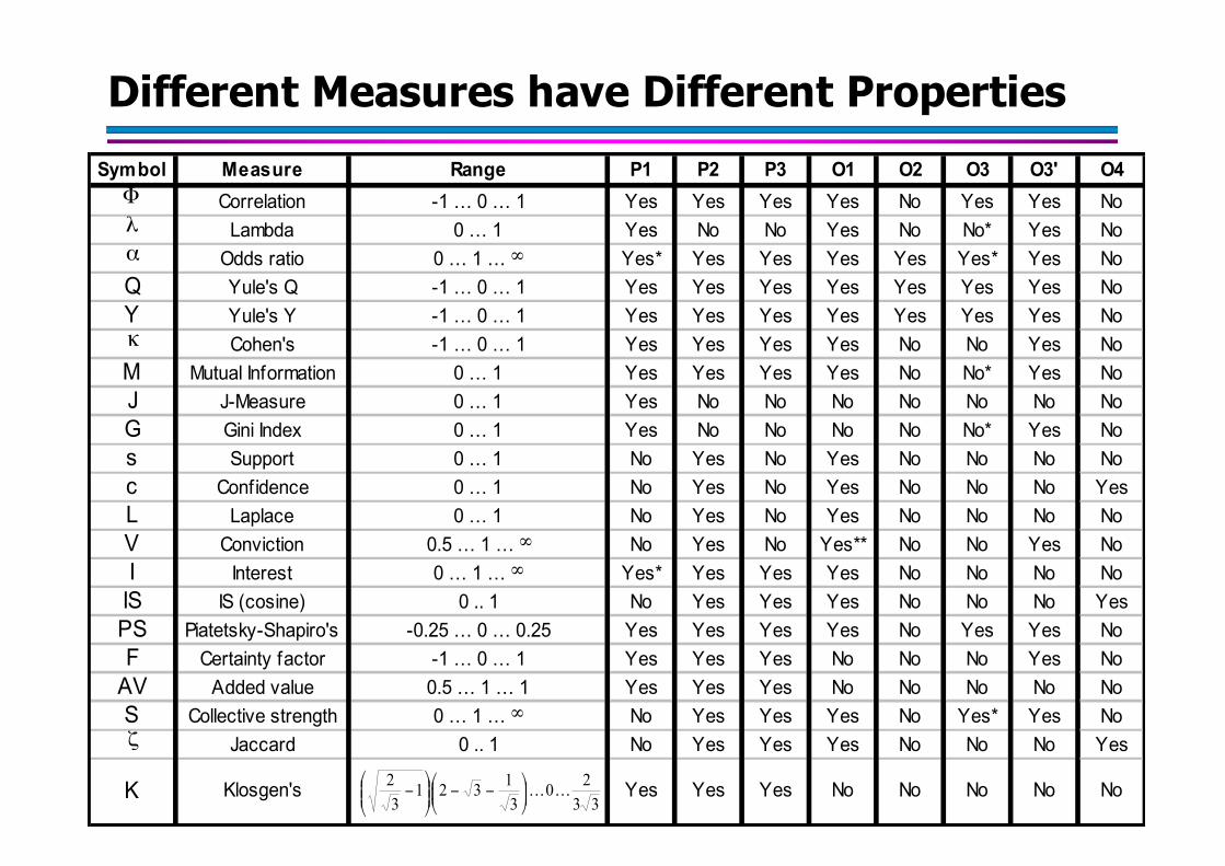
There are lots of measures proposed in the literature
Some measures are good for certain applications, but not for others
What criteria should we use to determine whether a measure is good or bad?
What about Apriori-style support based pruning? How does it affect these measures?
© Tan,Steinbach, Kumar Introduction to Data Mining 4/18/2004 ‹#›
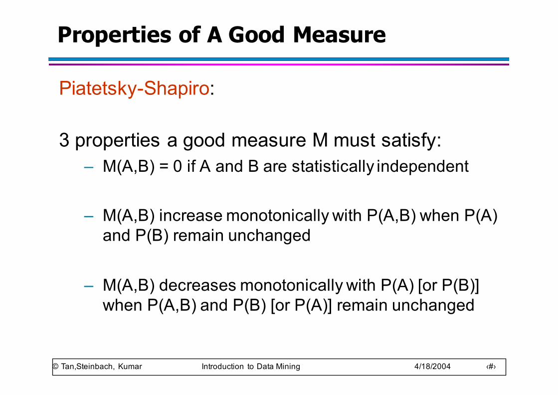
Properties of A Good Measure
Piatetsky-Shapiro:
3 properties a good measure M must satisfy:– M(A,B) = 0 if A and B are statistically independent
– M(A,B) increase monotonically with P(A,B) when P(A) and P(B) remain unchanged
– M(A,B) decreases monotonically with P(A) [or P(B)] when P(A,B) and P(B) [or P(A)] remain unchanged
© Tan,Steinbach, Kumar Introduction to Data Mining 4/18/2004 ‹#›
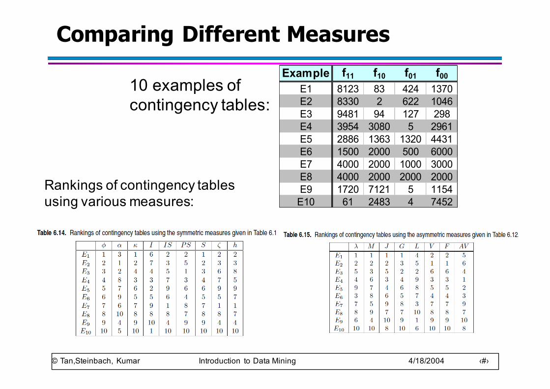
Comparing Different MeasuresExample f11 f10 f01 f00
E1 8123 83 424 1370E2 8330 2 622 1046E3 9481 94 127 298E4 3954 3080 5 2961E5 2886 1363 1320 4431E6 1500 2000 500 6000E7 4000 2000 1000 3000E8 4000 2000 2000 2000E9 1720 7121 5 1154E10 61 2483 4 7452
10 examples of contingency tables:
Rankings of contingency tables using various measures:
© Tan,Steinbach, Kumar Introduction to Data Mining 4/18/2004 ‹#›
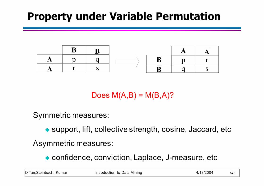
Property under Variable Permutation
B B A p q A r s
A A B p r B q s
Does M(A,B) = M(B,A)?
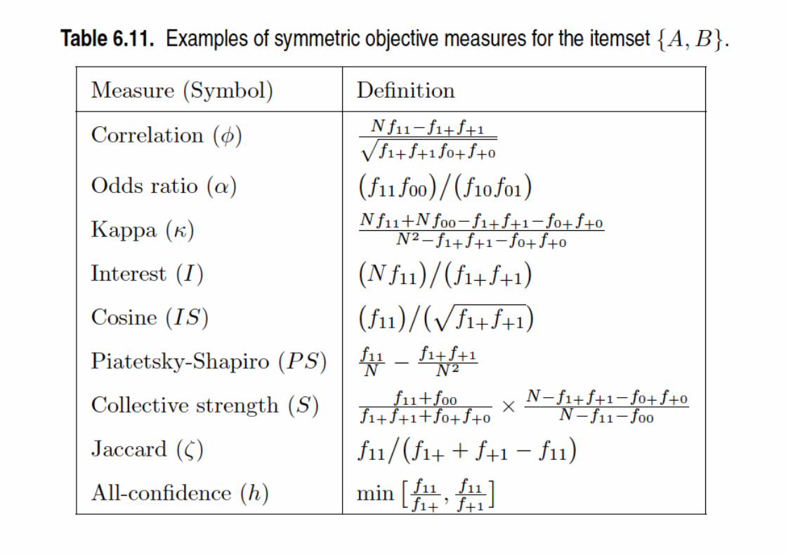
Symmetric measures:
◆ support, lift, collective strength, cosine, Jaccard, etc
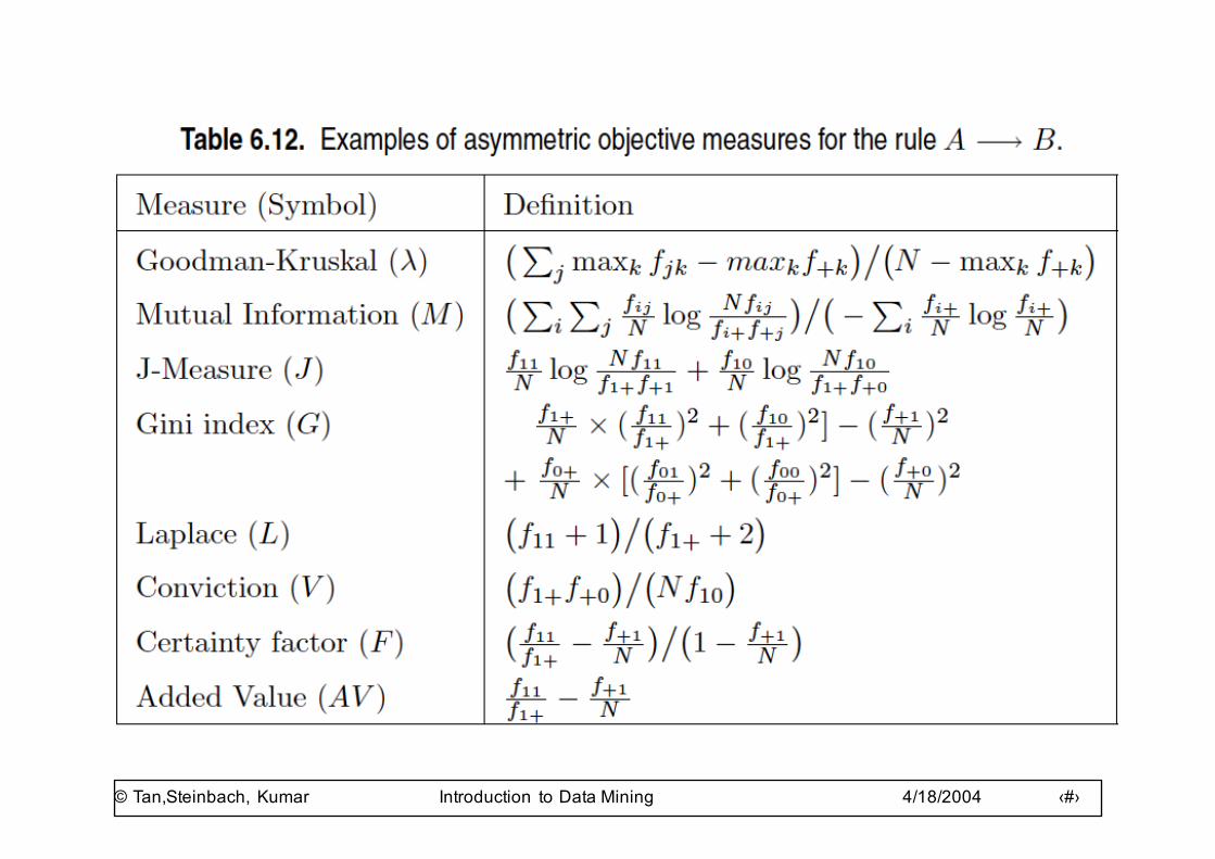
Asymmetric measures:
◆ confidence, conviction, Laplace, J-measure, etc
© Tan,Steinbach, Kumar Introduction to Data Mining 4/18/2004 ‹#›
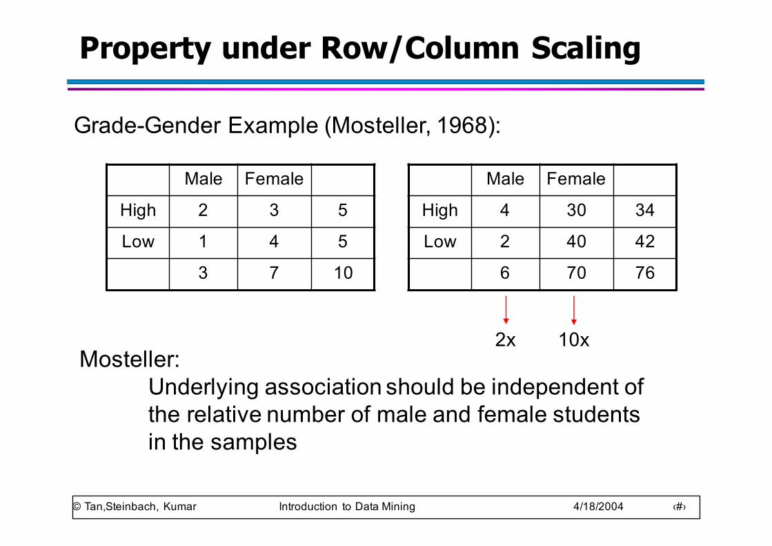
Property under Row/Column Scaling
Male Female
High 2 3 5
Low 1 4 5
3 7 10
Male Female
High 4 30 34
Low 2 40 42
6 70 76
Grade-Gender Example (Mosteller, 1968):
Mosteller: Underlying association should be independent ofthe relative number of male and female studentsin the samples
2x 10x
© Tan,Steinbach, Kumar Introduction to Data Mining 4/18/2004 ‹#›
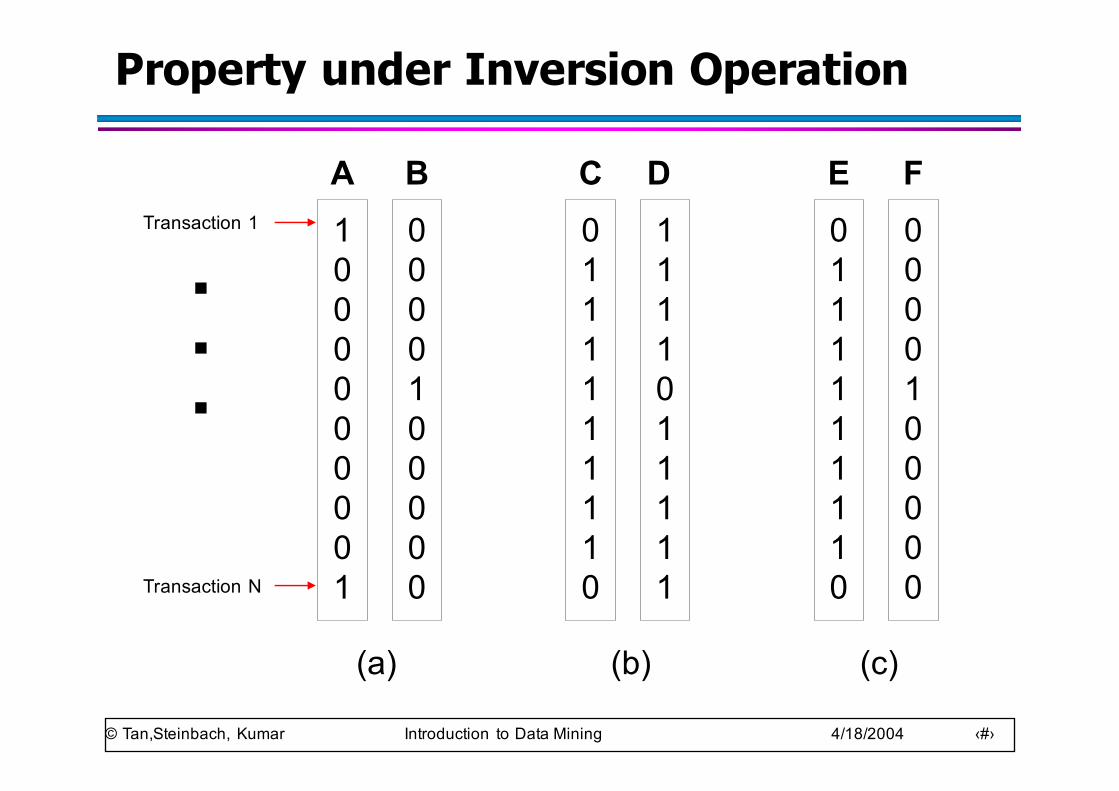
Property under Inversion Operation
1000000001
0000100000
0111111110
1111011111
A B C D
(a) (b)
0111111110
0000100000
(c)
E FTransaction 1
Transaction N
.
.
.
© Tan,Steinbach, Kumar Introduction to Data Mining 4/18/2004 ‹#›
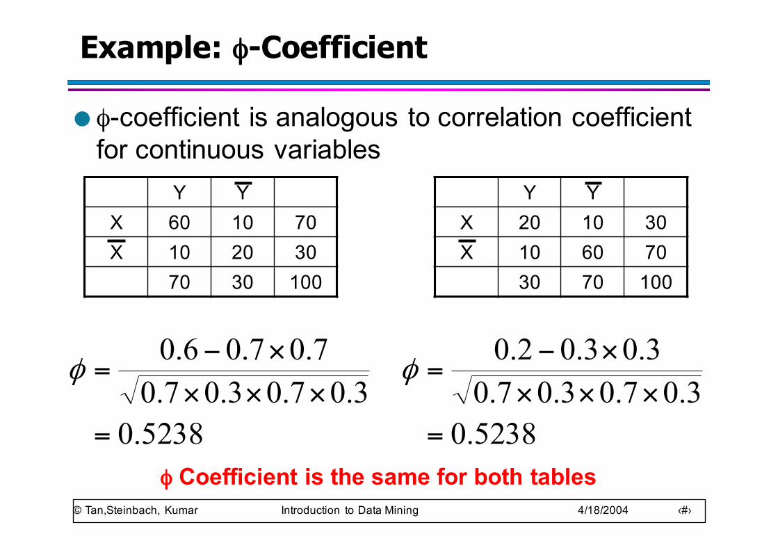
Example: φ-Coefficient
● φ-coefficient is analogous to correlation coefficient for continuous variables
Y YX 60 10 70X 10 20 30
70 30 100
Y YX 20 10 30X 10 60 70
30 70 100
5238.03.07.03.07.0
7.07.06.0
=×××
×−=φ
φ Coefficient is the same for both tables5238.0
3.07.03.07.03.03.02.0
=×××
×−=φ
© Tan,Steinbach, Kumar Introduction to Data Mining 4/18/2004 ‹#›
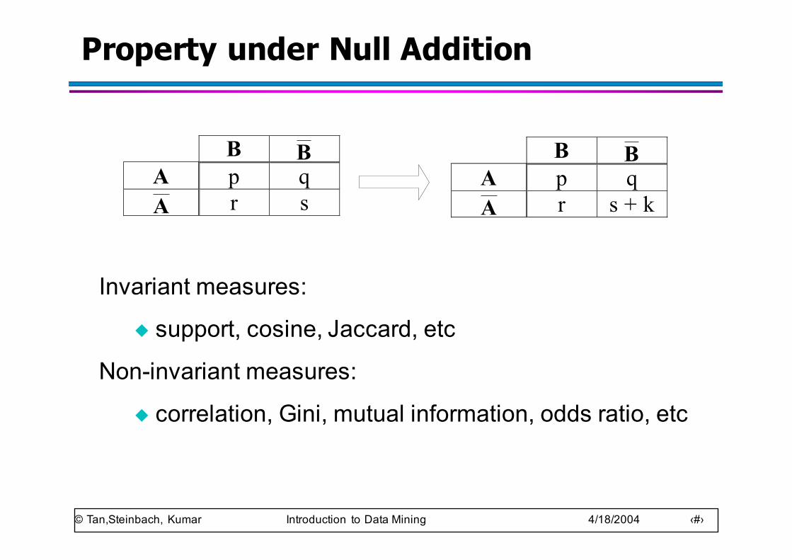
Property under Null Addition
B B A p q A r s
B B A p q A r s + k
Invariant measures:
◆ support, cosine, Jaccard, etc
Non-invariant measures:
◆ correlation, Gini, mutual information, odds ratio, etc
© Tan,Steinbach, Kumar Introduction to Data Mining 4/18/2004 ‹#›
Different Measures have Different PropertiesSymbol Measure Range P1 P2 P3 O1 O2 O3 O3' O4Φ Correlation -1 … 0 … 1 Yes Yes Yes Yes No Yes Yes Noλ Lambda 0 … 1 Yes No No Yes No No* Yes Noα Odds ratio 0 … 1 … ∞ Yes* Yes Yes Yes Yes Yes* Yes NoQ Yule's Q -1 … 0 … 1 Yes Yes Yes Yes Yes Yes Yes NoY Yule's Y -1 … 0 … 1 Yes Yes Yes Yes Yes Yes Yes Noκ Cohen's -1 … 0 … 1 Yes Yes Yes Yes No No Yes NoM Mutual Information 0 … 1 Yes Yes Yes Yes No No* Yes NoJ J-Measure 0 … 1 Yes No No No No No No NoG Gini Index 0 … 1 Yes No No No No No* Yes Nos Support 0 … 1 No Yes No Yes No No No Noc Confidence 0 … 1 No Yes No Yes No No No YesL Laplace 0 … 1 No Yes No Yes No No No NoV Conviction 0.5 … 1 … ∞ No Yes No Yes** No No Yes NoI Interest 0 … 1 … ∞ Yes* Yes Yes Yes No No No No
IS IS (cosine) 0 .. 1 No Yes Yes Yes No No No YesPS Piatetsky-Shapiro's -0.25 … 0 … 0.25 Yes Yes Yes Yes No Yes Yes NoF Certainty factor -1 … 0 … 1 Yes Yes Yes No No No Yes No
AV Added value 0.5 … 1 … 1 Yes Yes Yes No No No No NoS Collective strength 0 … 1 … ∞ No Yes Yes Yes No Yes* Yes Noζ Jaccard 0 .. 1 No Yes Yes Yes No No No Yes
K Klosgen's Yes Yes Yes No No No No No3320
31321
32 !!⎟⎟
⎠
⎞⎜⎜⎝
⎛−−⎟⎟
⎠
⎞⎜⎜⎝
⎛−
© Tan,Steinbach, Kumar Introduction to Data Mining 4/18/2004 ‹#›
Support-based Pruning
● Most of the association rule mining algorithms use support measure to prune rules and itemsets
● Study effect of support pruning on correlation of itemsets
– Generate 10000 random contingency tables– Compute support and pairwise correlation for each
table– Apply support-based pruning and examine the tables
that are removed
© Tan,Steinbach, Kumar Introduction to Data Mining 4/18/2004 ‹#›
Effect of Support-based Pruning
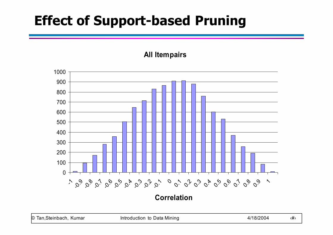
All Itempairs
0100
200300400
500600700800
9001000
-1 -0.9-0.8-0.7-0.6-0.5-0.4-0.3-0.2-0.1 0 0.1 0.2 0.3 0.4 0.5 0.6 0.7 0.8 0.9 1
Correlation
© Tan,Steinbach, Kumar Introduction to Data Mining 4/18/2004 ‹#›
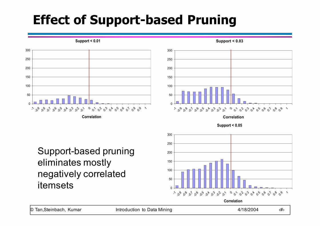
Effect of Support-based PruningSupport < 0.01
0
50
100
150
200
250
300
-1 -0.9-0.8-0.7-0.6-0.5-0.4-0.3-0.2-0.1 0 0.1 0.2 0.3 0.4 0.5 0.6 0.7 0.8 0.9 1
Correlation
Support < 0.03
0
50
100
150
200
250
300
-1 -0.9-0.8-0.7-0.6-0.5-0.4-0.3-0.2-0.1 0 0.1 0.2 0.3 0.4 0.5 0.6 0.7 0.8 0.9 1
Correlation
Support < 0.05
0
50
100
150
200
250
300
-1 -0.9-0.8-0.7-0.6-0.5-0.4-0.3-0.2-0.1 0 0.1 0.2 0.3 0.4 0.5 0.6 0.7 0.8 0.9 1
Correlation
Support-based pruning eliminates mostly negatively correlated itemsets
© Tan,Steinbach, Kumar Introduction to Data Mining 4/18/2004 ‹#›
Effect of Support-based Pruning
● Investigate how support-based pruning affects other measures
● Steps:– Generate 10000 contingency tables– Rank each table according to the different measures– Compute the pair-wise correlation between the
measures
© Tan,Steinbach, Kumar Introduction to Data Mining 4/18/2004 ‹#›
Effect of Support-based Pruning
All Pairs (40.14%)
1 2 3 4 5 6 7 8 9 10 11 12 13 14 15 16 17 18 19 20 21
Conviction
Odds ratio
Col Strength
Correlation
Interest
PS
CF
Yule Y
Reliability
Kappa
Klosgen
Yule Q
Confidence
Laplace
IS
Support
Jaccard
Lambda
Gini
J-measure
Mutual Info
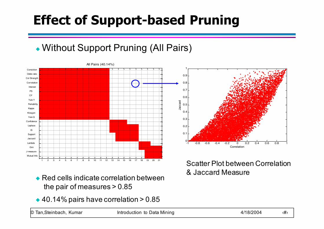
◆ Without Support Pruning (All Pairs)
◆ Red cells indicate correlation betweenthe pair of measures > 0.85
◆ 40.14% pairs have correlation > 0.85
-1 -0.8 -0.6 -0.4 -0.2 0 0.2 0.4 0.6 0.8 10
0.1
0.2
0.3
0.4
0.5
0.6
0.7
0.8
0.9
1
Correlation
Jaccard
Scatter Plot between Correlation & Jaccard Measure
© Tan,Steinbach, Kumar Introduction to Data Mining 4/18/2004 ‹#›
Effect of Support-based Pruning
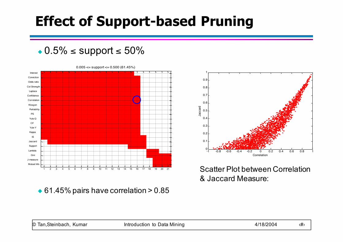
◆ 0.5% ≤ support ≤ 50%
◆ 61.45% pairs have correlation > 0.85
0.005 <= support <= 0.500 (61.45%)
1 2 3 4 5 6 7 8 9 10 11 12 13 14 15 16 17 18 19 20 21
Interest
Conviction
Odds ratio
Col Strength
Laplace
Confidence
Correlation
Klosgen
Reliability
PS
Yule Q
CF
Yule Y
Kappa
IS
Jaccard
Support
Lambda
Gini
J-measure
Mutual Info
-1 -0.8 -0.6 -0.4 -0.2 0 0.2 0.4 0.6 0.8 10
0.1
0.2
0.3
0.4
0.5
0.6
0.7
0.8
0.9
1
Correlation
Jaccard
Scatter Plot between Correlation & Jaccard Measure:
© Tan,Steinbach, Kumar Introduction to Data Mining 4/18/2004 ‹#›
0.005 <= support <= 0.300 (76.42%)
1 2 3 4 5 6 7 8 9 10 11 12 13 14 15 16 17 18 19 20 21
Support
Interest
Reliability
Conviction
Yule Q
Odds ratio
Confidence
CF
Yule Y
Kappa
Correlation
Col Strength
IS
Jaccard
Laplace
PS
Klosgen
Lambda
Mutual Info
Gini
J-measure
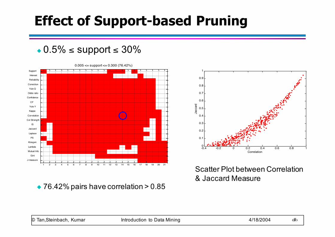
Effect of Support-based Pruning
◆ 0.5% ≤ support ≤ 30%
◆ 76.42% pairs have correlation > 0.85
-0.4 -0.2 0 0.2 0.4 0.6 0.8 10
0.1
0.2
0.3
0.4
0.5
0.6
0.7
0.8
0.9
1
Correlation
Jaccard
Scatter Plot between Correlation & Jaccard Measure
© Tan,Steinbach, Kumar Introduction to Data Mining 4/18/2004 ‹#›
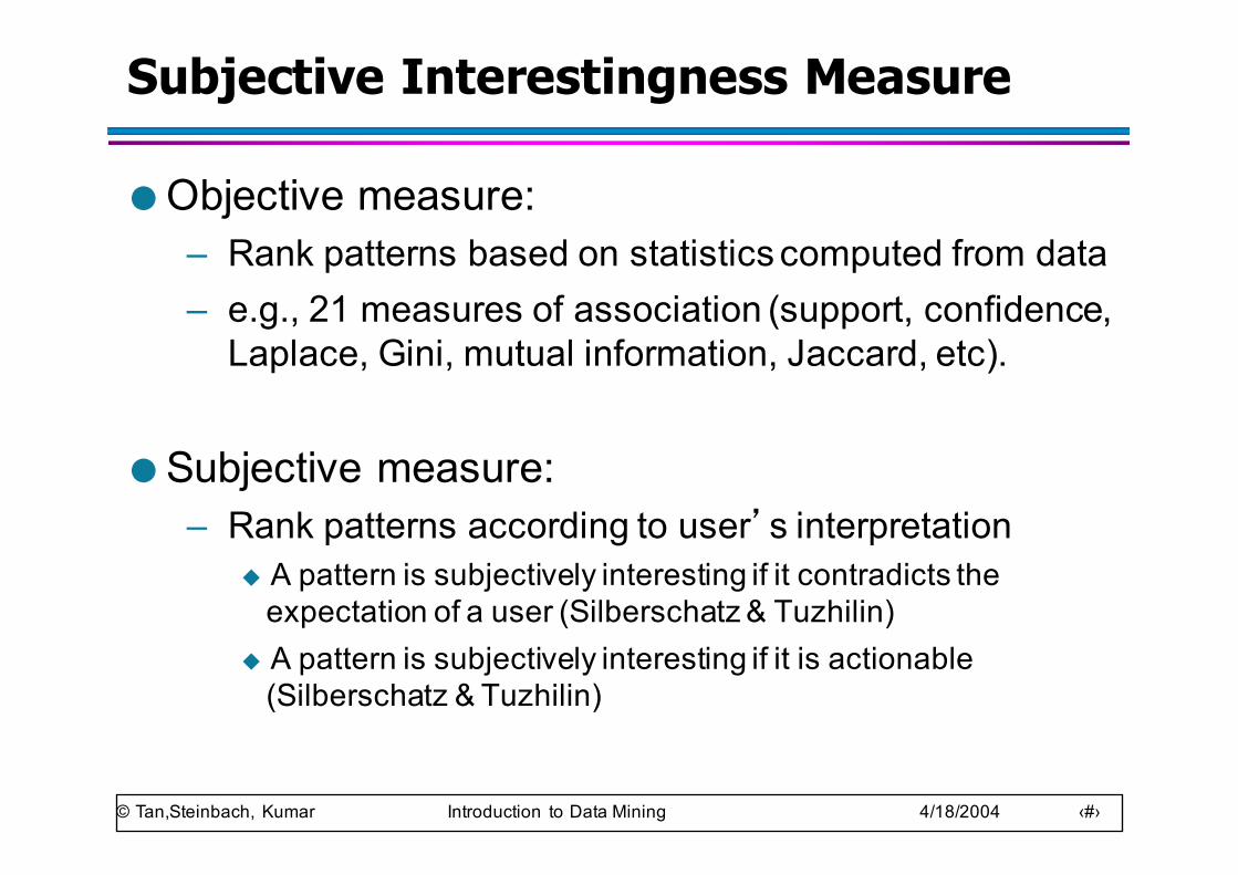
Subjective Interestingness Measure
● Objective measure: – Rank patterns based on statistics computed from data– e.g., 21 measures of association (support, confidence,
Laplace, Gini, mutual information, Jaccard, etc).
● Subjective measure:– Rank patterns according to user’s interpretation
u A pattern is subjectively interesting if it contradicts theexpectation of a user (Silberschatz & Tuzhilin)
u A pattern is subjectively interesting if it is actionable(Silberschatz & Tuzhilin)
© Tan,Steinbach, Kumar Introduction to Data Mining 4/18/2004 ‹#›
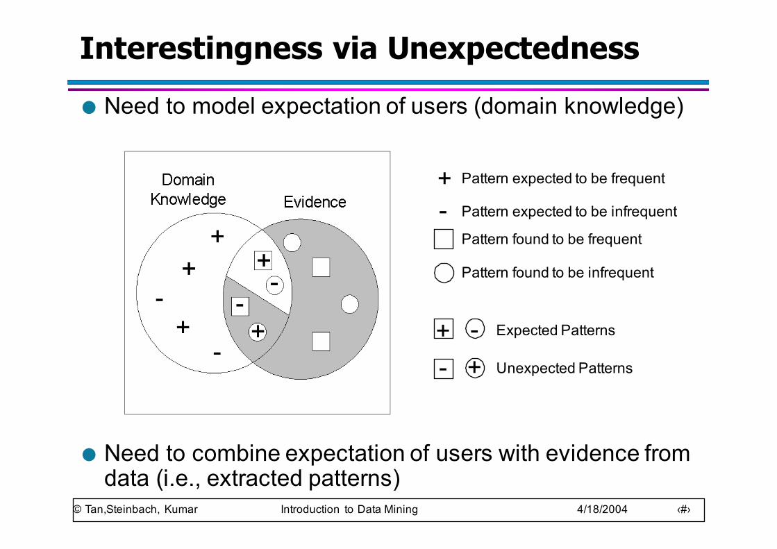
Interestingness via Unexpectedness● Need to model expectation of users (domain knowledge)
● Need to combine expectation of users with evidence from data (i.e., extracted patterns)
+ Pattern expected to be frequent
- Pattern expected to be infrequent
Pattern found to be frequent
Pattern found to be infrequent
+-
Expected Patterns-+ Unexpected Patterns
© Tan,Steinbach, Kumar Introduction to Data Mining 4/18/2004 ‹#›
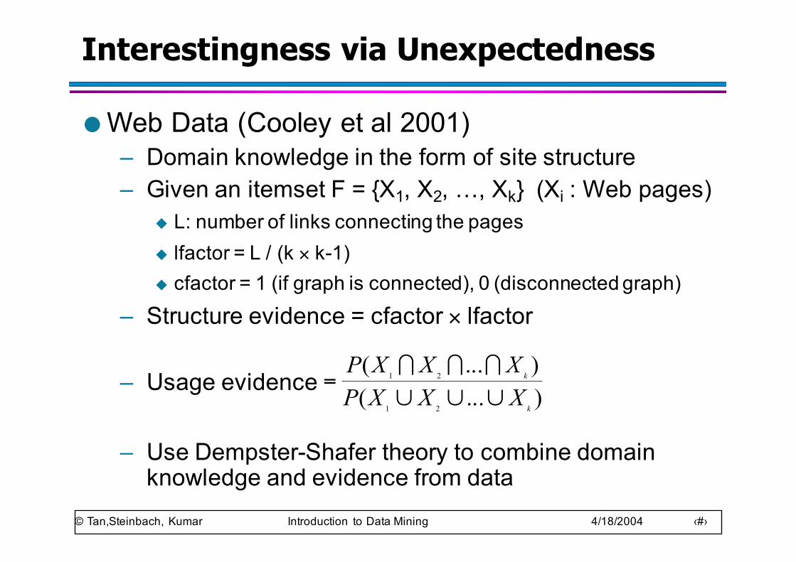
Interestingness via Unexpectedness
● Web Data (Cooley et al 2001)– Domain knowledge in the form of site structure– Given an itemset F = {X1, X2, …, Xk} (Xi : Web pages)
u L: number of links connecting the pages u lfactor = L / (k × k-1)u cfactor = 1 (if graph is connected), 0 (disconnected graph)
– Structure evidence = cfactor × lfactor
– Usage evidence
– Use Dempster-Shafer theory to combine domain knowledge and evidence from data
)...()...(
21
21
k
k
XXXPXXXP
∪∪∪=
!!!
© Tan,Steinbach, Kumar Introduction to Data Mining 4/18/2004 ‹#›
Additionallinks
• http://en.wikipedia.org/wiki/Data_mining• http://www.dataminingarticles.com/association-rules-algorithms.html
• http://www.kdnuggets.com/