National Weather Service National Centers for Environmental Prediction

Technical Procedures Bulletin

Subject: A Variational Wave Height Data Assimilation System for NCEP Operational Wave Models

Series No. MMAB/2004-04 August 6, 2004 MMAB, Environmental Modeling Center, Camp Springs, MD 20746-4304 THIS IS THE FIRST TPB ON THIS SUBJECT. This bulletin, prepared by H. S. Chen, D. Behringer, L. D. Burroughs, and H. L. Tolman, describes a variational wave data assimilation system for use with NCEP operational wave models. Since it became operational in May 2000, The NOAA WAVEWATCH-III (NWW3) suite of wave models has produced forecast waves reasonably well, even though it does not use any observed wave data in the model computations. Recent studies indicate that model results can be considerably improved if observed data are assimilated into the model. Therefore, we have developed an assimilation system for the NWW3. Two types of data are used in the system: satellite altimetry data and buoy wave height data. Both types of data are available in a timely manner. These observed data, when assimilated into the model, give better wave hindcasts, which in turn improve wave forecasts to some degree. The data assimilation has significantly improved NWW3 wave forecasts within the first 12 hours, moderately improved forecasts between 12 and 24 hours, and had little impact on wave forecasts after 24 hours. The data assimilation system was implemented in the Summer of 2004.

National Oceanic and Atmospheric Administration National Weather Service

A VARIATIONAL WAVE HEIGHT DATA ASSIMILATION SYSTEM FOR NCEP OPERATIONAL WAVE MODELS1

By

H.S. Chen2, D. Behringer, L. D. Burroughs, and H. L. Tolman3,

1. Introduction Since it became operational in May 2000, The NOAA WAVEWATCH-III (NWW3) suite of wave models has produced forecast waves reasonably well, even though no observed wave data are used in the model computations. Part of the reason for these good wave forecasts is due to the fact that more realistic analysis wind fields (as opposed to the forecast wind fields) are used in the wave hindcast cycle to generate more realistic initial conditions, which are necessary for each wave cycle. However, the initial conditions can be improved further by assimilating available observed wave information into the model calculation during the hindcast cycle to correct the model waves; thereby, making it possible to produce improved wave forecasts. In this study, we have developed an assimilation system for the NWW3. Two types of data are used in the system: buoy and satellite altimetry wave height data. Both types of data are available in a timely manner. These observed data, when assimilated into the model, give better wave hindcasts, which, in turn, improve wave forecasts to some degree. In fact, the data assimilation has significantly improved NWW3 wave forecasts within the first 12 hours, moderately improved forecasts between 12 and 24 hours, and had little impact on wave forecasts after 24 hours. The data assimilation system was implemented in the Summer of 2004. This TPB describes the NWW3 briefly, to let the reader know the basics of the NWW3 and at which hindcast hours we perform data assimilation. Next, we describe the theory and algorithm used in the data assimilation scheme used in the NWW3. Finally, we evaluate the results of assimilating observed data into the NWW3. 2. Global Ocean Wave Model, NWW3 NWW3 is a NCEP operational wave model that provides a hindcast and forecasts of wave directional spectra and other wave parameters such as wave heights, directions and periods for the global ocean. The model has the following salient features: it uses a third order finite difference scheme combined the ULTIMATE limiter to solve wave propagation; it has additional diffusion terms; and it incorporates the Chalikov formulation for wave generation and the Tolman and Chalikov formulation for wave dissipation. The model uses a spatial grid resolution of 1.00 by 1.25 degrees in latitude and longitude and a spectral resolution of 25 frequencies from 0.04177 Hz (23.94 s) to 0.41145 Hz (2.43 s) with each incremental frequency being 1.1 times the previous frequency and 24 directional bins, each of 15 degrees. The maximum time step is one hour. The wind forcing is derived from 10 m winds derived from the NCEP Global Forecast System (GFS). The NWW3 computer code has been constantly optimized and fully utilizes the advantages of the Massively Parallel Processing (MPP) IBM-RS/6000-SP computer, making the model calculation more efficient. The model runs four times daily at the 00, 06, 12 and 18 UTC cycles and produces a 6-hour wave hindcast out to 180-hour wave forecast. We perform data assimilation hourly in the 6 hindcast hours and first few hours of the forecast. These wave products are posted and updated every 6 hours at the website,

http://polar.ncep.noaa.gov/waves The reader can also find detailed information on the NWW3 at this website. The NWW3 is a directional wave spectral model that provides forecasts of the directional wave spectrum at each computational grid point. Each of these directional wave spectra is then processed to provide wave 1 MMAB Contribution No. 239 2 H. S. Chen L. D. Burroughs and D. Behringer work for NCEP.

23 H. L. Tolman works for SAIC.

parameters such as significant wave height, peak wave period and direction, etc. From a data assimilation point of view, the most desirable data would be those provided by sensors that are capable of measuring the directional wave spectrum. However, very few such measurements are available on an operational basis. Several one-dimensional frequency spectral data are available from many fixed buoys, but these are mostly deployed in coastal waters. But the satellite born altimeters provide measurements of significant wave heights and their data coverage is global. Since the altimeter data represent a significant majority of available wave height data, the assimilation procedure employed here uses only the significant wave height data for assimilation into the wave model. Some details on the variational data assimilation scheme used are given in the next section. 3. Variational Data Assimilation The purpose of a data assimilation applied to ocean waves is to produce the best representation of the true wave field by distributing observed wave data into the model wave field. A variational data assimilation technique is employed. Its scheme was developed by Derber and Rosati (1989) and Behringer (1994, 1998). (Hereafter, we refer to this data assimilation scheme as the DRB scheme) The DRB scheme adopts the functional formulated by Lorenc (1986). It is an objective analysis procedure. This scheme has previously been applied to the sea surface temperature (SST) field by Derber and Rosati (1989), Behringer, et al. (1998) and Kelly, et al. (1999), and also to the sea surface height field by Behringer (1994). 3.1 Lorenc's Functional Without loss of generality, we assume the physical parameter to be studied is the significant wave height η, and its observed data are to be assimilated to the model waves. In the wave hindcast and nowcast, there are three η fields (or arrays) used: (1) the model simulated ηm, also referred to as the first guess or the background estimate, (2) the observed ηo at the observation sites, and (3) the analysis ηa, also referred to as the true value yet to be found. We further define the array of the observation increments xo at the observation sites,

xo = ηo - ηm and the array of the analysis increments x which is also referred to as the correction field,

x = ηa - ηm Following Lorenc (1986), the functional J is, (1) (2)

J = ½ xT E-1 x + ½ [K(x)-xo]T F-1 [K(x)-xo] where the superscripts T and -1 stand for the transpose of the vector and the inverse of the matrix respectively, E is the NxN model error covariance matrix, K is an interpolation operator from grid points to observation locations, and F is the M×M observational error covariance matrix. M is the number of the observations and N the number of the model points. K is assumed to be a linear operator for the field of the wave height. The first term (1) on the right of the functional is a measure of the fit of the model ηm weighted by the inverse of the model error covariance matrix to the corrected field ηa. The second term (2) is a fit of the observations ηo weighted by the inverse of the observational error covariance matrix to the corrected field ηa. For a larger E, the influence of the model ηm to the final analysis ηa diminishes. By the same token, for a larger F, the influence of the observed ηo to ηa also diminishes. 3.2 Model error covariance matrix E

3

The goal of the analysis procedure is to spatially distribute the observational increments xo to the model field. The spatial structure of E can serve this purpose, and it is considered the most important element in the data assimilation algorithm as indicated by Daley (1991). Unfortunately, up to now E is largely unknown for the wave field. Again we shall adopt the same strategy and the simple formulation as Derber (1989) and

Behringer et al (1994, 1998) did in their SST field study. The covariance between any two points separated by a distance r is assumed to have a Gaussian spatial distribution,

A exp[-(r/B)2] where A is the model error variance and B is the estimate of the correlation spatial scale of the model error. The value of A controls the relative weight between the observation and the model. It can be determined by comparing the model data with the observed data. After making allowance for data error, the difference provides an estimate of A. B can be determined using the correlation scale of wave height variability. Generally, A and B vary geographically. After testing many combinations of A (= 0.01, 0.10, 0.25, 0.50 and 1.00 m2) and B (= 2.99, 3.99 and 4.99 degree), we use A = 0.5 m2 and B = 2.99 degrees for the wave field. We note that, in order to reduce computational cost, E is calculated through a Laplacian smoother, not directly from the term, A exp[(-r/B)2]. 3.3 Observational error covariance matrix F Even in the SST field (Behringer, 1994), F is still poorly known and is given in a simple ad hoc fashion. In the wave field, F is nearly unknown, and we shall adopt the same strategy as in the SST. Strictly speaking, F ought to be estimated from measurement errors. Note that here we have not attempted to incorporate errors of representativeness in F. The measurement errors are treated to be spatially uncorrelated and thus F is a diagonal matrix. This makes it easy to calculate F-1. The initial estimates of the diagonal elements of F-1 are set to the reciprocal of an estimate of the observational error variance. Different estimates of the observational error variance are assigned dependent on data type. In wave field, after many tests of various values of F (= 0.04, 0.09, 0.12 and 0.16 m2 for moored and drifting buoy, and 0.09, 0.122 and 0.20 m2 for ERS-2 altimeter), we use 0.09 m2 for moored and drifting buoy and 0.122 m2 for ERS-2 altimeter. It is imperative that, before the observed data can be used in data assimilation, the observed data must pass through a quality control procedure to ensure good quality of the data. 3.4 Algorithm of the DRB Scheme The functional J is used to solve for the analysis increment x, which in turn solves for ηa. The solution can be obtained by minimizing J with respect to x. But to do so is impractical because of computational inefficiency. Instead of directly minimizing J, the DRB scheme employs a preconditioned conjugate gradient algorithm (Gill et al. 1981; Navon and Legler 1987) for the solution. The algorithm attempts to find the solution iteratively. It uses the E matrix for the preconditioning to allow the solution to be found without inverting the E matrix. Now, we define g the derivative of the functional with respect to the corrected field,

g ≡ ∂J/∂x = E-1 x + KT F-1 [K(x)-xo] and

h = E g At the first step, the corrected field x is set to zero. Thus

x1 = 0,

g1 = -KT F-1 xo,

h1 = E g1 where the superscript 1 indicates the first count in the iteration counter. The search directions (d and e) are also set to zero initially,

d0 = 0

4

and

e0 = 0 To find the solution for the correction field x, the following sequence of calculations are performed in each iteration step.

dn = -hn + βn-1 d n-1

en = -gn + βn-1 en-1 fn = en + KT F-1 Kdn

(gn)T hn

αn = (dn)T fn

gn+1 = gn + αn fn

xn+1 = xn + αn dn

hn+1 = E gn+1

(gn+1)T hn+1

βn+1 = (gn)T hn

where superscript n is the iteration counter and is set to one initially. According to Derber et al. (1989) in this algorithm most of the convergence occurs in the first three iterations. Thus, even if only three iterations are used, it does not degrade substantially the results from the assimilation. We note that only the wave height, η, is used in the data assimilation, but the NWW3 calculates, strictly speaking, only the directional wave spectrum ξ(f,θ), where f is the wave frequency and θ the wave direction. Therefore, by considering the wave energy change, we use the relation below, between η and ξ(f,θ), to rescale the spectrum,

ξa(f,θ) = ( ηa/ηm )2 ξm(f,θ) where the subscripts a and m stand for the analysis and the model respectively. 4. Evaluation And Conclusion The goal of the data assimilation is to produce the best representation of the true wave field. Unfortunately, the true wave field is unknown because all wave fields, observed or modeled, always contain errors. This makes evaluation of the results of the data assimilation difficult to be precise. Nevertheless, the best we can do is to treat the observed data as the true data in the evaluation, even though we know that the observed data contain a certain degree of error and are distributed sparsely geographically. Observed wave heights from buoys and the ERS-2 altimeter are used, and they are processed in a one-hour window.

5

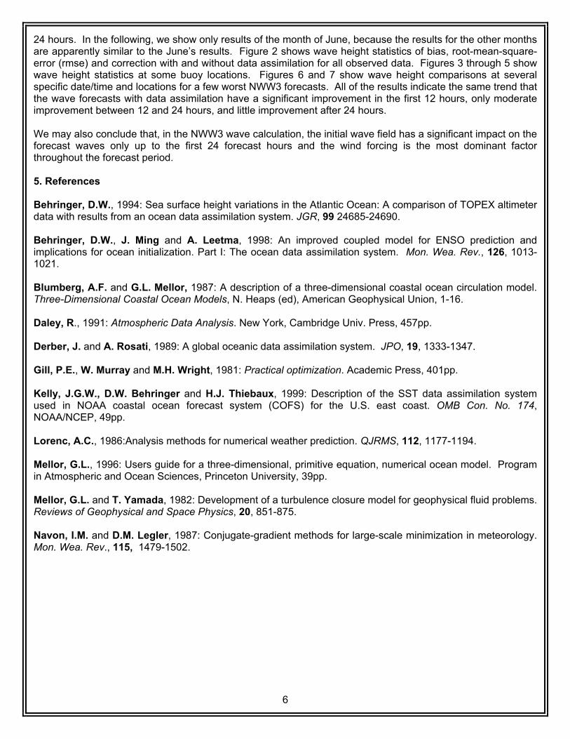
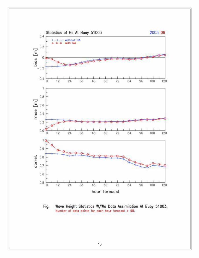
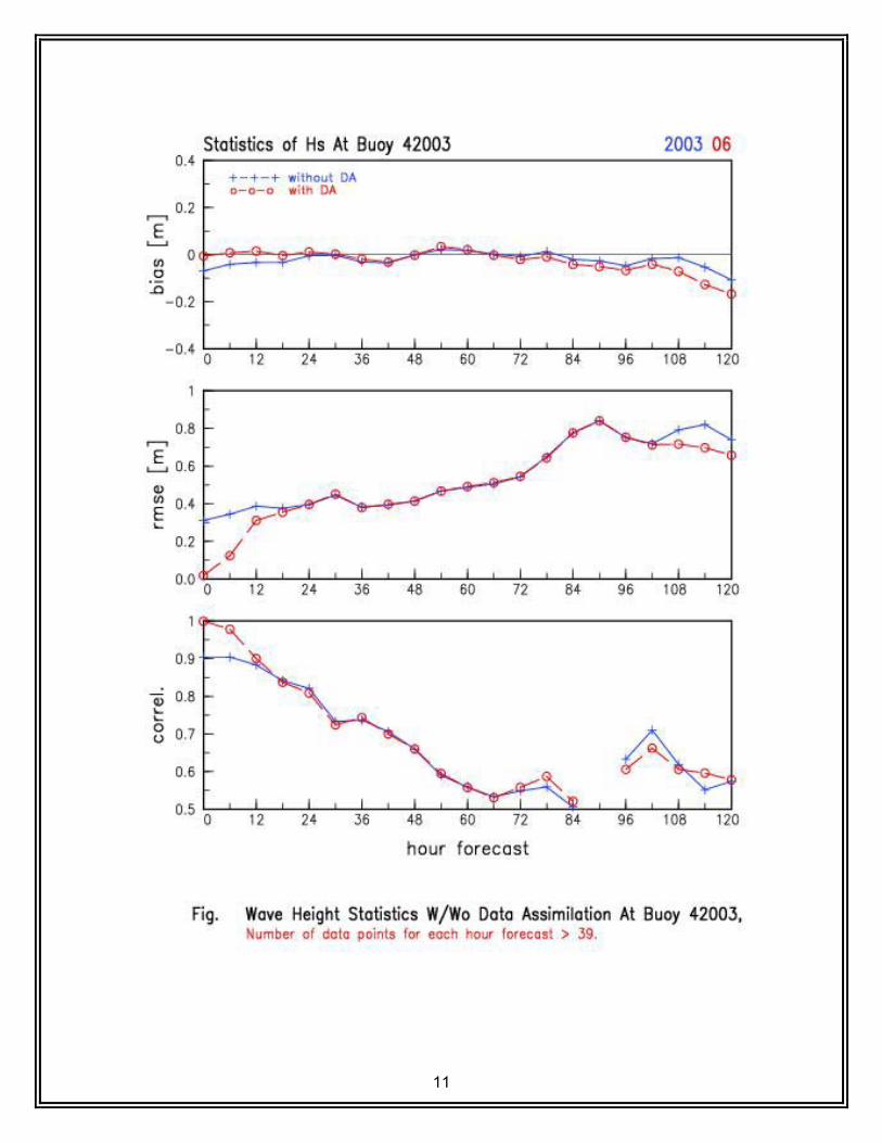
Observed wave height data from the moored buoys and the ERS-2 altimeter are preprocessed in a one-hour window for the 6 hindcast hours and the forecast hours whenever the data are available. These data are then assimilated into the NWW3 waves hourly. From late April through August 2003, the NWW3 with the data assimilation was run in parallel mode for this study. Differences of the wave height fields between the cases with and without the data assimilation are presented here. Figure 1 shows a typical wave height difference at the nowcast hour (or the initial forecast hour). The wave height differences are discernible everywhere near the locations of the observational sites. As shown in the subsequent figures (not shown here), these differences propagate and fade away as the forecast hour goes on, and they become insignificant after about

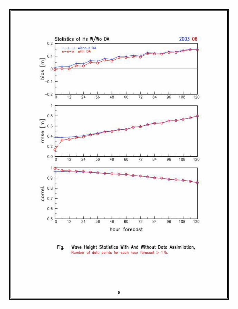
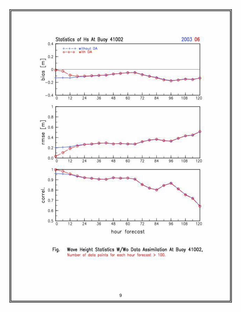
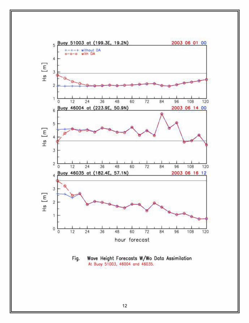
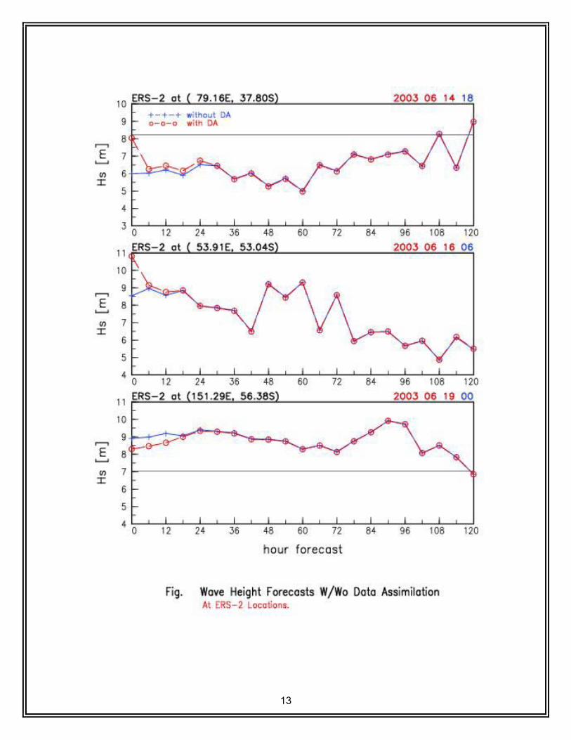
24 hours. In the following, we show only results of the month of June, because the results for the other months are apparently similar to the June’s results. Figure 2 shows wave height statistics of bias, root-mean-square-error (rmse) and correction with and without data assimilation for all observed data. Figures 3 through 5 show wave height statistics at some buoy locations. Figures 6 and 7 show wave height comparisons at several specific date/time and locations for a few worst NWW3 forecasts. All of the results indicate the same trend that the wave forecasts with data assimilation have a significant improvement in the first 12 hours, only moderate improvement between 12 and 24 hours, and little improvement after 24 hours. We may also conclude that, in the NWW3 wave calculation, the initial wave field has a significant impact on the forecast waves only up to the first 24 forecast hours and the wind forcing is the most dominant factor throughout the forecast period. 5. References Behringer, D.W., 1994: Sea surface height variations in the Atlantic Ocean: A comparison of TOPEX altimeter data with results from an ocean data assimilation system. JGR, 99 24685-24690. Behringer, D.W., J. Ming and A. Leetma, 1998: An improved coupled model for ENSO prediction and implications for ocean initialization. Part I: The ocean data assimilation system. Mon. Wea. Rev., 126, 1013-1021. Blumberg, A.F. and G.L. Mellor, 1987: A description of a three-dimensional coastal ocean circulation model. Three-Dimensional Coastal Ocean Models, N. Heaps (ed), American Geophysical Union, 1-16. Daley, R., 1991: Atmospheric Data Analysis. New York, Cambridge Univ. Press, 457pp. Derber, J. and A. Rosati, 1989: A global oceanic data assimilation system. JPO, 19, 1333-1347. Gill, P.E., W. Murray and M.H. Wright, 1981: Practical optimization. Academic Press, 401pp. Kelly, J.G.W., D.W. Behringer and H.J. Thiebaux, 1999: Description of the SST data assimilation system used in NOAA coastal ocean forecast system (COFS) for the U.S. east coast. OMB Con. No. 174, NOAA/NCEP, 49pp. Lorenc, A.C., 1986:Analysis methods for numerical weather prediction. QJRMS, 112, 1177-1194. Mellor, G.L., 1996: Users guide for a three-dimensional, primitive equation, numerical ocean model. Program in Atmospheric and Ocean Sciences, Princeton University, 39pp. Mellor, G.L. and T. Yamada, 1982: Development of a turbulence closure model for geophysical fluid problems. Reviews of Geophysical and Space Physics, 20, 851-875. Navon, I.M. and D.M. Legler, 1987: Conjugate-gradient methods for large-scale minimization in meteorology. Mon. Wea. Rev., 115, 1479-1502.

6

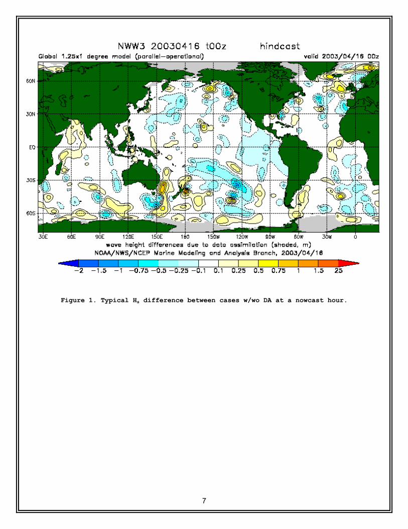
Figure 1. Typical Hs difference between cases w/wo DA at a nowcast hour.

7

8

9

10

11

12

13