Embed Size (px)
Citation preview
A
Presented tothe faculty of the School of Engineering and Applied Science
University of Virginia
in partial fulfillmentof the requirements for the degree
by
Data- and Model-driven Predictive Control: With Applications to Connected Autonomous Vehicles
Dissertation
Doctor of Philosophy
Hassan Jafarzadeh
May 2021
APPROVAL SHEET
This
is submitted in partial fulfillment of the requirementsfor the degree of
Author:
Advisor:
Advisor:
Committee Member:
Committee Member:
Committee Member:
Committee Member:
Committee Member:
Committee Member:
Accepted for the School of Engineering and Applied Science:
Jennifer L. West, School of Engineering and Applied Science
Dissertation
Doctor of Philosophy
Hassan Jafarzadeh
This Dissertation has been read and approved by the examing committee:
Cody H. Fleming
James H. Lambert
Zongli Lin
Abigail A. Flower
T. Donna Chen
May 2021

©Copyright by Hassan Jafarzadeh 2021
All Rights Reserved

Abstract
Traditional techniques for analyzing and developing control laws in safety-
critical applications usually require a precise mathematical model of the sys-
tem. However, there are many control applications where such precise, an-
alytical models can not be derived or are not readily available. Increasingly,
data-driven approaches from machine learning are used in conjunction with
sensor or simulation data in order to address these cases. Such approaches
can be used to identify unmodeled dynamics with high accuracy. However,
an objective that is increasingly prevalent in the literature involves merging or
complementing the analytical approaches from control theory with techniques
from machine learning.
Autonomous systems 1 such as self-driving vehicles, distributed sensor net-
works, aerial drones, and agile robots, need to interact with their environments
that are ever-changing and difficult to model. These and many other applica-
tions motivate the use of data-driven decision-making and control together.
However, if data-driven systems are to be applied in these new settings, it is
critical that they be accompanied by guarantees of safety and reliability, as
failures could be catastrophic.
This dissertation addresses the problems in which there are interactions be-1An autonomous system is one that can achieve a given set of goals in a changing environ-ment – gathering information about the environment and working for an extended period oftime without human control or intervention. In this dissertation, the autonomous systems isnot used in the control theory sense which has the form of x = f(x) and does not involvecontrol input (unforced system)

tween model-based and data-driven systems and develops learning-based
control strategies for the entire system that guarantees safety and optimal-
ity. Applications of these systems can be sough in autonomous networked
mobile systems that are quickly making their way into the marketplace and are
soon expected to serve a wide range of new tasks including package delivery,
cooperatively fighting wildfires, and search and rescue after a natural disaster.
As the number of these systems increases, their performance and capabili-
ties can be greatly enhanced through wireless coordination. Wireless channel
extremely contributes to the optimality and safety of the whole system, but it
is a data-driven factor and there is no explicit mathematical model for it to be
involved in the model-based part, that is mostly model predictive controller.
This dissertation presents two approaches to address the above-mentioned
problem. The first proposed approach is the Gaussian Process-based Model Pre-
dictive Controller (GP-MPC) that leverages Gaussian Processes (GPs) to learn
the variations of the data-driven variable in a defined time horizon. To avoid
a large number of interactions with the environment in the learning process,
the algorithm iterates in the reachable set from the current state to decrease
the size of the kernel matrix and converge to the optimal trajectory faster. To
reduce the computational cost further, an efficient recursive approach is devel-
oped to calculate the inverse of kernel matrix while MPC updates at each time
step.
The second approach is Data-and Model-Driven Predictive Control (DMPC)
which is a data-efficient learning controller that provides an approach to merge
both the model-based (MPC) and data-based systems. DMPC is developed
to solve an MPC problem that deals with an unknown function operating in-
terdependently with the model. It is assumed that the value of the unknown
function is predicted or measured for a given trajectory by an exogenous data-
driven system that works separately from the controller. This algorithm can

cope with very little data and builds its solutions based on the recently gen-
erated solution and improves its cost in each iteration until converging to an
optimal solution, which typically needs only a few trials. Theoretical analysis
for recursive feasibility of the algorithm is presented and it is proved that the
quality of the trajectory does not get worse with each new iteration.
In the end, the developed algorithms are applied to the motion planning of two
connected autonomous vehicles with linear and nonlinear dynamics. The re-
sults illustrate that the controller can create a safe trajectory that not only is
optimal in terms of control effort and highway capacity usage but also results
in a more stable wireless channel with maximum packet delivery rate (PDR).
Keywords: Learning Optimal Control, Model Predictive Control, Data-efficient
Controller, Gaussian Process, Autonomous Vehicles, Connected Vehicles

Acknowledgements
First and foremost, I would like to express my deepest appreciation to my ad-
visor Professor Cody Fleming for his patience, insightful suggestions, and in-
valuable supports. You never stopped encouraging and pushing me forward
throughout my years of study and the process of researching. Your valuable
feedback helped me to sharpen my thinking and brought my work to a higher
level. From the bottom of my heart I would like to say big thank you for your
endless supports.
I would also like to extend my sincere gratitude to my Ph.D. committee mem-
bers for their valuable advice and insightful comments on this dissertation.
A special thanks to my beloved family. Mother and father, words cannot ex-
press how grateful I am for all of the sacrifices that you have made on my be-
half. Your prayer for me was what sustained me thus far and made me who I
am now. Brother and sister, your unconditional love and supports are invalu-
able. You are always there for me and I am forever indebted to you.
Finally and most importantly, I would like to thank my beloved wife Nazanin
for her love and constant supports. I cannot thank you enough for encourag-
ing me throughout this entire journey. You have been my best friend and great
companion from the time you entered my life. I am extremely grateful for your
countless sacrifices, supports and valuable discussions that prevented several
wrong turns and helped me get to this point.

Table of Contents
List of Tables
List of Figures
1 Introduction
2 Problem Background, Motivations and Challenges
2.1 Background . . . . . . . . . . . . . . . . . . . . . . . . . . . . . . .
2.2 Motivations . . . . . . . . . . . . . . . . . . . . . . . . . . . . . . .
2.3 Challenges and existing approaches . . . . . . . . . . . . . . . . .
2.3.1 Perfect wireless channel . . . . . . . . . . . . . . . . . . .
2.3.2 Wireless channel with time-varying delay . . . . . . . . . .
2.3.3 Summary & Conclusions . . . . . . . . . . . . . . . . . . .
2.4 Proposed Methods . . . . . . . . . . . . . . . . . . . . . . . . . .
3 Gaussian Process-based Model Predictive Controller for CAVs
3.1 Introduction . . . . . . . . . . . . . . . . . . . . . . . . . . . . . .
3.2 Background: MPC scheme for CAVs . . . . . . . . . . . . . . . . .

3.2.1 Perfect Communication Channel . . . . . . . . . . . . . .
3.2.2 Imperfect Communication Channel . . . . . . . . . . . . .
3.3 Gaussian Process for CAVs . . . . . . . . . . . . . . . . . . . . . .
3.3.1 Probabilistic Model for Wireless Channel . . . . . . . . . .
3.3.2 Efficient Recursive GP-MPC . . . . . . . . . . . . . . . . .
3.4 Example Scenario - Uncertain Communication Channel . . . . . .
3.5 Conclusions . . . . . . . . . . . . . . . . . . . . . . . . . . . . . .
4 Learning Model Predictive Control for CAVs
4.1 Preliminaries of Learning Model Predictive Control . . . . . . . .
4.1.1 Sampled Safe Set . . . . . . . . . . . . . . . . . . . . . . .
4.1.2 Iteration Cost . . . . . . . . . . . . . . . . . . . . . . . . .
4.1.3 LMPC Formulation . . . . . . . . . . . . . . . . . . . . . .
4.2 Learning Model Predictive Control for CAVs . . . . . . . . . . . .
4.3 Conclusions . . . . . . . . . . . . . . . . . . . . . . . . . . . . . .
5 Data-and Model-Driven Approach to Predictive Control
5.1 Introduction . . . . . . . . . . . . . . . . . . . . . . . . . . . . . .
5.2 Problem Statement . . . . . . . . . . . . . . . . . . . . . . . . . .
5.3 DMPC Approach . . . . . . . . . . . . . . . . . . . . . . . . . . . .
5.3.1 Algorithmic Details . . . . . . . . . . . . . . . . . . . . . .
5.3.2 Theoretical Analysis . . . . . . . . . . . . . . . . . . . . . .

5.4 Implementation Steps . . . . . . . . . . . . . . . . . . . . . . . . .
5.5 Example . . . . . . . . . . . . . . . . . . . . . . . . . . . . . . . . .
5.5.1 Linear Dynamical System . . . . . . . . . . . . . . . . . . .
5.5.2 Nonlinear System . . . . . . . . . . . . . . . . . . . . . . .
5.6 Conclusions . . . . . . . . . . . . . . . . . . . . . . . . . . . . . .
6 Summary of Contributions & Future Work
6.1 Summary of Contributions . . . . . . . . . . . . . . . . . . . . . .
6.1.1 Gaussian Process-based Model Predictive Controller . . .
6.1.2 Learning Model Predictive Control . . . . . . . . . . . . . .
6.1.3 Data-and Model-Driven Predictive Control . . . . . . . . .
6.2 User guide for developed algorithms . . . . . . . . . . . . . . . .
6.3 Future work . . . . . . . . . . . . . . . . . . . . . . . . . . . . . . .
6.3.1 Iterative GP-MPC . . . . . . . . . . . . . . . . . . . . . . .
6.3.2 Generating the initial solution for DMPC . . . . . . . . . .
6.3.3 Escaping Local Optima in DMPC . . . . . . . . . . . . . . .
6.3.4 Optimal control of unknown systems using DMPC . . . .
6.3.5 Notations . . . . . . . . . . . . . . . . . . . . . . . . . . . .

List of Tables
4.1 Scenario and Model Parameters . . . . . . . . . . . . . . . . . . .
6.1 Main Notations . . . . . . . . . . . . . . . . . . . . . . . . . . . . .

List of Figures
2.1 Platoon of heterogeneous vehicles [1] . . . . . . . . . . . . . . . .
3.1 Optimal trajectory of ego vehicle generated by GP-MPC to avoid
a region with a considerable delay time in packet delivery. . . . .
3.2 Optimal control input xt, state xt and inter-vehicular distance dt
over the time horizon. . . . . . . . . . . . . . . . . . . . . . . . . .
4.1 Workflow of the presented Control . . . . . . . . . . . . . . . . .
4.2 Car-following scenario: The ego vehicle should avoid the dead-
zone region (red rectangle) . . . . . . . . . . . . . . . . . . . . . .
4.3 Car-following scenario: The cost of entering into the dead-zone
is not significant in this case . . . . . . . . . . . . . . . . . . . . .
5.1 Scheme of the controller and its relationship with the exoge-
nous system. . . . . . . . . . . . . . . . . . . . . . . . . . . . . . .
5.2 The green area shows the N -step reachable set,RN(x∗,jt ), from
current state, x∗,jt . Controllable set Sjt is illustrated by large blue
dots and dashed purple line segments are the optimal trajec-
tories from current state to available states in controllable set
Sjt . . . . . . . . . . . . . . . . . . . . . . . . . . . . . . . . . . . . .

5.3 DMPC generates two trajectories xjt:t+N |t (solid black) and xjt:t+N |t−1
(dashed green) at time step t of iteration j, and selects best of
them . . . . . . . . . . . . . . . . . . . . . . . . . . . . . . . . . . .
5.4 Trajectory costs in different time steps. Orange: x∗,j−1. Blue:
xj0:N . Green: xj1:N+1. . . . . . . . . . . . . . . . . . . . . . . . . . . .
5.5 The cost of entering to the blue and red area are small and very
big, respectively. The down-left graph shows the cost-to-go vec-
tor for the states of each separate trajectory, that from top (it-
eration 0 or initial trajectory) to down (last iteration) the conver-
gence of trajectories can be seen. The Down-right graph illus-
trates the overall trajectory cost of each trajectory. . . . . . . . .
5.6 Control input ut = [xt yt]T and states xt and yt in the steady state.
5.7 The contour plot of unknown non-convex cost function, i.e.
given in equation (5.54), and local optimal trajectory generated
by DMPC. . . . . . . . . . . . . . . . . . . . . . . . . . . . . . . . .
5.8 Control input ut = [xt yt]T and states xt and yt in the steady
state for the cost function of equation (5.54). . . . . . . . . . . .
5.9 Kinematic Bicycle Model . . . . . . . . . . . . . . . . . . . . . . .
5.10 The contour plot of unknown non-convex cost function, and lo-
cal optimal trajectory generated by DMPC. The down-left graph
shows the cost-to-go vector for the states of each separate tra-
jectory, that from top (iteration 0 or initial trajectory) to down
(last iteration) the convergence of trajectories can be seen. The
Down-right graph illustrates the overall trajectory cost of each
trajectory. . . . . . . . . . . . . . . . . . . . . . . . . . . . . . . . .
5.11 Control input ut = [δt at]T and states ψt and vt in the steady state.

Chapter 1
Introduction
The conventional control approaches usually need a precise physical model
of the system to develop an optimal and safe controller and also analyze its
characteristics and provide the required guarantees about the optimality, con-
vergence and safety [2–4]. Nevertheless, these mathematical models are not
always available, and only data-driven techniques such as deep learning meth-
ods, Gaussian Processes, statistical methods, and etc are used to describe
the behaviour of these systems. These techniques can be utilized to identify
the unmodeled system with a high accuracy, but challenges appears when we
need some guarantees about the safety, stability and optimality about the sys-
tem and the provided solutions.
Model Predictive Control (MPC) is a methodology in the control area that is
used broadly to control the autonomous systems. To apply this method, the
exact dynamical system is required. Also, the model requires us to add the lim-
itations on the state and control vectors as equality or inequality constraints
into the model. And finally, the cost function steers the state of the system
from the initial to the terminal state. All of these components require explicit
mathematical definitions. However, in some applications these relationships
can not be defined easily.

Connected Autonomous Vehicles (CAVs) are well-known systems in this group
and will be used as an application throughout the dissertation to make the
explanations of the developed algorithms more understandable. CAVs have
shown a great potential to improve both highway throughput and fuel effi-
ciency by traveling nearly bumper-to-bumper while guaranteeing safety. Wire-
less coordination could enable mobile systems to reach high-performance
states that would not otherwise be safe (closer distances, higher speeds, etc).
In the connected mobile systems, especially in CAVs, the main challenge is
to capture the interdependence between mobility, wireless, and safety. The
established communication channel between the vehicles of a platoon can
be easily influenced by numerous factors e.g. surrounding environment, the
states of the connected vehicles and etc. Between these factors, the motion
policies generated by the agent’s controller can profoundly affect the state of
the wireless channel. Inevitably, a poor and imperfect communication channel
results in a sequence of conservative control inputs (because of the safety
concerns) that impact the overall performance.
Connected, autonomous vehicles (CAVs) have the potential to identify, collect,
process, exchange, and transmit real-time data leading to greater awareness
of – and response to – events, threats, and imminent hazards within the ve-
hicle’s environment. At the core of this concept is a networked environment
supporting very high speed interactions among vehicles (V2V), and between
vehicles and infrastructure components (V2I) to enable numerous safety and
mobility applications. When combined with automated vehicle-safety appli-
cations, vehicle connectivity provides the ability to respond and react in ways
that drivers cannot, or cannot in a timely fashion, significantly increasing the
effectiveness of crash prevention and mitigation. Connected Autonomous Ve-
hicles (CAVs) are the advanced generation of the driverless cars that are of
interest to many researchers in this field. One application of CAVs involves Co-

operative Adaptive Cruise Control (CACC), in which the following vehicle not
only localizes the preceding vehicle via on-board sensing, but also receives in-
formation of the preceding vehicles’ current state(s) through a wireless chan-
nel [5]. CACC is an extension to ACC (Adaptive Cruise Control) that is capable
of applying acceleration/deceleration depending on the existence of a preced-
ing vehicle in a certain range. ACC is one of the first concepts enabling au-
tomation to involve a safety concern (i.e. time-to-collision) in its action policy.
Real-time control algorithms, e.g. Model Predictive Control (MPC), provide
a foundation to significantly improve CACC performance. As an Advanced
driver-assistance systems (ADAS), MPC involves generating a sequence of
motion policies for some number of time steps in the future and executing a
subset of this sequence in a receding fashion. Predicting the optimal trajec-
tory into the future benefits the system in different ways, such as providing
safety guarantees (e.g. obstacle avoidance) and minimizing control effort. Fur-
thermore, in the context of CAVs, the predicted motion policy can be shared
via a communication channel with the other vehicles. Being aware of future
vehicle states allows better agility, maneuverability, safety, and optimality [6].
There is a growing literature on MPC in connected vehicle applications [7–9].
However, most of this work assumes a perfect communication channel, mean-
ing that an ego (following) vehicle receives packets from the preceding vehicle
with no dropouts or delay. However, communication delays present a chal-
lenge, especially in vehicle-to-vehicle, or V2V, communication systems, which
are characterized by a dynamic environment, high mobility, and low antenna
heights/power on the transceivers (e.g. between vehicles and roadside units,
telecommunications, etc) [10]. Communication delay can impact the perfor-
mance of vehicle platoons in myriad ways. [11] studies these effects and the
reported results show that string stability is seriously compromised by the
communication delay introduced by the network. They assume a constant

communication delay (i.e. a very benign delay) and propose a simple fix to pre-
serve string stability that is not optimal. The sub-optimality of their approach
comes from the fact that controller designs do not explicitly account for delay
in the communication links. In practice a wireless channel inevitably contains
random delays, and packet losses vary based on the surrounding environment.
Therefore, an approach of multiple time-varying delays was considered in [12],
which implements adaptive feedback gains to compensate for the errors origi-
nated from outdated packets, provides upper bound estimates for time delays,
and examines stability conditions using Linear Matrix Inequality techniques.
However, little work has been done on the effect of uncertainty of communi-
cation channel on the control policy of CAVs, and to our knowledge none have
considered the wireless network itself as a dynamic variable. Typically, when
the policy of a connected vehicle is optimized over a time horizon based on a
given behaviour of the channel, it is assumed that the network will not vary by
changing the state of the vehicle. However, the states of the communicating
vehicles are important factors that influence the wireless channel.
States of the vehicle and wireless communication channel (e.g. PDR, or Packet
Delivery Rate) are two interdependent variables, where changing either will af-
fect the other [6]. The ego vehicle should not only take into account the cost of
control effort and its longitudinal distance from the preceding vehicle, but also
the state of the wireless network should be involved in its controller model.
For instance, the state of the ego vehicle where the communication channel
has zero PDR is not desirable because at this state the ego vehicle will not re-
ceive any packet from the lead vehicle which in turn results in a sequence of
conservative controls (because of the safety concerns) that impacts the over-
all performance. Accordingly, having a more stable wireless channel with a
higher PDR improves the overall performance of the CAVs; however the chal-
lenge is, being data-driven, the wireless communication channel cannot be for-

mulated directly as a straightforward mathematical model to be merged into
the model predictive controller.
This dissertation introduces two novel approaches to involve a data-driven
system in MPC (i.e. a model-based method) to generate a solution that is opti-
mal for the entire system with the applications on connected vehicles:
• GP-MPC (Gaussian Process-based Model Predictive Controller): To con-
sider the PDR in MPC, the Gaussian Processes (GP) is used which is a
model-based method. GP is preferable in this work because the varia-
tions of the environment can be learned and used as a proxy model rep-
resenting the behaviour of the wireless network for a given time horizon.
Also, being a probabilistic method, the uncertainty can be incorporated
into a long-term prediction (time horizon) by using GPs and the impact of
the errors can be reduced [13, 14]. This is a data-efficient approach com-
pared to the model-free methods (e.g. Q-learning or TD-learning) and can
be used without additional interaction with the environment [15]. After
obtaining the proxy model, it can be used in MPC to generate a motion
policy in which the PDR, control effort and the highway capacity usage
are balanced in an optimal way.
• DMPC (Data-and Model-driven Predictive Control): A technique based
on Iterative Learning Control (ILC) is presented that can incorporate an
unknown cost function in MPC to generate the optimal trajectory in a few
trials. The algorithm starts from a given initial trajectory and improves it
by learning from each iteration until converging to an optimal solution.
Iterative Learning Control is typically applied for systems that repeat the
same operation under the same conditions and enables the controller
to learn from previous executions (iterations) to improve its closed-loop
reference tracking performance [16, 17].

The rest of this dissertation is organized as follows. Chapter (2) provides an
overview of the problem’s background, motivations and challenges. Chap-
ter (3) presents Gaussian Process-based Model Predictive Controller (GP-
MPC) for the CAVs in the presence of uncertain wireless channel. Chapter (4)
explains a preliminary version of (Learning Model Predictive Control) LMPC-
based approach for CAVs. In Chapter (5) the presented approach of the pre-
vious chapter is enhanced to overcome its shortcomings, the novel algorithm
is called Data-and Model-driven Predictive Control (DMPC). And finally, Chap-
ter (6) provides a summary of contributions, future work and conclusions to
this dissertation.

Chapter 2
Problem Background, Motivations
and Challenges
2.1 Background
The number of motor vehicles in the world is around one billion and it is in-
creasing rapidly, where it is estimated that this number will be doubled within
the next ten years [18]. By increasing this number, the safety and efficiency re-
lated concerns attract more attention.
On the other hand, recent advances in autonomous driving are becoming in-
creasingly ubiquitous, and Advanced Driving Assistance Systems (ADAS) have
the potential to improve safety and comfort in various driving conditions. Adap-
tive Cruise Control (ACC) is a widely used ADAS module that controls the vehi-
cle longitudinal dynamics. ACC is triggered once a preceding vehicle is de-
tected within a certain distance range from the ego vehicle. ACC automati-
cally maintains a proper minimum safe distance from preceding vehicles by
automatically adjusting braking and acceleration. ACC enhances mobility,
improves safety and comfort, and reduces energy consumption. The use of
Model Predictive Control (MPC) for ACC applications is becoming increasingly

common in the literature [19,20].
The vehicle platoon control problem, or so-called collaborative Adaptive Cruise
Control (CACC) is a natural extension of ACC that leverages vehicular ad hoc
networks and vehicle to vehicle (V2V) communication and has been widely
studied in the literature [5] and several solutions have been proposed [21–23].
This problem has been well studied in the context of MPC control strategies
[7, 8, 24], which have a natural advantage of using the predictive nature of MPC
and then sharing these predictions over the wireless channel, in order to im-
prove overall performance of the system.
2.2 Motivations
In more advanced versions of CACC, it is assumed that instead of sharing just
the current state of the lead vehicle, the whole motion policy predicted for a
time horizon be communicated. In this case, to guarantee safety the controller
has to maintain a distance between two vehicles while optimizing the defined
objective functions in MPC. Using this scheme, it can be shown that the con-
troller of the ego vehicle can generate a trajectory with better performance and
safety guarantees while minimizing the distance of two vehicles, resulting in a
greater highway usage [6].
CAVs have different applications that have been developed over the years and
field implementations of these applications have also been conducted to test
its effectiveness. Generally, three applications can be counted for CAVs [25]:
A. Vehicle Platooning: CAVs enables autonomous vehicles to form vehicle
platoons with shorter inter-vehicle distances. Because vehicles are closely
coupled with other vehicles in the platoon, the highway capacity is highly in-
creased, while the energy consumption is reduced due to diminishing the aero-
dynamic drags and unnecessary speed changes (which in turn enhances the

comfort). Up to now, many studies have been conducted to apply CAVs to ve-
hicle platooning [18].
B. Eco-Driving on Signalized Corridors: The cooperation between vehicles and
intersection management systems is a well-known area in intelligent trans-
portation systems recently. Nowadays, traffic signals are considered to be the
most common way to control the traffic at intersections. However, being a bot-
tleneck of the traffic flow and major contributor to the traffic accidents, many
efforts have been conducted to increase their efficiency by cooperative oper-
ations. According to National Highway Traffic Safety Administration (NHTSA),
40% of accidents and 21.5% of the corresponding fatalities that occurred in the
United States in 2008 were intersection-related. Researchers and practitioners
expect CAVs to take a significant percentage of automobile market by the year
2045. Most of the recent studies in the intersection management field have
been presented based on the emergence of CAVs. They focus on how to in-
tegrate traffic signal information into CAVs systems and therefore reduce the
overall energy consumption and waiting time. Many work referred this topic as
“Eco-driving on signalized corridor”, or “Eco-CACC” [26,27].
C. Cooperative Merging at Highway On-Ramps: Ramp metering is considered
as a commonly used method to regulate the upstream traffic flows on high-
way on-ramps. However, it also enforces a stop-and-go scenario, which re-
sults in extra energy consumption and time waste. Based on CAVs, many re-
searchers have developed advanced methodology to address this issue. Again
same as the previous application, CAVs technology has been widely adopted
to allow vehicles to merge with each other in a cooperative manner. A pioneer
proposed approach in this field maps a virtual vehicle onto the highway main
road before the actual merging happens, allowing vehicles to perform safer
and smoother merging maneuver [28].

2.3 Challenges and existing approaches
As described earlier, in ACC the ego vehicle relies on on-board sensors, such
as cameras and radar, to measure the state of the preceding vehicle when it
is recognized in the range of mounted sensors. With the introduction of V2V
communication, CAVs will have access to the predicted trajectory of the lead
vehicle which is beyond their direct measurement capabilities and promotes
the controller’s performance by obtaining the information that cannot be de-
tected by remote sensors. Clearly, this helps to enhance the sensing range of
CAVs, and can further benefit the whole CAVs systems.
However, because of the nature of wireless channel, this also brings up vari-
ous communication issues to CAVs systems. The V2V communication chan-
nel can be affected easily which in turn threatens the desired safety and effi-
ciency. PDR might fluctuate drastically even by changing the situation slightly.
The disturbances in the network that leads to packet loss can be caused by a
number of issues which can be categorized as follows [29]:
• Components of Network
– network bandwidth and congestion
– insufficient or damaged hardware
– software bugs
– security threats and . . .
• Surrounding Environment
– approaching vehicles
– constructions
– pedestrians and . . .

In the first category, packet loss is considered to be independent of the states
of the vehicles and it is irrelevant to the motion policy generated by the con-
troller. However, the second category is interconnected with the states of the
preceding and ego vehicles where the controller can affect the PDR directly
by changing the control input as its optimal policy. To the best of the author’s
knowledge, researchers consider that the PDR and the motion policy are in-
dependent (i.e. the first category) which is a common assumption while de-
signing a controller for the CAVs. In the literature of connected vehicles differ-
ent network conditions have been assumed that are classified into two main
groups:
2.3.1 Perfect wireless channel
This is the most common category between the others. The majority of the
work conducted in the CAVs assumes that the established channel between
the vehicles is perfect, meaning that packet loss does not occur at all.
Authors in paper [30] develop a fuel efficiency-oriented control problem for a
group of connected vehicles in the presence of a perfect wireless channel and
solve it by a distributed economic model predictive control (EMPC) approach.
They use traditional cost function to minimize the amount of fuel consumption
by optimizing the control input. They analyze the string stability of the system
by a car–tracking performance in the platoon defined in [31] as follows.
Definition 1: (tracking stability) A vehicle platoon is said to have tracking sta-
bility if for a step change of speed v0 at one time t, the system is asymptot-
ically stabilized to the equilibrium point, (i.e. each follower reaches the new
speed)
Definition 2: (predecessor–follower string stability). A vehicle platoon is said
to have predecessor–follower string stability if it has tracking stability and for

each vehicle, the position error of the platoon system satisfies
maxt>0|δi(t)| 6 βi max
t>0|δi(t− 1)|, ∀i ∈ 1, . . . , c (2.1)
where i is the index of vehicles in the platoon with length c, βi ∈ (0, 1], and
δi(t) = xi−1(t) − xi(t) − di,i−1 shows the difference between the desired inter-
vehicular distance at time t, di,i−1, and current distance. xi−1(t) and xi(t) repre-
sent the location of the predecessor and ego vehicle at time t. The predecessor-
follower string stability is added as a constraint to the EMPC model to guaran-
tee the stability.
An Extended Linear-Quadratic Regulator (ELQR) was proposed by [32] in which
`∞-norm and `2-norm have been applied to enforce the string stability. The ex-
tension refers to the dynamical system given as
xi(t) = Aixi(t) +Biui(t) +Diai−1(t) (2.2)
with the cost function of
min Ji(xi(t),ui(t)) =
∫ ∞0
xi(τ)TQixi(τ) + ui(τ)TRiui(τ)dτ (2.3)
The state and control input vectors are defined as xi(t) and ui(t), and ai−1(t)
show the acceleration/deceleration of the predecessor vehicle. By defining a
linear feedback and feed-forward controller as:
ui(t) = κTi,0xi(t) + κi,1ai−1(t) (2.4)
κ0,i is the feedback gain vector for deviation from equilibrium spacing, speed,
and acceleration. The Continuous Algebraic Recatti Equation (CARE) is used
to solve for the feedback gains:

Figure 2.1: Platoon of heterogeneous vehicles [1]
κTi,0 = −R−1i BT
i Pi
κi,1 = −R−1i BT
i [(Ai −R−1i BiB
Ti Pi)
T ]−1PiDi
PiAi + ATi Pi − PiBiR−1i BT
i Pi = Qi
(2.5)
Authors in [33] have provided a closed-form analytical solution to involve the
rear-end safety constraint in an optimal control model. They have derived
a simple form of collision-free inequality which just takes into account the
states of the preceding and ego vehicles. The model has been given for ve-
hicles merging zone but the proposed framework is limited to the lower-level
individual vehicle operation control. The `2-norm of control input was consid-
ered as a performance index and they keep the dynamical system linear. To
find a closed-form solution the Hamiltonian equation is written from which the
Euler-Lagrange equations are driven. Another criterion for safety guarantee is
Constant Time Headway (CTH) which is adopted by [34] to provide the string
stability in the CAVs with a perfect wireless channel.
An H∞ control method for a platoon of heterogeneous vehicles with uncer-
tain vehicle dynamics and uniform communication delay (a platoon is said to
be homogeneous if all vehicles have identical system dynamics; otherwise it
is called heterogeneous) was presented in paper [1], see figure (2.1). The re-
quirements of string stability and tracking performance are included in the H∞
norm and a delay-dependent Linear Matrix Inequality (LMI) is derived to solve
the distributed controllers for each vehicle in the platoon.
The performance of the controlled platoon is theoretically analyzed by using a
delay-dependent Lyapunov function which includes a linear-quadratic function

of states. A uniform and constant time delays were considered where the Lya-
punov theorem and integral inequality are used to derive the delay-dependent
condition for H∞ performance of the vehicular platoon to synthesize a con-
troller. The proposed H∞ control method assures the platoon performances in
terms of string stability and tracking ability.
Several types of research from this group can be counted that have been con-
ducted in different applications such as intersection management [35, 36], col-
laborative merging vehicles [37], ocean resources exploration [38] and etc.
2.3.2 Wireless channel with time-varying delay
This group relates to the CAVs in which the communication channel experi-
ences a time-varying delay (packet loss) while sharing the predicted motion
policies between the members. Generally, there are two direct Lyapunov meth-
ods to analyze the performance and stability of the system when there is a
time-delay: Lyapunov-Krasovskii and Lyapunov-Razumikhin methods.
Authors in [12] have adopted the Lyapunov-Krasovskii method to involve time-
varying delays in a homogeneous vehicular platoon that affect the commu-
nication links. The following continuous-time system contains time-varying
delay τ(t) = t− tk:
x(t) = Ax(t) +BKx(t− τ(t)), t ∈ [tk, tk+1) (2.6)
The Krasovskii method is a natural generalization of the direct Lyapunov method
for TDS (Time Delayed Systems). A system with time-varying bounded delay
τ(t) ∈ [0, h] and x(t) ∈ Rn
x(t) = Ax(t) + A1x(t− τ(t)), t ∈ [tk, tk+1) (2.7)

is called asymptotically stable if
∃V (x(t)) > 0⇒ V (x(t)) 6 −ψ|x(t)|2, ψ > 0 (2.8)
Differentiating candidate Lyapunov function V (x(t)) = x(t)TPx(t) along the
system (2.7) adds the term A1x(t − τ(t)) to V (x(t)) which should be com-
pensated to guarantee the asymptotic stability condition (2.8). In Krasovskii
method the Lyapunov candidate function is changed to
V (t, x(t)) = x(t)TPx(t) +
∫ t
t−τ(t)
x(s)TQx(s)ds, P > 0, Q > 0 (2.9)
which results in the following LMI
W =
ATP + PA+Q PA1
AT1 P −(1− d)Q
< 0 (2.10)
where τ 6 d < 1 is a slowly-varying delay.
Theorem 1. (Lyapunov-Krasovskii Theorem [39]) Suppose f : Rn × C[−h, 0] →
Rn and u(s), v(s), w(s) : R+ → R+ are continuous non-decreasing, positive for
s > 0 and u(0) = v(0) = 0. The zero solution of x(t) = f(t,x(t)) is uniformly
asymptotically stable if ∃V : R × C[−h, 0] → R+ a continuous positive-definite
functional u(||φ(0)||) 6 V (t, φ) 6 v(||φ||C) such that along the system (2.7)
V (t,x(t)) 6 −w(||x(t)||).
Another research conducted in TDS with time-varying delays is [40] that ap-
plies the Lyapunov-Krasovskii method in a heterogeneous vehicular platoon.
The second method in the Lyapunov method is Lyapunov-Razumikhin. In [41]
a platoon control for a nonlinear dynamical system of a vehicle is investigated
where time-varying delay cases are considered. The authors derived an upper-
bound of time-delay for vehicle platoon with constant time delay and, also they

obtained sufficient condition for the stability of the vehicles by deploying the
Lyapunov-Razumikhin theorem.
Theorem 2. (Lyapunov-Razumikhin Theorem [42]) Suppose f : Rn × C[−h, 0]→
Rn and p(s), u(s), v(s), w(s) : R+ → R+ are continuous non-decreasing, pos-
itive for s > 0 and p(s) > s for s > 0, u(0) = v(0) = 0. The zero solution of
x(t) = f(t,x(t)) is uniformly asymptotically stable if ∃V : R × C[−h, 0] → R+
a continuous positive-definite functional u(||x||) 6 V (t, φ) 6 v(||x||) such
that along the system (2.7) V (t,x(t)) 6 −w(||x(t)||) if V (t + θ,X(t + θ)) <
p(V (t,x(t))), ∀θ ∈ [−h, 0], then the solution zero is uniformly asymptotically
stable and function V is called Lyapunov-Razumikhin.
The idea behind the Lyapunov-Razumikhin method is, if a solution begins in-
side the ellipsoid x(t)TPx(t) 6 δ, and is to leave this ellipsoid at some time t1,
then x(t1 + θ)TPx(t1 + θ) 6 x(t1)TPx(t1), ∀θ ∈ [−h, 0]. The sufficient condition
for Lyapunov-Razumikhin method results in the following LMI [39].
WR =
ATP + PA+ qpP PA1
AT1 P −qP
< 0 (2.11)
for any q > 0 and p > 1.
2.3.3 Summary & Conclusions
The information transmission between vehicles will inevitably induce the phe-
nomenon of time delay due to the limited bandwidth (bandwidth is about through-
put. In networks, bandwidth refers to how much digital information we can
send or receive across a connection in a certain amount of time as is also re-
ferred to as data transfer rate) or the congestion of communication channels.
Time delay, which is known as a source of system instability, may degrade the
performance of the vehicle platoon and even cause the instability of the vehi-
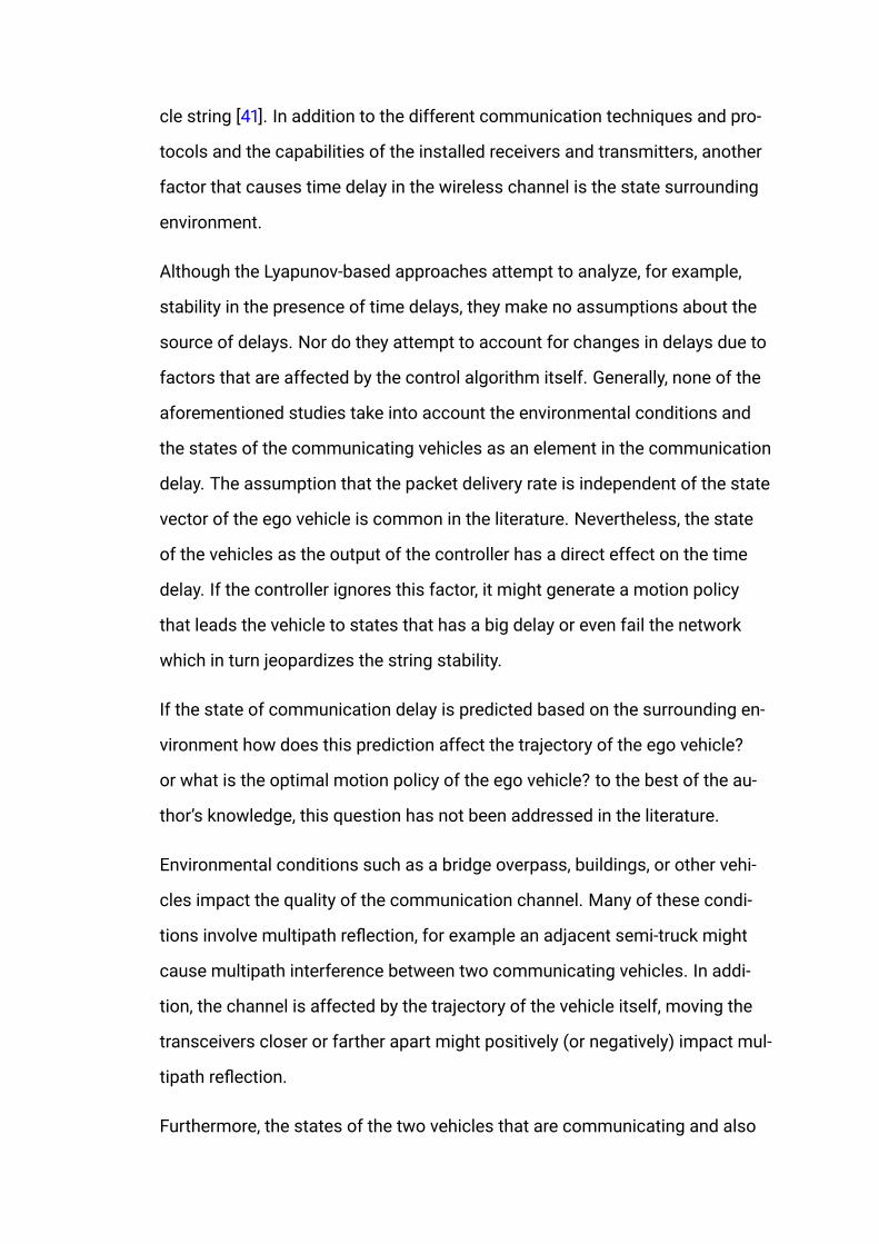
cle string [41]. In addition to the different communication techniques and pro-
tocols and the capabilities of the installed receivers and transmitters, another
factor that causes time delay in the wireless channel is the state surrounding
environment.
Although the Lyapunov-based approaches attempt to analyze, for example,
stability in the presence of time delays, they make no assumptions about the
source of delays. Nor do they attempt to account for changes in delays due to
factors that are affected by the control algorithm itself. Generally, none of the
aforementioned studies take into account the environmental conditions and
the states of the communicating vehicles as an element in the communication
delay. The assumption that the packet delivery rate is independent of the state
vector of the ego vehicle is common in the literature. Nevertheless, the state
of the vehicles as the output of the controller has a direct effect on the time
delay. If the controller ignores this factor, it might generate a motion policy
that leads the vehicle to states that has a big delay or even fail the network
which in turn jeopardizes the string stability.
If the state of communication delay is predicted based on the surrounding en-
vironment how does this prediction affect the trajectory of the ego vehicle?
or what is the optimal motion policy of the ego vehicle? to the best of the au-
thor’s knowledge, this question has not been addressed in the literature.
Environmental conditions such as a bridge overpass, buildings, or other vehi-
cles impact the quality of the communication channel. Many of these condi-
tions involve multipath reflection, for example an adjacent semi-truck might
cause multipath interference between two communicating vehicles. In addi-
tion, the channel is affected by the trajectory of the vehicle itself, moving the
transceivers closer or farther apart might positively (or negatively) impact mul-
tipath reflection.
Furthermore, the states of the two vehicles that are communicating and also

their relative position have significant effects on the quality of the channel [43].
Ignoring this fact might cause a vehicle to generate a motion policy that re-
sults in a communication loss or a low-quality communication channel, which
in turn impacts transferring information from vehicle to vehicle. Lack of in-
formation about the trajectory of, for example, a lead car of a platoon, forces
the following vehicle to generate a more conservative motion policy to satisfy
safety constraints with a worst-case assumption about the lead vehicle’s fu-
ture trajectory, i.e. forward invariance set. This implies that the states of the
vehicles and Packet Delivery Ratio (PDR) depend on each other and varia-
tions of one will impact the other. Accordingly, to have optimal performance,
it is necessary to involve both elements in a single controller algorithm at the
same time. But the challenge is, the nature of MPC and the model governing
PDR are different. The MPC is defined based on existing dynamical system of
the agent and desirable cost function and different constraints which all are
model-based. On the other hand PDR is a data-driven variable and to date an
explicit mathematical model does not exist to describe it.
2.4 Proposed Methods
This dissertation addresses the challenges that arise due to the interplay be-
tween model-based and data-driven components that are increasingly preva-
lent in various control tasks. To address these challenges, the dissertation
develops two approaches:
GP-MPC: that is a methodology to build a proxy model to predict the wireless
channel and merges it with model predictive control to find an optimal trajec-
tory that not only optimizes the conventional costs including fuel consump-
tion, comfort, safety and etc, but also takes a further step to minimize the PDR
to guarantee the stream of information in the time steps beyond the time hori-

zon.
Learning Model Predictive Control: an iterative learning control that involves
a data-driven variable in model predictive control to find an optimal trajectory
for both the model and data-driven systems. GP-MPC needs a reference trajec-
tory to follow, also it requires more training samples and running time. Another
downside of using GP is that, even if the system has linear dynamics, adding
an estimation of wireless channel to the cost function will make the model
non-convex. Such a result is not desirable in terms of running time and solu-
tion quality. This algorithm start form an initial trajectory which is assumed
to be available in the beginning and exploits the generated full trajectories to
generate a better one. This algorithm learns from its previous outputs and im-
proves them.
DMPC: that is a generic methodology for MPC to take into account a data-
driven variables in its decision-making. The preliminary version of this algo-
rithm in the last part, can take into account just a limited number of discrete
values of data-driven variable, and increasing the this number will make the
modeling process a demanding job. Therefore, we first develop DMPC to tackle
a continuously changing data-driven variables while keeping its advantages
over GP-MPC.

Chapter 3
Gaussian Process-based Model
Predictive Controller for CAVs
3.1 Introduction
In this chapter, a data-driven Model Predictive Controller is presented that
leverages a Gaussian Process to generate optimal motion policies for con-
nected autonomous vehicles in regions with uncertainty in the wireless chan-
nel. The communication channel between the vehicles of a platoon can be
easily influenced by numerous factors, e.g. the surrounding environment, and
the relative states of the connected vehicles, etc. In addition, the trajectories
of the vehicles depend significantly on the motion policies of the preceding ve-
hicle shared via the wireless channel and any delay can impact the safety and
optimality of its performance.
In the presented algorithm, Gaussian Process learns the wireless channel
model and is involved in the Model Predictive Controller to generate a control
sequence that not only minimizes the conventional motion costs, but also min-
imizes the estimated delay of the wireless channel in the future. This results in
a farsighted controller that maximizes the amount of transferred information

beyond the controller’s time horizon, which in turn guarantees the safety and
optimality of the generated trajectories in the future. To decrease computa-
tional cost, the algorithm utilizes the reachable set from the current state and
focuses on that region to minimize the size of the kernel matrix and related
calculations. In addition, an efficient recursive approach is presented to de-
crease the time complexity of developing the data-driven model and involving
it in Model Predictive Control. We demonstrate the capability of the presented
algorithm in a simulated scenario.
GPs have been used to model the dynamics of different systems, for instance
leveraging Gaussian Processes to model cart-pole system and a unicycle
robot [44] and inverted pendulum [45]. The same approach of [15] is used,
which is an improvement to Probabilistic Inference for Learning Control (PILCO)
methodology initially presented in [44] that has the ability to propagate uncer-
tainty through the time horizon of a predictive controller and learn the parame-
ters of a LTI system.
However, PILCO and its variants are computationally expensive, and in the con-
text of CAVs it is not critical to learn a LTI system. Another challenge with the
majority of learning algorithms is that they often require too many trials to
learn. For example, learning the mountain-car tasks often requires hundreds
or thousands of trials, independent of whether using policy or value iterations,
or policy search methods [46, 47]. Thus the reinforcement learning algorithms
have limited applicability to many real-world applications, e.g. mechanical sys-
tems, especially if their system dynamics change rapidly (such as wearing out
quickly in low-cost robots) [44].
To decrease the size of the learned GP model in MPC, the concept of N-step
reachable set (see section( 3.3.2) for details) is used to focus on a small part
of the model required to find the optimal motion policy from the current state.
Also, the repetitiveness of the MPC is exploited to develop a recursive ap-

proach to decrease the computational burden of the GP in MPC. Furthermore,
the veloped approach learns the parameters of a wireless channel and inte-
grates this information with known or explicit dynamical models. Therefore,
the contributions of this approach are
1. a computationally efficient controller that leverages and extends state-
of-the-art learning algorithms, and
2. a control architecture for CAVs that accounts for communication uncer-
tainty in a locally optimal way.
3.2 Background: MPC scheme for CAVs
Consider a platoon of autonomous vehicles that generate their own optimal
motion policy and share it with other vehicles in the platoon through a wireless
communication channel.
Given a leader-following pair of vehicles, let xt ∈ Rn and ut ∈ Rm be the state
and control vectors of the ego, or following, vehicle at time step t. Its dynami-
cal system is given by:
xt+1 = f (xt, ut) . (3.1)
It is assumed that f : Rn × Rm → Rn is a smooth function. The smoothness
of a function is a property measured by the number of continuous derivatives
it has over some domain. At the very minimum, a function could be consid-
ered smooth if it is differentiable everywhere (hence continuous). In this dis-
sertation, it is assumed that, the function f is at least twice differentiable. In
the following, the model predictive controller of the ego vehicle is presented,
first, under the condition of perfect communication channel and then imper-
fect communication channel.

3.2.1 Perfect Communication Channel
In this case it is assumed that there is no delay in the wireless channel and the
sent packet from the predecessor vehicle, that contains its predicted trajectory
for N time steps in the future, is being received by the ego vehicle at no time.
The controller of the ego vehicle for this case is proposed as an MPC architec-
ture that solves the following finite-horizon optimization model with length of
N at time t:
minutJ = Q(xt+N |t) +
t+N∑k=t
h(xk|t, uk|t) (3.2a)
s.t. xk+1|t = f(xk|t, uk|t
)(3.2b)
xt|t = xt (3.2c)
Φ(xk|t, xpk|t) ≥ ϕ (3.2d)
xk|t ∈ X , uk|t ∈ U ∀k ∈ t, . . . , t+N. (3.2e)
where h(xk|t, uk|t) is the stage cost and defined as:
h(xk|t, uk|t) = ‖xk|t − xpk|t‖2R1
+ ‖xk|t − xrefk ‖2R2
+ ‖uk|t‖2R3
(3.3)
and xk|t and uk|t are the state and control input vectors at step k predicted at
time t, respectively, which are shown as the solution of model (3.2):
xt =[xt+1|t, xt+2|t, ..., xt+N |t
]ut = [ut|t, ut+1|t, ..., ut+N−1|t].
(3.4)
The receding horizon control law applies the first control input ut|t of ut to shift
the state of the system to xt+1|t, and the process is repeated again from t + 1.
The cost function includes four terms to track: the state of predecessor ve-
hicle xpk|t, a desired reference trajectory xrefk , minimal control effort, and mini-

mum terminal cost Q. The tuning positive (semi)definite matrices are defined
by R1, R2, and R3. The optimal state vector of the lead vehicle, xpk|t, is sent via
the wireless channel in the following packet
xpt =[xpt+1|t, x
pt+2|t, ..., x
pt+N |t
]. (3.5)
The dynamical system and the initial condition are represented by (3.2b) and
(3.2c). Constraint (3.2d) enforces the safety conditions which can be defined
simply as a minimum euclidean distance or as the Time To Collision factor
that cannot be less than a given parameter ϕ
Φ(xk|t, xpk|t) =
∞ vpk|t ≥ vk|t
dk|tvk|t−v
pk|t
vpk|t < vk|t.
(3.6)
vk|t and dk|t are the velocity of the ego vehicle and its euclidean distance from
its predecessor at time step k predicted at time t. It is assumed that there is a
feasible trajectory from the initial state to the terminal state at time step t.
Equation 3.6 can be easily changed in standard form using a Boolean variable
αk|t ∈ 0, 1 and a big numberM as the following form:
Mαk|t +dk|t
vk|t − vpk|t(1− αk|t) ≥ ϕ (3.7a)
vk|t ≤ vpk|t +M(1− αk|t) (3.7b)
vk|t > vpk|t −Mαk|t (3.7c)
In this scheme (3.2), it is assumed that the communication channel is perfect
(common in literature, e.g. [35]), which means that the trajectory of the pre-
decessor vehicle xpk|t,∀k ∈ t, . . . , N + t is transferred without any delay to
the ego vehicle at the beginning of each time step, t. In this dissertation, this

assumption will be relaxed to capture the uncertainty of the wireless commu-
nication channel.
3.2.2 Imperfect Communication Channel
The communication channel can be impacted by numerous factors such as
relative states of the connected vehicles, surrounding infrastructure and vehi-
cles, free space disturbances, etc. The predicted state vector of the commu-
nication channel established between the ego vehicle and its predecessor is
defined as
wt = [wt+1|t, wt+2|t, . . . , wt+N |t]. (3.8)
wt+k|t shows the prediction for the packet delivery time of time step k + t be-
tween two vehicles calculated at time t (i.e. the inverse of packet delivery rate,
PDR).
The question that we address in this section is “How does predicted delivery
time affect the policy of the ego vehicle, and how can this delivery time be in-
volved in the optimization model of the controller?" If the estimated delivery
time wt+k|t is greater than the length of the time step used for the discretized
dynamics in the general MPC formulation, there will be an estimated delay at
time step t + k. In this case, the ego vehicle should use the most recent avail-
able packet, at time t+ k − 1, sent from the lead vehicle.
Due to the uncertainty in the delivery time of the packets, the ego vehicle can
receive several packets at a single time step, xpt1 , xpt2 , , ..., x
ptm, where t1 < t2 <
... < tm 6 t + k. Because the packet containing xptm is the most up-to-date
(though not necessarily current at time t + k), it is used to calculate the motion
policy of the ego vehicle.
xptm = [xptm|tm , xptm+1|tm , . . . , x
ptm+N |tm ]. (3.9)

Nevertheless, at time step t+ k, the first t+ k − tm states in this packet belong
to the past and are not useful anymore and should be neglected. Therefore,
the useful packet shrinks to:
xptm = [xpt+k|tm , xpt+1|tm , . . . , x
ptm+N |tm ]. (3.10)
The length of this packet determines the applicable time horizon in the model
predictive controller that the ego vehicle can consider to involve the trajectory
of the lead vehicle:
Nt+k = tm +N − (t+ k). (3.11)
where Nt+k denotes the length of time horizon at time t + k, Nt+k 6 N . In-
creases in the value of wt+k|t decreases tm, which in turn decreases the length
of the useful time horizon Nt+k. Fewer useful states from the lead vehicle
causes the ego vehicle to take more conservative policies to satisfy the safety
constraints, and this approach results in more cost for the entire whole tra-
jectory; i.e. the controller might find local optima due to lack of longer-term
information.
In this section, awareness of the cost is added to physical system performance
due to communication delays, which updates the cost function of model (3.2)
to:
minut
J = Q(xt+N |t) +t+N∑k=t
[h(xk|t, uk|t) + y(wk|t)], (3.12)
in which y is a positive definite function. Adding a notion of the packet delivery
time of the wireless channel to the cost function of the model equips the sys-
tem with a farsighted controller to guarantee the availability of the packet with
a maximum possible length at each time step in the future, ultimately resulting
in a safer and more optimal motion policy. Therefore, the objective function
includes the cost of the delay in communication channel for the trajectories
that result in a low quality state of communication channel, ωt+k|t. Thus, the

optimality condition forces the model to generate trajectories with desirable
quality of the communication while satisfying the constraints. In the next sec-
tion, the Gaussian Processes is used to estimate the state of wireless channel
at each time step, wk|t, as a function of the states of two connected vehicles.
3.3 Gaussian Process for CAVs
In this section, the main components of Gaussian Processes for connected
autonomous vehicles will be presented and it will be shown that how it is in-
volved in model predictive control. Later in the section, an efficient recursive
approach will be developed to improve the time complexity of the presented
algorithm.
3.3.1 Probabilistic Model for Wireless Channel
Assume that the delay of packet delivery from the lead vehicle to the ego vehi-
cle at time t can be described by the following unknown function
ωt = Ω(xt, xpt , e) + ε (3.13)
where e show the external environment and ε is noise ε ∼ N (0, σ2ε). In this
paper, a Gaussian Process setting is considered where deterministic control
inputs ut that minimize the expected long-term cost is sought.
minut
Jt→t+N +
t+N∑k=t
y(Eωk|t [ωk|t]). (3.14)
Jt→t+N denotes the conventional cost function in MPC, i.e. equation (3.2a),
and y(Eωk|t [ωk|t]) denotes the cost of expected delay in packet delivery at time

step k predicted at time t. To implement the GP the following augmented vec-
tor is used as training inputs:
x =
xxp
, x ∈ R2n (3.15)
In this vector, x and xp indicate the state of ego vehicle and the state of lead
vehicle associated with x, and ω ∈ R≥0 as training target. A GP as a probabilis-
tic, non-parametric model can be fully specified by a mean functionm(·) and
a covariance function k(·, ·) which is defined as squared exponential (Radial
Basis Function, RBF):
k(x, x′) = σ2Ωexp
(− 1
2(x− x′)TL−1(x− x′)
). (3.16)
where σ2Ω is signal variance, and L = diag([`2
1, . . . , `22n]) with length-scales
`1, . . . , `2n.
Assuming that there are r training inputs and corresponding training targets,
X = [x1, . . . , xr]T and ωωω = [ω1, . . . , ωr]T are collected. Given the test input de-
noted x∗, the posterior predictive distribution of ω∗ is Gaussian p(ω∗|x∗,X,ωωω) =
N(ω∗|m(x∗), σ2(x∗)
)where
m(ω∗) = k(X, x∗)T (K + σ2ε I)−1ωωω, (3.17)
σ2(ω∗) = k(x∗, x∗)− k(X, x∗)T (K + σ2ε I)−1k(X, x∗). (3.18)
K is the Gram matrix with entries of Ki,j = k(xi, xj) [48].
It is assumed that p(xk|t) = N (xk|t|µµµt,ΣΣΣt), where µµµk|t and ΣΣΣk|t are the mean
and covariance of xk|t. From equation (3.17), the cost function (3.14) can be

rewritten as
minut
Jt→t+N +t+N∑k=t
y(k(X, xk|t)T (K + σ2
ε I)−1ωωω), (3.19)
where xk|t is the aggregated vector including the state vectors of the ego and
lead vehicles. The first n elements of this vector (i.e. test input) in (3.15) be-
longs to the ego vehicle and will be decided by the model predictive controller
such that the overall cost takes a minimum value. The constraints (3.2b)-
(3.2e) hold for this cost function. After finding the best control input vector
ut, the first control action, ut|t, is applied and the state of the ego vehicle is up-
dated to xt+1|t.
3.3.2 Efficient Recursive GP-MPC
The GP-MPC algorithm needs to invert the Gram matrix, K, in cost function
(3.19), which has time complexity of O(r3), where r is the number of training
data. For large training sets (ten thousands or more) construction of GP re-
gression becomes an intractable problem. The time complexity of the algo-
rithm is improved in this section by leveraging the concept of Reachable Set to
decrease the size of matrix K.
Definition 1 (one-step reachable set B): For the system (3.1), the one-step
reachable set from the set B is denoted as
Reach(B) =x ∈ Rn : ∃x(0) ∈ B, ∃u(0) ∈ U , s.t. x = f(x(0), u(0))
(3.20)
Reach(B) is the set of states that can be reached in one time step from state
x(0). N -step reachable set are defined by iterating Reach(.) computations [49].
Definition 2 (N-step reachable setRN(X0)): For a given initial set X0 ⊆ X , the
N -step reachable setRN(X0) of the system (3.1) subject to constraints (3.2d)
and (3.2e) is defined as [49]:

Rt+1(X0) = Reach(Rt(X0)), R0(X0) = X0, t = 0, . . . , N − 1 (3.21)
To calculate the N−step reachable set from the initial state xt RN(xt), two
finite time optimal control problem can be built to determine the boundaries
for each desirable state. In this application, we are interested in states x and y.
The cost functions of this OCP is defined as minut minxt+k|t, ∀k, where all
the constraints hold. The optimal value for the cost function shows the lowest
value that is reachable in N time steps for state x. Similarly, another optimal
control problem with the cost function of minut −maxxt+k|t, ∀k is built to
find the maximum reachable value for state x. After finding the minimum and
maximum values for states x and y, the data-driven system is called to sample
from this limited range.
Using the N-step Reachable Set concept, sub-matrix K(t) is defined that is ex-
tracted from matrix K
Ki,j(t) = k(xi, xj)|xi, xj ∈ RN(xt) ∩ X. (3.22)
This will result in the following cost function
minut
Jt→t+N +t+N∑k=t
y(k(Xt, xk|t)T (K(t) + σ2
ε I)−1ωωωt), (3.23)
where Xt = x|x ∈ RN(xt) ∩ X and ωωωt is the associated training output. As-
sume that the sampling has been executed randomly and for each time step, ν
samples are available on average. The number of training data extracted from
the overall training data, X, would be νN , where νN r. Constructing the
sub-matrix K(t) is straightforward and can be implemented based on the state

vector of lead vehicle, xp, and the defined safety constraint (3.2d).
Lemma 1. Given Matrix K(t−1) denoting the sub-matrix extracted from matrix K
and containing N-step Reachable Set at time step t−1, and its inverse K−1(t−1),
then K−1(t) can be calculated in O(ν3N2) time.
Proof. In the given matrix K(t − 1), ν training data representing the wireless
channel at time step t − 1 should be removed because the controller has im-
plemented one step of control input, ut|t. In addition, training data representing
time step t + N that is obtained fromRN(xt) should be added to the matrix.
The result of these two steps will be matrix K(t). According to the approach, ν
training data will be removed and added, which keep the size of matrix K−1(t)
the same, νN .
The Sherman–Morrison formula [50] is used to find K−11,1(t − 1) (i.e. matrix
K−1(t− 1) that its first column and row are removed) from K−1
(t− 1). Based on
this formula
K−11,1(t− 1) =
(K(t− 1)− pqT
)−1
1,1. (3.24)
where p and q are defined as: p = K1(t − 1) − e1, and q = e1, (ei is ith canonical
column vector). The right hand side of equation (3.24) can be expanded as:
(K(t− 1)− pqT
)−1
1,1= K−1
(t− 1) +K−1
(t− 1)pqT K−1(t− 1)
1− qT K−1(t− 1)p
. (3.25)
1 − qT K−1(t − 1)p is assumed to be invertible. This term can be calculated in
O(ν2N2), which comes from multiplication of the square matrix K−1(t− 1) with
dimension (νN × νN) and vector p and qT . We denote the new training set as
X′t−1, that has one less training data than Xt−1.
In the second step, a new training data, x, is added.

M :=
K1,1(t− 1) k(X′t−1, x)
k(X′t−1, x)T k(x, x)
(3.26)
Now, given K−11,1(t− 1), we can find the inverse of matrixM by using Schur com-
plement [51]. The Schur’s complement of K1,1(t− 1) in matrixM is given by:
M/K1,1(t− 1) := k(x, x)− k(X′t−1, x)T K−11,1(t− 1)k(X′t−1, x) (3.27)
Assuming thatM/K1,1(t − 1) is invertable,M−1 can be calculated in O(ν2N2)
as:
M−12,2 = (M/K1,1(t− 1))−1 (3.28)
M−12,1 = −M−1
2,2k(X′t−1, x)T K−11,1(t− 1)
M−11,2 = −K−1
1,1(t− 1)k(X′t−1, x)M−12,2
M−11,1 = K−1
1,1(t− 1)−M−11,2k(X′t−1, x)T K−1
1,1(t− 1). (3.29)
Removing and adding a row and a column both are calculated in O(ν2N2).
These two steps should be repeated for ν times, which yields to time complex-
ity of O(ν3N2).
Details of the algorithm are presented in Algorithm (1).
3.4 Example Scenario - Uncertain Communication Channel
In this chapter, GP-MPC method is applied on two connected vehicles and it
is assume that there is a region where the packet delivery rate is impacted
significantly; this region is unknown a priori by the controller. The expected
packet delivery time of the wireless channel between two connected vehi-
cles is demonstrated by contour plot in Figure (3.1). Wireless channel model

Algorithm 1 : Calculating K−1(t) from K−1
(t− 1)
1: load training data X, K(t− 1) and K−1(t− 1)
2: Xt ← RN(xt) ∩ X3: X′t−1 ← Xt−1
4: calculate K(t), equation (3.22)5: E ← K(t− 1), E−1 ← K−1
(t− 1)6: for all i = 1 : ν do7: p← E − e1, and q = e1
8: E−11,1← (E − pqT )−1
1,1, equations (3.24),( 3.25)
9: X′t−1 ← X′t−1 − X′t−1110: load new training data x from X
11: E ←[
E1,1 k(X′t−1, x)
k(X′t−1, x)T k(x, x)
]12: calculate k(X′t−1, x) and k(x, x)
13: S ← k(x, x)− k(X′t−1, x)TE−11,1k(X′t−1, x), equation (3.27)
14: M−12,2 ← S−1
15: M−12,1 ← −M−1
2,2k(X′t−1, x)TE−11,1
16: M−11,2 ← −E−1
1,1k(X′t−1, x)M−1
2,2
17: M−11,1 ← E−1
1,1−M−1
1,2k(X′t−1, x)TE−11,1
18: E−1 ←[M−1
1,1 M−11,2
M−12,1 M−1
2,2
]19: X′t−1 ← X′t−1 ∪ x20: end for21: K−1
(t)← E−1
22: K(t)← E23: Xt ← X′t−1

is learned by Gaussian Processes and according to Algorithm (1) in section
(3.3.2). After obtaining the necessary training input for state xt, Xt, the inverse
of associated kernel matrix K−1(t) is calculated according to Lemma (1). Fi-
nally, the cost function (3.23) is built, and the GP-MPC proceeds by solving a
sequential quadratic program.
In the following example scenario,
In this leader-follower scenario, the vehicles dynamics are formulated as a Lin-
ear Time Invariant (LTI) system xt+1 = Axt+But, ∀t, where xt = [xt xt]T , ut = xt
and
A =
1 dt
0 1
and B =
dt22
dt
. (3.30)
The system is subject to input saturation and it is assumed that the lead ve-
hicle has a constant velocity 5m/s and the ego vehicle should keep the safe
distance of at least ϕ = 2m form the lead vehicle, Φ(xk|t, xpk|t) ≥ 2, which is en-
forced by constraint (3.2d). The time horizon is considered to be N = 10 and
the length of each time step is dt = 1s. The upper and lower bound values of
the state and input values are xt ∈ [3, 10] and xt ∈ [−3, 2].
The trajectory of the lead vehicle is depicted by a red line in Figure (3.1), and
a controller is developed that finds an optimal trajectory for the ego vehicle
that not only minimizes the conventional motion cost, but also minimizes
the expected delay time in the packet delivery (recalling again that the con-
troller knows nothing about the contours in Figure (3.1) in advance). The blue
line shows the optimal trajectory generated by GP-MPC for the ego vehicle.
It can be seen from the second Figure (3.2) that, to maintain adequate wire-
less channel status (and to optimally balance control cost, safety, wireless
performance, and do this as fast as possible), the ego vehicle decelerates
to increases its distance from the lead vehicle. This policy sacrifices a bit of
short-term performance in order to maintain connectivity, improving situa-

Figure 3.1: Optimal trajectory of ego vehicle generated by GP-MPC to avoid aregion with a considerable delay time in packet delivery.
tional awareness and ultimately long-term performance.
3.5 Conclusions
In this chapter, an efficient Model Predictive Control algorithm based on Gaus-
sian Processes is presented to account for uncertainty in the communication
channel of motion policies in connected vehicle applications. The presented
algorithm learns the wireless channel model in terms of expected packet deliv-
ery time by leveraging Gaussian Processes. Due to the substantial amount of
available training data, the obtained GP model is very large and computation-
ally expensive to deal with.
To solve this problem, the algorithm focuses on the N-step reachable set from
the current state of the ego vehicle as the useful training data set. This de-
creases the size of the required training data for the current state of the vehi-
cle dramatically. Subsequently the resultant kernel matrix would be substan-

Figure 3.2: Optimal control input xt, state xt and inter-vehicular distance dtover the time horizon.
tially smaller than the original Gram matrix, which needs less computational
effort to be inverted and multiplied. In addition, because a major part of the
computation involved in GP is conducted to find the inverse of the kernel ma-
trix, the controller exploits the recently calculated and readily available inverse
of the kernel matrix from the previous state. The Sherman-Morrison formula
and Schur complement were used to find the inverse of the current kernel ma-
trix after updating the training data set. These steps decrease the running time
to find the expected packet delivery time of the wireless channel for the given
time horizon N from O(r3) to O(ν3N2) where r and ν are the number of overall
training data and drawn data for a single time step, respectively, and νN r.
To demonstrate the approach, a simulation of a leader-follower scenario for
two connected autonomous vehicles is developed and the results of the algo-
rithm presented.
Chapter 4
Learning Model Predictive Control
for CAVs
In chapter (3), GP-MPC algorithm was developed to address the problem of
involving the variations of wireless channel as a proxy model of states of two
communicating vehicles and surrounding environment into the conventional
model predictive control setting. The presented technique works, but there are
few disadvantages in this approach:
• In the case of controlling a linear system, GP will transform the prob-
lem to a nonlinear optimal control model, which is a negative point for
GPMPC.
• GPMPC needs lots of data to create a proxy model for the unknown model
and providing a big state space will make GP intractable to handle. This
problem was partially overcome by by developing a recursive approach
to calculate the kernel matrix and confining the state space by the con-
cept of N-step reachable set, but it still demands lots of effort.
• It is not easy to study the asymptotic stability of the equilibrium point
and feasibility of the trajectory from the initial state to the terminal state,

beyond the time horizon.
• GP-MPC, similar to MPC, is unable to observe the state space beyond the
time horizon. This causes a local optimal trajectory in MPC (and in some
cases infeasible trajectory), because the controller assumes a euclidean
cost that is a naive alternative for cost from the state of the end of time
horizon, xt+N |t, and the terminal state, xF .
In this chapter, Learning Model Predictive Controller (LMPC) [52] is presented
and tailored to Connected Autonomous Vehicles (CAVs) applications. This
algorithm is developed for the wireless channel with a limited number of dis-
cretized PDR values. This assumption will be removed in the next chapter. The
proposed controller builds on previous work on nonlinear LMPC, adapting its
architecture and extending its capability to account for data-driven decision
variables that derive from an unknown or unknowable function. The chapter
presents the control design approach, and shows how to recursively construct
an outer loop candidate trajectory and an inner iterative LMPC controller that
converges to an optimal strategy over both model-driven and data-driven vari-
ables. Simulation results show the effectiveness of the proposed control logic.
In this chapter, recent advances in data-driven MPC [52–54] are leveraged
that learn from previous iterations of a control task and provide guarantees on
safety and improved performance at each iteration. In particular, a formulation
of MPC for vehicle platooning is introduced that accounts for imperfect com-
munication, and then a LMPC control scheme is designed that leverages the
notion of predictive capability for wireless channel quality, in order to obtain
better platoon performance. The contributions of this chapter are:
1. formulation of a (L)MPC problem that can handle decision variables or
objective functions that derive from an unknown or unknowable function,
for example variables that are generated by an artificial neural net, and
2. extension of LMPC, adapted to handle dynamic environments and/or
time-evolving constraints, in a computationally tractable manner.
In this chapter, finding a solution for the following infinite time optimal control
problem is of interest:
minuJ(xS) =
∞∑k=0
h(xk, uk) (4.1a)
s.t. xk+1 = f (xk, uk) , ∀k ≥ 0 (4.1b)
x0 = xS (4.1c)
Φ(xk, x`k) ≥ ϕ, ∀k ≥ 0 (4.1d)
xk ∈ X , uk ∈ U , ∀k ≥ 0. (4.1e)
4.1 Preliminaries of Learning Model Predictive Control
This section is based on the original work of [52]. Beginning with a discrete
time system
xt+1 = f (xt, ut) , (4.2)
where x ∈ Rn and u ∈ Rm are the system state and input, respectively, as-
sume that f(·, ·) is continuous and that state and inputs are subject to the con-
straints
xt ∈ X , ut ∈ U , ∀t ≥ 0, (4.3)
LMPC solves the following infinite horizon optimal control problem iteratively:
J∗0→∞ = minu0,u1,...
∞∑k=0
h (xk, uk) (4.4)
s.t. xt+1 = f (xt, ut) ∀k ≥ 0 (4.4a)
x0 = xS (4.4b)
xk ∈ X , uk ∈ U ∀k ≥ 0 (4.4c)

where equations (4.4a) and (4.4b) represent the system dynamics and the ini-
tial condition, and (4.4c) are the state and input constraints. LMPC assumes
that the stage cost h(·, ·) in equation (4.4) is continuous and satisfies
h (xF , 0) = 0 and h(xjt , u
jt
) 0 ∀xjt ∈ Rn \ xF , ujt ∈ Rm \ 0 (4.5)
where the final state xF is a feasible equilibrium for the unforced system (4.2)
f(xF , 0) = xF .
At the jth iteration of LMPC, the vectors
uj =[uj0, u
j1, . . . , u
jt , . . .
](4.6a)
xj =[xj0, x
j1, . . . , x
jt , . . .
](4.6b)
collect the inputs applied to system (4.2) and the corresponding state evolu-
tion. In (4.6), xjt and ujt denote the system state and the control input at time t
of the jth iteration. It is assumed that at each jth iteration, the closed loop tra-
jectories start from the same initial state
xj0 = xS, ∀j ≥ 0. (4.7)
4.1.1 Sampled Safe Set
A key notion of LMPC is that it exploits the iterative nature of control design.
For every kth iteration that successfully steers the system to the terminal point
xF (i.e.,∀k : limt→∞ xkt = xF ), the trajectory xk is a subset of sampled Safe Set
Sj , which is defined as:
Sj =
⋃i∈Mj
∞⋃t=0
xit
(4.8)

where
M j =k ∈ [0, j] : lim
t→∞xkt = xF
(4.9)
Sj is the collection of all state trajectories at iteration i for i ∈ M j . M j in (4.9)
is the set of indices k associated with successful iterations of MPC for k < j.
It follows that S i ⊆ Sj ∀i ≤ j. Sj is a subset of the maximal stabilizable set
because, for every point in the set, there exists a feasible control action that
satisfies the state constraints and steers the state toward xF .
4.1.2 Iteration Cost
Function Qj(·) is defined over Sj that assigns to every point in Sj the minimum
cost-to-go along the trajectories in sampled safe set,
Qj(x) =
min
(i,t)∈F j(x)J it→∞(x), if x ∈ Sj
+∞ if x /∈ Sj(4.10)
where F j(·) is
F j(x) =
(i, t) : i ∈ [0, j], t ≥ 0 with xit = x; ∀xit ∈ Sj (4.11)
In other words, for every x ∈ Sj , Qj(x) not only assigns the optimal cost-to-go
but also the pair (i, t) that indicates the optimal iteration number in LMPC as
well as the optimal time-to-go for that state.
4.1.3 LMPC Formulation
LMPC tries to find a solution for the infinite time optimal control problem (4.4)
by solving the following constrained finite time optimal control problem at

each time step, t of iteration j:
Jt→t+N(xjt) = minut|t,...,ut+N−1|t
t+N−1∑k=t
h(xk|t, uk|t
)+Qj−1(xt+N |t) (4.12)
s.t. xk+1|t = f(xk|t, uk|t
)∀k ∈ t, . . . , t+N − 1 (4.12a)
xt+N |t ∈ Sj−1 (4.12b)
xt|t = xjt (4.12c)
xk|t ∈ X , uk|t ∈ U ∀k ∈ t, . . . , t+N − 1 (4.12d)
where (4.12a) and (4.12c) represent the dynamics of the system and initial
condition, respectively. The feasibility conditions on state and control vectors
are imposed by (4.12d). The constraint (4.12b) forces the controller to select
the terminal state from the safe set Sj−1. The optimal solution for this model
are shown as:
xjt:t+N |t = [x∗,jt , . . . , xjt+N |t] (4.13a)
ujt:t+N |t = [ujt|t, . . . , ujt+N−1|t]. (4.13b)
Being MPC, the first control input from vector ujt:t+N |t is applied to the system:
u∗,jt = ujt|t, x∗,jt+1 = xjt+1|t. (4.14)
Again, the finite time optimal control problem 4.12 is solved at time step t +
1 using the newly update state x∗,jt+1 and so on. This process of iteration will
result in a moving or receding horizon control strategy.
Assumption 1: At the first iteration, it is assumed that S0 is non-empty set, and
the provided trajectory from the initial state to the terminal state is feasible
and convergent to the terminal state.
This assumption is not restrictive in practice and can be generated easily in

different applications. Sequences of finite time optimal control model can
be used to drive the system from the initial state to the terminal state by ran-
domly selecting a number of final states for each of these models. For exam-
ple, in an autonomous vehicle case, the car can be run by following a reference
path in a very low speed to obtain a feasible sequence of states and control
inputs.
It can be shown [52] that, using the above notions of sampled safe set and
iteration cost, the jth iteration cost is nonincreasing at each iteration and that
the LMPC formulation is recursively feasible (state and input constraints at the
next iteration are satisfied they are satisfied at the current iteration).
4.2 Learning Model Predictive Control for CAVs
The original LMPC formulation presented above is designed for an entire tra-
jectory from an initial state to a final state, in a static environment. As those
authors acknowledge, LMPC is computationally expensive; in addition, LMPC
cannot be applied in a dynamic environment in its original form. To overcome
these limitations, we propose two concepts. The first notion involves encoding
the dynamics of obstacles both in the constraints and the objective function
of the optimization problem. In addition, LMPC is reformulated from an end-to-
end planning problem (i.e. find an optimal trajectory from xS → xF ), which typi-
cally has better performance in terms of the number of required iterations and
degree of optimality, as the planning horizon, N , increases [55]. In a dynamic
context, a shorter planning horizon trades convergence to global optima with
the ability to overcome computational issues with LMPC in general.
In addition, LMPC is extended to account for decision variables with unknown
dynamics or data-driven approximations. The control architecture includes
a (nominal) outer loop, or high level, motion planner that generates a candi-

date set of feasible trajectories. LMPC works on the inner loop to converge to
a feasible trajectory with optimal (or improved) performance over data-driven
decision variables.
The presented approach assumes the existence of a feasible trajectory from
the current state of the ego vehicle (i.e. the follower), xt → xt+N at the first
iteration but with no assumptions on optimality, given as
x0t = [x0
t|t, x0t+1|t, . . . , x
0t+N |t] (4.15a)
u0t = [u0
t|t, u0t+1|t, . . . , u
0t+N−1|t] (4.15b)
where x0k|t and u0
k|t are the state and control input vectors of the ego system
at time k that have been calculated at time step t. The superscript shows the
iteration number of LMPC, which starts from 0 and is denoted by index j ∈
0, 1, . . . . The presented algorithm keeps only a record of successful iter-
ations in this set. The information of each trajectory is saved in set S if it is
completed successfully, which implies no collisions but not necessarily opti-
mality. Given an arbitrary, feasible initial trajectory stored in S0, the dynamic
safe set is iteratively built as
Sj =
N⋃k=1
xjt+k|t
∣∣∣ xjk ∈ X , ujk ∈ U , ∀k ∈ t, t+ 1, . . . , t+N
∪ Sj−1 (4.16)
where x ∈ X includes the dynamic constraints on state imposed by the time-
to-collision for the predicted leader trajectory at time t.
The cost-to-go of state xk|t is denoted by q(xk|t|x`∗k→N |t) and is defined as “the
trajectory cost of the ego system from x(k|t) to x(k+N |t) given that the states
of the leading vehicle are [x`∗k|t, ..., x`∗N |t]". A backward calculation is applied to
find the cost-to-go for each state in set Sj . To start, qj(xjN |t|x`∗N |t) can be ap-
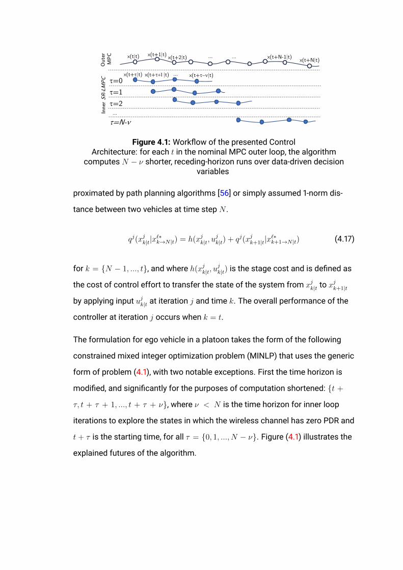
x(t|t) x(t+1|t)x(t+N|t)x(t+N-1|t)
x(t+t|t) x(t+t-n|t)x(t+t+1|t)
…
…t=0t=1t=2
t=N-n…
…
Out
er
MPC
Inne
r SR
-LM
PC
x(t+2|t)
Figure 4.1: Workflow of the presented ControlArchitecture: for each t in the nominal MPC outer loop, the algorithm
computes N − ν shorter, receding-horizon runs over data-driven decisionvariables
proximated by path planning algorithms [56] or simply assumed 1-norm dis-
tance between two vehicles at time step N .
qj(xjk|t|x`∗k→N |t) = h(xjk|t, u
jk|t) + qj(xjk+1|t|x
`∗k+1→N |t) (4.17)
for k = N − 1, ..., t, and where h(xjk|t, ujk|t) is the stage cost and is defined as
the cost of control effort to transfer the state of the system from xjk|t to xjk+1|t
by applying input ujk|t at iteration j and time k. The overall performance of the
controller at iteration j occurs when k = t.
The formulation for ego vehicle in a platoon takes the form of the following
constrained mixed integer optimization problem (MINLP) that uses the generic
form of problem (4.1), with two notable exceptions. First the time horizon is
modified, and significantly for the purposes of computation shortened: t +
τ, t + τ + 1, ..., t + τ + ν, where ν < N is the time horizon for inner loop
iterations to explore the states in which the wireless channel has zero PDR and
t + τ is the starting time, for all τ = 0, 1, ..., N − ν. Figure (4.1) illustrates the
explained futures of the algorithm.

The objective function is modified to
J jt+τ→t+τ+ν(xjt+τ ) =
t+τ+ν−1∑k=t+τ
‖xk+1|t − x`∗k+1|t‖2P1
+ ‖uk+1|t‖2P2
+
j−1∑i=0
N∑r=0
zirqi(xit+r|t|x`∗t+r→N |t) (4.18)
All of the constraints (4.1b)-(4.1e) hold, given appropriate sets k ∈ t+τ, . . . , t+
τ − ν.
Finally, to force the controller to select the final state from the safe set the fol-
lowing constraints are added:
xt+τ+ν|t =
j−1∑i=0
N∑r=0
zirxit+r|t (4.19a)
j−1∑i=0
N∑r=0
zir = 1 (4.19b)
zir ∈ 0, 1,∀i = 0, .., j − 1, ∀r = 0, ..., N (4.19c)
The following vectors show the optimal solution for this model:
Xt+τ = [xt+τ+1, xt+τ+2, ..., xt+τ+ν ]
Ut+τ = [ut+τ , ut+τ+1, ..., ut+τ+ν−1]
(4.20)
This model assigns a binary decision variable, zir , to each of the states in Sj
(4.16) and selects one of them as the terminal state, (4.19a). Because only
one of these states can be chosen as the terminal state xt+N |t, the summa-
tion of the binary variables should be exactly one, as shown in (4.19b). The last
term of the objective function (4.18) determines the best value for cost-to-go
qj(xjt+r|t|x`∗t+r→N |t) and its associated state. Assuming that the optimal state in
set Sj is xi∗t+r∗|t, the solution for system state is the vector
xt+τ+ν = xi∗
t+r∗|t (4.21)

After finding the optimal solution as an MINLP model, the first step of the con-
trol input vector, Ut+τ , is implemented and the related state and control vectors
are saved in the trajectory of iteration j:
xjt+τ+1|t = xt+τ+1
ujt+τ |t = ut+τ(4.22)
The updated trajectory in the current iteration, j, is as follows (notice the slightly
different symbol for x and u, indicating the first step of the receding horizon
LMPC along the time-shift τ ):
xjt = [xjt+1|t, xjt+2|t, . . . , x
jt+τ+1|t]
ujt = [ujt|t, ujt+1|t, . . . , u
jt+τ |t] (4.23)
for τ = 0, 1, ..., N − ν.
Similar to the previous chapter, it is assumed that given a trajectory, there is
a data-driven system that is able to predict the packet delivery rate for each
states.
ωωωjt+τ :t+τ+ν|t = [ωjt+τ |t, ωjt+τ+1|t, . . . , ω
jt+τ+ν|t] (4.24)
This information should be merged into the learning model predictive control.
The updated formulation should include communication delay, ωωωjt+τ , in the ob-
jective function to penalize the trajectory that results in low quality (predicted)
communication channel. To recognize the part of state space with low qual-
ity PDR, the vector should be utilized to update an obstacles area that repre-
sents the wireless channel. And, if the controller selects a state from this area,
it will be penalized in the cost function. Thus, the optimality condition forces
the model to generate a trajectory in which the quality of the communication
achieves an acceptable level, to avoid extra cost in the objective while satisfy-
ing the constraints.

To solve this problem, the repetitive nature of LMPC is exploited to consider
the variation of PDR as a data-driven factor in the optimization process. This
is done by two modifications in the model. First, qj is updated in the objec-
tive function to include the cost associated with the delay in the communica-
tion channel if a specific terminal state is chosen. Observe that the cost-to-go
vector is updated after a complete trajectory is generated. Second, a dynamic
constraint is added to the model to represent the area where the communica-
tion loss occurs and is updated at each inner loop iteration. For the first part,
the cost-to-go in the objective function is reformulated as:
qj(xjk|t|x`∗k→N |t) =
t+N∑p=k
[ωjp|t + h(xjp|t, u
jp|t)]
= h(xjk|t, ujk|t) + ω(xjk|t|x
`∗k|t) +
t+N∑p=k+1
ωjp|t + qj(xjk+1|t|x`∗k+1→N |t)
The updated cost-to-go contains the cost of delivery time of communication
channel and by replacing it in the objective function, the model will chose a
terminal state that has lower cost in terms of communication channel, and
stage costs.For the second part, a boundary on the state vector is defined as a
dynamic constraint in the model and is updated iteratively based on the vector
of packet delivery time received from data driven system. An auxiliary binary
decision variable is defined to distinguish the states selected from O
βk =
0 xjk|t /∈ O
1 xjk|t ∈ O(4.25)
If O is a polyhedron in Rn
O = xjk|t ∈ Rn : Axjk|t 6 b (4.26)
where A ∈ Rn×d and b ∈ Rd, the following set of inequalities determine if the

state is inside of O to assign an appropriate value to the binary variable βk,m
aTmxjk|t +Mβk,m > bm (4.27a)
aTmxjk|t −M(1− βk,m) < bm (4.27b)
βk,m ∈ 0, 1,∀m = 1, .., d (4.27c)
whereM is a large number. If∑d
m=1 βk,m = d, the state xjk|t is inside of O and
should be penalized in the cost function. Therefore, another binary variable is
defined
λk =
0∑d
m=1 βk,m < p
1∑d
m=1 βk,m = p
(4.28)
Using λk as auxiliary variables, the described cost term can be added to the
objective functiont+τ+ν∑k=t+τ+1
λkCk (4.29)
Vector Ck shows penalty that is added to the objective function if the con-
troller selects state xjk|t inside of the area. The following inequalities control
the value of λk
∑dm=1 βk,m −Mλk < p (4.30a)∑dm=1 βk,m +M(1− λk) > p (4.30b)
λk ∈ 0, 1 (4.30c)
A scenario of two connected vehicles is developed and an area is added where
the communication is impacted by the surrounding environment. However,
there are different applications in which the uncertainty of the network state
is involved to generate an optimal motion policy for the vehicles, for instance
autonomous intersection control [26, 27], where the vehicles approaching to
the intersection receive information from a central machine that manages it.

In the simulation, it is assumed that if both vehicles enter the so-called "dead-
zone" (i.e. plotted in time-location graph) the communication is completely
lost and the wireless channel is perfect out of this area. Also, we assume that
these characteristics can be recognized by a network state predictor given the
states of two vehicles over the planning time. Note that, the controller does
not have access to this information and the controller should be able to opti-
mize its motion policy without any knowledge about driving closed-form func-
tion of the state of channel ( i.e. described as a data-driven decision variable)
in either the objective or constraints and by receiving its prediction from an
exogenous system.
In this leader-follower scenario, the vehicles dynamics are formulated as a Lin-
ear Time Invariant (LTI) system xt+1 = Axt+But, ∀t, where xt = [xt xt]T , ut = xt
and
A =
1 dt
0 1
and B =
dt22
dt
. (4.31)
The system is subject to input saturation and the leader has a constant veloc-
ity of 30m/s over the planning time and the ego vehicle has an initial velocity
of 35m/s and its controller is limited to safety constraints. For other parame-
ters see Table (4.1).
Table 4.1: Scenario and Model Parameters
u,u control input limits m/s2 [-6,6]N time horizon of outer loop MP – 100ν time horizon of inner loop – 60dt sample time or discretization s 0.2vss` lead vehicle speed (constant) m/s 30vf,0 follower vehicle initial speed m/s 35Ωd dropout zone of bridge m 392-551
First, to show the improvement in the performance of the algorithm, the ma-
trix coefficient of the entering to the deadzone is considered a big value to
prevent the controller from generating a motion policy crossing over the red

Figure 4.2: Car-following scenario: The ego vehicle should avoid thedead-zone region (red rectangle)
region. Figure (4.2) illustrates the results of this case. The total number of at-
tempts required for the algorithm to converge to the optimal trajectory is 3
iterations. The top-left graph shows the cost-to-go vector for each of the tra-
jectories, which the severe decrease in the first two trajectories depict the cost
of deadzone. Also, the down-right one is the overall cost-to-go value for each
iterations which is a decreasing graph and converges from the initial trajectory
to the better one at each generation.
Without the ability to predict communication performance, the ego vehicle
tries to optimize on following distance and terminal cost. But, once it enters
the dead zone, it starts to drop packets and can only use increasingly shorter
portions of (previously communicated) leader trajectory predictions. In the
case of using the presented algorithm with communication prediction, the
controller has access to the prediction of the channel which tells whether the
channel is expected to change in the future. The algorithm is able to converge
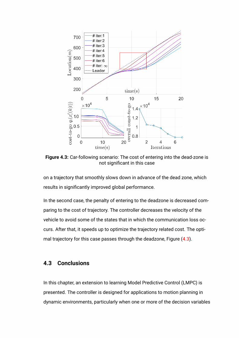
Figure 4.3: Car-following scenario: The cost of entering into the dead-zone isnot significant in this case
on a trajectory that smoothly slows down in advance of the dead zone, which
results in significantly improved global performance.
In the second case, the penalty of entering to the deadzone is decreased com-
paring to the cost of trajectory. The controller decreases the velocity of the
vehicle to avoid some of the states that in which the communication loss oc-
curs. After that, it speeds up to optimize the trajectory related cost. The opti-
mal trajectory for this case passes through the deadzone, Figure (4.3).
4.3 Conclusions
In this chapter, an extension to learning Model Predictive Control (LMPC) is
presented. The controller is designed for applications to motion planning in
dynamic environments, particularly when one or more of the decision variables

comes from black box or data-driven models. The control architecture lever-
ages a nominal outer loop motion planner, and then iterates over this trajec-
tory candidate in an inner loop to find optimal policies in terms of both model-
and data-driven variables. This outer and inner control scheme proceeds in a
receding horizon fashion until the system reaches its objectives. These con-
cepts are applied to connected autonomous vehicles and the notion of pla-
tooning, or collaborative adaptive cruise control.
To demonstrate the approach, a simulation of a leader-follower scenario for
two connected autonomous vehicles is developed. The scenario includes
physical characteristics that cause uncertainty in the communication channel,
and the controller leverages recent advances in wireless channel prediction
using machine learning. The presented algorithm is able to generate improved
trajectories in terms of not only communication, but also energy efficiency.

Chapter 5
Data-and Model-Driven Approach to
Predictive Control
5.1 Introduction
In the previous chapter a learning model predictive control approach was pre-
sented to involve the variations of wireless channel in the model predictive
control of an autonomous vehicle. The algorithm could recognize the area
with imperfect communication channel and based on the cost coefficients
of cost function, the controller was taking effective strategy to avoid the area.
But the idea of involving a soft constraint in the optimal control to build the
area representing the behavior of the wireless channel is demanding and is
limited to discretized values of PDR. PDR is a continuous parameter and an
effective algorithm is required to relax this limitation.
This chapter presents DMPC (Data-and Model-Driven Predictive Control) to
solve an MPC problem that deals with an unknown function operating interde-
pendently with the model. The value of the unknown function is predicted for
a given trajectory by an exogenous data-driven system that works separately
from controller. DMPC is a learning controller that provides an approach to

merge both the model-based (MPC) and data-based systems. This algorithm
can cope with very little data and builds its solutions based on the recently
generated trajectory and improves its cost in each iteration until converging to
an optimal trajectory, which typically needs only a few trials. Theoretical anal-
ysis for recursive feasibility of the algorithm is presented and it is proved that
the quality of the trajectory does not get worse with each new iteration. In the
end, we apply DMPC algorithm on motion planning of an autonomous vehicle
with linear and nonlinear dynamics and illustrate its performance.
Traditional techniques for analyzing and developing control laws in safety-
critical applications usually require a precise mathematical model of the sys-
tem [2–4]. However, there are many control applications where such precise,
analytical models can not be derived or are not readily available. Increasingly,
data-driven approaches from machine learning are used in conjunction with
sensor or simulation data in order to address these cases. Such approaches
can be used to identify unmodeled dynamics in a scalable way, and with high
accuracy. However, an objective that is increasingly prevalent in the literature
involves merging or complementing the analytical approaches from control
theory with techniques from machine learning.
Developments in model predictive control (MPC) and reinforcement learning
are most relevant to the techniques developed in this chapter. Recently, tech-
niques based on model predictive control (MPC) have addressed this problem
by first using a statistical method to estimate a mathematical model that is
compatible with the data, and then using this estimated model within a nom-
inal MPC framework to find optimal trajectories and control actions. A pop-
ular choice is to build statistical models using Gaussian Processes (GPs)
[48, 57, 58], while Regression Trees and other machine learning techniques
have been used in other cases [59,60]. The use of GPs in context of model pre-
dictive control often creates highly nonlinear models, resulting in non-convex

problems that are difficult to solve efficiently or online.
Alternatively, approaches based on Reinforcement Learning have been applied
in this setting. Model-based techniques again require a statistical technique,
for example GPs or deep neural networks, to estimate transition probability
distributions [61,62]. Model-free methods represent, informally, a trial-and-error
method for identifying control policies [15, 44]. An open question in reinforce-
ment learning (and indeed much of the literature that uses both controls and
machine learning) involves how to guarantee that the learned policy will not
violate safety or other constraints. In addition, sample complexity represents
a challenge for all the aforementioned techniques and is a general problem in
machine learning.
This chapter seeks to leverage the notion that in many applications, some as-
pects of the system (and environment) may be known mathematically while
other aspects are unknown or represented by a so-called black box. It ad-
dresses both sample complexity and online computational efficiency by ex-
plicitly dividing the state space and iterates over it, such that the data needed
for statistical estimation and prediction are reduced. The presented algorithm
in this chapter efficiently focuses on a specific part of the state space that
likely contains the optimal trajectory without sampling from the rest of the
state space.
Specifically, it is assumed that the dynamics of the system is available in the
form of a known mathematical model, but there is an unknown function of the
states, control inputs of the system, and external disturbances that affects
the performance index or feasible solution space. Also, it is assumed that the
unknown aspects of the system can be measured directly or predicted using,
for example, an appropriate machine learning technique like deep learning, and
this data-driven model can estimate the value of these unknown dynamics for
a given system trajectory.

The presented technique is based on notions from Iterative Learning Control
(ILC). ILC is attractive because it can “learn” through repeated trials to con-
verge to better solutions [16, 17, 63, 64]. The concept of ILC has recently been
extended to a framework that does not require a reference signal [52–54],
although this approach still assumes that initial conditions, constraints, and
costs remain consistent at each iteration. Although the aforementioned tech-
niques have several nice qualities (e.g. no need for reference signal or known
cost function), they (a) assume a repetitive setting and (b) generally do not ap-
ply to so-called “black box” variables.
DMPC borrows from ILC concepts but generalizes to non-repetitive or non-
iterative tasks, where a controller needs to make real-time decisions in novel
environments. Furthermore, the developed approach works when the dynam-
ics are unknown for at least some aspects of the system.
The approach uses a direct measurement or learning techniques and MPC to
predict behaviour of the black-box and mathematically modeled components
of the system, respectively, incorporating both into a technique called Data-
and Model-driven Predictive Control (DMPC). DMPC works without a reference
signal and furthermore, DMPC can work with an unknown cost function. It is
proved that DMPC is recursively feasible at each iteration of the algorithm,
and the generated trajectories will not worsen at each iteration. This algorithm
needs only few iterations to converge to a locally optimal solution and is com-
putationally efficient, even for nonlinear system dynamics.
Section (5.2) states the addressed problem formally. In section (5.3), the DMPC
algorithm is described in which the theoretical background is discussed in the
second half of the section. The implementation steps are explained in details
in section (5.4), and section (5.5) shows the application of DMPC algorithm
on two examples with different unknown functions for a system with linear
dynamics and also for nonlinear dynamical system. Section (5.6) makes con-

cluding remarks.
5.2 Problem Statement
In this section, a formal definition of the problem is presented. Consider the
dynamical system:
xt+1 = f (xt, ut) , (5.1)
where x ∈ Rn and u ∈ Rm are the system state and control input, respectively,
and f : Rn × Rm → Rn is a known and in general nonlinear map which as-
signs the successor state xt+1 to state xt and control input ut. In this chapter
the following infinite time optimal control problem is addressed to find an opti-
mal trajectory from an initial state xS to final state xF within the feasible state
vector space X and control vector space U :
J0→∞(xS) = minu0,u1,...
∞∑t=0
[h (xt, ut) + z (xt, ut)] (5.2a)
s.t. xt+1 = f (xt, ut) ∀t ≥ 0 (5.2b)
x0 = xS (5.2c)
xt ∈ X , ut ∈ U ∀t ≥ 0, (5.2d)
where (5.2b) and (5.2c) show the system dynamics and the initial condition,
and (5.2d) are the state and input constraints. The cost function (5.2) involves
two different stage costs:
• h(): that is a known function and can be defined by a precise mathemat-
ical model, often based on first principles from physics. This is called
a “model-driven" function. Traditional cost function of MPC containing
quadratic terms to drive the state of system to an equilibrium point and
to penalize the applied control input are model-driven functions.

• z(): that is an unknown function for the controller. A mathematical model
can not be defined for this type of stage cost (or at least it is too expen-
sive to derive such a function and solve the resulted optimization model),
but it affects the overall cost function. It is assumed that, given the in-
puts, the controller has access to the output of this function. In the ex-
ample given below, the future states of the scene are considered to be
an unknown function of the environment as well as the vehicle’s own tra-
jectory. Another example can be improving aircraft’s flight safety under
the presence of turbulence, where the behaviour, location, and prediction
of turbulent air comes from an unknown function (unknown to the con-
troller).
Before proceeding with technical descriptions of the approach, a bit more con-
text regarding these concepts and the chosen terminology is provided. The
terms known and unknown function are intentionally abstract but perhaps
the reader recognizes the relationship with two main paradigms of predic-
tive modeling. Traditionally, fields in the natural sciences have attempted to
derive mathematical equations from first principles in order to predict behav-
ior. Over the past decades, and increasingly over the past several years, data-
driven methods for approximating functions that predict behavior have gained
attention. Much of the developments in so-called artificial intelligence and ma-
chine learning fall in this paradigm. Because the proposed technique of this
paper is based on iterative learning control, and because ILC is “data-driven” in
a certain precise sense, it has been attempted to define terms that show the
relationship to existing notions of control and machine learning.
Applications for this kind of separation between known and unknown dynam-
ics (or white box and black box models) abound. One example comes from
autonomous vehicle planning and navigation. A common approach is to do
prediction of obstacles in the scene (e.g. pedestrians, cyclists, and other cars)

via convolutional neural network, recurrent neural networks or other similar
technologies [65, 66], while the dynamics of the own vehicle are modeled from
first principles. Planning involves finding safe and efficient trajectories in the
presences of an arbitrary number of vectors (and, typically, associated un-
certainty) representing the predicted state evolution of obstacles in a scene,
which are themselves functions of the vehicle’s own actions. In the case, the
vehicle’s own dynamics are constrained by differential or difference equations,
while the cost is a function of (and/or constrained by) a topology that comes
from an unknown function, e.g. LSTM [67, 68]. Similar problem structure exists
for wireless communication involving mobile agents [69,70].
It is assumed that the model driven stage cost h(·, ·) in equation (5.2a) is con-
tinuous and satisfies
h (xF , 0) = 0 and h (xt, ut) 0 ∀xt ∈ Rn\ xF , ut ∈ Rm\ 0 , (5.3)
where the final state xF is a feasible equilibrium for the unforced system (5.1)
f(xF , 0) = xF .
In the second term of the cost function, the z() is considered to be positive
definite and unknown for the controller, z : Rn × Rm → R+. As illustrated in
Figure (5.1), there is an exogenous data-driven system as a black box, such as
Long short-term memory (LSTM) that calculates z, given xt and ut. Also, we
assume that the following condition is held in the equilibrium point xF
z (xF , 0) = 0. (5.4)
In the case that an unknown inequality is imposed as a constraint to the model
rather than a penalty in the cost function, we can use barrier function to trans-

Figure 5.1: Scheme of the controller and its relationship with the exogenoussystem.
form it to model (5.2). If we write these constraints as
y (xt, ut) 6 0, ∀t > 0, (5.5)
the barrier function can be defined as
z (xt, ut) =
− 1y(xt,ut)
if y (xt, ut) < 0
∞ o.w.
(5.6)
in the exogenous data-driven system, and the controller will receive the value
of z() calculated from equation (5.6) and then considers this value as a pre-
diction for the unknown cost in the performance index shown in model (5.2).
In this chapter we focus on the case that z() is in the cost function. Therefore,
the problem is generating an optimal sequence of control inputs that steers
the system (5.1) from the initial state xS to the equilibrium point xF such that
the cost function of optimal control problem (5.2), J0→∞(xS), which is a com-
bination of a known stage cost h(), and unknown stage cost z() functionals,
achieves the minimum value.
In this problem, concepts from Iterative Learning Control (ILC) is leveraged but
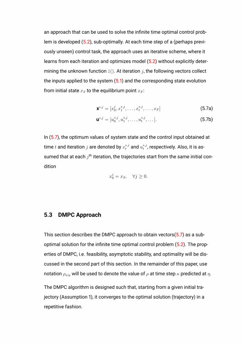
an approach that can be used to solve the infinite time optimal control prob-
lem is developed (5.2), sub-optimally. At each time step of a (perhaps previ-
ously unseen) control task, the approach uses an iterative scheme, where it
learns from each iteration and optimizes model (5.2) without explicitly deter-
mining the unknown function z(). At iteration j, the following vectors collect
the inputs applied to the system (5.1) and the corresponding state evolution
from initial state xS to the equilibrium point xF :
x∗,j = [xj0, x∗,j1 , . . . , x∗,jt , . . . , xF ] (5.7a)
u∗,j = [u∗,j0 , u∗,j1 , . . . , u∗,jt , . . . ]. (5.7b)
In (5.7), the optimum values of system state and the control input obtained at
time t and iteration j are denoted by x∗,jt and u∗,jt , respectively. Also, it is as-
sumed that at each jth iteration, the trajectories start from the same initial con-
dition
xj0 = xS, ∀j ≥ 0.
5.3 DMPC Approach
This section describes the DMPC approach to obtain vectors(5.7) as a sub-
optimal solution for the infinite time optimal control problem (5.2). The prop-
erties of DMPC, i.e. feasibility, asymptotic stability, and optimality will be dis-
cussed in the second part of this section. In the remainder of this paper, use
notation ρκ|η will be used to denote the value of ρ at time step κ predicted at η.
The DMPC algorithm is designed such that, starting from a given initial tra-
jectory (Assumption 1), it converges to the optimal solution (trajectory) in a
repetitive fashion.
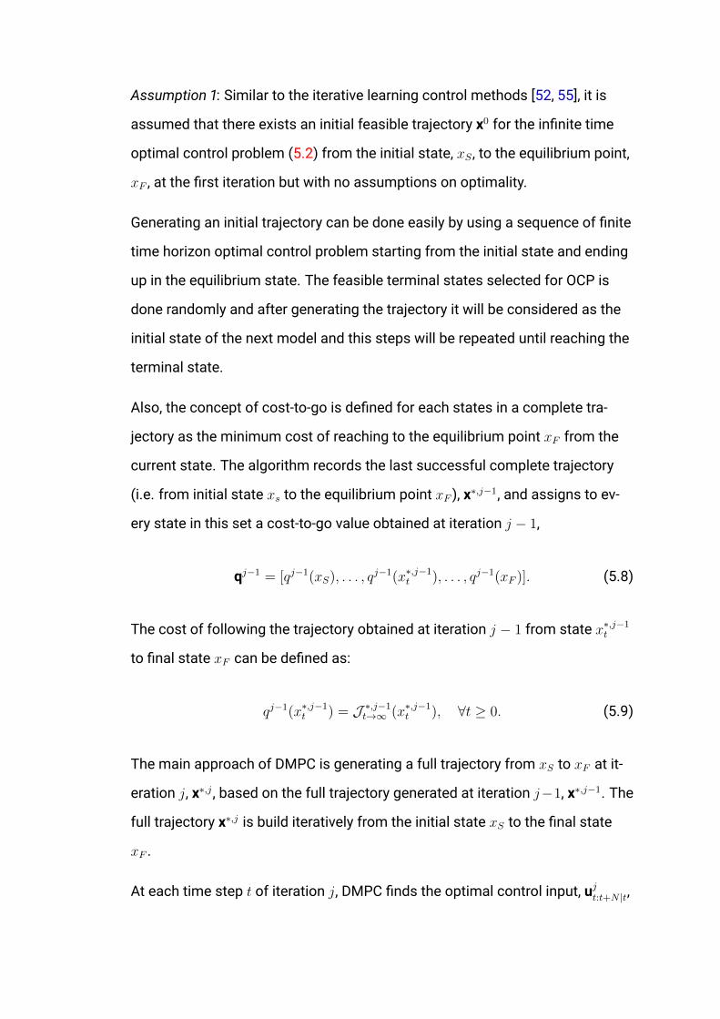
Assumption 1: Similar to the iterative learning control methods [52, 55], it is
assumed that there exists an initial feasible trajectory x0 for the infinite time
optimal control problem (5.2) from the initial state, xS , to the equilibrium point,
xF , at the first iteration but with no assumptions on optimality.
Generating an initial trajectory can be done easily by using a sequence of finite
time horizon optimal control problem starting from the initial state and ending
up in the equilibrium state. The feasible terminal states selected for OCP is
done randomly and after generating the trajectory it will be considered as the
initial state of the next model and this steps will be repeated until reaching the
terminal state.
Also, the concept of cost-to-go is defined for each states in a complete tra-
jectory as the minimum cost of reaching to the equilibrium point xF from the
current state. The algorithm records the last successful complete trajectory
(i.e. from initial state xs to the equilibrium point xF ), x∗,j−1, and assigns to ev-
ery state in this set a cost-to-go value obtained at iteration j − 1,
qj−1 = [qj−1(xS), . . . , qj−1(x∗,j−1t ), . . . , qj−1(xF )]. (5.8)
The cost of following the trajectory obtained at iteration j − 1 from state x∗,j−1t
to final state xF can be defined as:
qj−1(x∗,j−1t ) = J ∗,j−1
t→∞ (x∗,j−1t ), ∀t ≥ 0. (5.9)
The main approach of DMPC is generating a full trajectory from xS to xF at it-
eration j, x∗,j , based on the full trajectory generated at iteration j−1, x∗,j−1. The
full trajectory x∗,j is build iteratively from the initial state xS to the final state
xF .
At each time step t of iteration j, DMPC finds the optimal control input, ujt:t+N |t,

and associated trajectory, xjt:t+N |t
xjt:t+N |t = [x∗,jt , . . . , xjt+N |t] (5.10a)
ujt:t+N |t = [ujt|t, . . . , ujt+N−1|t]. (5.10b)
Where
x∗,jt = xjt|t (5.11)
is the current state of the system, which is considered as the optimal state
of the trajectory at iteration j at time t. DMPC selects the last state in (5.10a),
xjt+N |t, from a special set that results in a recursive feasibility guarantee. Be-
fore describing this set, two definitions are provided in the following: one-step
reachable set B and N -step reachable setRN(X0).
Definition 1 (one-step reachable set B): For the system (5.1), the one-step
reachable set from the set B is denoted as
Reach(B) =x ∈ Rn : ∃x(0) ∈ B,∃u(0) ∈ U , s.t. x = f(x(0), u(0))
(5.12)
Reach(B) is the set of states that can be reached from state x(0). N -step reach-
able set are defined by iterating Reach(.) computations [49].
Definition 2 (N-step reachable setRN(X0)): For a given initial set X0 ⊆ X , the
N -step reachable setRN(X0) of the system (5.1) subject to constraints (5.2d)
is defined as [49]:
Rt+1(X0) = Reach(Rt(X0)), R0(X0) = X0, t = 0, . . . , N − 1 (5.13)
At iteration j, DMPC is designed by repeatedly solving a finite time optimal
control problem in a receding horizon fashion to obtain state and control input
vectors (5.10). In the state vector (5.10a), the last state , xjt+N |t, is enforced to

be selected from set Sjt , that is defined as
Sjt =( ∞⋃t=0
x∗,j−1t
)∩RN(x∗,jt ). (5.14)
The first term in equation (5.14) is the set of all the states in the most recently
generated full trajectory (iteration j − 1), x∗,j−1, and the second term is N-step
reachable set from state x∗,jt .
All the states in trajectory x∗,j−1 are a member of control invariant set C ⊆ X ,
because, for every point in the set, there exists a feasible control action in in-
put vector u∗,j−1, that satisfies the state and control constraints and steers the
state of the system (5.1) toward the equilibrium point xF . Therefore, forcing
the controller to select the terminal state xjt+N |t from the set Sjt keeps the state
of the system in set C for time steps beyond the time horizon N [35], i.e.
if xjt+N ∈ C ⇒ xjt+N+k ∈ C ∀k > 0, (5.15)
On the other hand, trajectory xjt:t+N |t drives the system (5.1) from state x∗,jt to
one of the states in set Sjt in N time steps (see Figure (5.2)). Therefore, Sjt
is a subset of control invariant set and N-step reachable set, that make the
state x∗,jt to be a subset of maximal stabilizable set. Intuitively, this guaran-
tees the constraint satisfaction and feasibility for all time steps (t > 0) (the
feasibility will be proven in Theorem (3)). This means that the constraint satis-
faction at time steps beyond the time horizon does not depend on the length
of the time horizon, and N can be picked freely; in this work we will select
it to be small to speed up the algorithm. We denote each state in set Sjt by
si,jt ,∀i ∈ 1, . . . , |Sjt |.

Figure 5.2: The green area shows the N -step reachable set,RN(x∗,jt ), fromcurrent state, x∗,jt . Controllable set Sjt is illustrated by large blue dots and
dashed purple line segments are the optimal trajectories from current state toavailable states in controllable set Sjt .
5.3.1 Algorithmic Details
To find the (local) optimal trajectory xjt:t+N |t in (5.10), DMPC generates two tra-
jectories xjt:t+N |t and xjt:t+N |t−1, and selects the best of them based on their cost
as xjt:t+N |t. The second trajectory is build based on the previous trajectory and
is considered as a worst case, because it is readily available and if the first tra-
jectory is not better, the previously generated trajectory will be followed. We
explain how these trajectories are built in the following.
i) The first trajectory generated by DMPC is xjt:t+N |t, that is illustrated by a solid
black trajectory in Figure (5.3). This trajectory is the state vector associated
with the optimal control input ujt:t+N |t obtained from the following optimization
model over all the candidate terminal states that are reachable in N time steps
from the current state x∗,jt (equations 5.14). This set of terminal states is de-
picted by big blue points in Figure (5.2) and indexed by i ∈ 1, . . . , |Sjt | in the
following term
ujt:t+N |t = argminui,jt:t+N|t
J i,jt→t+N(x∗,jt ), ∀i ∈ 1, . . . , |Sjt |
, (5.16)
where J i,jt→t+N(x∗,jt ) is the predicted overall cost (i.e. summation of both the

Figure 5.3: DMPC generates two trajectories xjt:t+N |t (solid black) and xjt:t+N |t−1
(dashed green) at time step t of iteration j, and selects best of them
model-based∑h(.) and data-based
∑z(.) costs) enforced to the system be-
cause of following the control input ui,jt:t+N to reach the terminal state xi,jt+N |t =
si,jt . To simplify the mathematical notations, zi,jk|t will be used to show the pre-
dicted value of the unknown function following the control input ui,jt:t+N , instead
of z(xi,jk|t, ui,jk|t). Then the value of J i,j
t→t+N(x∗,jt ) can be defined as:
J i,jt→t+N(x∗,jt ) = J i,jt→t+N(x∗,jt ) +
t+N−1∑k=t
zi,jk|t. (5.17)
To find the optimal control input ujt:t+N |t in equation (5.16), we first use the fol-
lowing formulation to generate ui,jt:t+N |t and xi,jt:t+N |t from state x∗,jt toward termi-
nal state si,jt ∈ Sjt , ∀i ∈ 1, . . . , |S
jt |, and calculate the cost associated with the
model-based term, which is denoted by J i,jt→t+N(x∗,jt ) in equation (5.17)
J i,jt→t+N(x∗,jt ) = minui,jt:t+N
t+N−1∑k=t
`(xi,jk|t, ui,jk|t) + (N + 1)qj−1(xi,jt+N |t) (5.18a)
s.t. xi,jk+1|t = f(xi,jk|t, ui,jk|t) ∀k (5.18b)
xi,jt|t = x∗,jt (5.18c)
xi,jt+N |t = si,jt (5.18d)
xi,jk|t ∈ X , ui,jk|t ∈ U , ∀k. (5.18e)
In this model, the predictive controller generates the best trajectory to reach
state si,jt (i.e. enforced by constraint (5.18d)) and adds the cost to go (N +

1)qj−1(xi,jt+N |t) to compensate for the remaining cost from state si,jt to the final
state xF . We replace the stage cost h(., .) with positive definite function `(., .)
in the cost function as follows
`(xi,jk|t, ui,jk|t) = (xi,jk|t − x
i,jt+N |t)
TP (xi,jk|t − xi,jt+N |t) + (ui,jk|t)
TRui,jk|t, (5.19)
where P and R are positive (semi)definite tuning matrices. Function h() in the
general optimal control problem(5.2) penalizes the controller according to the
difference between the generated state xi,jk|t and the final state xF , but `(., .)
considers the selected terminal state xi,jt+N |t instead of xF . To compensate for
the remaining trajectory cost from xi,jt+N |t to xF , we add cost-to-go qj−1(xi,jt+N |t)
for each N + 1 states in the trajectory.
Constraint (5.18d) in optimization model (5.18) is enforced to the controller to
steer the system to a specific terminal state, si,jt .
The objective optimized by model (5.18) does not involve the cost value com-
ing from the data driven part,∑t+N−1
k=t zi,jk|t. However, given the trajectory xi,jt:t+N |t
generated by model (5.18), the value of this unknown function can be pre-
dicted by the external black-box system (depicted in Fig. 5.1) and added to
J i,jt→t+N(x∗,jt ) to find J i,jt→t+N(x∗,jt ) based on equation (5.17). Then, according to
(5.16), between all of the trajectories that start from x∗,jt and reach the termi-
nal states in set Sjt which are counted by index i (dashed purple trajectories
in Fig. 5.2), the trajectory that has the minimum cost value is selected and de-
noted xjt:t+N |t. That is, the result for (5.16) with the overall trajectory cost of
J jt→t+N(x∗,jt ).
ii) The second trajectory generated by DMPC is xjt:t+N |t−1, that is demonstrated
by a dashed green trajectory in Figure (5.3). In addition to xjt:t+N |t, another fea-
sible available trajectory starting from xS to xF can be obtained from the solu-
tion of the previous time step t − 1 at the current iteration j. This trajectory is

generated by applying one more step of the control input, ujt−1:t+N−1|t−1, to the
trajectory of the previous time step t − 1 and shifting its state one time step
toward the final state xF along the optimal trajectory of iteration j − 1. This
trajectory can be written as follows:
xjt:t+N |t−1 = [xjt|t−1, . . . , xjt+N−2|t−1, x
∗,j−1τ , x∗,j−1
τ+1 ] (5.20a)
ujt:t+N |t−1 = [ujt|t−1, . . . , ujt+N−2|t−1, u
∗,j−1τ ]. (5.20b)
x∗,j−1τ denotes the optimal terminal state selected from the last iteration (i.e.
the last generated complete trajectory) j − 1, and τ is the time index of this
state,
xjt+N−1|t−1 = x∗,j−1τ . (5.21)
The overall trajectory cost of xjt:t+N |t−1 is given by J jt→t+N |t−1(x∗,jt ) and is
J jt→t+N |t−1(x∗,jt ) =
t+N−2∑k=t
[`(xjk|t−1, u
jk|t−1) + zjk|t−1
]+Nqj−1(xjt+N−1|t−1) + qj−1(x∗,j−1
τ+1 ). (5.22)
J jt→t+N |t−1(x∗,jt ) is assumed to be an upper bound for J j
t→t+N(x∗,jt ), and in the
case that the controller cannot find a better trajectory, this trajectory will be
followed. This upper bound guarantees that the cost of trajectory in different
iterations do not worsen.
Therefore, the best trajectory of time step t and iteration j (ujt:t+N |t and xjt:t+N |t)
is selected between two obtained trajectories, xjt:t+N |t and xjt:t+N |t−1 based on
their cost values.
J jt→t+N(x∗,jt ) = minJ j
t→t+N(x∗,jt ),J jt→t+N |t−1(x∗,jt ). (5.23)
In other words, the algorithm selects between two trajectories: (a) the minimum-

cost feasible trajectory from t → t + N at time step t of iteration j, and (b) the
time-shifted trajectory from t − 1 → t + N that leverages information from the
prior time step t− 1 of iteration j.
After finding xjt:t+N |t and ujt:t+N |t, the first step of its control input is applied to
the system to push its state toward the equilibrium point,
u∗,jt = ujt|t, x∗,jt+1 = xjt+1|t. (5.24)
5.3.2 Theoretical Analysis
In the remainder of this section theoretical analyses of the algorithm are pro-
vided for the feasibility and optimality of the generated solutions.
Theorem 3. In the DMPC scheme with given system (5.1), cost function (5.16),
and constraints (5.18b) - (5.18e), if there is a feasible trajectory at iteration j − 1,
DMPC is feasible at the next iteration, j, as well.
Proof. To prove this theorem, first, we need to show that, given a feasible solu-
tion at time step t − 1 of iteration j, DMPC is feasible for the next time step, t,
too.
The solution of DMPC at iteration j − 1 is:
x∗,j−1 = [xS, x∗,j−11 , . . . , x∗,j−1
t , . . . , xF ], (5.25)
and at iteration j and time step t− 1 is:
xjt−1:t+N−1|t−1 = [x∗,jt−1, xjt|t−1, . . . , x
jt+N−1|t−1] (5.26a)
ujt−1:t+N−1|t−1 = [ujt−1|t−1, ujt|t−1, . . . , u
jt+N−2|t−1]. (5.26b)
According to constraint (5.18d), DMPC selects terminal state xjt+N−1|t−1 from

set Sjt−1 which is denoted by si,jt−1. Because si,jt−1 ∈ x∗,j−1, we can conclude that
xjt+N−1|t−1 ∈ x∗,j−1. Let us assume that xjt+N−1|t−1 = x∗,j−1τ . Based on the as-
sumption given in the theorem (existence of a feasible trajectory at iteration
j − 1), for every state in trajectory x∗,j−1 there is a feasible sequence of control
actions that satisfies the constraints and steers the system toward the final
state xF . This feasible trajectory for state x∗,j−1τ can be shown as:
x∗,j−1τ :∞ = [x∗,j−1
τ , x∗,j−1τ+1 , . . . , xF ] (5.27a)
u∗,j−1τ :∞ = [u∗,j−1
τ , u∗,j−1τ+1 , . . . ]. (5.27b)
Then there is at least one feasible trajectory at time step t and iteration j that
is constructed as:
xjt:∞ = [xjt|t−1, . . . , xjt+N−2|t−1, x
∗,j−1τ , x∗,j−1
τ+1 , . . . , xF ] (5.28a)
ujt:∞ = [ujt|t−1, . . . , ujt+N−2|t−1, u
∗,j−1τ , u∗,j−1
τ+1 , . . . ]. (5.28b)
This completes the proof of the statement that DMPC is feasible at time step t
if it is feasible at t − 1. Also, based on Assumption (1) and by induction we can
conclude that DMPC is feasible for all iterations and time steps.
It was shown that, given a feasible initial trajectory x0, the algorithm will be
feasible at every time steps of different iterations. Theorem (4) proves that,
the algorithm will finally converge to the equilibrium point xF , and Theorem (5)
proves that the performance index is non-increasing at every DMPC iteration.
The next two theorems follow almost the same approach provided in [52].
Theorem 4. In the DMPC scheme with given system (5.1), cost function (5.16),
constraints (5.18b) - (5.18e), and an initial feasible trajectory x0 , the equilibrium
point xF is asymptotically stable at every iteration j > 1.

Proof. Let us start with writing the overall optimal trajectory cost of state x∗,jt−1
J jt−1→t+N−1(x∗,jt−1) =
(N + 1)qj−1(xjt+N−1|t−1) +t+N−2∑k=t−1
[`(xjk|t−1, u
jk|t−1) + zjk|t−1
]= `(xjt−1|t−1, u
jt−1|t−1) + zjt−1|t−1 + qj−1(xjt+N−1|t−1)
+t+N−2∑k=t
`(xjk|t−1, ujk|t−1) +Nqj−1(xjt+N−1|t−1) + qj−1(x∗,j−1
τ+1 ), (5.29)
where
qj−1(x∗,j−1τ+1 ) =
∞∑k=τ+1
[h(x∗,j−1k , u∗,j−1
k
)+ z∗,j−1
k
]. (5.30)
Using equation (5.22),
J jt−1→t+N−1(x∗,jt−1) = J j
t→t+N |t−1(x∗,jt )
+ `(xjt−1|t−1, ujt−1|t−1) + zjt−1|t−1 + qj−1(xjt+N−1|t−1). (5.31)
Also, according to equation (5.23)
J jt→t+N(x∗,jt ) 6 J j
t→t+N |t−1(x∗,jt ). (5.32)
From equations (5.31) and (5.32) we conclude that
J jt→t+N(x∗,jt )− J j
t−1→t+N−1(x∗,jt−1) 6
− `(xjt−1|t−1, ujt−1|t−1)− zjt−1|t−1 − q
j−1(xjt+N−1|t−1) < 0,
∀t > 1, and ∀j > 1. (5.33)
This completes the proof of asymptotically stability of the equilibrium point
xF .
The next theorem guarantees that the generated trajectory is better than or
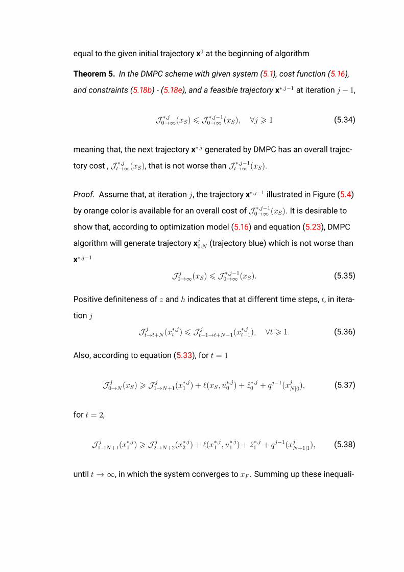
equal to the given initial trajectory x0 at the beginning of algorithm
Theorem 5. In the DMPC scheme with given system (5.1), cost function (5.16),
and constraints (5.18b) - (5.18e), and a feasible trajectory x∗,j−1 at iteration j − 1,
J ∗,j0→∞(xS) 6 J ∗,j−10→∞ (xS), ∀j > 1 (5.34)
meaning that, the next trajectory x∗,j generated by DMPC has an overall trajec-
tory cost , J ∗,jt→∞(xS), that is not worse than J ∗,j−1t→∞ (xS).
Proof. Assume that, at iteration j, the trajectory x∗,j−1 illustrated in Figure (5.4)
by orange color is available for an overall cost of J ∗,j−10→∞ (xS). It is desirable to
show that, according to optimization model (5.16) and equation (5.23), DMPC
algorithm will generate trajectory xj0:N (trajectory blue) which is not worse than
x∗,j−1
J j0→∞(xS) 6 J ∗,j−1
0→∞ (xS). (5.35)
Positive definiteness of z and h indicates that at different time steps, t, in itera-
tion j
J jt→t+N(x∗,jt ) 6 J j
t−1→t+N−1(x∗,jt−1), ∀t > 1. (5.36)
Also, according to equation (5.33), for t = 1
J j0→N(xS) > J j
1→N+1(x∗,j1 ) + `(xS, u∗,j0 ) + z∗,j0 + qj−1(xjN |0), (5.37)
for t = 2,
J j1→N+1(x∗,j1 ) > J j
2→N+2(x∗,j2 ) + `(x∗,j1 , u∗,j1 ) + z∗,j1 + qj−1(xjN+1|1), (5.38)
until t → ∞, in which the system converges to xF . Summing up these inequali-

Figure 5.4: Trajectory costs in different time steps. Orange: x∗,j−1. Blue: xj0:N .Green: xj1:N+1.
ties results in
J j0→N(xS) >
∞∑k=0
[`(x∗,jk , u∗,jk ) + z∗,jk + qj−1(xjk+N |k)
]. (5.39)
Where the right hand side of this inequality shows the sum of all stage costs
of optimal trajectory generated at iteration j
J ∗,j0→∞(xS) =∞∑k=0
[`(x∗,jk , u∗,jk ) + z∗,jk + qj−1(xjk+N |k)
], (5.40)
which yields the following inequality
J j0→N(xS) > J ∗,j0→∞(xS). (5.41)
From (5.35) and (5.41) we can easily conclude that
J ∗,j−10→∞ (xS) > J j
0→N(xS) > J ∗,j0→∞(xS), (5.42)
that shows, the overall cost of trajectories does not increase by the number of
iterations
J ∗,j0→∞(xS) 6 J ∗,j−10→∞ (xS), ∀j > 1, (5.43)
and the proof is complete.

5.4 Implementation Steps
According to equation (5.14), the DMPC algorithm needs the controllable set
Sjt at time step t and iteration j to select the best predicted terminal state.
However, calculating such a set is a time consuming process and because
it has to be executed for every state in different time steps t of iteration j, it
would affect the overall running time significantly. In this section we propose a
technique to avoid this volume of unnecessary calculations. It is assumed that
assumption (1) holds and there is a feasible trajectory from initial state xS to
the equilibrium point xF which is given as x0 and u0.
The main idea of this approach is, the algorithm will be given all of the states
of the trajectory generated at the previous iteration, x∗,j−1, as terminal candi-
date states
Sjt =∞⋃t=0
x∗,j−1t .
The algorithm selects the best predicted terminal state in this set from its cur-
rent state x∗,jt using the following integer programming optimization model:
J jt→t+N(x∗,jt ) = minujt:t+N
t+N−1∑k=t
`(xjk|t, ujk|t) + (N + 1)
|Qjt |∑
r=1
ξrqj−1(x∗,j−1
r ) (5.44a)
s.t. xjk+1|t = f(xjk|t, ujk|t) ∀k (5.44b)
xjt|t = x∗,jt (5.44c)
xjt+N |t =
|Qjt |∑
r=1
ξrx∗,j−1r (5.44d)
|Qjt |∑
r=1
ξr = 1 (5.44e)
ξr ∈ 0, 1, ∀r = 1, . . . , |Qjt | (5.44f)
xjk|t ∈ X , ujk|t ∈ U , ∀k, (5.44g)

where `(xjk|t, ujk|t) is defined in (5.19) and, in the second term of the cost func-
tion, qj−1 ∈ Qjt . Q
jt is the cost to go vector of terminal states in the set Sjt ,
which will be updated based on the current state x∗,jt . However, in the begin-
ning, the algorithm starts with Qjt =
⋃∞r=0 q
j−1(x∗,j−1r ). We define a binary deci-
sion variable ξr associated with each terminal state in the previous trajectory
x∗,j−1. ξr takes value one if the controller selects rth state from x∗,j−1 as the
desirable terminal state and assigns value zero to other states; see constraint
(5.44d). Also, using constraint (5.44e) we enforce the model to select only one
state. The output of this model is given by xjt:t+N |t and ujt:t+N |t.
Assume that the best terminal state selected by this model is x∗,j−1ι . Because
the model has not considered∑t+N−1
k=t zjk|t, the algorithm calls the available
exogenous data-driven system (e.g. a deep neural network) to calculate this
value for the generated trajectory xjt:t+N |t. Therefore, using equation (5.17),
J jt→t+N(x∗,jt ) can be found easily. After finding the overall trajectory cost from
current state x∗,jt that passes through terminal state x∗,j−1ι , the algorithm up-
dates the cost-to-go of state x∗,j−1ι in set Qj
t from qj−1(x∗,j−1ι ) to qj−1(x∗,j−1
ι ) +∑t+N−1k=t zjk|t. The algorithm keeps recording the index number of updated ter-
minal states of set Qjt in I. To clarify the reason for such an update, assume
that the algorithm launches model (5.44) again to find the best terminal state,
but by using the updated cost to go set Qjt . There are two possibilities about
the generated solution
1. The algorithm selects, again, the terminal state that has an updated cost
to go. In this case, this is the best terminal state between all the available
states that are reachable in N time steps and the algorithm stops. We
denote this best terminal state by, ι∗. This implies that
J jt→t+N(x∗,jt |r = ι∗) 6 J jt→t+N(x∗,jt |r /∈ I), ∀r = 1, . . . , |Qj
t |, (5.45)

then
J jt→t+N(x∗,jt |r = ι∗) 6 J j
t→t+N(x∗,jt |r ∈ I), ∀r = 1, . . . , |Qjt |. (5.46)
Inequality (5.45) means that, even though the algorithm has not tried the
rest of states in terminal states set Qjt , r /∈ I , the obtained cost of the
trajectory J jt→t+N(x∗,jt |r = ι∗) that passes from terminal state ι∗ has less
value than the terminal states that are not in I and they should be ne-
glected, because∑t+N−1
k=t zjk|t > 0 and adding it to J jt→t+N(x∗,jt ) to obtain
J jt→t+N(x∗,jt ) will worsen the cost ∀r /∈ I. And inequality (5.46) shows
that, the terminal state x∗,j−1ι∗ is better than all of the terminal states that
have updated cost to go, r ∈ I.
2. The algorithm selects the terminal state that is not in set I , ι /∈ I (i.e. its
cost-to-go value has not been updated). In this case the algorithm has
not found the best terminal state and the process should be repeated
again.
Using this approach, the algorithm will check the set of terminal states that
are potentially the optimal terminal state and ignore the other states in the
N -step reachable set of x∗,jt . After finding xjt:t+N |t, ujt:t+N |t and its optimal tra-
jectory cost J jt→t+N(x∗,jt ), the algorithm will generate the trajectory (ii) which is
a time shift trick on trajectory xjt−1:t+N−1|t−1 described by equation (5.20) as an
upper bound for cost value. Finally, according to equation (5.23) the optimal
trajectory xjt:t+N |t and ujt:t+N |t are obtained and the first step on control input is
applied.
Algorithm (2) presents this procedure in pseudocode.
In the last step (step 28), the similarity of the two last trajectories is consid-
ered as the termination criterion, in which different criteria can be set, e.g. run-
ning time, number of iterations, and etc. Also, it should be noted that Qjt and

Algorithm 2 : DMPC1: Set j = 0; convergence← 02: while (!convergence) do3: Update j ← j + 1 and set t = 04: Set x∗,10 ← xS , x0, u0, q0
5: while (x∗,jt 6= xF ) do6: Qj ←
⋃∞r=0 q
j−1(x∗,j−1r )
7: Set I ← ∅ and Qjt ← Qj
8: Set ι← −1, flag ← 19: while (flag) do
10: Solve IP model (5.44)11: Save the solution as X = [x∗,jt , . . . , x∗,j−1
ι ],12: ι is the index of the selected terminal state, (x∗,j−1
ι ) from set Qjt
13: Save the cost value as J jt→t+N(x∗,jt )14: if (ι /∈ I) then15: I ← ι ∪ I16: Feed X into the Exogenous System to receive the prediction17: [zjt|t, . . . , z
jt+N−1|t]
18: Qjt(x∗,j−1ι )← Qj
t(x∗,j−1ι ) +
∑t+N−1k=t zjk|t
19: else20: J j
t→t+N(x∗,jt )← J jt→t+N(x∗,jt )21: flag ← 022: end if23: end while24: Construct xjt:t+N |t−1 based on equation (5.20)25: Calculate J j
t→t+N |t−1(x∗,jt ) according to (5.22)26: Select the best of X and xjt:t+N |t−1 as x∗,jt:t+N |t based on J j
t→t+N(x∗,jt )
27: and J jt→t+N |t−1(x∗,jt )
28: Apply the first control input from u∗,jt:t+N |t29: Update t← t+ 130: end while31: if
∑∞t=0 |x
∗,jt − x
∗,j−1t | < ε then
32: convergence← 133: end if34: end while35: x∗,j = [xS, x
∗,j1 , . . . , x∗,jt , . . . , xF ] is optimal

Qj are two different sets. Qj is the overall cost to go vector that is calculated
after completing the trajectory x∗,j−1 and is counted by index r. This set stays
constant for the next iteration. But Qjt shows a special cost to go for state x∗,jt
that starts with Qj and is updated regularly as the exogenous (data-driven)
information is fed into the results of the integer program (step 16-18). The al-
gorithm counts the updated costs in this set by ι and x∗,j−1ι is the best terminal
state that has been selected by algorithm for state x∗,jt (step 11-12).
To calculate the complexity of the algorithm at iteration j, assume that at
each iteration of Branch and Bound relaxation, the algorithm solves a con-
vex quadratic model. Using the Interior Point Method (IPM), the computa-
tional complexity to find ε−scale optimum for a quadratic model is polyno-
mial in the size of the optimization model (n′) and required accuracy (ε), i.e.
O(n′log1/ε) [71]. The relaxation is implemented over the binary decision vari-
ables ξr ∀r defined for each terminal states in set Qjt . If the number of these
candidate states is T , the worst-case number of iterations of B&B algorithm is
exponential O(2T ). On the other hand, the size of model with time horizon N is
(n + m)N at each time step t. In the worst case, all of the candidate states are
tried to find the optimal candidate terminal state, which results in a computa-
tional complexity of O(2T (n + m)NTlog1/ε). The exponential part is dominant
and yields in O(2T ).
5.5 Example
In this section, proposed DMPC algorithm is applied on the constrained linear
and nonlinear models, that are motion planning of an autonomous vehicle with
linear and nonlinear dynamical systems.

5.5.1 Linear Dynamical System
In this section, the proposed DMPC algorithm is applied on the following con-
strained linear quadratic model, where z(vt) is an unknown function and it is
assumed that given a trajectory, there is a black-box system that can find the
corresponding vector vt and pass it to the controller. An example application
of such a setting (see Fig. 5.5) involves motion planning in an environment
with regions that have different cost values, where the state of these regions
are uncertain but the associated cost of selected states can be predicted by
a machine learning-based black box. In motion planning, such black-box vari-
ables could include predictions of other agents’ states or simply a dangerous
zone for a robot" . The infinite time optimal control problem is defined as:
J0→∞(x0) = minu
∞∑t=0
[h(xt, ut) + z(xt, ut, dt)] (5.47a)
s.t. xt+1 = Axt +But ∀t > 0 (5.47b)
x0 = [0 5 0 0]T (5.47c)
xt, yt ∈ R ∀t > 0 (5.47d)−4
−4
6
xtyt
6
4
4
∀t > 0 (5.47e)
−3
−3
6 ut 6
2
2
∀t > 0, (5.47f)
where xt = [xt yt xt yt]T , ut = [xt yt]
T and
A =
1 0 dt 0
0 1 0 dt
0 0 1 0
0 0 0 1
and B =
dt2
20
0 dt2
2
dt 0
0 dt
. (5.48)
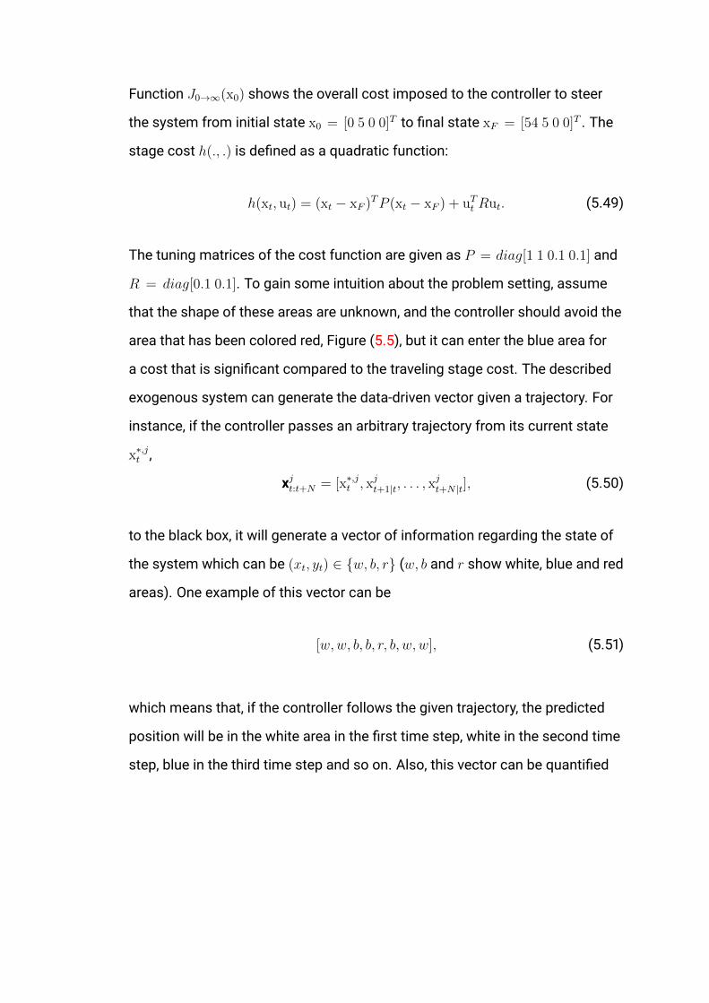
Function J0→∞(x0) shows the overall cost imposed to the controller to steer
the system from initial state x0 = [0 5 0 0]T to final state xF = [54 5 0 0]T . The
stage cost h(., .) is defined as a quadratic function:
h(xt, ut) = (xt − xF )TP (xt − xF ) + uTt Rut. (5.49)
The tuning matrices of the cost function are given as P = diag[1 1 0.1 0.1] and
R = diag[0.1 0.1]. To gain some intuition about the problem setting, assume
that the shape of these areas are unknown, and the controller should avoid the
area that has been colored red, Figure (5.5), but it can enter the blue area for
a cost that is significant compared to the traveling stage cost. The described
exogenous system can generate the data-driven vector given a trajectory. For
instance, if the controller passes an arbitrary trajectory from its current state
x∗,jt ,
xjt:t+N = [x∗,jt , xjt+1|t, . . . , xjt+N |t], (5.50)
to the black box, it will generate a vector of information regarding the state of
the system which can be (xt, yt) ∈ w, b, r (w, b and r show white, blue and red
areas). One example of this vector can be
[w,w, b, b, r, b, w, w], (5.51)
which means that, if the controller follows the given trajectory, the predicted
position will be in the white area in the first time step, white in the second time
step, blue in the third time step and so on. Also, this vector can be quantified

Figure 5.5: The cost of entering to the blue and red area are small and verybig, respectively. The down-left graph shows the cost-to-go vector for the
states of each separate trajectory, that from top (iteration 0 or initial trajectory)to down (last iteration) the convergence of trajectories can be seen. TheDown-right graph illustrates the overall trajectory cost of each trajectory.

based on the following piece-wise function
zt =
∞ if (xt, yt) ∈ obsred
k if (xt, yt) ∈ obsblue
0 o.w.
(5.52)
where k ∈ R+, which will result in a quantified version of vector (5.51)
[0, 0, k, k,∞, k, 0, 0]. (5.53)
In this scenario k = 5. Again, note that the controller knows nothing about
these regions a priori; it only explicitly knows about its own dynamics and per-
haps things like static obstacles that are a priori encoded in the problem for-
mulation. The controller feeds trajectory vector (5.50) to the exogenous data-
driven system and receives the predicted vector (5.53) without knowing how
(5.51) and (5.52) are calculated.
In this example the DMPC controller is expected to find the optimal trajectory
by using the outputs of the aforementioned black-box given a trajectory.
The DMPC (5.44) is constructed for each time step t from x0 to xF to generate
a full trajectory x∗,j . The algorithm will stop if∑∞
t=0 |xjt − xj−1
t | < 10−4. Also,
the time step and time horizon is assumed to be 0.5 second and N = 8, re-
spectively for this problem. Given the linear constraints, the cost function was
linearized by switching the tracking error to its 1-norm and adding associated
linear constraints to the model to have an overall MILP (Mixed Integer Linear
Programming) model. CPLEX and MATLAB were used to solve this problem.
The algorithm converges after 10 iterations.
The generated trajectories x∗,j ∀j > 0, cost to go for each states in different
trajectories qj ∀j, and overall trajectory cost of iterations qj(xj0) ∀j can be seen

Figure 5.6: Control input ut = [xt yt]T and states xt and yt in the steady state.
in graphs of Figure (5.5).
As the second example in this section, zt is defined to be an arbitrary non-
convex function that is again unknown for the controller. The black-box will
receive the information of predicted states of the system and calculates zt for
each of states and passes that to the controller. For instance, assume
zt = 30(e−x2t+y2t100 + e−(0.3xt+2)2−(0.3yt+2)2 + e−yt/70). (5.54)
Even in the case that this cost function is known to the controller, this Non-
linear Model Predictive Control (NMPC) can be changed to iterative DMPC
defined in model (5.44a) which can be optimized by MILP algorithms. In this
model, the algorithm treats z() as an unknown function and extracts special
samples (associated with the generated trajectory) from it and finally con-
verges to the (local) optimal trajectory as illustrated in Figure (5.7).
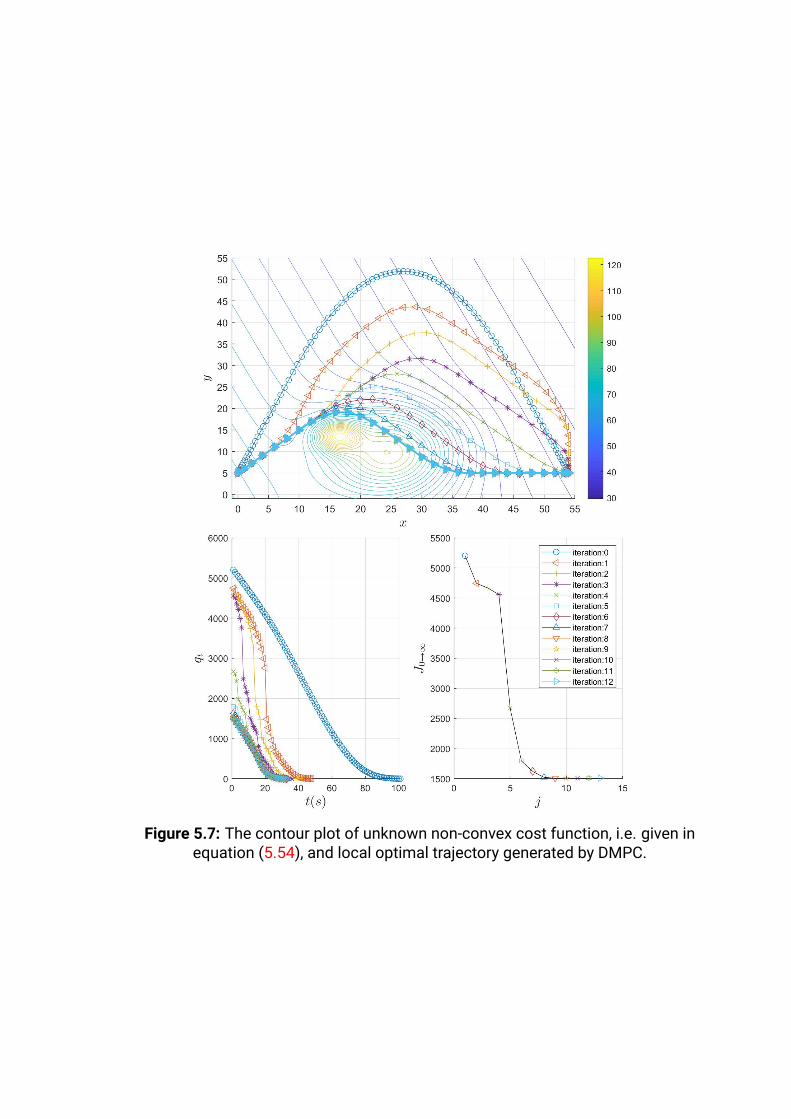
Figure 5.7: The contour plot of unknown non-convex cost function, i.e. given inequation (5.54), and local optimal trajectory generated by DMPC.

Figure 5.8: Control input ut = [xt yt]T and states xt and yt in the steady state
for the cost function of equation (5.54).
5.5.2 Nonlinear System
In this section a kinematic bicycle model in an inertial frame is used to de-
scribe the dynamics of the vehicle [72] (see Figure (5.9)). Also, z is an unknown
function and it is assumed that given a trajectory, there is a black-box system
that can find (predicts or measures) the corresponding vector and pass it to
the controller. The infinite time optimal control problem is defined as:
J0→∞(x0) = minu
∞∑t=0
[h(xt, ut) + z(xt, ut)] (5.55a)
s.t. xt = f(xt, ut) ∀t > 0 (5.55b)
xmin 6 xt 6 xmax ∀t > 0 (5.55c)
umin 6 ut 6 umax ∀t > 0, (5.55d)
x0 = xS (5.55e)

Figure 5.9: Kinematic Bicycle Model
where f(xt, ut) is defined as follows:
xt = vt cos(ψt + βt) (5.56a)
yt = vt sin(ψt + βt) (5.56b)
ψt =vtlrsin(βt) (5.56c)
vt = at (5.56d)
βt = tan−1(lr
lf + lrtan(δt)). (5.56e)
The state and control input vectors are xt = [xt yt ψt vt]T , ut = [δt at]
T , respec-
tively. xt and yt are the coordinates of the center of mass of the vehicle, ψt is
the heading angle, and vt is the velocity of the vehicle at time step t. lf and lr
show the distance of the center of the mass from the front and rear axles, re-
spectively. βt is the angle between the current velocity vector of the center of
mass and the longitudinal axis of the vehicle. The control input vector ut is
composed of the steering angle δt and the acceleration at that is defined for
the center of mass in the same direction as vt.
In constraint (5.55c), the upper and lower bounds of the state vector are as-
sumed to be xmin = [−∞ − ∞ 0 0]T and xmax = [+∞ + ∞ 2π 4]T . Also,
in constraint (5.55d), umin = [−π7− 1]T and umax = [π
71]T . Equality con-
straint (5.55e) represents the initial state x0, which in this case is assumed

to be xS = [0 5 π2
0].
Function J0→∞(x0) shows the overall cost imposed to the controller to steer
the system from initial state x0 to final state xF = [51 10 π10
1.1]T . The stage
cost h(., .) is defined as a quadratic function:
h(xt, ut) = (xt − xF )TP (xt − xF ) + uTt Rut. (5.57)
The tuning matrices of the cost function are given as P = diag[1 1 0.1 0.1] and
R = diag[0.01 0.01].
To gain some intuition about the problem setting, assume that an autonomous
ground robot is running on an uneven surface. The shape of this surface that
is an arbitrary non-convex function can be seen in figure (5.10) as a contour
plot. The height of points is presented by color bar, and the higher altitude lo-
cations has a more cost to travel.
The controller knows nothing about this function and it is only implemented
by the described exogenous system that functions as a black box to the con-
troller. In this example, the controller passes the generated trajectory from its
current state x∗,jt ,
xjt:t+N = [x∗,jt , xjt+1|t, . . . , xjt+N |t], (5.58)
to the black box, and the black box will produce a vector of cost values asso-
ciated with each state of the system. This data-driven vector is passed to the
controller to improve its prediction.
In this example, the DMPC controller is expected to improve the given initial
trajectory (blue circle trajectory in Figure (5.10)) in the presence of an unknown
cost function. The controller will use the most recently trajectory to converge
to an optimal trajectory at each iterations. We construct DMPC (5.44) for each
time step t from x0 to xF to generate a full trajectory x∗,j . The algorithm will

stop if∑∞
t=0 |xjt−xj−1
t | < 10−4. Also, the time step and time horizon is assumed
to be 0.5 second and N = 12, respectively for this problem. We used ACADO
Code Generation tool [73] with MATLAB to solve this problem, and DMPC con-
verged after 4 iterations.
The generated trajectories x∗,j ∀j > 0, cost to go for each states in different
trajectories qj ∀j, and overall trajectory cost of iterations qj(xj0) ∀j can be seen
in graphs of Figure (5.10). Also, Figure (5.11) illustrates the optimal steering
angle and acceleration/deceleration as control inputs, velocity and heading
angle at different time steps.
The autonomous reinforcement learning (RL) approaches typically require
large number of interactions with the unknown system/function to learn con-
trollers, which is a practical limitation in real cases, such as robots, where
these number of interactions can be impractical and time consuming [57]. Be-
cause in these group of applications Gaussian Process based MPC outper-
forms the RL approaches, we compare the performance of the DMPC with the
GP methods [44,58].
A Gaussian Process setting is considered where deterministic control inputs
ut is desirable that minimize cost function of the following finite time opti-
mal control problems which will be solved in a receding horizon fashion until
reaching the terminal state:
minut
Jt→t+N(xt) +
t+N∑k=t
Exk|t [z(xk|t)]. (5.59)
Jt→t+N(xt) denotes the conventional stage cost and Exk|t [z(xk|t)] denotes the
expected data-driven cost at time step k calculated at time t. To implement
the GP the training input and target data are defined to be x = [x y]T and z re-
spectively. A GP as a probabilistic, non-parametric model can be fully specified
by a mean functionm(.) and a covariance function σ2(.).

Figure 5.10: The contour plot of unknown non-convex cost function, and localoptimal trajectory generated by DMPC. The down-left graph shows the
cost-to-go vector for the states of each separate trajectory, that from top(iteration 0 or initial trajectory) to down (last iteration) the convergence of
trajectories can be seen. The Down-right graph illustrates the overall trajectorycost of each trajectory.

Figure 5.11: Control input ut = [δt at]T and states ψt and vt in the steady state.
The training data and corresponding training targets are collected as X =
[x1, x2, . . . ]T and z = [z1, z2, . . . ]
T . Given the test input denoted by x∗, the poste-
rior predictive distribution of z∗ is Gaussian p(z∗|x∗, X, z) = N(z∗|m(z∗), σ
2(z∗))
where
m(z∗) = k(X, x∗)T (K + σ2ε I)−1z, (5.60)
σ2(z∗) = k(x∗, x∗)− k(X, x∗)T (K + σ2ε I)−1k(X, x∗). (5.61)
σ2ε is variance of noise, k(., .) is defined as squared exponential (Radial Basis
Function, RBF) and K is the Gram matrix with entries of Ki,j = k(xi, xj) [48].
From equation (5.60), the cost function (5.59) can be rewritten as
minut
Jt→t+N(xt) +t+N∑k=t
∫z(xk|t)N (xk|t|µµµk|t,ΣΣΣk|t)dxk|t. (5.62)
It is assumed that p(xk|t) = N (xk|t|µµµk|t,ΣΣΣk|t), where µµµk|t and ΣΣΣk|t are the mean
and covariance of xk|t. Based on the mean function given in equation (5.60)
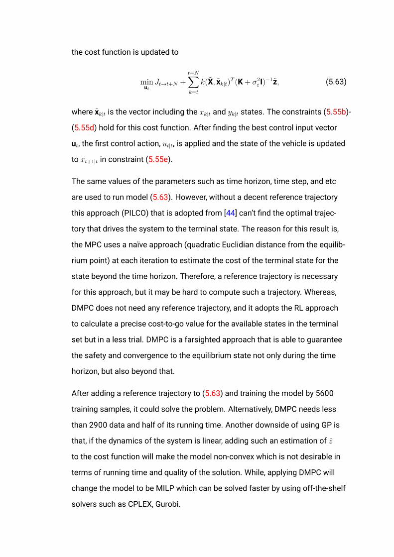
the cost function is updated to
minut
Jt→t+N +t+N∑k=t
k(X, xk|t)T (K + σ2ε I)−1z, (5.63)
where xk|t is the vector including the xk|t and yk|t states. The constraints (5.55b)-
(5.55d) hold for this cost function. After finding the best control input vector
ut, the first control action, ut|t, is applied and the state of the vehicle is updated
to xt+1|t in constraint (5.55e).
The same values of the parameters such as time horizon, time step, and etc
are used to run model (5.63). However, without a decent reference trajectory
this approach (PILCO) that is adopted from [44] can’t find the optimal trajec-
tory that drives the system to the terminal state. The reason for this result is,
the MPC uses a naïve approach (quadratic Euclidian distance from the equilib-
rium point) at each iteration to estimate the cost of the terminal state for the
state beyond the time horizon. Therefore, a reference trajectory is necessary
for this approach, but it may be hard to compute such a trajectory. Whereas,
DMPC does not need any reference trajectory, and it adopts the RL approach
to calculate a precise cost-to-go value for the available states in the terminal
set but in a less trial. DMPC is a farsighted approach that is able to guarantee
the safety and convergence to the equilibrium state not only during the time
horizon, but also beyond that.
After adding a reference trajectory to (5.63) and training the model by 5600
training samples, it could solve the problem. Alternatively, DMPC needs less
than 2900 data and half of its running time. Another downside of using GP is
that, if the dynamics of the system is linear, adding such an estimation of z
to the cost function will make the model non-convex which is not desirable in
terms of running time and quality of the solution. While, applying DMPC will
change the model to be MILP which can be solved faster by using off-the-shelf
solvers such as CPLEX, Gurobi.

5.6 Conclusions
In this chapter, a Data-and Model-driven Predictive Control (DMPC) algorithm
is presented to solve a model predictive control problem in which there is an
unknown function in the performance index or constraints that (a) is unknown
to the controller and (b) is interdependent with the decision variables (state
and control vector) of the MPC. The controller is designed to exploit an exist-
ing, exogenous data-driven system such as a black-box deep learning model,
along with model predictive control to find the optimal solution to this prob-
lem. To solve this problem, a controller is developed that conceptually borrows
from iterative learning controller but is intended for non-iterative or nonrepeti-
tive tasks. At each time step the controller optimizes via an iterative scheme,
which can use the generated results in the previous iteration and improve the
trajectory in the current iteration. The DMPC algorithm utilizes the last trajec-
tory only during its iteration scheme and builds an Integer Programming (IP)
model to solve this problem. The algorithm starts from an initial arbitrary tra-
jectory and it is proven that the algorithm will find a feasible trajectory in each
subsequent iteration, and the trajectory at each iteration is guaranteed to be
no worse than the previous one.
DMPC works with very little data and converges only in a few iterations. Two
examples with different forms of unknown functions and both linear and non-
linear dynamical systems were provided to examine the performance of the al-
gorithm. The first example of linear dynamic case is similar to obstacle avoid-
ance except that the controller can enter the area but for a cost, and more im-
portantly, the shape and the position of the obstacles are not known to the
controller. In the second example, the unknown stage cost is a nonlinear and
non-convex function and in both of examples it is assumed that there is an
exogenous system that provides the controller with samples from these func-

tions and the controller uses them to gradually converge to the optimal solu-
tion. In the nonlinear dynamical system the results were demonstrated for an
autonomous vehicle with a bicycle dynamics and its performance was com-
pared to Gaussian Processes.
Chapter 6
Summary of Contributions & Future
Work
After the emergence of autonomous vehicles, CAVs were developed to ad-
dress the safety and efficiency related concerns. CAVs allow keeping the inter-
vehicular distances as small as possible while guaranteeing safety which
brings up advantages such as more highway capacity usage, less aerody-
namic drag, minimum control effort, smoother driving, and less fuel consump-
tion. These benefits are due to sharing the motion policy of vehicles through a
wireless channel inside of a platoon. However, the V2V communication chan-
nel can be affected easily which in turn threatens the desired safety and effi-
ciency. PDR might fluctuate drastically even by changing the situation slightly.
Majority of the work in the literature assume a perfect communication channel
and wireless channel with time-varying delay which both approaches ignore
the relationships between the the states of two vehicles and surrounding envi-
ronment. In this dissertation two novel methodologies have been developed to
relax this assumption.
This chapter summarizes the presented contributions and provides some di-
rections for further studies in this field.

6.1 Summary of Contributions
In this dissertation two approaches GP-MPC (Gaussian Process-based Model
Predictive Controller) and DMPC (Data-and Model-Driven Predictive Control)
were presented to address an infinite time horizon optimal control problem in
which a part of model (cost function or constraints) is predicted or calculated
based on a data-driven system that is unknown to the controller. The appli-
cation for this problem can be sought in connected autonomous problem in
which all the autonomous vehicles are able to generate their optimal trajec-
tory for a number of time steps in the future and share it through a wireless
channel with the other members of the platoon. In this setting, the wireless
channel is assumed to be imperfect, meaning that the packet delivery rate is
not always perfect and varies from time to time as a function of the states of
two communicating vehicles and also the surrounding environment. But, this
function cannot be cast as an explicit mathematical formulation and it is as-
sumed that, given the states of two vehicles, this value can be predicted using
an exogenous system.
6.1.1 Gaussian Process-based Model Predictive Controller
GP-MPC as a data-driven Model Predictive Controller that leverages a Gaus-
sian Process to generate optimal motion policies was presented in chapter (3)
for connected autonomous vehicles in regions with uncertainty in the wire-
less channel. The communication channel between the vehicles of a platoon
is assumed to be influenced by numerous factors, e.g. the surrounding envi-
ronment, and the relative states of the connected vehicles, etc. In addition, the
trajectories of the vehicles depend significantly on the motion policies of the
preceding vehicle shared via the wireless channel and any delay can impact
the safety and optimality of its performance. In the presented algorithm, Gaus-
sian Process learns the wireless channel model and is involved in the Model
Predictive Controller to generate a control sequence that not only minimizes
the conventional motion costs, but also minimizes the estimated delay of the
wireless channel in the future. This results in a farsighted controller that maxi-
mizes the amount of transferred information beyond the controller’s time hori-
zon, which in turn helps to guarantee the safety and optimality of the gener-
ated trajectories in the future. To decrease computational cost, the algorithm
finds the reachable set from the current state and focuses on that region to
minimize the size of the kernel matrix and related calculations. In addition, an
efficient recursive approach was presented to decrease the time complexity of
developing the data-driven model and involving it in Model Predictive Control.
The capability of the presented algorithm was demonstrated in a simulated
scenario.
6.1.2 Learning Model Predictive Control
Chapter (4) presented a learning model predictive control approach to address
the problem of involving a data-driven variable in model predictive control. The
presented algorithm is iterative technique that utilizes its recently generated
trajectories to improve the current one. The algorithm builds a group of soft
constraints in the MPC and updates it regularly while exploring and converging
to the optimal trajectory.
This algorithm has the following advantages over GP-MPC:
• Despite GP-MPC, this algorithm does not transform the problem optimal
controlling a linear dynamical system to a nonlinear one.
• It does not need a reference trajectory, and an initial trajectory suffices.
• It does not require lots of data to generate its optimal trajectories.

• GP-MPC, similar to MPC, is unable to observe the state space beyond
the time horizon. This causes a local optimal trajectory in MPC (and in
some cases infeasible trajectory), but this algorithm does not have this
problem and will drive the system to the terminal state.
The learning model predictive controller approach is presented and tailored to
Connected Autonomous Vehicles (CAVs) applications. This algorithm is devel-
oped for the wireless channel with a limited number of discretized PDR values.
The proposed controller builds on previous work on nonlinear LMPC, adapting
its architecture and extending its capability to account for data-driven decision
variables that derive from an unknown or unknowable function. The chapter
presents the control design approach, and shows how to recursively construct
an outer loop candidate trajectory and an inner iterative LMPC controller that
converges to an optimal strategy over both model-driven and data-driven vari-
ables.
Simulation results to involve the variations of wireless channel in the model
predictive control of an autonomous vehicle showed the effectiveness of the
proposed control logic. The algorithm could recognize the area with imperfect
communication channel and based on the cost coefficients of cost function,
the controller was taking effective strategy to avoid the area. But the idea of
involving a soft constraint in the optimal control to build the area representing
the behavior of the wireless channel is demanding and is limited to discretized
values of PDR. PDR is a continuous parameter and an effective algorithm is
required to relax this limitation.
6.1.3 Data-and Model-Driven Predictive Control
In chapter (5), a Data-and Model-driven Predictive Control (DMPC) algorithm
is presented to solve a model predictive control problem in which there is an

unknown function in the performance index or constraints that (a) is unknown
to the controller and (b) is interdependent with the decision variables (state
and control vector) of the MPC. The controller is designed to exploit an exist-
ing, exogenous data-driven system such as a black-box deep learning model,
along with model predictive control to find the optimal solution to this prob-
lem. To solve this problem, a controller is developed that conceptually borrows
from iterative learning controller but is intended for non-iterative or nonrepeti-
tive tasks. At each time step the controller optimizes via an iterative scheme,
which can use the generated results in the previous iteration and improve the
trajectory in the current iteration. The DMPC algorithm utilizes the last trajec-
tory only during its iteration scheme and builds an Integer Programming (IP)
model to solve this problem. The algorithm starts from an initial arbitrary tra-
jectory and it is proven that the algorithm will find a feasible trajectory in each
subsequent iteration, and the trajectory at each iteration is guaranteed to be
no worse than the previous one.
DMPC works with very little data and converges only in a few iterations. Two
examples with different forms of unknown functions and dynamical systems
were presented to examine the performance of the algorithm in constrained
models. The first example is similar to obstacle avoidance except that the
controller can enter the area but for a cost, and more importantly, the shape
and the position of the obstacles are not known to the controller. In the sec-
ond example, the unknown stage cost is a nonlinear and non-convex function
and in both of examples it is assumed that there is an exogenous system that
provides the controller with samples from these functions and the controller
uses them to gradually converge to the optimal solution. The second example
was implemented for bot linear and nonlinear dynamical systems.

6.2 User guide for developed algorithms
This section provides some guidelines to use the developed algorithms in this
dissertation. Most important factors that are determinants can be listed as
follows:
• Existence of a reference trajectory that guides the controller to drive the
system from the initial to the terminal state
• Having a linear or nonlinear system
• Dealing with a continuous or discrete data-driven variable
• Availability of data for the mathematically unknown factor
• Importance of asymptotic stability of the equilibrium point
GP-MPC can be chosen when the dynamics of the system is nonlinear and
the data is readily available to explore the data-driven variable space. But, the
computational cost of GP-MPC is more than other algorithms developed in
this dissertation as it needs more data to build its proxy model. On the other
hand, it is easy and fast to adopt this approach for different applications. In
the case that reaching to the equilibrium is critical, it is notable that GP-MPC
does not guarantee the asymptotic stability of equilibrium point.
The preliminary version of learning based model predictive control can be
used when there is no reference trajectory. This algorithm requires an initial
trajectory from the initial to terminal state which is not expensive to generate.
If the dynamics of the system is linear and the data-driven variable can be de-
scribed by a few number of discrete values, this algorithm can converge to an
optimal solution fast. This algorithm will change the finite time optimal control
problem to a mixed integer linear programming model.

In the case that the data-driven variable is continuous or there are more than
few discrete value for it we should used DMPC which is a more general ap-
proach.
6.3 Future work
This section explains the possible future directions of the methodologies pre-
sented in this dissertation for the addressed problem.
In this dissertation, we tried to develop and study the characteristics of the
developed algorithms on two connected autonomous vehicles. Although this
is the building block of a platoon of vehicles and can be generalized to multi-
ple number of vehicles, a discussion on string stability of a platoon with more
than two vehicles can be fruitful to study the highway usage and overall perfor-
mance.
6.3.1 Iterative GP-MPC
In the GP-MPC algorithm, it is assumed that the data-driven variable is defined
using a proxy model developed by GP and is merged with MPC to solve for
both the model and data driven systems. Even though, two approaches were
devloped to overcome the computational burden of the algorithm, it still needs
improvement to be used in the real-world cases. To further reduce the compu-
tational cost of the algorithm, the algorithm can perform few iterations start-
ing from the trajectory that ignores the data-driven variable and explore the
state spaces in the neighborhood of the predicted trajectory by finite time op-
timal control problem for the data-driven variable. In the second iteration of
the process, the algorithm will add a very small proxy to OCP that is build by
GP to represent the approximated cost related to the data-driven variable. The
number of data to build this model in the first iteration will be zero, for the sec-
ond iteration N samples, for the third iteration 2N , and so on. Because the first
N − 1 states of the initial trajectory are optimal, the algorithm will start from a
good trajectory to converge to the final optimal trajectory.
6.3.2 Generating the initial solution for DMPC
In this work a systematic approach was not provided to generate an initial tra-
jectory for DMPC. As it was mentioned earlier, DMPC requires an initial fea-
sible trajectory from the initial to the terminal state. This initial solution can
be generated using a sequence of optimal control problem in which the initial
state of the current OCP is set to be the terminal state of the most recent OCP.
However, it was not clarified how the terminal state of the current OCP should
be selected.
The initial solution plays an important role in the optimality of the final solu-
tion. If this solution is generated inappropriately, the algorithm can easily get
stuck in a local optima without making a significant improvement in it.
6.3.3 Escaping Local Optima in DMPC
DMPC can stuck in a local optimal trajectory, and the current version of DMPC
that was presented in this dissertation is unable to escape such a solution.
The following feature can be added to DMPC to be called in this situations.
Preliminary steps of this approach are presented here.
In addition to a vector z, the exogenous system is called to measure/predict∂zt∂x, ∀x ∈ x∗,j−1. The gradient of the overall cost function∇J j−1 is defined
as:

∇J j−1 =∂z
∂x∗,j−1+
∂J
∂x∗,j−1(6.1)
where,
x∗,j−1 = [xS, x∗,j−11 , . . . , x∗,j−1
t , . . . , xF ] (6.2a)
∇J j−1 = [∇J j−10 ,∇J j−1
1 , . . . ,∇J j−1t , . . . ,∇J j−1
F ] (6.2b)
and
∇J j−1t =
∂z
∂x∗,j−1t
+∂J
∂x∗,j−1t
, ∀t (6.3)
At the end, the following constraints can be added to DMPC to force the con-
troller to not generate the most recently created full trajectory.
xjt ≤ xj−1t − α∇J j−1
t if ∇J j−1t ≥ 0 (6.4a)
xjt > xj−1t − α∇J j−1
t if ∇J j−1t < 0 (6.4b)
where α is a positive number as a tuning parameter. This approach can be ap-
plied in different ways. It can be implemented when two most recent full tra-
jectories are the same and also it can iterated for multiple time with a small
value of α and then be added as constraints.
6.3.4 Optimal control of unknown systems using DMPC
GPMPC has been used to control a system with unknown dynamics before.
The presented algorithm is called PILCO and it has been used to generate a
proxy model and optimally control an inverted pendulum [14, 44]. Applying
DMPC for such a problem setting is very interesting. In this problem, DMPC
will need more data from the solution space and some improvements can be
helpful to increase its performance for example, providing more candidate ter-

minal states same as Learning Model Predictive Control by keeping the previ-
ously generated full trajectories.
In addition, the ideas about generating the initial trajectory and escaping local
optima can be merged to be used in this problem to speed up the algorithm
and improve the final result.

Appendices
6.3.5 Notations
This section provides a complete list and a brief description for notations used
in this dissertation.
Table 6.1: Main Notations
Notation Meaning
xt system state at time tut control input at time tn number of states in system dynamicsm number of control inputs in system dynamicsN time horizonf known nonlinear mapX feasible state vector spaceU feasible control vector spacexS initial statexF final stateh() known functionz() unknown functionJ0→∞ overall cost functionj iteration indexx∗,j optimal state vector of iteration ju∗,j optimal control vector of iteration jx∗,jt optimal state at time t and iteration ju∗,jt optimal control input at time t and iteration jqj−1() cost-to-go value for each state at iteration j − 1
qj−1 cost-to-go vector at iteration j − 1
xjt:t+N |t optimal state from t to t+N estimated at tujt:t+N |t optimal control from t to t+N estimated at tujt+N−1|t optimal control at step t+ k estimated at txjt+N |t optimal state at step t+ k estimated at txF final stateh() known function

Notation Meaning
z() unknown functionJ0→∞ overall cost functionj iteration indexx∗,j optimal state vector of iteration ju∗,j optimal control vector of iteration jx∗,jt optimum state at time t and iteration ju∗,jt optimum control at time t and iteration jqj−1() cost-to-go value for each state at iteration j − 1
qj−1 cost-to-go vector at iteration j − 1
ujt:t+N |t optimal control from t to t+N estimated at txjt:t+N |t optimal state from t to t+N estimated at tujt+N−1|t optimal control at step t+ k estimated at txjt+N |t optimal state at step t+ k estimated at tReach(B) one-step reachable set BRN(X0) N -step reachable set X0
Sjt N -step reachable states of iteration j at time tC control invariant setsi,jt ith state in set Sjtui,jt:t+N |t optimal policy to reach terminal state si,jtxi,jt:t+N |t optimal state vector from control input ui,jt:t+N |tujt:t+N |t optimal control vector to generate xjt:t+N |txjt:t+N |t optimal state vector to the best state in set SjtJ i,jt→t+N() predicted overall cost of following policy
zi,jk|t predicted value of the unknown function followingthe control input ui,jt:t+N
J i,jt→t+N() model-based trajectory cost from x∗,jt to si,jt`(., .) alternative positive definite cost functionP positive semi-definite weighting matrixR positive definite weighting matrixJ jt→t+N() minimum overall trajectory cost from x∗,jt to the
best terminal state in Sjtx∗,j−1τ the optimal terminal state selected at the previous
time step to reach from state x∗,jt−1
u∗,j−1τ control input to drive the system from state x∗,j−1
τ
to x∗,j−1τ+1 along x∗,j−1
ujt:t+N |t−1 control to drive the system from x∗,jt to x∗,j−1τ+1

Notation Meaning
xjt:t+N |t−1 trajectory obtained by applying ujt−1:t+N−1|t−1
J jt→t+N |t−1The overall trajectory cost from x∗,jt to x∗,j−1
τ+1
J jt→t+N() the minimum trajectory cost from state x∗,jt
u∗,jt applied first step of optimal control policyx∗,jt+1 reached state by applying control input u∗,jtQjt cost to go vector of terminal states based on the
current state x∗,jtr binary variable indexξr rth binary variableι index of selected terminal state by model (5.44)ι∗ index of best terminal statexmin lower bound for feasible state spacexmax upper bound for feasible state spaceumin lower bound for feasible control spaceumax upper bound for feasible control spacext x coordination of the vehicleyt y coordination of the vehicleψt heading angle of the vehiclevt velocity of the vehicleβt angle of the velocity vector in the vehicleδt steering angle the vehicleat acceleration/deceleration of the vehiclex training input dataz training target dataX matrix of training input dataz vector of training target datax∗ test input dataz∗ test target dataσ2ε variance of noisem() mean function of z∗σ2() variance function of z∗K Gram matrixk(., .) entries of Kµµµk|t mean of xk|tΣΣΣk|t covariance of xk|t

References
[1] F. Gao, S. E. Li, Y. Zheng, and D. Kum, “Robust control of heterogeneous
vehicular platoon with uncertain dynamics and communication delay,” IET
Intelligent Transport Systems, vol. 10, no. 7, pp. 503–513, 2016.
[2] A. D. Ames, X. Xu, J. W. Grizzle, and P. Tabuada, “Control barrier function
based quadratic programs for safety critical systems,” IEEE Transactions
on Automatic Control, vol. 62, no. 8, pp. 3861–3876, 2016.
[3] A. Taylor, A. Singletary, Y. Yue, and A. Ames, “Learning for safety-critical
control with control barrier functions,” in Learning for Dynamics and Con-
trol, pp. 708–717, PMLR, 2020.
[4] X. Xu, P. Tabuada, J. W. Grizzle, and A. D. Ames, “Robustness of control
barrier functions for safety critical control,” IFAC-PapersOnLine, vol. 48,
no. 27, pp. 54–61, 2015.
[5] P. Varaiya, “Smart cars on smart roads: problems of control,” IEEE Trans-
actions on automatic control, vol. 38, no. 2, pp. 195–207, 1993.
[6] H. Jafarzadeh and C. Fleming, “Learning model predictive control for con-
nected autonomous vehicles,” in 2019 IEEE 58th Conference on Decision
and Control (CDC), pp. 2336–2343, IEEE, 2019.
[7] R. Schmied, H. Waschl, R. Quirynen, M. Diehl, and L. del Re, “Nonlinear
mpc for emission efficient cooperative adaptive cruise control,” IFAC-
papersonline, vol. 48, no. 23, pp. 160–165, 2015.

[8] T. Stanger and L. del Re, “A model predictive cooperative adaptive cruise
control approach,” in 2013 American Control Conference, pp. 1374–1379,
IEEE, 2013.
[9] H. Jafarzadeh and C. Fleming, “Dmpc: A data-and model-driven approach
to predictive control,” Automatica, vol. 131, p. 109729, 2021.
[10] W. Viriyasitavat, M. Boban, H.-M. Tsai, and A. Vasilakos, “Vehicular com-
munications: Survey and challenges of channel and propagation models,”
IEEE Vehicular Technology Magazine, vol. 10, no. 2, pp. 55–66, 2015.
[11] X. Liu, A. Goldsmith, S. S. Mahal, and J. K. Hedrick, “Effects of commu-
nication delay on string stability in vehicle platoons,” in ITSC 2001. 2001
IEEE Intelligent Transportation Systems. Proceedings (Cat. No. 01TH8585),
pp. 625–630, IEEE, 2001.
[12] A. Petrillo, A. Salvi, S. Santini, and A. S. Valente, “Adaptive multi-agents
synchronization for collaborative driving of autonomous vehicles with
multiple communication delays,” Transportation research part C: emerg-
ing technologies, vol. 86, pp. 372–392, 2018.
[13] J. G. Schneider, “Exploiting model uncertainty estimates for safe dynamic
control learning,” in Advances in neural information processing systems,
pp. 1047–1053, 1997.
[14] J. Kocijan, Modelling and control of dynamic systems using Gaussian pro-
cess models. Springer, 2016.
[15] S. Kamthe and M. P. Deisenroth, “Data-efficient reinforcement
learning with probabilistic model predictive control,” arXiv preprint
arXiv:1706.06491, 2017.
[16] D. A. Bristow, M. Tharayil, and A. G. Alleyne, “A survey of iterative learning
control,” IEEE control systems magazine, vol. 26, no. 3, pp. 96–114, 2006.

[17] Y. Wang, F. Gao, and F. J. Doyle III, “Survey on iterative learning control,
repetitive control, and run-to-run control,” Journal of Process Control,
vol. 19, no. 10, pp. 1589–1600, 2009.
[18] Z. Wang, Y. Bian, S. E. Shladover, and G. Wu, “A survey on cooperative lon-
gitudinal motion control of multiple connected and automated vehicles,”
IEEE Intelligent Transportation Systems Magazine, 2019.
[19] L.-h. Luo, H. Liu, P. Li, and H. Wang, “Model predictive control for adap-
tive cruise control with multi-objectives: comfort, fuel-economy, safety
and car-following,” Journal of Zhejiang University SCIENCE A, vol. 11, no. 3,
pp. 191–201, 2010.
[20] D. Corona and B. De Schutter, “Adaptive cruise control for a smart car: A
comparison benchmark for mpc-pwa control methods,” IEEE Transactions
on Control Systems Technology, vol. 16, no. 2, pp. 365–372, 2008.
[21] A. Iihoshi, S. Kobayashi, and Y. Furukawa, “Vehicle platoon control sys-
tem,” Feb. 29 2000. US Patent 6,032,097.
[22] J. K. Hedrick, D. McMahon, V. Narendran, and D. Swaroop, “Longitudinal
vehicle controller design for ivhs systems,” in 1991 American Control Con-
ference, pp. 3107–3112, IEEE, 1991.
[23] S. Kato, S. Tsugawa, K. Tokuda, T. Matsui, and H. Fujii, “Vehicle control al-
gorithms for cooperative driving with automated vehicles and intervehicle
communications,” IEEE Transactions on intelligent transportation systems,
vol. 3, no. 3, pp. 155–161, 2002.
[24] F. E. Sancar, B. Fidan, J. P. Huissoon, and S. L. Waslander, “Mpc based
collaborative adaptive cruise control with rear end collision avoidance,” in
2014 IEEE Intelligent Vehicles Symposium Proceedings, pp. 516–521, IEEE,
2014.

[25] Z. Wang, G. Wu, and M. J. Barth, “A review on cooperative adaptive cruise
control (cacc) systems: Architectures, controls, and applications,” in 2018
21st International Conference on Intelligent Transportation Systems (ITSC),
pp. 2884–2891, IEEE, 2018.
[26] M. Bashiri, H. Jafarzadeh, and C. H. Fleming, “Paim: Platoon-based au-
tonomous intersection management,” in 2018 21st International Confer-
ence on Intelligent Transportation Systems (ITSC), pp. 374–380, IEEE,
2018.
[27] M. Bashiri and C. H. Fleming, “A platoon-based intersection management
system for autonomous vehicles,” in 2017 IEEE Intelligent Vehicles Sympo-
sium (IV), pp. 667–672, IEEE, 2017.
[28] A. Uno, T. Sakaguchi, and S. Tsugawa, “A merging control algorithm based
on inter-vehicle communication,” in Proceedings 199 IEEE/IEEJ/JSAI In-
ternational Conference on Intelligent Transportation Systems (Cat. No.
99TH8383), pp. 783–787, IEEE, 1999.
[29] T. S. Rappaport et al., Wireless communications: principles and practice,
vol. 2. prentice hall PTR New Jersey, 1996.
[30] D. He, T. Qiu, and R. Luo, “Fuel efficiency-oriented platooning control of
connected nonlinear vehicles: A distributed economic mpc approach,”
Asian Journal of Control, 2019.
[31] W. B. Dunbar and D. S. Caveney, “Distributed receding horizon control of
vehicle platoons: Stability and string stability,” IEEE Transactions on Auto-
matic Control, vol. 57, no. 3, pp. 620–633, 2011.
[32] Y. Zhou, M. Wang, and S. Ahn, “Distributed model predictive control ap-
proach for cooperative car-following with guaranteed local and string sta-
bility,” Transportation research part B: methodological, vol. 128, pp. 69–86,
2019.

[33] A. A. Malikopoulos and L. Zhao, “A closed-form analytical solution for op-
timal coordination of connected and automated vehicles,” in 2019 Ameri-
can Control Conference (ACC), pp. 3599–3604, IEEE, 2019.
[34] Y. Bian, Y. Zheng, W. Ren, S. E. Li, J. Wang, and K. Li, “Reducing time head-
way for platooning of connected vehicles via v2v communication,” Trans-
portation Research Part C: Emerging Technologies, vol. 102, pp. 87–105,
2019.
[35] R. Firoozi, S. Nazari, J. Guanetti, R. O’Gorman, and F. Borrelli, “Safe adap-
tive cruise control with road grade preview and v2v communication,” arXiv
preprint arXiv:1810.09000, 2018.
[36] L. Makarem and D. Gillet, “Model predictive coordination of autonomous
vehicles crossing intersections,” in 16th International IEEE Conference on
Intelligent Transportation Systems (ITSC 2013), pp. 1799–1804, IEEE, 2013.
[37] C. Liu, S. Lee, S. Varnhagen, and H. E. Tseng, “Path planning for au-
tonomous vehicles using model predictive control,” in 2017 IEEE Intelligent
Vehicles Symposium (IV), pp. 174–179, IEEE, 2017.
[38] D. A. Schoenwald, “Auvs: In space, air, water, and on the ground,” IEEE
Control Systems Magazine, vol. 20, no. 6, pp. 15–18, 2000.
[39] E. Fridman, “New lyapunov–krasovskii functionals for stability of linear re-
tarded and neutral type systems,” Systems & control letters, vol. 43, no. 4,
pp. 309–319, 2001.
[40] L. Wu, J. Yang, C. Han, L. Liu, and D. Sun, “Model predictive cruise control
of heterogeneous vehicle systems,” in 2019 Chinese Control And Decision
Conference (CCDC), pp. 6131–6136, IEEE, 2019.
[41] P. Yang, Y. Tang, M. Yan, and X. Zhu, “Consensus based control algorithm
for nonlinear vehicle platoons in the presence of time delay,” International
Journal of Control, Automation and Systems, vol. 17, no. 3, pp. 752–764,
2019.
[42] J. K. Hale and S. M. V. Lunel, Introduction to functional differential equa-
tions, vol. 99. Springer Science & Business Media, 2013.
[43] D. O. T. Hs, “Vehicle Safety Communications Project - Final Report,” Com-
munications, no. April, p. 44, 2006.
[44] M. Deisenroth and C. E. Rasmussen, “Pilco: A model-based and data-
efficient approach to policy search,” in Proceedings of the 28th Interna-
tional Conference on machine learning (ICML-11), pp. 465–472, 2011.
[45] M. Cutler and J. P. How, “Efficient reinforcement learning for robots using
informative simulated priors,” in 2015 IEEE International Conference on
Robotics and Automation (ICRA), pp. 2605–2612, IEEE, 2015.
[46] A. Yahya, A. Li, M. Kalakrishnan, Y. Chebotar, and S. Levine, “Collective
robot reinforcement learning with distributed asynchronous guided policy
search,” in 2017 IEEE/RSJ International Conference on Intelligent Robots
and Systems (IROS), pp. 79–86, IEEE, 2017.
[47] R. S. Sutton and A. G. Barto, Reinforcement learning: An introduction. MIT
press, 2018.
[48] C. E. Rasmussen, “Gaussian processes in machine learning,” in Summer
School on Machine Learning, pp. 63–71, Springer, 2003.
[49] F. Borrelli, A. Bemporad, and M. Morari, Predictive control for linear and
hybrid systems. Cambridge University Press, 2017.
[50] E. Juárez-Ruiz, R. Cortés-Maldonado, and F. Pérez-Rodríguez, “Relation-
ship between the inverses of a matrix and a submatrix,” Computación y
Sistemas, vol. 20, no. 2, pp. 251–262, 2016.

[51] F. Zhang, The Schur complement and its applications, vol. 4. Springer Sci-
ence & Business Media, 2006.
[52] U. Rosolia and F. Borrelli, “Learning model predictive control for iterative
tasks. a data-driven control framework,” IEEE Transactions on Automatic
Control, vol. 63, no. 7, pp. 1883–1896, 2018.
[53] M. Brunner, U. Rosolia, J. Gonzales, and F. Borrelli, “Repetitive learning
model predictive control: An autonomous racing example,” in 2017 IEEE
56th Annual Conference on Decision and Control (CDC), pp. 2545–2550,
IEEE, 2017.
[54] U. Rosolia, X. Zhang, and F. Borrelli, “Robust learning model predictive
control for iterative tasks: Learning from experience,” in 2017 IEEE 56th
Annual Conference on Decision and Control (CDC), pp. 1157–1162, IEEE,
2017.
[55] U. Rosolia and F. Borrelli, “Learning model predictive control for iterative
tasks. a data-driven control framework,” IEEE Transactions on Automatic
Control, vol. 63, no. 7, pp. 1883–1896, 2017.
[56] H. Jafarzadeh and C. H. Fleming, “An exact geometry–based algorithm
for path planning,” International Journal of Applied Mathematics and Com-
puter Science, vol. 28, no. 3, pp. 493–504, 2018.
[57] M. P. Deisenroth, D. Fox, and C. E. Rasmussen, “Gaussian processes for
data-efficient learning in robotics and control,” IEEE transactions on pat-
tern analysis and machine intelligence, vol. 37, no. 2, pp. 408–423, 2013.
[58] S. Kamthe and M. Deisenroth, “Data-efficient reinforcement learning with
probabilistic model predictive control,” in International Conference on Arti-
ficial Intelligence and Statistics, pp. 1701–1710, PMLR, 2018.

[59] M. Behl, F. Smarra, and R. Mangharam, “Dr-advisor: A data-driven demand
response recommender system,” Applied Energy, vol. 170, pp. 30–46,
2016.
[60] F. Smarra, G. D. Di Girolamo, V. De Iuliis, A. Jain, R. Mangharam, and
A. D’Innocenzo, “Data-driven switching modeling for mpc using regression
trees and random forests,” Nonlinear Analysis: Hybrid Systems, vol. 36,
p. 100882, 2020.
[61] T. M. Moerland, J. Broekens, and C. M. Jonker, “Model-based reinforce-
ment learning: A survey,” arXiv preprint arXiv:2006.16712, 2020.
[62] S. Curi, F. Berkenkamp, and A. Krause, “Efficient model-based reinforce-
ment learning through optimistic policy search and planning,” Advances in
Neural Information Processing Systems, vol. 33, 2020.
[63] J. H. Lee and K. S. Lee, “Iterative learning control applied to batch
processes: An overview,” Control Engineering Practice, vol. 15, no. 10,
pp. 1306–1318, 2007.
[64] K. S. Lee and J. H. Lee, “Convergence of constrained model-based predic-
tive control for batch processes,” IEEE Transactions on Automatic Control,
vol. 45, no. 10, pp. 1928–1932, 2000.
[65] S.-C. Hsu, C.-L. Huang, and C.-H. Chuang, “Vehicle detection using simpli-
fied fast r-cnn,” in 2018 International Workshop on Advanced Image Tech-
nology (IWAIT), pp. 1–3, IEEE, 2018.
[66] J. Cao, C. Song, S. Song, S. Peng, D. Wang, Y. Shao, and F. Xiao, “Front ve-
hicle detection algorithm for smart car based on improved ssd model,”
Sensors, vol. 20, no. 16, p. 4646, 2020.
[67] H. Manh and G. Alaghband, “Scene-lstm: A model for human trajectory
prediction,” arXiv preprint arXiv:1808.04018, 2018.

[68] W. Liu and Y. Shoji, “Deepvm: Rnn-based vehicle mobility prediction to
support intelligent vehicle applications,” IEEE Transactions on Industrial
Informatics, vol. 16, no. 6, pp. 3997–4006, 2019.
[69] H. Jafarzadeh and C. Fleming, “Learning model predictive control for con-
nected autonomous vehicles,” in 2019 IEEE 58th Conference on Decision
and Control (CDC), pp. 2336–2343, 2019.
[70] E. Soltanaghaei, M. Elnaggar, K. Kleeman, K. Whitehouse, and C. Fleming,
“Characterizing uncertainties of wireless channels in connected vehicles,”
in The 25th Annual International Conference on Mobile Computing and Net-
working, pp. 1–3, 2019.
[71] Y. Ye and E. Tse, “An extension of karmarkar’s projective algorithm for
convex quadratic programming,” Mathematical programming, vol. 44,
no. 1-3, pp. 157–179, 1989.
[72] J. Kong, M. Pfeiffer, G. Schildbach, and F. Borrelli, “Kinematic and dynamic
vehicle models for autonomous driving control design,” in 2015 IEEE Intel-
ligent Vehicles Symposium (IV), pp. 1094–1099, IEEE, 2015.
[73] B. Houska, H. Ferreau, and M. Diehl, “An Auto-Generated Real-Time Itera-
tion Algorithm for Nonlinear MPC in the Microsecond Range,” Automatica,
vol. 47, no. 10, pp. 2279–2285, 2011.