Model Predictive Control - Stanford University...Model Predictive Control • linear convex optimal control • ﬁnite horizon approximation • model predictive control • fast

Model Predictive Control

• linear convex optimal control

• finite horizon approximation

• model predictive control

• fast MPC implementations

• supply chain management

Prof. S. Boyd, EE364b, Stanford University

Linear time-invariant convex optimal control

minimize J =∑∞

t=0 ℓ(x(t), u(t))

subject to u(t) ∈ U , x(t) ∈ X , t = 0, 1, . . .

x(t + 1) = Ax(t) + Bu(t), t = 0, 1, . . .

x(0) = z.

• variables: state and input trajectories x(0), x(1), . . . ∈ Rn,u(0), u(1), . . . ∈ Rm

• problem data:

– dynamics and input matrices A ∈ Rn×n, B ∈ Rn×m

– convex stage cost function ℓ : Rn × Rm → R, ℓ(0, 0) = 0– convex state and input constraint sets X , U , with 0 ∈ X , 0 ∈ U– initial state z ∈ X

Prof. S. Boyd, EE364b, Stanford University 1

Greedy control

• use u(t) = argminw{ℓ(x(t), w) | w ∈ U , Ax(t) + Bw ∈ X}

• minimizes current stage cost only, ignoring effect of u(t) on future,except for x(t + 1) ∈ X

• typically works very poorly; can lead to J = ∞ (when optimal u givesfinite J)


‘Solution’ via dynamic programming

• (Bellman) value function V (z) is optimal value of control problem as afunction of initial state z

• can show V is convex

• V satisfies Bellman or dynamic programming equation

V (z) = inf {ℓ(z, w) + V (Az + Bw) | w ∈ U , Az + Bw ∈ X}

• optimal u given by

u⋆(t) = argminw∈U, Ax(t)+Bw∈X

(ℓ(x(t), w) + V (Ax(t) + Bw))


• intepretation: term V (Ax(t) + Bw) properly accounts for future costsdue to current action w

• optimal input has ‘state feedback form’ u⋆(t) = φ(x(t))


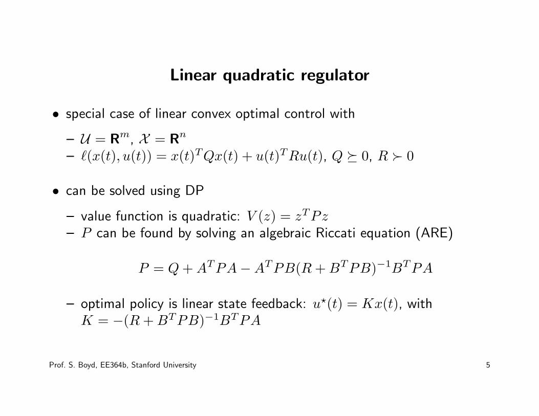
Linear quadratic regulator

• special case of linear convex optimal control with

– U = Rm, X = Rn

– ℓ(x(t), u(t)) = x(t)TQx(t) + u(t)TRu(t), Q � 0, R ≻ 0

• can be solved using DP

– value function is quadratic: V (z) = zTPz

– P can be found by solving an algebraic Riccati equation (ARE)

P = Q + ATPA − ATPB(R + BTPB)−1BTPA

– optimal policy is linear state feedback: u⋆(t) = Kx(t), withK = −(R + BTPB)−1BTPA


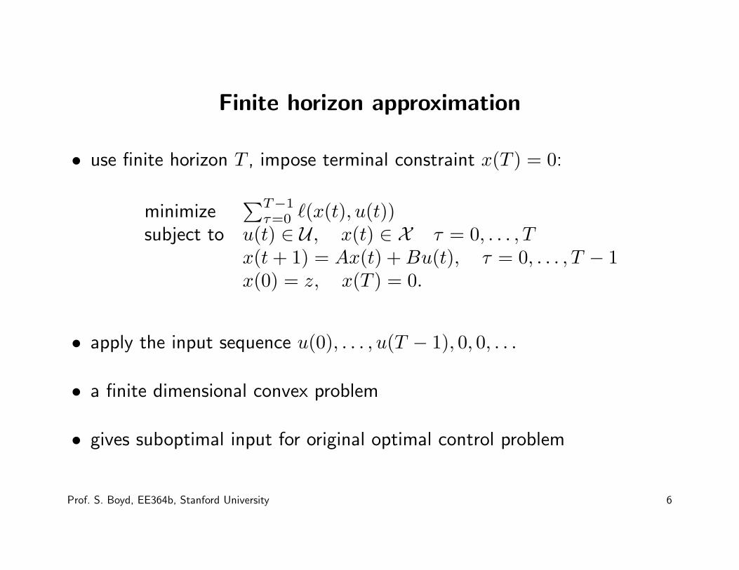
Finite horizon approximation

• use finite horizon T , impose terminal constraint x(T ) = 0:

minimize∑T−1

τ=0 ℓ(x(t), u(t))subject to u(t) ∈ U , x(t) ∈ X τ = 0, . . . , T

x(t + 1) = Ax(t) + Bu(t), τ = 0, . . . , T − 1x(0) = z, x(T ) = 0.

• apply the input sequence u(0), . . . , u(T − 1), 0, 0, . . .

• a finite dimensional convex problem

• gives suboptimal input for original optimal control problem


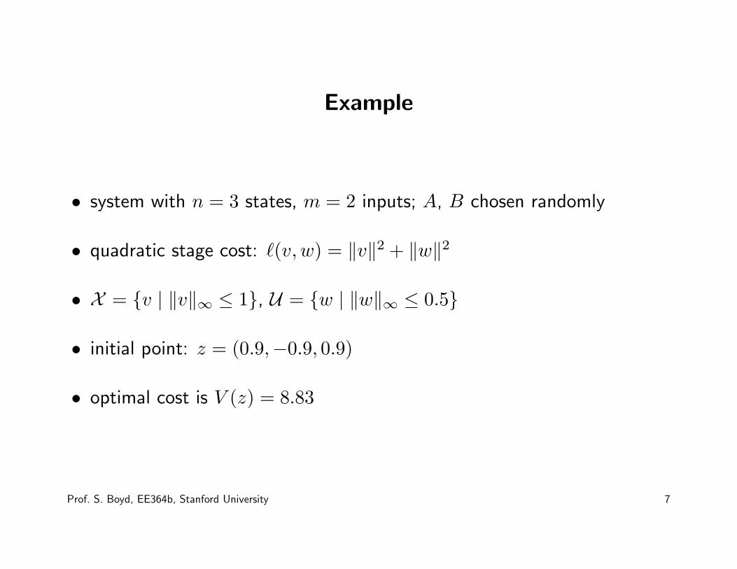
Example

• system with n = 3 states, m = 2 inputs; A, B chosen randomly

• quadratic stage cost: ℓ(v, w) = ‖v‖2 + ‖w‖2

• X = {v | ‖v‖∞ ≤ 1}, U = {w | ‖w‖∞ ≤ 0.5}

• initial point: z = (0.9,−0.9, 0.9)

• optimal cost is V (z) = 8.83


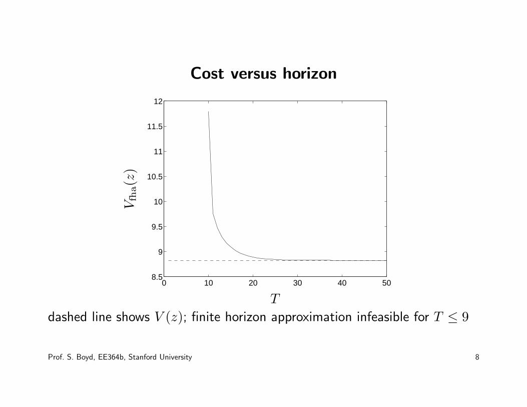
Cost versus horizon

0 10 20 30 40 508.5

9

9.5

10

10.5

11

11.5

12

Vfh

a(z

)

T

dashed line shows V (z); finite horizon approximation infeasible for T ≤ 9


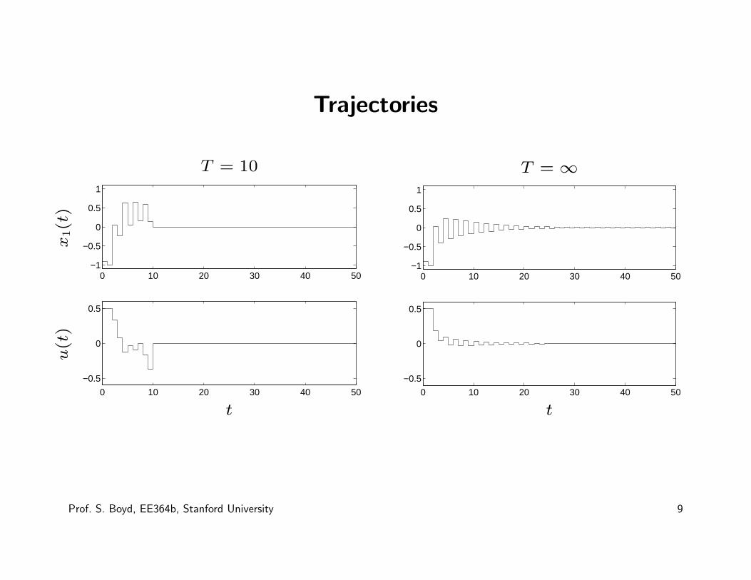
Trajectories

0 10 20 30 40 50−1

−0.5

0

0.5

1

0 10 20 30 40 50

−0.5

0

0.5

T = 10

x1(t

)u(t

)

t

0 10 20 30 40 50−1

−0.5

0

0.5

1

0 10 20 30 40 50

−0.5

0

0.5

T = ∞

t


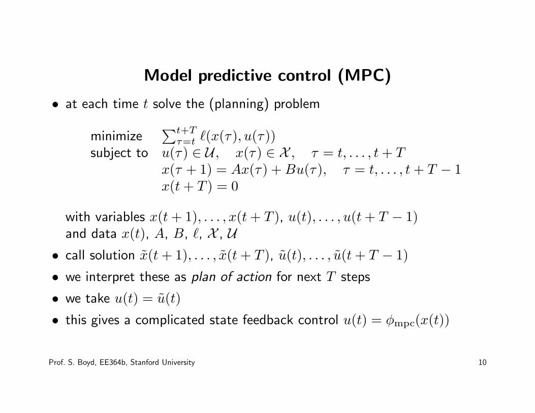
Model predictive control (MPC)

• at each time t solve the (planning) problem

minimize∑t+T

τ=t ℓ(x(τ), u(τ))subject to u(τ) ∈ U , x(τ) ∈ X , τ = t, . . . , t + T

x(τ + 1) = Ax(τ) + Bu(τ), τ = t, . . . , t + T − 1x(t + T ) = 0

with variables x(t + 1), . . . , x(t + T ), u(t), . . . , u(t + T − 1)and data x(t), A, B, ℓ, X , U

• call solution x(t + 1), . . . , x(t + T ), u(t), . . . , u(t + T − 1)

• we interpret these as plan of action for next T steps

• we take u(t) = u(t)

• this gives a complicated state feedback control u(t) = φmpc(x(t))


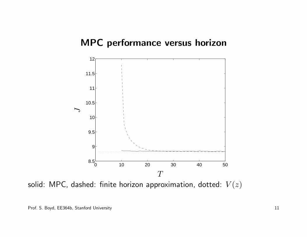
MPC performance versus horizon

0 10 20 30 40 508.5

9

9.5

10

10.5

11

11.5

12

J

T

solid: MPC, dashed: finite horizon approximation, dotted: V (z)


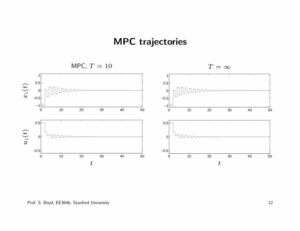
MPC trajectories

0 10 20 30 40 50−1

−0.5

0

0.5

1

0 10 20 30 40 50

−0.5

0

0.5

MPC, T = 10

x1(t

)u

1(t

)

t

0 10 20 30 40 50−1

−0.5

0

0.5

1

0 10 20 30 40 50

−0.5

0

0.5

T = ∞

t


MPC

• goes by many other names, e.g., dynamic matrix control, recedinghorizon control, dynamic linear programming, rolling horizon planning

• widely used in (some) industries, typically for systems with slowdynamics (chemical process plants, supply chain)

• MPC typically works very well in practice, even with short T

• under some conditions, can give performance guarantees for MPC


Variations on MPC

• add final state cost V (x(t + T )) instead of insisting on x(t + T ) = 0

– if V = V , MPC gives optimal input

• convert hard constraints to violation penalties

– avoids problem of planning problem infeasibility

• solve MPC problem every K steps, K > 1

– use current plan for K steps; then re-plan


Explicit MPC

• MPC with ℓ quadratic, X and U polyhedral

• can show φmpc is piecewise affine

φmpc(z) = Kjz + gj, z ∈ Rj

R1, . . . ,RN is polyhedral partition of X

(solution of any QP is PWA in righthand sides of constraints)

• φmpc (i.e., Kj, gj, Rj) can be computed explicitly, off-line

• on-line controller simply evaluates φmpc(x(t))(effort is dominated by determining which region x(t) lies in)


• can work well for (very) small n, m, and T

• number of regions N grows exponentially in n, m, T

– needs lots of storage– evaluating φmpc can be slow

• simplification methods can be used to reduce the number of regions,while still getting good control


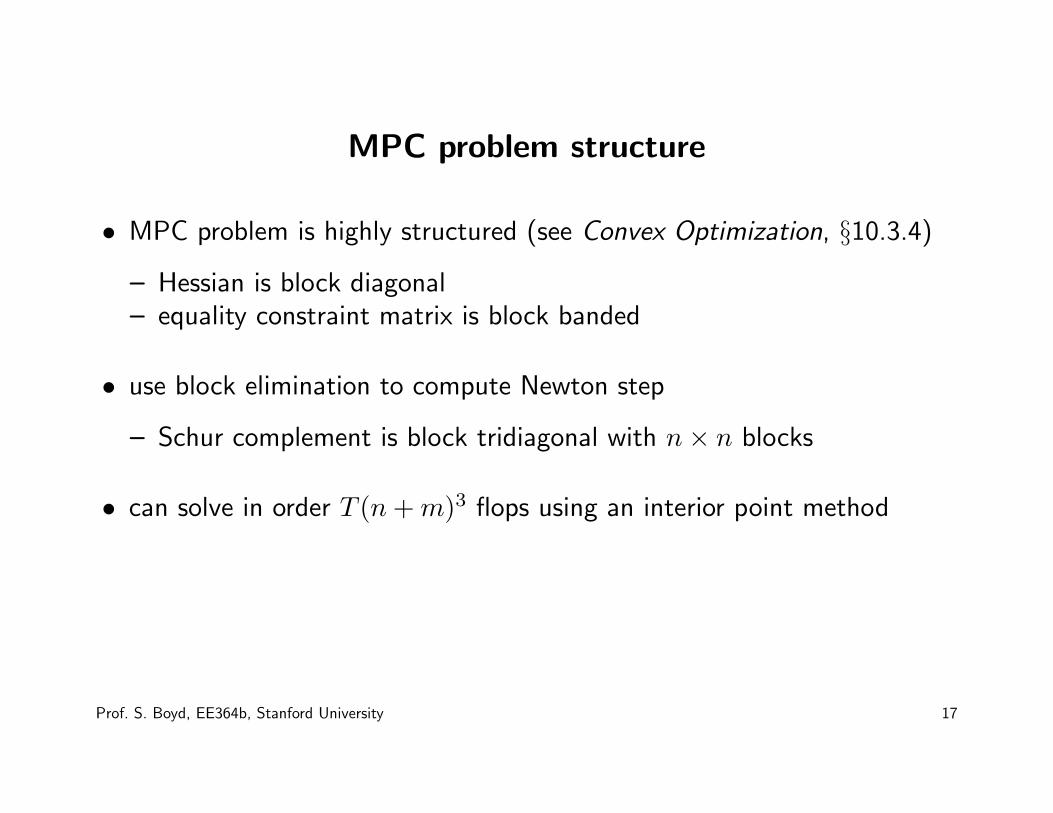
MPC problem structure

• MPC problem is highly structured (see Convex Optimization, §10.3.4)

– Hessian is block diagonal– equality constraint matrix is block banded

• use block elimination to compute Newton step

– Schur complement is block tridiagonal with n × n blocks

• can solve in order T (n + m)3 flops using an interior point method


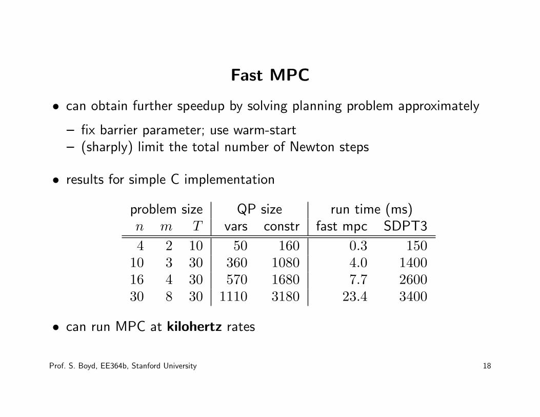
Fast MPC

• can obtain further speedup by solving planning problem approximately

– fix barrier parameter; use warm-start– (sharply) limit the total number of Newton steps

• results for simple C implementation

problem size QP size run time (ms)n m T vars constr fast mpc SDPT3

4 2 10 50 160 0.3 15010 3 30 360 1080 4.0 140016 4 30 570 1680 7.7 260030 8 30 1110 3180 23.4 3400

• can run MPC at kilohertz rates


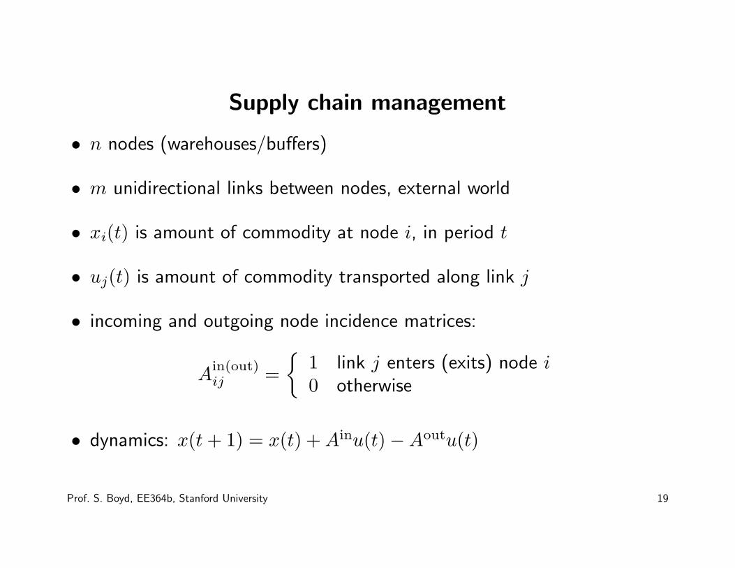
Supply chain management

• n nodes (warehouses/buffers)

• m unidirectional links between nodes, external world

• xi(t) is amount of commodity at node i, in period t

• uj(t) is amount of commodity transported along link j

• incoming and outgoing node incidence matrices:

Ain(out)ij =

{1 link j enters (exits) node i

0 otherwise

• dynamics: x(t + 1) = x(t) + Ainu(t) − Aoutu(t)


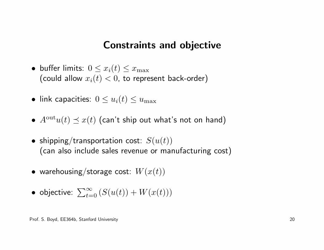
Constraints and objective

• buffer limits: 0 ≤ xi(t) ≤ xmax

(could allow xi(t) < 0, to represent back-order)

• link capacities: 0 ≤ ui(t) ≤ umax

• Aoutu(t) � x(t) (can’t ship out what’s not on hand)

• shipping/transportation cost: S(u(t))(can also include sales revenue or manufacturing cost)

• warehousing/storage cost: W (x(t))

• objective:∑∞

t=0 (S(u(t)) + W (x(t)))


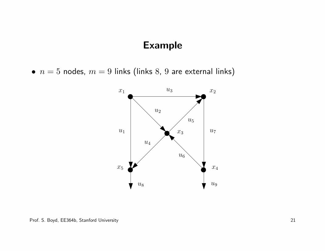
Example

• n = 5 nodes, m = 9 links (links 8, 9 are external links)

x1 x2

x3

x4x5

u1

u2

u3

u4

u5

u6

u7

u8 u9


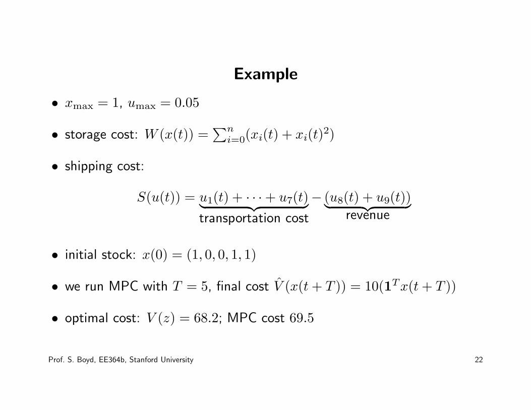
Example

• xmax = 1, umax = 0.05

• storage cost: W (x(t)) =∑n

i=0(xi(t) + xi(t)2)

• shipping cost:

S(u(t)) = u1(t) + · · · + u7(t)︸︷︷︸

transportation cost

− (u8(t) + u9(t))︸︷︷︸

revenue

• initial stock: x(0) = (1, 0, 0, 1, 1)

• we run MPC with T = 5, final cost V (x(t + T )) = 10(1Tx(t + T ))

• optimal cost: V (z) = 68.2; MPC cost 69.5


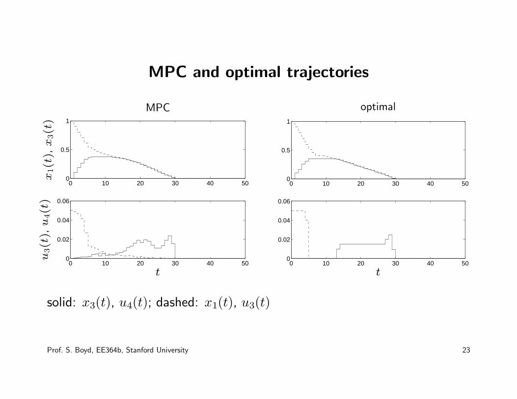
MPC and optimal trajectories

0 10 20 30 40 500

0.5

1

0 10 20 30 40 500

0.02

0.04

0.06

x1(t

),x

3(t

)u

3(t

),u

4(t

)

t

MPC

0 10 20 30 40 500

0.5

1

0 10 20 30 40 500

0.02

0.04

0.06

t

optimal

solid: x3(t), u4(t); dashed: x1(t), u3(t)


Variations on optimal control problem

• time varying costs, dynamics, constraints

– discounted cost– convergence to nonzero desired state– tracking time-varying desired trajectory

• coupled state and input constraints, e.g., (x(t), u(t)) ∈ P(as in supply chain management)

• slew rate constraints, e.g., ‖u(t + 1) − u(t)‖∞ ≤ ∆umax

• stochastic control: future costs, dynamics, disturbances not known(next lecture)


Documents

Model Predictive Control - Stanford University...Model Predictive Control • linear convex optimal control • ﬁnite horizon approximation • model predictive control • fast