u n i ve r s i t y o f co pe n h ag e n

Københavns Universitet

The influence of firn air transport processes and radiocarbon production on gasrecords from polar firn and iceBuizert, Christo

Publication date:2012

Document VersionEarly version, also known as pre-print

Citation for published version (APA):Buizert, C. (2012). The influence of firn air transport processes and radiocarbon production on gas records frompolar firn and ice. Center for Ice & Climate: Niels Bohr Institutet.

Download date: 12. Jul. 2018

F A C U L T Y O F S C I E N C E U N I V E R S I T Y O F C O P E N H A G E N

Ph.D. ThesisChristo Buizert

The influence of firn air transport processes and radio-carbon production on gas records from polar firn and ice

Academic supervisor:Prof. Thomas Blunier

Submitted 21/10/2011

Abstract

Air bubbles found in polar ice cores preserve a record of past atmospheric composi-tion up to 800 kyr back in time. The composition of the bubbles is not identical tothe ancient atmosphere, as it is influenced by processes prior to trapping, within theice sheet itself, and during sampling and storage. Understanding of these processesis essential for a correct interpretation of ice core gas records. In this work we focuson transport processes in the porous firn layer prior to bubble trapping, and in situcosmogenic radiocarbon (14C) production in ice.

First, we present a review of firn air studies. We describe the firn air samplingprocess, the relevant physical characteristics of firn, the different mechanisms of airtransport, and the effects of firn air transport on gas records.

Second, we present a characterization of the firn air transport properties of theNEEM deep drilling site in Northern Greenland (77.45◦N 51.06◦W). The depth-diffusivity relationship needs to be reconstructed using reference tracers of knownatmospheric history. We present a novel method of characterizing the firn transportusing ten tracers simultaneously, thus constraining the effective diffusivity betterthan the commonly used single-tracer method would. A comparison between tworeplicate boreholes drilled 64 m apart shows differences in measured mixing ratioprofiles that exceed the experimental error, which we attribute to lateral inhomo-geneities in firn stratigraphy. We find evidence that diffusivity does not vanishcompletely in the lock-in zone, as is commonly assumed. Six state-of-the-art firn airtransport models are tuned to the NEEM site; all models successfully reproduce thedata within a 1σ Gaussian distribution. We present the first intercomparison studyof firn air models, where we introduce diagnostic scenarios designed to probe specificaspects of the model physics. Our results show that there are major differences inthe way the models handle advective transport, and that diffusive fractionation ofisotopes in the firn is poorly constrained by the models.

Third, we describe an empirical method to calculate the magnitude of diffusivefractionation (DF) of isotopes in the ice core record. Our method 1) requires littlecomputational effort, 2) uses only commonly available ice core data, 3) does not re-

i

ii

quire knowledge of the (unknown) true atmospheric history, and 4) is arguably moreaccurate than a full modeling study. The method consists of an analytical expressionfor the DF in combination with a parameterization of gas age at the lock-in depthbased on five modern firn air sites. We test the accuracy and dynamic responseof our method by comparing it to a firn air transport model for two modern, well-characterized firn air sites. We find an excellent agreement on timescales relevantfor ice core data (≥ 100 years). We apply our method to CH4, CO2 and N2O mixingratios found in ice cores, and find that δ13C–CH4 is the only trace gas isotopic signalfor which the diffusive correction should always be applied during transitions. Weapply the DF correction to published δ13C–CH4 records over the last glacial termi-nation and the 8.2 kyr event. In both cases the DF correction exceeds the analyticalprecision of the data during abrupt transitions. We argue that the corrected timeseries are more consistent than the uncorrected ones. We show that our method hasan uncertainty of around 15% in the case thermal fractionation-corrected δ15N–N2

data is used, and around 20% when uncorrected δ15N–N2 data is used. We arguethat our empirical method is more accurate than the alternative of a full modelingstudy.

Fourth, we describe in detail the development of the CIC firn air model. Wederive expressions for the air velocity in the open porosity, the bubble trappingrate, and for the pressurization of closed bubbles due to firn compaction. We testthese equations for NEEM and South Pole, and find they predict the total air contentaccurately within 3%. We give a complete mathematical description of trace gas masstransfer in the open porosity, and its numerical implementation using the Crank-Nicolson method. We present a new way to reconstruct the effective diffusivity profilewith depth. We show how mixing ratios in the closed porosity can be calculated,and show how the trapping process broadens the age distribution. We find theadditional broadening due to trapping to be negligible at NEEM, because of its highaccumulation and relatively long lock-in zone. At South pole there is significantbroadening due to the lower accumulation rate and short lock-in zone.

Fifth, we combine cosmic ray scaling and production estimates with a 2-D iceflow line model to study cosmogenic 14C production at the Taylor Glacier blue icearea, Antarctica. We find that 1) 14C production by thermal neutron capture inair bubbles is negligible, 2) including ice flow patterns caused by basal topographycan lead to surface 14C activities that differ by up to 25% from activities calculatedusing an ablation-only approximation, which is used in all prior work, and 3) athigh ablation margin sites, solar variability modulates the strength of the dominantspallogenic production by 10%. We introduce two methods to parameterize verticalstrain rates in modeling ice flow, and assess which method is more reliable for TaylorGlacier. Finally, we present a sensitivity study from which we conclude that uncer-tainties in published cosmogenic production rates are the largest source of potentialerror. The results presented here can inform ongoing and future 14C and ice flowstudies at ice margin sites, including important paleoclimatic applications such asthe reconstruction of paleoatmospheric 14C content of methane.

Resume

Luftbobler fanget i polare iskerner giver en optegnelse af fortidens atmosfæriskesammensætning op til 800.000 ar tilbage i tiden. Sammensætningen af gassen iboblerne er ikke identisk med fortidens atmosfære, da den bliver pavirket af processerforud for formationen af boblerne, i isen, og senere ved prøvetagning og opbevaring.Forstaelse af disse processer er afgørende for fortolkning af iskernes gas optegnelser.I dette studie fokusere vi pa transport processerne i den porøse firn før formationenaf boblerne, og in situ kosmogonisk kulstof (14C) produktion i is.

Først præsenterer vi en gennemgang af firn luft undersøgelser. Vi beskriverprøvetagning af firn luf, de relevante fysiske egenskaber ved firn, de forskellige formerfor lufttransport, og virkningerne af firn lufttransport pa gas optegnelser i iskerner.

For det andet, præsentere vi en karakteristik af firn lufttransport egenskaber afNEEM dybe borested i det nordlige Grønland (77,45◦N 51,06◦W). Dybde-diffusivitetforhold skal rekonstrueres ved hjælp af sporstoffers kendte atmosfærisk historie. Vipræsenterer en ny metode til at karakterisere firn transport ved hjælp af ti sporstof-fer samtidigt, og dermed bestemme den effektive diffusivitet bedre end den almin-deligt anvendte sporing af et enkelt sporestof. En sammenligning mellem to rep-likere boringer, boret 64 m fra hinanden, viser forskelle i malt mixing-ratio profiler,forskellen overstiger den eksperimentelle fejl, dette tilskriver vi lateral uensarteth-eder i firn stratigrafi. Vi finder, at diffusivitet ikke forsvinde fuldstændig i lock-in zone, som normalt antages. Seks state-of-the-art firn lufttransport modeller ertunet til NEEM stedet; alle modeller gengive data inden for en 1σ Gauss distribu-tion. Vi præsenterer det første sammenligningsprogrammer for undersøgelse af firnluft-modeller, hvor vi indføre diagnostiske scenarier designet til at sonde specifikkeaspekter af den modelleret fysik. Vores resultater viser, at der er store forskelle iden made modelleren handterer advective transport, og den diffusive fraktioneringaf isotoper i firn er darligt bestem af modellerne.

For det tredje, beskriver vi en empirisk metode til at beregne størrelsen af diffu-sive fraktionering (DF) af isotoper i iskerne optegnelser. Vores metode 1) kræver lilleberegningsmæssige indsats, 2) bruger tilgængelige iskerne data, 3) kræver ikke kend-

iii

iv

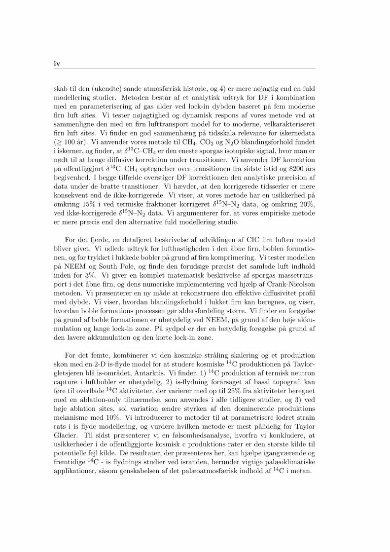
skab til den (ukendte) sande atmosfærisk historie, og 4) er mere nøjagtig end en fuldmodellering studier. Metoden bestar af et analytisk udtryk for DF i kombinationmed en parameterisering af gas alder ved lock-in dybden baseret pa fem modernefirn luft sites. Vi tester nøjagtighed og dynamisk respons af vores metode ved atsammenligne den med en firn lufttransport model for to moderne, velkarakteriseretfirn luft sites. Vi finder en god sammenhæng pa tidsskala relevante for iskernedata(≥ 100 ar). Vi anvender vores metode til CH4, CO2 og N2O blandingsforhold fundeti iskerner, og finder, at δ13C–CH4 er den eneste sporgas isotopiske signal, hvor man ernødt til at bruge diffusive korrektion under transitioner. Vi anvender DF korrektionpa offentliggjort δ13C–CH4 optegnelser over transitionen fra sidste istid og 8200 arsbegivenhed. I begge tilfælde overstiger DF korrektionen den analytiske præcision afdata under de bratte transitioner. Vi hævder, at den korrigerede tidsserier er merekonsekvent end de ikke-korrigerede. Vi viser, at vores metode har en usikkerhed paomkring 15% i ved termiske fraktioner korrigeret δ15N–N2 data, og omkring 20%,ved ikke-korrigerede δ15N–N2 data. Vi argumenterer for, at vores empiriske metodeer mere præcis end den alternative fuld modellering studie.

For det fjerde, en detaljeret beskrivelse af udviklingen af CIC firn luften modelbliver givet. Vi udlede udtryk for lufthastigheden i den abne firn, boblen formatio-nen, og for trykket i lukkede bobler pa grund af firn komprimering. Vi tester modellenpa NEEM og South Pole, og finde den forudsige præcist det samlede luft indholdinden for 3%. Vi giver en komplet matematisk beskrivelse af sporgas massetrans-port i det abne firn, og dens numeriske implementering ved hjælp af Crank-Nicolsonmetoden. Vi præsenterer en ny made at rekonstruere den effektive diffusivitet profilmed dybde. Vi viser, hvordan blandingsforhold i lukket firn kan beregnes, og viser,hvordan boble formations processen gør aldersfordeling større. Vi finder en forøgelsepa grund af boble formationen er ubetydelig ved NEEM, pa grund af den høje akku-mulation og lange lock-in zone. Pa sydpol er der en betydelig forøgelse pa grund afden lavere akkumulation og den korte lock-in zone.

For det femte, kombinerer vi den kosmiske straling skalering og et produktionskøn med en 2-D is-flyde model for at studere kosmiske 14C produktionen pa Taylor-gletsjeren bla is-omradet, Antarktis. Vi finder, 1) 14C produktion af termisk neutroncapture i luftbobler er ubetydelig, 2) is-flydning forarsaget af basal topografi kanføre til overflade 14C aktiviteter, der varierer med op til 25% fra aktiviteter beregnetmed en ablation-only tilnærmelse, som anvendes i alle tidligere studier, og 3) vedhøje ablation sites, sol variation ændre styrken af den dominerende produktionsmekanisme med 10%. Vi introducerer to metoder til at parametrisere lodret strainrats i is flyde modellering, og vurdere hvilken metode er mest palidelig for TaylorGlacier. Til sidst præsenterer vi en følsomhedsanalyse, hvorfra vi konkludere, atusikkerheder i de offentliggjorte kosmisk c produktions rater er den største kilde tilpotentielle fejl kilde. De resultater, der præsenteres her, kan hjælpe igangværende ogfremtidige 14C - is flydnings studier ved isranden, herunder vigtige palæoklimatiskeapplikationer, sasom genskabelsen af det palæoatmosfærisk indhold af 14C i metan.

Preface

Copenhagen, October 2011

This thesis has been submitted to the Faculty of Science, University of Copen-hagen, in partial fulfillment of the requirements for the degree of Doctor of Philoso-phy. The bulk of the work was carried out at the Center for Ice and Climate, NielsBohr Institute, under the supervision of Prof. Thomas Blunier. This work owesmuch to his continued support and the freedom he gave me in letting me work ontopics of my own choosing. Through the CIC I met many wonderful colleagues andfriends; I will thank them more thoroughly at the end of this thesis.

During my studies I had the pleasure of spending five months at the The Instituteof Arctic and Alpine Research, University of Colorado, Boulder CO, USA. I am verygrateful to Vasillii Petrenko, Bruce Vaughn and James White for their hospitalityand support. This visit led to a very fruitful and continuing collaboration, to whichchapter 6 of this thesis is testimony. The connection with Boulder has enriched mylife in many ways.

In the summer of 2009 I spent near four weeks on Greenland as part of theNEEM deep drilling project; an experience that initializes one into the world of icecoring more deeply than other academic endeavors ever could. Through the NEEMgas consortium I had the privilege of working closely with many great scientist: JeffSeveringhaus, Patricia Martinerie, Vas Petrenko, Cathy Trudinger (the ‘firn gang’),and David Etheridge.

Nothing is more changeable than a PhD topic, and one would be hard-pressedto recognize this thesis as the outcome of the original project description I appliedfor in May 2008. Some would blame this on my constellation – Gemini. I blame iton the Mass Spectrometer.

Christo Buizert

v

vi

Contents

Abstract i

Resume iii

Preface v

Contents vii

1 Introduction and Motivation 1

2 Overview of firn air studies 52.1 Introduction . . . . . . . . . . . . . . . . . . . . . . . . . . . . . . . . 52.2 Firn air sampling . . . . . . . . . . . . . . . . . . . . . . . . . . . . . 6

2.2.1 Firn air sampling device . . . . . . . . . . . . . . . . . . . . . 62.2.2 Overview of firn sampling sites . . . . . . . . . . . . . . . . . 9

2.3 Physical firn structure and transport properties . . . . . . . . . . . . 92.3.1 Firn density and porosity . . . . . . . . . . . . . . . . . . . . 92.3.2 Open porosity air flow and transport properties . . . . . . . . 112.3.3 Density layering . . . . . . . . . . . . . . . . . . . . . . . . . 11

2.4 Trace gas transport in the firn . . . . . . . . . . . . . . . . . . . . . . 122.4.1 Zonal description of transport . . . . . . . . . . . . . . . . . . 122.4.2 Overview of mass transfer mechanisms . . . . . . . . . . . . . 12

2.5 Dating of firn air and reconstructing recent atmospheric composition 172.5.1 Reconstructing the effective diffusivity . . . . . . . . . . . . . 172.5.2 Age distribution . . . . . . . . . . . . . . . . . . . . . . . . . 172.5.3 Firn air dating with δ18O of CO2 . . . . . . . . . . . . . . . . 182.5.4 Reconstructing recent atmospheric composition . . . . . . . . 19

2.6 Effects of firn air transport on ice core and firn gas records . . . . . 192.6.1 Delta age and gravitational fractionation . . . . . . . . . . . 19

vii

viii CONTENTS

2.6.2 Thermal fractionation and gas thermometry . . . . . . . . . . 21

2.6.3 Molecular size fractionation at close-off . . . . . . . . . . . . 21

2.6.4 Isotopic diffusive fractionation . . . . . . . . . . . . . . . . . 24

2.6.5 Smoothing by diffusion and bubble trapping . . . . . . . . . . 25

2.7 Summary . . . . . . . . . . . . . . . . . . . . . . . . . . . . . . . . . 25

2.8 References . . . . . . . . . . . . . . . . . . . . . . . . . . . . . . . . . 26

3 Multiple-tracer characterisation for NEEM 33

3.1 Introduction . . . . . . . . . . . . . . . . . . . . . . . . . . . . . . . . 33

3.2 Methods . . . . . . . . . . . . . . . . . . . . . . . . . . . . . . . . . . 35

3.2.1 NEEM 2008 firn air campaign∗ . . . . . . . . . . . . . . . . . 35

3.2.2 Physical characterisation of NEEM firn air site∗ . . . . . . . 36

3.2.3 Gas measurements∗ . . . . . . . . . . . . . . . . . . . . . . . 37

3.2.4 Reconstruction of atmospheric histories of selected tracers∗ . 38

3.2.5 Gravitational correction∗ . . . . . . . . . . . . . . . . . . . . 39

3.2.6 Differences between the EU and US boreholes . . . . . . . . . 39

3.2.7 Full uncertainty estimation∗ . . . . . . . . . . . . . . . . . . . 41

3.3 Modeling firn air transport at NEEM . . . . . . . . . . . . . . . . . . 41

3.3.1 Tuning of the diffusivity profile∗ . . . . . . . . . . . . . . . . 41

3.3.2 Model description∗ . . . . . . . . . . . . . . . . . . . . . . . . 43

3.3.3 Fit of modeled profiles to the data∗ . . . . . . . . . . . . . . . 44

3.4 Model intercomparison and discussion . . . . . . . . . . . . . . . . . 46

3.4.1 Diffusivity profiles∗ . . . . . . . . . . . . . . . . . . . . . . . . 46

3.4.2 Gas age distributions∗ . . . . . . . . . . . . . . . . . . . . . . 48

3.4.3 Borehole comparison . . . . . . . . . . . . . . . . . . . . . . . 50

3.4.4 Synthetic diagnostic scenarios∗ . . . . . . . . . . . . . . . . . 51

3.5 Summary and conclusions . . . . . . . . . . . . . . . . . . . . . . . . 56

3.6 Acknowledgements . . . . . . . . . . . . . . . . . . . . . . . . . . . . 57

3.7 References . . . . . . . . . . . . . . . . . . . . . . . . . . . . . . . . . 58

4 Diffusive fractionation in the firn 63

4.1 Introduction . . . . . . . . . . . . . . . . . . . . . . . . . . . . . . . . 63

4.2 Analytical description of diffusive fractionation . . . . . . . . . . . . 65

4.3 Parameterizing gas age at the lock-in depth . . . . . . . . . . . . . . 67

4.4 Diffusive fractionation in the ice core record . . . . . . . . . . . . . . 72

4.4.1 Comparison to the CIC firn air model . . . . . . . . . . . . . 72

4.4.2 DF in the ice core gas record . . . . . . . . . . . . . . . . . . 73

4.4.3 Correcting δ13C–CH4 data for DF . . . . . . . . . . . . . . . 73

4.5 Discussion . . . . . . . . . . . . . . . . . . . . . . . . . . . . . . . . . 77

4.5.1 Relevance of the DF correction . . . . . . . . . . . . . . . . . 77

4.5.2 Accuracy of our method . . . . . . . . . . . . . . . . . . . . . 79

4.6 Summary and Conclusions . . . . . . . . . . . . . . . . . . . . . . . . 82

4.7 References . . . . . . . . . . . . . . . . . . . . . . . . . . . . . . . . . 83

CONTENTS ix

5 The CIC firn air model 87

5.1 Introduction . . . . . . . . . . . . . . . . . . . . . . . . . . . . . . . . 87

5.2 Bulk motion of air in open and closed porosity . . . . . . . . . . . . 88

5.3 Air pressure in the closed porosity . . . . . . . . . . . . . . . . . . . 91

5.4 Mass transfer of trace gases . . . . . . . . . . . . . . . . . . . . . . . 94

5.5 Numerical implementation . . . . . . . . . . . . . . . . . . . . . . . . 95

5.6 Reconstructing the effective diffusivity profile . . . . . . . . . . . . . 97

5.7 Mixing ratios in the closed porosity . . . . . . . . . . . . . . . . . . . 99

5.8 Summary and conclusions . . . . . . . . . . . . . . . . . . . . . . . . 101

5.9 References . . . . . . . . . . . . . . . . . . . . . . . . . . . . . . . . . 102

6 In situ radiocarbon and 2-D ice flow at a BIA 105

6.1 Introduction . . . . . . . . . . . . . . . . . . . . . . . . . . . . . . . . 105

6.2 Cosmogenic production of 14C in ice . . . . . . . . . . . . . . . . . . 107

6.2.1 Spallogenic and muogenic production . . . . . . . . . . . . . 109

6.2.2 Thermal neutron capture . . . . . . . . . . . . . . . . . . . . 111

6.3 Taylor Glacier 2-D flow line modeling . . . . . . . . . . . . . . . . . 113

6.3.1 Data input to the ice flow model . . . . . . . . . . . . . . . . 113

6.3.2 Calculating vertical ice velocities relative to the surface . . . 115

6.3.3 Tracing ice parcels . . . . . . . . . . . . . . . . . . . . . . . . 118

6.4 Results and discussion . . . . . . . . . . . . . . . . . . . . . . . . . . 119

6.4.1 Taylor Glacier 14C estimates . . . . . . . . . . . . . . . . . . 119

6.4.2 Solar modulation of the cosmic ray flux . . . . . . . . . . . . 121

6.4.3 Sensitivity of results to the main sources of uncertainty . . . 124

6.5 Summary and Conclusions . . . . . . . . . . . . . . . . . . . . . . . . 126

6.6 Acknowledgments . . . . . . . . . . . . . . . . . . . . . . . . . . . . . 127

6.7 References . . . . . . . . . . . . . . . . . . . . . . . . . . . . . . . . . 127

List of publications 131

Special thanks 133

Appendices 135

A Gas transport in firn – Supplement 139

A.1 Introduction . . . . . . . . . . . . . . . . . . . . . . . . . . . . . . . . 139

A.2 Methods . . . . . . . . . . . . . . . . . . . . . . . . . . . . . . . . . . 139

A.2.1 NEEM 2008 firn air campaign . . . . . . . . . . . . . . . . . . 139

A.2.2 Physical characterisation of NEEM firn air site . . . . . . . . 140

A.2.3 Gas measurements . . . . . . . . . . . . . . . . . . . . . . . . 141

A.2.4 Reconstruction of atmospheric histories of selected tracers . . 143

A.2.5 Gravitational correction . . . . . . . . . . . . . . . . . . . . . 148

A.2.7 Overall uncertainty estimation . . . . . . . . . . . . . . . . . 148

A.3 Modeling firn air transport at NEEM . . . . . . . . . . . . . . . . . . 152

x CONTENTS

A.3.1 Tuning of the diffusivity profile . . . . . . . . . . . . . . . . . 152A.3.2 Model description . . . . . . . . . . . . . . . . . . . . . . . . 159A.3.3 Fit of modeled profiles to the data . . . . . . . . . . . . . . . 167

A.4 Model intercomparison and discussion . . . . . . . . . . . . . . . . . 168A.4.1 Diffusivity profiles . . . . . . . . . . . . . . . . . . . . . . . . 168A.4.2 Gas age distributions . . . . . . . . . . . . . . . . . . . . . . . 168A.4.4 Synthetic diagnostic scenarios . . . . . . . . . . . . . . . . . . 169

A.5 References . . . . . . . . . . . . . . . . . . . . . . . . . . . . . . . . . 172

1Introduction and Motivation

Air bubbles found in polar ice cores preserve a record of past atmospheric compo-sition. This natural archive has been used to reconstruct the atmospheric evolutionup to 800 kyr back in time (Jouzel et al., 2007). The three major greenhouse gases,CO2, CH4 and N2O, show variations both on the orbital timescale of glacial cycles(Loulergue et al., 2008; Petit et al., 1999; Schilt et al., 2010a) as well as on themillennial timescale of abrupt Dansgaard-Oeschger (DO) events (Brook et al., 1996;Schilt et al., 2010b; Ahn et al., 2008). Greenhouse gas concentrations first of allcontrol the radiative surface forcing of the atmosphere; the observed synchronicitywith temperature reconstructions implying an amplifying role to climatic variationson orbital timescales. Second of all, their atmospheric mixing ratio and isotopiccomposition reflect interactions between the different parts of the climate system,such as biosphere, ocean and atmospheric circulation. Trace gases should thereforealso be thought of as complex climatic proxies, containing valuable information onthe anatomy of past climate change.

Also non-trace gas atmospheric constituents contain valuable (climatic) infor-mation, where attention has focused mainly, though not exclusively, on their stableisotopic composition. For example, the deviation of δ18O–O2 from seawater (theDole effect) reflects the monsoon intensity (Severinghaus et al., 2009), the Kr/N2

ratio is a proxy for past mean ocean temperatures (Headly and Severinghaus, 2007),and the evolution of δ40Ar constrains the degassing rate of 40Ar from the Earth’scrust (Bender et al., 2008).

Much work has also been devoted to the atmospheric radiocarbon (14C) abun-dance, in particular for CO2. Initial studies mostly focused on the potential forradiocarbon dating of ice samples (e.g. Fireman and Norris, 1982; Andree et al.,1984); more recently the 14C abundance of CH4 has been used for paleoclimatic re-constructions of the (14C-free) marine clathrate contribution to the methane budgetover the last glacial termination (Petrenko et al., 2009).

The composition of air bubbles in polar ice samples is not identical to that of theancient atmosphere which the bubbles represent. There are a number of processes

1

2 Chapter 1. Introduction and Motivation

by which the gas composition is altered. First, the air is affected by the transportthrough the 40-120 m thick porous firn layer, only at the bottom of which the airis permanently occluded in the ice. The firn layer changes the composition throughgravitational separation (Craig et al., 1988), thermal fractionation (Severinghauset al., 2001), smoothing through diffusion and bubble trapping (Spahni et al., 2003),diffusive isotopic fractionation (Trudinger et al., 1997, this thesis) and molecular sizefractionation at bubble closure (Huber et al., 2006). Second, within the ice sheet orglacier itself there is the possibility of in situ production. CO2 measurements doneon Greenland ice show anomalous concentration spikes that have been attributedto in situ production from either organic material or carbonate reactions (Tschumiand Stauffer, 2000; Guzman et al., 2007). Also for N2O production artifacts areobserved whenever the dust level exceeds a critical threshold; the artifacts have beenattributed to bacterial production at subfreezing temperatures (Miteva et al., 2007).Cosmic rays produce 14C within the ice itself, mainly through fast neutron spallationof abundant 16O atoms (Lal et al., 1990). The resulting 14C can end up as either14CO2, 14CO or 14CH4 (Petrenko et al., 2009). Third, during post-coring storage ofice samples, diffusion through microcracks and through the ice itself can alter the gascomposition (Kobashi et al., 2008). This effect is only relevant for small diametermolecules, such as H2, He, O2 and Ar.

Understanding of all the effects that can alter the gas composition of an icecore sample are essential for a correct interpretation of the data. In most casesthese effects are a nuisance, as they require a correction be made (which introducesadditional uncertainty). In several cases, however, these deviations from the atmo-spheric signal provide additional information that can be interpreted as a (climate)proxy. Thermal fractionation signals in δ15N–N2 and δ40Ar are now routinely usedto estimate the magnitude of temperature variations over Greenland (Severinghausand Brook, 1999); the magnitude of the close-off fractionation δO2/N2 has beeninterpreted as a local summer insolation proxy, allowing orbital tuning of ice corechronologies (Bender, 2002; Kawamura et al., 2007); it situ cosmogenic 14C can beused to estimate past accumulation rates in ice cores, and ablation rates at marginsites and blue-ice areas (Lal et al., 1990, 2000).

In this thesis we will investigate some of the effects that influence the gas com-position in polar ice and firn samples in detail. In chapter 2 we present a reviewof gas transport in the porous firn layer, and all the different processes that affectthe gas composition in ice cores. Chapter 3 presents a characterisation of the firnair transport at the NEEM deep drilling site in Northern Greenland, as well as thefirst intercomparison study of firn air models. Chapter 4 investigates in detail themechanism of diffusive isotopic fractionation in the firn, which has received littleattention in the literature so far. In chapter 5 we describe the development of anew 1-D numerical firn air transport model, the CIC model. Finally in chapter 6we describe the effect of in situ cosmogenic 14C production on gas records from theTaylor Glacier blue-ice area in Antarctica.

3

References

Ahn, J., Headly, M., Wahlen, M., Brook, E. J., Mayewski, P. A., and Taylor, K. C. (2008). Co2diffusion in polar ice: observations from naturally formed co2 spikes in the siple dome (antarctica)ice core. J. Glaciol., 54(187):685–695. ISI Document Delivery No.: 374XF Times Cited: 2 CitedReference Count: 49 Ahn, Jinho Headly, Melissa Wahlen, Martin Brook, Edward J. Mayewski,Paul A. Taylor, Kendrick C.

Andree, M., Moor, E., Beer, J., Oeschger, H., Stauffer, B., Bonani, G., Hofmann, H., Morenzoni,E., Nessi, M., Suter, M., and Wolfli, W. (1984). C-14 dating of polar ice. Nucl. Instrum. Meth.B , 5(2):385–388.

Bender, M. L. (2002). Orbital tuning chronology for the vostok climate record supported by trappedgas composition. Earth Planet Sc. Lett., 204(1-2):275–289. ISI Document Delivery No.: 619LJTimes Cited: 24 Cited Reference Count: 57.

Bender, M. L., Barnett, B., Dreyfus, G., Jouzel, J., and Porcelli, D. (2008). The contemporarydegassing rate of Ar-40 from the solid Earth. Proc. Natl. Acad. Sci. U. S. A., 105(24):8232–8237.

Brook, E. J., Sowers, T., and Orchardo, J. (1996). Rapid variations in atmospheric methane con-centration during the past 110,000 years. Science, 273(5278):1087–1091.

Craig, H., Horibe, Y., and Sowers, T. (1988). Gravitational separation of gases and isotopes in polarice caps. Science, 242(4886):1675–1678.

Fireman, E. and Norris, T. (1982). Ages and composition of gas trapped in Allan-Hills and Byrdcore ice. Earth Planet. Sc. Lett., 60(3):339–350.

Guzman, M. I., Hoffmann, M. R., and Colussi, A. J. (2007). Photolysis of pyruvic acid in ice:Possible relevance to co and co2 ice core record anomalies. J. Geophys. Res.-Atm, 112(D10):10.

Headly, M. A. and Severinghaus, J. P. (2007). A method to measure Kr/N-2 ratios in air bubblestrapped in ice cores and its application in reconstructing past mean ocean temperature. J.Geophys. Res.-Atmos., 112(D19).

Huber, C., Beyerle, U., Leuenberger, M., Schwander, J., Kipfer, R., Spahni, R., Severinghaus, J. P.,and Weiler, K. (2006). Evidence for molecular size dependent gas fractionation in firn air derivedfrom noble gases, oxygen, and nitrogen measurements. Earth Planet Sc. Lett., 243(1-2):61–73.

Jouzel, J., Masson-Delmotte, V., Cattani, O., Dreyfus, G., Falourd, S., Hoffmann, G., Minster, B.,Nouet, J., Barnola, J. M., Chappellaz, J., Fischer, H., Gallet, J. C., Johnsen, S., Leuenberger,M., Loulergue, L., Luethi, D., Oerter, H., Parrenin, F., Raisbeck, G., Raynaud, D., Schilt, A.,Schwander, J., Selmo, E., Souchez, R., Spahni, R., Stauffer, B., Steffensen, J. P., Stenni, B.,Stocker, T. F., Tison, J. L., Werner, M., and Wolff, E. W. (2007). Orbital and millennial antarc-tic climate variability over the past 800,000 years. Science, 317(5839):793–796. ISI DocumentDelivery No.: 198JN Times Cited: 27 Cited Reference Count: 39 Jouzel, J. Masson-Delmotte, V.Cattani, O. Dreyfus, G. Falourd, S. Hoffmann, G. Minster, B. Nouet, J. Barnola, J. M. Chappel-laz, J. Fischer, H. Gallet, J. C. Johnsen, S. Leuenberger, M. Loulergue, L. Luethi, D. Oerter, H.Parrenin, F. Raisbeck, G. Raynaud, D. Schilt, A. Schwander, J. Selmo, E. Souchez, R. Spahni,R. Stauffer, B. Steffensen, J. P. Stenni, B. Stocker, T. F. Tison, J. L. Werner, M. Wolff, E. W.

Kawamura, K., Parrenin, F., Lisiecki, L., Uemura, R., Vimeux, F., Severinghaus, J. P., Hutterli,M. A., Nakazawa, T., Aoki, S., Jouzel, J., Raymo, M. E., Matsumoto, K., Nakata, H., Motoyama,H., Fujita, S., Goto-Azuma, K., Fujii, Y., and Watanabe, O. (2007). Northern hemisphere forcingof climatic cycles in antarctica over the past 360,000 years. Nature, 448(7156):912–U4.

Kobashi, T., Severinghaus, J. P., and Kawamura, K. (2008). Argon and nitrogen isotopes oftrapped air in the gisp2 ice core during the holocene epoch (0-11,500 b.p.): Methodology andimplications for gas loss processes. Geochim. Cosmochim. Ac., 72(19):4675–4686. doi: DOI:10.1016/j.gca.2008.07.006.

Lal, D., Jull, A. J. T., Burr, G. S., and Donahue, D. J. (2000). On the characteristics of cosmogenicin situ c-14 in some gisp2 holocene and late glacial ice samples. Nucl. Instrum. Meth. B, 172:623–631.

Lal, D., Jull, A. J. T., Donahue, D. J., Burtner, D., and Nishiizumi, K. (1990). Polar ice ablationrates measured using in-situ cosmogenic c-14. Nature, 346(6282):350–352.

Loulergue, L., Schilt, A., Spahni, R., Masson-Delmotte, V., Blunier, T., Lemieux, B., Barnola, J. M.,

4 Chapter 1. Introduction and Motivation

Raynaud, D., Stocker, T. F., and Chappellaz, J. (2008). Orbital and millennial-scale features ofatmospheric CH4 over the past 800,000 years. Nature, 453(7193):383–386.

Miteva, V., Sowers, T., and Brenchley, J. (2007). Production of n2o by ammonia oxidizing bacteriaat subfreezing temperatures as a model for assessing the n2o anomalies in the vostok ice core.Geomicrobiology Journal, 24(5):451–459. Miteva, Vanya Sowers, Todd Brenchley, Jean.

Petit, J. R., Jouzel, J., Raynaud, D., Barkov, N. I., Barnola, J. M., Basile, I., Bender, M., Chappel-laz, J., Davis, M., Delaygue, G., Delmotte, M., Kotlyakov, V. M., Legrand, M., Lipenkov, V. Y.,Lorius, C., Pepin, L., Ritz, C., Saltzman, E., and Stievenard, M. (1999). Climate and atmospherichistory of the past 420,000 years from the vostok ice core, antarctica. Nature, 399(6735):429–436.ISI Document Delivery No.: 202TH Times Cited: 1329 Cited Reference Count: 52.

Petrenko, V. V., Smith, A. M., Brook, E. J., Lowe, D., Riedel, K., Brailsford, G., Hua, Q., Schaefer,H., Reeh, N., Weiss, R. F., Etheridge, D., and Severinghaus, J. P. (2009). (ch4)-c-14 measurementsin greenland ice: Investigating last glacial termination ch4 sources. Science, 324(5926):506–508.ISI Document Delivery No.: 436JU Times Cited: 1 Cited Reference Count: 29 Petrenko, VasiliiV. Smith, Andrew M. Brook, Edward J. Lowe, Dave Riedel, Katja Brailsford, Gordon Hua, QuanSchaefer, Hinrich Reeh, Niels Weiss, Ray F. Etheridge, David Severinghaus, Jeffrey P.

Schilt, A., Baumgartner, M., Blunier, T., Schwander, J., Spahni, R., Fischer, H., and Stocker, T. F.(2010a). Glacialial–interglacial and millennial-scale variations in the atmospheric nitrous oxideconcentration during the last 800,000 years. Quaternary Science Reviews, 29(1-2):182 – 192.

Schilt, A., Baumgartner, M., Schwander, J., Buiron, D., Capron, E., Chappellaz, J., Loulergue, L.,Schuepbach, S., Spahni, R., Fischer, H., and Stocker, T. F. (2010b). Atmospheric nitrous oxideduring the last 140,000 years. Earth Planet. Sci. Lett., 300(1-2):33–43.

Severinghaus, J. P., Beaudette, R., Headly, M. A., Taylor, K., and Brook, E. J. (2009). Oxygen-18 of O2 Records the Impact of Abrupt Climate Change on the Terrestrial Biosphere. Science,324(5933):1431–1434.

Severinghaus, J. P. and Brook, E. J. (1999). Abrupt climate change at the end of the last glacialperiod inferred from trapped air in polar ice. Science, 286(5441):930–934.

Severinghaus, J. P., Grachev, A., and Battle, M. (2001). Thermal fractionation of air in polar firnby seasonal temperature gradients. Geochem. Geophy. Geosy., 2.

Spahni, R., Schwander, J., Fluckiger, J., Stauffer, B., Chappellaz, J., and Raynaud, D. (2003). Theattenuation of fast atmospheric ch4 variations recorded in polar ice cores. Geophys. Res. Lett.,30(11):1571.

Trudinger, C. M., Enting, I. G., Etheridge, D. M., Francey, R. J., Levchenko, V. A., Steele, L. P.,Raynaud, D., and Arnaud, L. (1997). Modeling air movement and bubble trapping in firn. J.Geophys. Res.-Atm, 102(D6):6747–6763.

Tschumi, J. and Stauffer, B. (2000). Reconstructing past atmospheric CO2 concentration basedon ice-core analyses: open questions due to in situ production of CO2 in the ice. J. Glaciol.,46(152):45–53.

2Overview of firn air studies

C. Buizert1

2.1 Introduction

Firn is the intermediate stage between snow and glacial ice, which constitutes the up-per 40–120 m of the accumulation zone of ice sheets. Within the firn a vast networkof interconnected pores exists, which exchanges air with the overlying atmosphere.At the bottom of the firn column, air is permanently trapped within the ice matrix,storing an atmospheric sample from the time of pore closure. In this way air bubblesin glacial ice have been used to reconstruct changes in atmospheric composition upto 800 kyr back in time (Loulergue et al., 2008; Luthi et al., 2008; Petit et al., 1999).

If one thinks of glacial ice as a flask for storing samples of ancient atmosphere,then the firn is the valve that gradually closes the flask. But far from an ideal valve,the firn alters the composition of air as it travels downwards, through e.g. gravita-tional separation (Craig et al., 1988; Schwander, 1989), diffusive smoothing (Spahniet al., 2003) and thermal fractionation (Severinghaus et al., 2001). An understandingof firn air transport processes is therefore essential for interpretation of ice core gasrecords. Continued exchange with the atmosphere furthermore keeps firn air at thefirn-ice transition younger than the surrounding ice, resulting in an age difference agebetween glacial ice and the air bubbles it contains (Schwander and Stauffer, 1984).

The firn itself also acts as an archive of old air, preserving a continuous recordof atmospheric composition up to a century back in time (Kaspers et al., 2004).Sampling of firn air allows to reconstruct the recent atmospheric history of manytrace gas species and their isotopic composition.

1This is an invited chapter, to be published as section 19.25 in the Encyclopedia of QuaternarySciences, 2nd edition; Editor-in-chief: S.A. Elias; Elsevier Science.

5

6 Chapter 2. Overview of firn air studies

2.2 Firn air sampling

2.2.1 Firn air sampling device

The primary means of studying firn transport is by sampling of firn air (Schwanderet al., 1993). The principle is illustrated in Fig. 2.1a. The firn air sampling device(FASD) is lowered into a borehole drilled to the desired sampling depth. By inflat-ing the bladder, firn air is isolated from the overlying atmosphere. The boreholeis then purged from contamination by pumping on the purge- and sampling lines.CO2 mixing ratios are monitored on the air flow to assess whether the hole has beensufficiently purged. A baffle plate (Fig. 2.1b) is often used to separate the purge-and sampling lines. The purge flow has a higher risk of being contaminated by air

Bladder inflationSampling linePurge lineSnow surface

Firn

Rubber bladder3-5 m long

Baffle platesPurge inlet

Sampling inlet

a)

b) Sampling inlet

Purgeinlet

Figure 2.1: a) The principle of firn air sampling (not to scale). The FASD is suspended in theborehole from a steel cable. b) Sampling head of the University of Bern FASD. Photograph courtesyof Jakob Schwander.

2.2. Firn air sampling 7

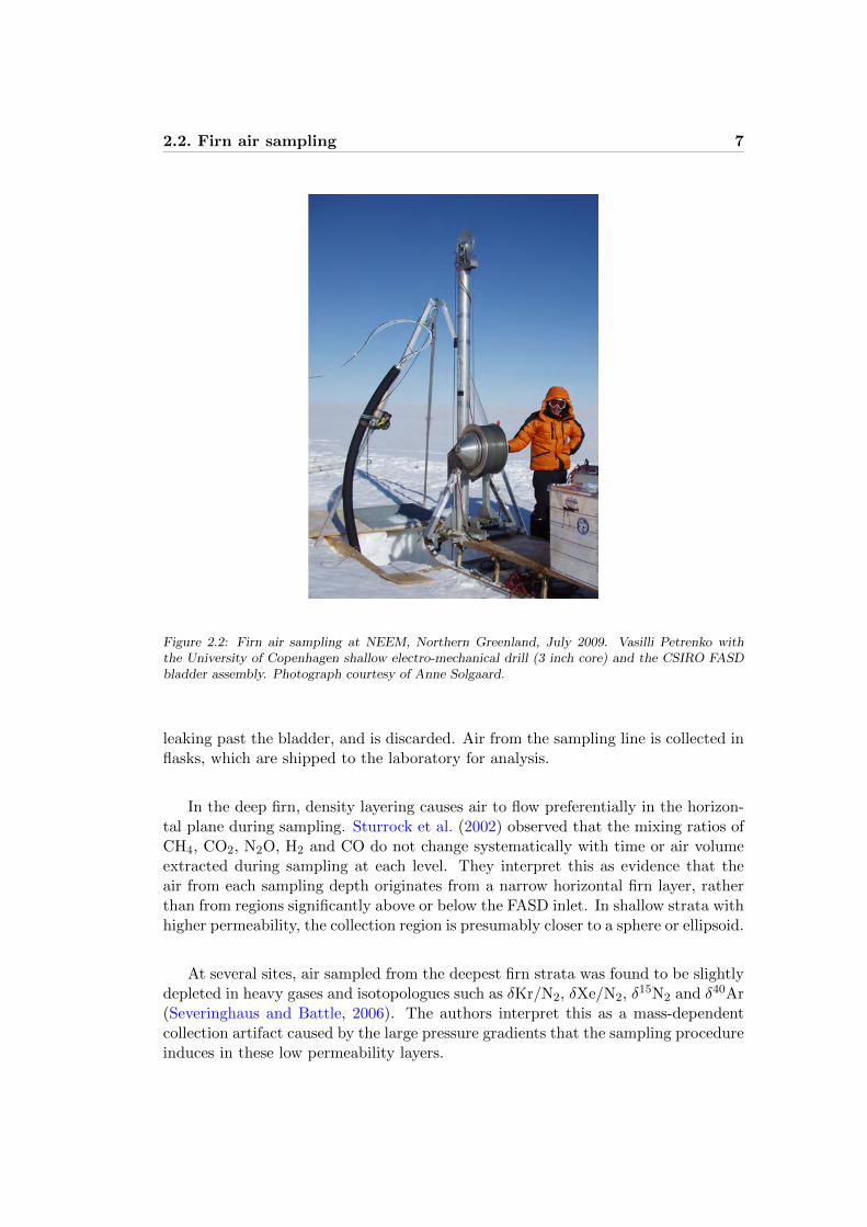
Figure 2.2: Firn air sampling at NEEM, Northern Greenland, July 2009. Vasilli Petrenko withthe University of Copenhagen shallow electro-mechanical drill (3 inch core) and the CSIRO FASDbladder assembly. Photograph courtesy of Anne Solgaard.

leaking past the bladder, and is discarded. Air from the sampling line is collected inflasks, which are shipped to the laboratory for analysis.

In the deep firn, density layering causes air to flow preferentially in the horizon-tal plane during sampling. Sturrock et al. (2002) observed that the mixing ratios ofCH4, CO2, N2O, H2 and CO do not change systematically with time or air volumeextracted during sampling at each level. They interpret this as evidence that theair from each sampling depth originates from a narrow horizontal firn layer, ratherthan from regions significantly above or below the FASD inlet. In shallow strata withhigher permeability, the collection region is presumably closer to a sphere or ellipsoid.

At several sites, air sampled from the deepest firn strata was found to be slightlydepleted in heavy gases and isotopologues such as δKr/N2, δXe/N2, δ15N2 and δ40Ar(Severinghaus and Battle, 2006). The authors interpret this as a mass-dependentcollection artifact caused by the large pressure gradients that the sampling procedureinduces in these low permeability layers.

8 Chapter 2. Overview of firn air studies

Table

2.1

:O

verv

iewof

firn

air

sam

plin

gsites

and

chara

cteristics.

Site

Loca

tion

Altitu

de

pT

AC

Zd

epth

zcod

Yea

r(s)M

ain

reference

(ma.s.l.)

(hP

a)

( ◦C

)(cm

iceyr −

1)

(m)

(m)

sam

pled

North

ernh

emisp

here

Dev

on

Isl.75.3◦N

82.1◦W

1929

792a

-23

30

∼0b

59

1998

FIR

ET

RA

CC

,C

lark

etal.

(2007)

NE

EM

77.4◦N

51.1◦W

2484

745

-28.9

22

478

2008,

2009

Bu

izertet

al.

(2011)

NG

RIP

75.1◦N

42.3◦W

2917

691

-31.1

19

1–2c

78

2001d

CR

YO

ST

AT

,K

aw

am

ura

etal.

(2006)

Su

mm

it72.6◦N

38.4◦W

3214

665

-31.4

23

∼0b

80

1989,

2006

Sch

wan

der

etal.

(1993),

Witra

nt

etal.

(2011)

Sou

thern

hem

isph

ere

Berk

ner

Isl.79.6◦S

45.7◦W

900

895f

-26

13

<2c

64

2003

CR

YO

ST

AT

DE

08-2

66.7◦S

113.2◦E

1250

850

-19

120

0b

85

1993

Eth

eridge

etal.

(1996)

DM

Lg

77.0◦S

10.5◦W

2176

757f

-39

7<

5c

74

1998

FIR

ET

RA

CC

Dom

eC

75.1◦S

123.4◦E

3233

658f

-54

3.2

(2.7c)

2c

100

1999

FIR

ET

RA

CC

Dom

eF

uji

77.3◦S

39.7◦E

3810

600

-57.3

2.8

(2.3c)

9104

1998

Kaw

am

ura

etal.

(2006)

DS

SW

20K

66.8◦S

112.6◦E

1200

850

-21

16

452

1998

Tru

din

ger

(2001)

H72

69.2◦S

41.1◦E

1241

857

-20.3

33

265

1998

Kaw

am

ura

etal.

(2006)

Meg

ad

un

es80.8◦S

124.5◦E

2880

677

-49

∼0h

23

68

2004

Sev

eringh

au

set

al.

(2010)

Sip

leD

om

e81.7◦S

148.8◦W

620

940

-25.4

13

<2b

57

1996,1

998

Sev

eringh

au

set

al.

(2001)

Sou

thP

ole

90.0◦S

2840

681

-51

8<

2b

123

1995–2008j

Sev

eringhau

set

al.

(2001)

Vosto

k78.5◦S

106.8◦E

3471

632

-56

2.4

13b

100

1996

Fab

reet

al.

(2000)

WA

IS-D

79.5◦S

112.1◦W

1766

799f

-31

22

376.5

2005

Battle

etal.

(2011)

YM

85

71.6◦S

40.6◦E

2246

730

-34

17

14k

68

2002

Kaw

am

ura

etal.

(2006)

Un

lessin

dica

tedoth

erwise,

valu

esca

nb

efo

un

din

the

main

reference,

or

references

therein

(last

colu

mn

)a

Hu

ber

etal.

(2006)

bS

everin

gh

au

set

al.

(2010)

cL

an

dais

etal.

(2006)

dT

here

were

two

separa

teN

GR

IPfi

rnair

cam

paig

ns

in2001

(J.

Sch

wan

der,

perso

nal

com

mu

nica

tion

,2011).

fC

alcu

lated

from

the

altitu

de

usin

gth

ep

ressure-a

ltitud

erela

tion

ship

over

Anta

rcticafro

mS

ton

e(2

000).

gA

lsoreferred

toas

BA

Sd

epot

(Lan

dais

etal.,

2006).

Note

that

the

loca

tion

diff

ersfro

mth

at

of

the

ED

ML

iceco

re.h

Th

elo

ng

termavera

ge

accu

mu

latio

nestim

ate

is2.5

cmice

yr −

1.

Sam

plin

gw

as

don

ed

urin

gan

accu

mu

latio

nh

iatu

s.j

Firn

air

was

sam

pled

in1995,

1998,

2001

an

d2008.

kH

igh

win

dsp

eeds

at

this

siteca

use

the

unu

sually

thick

CZ

.

2.3. Physical firn structure and transport properties 9

2.2.2 Overview of firn sampling sites

Firn air has been sampled from sites on both hemispheres, covering a wide rangeof climatic conditions. Table 2.1 gives an overview of sampling sites. The LawDome DE08-2 site is characterised by a very high accumulation rate, which allowsfor reconstructing atmospheric variations with high temporal resolution. At sites onthe Antarctic plateau (Dome C, Dome Fuji, Megadunes, Vostok), on the other hand,the oldest air can be found.

2.3 Physical firn structure and transport properties

2.3.1 Firn density and porosity

Polar firn is a porous medium that is densified gradually under the weight of overlyingprecipitation, until its density ρ approaches the pure ice density ρice of around 920kg m−3. The interstitial space between ice crystals is referred to as the porosity s,which is defined as the volume fraction not occupied by ice, or s = 1− ρ/ρice. It canbe divided into open (sop) and closed (scl) porosity; the former refers to pores thatare still connected to the overlying atmosphere, whereas the latter refers to poresthat have already been closed-off. Owing to firn densification the porosity decreaseswith depth, and air is gradually occluded in bubbles. At Siple station, Schwanderand Stauffer (1984) found that 80% of the bubble volume is formed in the densityrange 795 < ρ < 830 kg m−3. The average density (ρco) at which the bubbles areclosed-off is found in this interval. This mean close-off density was found to beindependent of accumulation rate, and is mostly a function of the site temperature(Martinerie et al., 1992, 1994):

ρco =

(1

ρice+ 6.95 · 10−7T − 4.3 · 10−5

)−1

(2.1)

where T is the mean annual site temperature in K. The mean close-off density in Eq.(2.1) was determined by total air content measurements in mature ice. It is definedthrough the porosity which, at the atmospheric pressure of the site, matches themeasured air content. Apart from temperature, the close-off density (and therebythe total air content) is also influenced by wind strength (Martinerie et al., 1994)and insolation (Raynaud et al., 2007).

A second useful definition is the full close-off depth zcod (with correspondingρcod), which is the depth where all air is occluded (sop = 0). The full close-off isdeeper than the mean close-off depth of Eq. (2.1). The deepest point at which firnair can be sampled in the field is around zcod.

Several scl parameterizations exist. Schwander (1989) gives the following em-pirical relation based on measurements of bubble volume in ice samples from Siplestation, Antarctica:

10 Chapter 2. Overview of firn air studies

0 0.1 0.2 0.390

80

70

60

50

40

30

20

10

0

Lock−in depth

Close−off depth

Lock−In Zone

DiffusiveZone

Convective Zone

δ15N−N2 (‰)

0 0.2 0.4 0.6

Velocity (m yr−1)

400 600 800

Density (kg m−3)

0 2 4 6 890

80

70

60

50

40

30

20

10

0

Dep

th (

m)

Porosity (m3 m−3) × 10−2

wair

wice

sop

scl

a) b) c)

Figure 2.3: Firn characteristics at NEEM. a) Firn density and porosity using the parameterizationsof Schwander (1989) (solid line) and Goujon et al. (2003) (dashed line). b) Downward velocity offirn layers (wice) and of air in the open porosity wair) calculated using Eq. (2.4). c) Zonal divisionbased on gravitational enrichment of δ15N-N2. Data are corrected for thermal fractionation.

scl =

{s exp [75(ρ/ρcod − 1)] for ρ ≤ ρcod

s for ρ > ρcod(2.2)

It must be noted that measurements of bubble volume tend to underestimate closedporosity, as pores can be re-opened by sample cutting. (Severinghaus and Battle,2006) adapted Eq. (2.2) for Summit, Greenland, to have a more gradual close-off.

An alternative parameterization is given by Goujon et al. (2003), based on densityand total air content measurements from three Greenland and Antarctic sites:

scl = 0.37s

(s

sco

)−7.6 (2.3)

where sco is the mean close-off porosity sco = 1−ρco/ρice. Equation (2.3) is designedto be consistent with Eq. (2.1), and indicates that 37 % of the porosity is closed forρco. Both parameterizations are shown in Figure 2.3a.

2.3. Physical firn structure and transport properties 11

2.3.2 Open porosity air flow and transport properties

In the firn-ice transition air bubbles are trapped and advected downwards with theice. Conservation of mass demands an air flow in the open pores to replace the airthus removed. Assuming the firn to be in steady state with respect to accumulationand densification, the downward velocity of air in the open pores can be derived fromthe porosity ratio and mass conservation (Buizert et al., 2011):

wair =Aρice

s∗opp0

(scl(zCOD)pcl(zCOD)

ρCOD− scl(z)pcl(z)

ρ(z)

)(2.4)

where A is the accumulation rate in m yr−1 ice equivalent, s∗op the effective openporosity s∗op = sop exp(Mairgz/RT ), p0 the barometric pressure, pcl(z) the enhancedpressure in closed bubbles due to firn compaction, Mair the molar mass of air inkg mol−1, g the gravitational acceleration and R the molar gas constant. The re-sult is plotted in Figure 2.3b, together with the downward velocity of the ice layerswice = Aρice/ρ. The ice layers descend faster than the air does; i.e. the air in theopen porosity is moving upwards relative to the ice matrix. This back flow is due tocompression of open pores by the firn densification process (Rommelaere et al., 1997).

Pore geometry and connectivity dictate the firn air transport properties. Gasdiffusivity and permeability in firn samples have been determined using direct mea-surements (Albert et al., 2000; Fabre et al., 2000; Schwander et al., 1988), and bymodeling of gas transport in reconstructed pore geometries (Courville et al., 2011;Freitag et al., 2002). However, gas diffusivities determined on individual firn samplesdo not represent the transport properties of the firn as a whole (Fabre et al., 2000),showing that the lateral dimensions of the diffusive path exceed that of a typical firnsample.

2.3.3 Density layering

Polar firn is a layered medium that exhibits large density variations around the meancaused by seasonal changes in climatic conditions and precipitation density, as wellas wind and insolation features that are preserved in the densification process. Ashigh-density layers reach the close-off density first, they can form impermeable layersthat inhibit vertical gas transport (Martinerie et al., 1992). Such sealing layers areoften invoked to explain the presence of a non-diffusive zone, or lock-in zone (LIZ)just above the bubble close-off depth (Battle et al., 1996; Landais et al., 2006). Firnair can be pumped from the LIZ, meaning a large (laterally) connected open porositystill exists in the low density layers.

The high density sealing layers have been linked to winter precipitation throughmeasurements of water stable isotopes (Martinerie et al., 1992). Recent studies offirn microstructure indicate a density cross-over around 600-650 kg m−3, suggesting

12 Chapter 2. Overview of firn air studies

that high density LIZ layers originate as low density layers at the surface (Freitaget al., 2004). Boreholes separated by as little as 65 m were found to have differ-ent firn air transport properties caused by lateral variability in the firn stratigraphy(Buizert et al., 2011).

Although the dense layers impede vertical transport, they do not completely sealoff the air below. The air content implied by such fully sealing layers is incompatiblewith measurements in mature ice. Furthermore, at many sites firn air transportmodels require finite gas diffusivity in the LIZ to reproduce the measured mixingratios of trace gases (Severinghaus et al., 2010; Witrant et al., 2011). The back flowof air due to pore compression can be facilitated by (micro) cracks and channels inthe dense layers.

2.4 Trace gas transport in the firn

2.4.1 Zonal description of transport

The firn column is commonly divided into three zones, based on the gravitationalisotopic enrichment of molecular nitrogen with depth (Sowers et al., 1992). Thezones correspond to different modes of firn air transport, as depicted in Fig. 2.3c.The convective zone (CZ) refers to the upper few meters of the firn column which arevigorously ventilated. The air in the CZ is essentially of current atmospheric com-position, and consequently it has the same δ15N-N2 as the atmosphere (which is zeroby definition). Below the CZ we find the diffusive zone (DZ), where mass transferis dominated by molecular diffusion. In diffusive equilibrium gravitational separa-tion gives enrichment in heavy isotopes with depth, as is evident from the presentedδ15N-N2 measurements. The lock-in depth is defined as the depth at which gravita-tional enrichment stops. Continued pore compaction leads to a decreasing effectivediffusivity with depth; the lock-in depth corresponds to the point where diffusivitybecomes effectively zero. At this depth the air gets isolated from the atmosphere,and therefore the lock-in depth determines the age in mature ice. Below the lock-indepth we find the lock-in zone (LIZ), or non-diffusive zone, where advection with theice matrix dominates the transport. Since advection does not discriminate betweenisotopologues, gravitational separation does not occur in the LIZ. The existence ofthe LIZ has been linked to the formation of high density sealing layers that inhibitvertical diffusion (section 2.3.3).

2.4.2 Overview of mass transfer mechanisms

2.4.2.1 Diffusion

Spatial variations in gas concentration or partial pressure lead to isobaric mass trans-fer along the gradient, from regions of higher to lower concentration. In porousmedia, such as polar firn or unsaturated soil, two types of diffusion should be con-sidered. Knudsen diffusion occurs when the pore diameter is sufficiently small, or

2.4. Trace gas transport in the firn 13

pressure sufficiently low, and molecules collide predominately with the walls ratherthan with other gas molecules. The second type is molecular diffusion, which rep-resents the opposite regime of predominantly inter-molecular collisions. In polarfirn the molecular free mean path of λ ∼100 nm is about four orders of magnitudesmaller than typical pore sizes of ∼1 mm (Freitag et al., 2004; Kipfstuhl et al., 2009).Consequently, firn air diffusion is of the molecular type. In soils, particle and poresizes are generally much smaller and Knudsen diffusion cannot always be neglected.Fick’s law is commonly used to describe molecular diffusion in firn. The validity ofthis approach has been questioned in the case of soil diffusion (Thorstenson and Pol-lock, 1989), in particular for studies of soil respiration (Freijer and Leffelaar, 1996).When modeling trace gas transport Fick’s law provides a good approximation; it isnot suited to describe transport of main components of air such as O2.

The effective diffusivity of gas X in the open porosity is given by (Dullien, 1975):

DX = sopD0X

τ= sopγX

D0CO2

τ(2.5)

where D0X is the free-air molecular diffusion coefficient for gas X at the pressure and

temperature of the site, τ is the tortuosity of the pore geometry and γX = DX/DCO2

is the diffusivity of gas X relative to that of CO2. Recommended values for γX , aswell as a review of D0

X measurements and their temperature dependence are given inAppendix A. Although parameterizations of τ as a function of sop do exist (Schwan-der et al., 1988), diffusivities measured on firn samples do not represent the diffusivebehaviour of the entire firn (Fabre et al., 2000). Best results are obtained when τ(z) isreconstructed site-specifically using measurements of reference tracers (section 2.5.1).

Diffusive transport leads to a separation of the gas mixture by gravity, resultingin a gradual enrichment in both heavy molecules and isotopologues with depth. Indiffusive equilibrium the enrichment relative to the atmosphere is given in deltanotation by:

δgrav =

[exp

(gz∆M

RT

)− 1

]· 103h ∼=

gz∆M

RT· 103h (2.6)

where ∆M can be the molar mass deviation from air in kg mol−1 (∆M =MX − Mair), or the mass difference between two isotopologues when consideringisotopic enrichment. Macroscopic transport processes, such as convection and ad-vection, can locally drive the air column out of diffusive equilibrium, reducing thegravitational separation below the equilibrium slope given by Eq. (2.6).

Temperature gradients in the firn also lead to diffusive separation of the gasmixture. Thermal diffusion results in seasonal isotope fractionation in the firn inresponse to the annual temperature cycle (Severinghaus et al., 2001; Weiler et al.,2009), as well as isotope excursions in the ice core record during abrupt climate

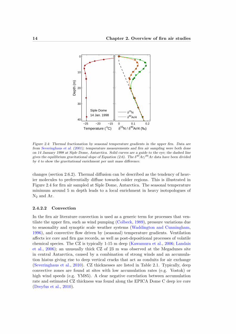
14 Chapter 2. Overview of firn air studies

−25 −20 −1540

30

20

10

0

Temperature ( oC)

Dep

th (

m)

Siple Dome

14 Jan. 1998

0 0.1 0.2

δ15N / δ40Ar/4 (‰)

δ15N

δ40Ar/4

Figure 2.4: Thermal fractionation by seasonal temperature gradients in the upper firn. Data arefrom Severinghaus et al. (2001); temperature measurements and firn air sampling were both doneon 14 January 1998 at Siple Dome, Antarctica. Solid curves are a guide to the eye; the dashed linegives the equilibrium gravitational slope of Equation (2.6). The δ40Ar/36Ar data have been dividedby 4 to show the gravitational enrichment per unit mass difference.

changes (section 2.6.2). Thermal diffusion can be described as the tendency of heav-ier molecules to preferentially diffuse towards colder regions. This is illustrated inFigure 2.4 for firn air sampled at Siple Dome, Antarctica. The seasonal temperatureminimum around 5 m depth leads to a local enrichment in heavy isotopologues ofN2 and Ar.

2.4.2.2 Convection

In the firn air literature convection is used as a generic term for processes that ven-tilate the upper firn, such as wind pumping (Colbeck, 1989), pressure variations dueto seasonality and synoptic scale weather systems (Waddington and Cunningham,1996), and convective flow driven by (seasonal) temperature gradients. Ventilationaffects ice core and firn gas records, as well as post-depositional processes of volatilechemical species. The CZ is typically 1-15 m deep (Kawamura et al., 2006; Landaiset al., 2006); an unusually thick CZ of 23 m was observed at the Megadunes sitein central Antarctica, caused by a combination of strong winds and an accumula-tion hiatus giving rise to deep vertical cracks that act as conduits for air exchange(Severinghaus et al., 2010). CZ thicknesses are listed in Table 2.1. Typically, deepconvective zones are found at sites with low accumulation rates (e.g. Vostok) orhigh wind speeds (e.g. YM85). A clear negative correlation between accumulationrate and estimated CZ thickness was found along the EPICA Dome C deep ice core(Dreyfus et al., 2010).

2.4. Trace gas transport in the firn 15

The CZ thickness can be determined empirically using the barometric line fittingmethod (Bender et al., 1994), in which the barometric slope is fit to isotopic datain the lower DZ, where the gravitational separation is undisturbed by temperaturegradients and ventilation. The intercept with the depth-axis gives the CZ thickness,as shown in Figures 2.3c and 2.4.

In numerical modeling of firn air transport, convection can be included in severalways. The most rudimentary way is to use the bottom of the CZ as the upperboundary, and assume the air above to be of atmospheric composition. A moreadvanced approach is to include an eddy diffusion term that equally affects all gasesand isotopologues (Kawamura et al., 2006):

Deddy(z) = D0eddy exp

(− z

H

)(2.7)

where D0eddy is the eddy diffusivity at the surface and H is a characteristic depth

scale. The eddy diffusion terms prevents gravitational separation by overwhelmingmolecular diffusion.

2.4.2.3 Advection

The bulk motion of air in the open porosity (section 2.3.2) gives rise to downwardadvective mass transfer of trace gases. Firn air models deal with advection in differentways. It can be included by dividing the firn column into boxes of equal air content,and shuffling them downwards after a given time interval has elapsed (Schwanderet al., 1993). An advantage of this approach is that it minimizes numerical diffusionartifacts. Alternatively, advection can be included as a continuous flux using acalculated air velocity in the open pores (Rommelaere et al., 1997; Sugawara et al.,2003). A third approach is to work in a Lagrangian reference frame that movesdownwards with descending ice layers (Trudinger et al., 1997). It must be notedthat this approach overestimates the advective transport, unless the backflow due topore compaction is explicitly taken into account.

2.4.2.4 Dispersive mixing

Equation (2.4) describes the average air velocity; in reality a non-uniform velocitydistribution exists between air expelled upwards by pore compaction, and air inisolated pockets which is advected downwards at the velocity of descending ice layers.Furthermore, atmospheric pressure variations and firn densification induce pressuregradients in the firn, which force viscous air flow. All these macroscopic flow patternslead to dispersive mixing throughout the firn column, although it is overwhelmedby molecular diffusion in the DZ. Soil air studies have shown that viscous flow fromatmospheric pressure fluctuations can induce mixing down to tens of meters, andthat the dispersive flux can exceed the diffusive one (Massmann and Farrier, 1992).Firn air models do not explicitly include these flow patterns, and dispersive mixing

16 Chapter 2. Overview of firn air studies

300 320 340 360 380

120

100

80

60

40

20

0

CO2 (ppm)

NEEM 2008

South Pole 1995

0 2 4 6 80

0.1

0.2

0.3

0.4

0.5

0.6

Age (yr)

South Pole 25 m 30 m 40 m 60 m 80 m100 m

0 50 100 150 2000

1

2

3

4

Age (yr)

NEEM

South Pole

×10−2

Dep

th (

m)

Age

dis

trib

utio

n G

(yr

−1 )

Age

dis

trib

utio

n G

(yr

−1 )

a)

b)

c)

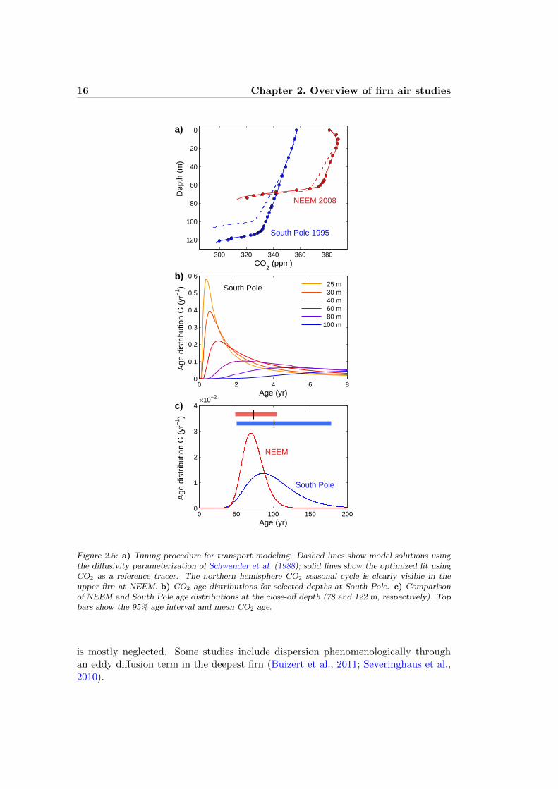
Figure 2.5: a) Tuning procedure for transport modeling. Dashed lines show model solutions usingthe diffusivity parameterization of Schwander et al. (1988); solid lines show the optimized fit usingCO2 as a reference tracer. The northern hemisphere CO2 seasonal cycle is clearly visible in theupper firn at NEEM. b) CO2 age distributions for selected depths at South Pole. c) Comparisonof NEEM and South Pole age distributions at the close-off depth (78 and 122 m, respectively). Topbars show the 95% age interval and mean CO2 age.

is mostly neglected. Some studies include dispersion phenomenologically throughan eddy diffusion term in the deepest firn (Buizert et al., 2011; Severinghaus et al.,2010).

2.5. Dating of firn air and reconstructing recent atmosphericcomposition 17

2.5 Dating of firn air and reconstructing recent atmo-spheric composition

2.5.1 Reconstructing the effective diffusivity

Numerical firn air transport models are essential for dating and interpretation of firnair records. The largest uncertainty in the transport description is how the effectivediffusivity of gases changes with depth (Eq. 2.5). Best results are obtained when thediffusivity profile is reconstructed through an inverse method (Rommelaere et al.,1997; Trudinger et al., 1997). The method consists of forcing a firn air model with areference tracer of know atmospheric history (usually CO2 or CH4), and optimizingthe fit to the measurements through adjusting the diffusivity profile. The procedureis illustrated in Figure 2.5a for South Pole (SPO) and NEEM. The dashed line showsthe modeled CO2 mixing ratio using the tortuosity parameterization of (Schwanderet al., 1988). The solid lines show the fit to the data after the optimization procedure.

Several studies have used multiple reference tracers simultaneously to improvethe diffusivity reconstruction (Buizert et al., 2011; Trudinger et al., 2002).

2.5.2 Age distribution

Firn air does not have a single age, but is a mixture of air with different ages. Figure2.5b shows for SPO how the CO2 age distribution G(z, t) progresses with depth. Themean age Γ(z) of the gas mixture (first moment of the distribution) increases withdepth, as the gases need time to be transported into the firn. Diffusion broadensthe distribution with depth. Figure 2.5c compares age distributions at the bottomof the firn column for NEEM and SPO. The latter has a longer firn column and lowaccumulation rate, resulting in older air at the bottom of the firn as well as a widerdistribution.

The gas age distribution, which is different for each gas, provides a completedescription of the firn transport properties. Age distributions can be calculated byforcing a numerical firn air transport model at the atmospheric boundary with arectangular pulse of short duration. Alternatively, they have been inferred exper-imentally by measuring the spread of the ∆14C-CO2 “bomb spike” caused by at-mospheric testing of thermonuclear weapons, which peaks in the early to mid 1960s(Levchenko et al., 1996).

The gradual nature of the trapping process further broadens the age distribution.Air bubbles found at a single depth have not all been formed at the same time, andrepresent a mixture of ages. Within the LIZ, where the majority of bubbles form,gas diffusivities are small and air in the open pores is advected downwards at nearlythe same velocity as the ice (Figure 2.3b). Consequently the broadening due totrapping is small compared to the diffusive broadening described above (Blunier andSchwander, 2000).

18 Chapter 2. Overview of firn air studies

0 20 40 60 80 100

Age (yr)

−4 −2 0 2

120

100

80

60

40

20

0

δ18O−CO2 (‰ vs. PDB)

Dep

th (

m)

South Pole 2001

δ18Oeq

T1/2

= −37 ‰

= 371 yr

Figure 2.6: Oxygen exchange between CO2 and firn results in 18O depletion with depth (lower axis).The dashed line shows the expected δ18O signal in the absence of exchange; the solid line gives thebest fit to the data based on the modeled ages (grey curve, upper axis) and the parameters listed.The reaction half-time t1/2 is the only parameter which is tuned in the data fitting.

2.5.3 Firn air dating with δ18O of CO2

An alternative firn air dating method based on the isotopic composition of CO2 hasbeen presented by Clark et al. (2007). Atmospheric δ18O-CO2 is relatively stableover time (Allison and Francey, 2007). Within the firn, atomic oxygen exchangewith water molecules gradually alters the oxygen isotopic composition of CO2, untilequilibrium with the strongly depleted δ18O of glacial ice is reached (Siegenthaleret al., 1988). This principle is illustrated in Figure 2.6 for SPO firn.

Depending on the site temperature, the time required for the magnitude of theexchange to reach half its final magnitude (t1/2) ranges from tens to hundreds of yearsdepending on temperature (Assonov et al., 2005). Knowing the rate of O-exchange,the amount of time the CO2 has been in contact with the ice (i.e. the age) can becalculated. The main advantage of the technique is its applicability to warm siteswith summer melt layers that complicate conventional dating. The drawback is thatt1/2 and the equilibrium fractionation must be well known. Clark et al. (2007) solvethis issue by using the ∆14C-CO2 signal, which peaks around 1963, as an absoluteage marker to calibrate t1/2.

2.6. Effects of firn air transport on ice core and firn gas records 19

2.5.4 Reconstructing recent atmospheric composition

The firn air itself preserves a continuous record of atmospheric composition whichcan be sampled to reconstruct trace gas mixing ratios and isotopes for the recentatmosphere. Each firn air sample represents a mixture of gas ages, and consequentlymixing ratios measured in the firn cannot be directly mapped onto a timescale.

Once the firn air transport is well characterized using reference tracers, the for-ward diffusive problem is well described by the modeled age distribution alone. Sub-sequently the most probable atmospheric history of a trace gas of interest can bereconstructed from firn air measurements through an inverse method (Rommelaereet al., 1997; Sugawara et al., 2003; Trudinger et al., 2002). For a more rudimentarydating, mixing ratios of a trace gas of interest can also be directly compared to ref-erence gas measurements at identical sampling depths (Montzka et al., 2004).

Firn air has thus been used to reconstruct the recent atmospheric mixing ratiosand/or isotopic composition of e.g. carbon dioxide (e.g. Etheridge et al., 1996),methane (e.g. Braunlich et al., 2001), ethane (Aydin et al., 2011), nitrous oxide (e.g.Ishijima et al., 2007), carbon monoxide (Assonov et al., 2007), several halocarbons(e.g. Butler et al., 1999; Sturges et al., 2001a) and carbonyl sulfide (e.g. Sturgeset al., 2001b).

2.6 Effects of firn air transport on ice core and firn gasrecords

The firn layer complicates the interpretation of ice core records, as it alters theatmospheric composition prior to bubble closure. At the same time the peculiaritiesof firn air transport give rise to additional signals which can be used for datingand climate reconstruction. In this section we discuss the consequences of firn airtransport for the interpretation of ice core and firn air records.

2.6.1 Delta age and gravitational fractionation

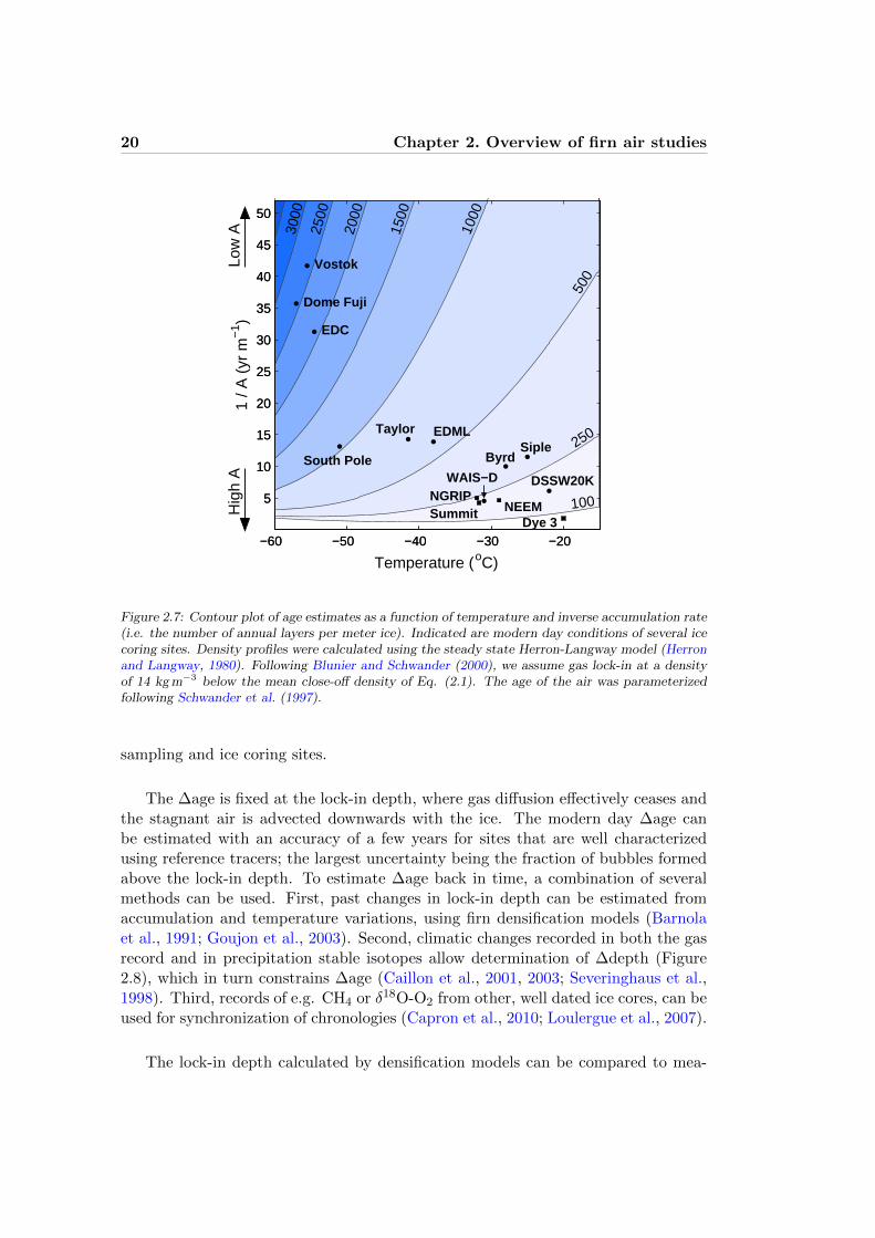
Continued exchange with the atmosphere keeps firn air at the lock-in depth youngerthan the surrounding ice, resulting in an age difference ∆age between glacial ice andthe air bubbles it contains (Schwander and Stauffer, 1984). This is arguably themost important artifact of the firn layer. Accurate ∆age estimates are pivotal ininvestigating the relative timing of abrupt changes in temperature and greenhousegas concentrations (Barnola et al., 1991; Fischer et al., 1999), inter-hemispheric syn-chronization of ice core records (Blunier and Brook, 2001; Morgan et al., 2002) andderiving consistent ice core timescales (Lemieux-Dudon et al., 2010). Figure 2.7shows age estimates as a function of accumulation rate and temperature, assumingstationary conditions. The figure also indicates modern day conditions of several firn

20 Chapter 2. Overview of firn air studies

−60 −50 −40 −30 −20

5

10

15

20

25

30

35

40

45

50

100

250

500

1000

1500

2000

2500

3000

Dome Fuji

Vostok

EDC

South Pole

EDML

DSSW20K

TaylorSiple

Byrd

WAIS−D

Dye 3NEEM

NGRIPSummit

Temperature ( oC)

1 / A

(yr

m−

1 )Lo

w A

Hig

h A

−60 −50 −40 −30 −20

5

10

15

20

25

30

35

40

45

50

Figure 2.7: Contour plot of age estimates as a function of temperature and inverse accumulation rate(i.e. the number of annual layers per meter ice). Indicated are modern day conditions of several icecoring sites. Density profiles were calculated using the steady state Herron-Langway model (Herronand Langway, 1980). Following Blunier and Schwander (2000), we assume gas lock-in at a densityof 14 kg m−3 below the mean close-off density of Eq. (2.1). The age of the air was parameterizedfollowing Schwander et al. (1997).

sampling and ice coring sites.

The ∆age is fixed at the lock-in depth, where gas diffusion effectively ceases andthe stagnant air is advected downwards with the ice. The modern day ∆age canbe estimated with an accuracy of a few years for sites that are well characterizedusing reference tracers; the largest uncertainty being the fraction of bubbles formedabove the lock-in depth. To estimate ∆age back in time, a combination of severalmethods can be used. First, past changes in lock-in depth can be estimated fromaccumulation and temperature variations, using firn densification models (Barnolaet al., 1991; Goujon et al., 2003). Second, climatic changes recorded in both the gasrecord and in precipitation stable isotopes allow determination of ∆depth (Figure2.8), which in turn constrains ∆age (Caillon et al., 2001, 2003; Severinghaus et al.,1998). Third, records of e.g. CH4 or δ18O-O2 from other, well dated ice cores, can beused for synchronization of chronologies (Capron et al., 2010; Loulergue et al., 2007).

The lock-in depth calculated by densification models can be compared to mea-

2.6. Effects of firn air transport on ice core and firn gas records 21

surements of the gravitational enrichment in δ15N-N2, which records the diffusivecolumn length. Note that the diffusive column length does not directly give thelock-in depth, as the thickness of the CZ is unknown. Models predict a deeper lock-in depth during colder glacial conditions, implying a larger δ15N-N2. This is indeedobserved in Greenland ice cores (Schwander et al., 1997). Antarctic ice cores (withthe exception of the coastal Byrd site) show a pronounced model-data mismatchwith lower δ15N-N2 (i.e. shorter diffusive column) during glacial conditions (Landaiset al., 2006). An increased CZ thickness is often invoked to explain the mismatch,where the Megadunes site, with an unusually thick convective zone of > 23 m, couldprovide a modern analog for central Antarctic glacial conditions (Severinghaus et al.,2010).

Measurements of gravitational enrichment in δ15N-N2 are also used to correctgas records for the effect of gravity.

2.6.2 Thermal fractionation and gas thermometry

Thermal diffusion causes isotopic fractionation in the presence of temperature gra-dients (section 2.4.2.1). Seasonal temperature variations and the associated isotopeeffect occur only in the upper firn (Figure 2.4). They could potentially affect thedeep firn (and thereby the ice core record) through seasonality in transport prop-erties, such as convective mixing and temperature dependent diffusion coefficients.No evidence for such rectifier effects was found (Severinghaus et al., 2001); seasonalthermal fractionation should have little or no impact on the ice core record.

Climate-induced changes in mean annual surface temperature, on the other hand,can cause isotopic signals in the ice core record if the temperature change is suffi-ciently large and rapid. This principle is illustrated in Fig 2.8 for the GISP2 core incentral Greenland. Abrupt warming events during the last deglaciation are accom-panied by positive δ15N and δ40Ar excursions as the deep, colder firn gets enrichedin heavy isotopes relative to the warmer surface. As the temperature sensitivityof δ15N and δ40Ar/4 is different, the signals can be used in combination to inferthe amplitude of the temperature change (Landais et al., 2004; Leuenberger et al.,1999; Severinghaus and Brook, 1999). The excursions furthermore provide clear timemarkers in the gas record that can be used to determine ∆age more accurately thandensification models allow. The method does not work well for Antarctica wheretemperature changes are more gradual.

2.6.3 Molecular size fractionation at close-off

Within the LIZ a systematic enrichment is observed for gas species with a smallmolecular diameter, such as He, Ar, Ne and O2 (Huber et al., 2006; Severinghaus andBattle, 2006). This has been explained by the preferential exclusion of these speciesfrom closing bubbles, causing them to accumulate in the open porosity. Closed bub-bles are pressurized through continued firn compaction, which increases gas partial

22 Chapter 2. Overview of firn air studies

Δdepth Δdepth

YD B−A

−42

−40

−38

−36

−34

δ

18O

(‰

)

1650 1700 1750 1800 18500.3

0.4

0.5

0.6

0.7

Depth (m)

δ15N

, (‰)

δ40A

r/4

Figure 2.8: GISP2 oxygen isotopes of precipitation with 200-yr running average (upper curve,left axis) and transient thermal fractionation signals in N2 and Ar caused by rapid warming overGreenland (lower data, right axis). Data from (Severinghaus et al., 1998) and (Severinghaus andBrook, 1999). The depth difference between the observed warming in the ice and gas recordsconstrains ∆age.

pressures in the bubbles relative to the open porosity. This gradient drives selec-tive permeation of gas through the ice lattice. Huber et al. (2006) find a strongdependence of the fractionation magnitude on the collision diameter of the molecule,suggesting a critical size of 3.6 A. Recently Battle et al. (2011) reported that the O2

excluded from the closing bubbles is isotopically depleted in δ18O-O2, showing thepermeation through the ice lattice to be mass dependent. The mechanisms causingclose-off fractionation are similar to those responsible for post-coring gas loss duringice sample storage (Bender et al., 1995).

The close-off fractionation is shown in Figure 2.9 for SPO firn. The enrichmentis strongest in the LIZ where the vast majority of bubbles are occluded, and thelow effective diffusivity prevents diffusion of the signal. Note that a gradient existsin the DZ, indicative of an upward diffusive gas flux. Hereby some O2 (Ne) is lostto the atmosphere, leading to a correspondingly depleted δO2/N2 (δNe/N2) in gasbubbles.

It has been found that δO2/N2 can be used as a local summer insolation proxy,allowing orbital tuning of ice core chronologies (Bender, 2002; Kawamura et al.,

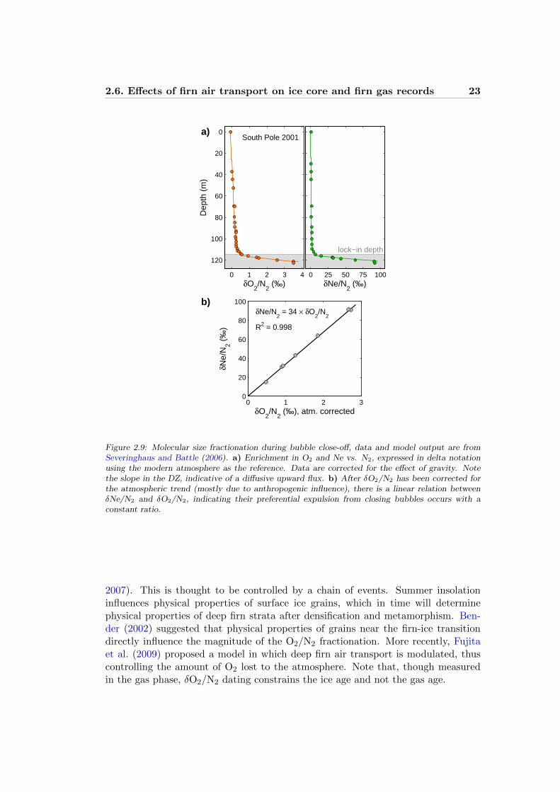
2.6. Effects of firn air transport on ice core and firn gas records 23

South Pole 2001

0 1 2 3 4

120

100

80

60

40

20

0

δO2/N

2 (‰)

Dep

th (

m)

lock−in depth

0 25 50 75 100δNe/N

2 (‰)

0 1 2 30

20

40

60

80

100

δNe/

N2 (

‰)

δO2/N

2 (‰), atm. corrected

δNe/N2 = 34 × δO

2/N

2

R2 = 0.998

a)

b)

Figure 2.9: Molecular size fractionation during bubble close-off, data and model output are fromSeveringhaus and Battle (2006). a) Enrichment in O2 and Ne vs. N2, expressed in delta notationusing the modern atmosphere as the reference. Data are corrected for the effect of gravity. Notethe slope in the DZ, indicative of a diffusive upward flux. b) After δO2/N2 has been corrected forthe atmospheric trend (mostly due to anthropogenic influence), there is a linear relation betweenδNe/N2 and δO2/N2, indicating their preferential expulsion from closing bubbles occurs with aconstant ratio.

2007). This is thought to be controlled by a chain of events. Summer insolationinfluences physical properties of surface ice grains, which in time will determinephysical properties of deep firn strata after densification and metamorphism. Ben-der (2002) suggested that physical properties of grains near the firn-ice transitiondirectly influence the magnitude of the O2/N2 fractionation. More recently, Fujitaet al. (2009) proposed a model in which deep firn air transport is modulated, thuscontrolling the amount of O2 lost to the atmosphere. Note that, though measuredin the gas phase, δO2/N2 dating constrains the ice age and not the gas age.

24 Chapter 2. Overview of firn air studies

LIZDZ

−0.15 −0.1 −0.05 0

70

60

50

40

30

20

10

0

εDF

/ δ13CO2 (‰)

Dep

th (

m)

CICCSIROINSTAARLGGE−GIPSAOSUSIOEquation (8)

Figure 2.10: Isotopic diffusive fractionation in the NEEM firn for a hypothetical atmospheric CO2

scenario. See Buizert et al. (2011) for details and model acronyms.

2.6.4 Isotopic diffusive fractionation

A secular variation in the atmospheric mixing ratio of a gas species results in isotopicfractionation in the firn, even in the absence of a changing atmospheric isotopic com-position (Trudinger et al., 1997). As an example, consider a rise in atmospheric CO2.The lighter 12CO2 isotopologue diffuses faster into the firn than 13CO2, giving rise toisotopic depletion with depth. This diffusive fractionation εDF can be approximatedby

εDF =

{kC

(DiDj− 1)

Γ(z) for z ≤ zlid

εDF(zlid) for z > zlid

(2.8)

where C is the atmospheric mixing ratio (ppm), k the rate of increase (ppm yr−1),Di (Dj) the diffusion coefficient of the minor (major) isotopologue, Γ(z) the meangas age (yr), and zlid the lock-in depth.

Figure 2.10 shows the diffusive fractionation calculated with Eq. (2.8) and six nu-merical firn air models for a hypothetical exponential CO2 increase of k/C = 2.5·10−3

(equivalent to k = 1 ppm yr−1 at C = 400 ppm), while keeping δ13CO2 fixed at 0h. Within the DZ, the profiles agree well. Within the LIZ the model solutionsdiverge, as the models use different parameterizations of LIZ transport. More workis needed to elucidate the nature of LIZ transport, and thereby the true magnitudeof the diffusive fractionation.

2.7. Summary 25

Firn air and ice core records need to be corrected for the effect of diffusive frac-tionation, although often the effect will be small. Some corrections for the recent an-thropogenic increase found in literature are 0.1 hfor δ13CO2 at Law Dome (Franceyet al., 1999) and 1.2 hfor δ13CH4 at WAIS-Divide (Mischler et al., 2009). The ef-fect is larger for CH4 as the relative mass difference between the isotopologues, andthereby the ratio of diffusivities, is larger.

2.6.5 Smoothing by diffusion and bubble trapping

The firn causes smoothing of the atmospheric signal, limiting the temporal resolu-tion at which atmospheric variations are recorded in the ice. One can think of thefirn as a low-pass filter to the atmospheric signal; high frequency variations, such asthe annual cycles of trace gases, are not preserved. Spahni et al. (2003) studied theattenuation of the rapid CH4 excursion associated with the 8.2 kyr event, and foundit to be attenuated by about 13% in the GRIP core, and 44% in the EPICA DomeC core. The low accumulation rate and deeper lock-in depth at the latter site areresponsible for the stronger attenuation.

By taking the Fourier transform of the age distribution, we can evaluate howatmospheric variations at different time scales are attenuated by the firn column(Figure 2.11). As the bubble trapping occurs predominately throughout the LIZ,the age distribution halfway the LIZ is taken as a measure of the signal recordedin the air bubbles. Additional smoothing by the trapping process is not accountedfor. Atmospheric variations on time scales of several hundreds of years or longer arerecorded with their full amplitude; variations faster than ∼50 years are attenuatedso strongly they cannot be observed within the measurement noise. Variations atintermediate time scales (such as the aforementioned 8.2 kyr event) are recorded withreduced amplitude. In theory, the true atmospheric history could be reconstructedfrom high resolution records with deconvolution techniques also used for water stableisotope records (Johnsen, 1977).

2.7 Summary

Firn air studies are important for interpretation of ice core gas records and recon-structing recent atmospheric variations. Following δ15N-N2 gravitational enrichment,the firn column is divided in the convective, diffusive and lock-in zones, where gastransport is dominated by surface ventilation, diffusion and advection, respectively.Transport properties are determined by pore geometry and connectivity, as well asdensity layering. Diffusivity measurements on finite samples do not represent theentire firn, and diffusivity needs to be reconstructed using reference tracers. Grav-itational separation, ∆age, diffusive smoothing and diffusive isotopic fractionationare firn effects that need to be considered when interpreting ice core records. Ther-mal fractionation and close-off fractionation give rise to new proxies that can be used

26 Chapter 2. Overview of firn air studies

NEEM

South Pole

101

102

103

10−6

10−4

10−2

100

101

102

103

0

0.5

1

Period (yr)

Sig

nal a

mpl

itude

Sig

nal a

mpl

itude

a)

b)

Figure 2.11: Bode plot of the firn transfer function on a) a log-log scale and b) a semi-log scale,obtained by fast Fourier transform (FFT) of the modeled CO2 age distributions halfway the LIZ.The transmitted signal amplitude is plotted as a function of the period of the oscillation (P = 1/fwith f the frequency in yr−1).

for temperature reconstruction and dating.

2.8 References

Albert, M. R., Schultz, E. F., and Perron, F. E. J. (2000). Snow and firn permeability at siple dome,antarctica. Ann. Glaciol., 31:353–356.

Allison, C. E. and Francey, R. J. (2007). Verifying southern hemisphere trends in atmosphericcarbon dioxide stable isotopes. J. Geophys. Res.-Atm, 112(D21):27. ISI Document Delivery No.:228CQ Times Cited: 5 Cited Reference Count: 62 Allison, C. E. Francey, R. J.

Assonov, S. S., Brenninkmeijer, C. A. M., and Jockel, P. (2005). The o-18 isotope exchange rate be-tween firn air co2 and the firn matrix at three antarctic sites. J. Geophys. Res.-Atm, 110(D18):15.

Assonov, S. S., Brenninkmeijer, C. A. M., Jockel, P. J., Mulvaney, R., Bernard, S., and Chappellaz,J. (2007). Evidence for a co increase in the sh during the 20th century based on firn air samplesfrom berkner island, antarctica. Atmos. Chem. Phys., 7:295–308.

Aydin, M., Verhulst, K. R., Saltzman, E. S., Battle, M. O., Montzka, S. A., Blake, D. R., Tang,Q., and Prather, M. J. (2011). Recent decreases in fossil-fuel emissions of ethane and methanederived from firn air. Nature, 476(7359):198–201.

Barnola, J. M., Pimienta, P., Raynaud, D., and Korotkevich, Y. S. (1991). Co2-climate relationshipas deduced from the vostok ice core - a reexamination based on new measurements and on areevaluation of the air dating. Tellus B, 43(2):83–90. ISI Document Delivery No.: FG714 TimesCited: 119 Cited Reference Count: 0.

2.8. References 27

Battle, M., Bender, M., Sowers, T., Tans, P. P., Butler, J. H., Elkins, J. W., Ellis, J. T., Conway,T., Zhang, N., Lang, P., and Clarket, A. D. (1996). Atmospheric gas concentrations over the pastcentury measured in air from firn at the south pole. Nature, 383(6597):231–235.

Battle, M. O., Severinghaus, J. P., Sofen, E. D., Plotkin, D., Orsi, A. J., Aydin, M., Montzka, S. A.,Sowers, T., and Tans, P. P. (2011). Controls on the movement and composition of firn air at thewest antarctic ice sheet divide. Atmos. Chem. Phys. Discuss., 11(6):18633–18675.

Bender, M., Sowers, T., and Lipenkov, V. (1995). On the concentrations of o-2, n-2, and ar in trappedgases from ice cores. J. Geophys. Res.-Atm, 100(D9):18651–18660. ISI Document Delivery No.:RV887 Times Cited: 23 Cited Reference Count: 32.

Bender, M. L. (2002). Orbital tuning chronology for the vostok climate record supported by trappedgas composition. Earth Planet Sc. Lett., 204(1-2):275–289. ISI Document Delivery No.: 619LJTimes Cited: 24 Cited Reference Count: 57.

Bender, M. L., Sowers, T., Barnola, J., M, and Chappellaz, J. (1994). Changes in the o2/n2 ratioof the atmosphere during recent decades reflected in the composition of air in the firn at vostokstation, antarctica. Geophys. Res. Lett., 21(3):189–192.

Blunier, T. and Brook, E. J. (2001). Timing of millennial-scale climate change in antarctica andgreenland during the last glacial period. Science, 291(5501):109–112. ISI Document Delivery No.:389VJ Times Cited: 368 Cited Reference Count: 33.

Blunier, T. and Schwander, J. (2000). Gas enclosure in ice: age difference and fractionation, pages307–326. Hokkaido University Press, Sapporo.

Braunlich, M., Aballanin, O., Marik, T., Jockel, P., Brenninkmeijer, C. A. M., Chappellaz, J.,Barnola, J. M., Mulvaney, R., and Sturges, W. T. (2001). Changes in the global atmosphericmethane budget over the last decades inferred from c-13 and d isotopic analysis of antarctic firnair. J. Geophys. Res.-Atm, 106(D17):20465–20481.

Buizert, C., Martinerie, P., Petrenko, V. V., Severinghaus, J. P., Trudinger, C. M., Witrant, E.,Rosen, J. L., Orsi, A. J., Rubino, M., Etheridge, D. M., Steele, L. P., Hogan, C., Laube, J. C.,Sturges, W. T., Levchenko, V. A., Smith, A. M., Levin, I., Conway, T. J., Dlugokencky, E. J.,Lang, P. M., Kawamura, K., Jenk, T. M., White, J. W. C., Sowers, T., Schwander, J., and Blunier,T. (2011). Gas transport in firn: multiple-tracer characterisation and model intercomparison forneem, northern greenland. Atmos. Chem. Phys. Discuss., 11:15975–16021.

Butler, J. H., Battle, M., Bender, M. L., Montzka, S. A., Clarke, A. D., Saltzman, E. S., Sucher,C. M., Severinghaus, J. P., and Elkins, J. W. (1999). A record of atmospheric halocarbons duringthe twentieth century from polar firn air. Nature, 399(6738):749–755.

Caillon, N., Severinghaus, J. P., Barnola, J. M., Chappellaz, J., Jouzel, J., and Parrenin, F. (2001).Estimation of temperature change and of gas age - ice age difference, 108 kyr b.p., at vostok,antarctica. J. Geophys. Res., 106(D23):31893–31901.

Caillon, N., Severinghaus, J. P., Jouzel, J., Barnola, J.-M., Kang, J., and Lipenkov, V. Y. (2003).Timing of atmospheric co2 and antarctic temperature changes across termination iii. Science,299(5613):1728–1731.

Capron, E., Landais, A., Lemieux-Dudon, B., Schilt, A., Masson-Delmotte, V., Buiron, D., Chap-pellaz, J., Dahl-Jensen, D., Johnsen, S., Leuenberger, M., Loulergue, L., and Oerter, H. (2010).Synchronising edml and northgrip ice cores using [delta]18o of atmospheric oxygen ([delta]18oatm)and ch4 measurements over mis5 (80-123 kyr). Quaternary Sci. Rev., 29(1-2):222–234. doi: DOI:10.1016/j.quascirev.2009.07.014.

Clark, I. D., Henderson, L., Chappellaz, J., Fisher, D., Koerner, R., Worthy, D. E. J., Kotzer, T.,Norman, A.-L., and Barnola, J.-M. (2007). Co2 isotopes as tracers of firn air diffusion and agein an arctic ice cap with summer melting, devon island, canada. J. Geophys. Res., 112.

Colbeck, S. C. (1989). Air movement in snow due to windpumping. J. Glaciol., 35(120):209–213.Courville, Z., Horhold, M., Hopkins, M., and Albert, M. (2011). Lattice-boltzmann modeling of the

air permeability of polar firn. J. Geophys. Res., 115(F4):F04032.Craig, H., Horibe, Y., and Sowers, T. (1988). Gravitational separation of gases and isotopes in polar

ice caps. Science, 242(4886):1675–1678.Dreyfus, G. B., Jouzel, J., Bender, M. L., Landais, A., Masson-Delmotte, V., and Leuenberger, M.

(2010). Firn processes and δ15n: potential for a gas-phase climate proxy. Quaternary Sci. Rev.,

28 Chapter 2. Overview of firn air studies

29(1-2):28–42.Dullien, F. A. L. (1975). Single phase flow through porous media and pore structure. The Chemical

Engineering Journal, 10(1):1–34.Etheridge, D. M., Steele, L. P., Langenfelds, R. L., Francey, R. J., Barnola, J. M., and Morgan, V. I.

(1996). Natural and anthropogenic changes in atmospheric co2 over the last 1000 years from airin antarctic ice and firn. J. Geophys. Res., 101(D2):4115–4128.

Fabre, A., Barnola, J. M., Arnaud, L., and Chappellaz, J. (2000). Determination of gas diffusivityin polar firn: Comparison between experimental measurements and inverse modeling. Geophys.Res. Lett., 27(4):557–560.

Fischer, H., Wahlen, M., Smith, J., Mastroianni, D., and Deck, B. (1999). Ice core records ofatmospheric co2 around the last three glacial terminations. Science, 283(5408):1712–1714.

Francey, R., Allison, C., Etheridge, D., Trudinger, C., Enting, I., Leuenberger, M., Langenfelds, R.,Michel, E., and Steele, L. (1999). A 1000-year high precision record of delta C-13 in atmosphericCO2. Tellus B, 51(2):170–193.

Freijer, J. I. and Leffelaar, P. A. (1996). Adapted fick’s law applied to soil respiration. WaterResour. Res., 32(4):791–800.

Freitag, J., Dorbrindt, U., and Kipfstuhl, J. (2002). A new method for predicting transport prop-erties of polar firn with respect to gases on the pore-space scale. Ann. Glaciol., 35:538–544.doi:10.3189/172756402781816582.

Freitag, J., Wilhelms, F., and Kipfstuhl, J. (2004). Microstructure-dependent densi-fication of polar firn derived from x-ray microtomography. J. Glaciol., 50:243–250.doi:10.3189/172756504781830123.

Fujita, S., Okuyama, J., Hori, A., and Hondoh, T. (2009). Metamorphism of stratified firn at domefuji, antarctica: A mechanism for local insolation modulation of gas transport conditions duringbubble close off. J. Geophys. Res., 114.

Goujon, C., Barnola, J. M., and Ritz, C. (2003). Modeling the densification of polar firn includingheat diffusion: Application to close-off characteristics and gas isotopic fractionation for antarcticaand greenland sites. J. Geophys. Res.-Atm, 108(D24):18.

Herron, M. M. and Langway, C. C. (1980). Firn densification - an emperical model. J. Glaciol.,25(93):373–385.

Huber, C., Beyerle, U., Leuenberger, M., Schwander, J., Kipfer, R., Spahni, R., Severinghaus, J. P.,and Weiler, K. (2006). Evidence for molecular size dependent gas fractionation in firn air derivedfrom noble gases, oxygen, and nitrogen measurements. Earth Planet Sc. Lett., 243(1-2):61–73.

Ishijima, K., Sugawara, S., Kawamura, K., Hashida, G., Morimoto, S., Murayama, S., Aoki, S., andNakazawa, T. (2007). Temporal variations of the atmospheric nitrous oxide concentration andits delta n-15 and delta o-18 for the latter half of the 20th century reconstructed from firn airanalyses. J. Geophys. Res.-Atm, 112(D3):12.

Johnsen, S. J. (1977). Stable isotope homogenization of polar firn and ice.Kaspers, K. A., van de Wal, R. S. W., van den Broeke, M. R., Schwander, J., van Lipzig, N. P. M.,

and Brenninkmeijer, C. A. M. (2004). Model calculations of the age of firn air across the antarcticcontinent. Atmos. Chem. Phys., 4(5):1365–1380.

Kawamura, K., Parrenin, F., Lisiecki, L., Uemura, R., Vimeux, F., Severinghaus, J. P., Hutterli,M. A., Nakazawa, T., Aoki, S., Jouzel, J., Raymo, M. E., Matsumoto, K., Nakata, H., Motoyama,H., Fujita, S., Goto-Azuma, K., Fujii, Y., and Watanabe, O. (2007). Northern hemisphere forcingof climatic cycles in antarctica over the past 360,000 years. Nature, 448(7156):912–U4.

Kawamura, K., Severinghaus, J. P., Ishidoya, S., Sugawara, S., Hashida, G., Motoyama, H., Fujii,Y., Aoki, S., and Nakazawa, T. (2006). Convective mixing of air in firn at four polar sites. EarthPlanet Sc. Lett., 244(3-4):672–682.

Kipfstuhl, S., Faria, S. H., Azuma, N., Freitag, J., Hamann, I., Kaufmann, P., Miller, H., Weiler,K., and Wilhelms, F. (2009). Evidence of dynamic recrystallization in polar firn. J. Geophys.Res., 114(B5):B05204.

Landais, A., Barnola, J. M., Kawamura, K., Caillon, N., Delmotte, M., Van Ommen, T., Dreyfus,G., Jouzel, J., Masson-Delmotte, V., Minster, B., Freitag, J., Leuenberger, M., Schwander, J.,Huber, C., Etheridge, D., and Morgan, V. (2006). Firn-air delta n-15 in modern polar sites and

2.8. References 29

glacial-interglacial ice: a model-data mismatch during glacial periods in antarctica? QuaternarySci. Rev., 25(1-2):49–62.

Landais, A., Caillon, N., Goujon, C., Grachev, A. M., Barnola, J. M., Chappellaz, J., Jouzel, J.,Masson-Delmotte, V., and Leuenberger, M. (2004). Quantification of rapid temperature changeduring do event 12 and phasing with methane inferred from air isotopic measurements. EarthPlanet Sc. Lett., 225(1-2):221–232.

Lemieux-Dudon, B., Blayo, E., Petit, J.-R., Waelbroeck, C., Svensson, A., Ritz, C., Barnola, J.-M.,Narcisi, B. M., and Parrenin, F. (2010). Consistent dating for antarctic and greenland ice cores.Quaternary Sci. Rev., 29(1-2):8–20.

Leuenberger, M. C., Lang, C., and Schwander, J. (1999). Delta(15)n measurements as a calibrationtool for the paleothermometer and gas-ice age differences: A case study for the 8200 bp eventon grip ice. J. Geophys. Res.-Atm, 104(D18):22163–22170. ISI Document Delivery No.: 239UZTimes Cited: 40 Cited Reference Count: 37.

Levchenko, V. A., Francey, R. J., Etheridge, D. M., Tuniz, C., Head, J., Morgan, V. I., Lawson, E.,and Jacobsen, G. (1996). The 14c ”bomb spike” determines the age spread and age of co2 in lawdome firn and ice. Geophys. Res. Lett., 23(23):3345–3348.

Loulergue, L., Parrenin, F., Blunier, T., Barnola, J. M., Spahni, R., Schilt, A., Raisbeck, G., andChappellaz, J. (2007). New constraints on the gas age-ice age difference along the epica ice cores,0-50 kyr. Climate of the Past, 3(3):527–540. ISI Document Delivery No.: 215CJ Times Cited:3 Cited Reference Count: 68 Loulergue, L. Parrenin, F. Blunier, T. Barnola, J.-M. Spahni, R.Schilt, A. Raisbeck, G. Chappellaz, J.

Loulergue, L., Schilt, A., Spahni, R., Masson-Delmotte, V., Blunier, T., Lemieux, B., Barnola,J. M., Raynaud, D., Stocker, T. F., and Chappellaz, J. (2008). Orbital and millennial-scalefeatures of atmospheric ch4 over the past 800,000 years. Nature, 453(7193):383–386. ISI DocumentDelivery No.: 301AI Times Cited: 3 Cited Reference Count: 27 Loulergue, Laetitia Schilt, AdrianSpahni, Renato Masson-Delmotte, Valerie Blunier, Thomas Lemieux, Benedicte Barnola, Jean-Marc Raynaud, Dominique Stocker, Thomas F. Chappellaz, Jerome.

Luthi, D., Le Floch, M., Bereiter, B., Blunier, T., Barnola, J.-M., Siegenthaler, U., Raynaud, D.,Jouzel, J., Fischer, H., Kawamura, K., and Stocker, T. F. (2008). High-resolution carbon dioxideconcentration record 650,000-800,000[thinsp]years before present. Nature, 453(7193):379–382.

Martinerie, P., Lipenkov, V. Y., Raynaud, D., Chappellaz, J., Barkov, N. I., and Lorius, C. (1994).Air content paleo record in the vostok ice core (antarctica): A mixed record of climatic andglaciological parameters. J. Geophys. Res., 99:10565–10576.

Martinerie, P., Raynaud, D., Etheridge, D. M., Barnola, J. M., and Mazaudier, D. (1992). Physicaland climatic parameters which influence the air content in polar ice. Earth Planet Sc. Lett.,112(1-4):1–13.

Massmann, J. and Farrier, D. F. (1992). Effects of atmospheric pressures on gas transport in thevadose zone. Water Resour. Res., 28(3):777–791.

Mischler, J. A., Sowers, T. A., Alley, R. B., Battle, M., McConnell, J. R., Mitchell, L., Popp, T.,Sofen, E., and Spencer, M. K. (2009). Carbon and hydrogen isotopic composition of methaneover the last 1000 years. Global Biogeochem. Cy., 23.

Montzka, S. A., Aydin, M., Battle, M., Butler, J. H., Saltzman, E. S., Hall, B. D., Clarke, A. D.,Mondeel, D., and Elkins, J. W. (2004). A 350-year atmospheric history for carbonyl sulfideinferred from antarctic firn air and air trapped in ice. J. Geophys. Res.-Atm, 109(D22):11.

Morgan, V., Delmotte, M., van Ommen, T., Jouzel, J., Chappellaz, J., Woon, S., Masson-Delmotte,V., and Raynaud, D. (2002). Relative timing of deglacial climate events in antarctica and green-land. Science, 297(5588):1862–1864.

Petit, J. R., Jouzel, J., Raynaud, D., Barkov, N. I., Barnola, J. M., Basile, I., Bender, M., Chappel-laz, J., Davis, M., Delaygue, G., Delmotte, M., Kotlyakov, V. M., Legrand, M., Lipenkov, V. Y.,Lorius, C., Pepin, L., Ritz, C., Saltzman, E., and Stievenard, M. (1999). Climate and atmospherichistory of the past 420,000 years from the vostok ice core, antarctica. Nature, 399(6735):429–436.ISI Document Delivery No.: 202TH Times Cited: 1329 Cited Reference Count: 52.

Raynaud, D., Lipenkov, V., Lemieux-Dudon, B., Duval, P., Loutre, M. F., and Lhomme, N. (2007).The local insolation signature of air content in antarctic ice. a new step toward an absolute dating

30 Chapter 2. Overview of firn air studies

of ice records. Earth Planet Sc. Lett., 261(3-4):337–349.Rommelaere, V., Arnaud, L., and Barnola, J. M. (1997). Reconstructing recent atmospheric trace

gas concentrations from polar firn and bubbly ice data by inverse methods. J. Geophys. Res.-Atm,102(D25):30069–30083.

Schwander, J. (1989). The transformation of snow to ice and the occlusion of gases. In Oescher,H. and Langway, C., editors, The Environmental record in glaciers and ice sheets, pages 53–67.John Wiley, New York.

Schwander, J., Barnola, J. M., Andrie, C., Leuenberger, M., Ludin, A., Raynaud, D., and Stauffer,B. (1993). The age of the air in the firn and the ice at summit, greenland. J. Geophys. Res.-Atm,98(D2):2831–2838.

Schwander, J., Sowers, T., Barnola, J. M., Blunier, T., Fuchs, A., and Malaize, B. (1997). Age scaleof the air in the summit ice: Implication for glacial-interglacial temperature change. J. Geophys.Res.-Atm, 102(D16):19483–19493.

Schwander, J. and Stauffer, B. (1984). Age difference between polar ice and the air trapped in itsbubbles. Nature, 311(5981):45–47.

Schwander, J., Stauffer, B., and Sigg, A. (1988). Air mixing in firn and the age of the air at poreclose-off. In Ann. Glaciol., volume 10, pages 141–145.

Severinghaus, J. P., Albert, M. R., Courville, Z. R., Fahnestock, M. A., Kawamura, K., Montzka,S. A., Muhle, J., Scambos, T. A., Shields, E., Shuman, C. A., Suwa, M., Tans, P., and Weiss,R. F. (2010). Deep air convection in the firn at a zero-accumulation site, central antarctica. EarthPlanet Sc. Lett., 293(3-4):359–367.

Severinghaus, J. P. and Battle, M. O. (2006). Fractionation of gases in polar lee during bubbleclose-off: New constraints from firn air ne, kr and xe observations. Earth Planet Sc. Lett., 244(1-2):474–500.

Severinghaus, J. P. and Brook, E. J. (1999). Abrupt climate change at the end of the last glacialperiod inferred from trapped air in polar ice. Science, 286(5441):930–934.

Severinghaus, J. P., Grachev, A., and Battle, M. (2001). Thermal fractionation of air in polar firnby seasonal temperature gradients. Geochem. Geophy. Geosy., 2.

Severinghaus, J. P., Sowers, T., Brook, E. J., Alley, R. B., and Bender, M. L. (1998). Timing ofabrupt climate change at the end of the younger dryas interval from thermally fractionated gasesin polar ice. Nature, 391(6663):141–146.

Siegenthaler, U., Friedli, H., Loetschewr, H., Moor, E., Neftel, A., Oeschger, H., and Stauffer, B.(1988). Stable-isotope ratios and concentration of co2 in air from polar ice cores. Ann. Glaciol.,10:151–156.

Sowers, T., Bender, M., Raynaud, D., and Korotkevich, Y. S. (1992). Delta-n-15 of n2 in airtrapped in polar ice - a tracer of gas-transport in the firn and a possible constraint on ice age-gasage-differences. J. Geophys. Res.-Atm, 97(D14):15683–15697.

Spahni, R., Schwander, J., Fluckiger, J., Stauffer, B., Chappellaz, J., and Raynaud, D. (2003). Theattenuation of fast atmospheric ch4 variations recorded in polar ice cores. Geophys. Res. Lett.,30(11):1571.

Stone, J. O. (2000). Air pressure and cosmogenic isotope production. J. Geophys. Res.-Solid Earth,105(B10):23753–23759. ISI Document Delivery No.: 364MG Times Cited: 374 Cited ReferenceCount: 29.

Sturges, W. T., McIntyre, H. P., Penkett, S. A., Chappellaz, J., Barnola, J. M., Mulvaney, R., Atlas,E., and Stroud, V. (2001a). Methyl bromide, other brominated methanes, and methyl iodide inpolar firn air. J. Geophys. Res., 106(D2):1595–1606.

Sturges, W. T., Penkett, S. A., Barnola, J., Marc, Chappellaz, J., Atlas, E., and Stroud, V. (2001b).A long-term record of carbonyl sulfide (cos) in two hemispheres from firn air measurements.Geophys. Res. Lett., 28(21):4095–4098.

Sturrock, G. A., Etheridge, D. M., Trudinger, C. M., Fraser, P. J., and Smith, A. M. (2002).Atmospheric histories of halocarbons from analysis of antarctic firn air: Major montreal protocolspecies. J. Geophys. Res.-Atm, 107(D24):14.

Sugawara, S., Kawamura, K., Aoki, S., Nakazawa, T., and Hashida, G. (2003). Reconstruction ofpast variations of delta c-13 in atmospheric co2 from its vertical distribution observed in the firn

2.8. References 31

at dome fuji, antarctica. Tellus B, 55(2):159–169.Thorstenson, D. C. and Pollock, D. W. (1989). Gas transport in unsaturated zones: Multicomponent

systems and the adequacy of fick’s laws. Water Resour. Res., 25(3):477–507.Trudinger, C. M. (2001). The carbon cycle over the last 1000 years inferred from inversion of ice

core data. PhD thesis, Monash University, Australia.Trudinger, C. M., Enting, I. G., Etheridge, D. M., Francey, R. J., Levchenko, V. A., Steele, L. P.,

Raynaud, D., and Arnaud, L. (1997). Modeling air movement and bubble trapping in firn. J.Geophys. Res.-Atm, 102(D6):6747–6763.

Trudinger, C. M., Etheridge, D. M., Rayner, P. J., Enting, I. G., Sturrock, G. A., and Langenfelds,R. L. (2002). Reconstructing atmospheric histories from measurements of air composition in firn.J. Geophys. Res.-Atm, 107(D24):13.

Waddington, E. D. and Cunningham, J. (1996). The effects of snow ventilation on chemical con-centrations.

Weiler, K., Schwander, J., Leuenberger, M., Blunier, T., Mulvaney, R., Anderson, P. S., Salmon,R., and Sturges, W. T. (2009). Seasonal Variations of Isotope Ratios and CO2 Concentrations inFirn Air, volume 68, pages 247–272. Institute of Low Temperature Science, Hokkaido University,Sapporo.

Witrant, E., Martinerie, P., Hogan, C., Laube, J. C., Kawamura, K., Capron, E., Montzka, S. A.,Dlugokencky, E. J., Etheridge, D., Blunier, T., and Sturges, W. T. (2011). A new multi-gasconstrained model of trace gas non-homogeneous transport in firn: evaluation and behavior ateleven polar sites. Atmos. Chem. Phys. Discuss., 11(8):23029–23080.

32 Chapter 2. Overview of firn air studies

3Gas transport in firn: multiple-tracer characterisation and

model intercomparison for NEEM, Northern Greenland

C. Buizert, P. Martinerie, V. V. Petrenko, J. P. Severinghaus,C. M. Trudinger, E. Witrant, J. L. Rosen, A. J. Orsi, M. Rubino,

D. M. Etheridge, L. P. Steele, C. Hogan, J. C. Laube,W. T. Sturges, V. A. Levchenko, A. M. Smith, I. Levin,

T. J. Conway, E. J. Dlugokencky, P. M. Lang, K. Kawamura,T. M. Jenk, J. W. C. White, T. Sowers, J. Schwander and

T. Blunier1

3.1 Introduction

The compacted snow (firn) found in the accumulation zone of the major ice sheetsacts as a unique archive of old air, preserving a continuous record of atmosphericcomposition from the present up to a century back in time (Battle et al., 1996).Sampling of this archive has allowed for reconstruction of the recent atmospherichistory of many trace gas species (e.g. Butler et al., 1999; Sturrock et al., 2002; Aydinet al., 2004; Montzka et al., 2004; Assonov et al., 2007; Martinerie et al., 2009) andtheir isotopologues (e.g. Francey et al., 1999; Ferretti et al., 2005; Bernard et al.,2006). Because of its temporal range it naturally bridges the age gap between directatmospheric observations and the ice core record (Etheridge et al., 1998). Firn airanalysis has some significant advantages over the ice core technique. First, firn aircan be sampled directly using a pumping line (Schwander et al., 1993), making anice extraction step unnecessary. Second, large sample sizes can be obtained makingthis method very suited for studying e.g. recent changes in the isotopic composition

1This chapter has been published as C.Buizert et al.: Gas transport in firn: multiple-tracercharacterisation and model intercomparison for NEEM, Northern Greenland., Atmos. Chem. Phys.Discuss. 11:15975-6021 (2011).

33

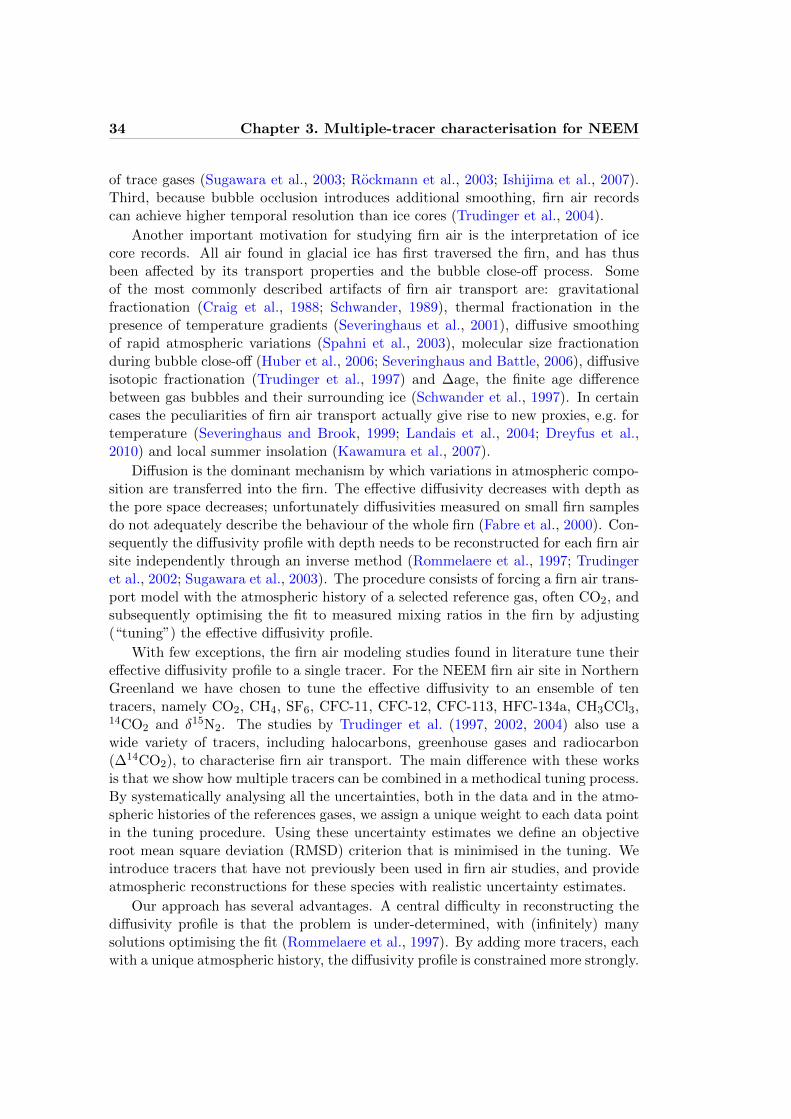
34 Chapter 3. Multiple-tracer characterisation for NEEM

of trace gases (Sugawara et al., 2003; Rockmann et al., 2003; Ishijima et al., 2007).Third, because bubble occlusion introduces additional smoothing, firn air recordscan achieve higher temporal resolution than ice cores (Trudinger et al., 2004).

Another important motivation for studying firn air is the interpretation of icecore records. All air found in glacial ice has first traversed the firn, and has thusbeen affected by its transport properties and the bubble close-off process. Someof the most commonly described artifacts of firn air transport are: gravitationalfractionation (Craig et al., 1988; Schwander, 1989), thermal fractionation in thepresence of temperature gradients (Severinghaus et al., 2001), diffusive smoothingof rapid atmospheric variations (Spahni et al., 2003), molecular size fractionationduring bubble close-off (Huber et al., 2006; Severinghaus and Battle, 2006), diffusiveisotopic fractionation (Trudinger et al., 1997) and ∆age, the finite age differencebetween gas bubbles and their surrounding ice (Schwander et al., 1997). In certaincases the peculiarities of firn air transport actually give rise to new proxies, e.g. fortemperature (Severinghaus and Brook, 1999; Landais et al., 2004; Dreyfus et al.,2010) and local summer insolation (Kawamura et al., 2007).

Diffusion is the dominant mechanism by which variations in atmospheric compo-sition are transferred into the firn. The effective diffusivity decreases with depth asthe pore space decreases; unfortunately diffusivities measured on small firn samplesdo not adequately describe the behaviour of the whole firn (Fabre et al., 2000). Con-sequently the diffusivity profile with depth needs to be reconstructed for each firn airsite independently through an inverse method (Rommelaere et al., 1997; Trudingeret al., 2002; Sugawara et al., 2003). The procedure consists of forcing a firn air trans-port model with the atmospheric history of a selected reference gas, often CO2, andsubsequently optimising the fit to measured mixing ratios in the firn by adjusting(“tuning”) the effective diffusivity profile.

With few exceptions, the firn air modeling studies found in literature tune theireffective diffusivity profile to a single tracer. For the NEEM firn air site in NorthernGreenland we have chosen to tune the effective diffusivity to an ensemble of tentracers, namely CO2, CH4, SF6, CFC-11, CFC-12, CFC-113, HFC-134a, CH3CCl3,14CO2 and δ15N2. The studies by Trudinger et al. (1997, 2002, 2004) also use awide variety of tracers, including halocarbons, greenhouse gases and radiocarbon(∆14CO2), to characterise firn air transport. The main difference with these worksis that we show how multiple tracers can be combined in a methodical tuning process.By systematically analysing all the uncertainties, both in the data and in the atmo-spheric histories of the references gases, we assign a unique weight to each data pointin the tuning procedure. Using these uncertainty estimates we define an objectiveroot mean square deviation (RMSD) criterion that is minimised in the tuning. Weintroduce tracers that have not previously been used in firn air studies, and provideatmospheric reconstructions for these species with realistic uncertainty estimates.

Our approach has several advantages. A central difficulty in reconstructing thediffusivity profile is that the problem is under-determined, with (infinitely) manysolutions optimising the fit (Rommelaere et al., 1997). By adding more tracers, eachwith a unique atmospheric history, the diffusivity profile is constrained more strongly.

3.2. Methods 35

The final reconstructed profile is a trade-off between the demands of the differenttracers. Second, many trace gases of interest, such as halocarbons, have a free airdiffusivity that differs from CO2 by up to a factor of 2. It is not a priori clear whethera profile tuned to CO2 alone provides a good solution for these gases. The tracers inthis study have a wide range of free air diffusivities, where the fastest tracer (CH4)has a free air diffusivity that is three times that of the slowest one (CFC-113). Third,when using ten tracers the available dataset is much larger, with several data pointsat each sampling depth. This makes the final result more robust, i.e. less susceptibleto effects of outliers and analytical biases. Finally, our method is less sensitive toerrors in the reconstructed atmospheric history of individual reference gases. Ouranalysis shows that uncertainties in the atmospheric reconstruction are the largestsource of potential error.

Apart from presenting a new methodology for characterising firn air sites, thiswork will also serve as a reference for other studies using NEEM firn air. Themodeling in a number of forthcoming publications in this issue will be based on thediffusivity reconstructions presented here.

We further present a model intercomparison between six state of the art one-dimensional firn air transport models. All the models are tuned to the same dataset,using the same physical firn parameters, such as porosity, free-air diffusion coeffi-cients, etc. To diagnose model performance we introduce four synthetic scenariosthat are designed to probe specific aspects of the model physics.

For many sections in this work more information is available in the Supplement.Because of the vast amount of material we have chosen to structure it the same as thiswork for easy referencing. Sections marked with an asterisk (∗) in this work have acorresponding section in the Supplement where additional information can be found.The Supplement also includes all the firn air data and atmospheric reconstructionsused in this study.

3.2 Methods

3.2.1 NEEM 2008 firn air campaign∗

The firn air used in this study was sampled during 14–30 July 2008 from two bore-holes near the NEEM deep ice core drilling site, Northern Greenland (77.45◦N51.06◦W). The sampling site was 1.5 km outside of the main camp and chosen toavoid contamination by going upwind of the prevailing wind direction. The two bore-holes, S2 and S3, were separated by 64 m. Firn air was sampled by drilling throughthe firn layers to the desired depth, and lowering the firn air sampling system intothe borehole. The sampling system consists of a purge and sample line, runningthrough an inflatable bladder to seal off the firn air from the overlying atmosphereduring sampling. S2 was sampled using the firn air system of the University of Bern(Schwander et al., 1993); S3 with the US firn air system (Battle et al., 1996). Forthis reason the boreholes are referred to as the “EU” and “US” holes, respectively.The CO2 mixing ratio was monitored on the purge line with LICOR (US site) and

36 Chapter 3. Multiple-tracer characterisation for NEEM

LIZDZ

CZ

0 10 20 30 40 50 60 70 80

0

0.1

0.2

0.3lock−

in depth

close−off depth

Depth (m)

0.4

0.5

0.6

0.7

0.8

0.9

0

2

4

6

8sop

scl

ρ (

g cm

−3 )

δ15N

2 (‰

)

porosity

×10−2

a

b

Figure 3.1: (a) Firn density ρ (left axis), and the open and closed porosity sop and scl, respectively(right axis). Black dots show firn density measurements in 0.55 m segments, the red line is the fitused in this study. (b) Gravitational enrichment as shown by δ15N2, corrected for thermal effects(Severinghaus et al., 2001). The blue line shows the barometric slope ∆Mg(z − 4.5)/RT , where weuse ∆M = 1 × 10−3 kg mol−1. Convective zone (CZ), diffusive zone (DZ) and lock-in zone (LIZ)are indicated by changes in shading.

MAIHAK (EU site) CO2 analysers to assess whether the firn air being pumped hadbeen purged of modern air prior to sampling. A site map and a complete list ofsampling depths can be found in the Supplement.

3.2.2 Physical characterisation of NEEM firn air site∗

We use the assumption commonly made in firn air modeling that the firn densityprofile is in steady state, and that the site has been climatically stable over thestudy period. For the firn density profile ρ(z) we use an empirical fit to the NEEMmain ice core density measurements averaged over 0.55 m segments (S. J. Johnsen,personal communication, 2009). For each of the three stages of the densificationprocess (Arnaud et al., 2000) we use a combination of quadratic and exponentialfunctions to fit the data, where care is taken that the derivative is continuous overthe transitions between the stages. The fit is generated on a ∆z = 0.2 m grid, whichis the spatial resolution used in this study. The density data and fit are shown inFig. 3.1a. Following the temperature relationship given by Schwander et al. (1997),a solid ice density ρice = 0.9206 g cm−3 is used.

3.2. Methods 37

We use an accumulation rate of A = 0.216 m yr−1 ice equivalent, as derived fromthe 2007 NEEM S1 shallow core (D. Dahl-Jensen, personal communication, 2010).Since the model runs cover the period 1800–2008 CE, we used the average rate overthe same period as a best estimate. This long-term average is slightly lower thanour best estimate for the current day accumulation of 0.227 m yr−1.

The total porosity s = 1 − ρ/ρice is divided into open and closed porosity (sop,scl) using the parameterisation of Goujon et al. (2003):

scl = 0.37s

(s

sco

)−7.6

(3.1)

where sco is the mean close-off porosity. The deepest point at which firn air could besampled successfully was z = 77.75 m. The depth of total pore closure (sop = 0) wasdetermined experimentally in the field by drilling the EU hole to a depth of z = 83 m,and subsequently raising the bladder in 0.5 m steps. The deepest point at which aircould be pulled was z = 79 m, though the flow was insufficient for sampling. To beconsistent with this observation we use sco = 9.708× 10−2 in Eq. (3.1), which leadsto total pore closure (sop = 0) at depth z = 78.8 m, as shown in Fig. 3.1a.

We use an annual mean site temperature of −28.9 ◦C as obtained from bore-hole thermometry on the EU hole, and assume an isothermal firn for this modelingexercise. Atmospheric pressure is 745 hPa.

Traditionally the firn column is divided into three zones, based on the gravita-tional enrichment with depth (Sowers et al., 1992). For NEEM the δ15N2 togetherwith the zonal division is shown in Fig. 3.1b. Using the barometric line fitting method(Kawamura et al., 2006), we obtain a convective zone (CZ) thickness of 4.5 m. Thezone below is called the diffusive zone (DZ), as diffusion dominates the transportat these depths. The lock-in depth is defined as the depth at which gravitationalenrichment stops, which happens at z = 63 m. Below we find the lock-in zone (LIZ),where advection with the ice matrix dominates the transport. This is also the regionwhere the majority of the bubble occlusion occurs, as can be seen from the scl curve.

3.2.3 Gas measurements∗

A total of 345 samples were taken from the boreholes, with atmospheric samplestaken at three occasions during the sampling period. Different flask types were used(SilcoCan, stainless steel flasks and glass flasks); for the tracers used in this studyno effect of flask type could be found in data comparison. We use firn air data fromsix different laboratories; an overview is given in Table 3.1.

Where applicable, data from IUP were corrected for known calibration offsets toplace all data on the NOAA scales used in the atmospheric reconstructions. After thecalibration correction no systematic offsets were observed between the different labo-ratories. As discussed below, there are significant offsets between the two boreholes,and data from the holes are not combined but treated separately. The ∆14CO2 dataand atmospheric reconstruction were both converted to a (mass conserving) ppmscale to allow 14CO2 to be modeled like a regular tracer. Wherever multiple data

38 Chapter 3. Multiple-tracer characterisation for NEEM

Table 3.1: Overview of firn air data used in this study. Acronyms represent: the School of En-vironmental Sciences at the University of East Anglia (UEA; Laube et al., 2010), NOAA EarthSystem Research Laboratory, Boulder CO (NOAA; Conway et al., 1994; Dlugokencky et al., 1994),the Institut fur Umweltphysik at the University of Heidelberg (IUP; Levin et al., 2010, 2011),the Commonwealth Scientific and Industrial Research Organisation, Marine and Atmospheric Re-search (CSIRO; Francey et al., 2003), the Australian Nuclear Science and Technology Organisation(ANSTO; Smith et al., 1999), and Scripps Institution of Oceanography at the University of Califor-nia, San Diego in collaboration with the National Institute of Polar Research, Japan (SIO/NIPR;Severinghaus et al., 2003).

Tracer EU borehole US borehole

CO2 NOAA, CSIRO, IUP NOAA, IUPCH4 NOAA, CSIRO NOAA, IUPSF6 NOAA, IUP, UEA NOAA, IUPCFC-11 UEA -CFC-12 UEA -CFC-113 UEA -HFC-134a UEA -CH3CCl3 UEA -∆14CO2 ANSTO -δ15N2 SIO/NIPR SIO/NIPRδ86Kr ∗ SIO/NIPR SIO/NIPR∗ Used for gravitational correction only

points were available for a certain depth, they were averaged in the following order:first replicate measurements from one laboratory were averaged, then the resultingvalues from the different labs were averaged. In this way one composite dataset wascreated that contains 204 data points for the 10 tracers on the EU hole, and 77 datapoints for the 4 tracers on the US hole. The δ15N2 profile is the same for both holes,and a combination of EU and US depths are used in the final dataset. This gives afinal dataset of 260 data points.

3.2.4 Reconstruction of atmospheric histories of selected tracers∗

A best-estimate atmospheric history was reconstructed for each of the referencetracers used in the tuning. Additionally we reconstructed a δ13CO2 history whichwas used to convert the ∆14CO2 reconstruction to a ppm scale (Stuiver and Polach,1977). Four different types of data were used in the reconstructions:

- Direct atmospheric measurements from sampling networks or archived air.Northern hemisphere high latitude stations (i.e. Alert, Summit and Barrow) are usedwhenever available. When using data from other stations a correction should be madeto account for the latitudinal gradient. This is done whenever the gradient could bereliably determined. We used station data from the NOAA-ESRL network for CO2,CH4, SF6 and HFC-134a (Conway et al., 1994; Dlugokencky et al., 1994; Geller et al.,1997; Montzka et al., 1996); from ALE/GAGE/AGAGE for CFC-11, CFC-12, CFC-113 and CH3CCl3 (Prinn et al., 2000, 2005; Cunnold et al., 1997; Fraser et al., 1996);from CSIRO for δ13CO2 (Francey et al., 2003). All ALE/GAGE/AGAGE data were

3.2. Methods 39

converted to NOAA calibrations scales; all δ13CO2 data are kept on the CSIRO cal-ibration scale. Furthermore we used the SIO Mauna Loa record for CO2 between1958–1985 CE (Keeling et al., 2009), and the Cape Grim air archive for δ13CO2

between 1978–1991 (Francey et al., 1999). The 14CO2 history between 1963–1993 isbased on Fruholmen, Norway, for its proximity to Greenland (Nydal and Lovseth,1996); data from other stations were used to complete time coverage (Manning andMelhuish, 1994; Levin and Kromer, 2004; Levin et al., 2008).

• High resolution firn air/ice core measurements from the high accumulation LawDome sites, Antarctica. The reconstructions of CO2 before 1958, and CH4

before 1983 are based on Etheridge et al. (1996, 1998) and MacFarling Meureet al. (2006); δ13CO2 before 1976 is based on Francey et al. (1999).

• Dendrochronologically-dated tree-ring measurements of radiocarbon. The re-construction of atmospheric 14CO2 before 1955 is based on Reimer et al. (2004).

• Emission-based estimates using a 2-D atmospheric transport model that in-cludes latitudinal source and sink distribution (Martinerie et al. (2009) andreferences therein). This has been used to complete time coverage for SF6 andhalocarbons before the onset of direct atmospheric measurements.

All the atmospheric reconstructions start in the year 1800 and have monthly resolu-tion. We use 2008.54 (mid July) as the decimal sampling date in the models. Whereapplicable the reconstructions were converted to the most recent NOAA scale to beconsistent with the data.

3.2.5 Gravitational correction∗

The gravitational fractionation of gases in the firn column with depth, δgrav(z), iswell established both theoretically and experimentally (Craig et al., 1988; Schwander,1989; Sowers et al., 1992). All data used in this study, with the exception of 15N2,have been corrected for the effect of gravity prior to the modeling. Consequentlythe models are run with either the molecular weight of all gases set equal to thatof air (M = Mair) or gravity set to zero (g = 0). Since the correction is based onactual measurements of δ86Kr (86Kr/82Kr), this procedure ensures that the effectof gravity is included correctly. When, on the other hand, the effect of gravity ishandled by the model, errors can be introduced when the modeled δgrav(z) deviatesfrom the true observed values. The empirical correction can potentially also be usedto correct for mass-dependent sampling artifacts (Severinghaus and Battle, 2006).

3.2.6 Differences between the EU and US boreholes

Though the boreholes are separated by a mere 64 m, within the lock-in zone we finddifferences in the mixing ratio profiles for CO2, CH4 (Fig. 3.2) and SF6 (not shown)that exceed the estimated uncertainty of the combined sampling-measurement pro-cedure (indicated with errorbar, see Sect. 3.2.7 for details). Note that we cannot

40 Chapter 3. Multiple-tracer characterisation for NEEM

330

340

350

360

370

EU boreholeUS borehole

LIZDZ62 64 66 68 70

1400

1500

1600

1700

1800

Depth (m)

CO

2 (pp

m)

CH

4 (pp

b)

a

b

Figure 3.2: Comparison of (a) CO2 and (b) CH4 data in the lock-in zone of the two boreholes.Data from three laboratories are averaged; the 1σ uncertainty bar is a combination of analyticaland sampling uncertainties as specified in Sect. 3.2.7. Curves are modeled profiles using the CICmodel, see Sect. 3.3.3.

make the same comparison for the other gas species since only data from the EUhole are available. We attribute these differences to lateral inhomogeneity in thefirn stratigraphy, possibly originating from surface wind features that have been pre-served in the densification process. Because of these differences we have chosen tomodel both holes separately.

For SF6 we furthermore observe a ∼ 0.25 ppt offset in the 5–50 m depth range,contrary to the CO2 and CH4 profiles that agree well between the holes at thesedepths. This excludes differences in age distribution of the air as the origin. Al-ternative explanations we considered, such as incomplete flask flushing, sample con-tamination, procedural blanks and bladder outgassing, could all be excluded. Sincewe found no objective reason to reject data from either hole, we account for thediscrepancy by assigning an additional errorbar to the SF6 data from both holes inthis depth range (see below).

3.3. Modeling firn air transport at NEEM 41

Table 3.2: Relative contributions to the total uncertainty, averaged over the firn column (EU bore-hole).

Tracer Analytical Reconstruction Contamination Sampling Other

CO2 0.02 0.47 0.00 0.17 0.15a, 0.19b

CH4 0.08 0.85 0.01 0.05 -SF6 0.07 0.54 0.04 0.08 0.27c

CFC-11 0.11 0.81 0.04 0.04 -CFC-12 0.35 0.48 0.06 0.11 -CFC-113 0.55 0.38 0.04 0.03 -HFC-134a 0.29 0.63 0.04 0.04 -CH3CCl3 0.10 0.73 0.00 0.17 -∆14CO2 0.14 0.80 0.00 0.00 0.06a

δ15N2 0.91 - 0.05 0.04 -a In situ artifactsb Undersampling of seasonal cyclec EU-US borehole SF6 offset

3.2.7 Full uncertainty estimation∗

Having accurate uncertainty estimates is essential for our multiple-tracer methodol-ogy. A unique uncertainty estimate has been assigned to each of the 260 individualdata points used in this study based on the following seven potential sources of un-certainty: (1) analytical precision as specified by the laboratories. (2) Uncertaintyin atmospheric reconstructions. (3) Contamination with modern air in the deepestfirn samples; the estimates are based on HFC-134a, SF6 and CFCs, which should beabsent in the deepest samples. (4) Sampling effects estimated from inter-laboratoryand inter-borehole offsets. (5) Possibility of in-situ CO2 artifacts (e.g. Tschumi andStauffer, 2000) and CO2 enrichment due to close-off fractionation (Huber et al., 2006;Severinghaus and Battle, 2006). (6) Undersampling of seasonal cycle in the monthlyatmospheric reconstruction (CO2 only). (7) Large unexplained EU-US borehole dif-ference in the diffusive zone (SF6 only).

The errors are assumed to be independent of each other. The uncertainties inthe atmospheric reconstructions are converted from a time scale to a depth scale byrunning them through the CIC firn air model (Sect. 3.3.2). Details are given in theSupplement. The relative contribution of the seven sources, averaged over the firncolumn, is given in Table 3.2. For most tracers the atmospheric reconstruction is thelargest contributor to the total uncertainty, followed by the analytical precision.

3.3 Modeling firn air transport at NEEM

3.3.1 Tuning of the diffusivity profile∗

How the diffusive transport changes with depth needs to be reconstructed throughan inverse method for each firn air site independently. The procedure consists offorcing the transport models with the atmospheric history of one or several selected

42 Chapter 3. Multiple-tracer characterisation for NEEM

reference tracer(s), and subsequently optimising the fit to the measured mixing ratiosin the firn by adjusting the effective diffusivity values at each depth (Rommelaereet al., 1997; Trudinger et al., 2002; Sugawara et al., 2003).

Here we will use diffusion as a generic term for mass transfer processes that aredriven by a concentration gradient, and well described by Fick’s law. The diffusivityprofile we reconstruct is composed of two parts:

Molecular diffusion is a microscopic process originating in the thermal motion ofthe molecules constituting the firn air. The effective molecular diffusion coefficientof gases in the open porosity decreases with depth as the diffusive path becomesincreasingly tortuous due to the densification process (Schwander et al., 1988). Thediffusion coefficient of gas X at depth z is given by

DX(z) = sopD0X

τ(z)= sopγX

D0CO2

τ(z)(3.2)

where D0X is the diffusion coefficient in free air, τ(z) is the tortuosity at depth z,

and γX = DX/DCO2 is the ratio of diffusion coefficients (Trudinger et al., 1997).It is clear from Eq. (3.2) that the molecular diffusivity profiles for the different gasspecies scale linearly with each other. The γX used in this study are based onmeasurements by Matsunaga et al. (1993, 1998, 2002a,b), or a theoretical formula(Chen and Othmer, 1962) for gas species where no experimental data are available(Supplement).

Eddy diffusion refers to mass transfer caused by air flow patterns in the open porositywhich the models cannot resolve directly, and are instead parameterised through theinclusion of a diffusion coefficient Deddy(z). Unlike molecular diffusion, Deddy isequal for all gases as the process is macroscopic in origin. The first contributionto Deddy is convective mixing in the top few meters due to seasonal temperaturegradients and wind pumping (Colbeck, 1989; Severinghaus et al., 2001; Kawamuraet al., 2006). Some of the models also include a Deddy term in the deep firn torepresent dispersive mass transfer. The classical example of dispersive mixing isTaylor dispersion, where (viscous) shear flow in a circular tube enhances the effectivediffusivity of a solute (Aris, 1956). Viscous flow can be induced in the deep firn bylow frequency pressure fluctuations at the surface (Schwander, 1989), as well as airexpulsion due to pore compaction (Rommelaere et al., 1997). In soils, viscous flowinduced by atmospheric pressure fluctuations has been shown to be an importanttransport mechanism (Massmann and Farrier, 1992). Pore compaction causes a non-uniform velocity distribution between air expelled upwards, and air remaining behindin the pores. This spread in velocities results in additional (dispersive) mixing.

The extensive uncertainty analysis we introduced in Sect. 3.2.7 assesses how re-liable each data point is, and consequently how much weight should be assignedto it in the tuning procedure. This allows us to combine multiple tracers in thetuning, and the final reconstructed diffusivity profile is a trade-off between the con-straints placed by the different tracers. All models in this study tuned their effective

3.3. Modeling firn air transport at NEEM 43

Table 3.3: Overview of firn air transport models. See text for explanation.

Model Coordinates Advection Convection Time stepping Tuning

CIC static flux exponential Crank-Nic. automatedCSIRO moving coordinates exponential Crank-Nic. automatedINSTAAR static flux exponential explicit manualLGGE-GIPSA static flux tuned implicit automatedOSU static boxes exponential Crank-Nic. manualSIO static boxes exponential explicit automated

diffusivity profiles to minimise the root mean square deviation

RMSD =

(1

N

N∑i=1

(mi − di)2

σ2i

) 12

(3.3)

where the di are the data for a given borehole (all tracers), mi are the linearlyinterpolated modeled values at the same depths, and σi give the total uncertainties.The index i runs over all data points, where N = 204 for the EU hole, and N = 77for the US hole.

3.3.2 Model description∗

Six 1-D firn air transport models are tuned to the NEEM 2008 firn air data in theway outlined above. The models (in alphabetical order) were developed at the Cen-tre for Ice and Climate (CIC), Commonwealth Scientific and Industrial ResearchOrganisation (CSIRO, Trudinger et al., 1997), Institute of Arctic and Alpine Re-search (INSTAAR), Laboratoire de Glaciologie et Geophysique de l’Environnementand Grenoble Image Parole Signal Automatique (LGGE-GIPSA, Witrant et al.,2011), Oregon State University (OSU) and the Scripps Institution of Oceanography(SIO, Severinghaus and Battle, 2006).

Table 3.3 summarises a selection of relevant model characteristics. The secondcolumn indicates the kind of coordinate system used by each model. The CSIROmodel is unique in using a coordinate system that moves downwards with descendingice layers (Lagrangian coordinates), giving a downward ice velocity wice = 0 relativeto the reference frame. The other models use a static (Eulerian) coordinate systemwhere the surface stays at z = 0 and the ice layers move down at a finite velocitywice = Aρ/ρice. The choice of coordinate system has consequences for the way ad-vection of air with the ice matrix is handled (third column). In the CSIRO modelthe moving coordinate system automatically leads to advective transport withoutthe need to include it explicitly. The models expressed in Eulerian coordinates useeither an advective flux as described by Rommelaere et al. (1997), or use boxes ofair that are shifted downwards at regular time intervals (Schwander et al., 1993).Convection (fourth column) is handled in two different ways. The LGGE-GIPSAmodel uses a Deddy term that is tuned by the RMSD minimisation algorithm, incombination with zero gravitational fractionation for z < 4 m. The other models use

44 Chapter 3. Multiple-tracer characterisation for NEEM

the parameterisation of Kawamura et al. (2006) where a Deddy term is included thatfalls off exponentially with depth. The fifth column of Table 3.3 indicates whetherthe time stepping used in solving the diffusion equation was either explicit (Eu-ler forward), implicit (Euler backward) or mixed implicit-explicit (Crank-Nicolsonmethod). Finally, some of the models were tuned through manual adjustments of thediffusivity profile, while others used an automated control method (e.g. Rommelaereet al., 1997; Trudinger et al., 2002).

3.3.3 Fit of modeled profiles to the data∗

The modeled profiles for all 10 tracers from the EU borehole are shown in Fig. 3.3,profiles from the US borehole can be found in the Supplement.

For CO2 (Fig. 3.3a) we find a pronounced mismatch for z > 70 m which is re-produced consistently by all models and in both boreholes. The atmospheric recon-struction is based on the Law Dome record (Etheridge et al., 1996), and consequentlythe largest source of uncertainty is the interhemispheric CO2 gradient. To explainthe observed mismatch with an error in the atmospheric history would require a6 ppm interhemispheric gradient in the 1950s, which can be ruled out (Keeling et al.,2010). Also contamination with modern air can be ruled out for these flasks, basedon measurements of halocarbons. We cannot, however, exclude in-situ productionof CO2 from e.g. organic material or (bi)carbonates found in Greenland ice (e.g.Tschumi and Stauffer, 2000). There might also be a small close-off fractionation ofCO2, of order 1 h or less, based on its effective molecular diameter (Huber et al.,2006; Severinghaus and Battle, 2006).

Both CH3CCl3 and 14CO2 (Fig. 3.3d–e) have a peak within the LIZ. The peakheight and position, which are sensitive to the shape and magnitude of the diffusivityprofile, provide an important constraint in the tuning procedure. It is exactly atthese peaks that the divergence between the models is most easily visible. It mustbe noted, however, that equally large model differences are found for other tracers aswell (e.g. CO2 and HFC-134a). Furthermore, models that fit the peak height exactlydo not necessarily provide the best overall fit to the data.

To quantitatively assess how well the modeled profiles fit the data, we make ahistogram of (mi − di)/σi where the index i goes over all 204 data points of the EUborehole. The σi are the unique uncertainties we assigned to each data point. This isshown in Fig. 3.4 together with a Gaussian distribution of width σ = 1 and a surfacearea equal to that of the histogram. The figure furthermore shows the RMSD fromthe data as given by Eq. (3.3). For all models we find a distribution that is morenarrow than the Gaussian distribution, meaning that within the assigned uncertain-ties all data from the borehole can be modeled consistently. The good agreementgives confidence in the correctness of our reconstructed atmospheric histories, whichwill be of use in future firn air studies. For the US hole the RMSD ranges between0.60–1.06.

Two models stand out as having a larger RMSD of 0.92 (CSIRO and OSU).For the CSIRO model this is caused by the absence of a back flow due to pore

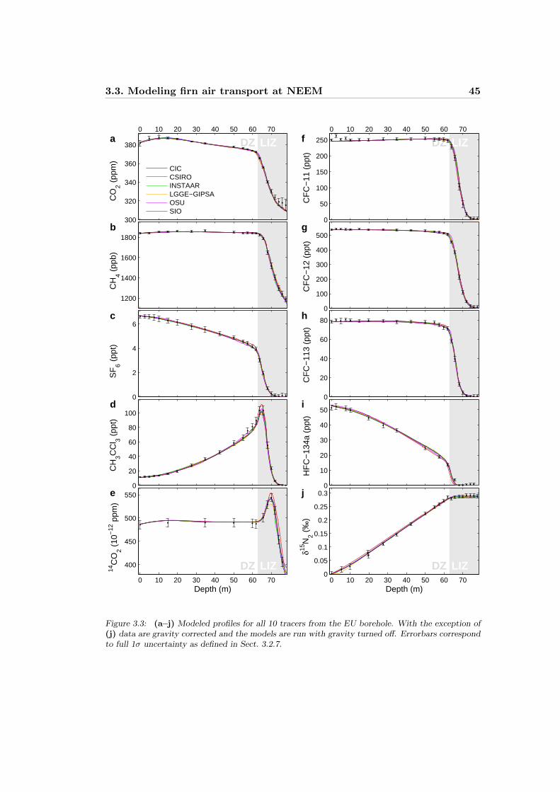
3.3. Modeling firn air transport at NEEM 45

LIZDZ0 10 20 30 40 50 60 70

300

320

340

360

380

CICCSIROINSTAARLGGE−GIPSAOSUSIO

1200

1400

1600

1800

0

2

4

6

0

20

40

60

80

100

LIZDZ0 10 20 30 40 50 60 70

400

450

500

550

Depth (m)

LIZDZ0 10 20 30 40 50 60 70

0

50

100

150

200

250

0

100

200

300

400

500

0

20

40

60

80

0

10

20

30

40

50

LIZDZ0 10 20 30 40 50 60 70

0

0.05

0.1

0.15

0.2

0.25

0.3

Depth (m)

CO

2 (pp

m)

CH

4 (pp

b)S

F6 (

ppt)

CH

3CC

l 3 (pp

t)14

CO

2 (10

−12

ppm

)

CF

C−

11 (

ppt)

CF

C−

12 (

ppt)

CF

C−

113

(ppt

)H

FC

−13

4a (

ppt)

δ15N

2 (‰

)

a

b

c

d

e

f

g

h

i

j

Figure 3.3: (a–j) Modeled profiles for all 10 tracers from the EU borehole. With the exception of(j) data are gravity corrected and the models are run with gravity turned off. Errorbars correspondto full 1σ uncertainty as defined in Sect. 3.2.7.

46 Chapter 3. Multiple-tracer characterisation for NEEM

−4 −2 0 2 4

0

10

20

30 CIC RMSD= 0.73

Cou

nts

−4 −2 0 2 4

0

10

20

30 CSIRO RMSD= 0.92

Cou

nts

0

10

20

30 INSTAAR RMSD= 0.78

Cou

nts

0

10

20

30 LGGE−GIPSARMSD= 0.74

Cou

nts

−4 −2 0 2 40

10

20

30 OSU RMSD= 0.92

(Model−data) / σ

Cou

nts

−4 −2 0 2 40

10

20

30 SIO RMSD= 0.80

(Model−data) / σ

Cou

nts

a b

c d

e f

Figure 3.4: (a–f) Histogram of (mi − di)/σi for the firn air transport models in this study usingthe EU borehole data. The black curve gives a Gaussian distribution of width σ = 1, normalised tohave equal surface to the histogram. The RMSD is calculated using Eq. (3.3).

compression in the transport description (Sect. 3.4.4.4). For the OSU model weattribute the larger RMSD to the tuning procedure for the molecular diffusivity,which has fewer degrees of freedom than the procedures used by the other models(Supplement).

Differences in RMSD give information on the performance of models, or modelconfigurations, relative to each other; the RMSD as defined by Eq. (3.3) should notbe interpreted in an absolute sense.

3.4 Model intercomparison and discussion

3.4.1 Diffusivity profiles∗

All the models are tuned separately to optimise the fit to the data. Figure 3.5ashows the reconstructed molecular diffusivity profiles for CO2. The spread betweenthe solutions is caused by two factors. First, it reflects differences in model physics,

3.4. Model intercomparison and discussion 47

LIZDZ0 10 20 30 40 50 60 70

0

0.5

1

1.5

10−9

10−8

10−7

10−6

10−5

CICCSIROINSTAARLGGE−GIPSAOSUSIO

0 10 20 30 40 50 60 70

0

0.2

0.4

0.6

0.8

1

Depth (m)

a

b

c

DC

O2 (

10−

5 m2 /s

)D

tota

l (m

2 /s)

Ded

dy /

Dto

tal

Figure 3.5: (a) CO2 molecular diffusivity profile with depth DCO2(z) for the EU borehole. (b)Semi-log plot of the total CO2 diffusivity profile Dtotal(z) = DCO2(z) + Deddy. (c) Plot ofDeddy(z)/Dtotal(z). Eddy diffusion near the surface corresponds to convective mixing; in the LIZsome of the models include dispersive mixing. The CSIRO model has zero eddy diffusivity in theLIZ; the line is not visible as the LGGE-GIPSA model is plotted on top of it.

which are compensated for by adjustments to the diffusivity profile. Second, it relatesto the degree in which the inverse problem of diffusivity reconstruction is under-determined. By using 10 different tracers the problem is more strongly constrainedthan in the case of using only CO2, but the solution is not unique.

A second important observation is that all models require a non-vanishing diffu-sivity on the order of 2×10−9m2s−1 within the LIZ (see Fig. 3.5b). This contradictsthe notion that diffusivity vanishes completely in the LIZ due to the presence of im-permeable layers, which is frequently expressed in firn air studies (e.g. Battle et al.,1996; Trudinger et al., 2002; Assonov et al., 2005). Our findings confirm a recentstudy at Megadunes, Antarctica, that also reports a finite (eddy) diffusivity in the

48 Chapter 3. Multiple-tracer characterisation for NEEM

LIZ (Severinghaus et al., 2010). We believe this result to be robust, since it is re-produced by all six firn air models. In particular, the well reproduced height of the14CO2 bomb spike, which falls entirely within the LIZ, provides strong evidence forfinite LIZ diffusion at NEEM; letting diffusivity go to zero leads to a 14CO2 peakthat is too narrow and overshoots the measured values by ∼ 7σ.

How the LIZ diffusivity is parameterised, however, varies strongly among themodels as shown in Fig. 3.5c. The models use either molecular diffusion, dispersivemixing (eddy diffusion) or a mixture of both. To fit the δ15N2 data, most modelsrequire some dispersive mixing in the LIZ, since molecular diffusion alone would leadto continued gravitational fractionation. The LGGE-GIPSA model circumvents thisproblem by using a combination of Fick’s and Darcy’s transport to describe almost-stagnant transport in the lower zones (Witrant et al., 2011), which allows for usingpurely molecular diffusion in the LIZ. The SIO model uses the ratio of eddy to molec-ular diffusion in the LIZ as a tuning parameter in the RMSD minimisation, and findsthat the fit is optimised for 27 % eddy diffusion (Supplement). Models that repro-duce the observations equally well can have completely different parameterisations,so our analysis does not tell us which scheme is more likely to be correct. Thesemodel differences do have important consequences for the modeling of isotopic ratios,as is discussed below.

3.4.2 Gas age distributions∗

Firn air does not have a single age, but rather a distribution of ages (Schwanderet al., 1993). The modeled gas age distribution, also referred to as Green’s function,transfer function, response function or age spectrum, provides a complete descriptionof the model transport properties (Rommelaere et al., 1997). Figure 3.6 comparesCO2 age distribution densities for the models at the lock-in depth (z = 63 m) andat the bottom of the LIZ (z = 78 m, close to the deepest EU hole sample at z =77.75 m). The most relevant characteristics of the age distributions are summarisedin Table 3.4. As a measure of the relative spread in model results, we list the 2σstandard deviation divided by the mean (µ).

The LIZ lies between the two depths depicted here. From the closed porosityparameterisation (Eq. 3.1), we find that ∼ 95 % of the air is trapped in this zone. Thegas age distribution found in NEEM ice below the full close-off depth (sop = 0) willbe intermediate to these two end members, with a tail of older air trapped alreadyin the DZ. Interestingly, at the lock-in depth (z = 63 m), estimates of both theage and the distribution width show a spread of around 25 % between models thatreproduce the data equally well. Clearly these properties are not as well determinedas one would expect based on the similarity between the modeled curves alone. Ontraversing the LIZ to z = 78 m the relative spread in modeled ages is reduced; theabsolute spread grows slightly to about 5 yr, though. The spread in distributionwidths remains large.

For the US borehole the spread in the calculated mean ages at z = 63 m is evenup to 40 %. This larger spread is due to the fact that we have only 4 tracers on the

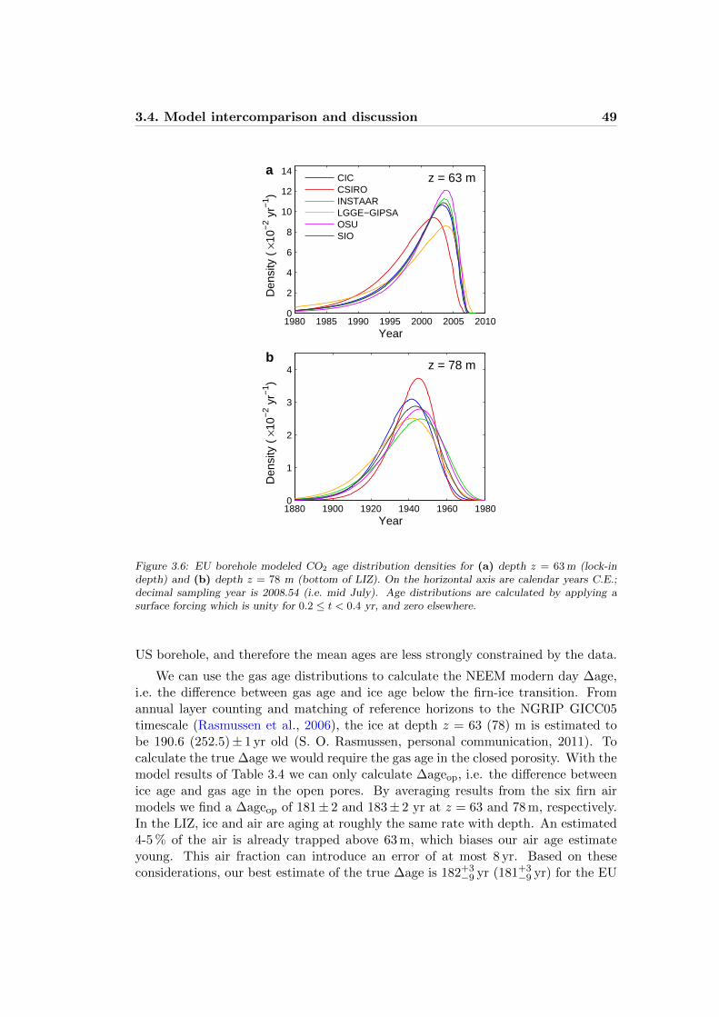
3.4. Model intercomparison and discussion 49

1980 1985 1990 1995 2000 2005 20100

2

4

6

8

10

12

14

Year

z = 63 mCIC

CSIROINSTAARLGGE−GIPSAOSUSIO

1880 1900 1920 1940 1960 19800

1

2

3

4

Year

z = 78 m

Den

sity

( ×

10−

2 yr−

1 )D

ensi

ty (

×10

−2 y

r−1 )

a

b

Figure 3.6: EU borehole modeled CO2 age distribution densities for (a) depth z = 63 m (lock-indepth) and (b) depth z = 78 m (bottom of LIZ). On the horizontal axis are calendar years C.E.;decimal sampling year is 2008.54 (i.e. mid July). Age distributions are calculated by applying asurface forcing which is unity for 0.2 ≤ t < 0.4 yr, and zero elsewhere.

US borehole, and therefore the mean ages are less strongly constrained by the data.

We can use the gas age distributions to calculate the NEEM modern day ∆age,i.e. the difference between gas age and ice age below the firn-ice transition. Fromannual layer counting and matching of reference horizons to the NGRIP GICC05timescale (Rasmussen et al., 2006), the ice at depth z = 63 (78) m is estimated tobe 190.6 (252.5)± 1 yr old (S. O. Rasmussen, personal communication, 2011). Tocalculate the true ∆age we would require the gas age in the closed porosity. With themodel results of Table 3.4 we can only calculate ∆ageop, i.e. the difference betweenice age and gas age in the open pores. By averaging results from the six firn airmodels we find a ∆ageop of 181± 2 and 183± 2 yr at z = 63 and 78 m, respectively.In the LIZ, ice and air are aging at roughly the same rate with depth. An estimated4-5 % of the air is already trapped above 63 m, which biases our air age estimateyoung. This air fraction can introduce an error of at most 8 yr. Based on theseconsiderations, our best estimate of the true ∆age is 182+3

−9 yr (181+3−9 yr) for the EU

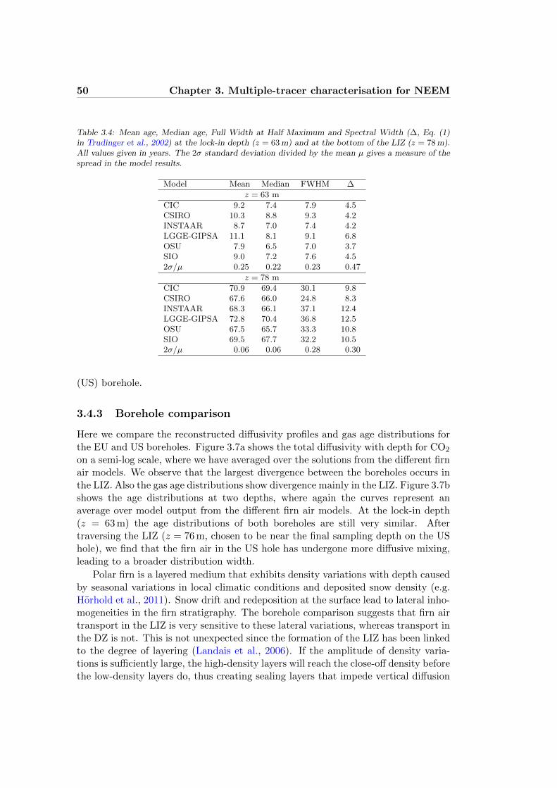
50 Chapter 3. Multiple-tracer characterisation for NEEM

Table 3.4: Mean age, Median age, Full Width at Half Maximum and Spectral Width (∆, Eq. (1)in Trudinger et al., 2002) at the lock-in depth (z = 63 m) and at the bottom of the LIZ (z = 78 m).All values given in years. The 2σ standard deviation divided by the mean µ gives a measure of thespread in the model results.

Model Mean Median FWHM ∆

z = 63 m

CIC 9.2 7.4 7.9 4.5CSIRO 10.3 8.8 9.3 4.2INSTAAR 8.7 7.0 7.4 4.2LGGE-GIPSA 11.1 8.1 9.1 6.8OSU 7.9 6.5 7.0 3.7SIO 9.0 7.2 7.6 4.52σ/µ 0.25 0.22 0.23 0.47

z = 78 m

CIC 70.9 69.4 30.1 9.8CSIRO 67.6 66.0 24.8 8.3INSTAAR 68.3 66.1 37.1 12.4LGGE-GIPSA 72.8 70.4 36.8 12.5OSU 67.5 65.7 33.3 10.8SIO 69.5 67.7 32.2 10.52σ/µ 0.06 0.06 0.28 0.30

(US) borehole.

3.4.3 Borehole comparison

Here we compare the reconstructed diffusivity profiles and gas age distributions forthe EU and US boreholes. Figure 3.7a shows the total diffusivity with depth for CO2

on a semi-log scale, where we have averaged over the solutions from the different firnair models. We observe that the largest divergence between the boreholes occurs inthe LIZ. Also the gas age distributions show divergence mainly in the LIZ. Figure 3.7bshows the age distributions at two depths, where again the curves represent anaverage over model output from the different firn air models. At the lock-in depth(z = 63 m) the age distributions of both boreholes are still very similar. Aftertraversing the LIZ (z = 76 m, chosen to be near the final sampling depth on the UShole), we find that the firn air in the US hole has undergone more diffusive mixing,leading to a broader distribution width.

Polar firn is a layered medium that exhibits density variations with depth causedby seasonal variations in local climatic conditions and deposited snow density (e.g.Horhold et al., 2011). Snow drift and redeposition at the surface lead to lateral inho-mogeneities in the firn stratigraphy. The borehole comparison suggests that firn airtransport in the LIZ is very sensitive to these lateral variations, whereas transport inthe DZ is not. This is not unexpected since the formation of the LIZ has been linkedto the degree of layering (Landais et al., 2006). If the amplitude of density varia-tions is sufficiently large, the high-density layers will reach the close-off density beforethe low-density layers do, thus creating sealing layers that impede vertical diffusion

3.4. Model intercomparison and discussion 51

LIZDZ

0 10 20 30 40 50 60 7010

−9

10−8

10−7

10−6

10−5

Depth (m)

EU boreholeUS borehole

1900 1920 1940 1960 1980 20000

2

4

6

8

10

12

z = 63 m

z = 76 m

Year

a

b

Dto

tal (

m2 /s

)D

ensi

ty (

×10

−2 y

r−1 )

Figure 3.7: Comparison between the EU and US boreholes. (a) Semi-log plot of the total CO2 dif-fusivity profile Dtotal(z) = DCO2(z) +Deddy averaged over all six firn models. (b) Age distributionsat depths z = 63 m (lock-in depth) and z = 76 m (bottom of LIZ) averaged over five firn models.The CSIRO model is excluded in the age distribution comparison as the US age distribution atz = 76 m is unreliable (Supplement).

and prevent further gravitational fractionation of the gas mixture (Martinerie et al.,1992; Schwander et al., 1993; Sturrock et al., 2002). Earlier we presented evidencefor finite vertical mixing in the LIZ despite the presence of such impeding layers.The amount of vertical mixing is expected to depend on the horizontal extent of thesealing layers, as well as the position of (micro)cracks and passageways. This couldlead to a strong lateral variation in LIZ diffusion as observed. Note that such lateralprocesses cannot be represented adequately in one-dimensional transport models.

3.4.4 Synthetic diagnostic scenarios∗

To diagnose model properties further, we developed four synthetic scenarios thatprobe specific aspects of the model physics. We present the individual scenariosbelow, and discuss the model differences they reveal.

52 Chapter 3. Multiple-tracer characterisation for NEEM

0 10 20 30 40 50 60 70

−0.14

−0.12

−0.1

−0.08

−0.06

−0.04

−0.02

0

CICCSIROINSTAARLGGE−GIPSAOSUSIO

0 10 20 30 40 50 60 70

10−4

10−3

10−2

10−1

100

LIZDZ0 10 20 30 40 50 60 70

0

0.05

0.1

0.15

0.2

0.25

0.3

Depth (m)

LIZDZ0 10 20 30 40 50 60 70

0

200

400

600

800

Depth (m)

δ13C

O2 (

‰)

δ grav

(‰

)

Am

plitu

de |c

|A

ge o

f air

(yrs

)

a b

c d

Figure 3.8: Model comparison using the four diagnostic scenarios and diffusivity tuned to the EUborehole data. (a) Scenario I: diffusive fractionation for a hypothetical monotonic CO2 increase.(b) Scenario II: attenuation of a 15 yr period sinusoidal CO2 forcing with depth. (c) Scenario III:gravitational enrichment for gas X with D0

X = 0.025D0CO2

. Data show gravitational enrichmentof 15N2 corrected for the effect of thermal diffusion. See Supplement for details. (d) Scenario IV:mean age of gas Y when using advective transport only (D0

Y = 0, i.e. diffusion is absent). With theexception of S-III all scenarios were run with the effect of gravity turned off.

3.4.4.1 Scenario I: diffusive fractionation

For gas species whose atmospheric mixing ratios change over time, the disequilibriumin the firn leads to an isotopic fractionation with depth, even in the absence ofchanges in atmospheric isotopic composition (Trudinger et al., 1997). As a scenariowe use a monotonic CO2 increase of ∼1 ppm yr−1 without seasonal cycle, chosento resemble the current anthropogenic increase (Keeling et al., 2010). The surfaceisotopic ratio is kept fixed at δ13CO2 = 0. Because the 13CO2 isotopologue has alower diffusivity, it is transported less efficiently into the firn, leading to a depletionin 13CO2 with depth. Ice core and firn air records need to be corrected for the effectof diffusive fractionation (DF). For example, the (site specific) corrections for therecent anthropogenic increase are ∼0.1 h for δ13CO2 at DE08, Law Dome (Franceyet al., 1999), and 1.2 h for δ13CH4 at WAIS-Divide (Mischler et al., 2009).

Figure 3.8a shows the modeled isotopic signal with depth for the different mod-els. Results in the DZ are consistent, however they diverge strongly once the LIZ

3.4. Model intercomparison and discussion 53

is reached. For δ13C of CO2, the observed range between the different model so-lutions in the deepest firn is 0.05 h, which is around 40 % of the total DF signal.For isotopologues of CH4 the DF is larger, because of the larger relative mass dif-ference between the isotopologues. Based on the observed DF model disagreementwe estimate an uncertainty of 0.5 h for both δ13C and δD of CH4. For δD of CH4

this uncertainty is smaller than the typical measurement uncertainty, as well as theatmospheric signal observed in the firn (Braunlich et al., 2001; Mischler et al., 2009).However, for both δ13CO2 and δ13CH4 the model disagreement exceeds the typicalinstrumental precision. At this moment we have no objective way of determiningwhich of the models predicts the DF correctly. This additional uncertainty shouldtherefore be recognised when interpreting ice core and firn gas isotopic records ofperiods with rapid atmospheric variations. Sites with a thick LIZ, combined witha low accumulation rate, allow for reconstructing atmospheric mixing ratios furtherback in time. However, a thick LIZ also means a larger uncertainty in DF (andthereby isotopic reconstruction) due to the poorly constrained LIZ transport.

Molecular diffusion leads to DF between isotopologues because their diffusioncoefficients are different. Advection, convection and dispersive mass transfer donot discriminate between isotopologues, and consequently do not fractionate thegas mixture. The observed model disagreement originates in the way in which LIZtransport is parameterised (Fig. 3.5c). The CIC and OSU models both smoothly gofrom purely molecular diffusion in the DZ to purely eddy diffusion in the LIZ. Oncethe molecular diffusion reaches zero, the DF ceases to increase with depth giving ahorizontal line. The LGGE-GIPSA model on the other hand uses molecular diffusionall the way down to the close-off depth, giving a continued fractionation with depth.One way the DF uncertainty could be incorporated in future studies is by testingdifferent parameterisations for LIZ diffusion, or by using transfer functions generatedby different models.

The Law Dome-based records of δ13CO2 (Francey et al., 1999) and δ13CH4 (Fer-retti et al., 2005) were both corrected for the effects of DF. The correction shouldnot be affected much by our findings here for several reasons. Most importantly, theaccumulation rate (and therefore the advective flux) at the Law Dome DE08 andDE08-2 sites is very large. This will strongly reduce DF in the LIZ as describedabove. Furthermore the LIZ is relatively thin (Trudinger, 2001). The study byFerretti et al. (2005) combines ice core samples from the aforementioned high accu-mulation Law Dome sites with firn air measurements from the DSSW20K site, whichhas a rather low accumulation rate (∼ 0.16 m yr−1 ice equivalent). After DF correc-tion the results agree well. In other published firn air and ice core isotopic recordsthat cover the recent anthropogenic increase (e.g. Braunlich et al., 2001; Sugawaraet al., 2003; Rockmann et al., 2003; Sowers et al., 2005; Bernard et al., 2006; Ishijimaet al., 2007; Mischler et al., 2009) the uncertainty in the reconstruction due to theDF correction might have been underestimated.

54 Chapter 3. Multiple-tracer characterisation for NEEM

3.4.4.2 Scenario II: attenuation of a sine wave with depth

Rapid atmospheric variations are attenuated in the firn, and recorded in the ice witha reduced amplitude (Spahni et al., 2003). To compare the firn smoothing effectbetween the models, we force them with a sinusoidal atmospheric variation in CO2

that has a 15 yr period. Due to diffusion, the amplitude of the signal decreases withdepth in the firn. For mathematical convenience we impose two separate atmosphericscenarios:

[C1](t, z = 0) = 1 + sin (2πt/15)

[C2](t, z = 0) = 1 + cos (2πt/15)

where t is the time in years. Note that both signals are attenuated to the samedegree, and that the π/2 phase angle between them is preserved. To get the signalamplitude with depth, we combine them in the following way:

|[C](t, z)| =√

([C1](t, z)− 1)2 + ([C2](t, z)− 1)2 (3.4)

The outcome is shown in Fig. 3.8b. We observe that signal attenuation in theLIZ is stronger than in the DZ. This is because transport in the DZ is efficient; themean CO2 age at the lock-in depth is around 9 yr, which is less than the period ofthe atmospheric oscillation. The mixing ratios in most of the DZ will be “in phase”with the atmospheric signal, giving little attenuation. By comparison, air in the LIZis nearly stagnant. It takes around 70 yr to be transported over 15 m, correspondingto almost 5 periods of the sinusoid. As air of different ages (i.e. different phases ofthe atmospheric cycle) gets mixed, the signal amplitude is reduced.

Within the DZ the models agree well. In the LIZ there are two intervals (65 < z <68 m and 74 < z < 78 m) where the CSIRO model has significantly less attenuationwith depth. These intervals correspond to the depths where the reconstructed CSIROdiffusivity goes to zero (Fig. 3.5b). On the US borehole this effect is even morepronounced (Supplement).

Earlier we touched upon the question of whether or not there is continued dif-fusion in the LIZ; our diffusivity reconstructions indicate that there is at NEEM.Scenario II shows that this remnant LIZ diffusivity causes very strong attenuationof the atmospheric signal. Therefore, the question of LIZ diffusivity has impor-tant consequences for the temporal resolution at which we can hope to reconstructatmospheric variations back in time using ice cores.

3.4.4.3 Scenario III: balance of transport fluxes

The total gas flux is the sum of the advective, diffusive and convective fluxes. Withinthe DZ, molecular diffusion overwhelms the other transport mechanisms; in thisscenario we bring the different fluxes into balance by considering a hypotheticalgas X with a very small diffusion coefficient D0

X = 0.025D0CO2

, and a mass MX =

3.4. Model intercomparison and discussion 55

Mair +1×10−3 kg mol−1. The relative strength of the different mechanisms is shownby the gravitational enrichment with depth.

Figure 3.8c shows the model output together with the true gravitational enrich-ment as measured for 15N2. In thermodynamic equilibrium the enrichment is givenby the barometric equation: δgrav(z) = [exp(∆Mgz/RT )− 1] ≈ ∆Mgz/RT (Sowerset al., 1992). The advective and convective fluxes drive the air column out of equi-librium reducing δgrav(z) below the barometric case. For gas X the diffusive flux isnot large enough to oppose the other two, leading to a final δgrav which is about halfthat of 15N2. In this way the enrichment with depth represents the balance betweendiffusion on one hand, and advection and convection on the other.

The differences in implementation of the convective mixing are clearly visible.The LGGE-GIPSA model uses no gravitational enrichment in the top 4 m, followedby a tuned eddy diffusion. The convective mixing in the other models, which all usethe parameterisation by Kawamura et al. (2006), penetrates much deeper into thefirn. In the DZ there are also clear differences; here the gravitational slope mostlyrepresents the balance between diffusion and advection. The CSIRO has a strongeradvection term due to the absence of pore compression back flow (see below); this isreflected in a more reduced slope. A higher advective flux can partially be compen-sated in the diffusivity tuning by a lower diffusivity, and vice versa. This explainswhy the diffusivity profile reconstructed through the CSIRO model is slightly lowerthan those of the other models (see Fig. 3.5a).

3.4.4.4 Scenario IV: advection with the ice matrix

Bubble trapping removes air from the open pores, which is subsequently advecteddownwards with the ice matrix. A downward flux of air in the open pores compen-sates for this removal. In the last scenario we study hypothetical gas Y , which isnot subject to diffusion or convection, and is transported into the firn by this advec-tive flux alone. Both eddy and molecular diffusion are set to zero. Its atmospherichistory is a linear decrease by 1 ppm yr−1, until it reaches zero at the final modeldate. This leads to a mixing ratio of gas Y in the firn that equals the age of theair at each depth. The results are shown in Fig. 3.8d. In the absence of diffusionmost models find an age of around 900 yr at the bottom of the firn column. TheCSIRO model stands out with a much lower gas age. Differences in total air flux,and thereby the total air content in mature ice, affect the advective transport. Also,artificial numerical diffusion in the models reduces the calculated gas ages.

There are significant differences in the way advective transport is treated bythe models. The key difference is whether or not the model includes an upwardair flow relative to descending ice layers to account for compression of open pores(Rommelaere et al., 1997; Sugawara et al., 2003). This term is neglected in theCSIRO model (Trudinger et al., 1997), which leads to a gas age that equals the iceage. Note that the observed difference is not related to the choice of reference frame(static vs. moving). In the LIZ air transport is dominated by advection, so this iswhere we expect to see the effect of the back flow most clearly. Indeed we see that in

56 Chapter 3. Multiple-tracer characterisation for NEEM

the LIZ the CSIRO model diverges most strongly from the other models, e.g. in thetotal reconstructed diffusivity (Fig. 3.5b) and the diffusive smoothing of scenario II(Fig. 3.8b).

Neglecting the back flow term corresponds to a physical model of the firn whereall the air is transported downwards with the ice layers. This would be possible ife.g. the denser firn layers succeed in completely sealing off the air below (Martinerieet al., 1992; Schwander et al., 1993). In the case such impermeable layers are presentin the LIZ, pressure will build up in the pore space below. At some of the LawDome sites (e.g. DSSW20K) outgassing was observed from freshly drilled boreholes,which could be caused by the venting of such pressurised pores to the atmosphere.However, at these sites the effects of wind pumping could not be excluded as theorigin of the observed air flow. At NEEM, no outgassing from pressurised pores wasobserved. More evidence for the absence of sealing layers comes from the observationof diffusive mixing in the LIZ, as discussed above. Furthermore, the total air contentimplied by the assumption of fully pressurised pores in the LIZ is incompatible withobserved air content in mature ice (Martinerie et al., 1992).

For these reasons we believe that at the NEEM site the back flow due to porecompression can not be neglected when describing the firn air transport. This makesthe assumptions in the CSIRO model less valid, explaining why it obtains a higherRMSD than most other models (Fig. 3.4). Preliminary tests show that by includingthe advective back flux in the CSIRO model the RMSD reduces to 0.74 (Trudingeret al., 2011).

3.5 Summary and conclusions

We presented a new multi-tracer method for characterising the firn air transportproperties of a site. We applied the method to NEEM, Northern Greenland, bytuning six firn air models to an ensemble of ten tracers. The firn air models used inthis study were able to fit the data within a 1-σ normal distribution, meaning thatthe site can be modeled consistently within the estimated uncertainties. Each of thereference tracers constrains the firn profile differently through its unique atmospherichistory and free air diffusivity, making our multiple-tracer characterisation methodan improvement over the commonly used single-tracer tuning.

Six different firn air transport models were tuned to the NEEM site in thisfashion, allowing a direct model comparison. We find that all the models requirea non-vanishing diffusivity in the lock-in zone to reproduce the measured profilesof the reference gases. This is contrary to the commonly held notion that diffusivemixing is absent in the lock-in zone. A comparison between replicate boreholeslocated 64 m apart suggests that this lock-in zone diffusion is sensitive to lateralinhomogeneities in firn stratigraphy. Furthermore, we find that despite the fact thatthe models reproduce the measured profiles equally well, the gas age distributionsthey calculate can differ substantially. Often-used quantities, such as the mean ageand distribution width, differed among the models by up to 25 %. The modern day∆age was calculated to be 182+3

−9 yr.

3.6. Acknowledgements 57

Finally we introduced four diagnostic scenarios that are designed to probe specificaspects of the model physics, from which we can draw two main conclusions. First,we studied the consequences of the different ways in which the models implementadvection, in particular whether they include a back flow term to account for porecompression. Including the back flow term significantly improves the fit to the data,suggesting this term can not be neglected, as is done in the CSIRO model. Second,we find that the effect of isotopic diffusive fractionation is poorly constrained bythe models. Near the close-off depth, the calculated diffusive fractionation differs by40 % between the models. These differences are related to the way in which lock-inzone diffusion is parameterised. Molecular diffusion leads to continued fractionation,whereas dispersive transport (eddy diffusion) does not. Further work is needed toelucidate the true nature of lock-in zone diffusion. Meanwhile, when interpretingfirn air and ice core isotopic records, an additional uncertainty needs to be includedto account for the model discrepancy found here.

3.6 Acknowledgements

We would like to thank Stephen Montzka, Bradley Hall and Geoff Dutton from NOAA-ESRL for pro-

viding halocarbon and SF6 atmospheric data and for their help on gas calibration scales; Ray Weiss

and Ray Wang for their kind help on AGAGE atmospheric data and calibration scales; Paul Krum-

mel for providing NOAA/AGAGE(SIO) concentration ratios for halocarbon species based on flask

and in-situ measurements; Bradley Hall for providing IHALACE results prior to their publication.

Comments and suggestions by two anonymous referees improved the manuscript considerably. This

work benefited greatly from numerous data available in public databases, in particular: AGAGE

(http://cdiac.ornl.gov/ndps/alegage.html), NOAA ESRL (http://www.esrl.noaa.gov/gmd)

and EDGAR (http://www.rivm.nl/edgar). We thank the people involved in the acquiring, anal-

ysis, and accessibility of these data. NEEM is directed and organised by the Center for Ice and

Climate at the Niels Bohr Institute and US NSF, Office of Polar Programs. It is supported by fund-

ing agencies and institutions in Belgium (FNRS-CFB and FWO), Canada (GSC), China (CAS),

Denmark (FIST), France (IPEV, CNRS/INSU, CEA and ANR), Germany (AWI), Iceland (RannIs),

Japan (NIPR), Korea (KOPRI), The Netherlands (NWO/ALW), Sweden (VR), Switzerland (SNF),

United Kingdom (NERC) and the USA (US NSF, Office of Polar Programs). C. Buizert would

like to thank Bruce Vaughn (INSTAAR, University of Colorado) for his hospitality and support;

V. V. Petrenko has been supported by the NOAA Postdoctoral Fellowship in Climate and Global

Change and NSF grants 0632222 and 0806387 (White); A. J. Orsi and J. P. Severinghaus were sup-

ported by NSF 0806377; UEA acknowledges NERC for awards NE/F021194/1, NE/F015585/1 and

a PhD Studentship (Hogan); the CSIRO contributions to this work were partly supported by the

Australian Climate Change Science Program, funded jointly by the Department of Climate Change

and Energy Efficiency, the Bureau of Meteorology and CSIRO; the French contribution to this study

was further supported by CNRS through INSIS/PEPS-automatique and INSU/LEFE programs.

58 Chapter 3. Multiple-tracer characterisation for NEEM

3.7 References

Aris, R. (1956). On the dispersion of a solute in a fluid flowing through a tube. Proc. R. Soc. Lond.A, 235:67–77.

Arnaud, L., Barnola, J. M., and Duval, P. (2000). Physical modeling of the densification of snow/firnand ice in the upper part of polar ice sheets. In Hondoh, T., editor, Physics of Ice Core Records,pages 285–305. Hokkaido University Press.

Assonov, S. S., Brenninkmeijer, C. A. M., and Jockel, P. (2005). The o-18 isotope exchange rate be-tween firn air co2 and the firn matrix at three antarctic sites. J. Geophys. Res.-Atm, 110(D18):15.

Assonov, S. S., Brenninkmeijer, C. A. M., Jockel, P. J., Mulvaney, R., Bernard, S., and Chappellaz,J. (2007). Evidence for a co increase in the sh during the 20th century based on firn air samplesfrom berkner island, antarctica. Atmos. Chem. Phys., 7:295–308.

Aydin, M., Saltzman, E. S., De Bruyn, W. J., Montzka, S. A., Butler, J. H., and Battle, M. (2004).Atmospheric variability of methyl chloride during the last 300 years from an antarctic ice coreand firn air. Geophys. Res. Lett., 31(2):4.

Battle, M., Bender, M., Sowers, T., Tans, P. P., Butler, J. H., Elkins, J. W., Ellis, J. T., Conway,T., Zhang, N., Lang, P., and Clarket, A. D. (1996). Atmospheric gas concentrations over the pastcentury measured in air from firn at the south pole. Nature, 383(6597):231–235.

Bernard, S., Rockmann, T. R., Kaiser, J., Barnola, J. M., Fischer, H., Blunier, T., and Chappellaz,J. (2006). Constraints on n2o budget changes since pre-industrial time from new firn air and icecore isotope measurements. Atmos. Chem. Phys., 6:493–503.

Braunlich, M., Aballanin, O., Marik, T., Jockel, P., Brenninkmeijer, C. A. M., Chappellaz, J.,Barnola, J. M., Mulvaney, R., and Sturges, W. T. (2001). Changes in the global atmosphericmethane budget over the last decades inferred from c-13 and d isotopic analysis of antarctic firnair. J. Geophys. Res.-Atm, 106(D17):20465–20481.

Butler, J. H., Battle, M., Bender, M. L., Montzka, S. A., Clarke, A. D., Saltzman, E. S., Sucher,C. M., Severinghaus, J. P., and Elkins, J. W. (1999). A record of atmospheric halocarbons duringthe twentieth century from polar firn air. Nature, 399(6738):749–755.

Chen, N. H. and Othmer, D. F. (1962). New generalized equation for gas diffusion coefficient. J.Chem. Eng. Data, 7(1):37–41.

Colbeck, S. C. (1989). Air movement in snow due to windpumping. J. Glaciol., 35(120):209–213.Conway, T. J., Tans, P. P., Waterman, S., L., and Thoning, K. W. (1994). Evidence for interan-

nual variability of the carbon-cycle from the National-Oceanic-and-Atmospheric-AdministrationClimate-Monitoring-and-Diagnostics-Laboratory Global-air-sampling-network. J. Geophys. Res.-Atm, 99(D11):22831–22855.

Craig, H., Horibe, Y., and Sowers, T. (1988). Gravitational separation of gases and isotopes in polarice caps. Science, 242(4886):1675–1678.

Cunnold, D., Weiss, R., Prinn, R., Hartley, D., Simmonds, P., Fraser, P., Miller, B., Alyea, F., andPorter, L. (1997). GAGE/AGAGE measurements indicating reductions in global emissions ofCCl3F and CCl2F2 in 1992-1994. J. Geophys. Res.-Atm., 102(D1):1259–1269.

Dlugokencky, E. J., Steele, L. P., Lang, P. M., and Masarie, K. A. (1994). The growth-rate anddistribution of atmospheric methane. J. Geophys. Res.-Atm, 99(D8):17021–17043.

Dreyfus, G. B., Jouzel, J., Bender, M. L., Landais, A., Masson-Delmotte, V., and Leuenberger, M.(2010). Firn processes and δ15n: potential for a gas-phase climate proxy. Quaternary Sci. Rev.,29(1-2):28–42.

Etheridge, D., Steele, L., Francey, R., and Langenfelds, R. (1998). Atmospheric methane between1000 AD and present: Evidence of anthropogenic emissions and climatic variability. J. Geophys.Res.-Atm., 103(D13):15979–15993.

Etheridge, D. M., Steele, L. P., Langenfelds, R. L., Francey, R. J., Barnola, J. M., and Morgan, V. I.(1996). Natural and anthropogenic changes in atmospheric co2 over the last 1000 years from airin antarctic ice and firn. J. Geophys. Res., 101(D2):4115–4128.

Fabre, A., Barnola, J. M., Arnaud, L., and Chappellaz, J. (2000). Determination of gas diffusivityin polar firn: Comparison between experimental measurements and inverse modeling. Geophys.Res. Lett., 27(4):557–560.

3.7. References 59

Ferretti, D. F., Miller, J. B., White, J. W. C., Etheridge, D. M., Lassey, K. R., Lowe, D. C.,Meure, C. M. M., Dreier, M. F., Trudinger, C. M., van Ommen, T. D., and Langenfelds, R. L.(2005). Unexpected changes to the global methane budget over the past 2000 years. Science,309(5741):1714–1717.

Francey, R., Allison, C., Etheridge, D., Trudinger, C., Enting, I., Leuenberger, M., Langenfelds, R.,Michel, E., and Steele, L. (1999). A 1000-year high precision record of delta C-13 in atmosphericCO2. Tellus B, 51(2):170–193.

Francey, R. J., Steele, L. P., Spencer, D. A., Langenfelds, R. L., Law, R. M., Krummel, P. B., Fraser,P. J., Etheridge, D. M., Derek, N., Coram, S. A., Coopen, L. N., Allison, C. E., Porter, L., andBaly, S. (2003). The csiro (australia) measurement of greenhouse gases in the global atmosphere.In Tindale, N. W., Derek, N., and Fraser, P. J., editors, Baseline Atmospheric Program Australia1999 – 2000, pages 42–53. Bureau of Meteorology, Melbourne, Victoria, Australia.

Fraser, P., Cunnold, D., Alyea, F., Weiss, R., Prinn, R., Simmonds, P., Miller, B., and Langenfelds,R. (1996). Lifetime and emission estimates of 1,1,2-trichlorotrifluorethane (CFC-113) from dailyglobal background observations June 1982 June 1994. J. Geophys. Res.-Atm., 101(D7):12585–12599.

Geller, L., Elkins, J., Lobert, J., Clarke, A., Hurst, D., Butler, J., and Myers, R. (1997). Tropo-spheric SF6: Observed latitudinal distribution and trends, derived emissions and interhemisphericexchange time. Geophys. Res. Lett., 24(6):675–678.

Goujon, C., Barnola, J. M., and Ritz, C. (2003). Modeling the densification of polar firn includingheat diffusion: Application to close-off characteristics and gas isotopic fractionation for antarcticaand greenland sites. J. Geophys. Res.-Atm, 108(D24):18.

Horhold, M. W., Kipfstuhl, S., Wilhelms, F., Freitag, J., and Frenzel, A. (2011). The densificationof layered polar firn. J. Geophys. Res.-Earth., 116.

Huber, C., Beyerle, U., Leuenberger, M., Schwander, J., Kipfer, R., Spahni, R., Severinghaus, J. P.,and Weiler, K. (2006). Evidence for molecular size dependent gas fractionation in firn air derivedfrom noble gases, oxygen, and nitrogen measurements. Earth Planet Sc. Lett., 243(1-2):61–73.

Ishijima, K., Sugawara, S., Kawamura, K., Hashida, G., Morimoto, S., Murayama, S., Aoki, S., andNakazawa, T. (2007). Temporal variations of the atmospheric nitrous oxide concentration andits delta n-15 and delta o-18 for the latter half of the 20th century reconstructed from firn airanalyses. J. Geophys. Res.-Atm, 112(D3):12.

Kawamura, K., Parrenin, F., Lisiecki, L., Uemura, R., Vimeux, F., Severinghaus, J. P., Hutterli,M. A., Nakazawa, T., Aoki, S., Jouzel, J., Raymo, M. E., Matsumoto, K., Nakata, H., Motoyama,H., Fujita, S., Goto-Azuma, K., Fujii, Y., and Watanabe, O. (2007). Northern hemisphere forcingof climatic cycles in antarctica over the past 360,000 years. Nature, 448(7156):912–U4.

Kawamura, K., Severinghaus, J. P., Ishidoya, S., Sugawara, S., Hashida, G., Motoyama, H., Fujii,Y., Aoki, S., and Nakazawa, T. (2006). Convective mixing of air in firn at four polar sites. EarthPlanet Sc. Lett., 244(3-4):672–682.

Keeling, C. D., Piper, S. C., Whorf, T. P., and Keeling, R. F. (2010). Evolution of natural andanthropogenic fluxes of atmospheric co2 from 1957 to 2003. Tellus B, 63:1–22.

Keeling, R. F., Piper, S. C., Bollenbacher, A. F., and Walker, J. S. (2009). Atmospheric co2 recordsfrom sites in the sio air sampling network. In Trends: A Compendium of Data on Global Change.Carbon Dioxide Information Analysis Center, Oak Ridge National Laboratory, U.S. Departmentof Energy, Oak Ridge, Tenn., U.S.A.

Landais, A., Barnola, J. M., Kawamura, K., Caillon, N., Delmotte, M., Van Ommen, T., Dreyfus,G., Jouzel, J., Masson-Delmotte, V., Minster, B., Freitag, J., Leuenberger, M., Schwander, J.,Huber, C., Etheridge, D., and Morgan, V. (2006). Firn-air delta n-15 in modern polar sites andglacial-interglacial ice: a model-data mismatch during glacial periods in antarctica? QuaternarySci. Rev., 25(1-2):49–62.

Landais, A., Caillon, N., Goujon, C., Grachev, A. M., Barnola, J. M., Chappellaz, J., Jouzel, J.,Masson-Delmotte, V., and Leuenberger, M. (2004). Quantification of rapid temperature changeduring do event 12 and phasing with methane inferred from air isotopic measurements. EarthPlanet Sc. Lett., 225(1-2):221–232.

Laube, J. C., Martinerie, P., Witrant, E., Blunier, T., Schwander, J., Brenninkmeijer, C. A. M.,

60 Chapter 3. Multiple-tracer characterisation for NEEM

Schuck, T. J., Bolder, M., Rockmann, T., van der Veen, C., Bonisch, H., Engel, A., Mills,G. P., Newland, M. J., Oram, D. E., Reeves, C. E., and Sturges, W. T. (2010). Acceleratinggrowth of hfc-227ea (1,1,1,2,3,3,3-heptafluoropropane) in the atmosphere. Atmos. Chem. Phys.,10(13):5903–5910.

Levin, I., Hammer, S., Eichelmann, E., and Vogel, F. (2011). Verification of greenhouse gas emissionreductions: The prospect of atmospheric monitoring in polluted areas. Philos. T. R. Soc. A.

Levin, I., Hammer, S., Kromer, B., and Meinhardt, F. (2008). Radiocarbon observations in at-mospheric CO2: Determining fossil fuel CO2 over Europe using Jungfraujoch observations asbackground. Sci. Total Environ., 391(2-3):211–216.

Levin, I. and Kromer, B. (2004). The tropospheric (CO2)-C-14 level in mid-latitudes of the NorthernHemisphere (1959-2003). Radiocarbon, 46(3):1261–1272.

Levin, I., Naegler, T., Heinz, R., Osusko, D., Cuevas, E., Engel, A., Ilmberger, J., Langenfelds,R. L., Neininger, B., Rohden, C. v., Steele, L. P., Weller, R., Worthy, D. E., and Zimov, S. A.(2010). The global sf6 source inferred from long-term high precision atmospheric measurementsand its comparison with emission inventories. Atmos. Chem. Phys., 10(6):2655–2662.

MacFarling Meure, C., Etheridge, D., Trudinger, C., Steele, P., Langenfelds, R., van Ommen, T.,Smith, A., and Elkins, J. (2006). Law dome co2, ch4 and n2o ice core records extended to 2000years bp. Geophys. Res. Lett., 33(14).

Manning, M. and Melhuish, W. H. (1994). Atmospheric delta 14c record from wellington. In Trends:A Compendium of Data on Global Change. Carbon Dioxide Information Analysis Center, OakRidge National Laboratory, U.S. Department of Energy, Oak Ridge, Tenn., U.S.A.

Martinerie, P., Nourtier-Mazauric, E., Barnola, J. M., Sturges, W. T., Worton, D. R., Atlas, E.,Gohar, L. K., Shine, K. P., and Brasseur, G. P. (2009). Long-lived halocarbon trends and budgetsfrom atmospheric chemistry modelling constrained with measurements in polar firn. Atmos.Chem. Phys., 9(12):3911–3934.

Martinerie, P., Raynaud, D., Etheridge, D. M., Barnola, J. M., and Mazaudier, D. (1992). Physicaland climatic parameters which influence the air content in polar ice. Earth Planet Sc. Lett.,112(1-4):1–13.

Massmann, J. and Farrier, D. F. (1992). Effects of atmospheric pressures on gas transport in thevadose zone. Water Resour. Res., 28(3):777–791.

Matsunaga, N., Hori, M., and Nagashima, A. (1993). Mutual diffusion coefficients of halogenated-hydrocarbon refrigerant-air systems. High Temp.-High Press., 25:185–192.

Matsunaga, N., Hori, M., and Nagashima, A. (1998). Diffusion coefficients of global warming gasesinto air and its component gases. High Temp.-High Press., 30(1):77–83.

Matsunaga, N., Hori, M., and Nagashima, A. (2002a). Measurements of the mutual diffusion co-efficients of gases by the taylor method (7th report, measurements on the sf6-air, sf6-n2, sf6-o2,cfc12-n2, cfc12-o2, hcfc22-n2 and hcfc22-o2 systems). Trans. Jpn. Soc. Mech. Eng. B., 68:550–555.

Matsunaga, N., Hori, M., and Nagashima, A. (2002b). Measurements of the mutual diffusioncoefficients of gases by the taylor method (8th report, measurements on the hfc32-air, hcfc124-air, hcfc125-air, hcfc143a-air, and hfc43-10mee-air systems). Trans. Jpn. Soc. Mech. Eng. B.,68:550–555.

Mischler, J. A., Sowers, T. A., Alley, R. B., Battle, M., McConnell, J. R., Mitchell, L., Popp, T.,Sofen, E., and Spencer, M. K. (2009). Carbon and hydrogen isotopic composition of methaneover the last 1000 years. Global Biogeochem. Cy., 23.

Montzka, S., Myers, R., Butler, J., Elkins, J., Lock, L., Clarke, A., and Goldstein, A. (1996).Observations of HFC-134a in the remote troposphere. Geophys. Res. Lett., 23(2):169–172.

Montzka, S. A., Aydin, M., Battle, M., Butler, J. H., Saltzman, E. S., Hall, B. D., Clarke, A. D.,Mondeel, D., and Elkins, J. W. (2004). A 350-year atmospheric history for carbonyl sulfideinferred from antarctic firn air and air trapped in ice. J. Geophys. Res.-Atm, 109(D22):11.

Nydal, R. and Lovseth, K. (1996). Carbon-14 measurements in atmospheric co2 from northern andsouthern hemisphere sites, 1962-1993. Carbon Dioxide Information Analysis Center, Oak RidgeNational Laboratory, Oak Ridge, Tennessee.

Prinn, R., Huang, J., Weiss, R., Cunnold, D., Fraser, P., Simmonds, P., McCulloch, A., Harth,C., Reimann, S., Salameh, P., O’Doherty, S., Wang, R., Porter, L., Miller, B., and Krummel, P.

3.7. References 61

(2005). Evidence for variability of atmospheric hydroxyl radicals over the past quarter century.Geophys. Res. Lett., 32(7).

Prinn, R., Weiss, R., Fraser, P., Simmonds, P., Cunnold, D., Alyea, F., O’Doherty, S., Salameh, P.,Miller, B., Huang, J., Wang, R., Hartley, D., Harth, C., Steele, L., Sturrock, G., Midgley, P., andMcCulloch, A. (2000). A history of chemically and radiatively important gases in air deducedfrom ALE/GAGE/AGAGE. J. Geophys. Res.-Atm, 105(D14):17751–17792.

Rasmussen, S., Andersen, K., Svensson, A., Steffensen, J., Vinther, B., Clausen, H., Siggaard-Andersen, M., Johnsen, S., Larsen, L., Dahl-Jensen, D., Bigler, M., Rothlisberger, R., Fischer,H., Goto-Azuma, K., Hansson, M., and Ruth, U. (2006). A new Greenland ice core chronologyfor the last glacial termination. J. Geophys. Res.-Atm., 111(D6).

Reimer, P., Baillie, M., Bard, E., Bayliss, A., Beck, J., Bertrand, C., Blackwell, P., Buck, C., Burr,G., Cutler, K., Damon, P., Edwards, R., Fairbanks, R., Friedrich, M., Guilderson, T., Hogg, A.,Hughen, K., Kromer, B., McCormac, G., Manning, S., Ramsey, C., Reimer, R., Remmele, S.,Southon, J., Stuiver, M., Talamo, S., Taylor, F., van der Plicht, J., and Weyhenmeyer, C. (2004).IntCal04 terrestrial radiocarbon age calibration, 0-26 cal kyr BP. Radiocarbon, 46(3):1029–1058.

Rockmann, T., Kaiser, J., and Brenninkmeijer, C. A. M. (2003). The isotopic fingerprint of thepre-industrial and the anthropogenic n2o source. Atmos. Chem. Phys., 3:315–323.

Rommelaere, V., Arnaud, L., and Barnola, J. M. (1997). Reconstructing recent atmospheric tracegas concentrations from polar firn and bubbly ice data by inverse methods. J. Geophys. Res.-Atm,102(D25):30069–30083.

Schwander, J. (1989). The transformation of snow to ice and the occlusion of gases. In Oescher,H. and Langway, C., editors, The Environmental record in glaciers and ice sheets, pages 53–67.John Wiley, New York.

Schwander, J., Barnola, J. M., Andrie, C., Leuenberger, M., Ludin, A., Raynaud, D., and Stauffer,B. (1993). The age of the air in the firn and the ice at summit, greenland. J. Geophys. Res.-Atm,98(D2):2831–2838.

Schwander, J., Sowers, T., Barnola, J. M., Blunier, T., Fuchs, A., and Malaize, B. (1997). Age scaleof the air in the summit ice: Implication for glacial-interglacial temperature change. J. Geophys.Res.-Atm, 102(D16):19483–19493.

Schwander, J., Stauffer, B., and Sigg, A. (1988). Air mixing in firn and the age of the air at poreclose-off. In Ann. Glaciol., volume 10, pages 141–145.

Severinghaus, J. P., Albert, M. R., Courville, Z. R., Fahnestock, M. A., Kawamura, K., Montzka,S. A., Muhle, J., Scambos, T. A., Shields, E., Shuman, C. A., Suwa, M., Tans, P., and Weiss,R. F. (2010). Deep air convection in the firn at a zero-accumulation site, central antarctica. EarthPlanet Sc. Lett., 293(3-4):359–367.

Severinghaus, J. P. and Battle, M. O. (2006). Fractionation of gases in polar lee during bubbleclose-off: New constraints from firn air ne, kr and xe observations. Earth Planet Sc. Lett., 244(1-2):474–500.

Severinghaus, J. P. and Brook, E. J. (1999). Abrupt climate change at the end of the last glacialperiod inferred from trapped air in polar ice. Science, 286(5441):930–934.

Severinghaus, J. P., Grachev, A., and Battle, M. (2001). Thermal fractionation of air in polar firnby seasonal temperature gradients. Geochem. Geophy. Geosy., 2.

Severinghaus, J. P., Grachev, A., Luz, B., and Caillon, N. (2003). A method for precise measurementof argon 40/36 and krypton/argon ratios in trapped air in polar ice with applications to pastfirn thickness and abrupt climate change in greenland and at siple dome, antarctica. Geochim.Cosmochim. Ac., 67(3):325–343.

Smith, A. M., Levchenko, V. A., Etheridge, D. M., Lowe, D. C., Hua, Q., Trudinger, C. M., Zoppi,U., and Elcheikh, A. (1999). In search of in-situ radiocarbon in law dome ice and firn. In 8thInternational Conference on Accelerator Mass Spectrometry, pages 610–622, Vienna, Austria.Elsevier Science Bv.

Sowers, T., Bender, M., Raynaud, D., and Korotkevich, Y. S. (1992). Delta-n-15 of n2 in airtrapped in polar ice - a tracer of gas-transport in the firn and a possible constraint on ice age-gasage-differences. J. Geophys. Res.-Atm, 97(D14):15683–15697.

Sowers, T., Bernard, S., Aballain, O., Chappellaz, J., Barnola, J., and Marik, T. (2005). Records of

62 Chapter 3. Multiple-tracer characterisation for NEEM

the delta C-13 of atmospheric CH4 over the last 2 centuries as recorded in Antarctic snow andice. Global Biogeochem. Cy., 19(2).

Spahni, R., Schwander, J., Fluckiger, J., Stauffer, B., Chappellaz, J., and Raynaud, D. (2003). Theattenuation of fast atmospheric ch4 variations recorded in polar ice cores. Geophys. Res. Lett.,30(11):1571.

Stuiver, M. and Polach, H. A. (1977). Reporting of c-14 data - discussion. Radiocarbon, 19(3):355–363.

Sturrock, G. A., Etheridge, D. M., Trudinger, C. M., Fraser, P. J., and Smith, A. M. (2002).Atmospheric histories of halocarbons from analysis of antarctic firn air: Major montreal protocolspecies. J. Geophys. Res.-Atm, 107(D24):14.

Sugawara, S., Kawamura, K., Aoki, S., Nakazawa, T., and Hashida, G. (2003). Reconstruction ofpast variations of delta c-13 in atmospheric co2 from its vertical distribution observed in the firnat dome fuji, antarctica. Tellus B, 55(2):159–169.

Trudinger, C. M. (2001). The carbon cycle over the last 1000 years inferred from inversion of icecore data. PhD thesis, Monash University, Australia.

Trudinger, C. M., Enting, I. G., Etheridge, D. M., Francey, R. J., Levchenko, V. A., Steele, L. P.,Raynaud, D., and Arnaud, L. (1997). Modeling air movement and bubble trapping in firn. J.Geophys. Res.-Atm, 102(D6):6747–6763.

Trudinger, C. M., Etheridge, D. M., Rayner, P. J., Enting, I. G., Sturrock, G. A., and Langenfelds,R. L. (2002). Reconstructing atmospheric histories from measurements of air composition in firn.J. Geophys. Res.-Atm, 107(D24):13.

Trudinger, C. M., Etheridge, D. M., Sturrock, G. A., Fraser, P. J., Krummel, P. B., and McCulloch,A. (2004). Atmospheric histories of halocarbons from analysis of antarctic firn air: Methylbromide, methyl chloride, chloroform, and dichloromethane. J. Geophys. Res.-Atm, 109(D22):15.

Tschumi, J. and Stauffer, B. (2000). Reconstructing past atmospheric co2 concentration basedon ice-core analyses: open questions due to in situ production of co2 in the ice. J. Glaciol.,46(152):45–53.

Witrant, E., Martinerie, P., Hogan, C., Laube, J. C., Kawamura, K., Capron, E., Montzka, S. A.,Dlugokencky, E. J., Etheridge, D., Blunier, T., and Sturges, W. T. (2011). A new multi-gasconstrained model of trace gas non-homogeneous transport in firn: evaluation and behavior ateleven polar sites. Atmos. Chem. Phys. Discuss., 11(8):23029–23080.

4Diffusive fractionation in the firn

4.1 Introduction

The different isotopologues of a trace gas have different masses, and therefore adifferent free air diffusion coefficient. This difference in diffusivity can lead to anisotopic signal in the firn, even in the absence of changes in the atmospheric iso-topic composition of the trace gas (Trudinger et al., 1997). This so-called diffusivefractionation (DF) is shown schematically in Fig. 4.1 for a theoretical monotonicatmospheric CO2 increase. The heavier 13CO2 isotopologue diffuses more slowly intothe firn, leading to a depletion with depth relative to the lighter 12CO2 isotopologue.The resulting isotopic fractionation εDF is shown in the right panel. Note that DFonly occurs when the atmospheric mixing ratio of a trace gas is changing with time;if constant we will get εDF = 0 throughout the firn column.

Both firn and ice core gas records have to be corrected for the effect of DF.For example, the (site specific) corrections for the recent anthropogenic increase are∼0.1 h for δ13CO2 at DE08, Law Dome (Francey et al., 1999), and 1.2 h forδ13CH4 at WAIS-Divide (Mischler et al., 2009). When the transport properties ofa firn site are well characterized using reference tracers, the DF is automaticallyincluded when modeling firn air transport. However, in section 3.4.4 we showed thatthe magnitude of the DF differs substantially between different firn air models.

Ice core records of e.g. δ13C–CO2 or δ13C–CH4 should in principle be correctedfor the effect of diffusive fractionation. A complete description of the problem wouldrequire two things. First, using a dynamical firn densification model the firn densityprofile and close-off depth need to be reconstructed back in time (Goujon et al.,2003; Barnola et al., 1991). This requires accurate estimates of past accumulationrates and temperature. Second, the movement of trace gases in the porosity needsto be modeled using a firn air transport model. As the diffusivity–depth relationshipis unknown, a parameterization of the firn tortuosity has to be applied (Schwander,1989). The parameterisation is based on measurements on finite-size firn samples,

63

64 Chapter 4. Diffusive fractionation in the firn

LIZ

DZ

1

0

13CO2 12CO

2

Mixing ratio

Dep

th

0

εDF

/ δ13CO2

Figure 4.1: The principle of diffusive fractionation in the firn, gravity turned to zero for clarity. Theleft panel shows schematic mixing ratio profiles for 12CO2 and 13CO2 isotopologues for a hypotheticalmonotonous atmospheric increase in mixing ratio. The right panel shows the diffusive fractionationgiven as [13CO2]/[12CO2] − 1.

which do not accurately represent the transport properties of the entire firn pack(Fabre et al., 2000). Consequently, the fit to experimental data obtained with diffu-sivity parameterizations is generally not very good (section 2.5.1).

In this chapter we will derive an analytical expression for the DF, which showswhat parameters control the magnitude of this effect. Using modern, well-characterizedfirn air sites, we find an empirical expression for the gas age at the lock-in depth.On combining these two results we have a convenient framework to estimate εDF forthe ice core record. This approach has several advantages:

1. It requires little computational effort.

2. It requires only commonly available ice core data, namely trace gas mixingratios and the diffusive column height (DCH) estimated from δ15N–N2.

3. It is not subject to the uncertainties inherent to estimating the accumulationrate, temperature, close-off depth and depth-diffusivity relationship back intime.

4. It does not require knowledge of the true atmospheric variations; rather it usesthe mixing ratios as recorded in the ice core after diffusion in the firn column.

5. With the exception of modern, well-characterized firn air sites, our methodarguably gives more accurate results.

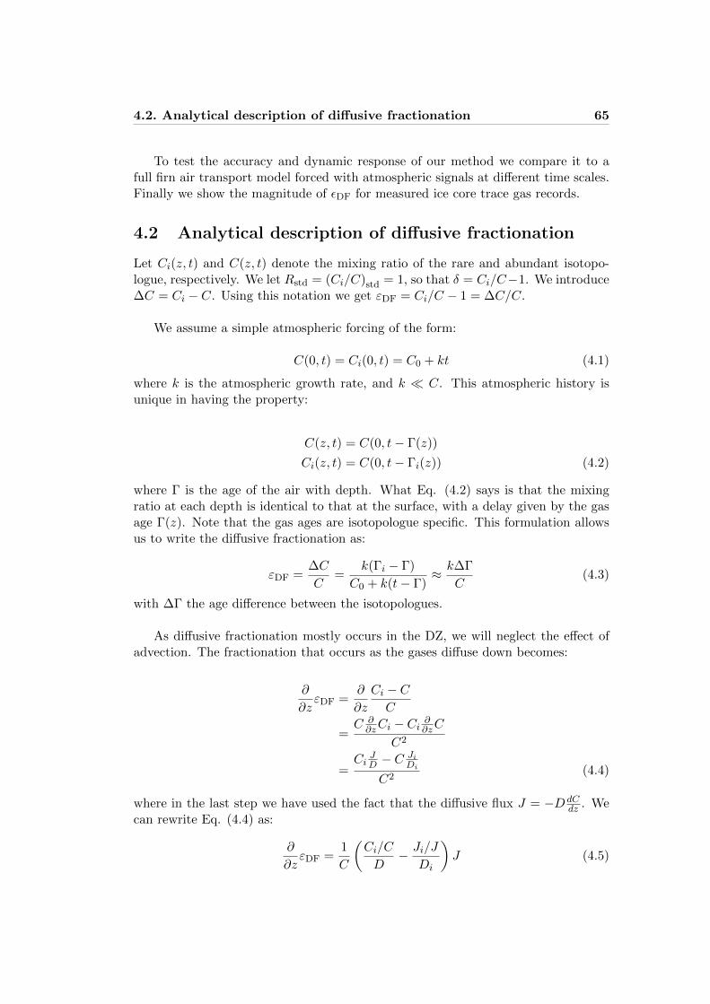
4.2. Analytical description of diffusive fractionation 65

To test the accuracy and dynamic response of our method we compare it to afull firn air transport model forced with atmospheric signals at different time scales.Finally we show the magnitude of εDF for measured ice core trace gas records.

4.2 Analytical description of diffusive fractionation

Let Ci(z, t) and C(z, t) denote the mixing ratio of the rare and abundant isotopo-logue, respectively. We let Rstd = (Ci/C)std = 1, so that δ = Ci/C−1. We introduce∆C = Ci − C. Using this notation we get εDF = Ci/C − 1 = ∆C/C.

We assume a simple atmospheric forcing of the form:

C(0, t) = Ci(0, t) = C0 + kt (4.1)

where k is the atmospheric growth rate, and k � C. This atmospheric history isunique in having the property:

C(z, t) = C(0, t− Γ(z))

Ci(z, t) = C(0, t− Γi(z)) (4.2)

where Γ is the age of the air with depth. What Eq. (4.2) says is that the mixingratio at each depth is identical to that at the surface, with a delay given by the gasage Γ(z). Note that the gas ages are isotopologue specific. This formulation allowsus to write the diffusive fractionation as:

εDF =∆C

C=

k(Γi − Γ)

C0 + k(t− Γ)≈ k∆Γ

C(4.3)

with ∆Γ the age difference between the isotopologues.

As diffusive fractionation mostly occurs in the DZ, we will neglect the effect ofadvection. The fractionation that occurs as the gases diffuse down becomes:

∂

∂zεDF =

∂

∂z

Ci − CC

=C ∂∂zCi − Ci

∂∂zC

C2

=Ci

JD − C

JiDi

C2(4.4)

where in the last step we have used the fact that the diffusive flux J = −D dCdz . We

can rewrite Eq. (4.4) as:

∂

∂zεDF =

1

C

(Ci/C

D− Ji/J

Di

)J (4.5)

66 Chapter 4. Diffusive fractionation in the firn

because CiC ≈

JiJ ≈ 1 we can simplify to:

∂

∂zεDF =

1

C

(1

D− 1

Di

)J =

1

C

(D

Di− 1

)∂C

∂z(4.6)

using the fact that ∂C∂z = −k ∂Γ

∂z , we find:

∂

∂zεDF = − k

C

(D

Di− 1

)∂Γ

∂z

and

εDF(z) ≈ − kC

(D

Di− 1

)Γ(z) (4.7)

From Eq. 4.7 we can draw a number of interesting conclusions:

• It is not the increase k itself that matters, but rather the relative increase k/C.For an exponential atmospheric increase (constant k/C), the DF in the firn isconstant with time.

• The DF scales linearly with (D/Di − 1). This quantity is shown in Table 4.1for several trace gases relevant to ice core studies. The effect is largest forlight gases such as methane and H2. Because the molecules are relatively light(MCH4 = 16.04 kg mol−1 and MH2 = 2.02 kg mol−1), the isotopic substitutionof 13C (D, i.e. 2H) for 12C (H) makes a large difference for the mass ratio, andthereby the diffusivity ratio.

• The DF scales linearly with the age of the gas. The gas age at the firn-icetransition, where the air is trapped, depends strongly on the length of the firncolumn. The DF is larger in the deep firns of the Antarctic plateau than inthe shallow firns of the (warmer) Antarctic coastal and Greenlandic sites.

• As both isotopologues diffusive through the same firn column, the exact shapeof the depth-diffusivity profile (i.e. the tortuosity) does not matter. The ratioof molecular diffusivities is constant throughout the firn column.

The result of Eq. 4.7 is valid only in the diffusive zone (DZ) where advection isnegligible. In the lock-in zone (LIZ) advection dominates the transport. Advectiondoes not discriminate between isotopologues, giving no continued fractionation withdepth. For this reason the fractionation εDF along the firn whole column is wellapproximated by

εDF =

−kC

(DDi− 1)

Γ(z) for z ≤ zlid

− kC

(DDi− 1)

Γ(zlid) for z > zlid

(4.8)

with zlid the lock-in depth which separates the DZ and LIZ.

4.3. Parameterizing gas age at the lock-in depth 67

Table 4.1: Diffusivity ratios of isotopologues following Buizert et al. (2011) and Trudinger et al.(1997). If the atom mass is not specified, is represents the average weight (i.e. the sum of theisotopic masses multiplied by their relative abundance).

Isotopologue ratio a(DDi

− 1)

b(DDi

− 1)

HH/HD 20.50 × 10−2 -

12CH4/13CH4 1.95 × 10−2 1.79 × 10−2

CH4/CH3D 1.96 × 10−2 -

12CO/13CO 0.89 × 10−2 -C16O/C18O 1.74 × 10−2 -

12CO2/13CO2 0.44 × 10−2 0.42 × 10−2

CO2/14CO2 0.87 × 10−2 0.83 × 10−2

C16O16O/C18O16O 0.88 × 10−2 -

14N14NO/15N14NO 0.44 × 10−2 -NN16O/NN18O 0.88 × 10−2 -a Buizert et al. (2011)b Trudinger et al. (1997)

In deriving Eq. 4.8 we made some assumptions and simplifications. To verifyits correctness we now compare the analytical result to the modeled DF at NEEMfor six firn air transport models (synthetic scenario I in section 3.4.4). The scenarioconsists of a hypothetical monotonic CO2 increase following:

[12CO2] = [13CO2] = 225 exp[2.5× 10−3(t− 1800)

]ppm (4.9)

with t the time in years C.E. Equation (4.9) corresponds to a constant k/C =2.5× 10−3. The final decimal model date is 2008.54, corresponding to the samplingdate at NEEM. For the mean age Γ(z) we use the first moment of the NEEM CO2

age distribution G(z, t) calculated with the CIC firn air model:

Γ(z) =

∫ ∞0

G(z, t)× t dt (4.10)

The modeled solutions are compared to the analytical result in Fig. 4.2. We findthat within the DZ the models and the analytical result agree very well. Within theLIZ the model solutions diverge strongly, as discussed in detail in section 3.4.4. Theanalytical solution falls within the spread observed among the models. From thiswe can conclude that Eq. 4.8 gives an accurate prediction of the diffusive isotopicfractionation in the firn.

4.3 Parameterizing gas age at the lock-in depth

Equation (4.8) in principle allows us to calculate εDF in the ice core record in or-der to correct isotopic measurements. The values of C and k can be derived from

68 Chapter 4. Diffusive fractionation in the firn

LIZDZ

−0.15 −0.1 −0.05 0

70

60

50

40

30

20

10

0

εDF

/ δ13CO2 (‰)

Dep

th (

m)

CICCSIROINSTAARLGGE−GIPSAOSUSIOAnalytical

Figure 4.2: Isotopic diffusive fractionation in the NEEM firn for a hypothetical atmospheric CO2

scenario. See section 3.3.2 for model acronyms and details.

Table 4.2: Overview of firn air sites used in the gas age parameterization. See Table 2.1 for moredetails.

Site p T A DCH Year(hPa) (◦C) (cm ice yr−1) (m) sampled

NEEM 745 -28.9 22 59.8 2008NGRIP 691 -31.1 19 66.5 2001

Berkner Island 895 -26 13 50.0 2003Dome C 658 -54 3.2 93.0 1999South Pole 681 -51 8 115.0 1995

measured trace gas mixing ratios, the mean age Γ is the only unknown. Here wederive a parameterization of Γ(zlid), i.e. the mean gas age at the lock-in depth.Since the vast majority of the air is occluded within the LIZ (∼ 95% at NEEM),the value of εDF at the lock-in depth gives a good estimate of εDF recorded in the ice.

We tuned the CIC firn air model (Chapter 5) to five modern firn air sites rep-resenting both hemispheres and a wide range of climatic conditions. The sites aresummarized in Table 4.2. For each site we reconstructed the diffusivity-depth profileusing reference tracers of known atmospheric history (see Sections 2.5.1, 3.3.1 and5.6). For this purpose the lock-in depth is chosen as the depth where the tortuosityof the pore geometry reduces the effective diffusivity by three orders of magnitudebelow the free air diffusivity; this is generally equal to the depth where gravitational

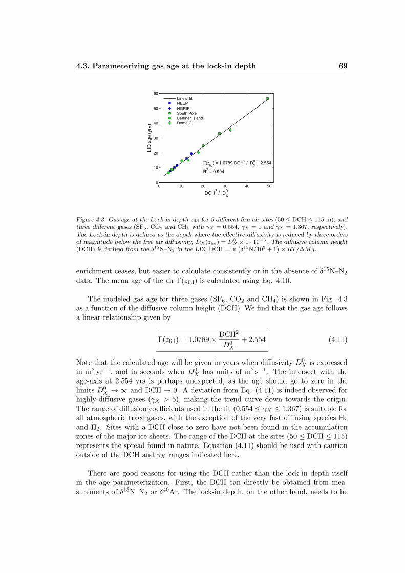
4.3. Parameterizing gas age at the lock-in depth 69

0 10 20 30 40 500

10

20

30

40

50

60

DCH2 / D0X

LID

age

(yr

s)

Γ(zlid

) = 1.0789 DCH2 / D0X + 2.554

R2 = 0.994

Linear fitNEEMNGRIPSouth PoleBerkner IslandDome C

Figure 4.3: Gas age at the Lock-in depth zlid for 5 different firn air sites (50 ≤ DCH ≤ 115 m), andthree different gases (SF6, CO2 and CH4 with γX = 0.554, γX = 1 and γX = 1.367, respectively).The Lock-in depth is defined as the depth where the effective diffusivity is reduced by three ordersof magnitude below the free air diffusivity, DX(zlid) = D0

X × 1 · 10−3. The diffusive column height(DCH) is derived from the δ15N–N2 in the LIZ, DCH = ln

(δ15N/103 + 1

)×RT/∆Mg.

enrichment ceases, but easier to calculate consistently or in the absence of δ15N–N2

data. The mean age of the air Γ(zlid) is calculated using Eq. 4.10.

The modeled gas age for three gases (SF6, CO2 and CH4) is shown in Fig. 4.3as a function of the diffusive column height (DCH). We find that the gas age followsa linear relationship given by

Γ(zlid) = 1.0789× DCH2

D0X

+ 2.554 (4.11)

Note that the calculated age will be given in years when diffusivity D0X is expressed

in m2 yr−1, and in seconds when D0X has units of m2 s−1. The intersect with the

age-axis at 2.554 yrs is perhaps unexpected, as the age should go to zero in thelimits D0

X →∞ and DCH→ 0. A deviation from Eq. (4.11) is indeed observed forhighly-diffusive gases (γX > 5), making the trend curve down towards the origin.The range of diffusion coefficients used in the fit (0.554 ≤ γX ≤ 1.367) is suitable forall atmospheric trace gases, with the exception of the very fast diffusing species Heand H2. Sites with a DCH close to zero have not been found in the accumulationzones of the major ice sheets. The range of the DCH at the sites (50 ≤ DCH ≤ 115)represents the spread found in nature. Equation (4.11) should be used with cautionoutside of the DCH and γX ranges indicated here.

There are good reasons for using the DCH rather than the lock-in depth itselfin the age parameterization. First, the DCH can directly be obtained from mea-surements of δ15N–N2 or δ40Ar. The lock-in depth, on the other hand, needs to be

70 Chapter 4. Diffusive fractionation in the firn

−50 0 50

−0.6

−0.4

−0.2

0

−50 0 50

−4

−3

−2

−1

0

Time (yr)

−50 0 50

−0.6

−0.4

−0.2

0

−50 0 50

−4

−3

−2

−1

0

Time (yr)

−100 0 100

−0.2

−0.1

0

−100 0 100

−1

−0.5

0

Time (yr)

−600 0 600

−0.02

−0.01

0

−600 0 600

−0.15

−0.1

−0.05

0

Time (yr)

−50 0 50

−0.04

−0.02

0

0.02

0.04

−50 0 50

−0.2

0

0.2

Time (yr)

−50 0 50

−0.2

0

0.2

−50 0 50

−2

−1

0

1

2

Time (yr)

−150 0 150

−0.2

0

0.2

−150 0 150

−2

−1

0

1

2

Time (yr)

−1000 0 1000

−0.02

0

0.02

−1000 0 1000

−0.2

−0.1

0

0.1

0.2

Time (yr)

CO

2 / C

H4

δ13C

O2 (

‰)

δ13C

H4 (

‰)

CO

2 / C

H4

δ13C

O2 (

‰)

δ13C

H4 (

‰)

1 year 10 years 100 years 1000 years

1 year 10 years 100 years 1000 years

c1

c1

c1

c1

c0

c0

c0

c0

c1

c1

c1

c1

c0

c0

c0

c0

a)

b)

NEEM, Greenland

Figure 4.4: Accuracy and dynamic response of the method compared to the CIC firn air model forthe NEEM site in Greenland. The upper panels show the atmospheric forcing in black, and thecorresponding signal recorded in the ice core in blue (green) for CO2 (CH4). The middle (lower)panels give the DF for δ13CO2 (δ13CH4), where the CIC output is given as a solid curve. Theshading represents the spread in LIZ model solutions observed in the NEEM model intercomparisonof Fig. 4.2. The dashed black line shows the result from Eqs (4.7) and (4.11). (a) Response to alinear ramp from c0 = 190 (400) to c1 = 270 (700) for CO2 (CH4) Duration indicated above. (b)Response to a Gaussian perturbation of indicated 2σ width.

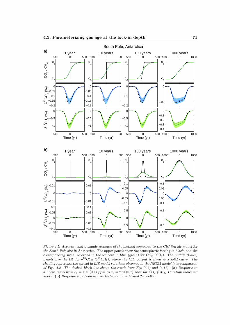
4.3. Parameterizing gas age at the lock-in depth 71

−500 0 500

−0.2

−0.15

−0.1

−0.05

0

−500 0 500

−1

−0.5

0

Time (yr)

−500 0 500

−0.2

−0.15

−0.1

−0.05

0

−500 0 500

−1

−0.5

0

Time (yr)

−500 0 500

−0.2

−0.1

0

−500 0 500

−1

−0.5

0

Time (yr)

−1000 0 1000

−0.05

0

−1000 0 1000

−0.4

−0.3

−0.2

−0.1

0

Time (yr)

−500 0 500

−0.01

0

0.01

−500 0 500−0.1

−0.05

0

0.05

0.1

Time (yr)

−500 0 500

−0.01

0

0.01

−500 0 500−0.1

−0.05

0

0.05

0.1

Time (yr)

−500 0 500

−0.1

−0.05

0

0.05

0.1

−500 0 500

−0.5

0

0.5

Time (yr)

−1000 0 1000

−0.1

−0.05

0

0.05

0.1

−1000 0 1000

−0.5

0

0.5

Time (yr)

CO

2 / C

H4

δ13C

O2 (

‰)

δ13C

H4 (

‰)

CO

2 / C

H4

δ13C

O2 (

‰)

δ13C

H4 (

‰)

1 year 10 years 100 years 1000 years

1 year 10 years 100 years 1000 years

c1

c1

c1

c1

c0

c0

c0

c0

c1

c1

c1

c1

c0

c0

c0

c0

a)

b)

South Pole, Antarctica

Figure 4.5: Accuracy and dynamic response of the method compared to the CIC firn air model forthe South Pole site in Antarctica. The upper panels show the atmospheric forcing in black, and thecorresponding signal recorded in the ice core in blue (green) for CO2 (CH4). The middle (lower)panels give the DF for δ13CO2 (δ13CH4), where the CIC output is given as a solid curve. Theshading represents the spread in LIZ model solutions observed in the NEEM model intercomparisonof Fig. 4.2. The dashed black line shows the result from Eqs (4.7) and (4.11). (a) Response toa linear ramp from c0 = 190 (0.4) ppm to c1 = 270 (0.7) ppm for CO2 (CH4) Duration indicatedabove. (b) Response to a Gaussian perturbation of indicated 2σ width.

72 Chapter 4. Diffusive fractionation in the firn

reconstructed using firn densification models, which are laborious, have inherent un-certainties, and show a pronounced mismatch with experimental data for the glacialperiod in Antarctic ice cores (Landais et al., 2006). Second, due to vigorous ventila-tion, air at the bottom of the CZ is effectively of modern composition, i.e. has a gasage of zero. The gas ages within the DZ, and therefore the gas age at zlid dependsmostly on the DCH.

The age parameterization of Eq. (4.11) can also be used when modeling ∆ageback in time with densification models. The ice age is calculated with the firn densi-fication model, yet to obtain ∆age the gas age should be subtracted. As the detailsof the diffusivity-depth profile are unknown, Eq. (4.11) can be used to calculate theage based on the DCH alone.

4.4 Diffusive fractionation in the ice core record

4.4.1 Comparison to the CIC firn air model

To test the accuracy and dynamic response of our method we compare it the out-put of the full CIC firn air model for a number of scenarios. First, we use a ramp,where the atmospheric mixing ratio increases linearly from c0 = 190 (0.40) ppmto c1 = 270 (0.70) ppm for CO2 (CH4). These values were chosen to representthe glacial-interglacial natural variability range of both gases. To test the dynamicresponse of our method the duration of the ramp is varied over three orders of mag-nitude from 1, 10, 100 to 1000 years. Second, we use a Gaussian bell curve, wherethe atmospheric mixing ratio changes from c0 to c1. The 2σ width is varied from 1,10, 100 to 1000 years.

The results for NEEM and South Pole are shown in Figures 4.4 and 4.5, respec-tively. The upper row of panels each time shows the atmospheric forcing in black,with the CO2 (CH4) signal as recorded in the ice core in blue (green). Note that theblue line line is often not visible as the green line is plotted on top of it. The middle(lower) row of panels shows the resulting DF for δ13CO2 (δ13CH4). The CIC modelresult is plotted as a solid line, with a shaded area around it representing the DFmodel spread observed in the NEEM model intercomparison study (section 3.4.4).We let the model calculate the mixing ratios in the closed bubbles (section 5.7). Ourempirical method, consisting of Eqs. (4.7) and (4.11), is plotted as a dashed blackline. In Eq. (4.7) we use k = dC/dt and C from the signals that would be recordedin the ice core, rather than the original atmospheric forcing. This is more realistic,as this would be the data available from real ice cores.

We find that our method agrees very well with the full model results over awide range of time scales as well as for completely different firn air sites. For rapidsignals (1,10 years) there appears to be a timing difference of a few years between ourmethod and the full model results. Note that these rapid cases are mostly academic,

4.4. Diffusive fractionation in the ice core record 73

as such rapid variations are not observed in the ice core record. For processes onlonger, more realistic time scales (100, 1000 years) the timing offset is negligible.As noted above, in our empirical method we use the smoothed concentrations asrecorded in the ice rather than the original atmospheric variations. As it turns out,this gives better results. The reason is that the DF signal and the trace gas mixingratios are smoothed to the same degree by both firn diffusion and bubble trapping.This is a major advantage of our new method; in a full model effort to calculateεDF, one would first need to reconstruct the original atmospheric variations (Spahniet al., 2003; Kohler et al., 2011).

Apart from the minor timing issue for rapid variations, our method gives resultsthat fall within the shaded areas that represent the model uncertainty. Generallyour method gives a slightly lower isotopic fractionation than the CIC model does.This is to be expected from the firn column comparison shown in Fig. 4.2.

4.4.2 DF in the ice core gas record

We will now apply our method to ice core measurements, and calculate εDF for pastatmospheric variations. The results are shown in Figs. 4.6 and 4.7, for Greenland(GISP2 and NGRIP) and Antarctica (EPICA Dome C), respectively. For Greenlandwe consider fractionation of CH4 isotopologues only. Due to the presence of CO2

artifacts, there is no reliable northern hemisphere CO2 record from Greenland (e.g.Tschumi and Stauffer, 2000).

The fractionation εDF is calculated in three steps. First, we calculate the DCHfrom the gravitational signal shown in Fig. 4.6c (4.7d). Second, we insert the DCHin Eq. (4.11) and obtain the mean gas age at the lock-in depth, shown in Fig. 4.6d(4.7e). Last, this mean age Γ is used in Eq. (4.7) together with the derivative of themeasured mixing ratios to calculate εDF. The result is shown in Fig. 4.6e (4.7f-g),note that the scale has been inverted. The εDF calculated for CH4 applies to both δDand δ13C , since they have essentially the same isotopologue diffusivity ratio (Table4.1). In section 4.5 we will discuss the uncertainties of the method, as well as theimplications of our results.

4.4.3 Correcting δ13C–CH4 data for DF

Finally we look at published records of δ13C–CH4 over the last glacial termination(Fischer et al., 2008) and the 8.2 kyr event (Sowers, 2010), and correct them for theeffect of DF. For the last termination the results are shown in Fig. 4.8c, with theoriginal (uncorrected) data in blue and the DF corrected data in orange (with er-rorbar). Note that the isotopic scale has been inverted. During each rapid variationin atmospheric CH4 concentration (indicated by the grey bars) we find a substantialDF signal. For these three transitions the correction ranged from 0.30–0.53 h, morethan double the analytical precision of 0.15 h in the study. The errorbars on the

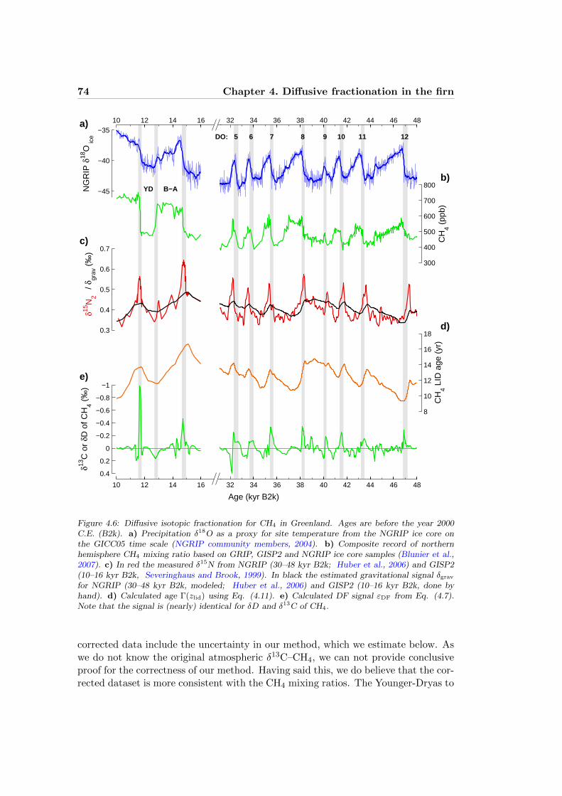
74 Chapter 4. Diffusive fractionation in the firn

10 12 14 16

10 12 14 16

32 34 36 38 40 42 44 46 48

32 34 36 38 40 42 44 46 48

−45

−40

−35

NG

RIP

δ18

O ic

e

300

400

500

600

700

800

CH

4 (pp

b)

0.3

0.4

0.5

0.6

0.7

/

δ grav

(‰

)

8

10

12

14

16

18

CH

4 LID

age

(yr

)

0.4

0.2

0

−0.2

−0.4

−0.6

−0.8

−1

δ13C

or

δD o

f CH

4 (‰

)δ15

N2

Age (kyr B2k)

a)

b)

c)

d)

e)

DO: 5 6 7 8 9 10 11 12

YD B−A

Figure 4.6: Diffusive isotopic fractionation for CH4 in Greenland. Ages are before the year 2000C.E. (B2k). a) Precipitation δ18O as a proxy for site temperature from the NGRIP ice core onthe GICC05 time scale (NGRIP community members, 2004). b) Composite record of northernhemisphere CH4 mixing ratio based on GRIP, GISP2 and NGRIP ice core samples (Blunier et al.,2007). c) In red the measured δ15N from NGRIP (30–48 kyr B2k; Huber et al., 2006) and GISP2(10–16 kyr B2k, Severinghaus and Brook, 1999). In black the estimated gravitational signal δgrav

for NGRIP (30–48 kyr B2k, modeled; Huber et al., 2006) and GISP2 (10–16 kyr B2k, done byhand). d) Calculated age Γ(zlid) using Eq. (4.11). e) Calculated DF signal εDF from Eq. (4.7).Note that the signal is (nearly) identical for δD and δ13C of CH4.

corrected data include the uncertainty in our method, which we estimate below. Aswe do not know the original atmospheric δ13C–CH4, we can not provide conclusiveproof for the correctness of our method. Having said this, we do believe that the cor-rected dataset is more consistent with the CH4 mixing ratios. The Younger-Dryas to

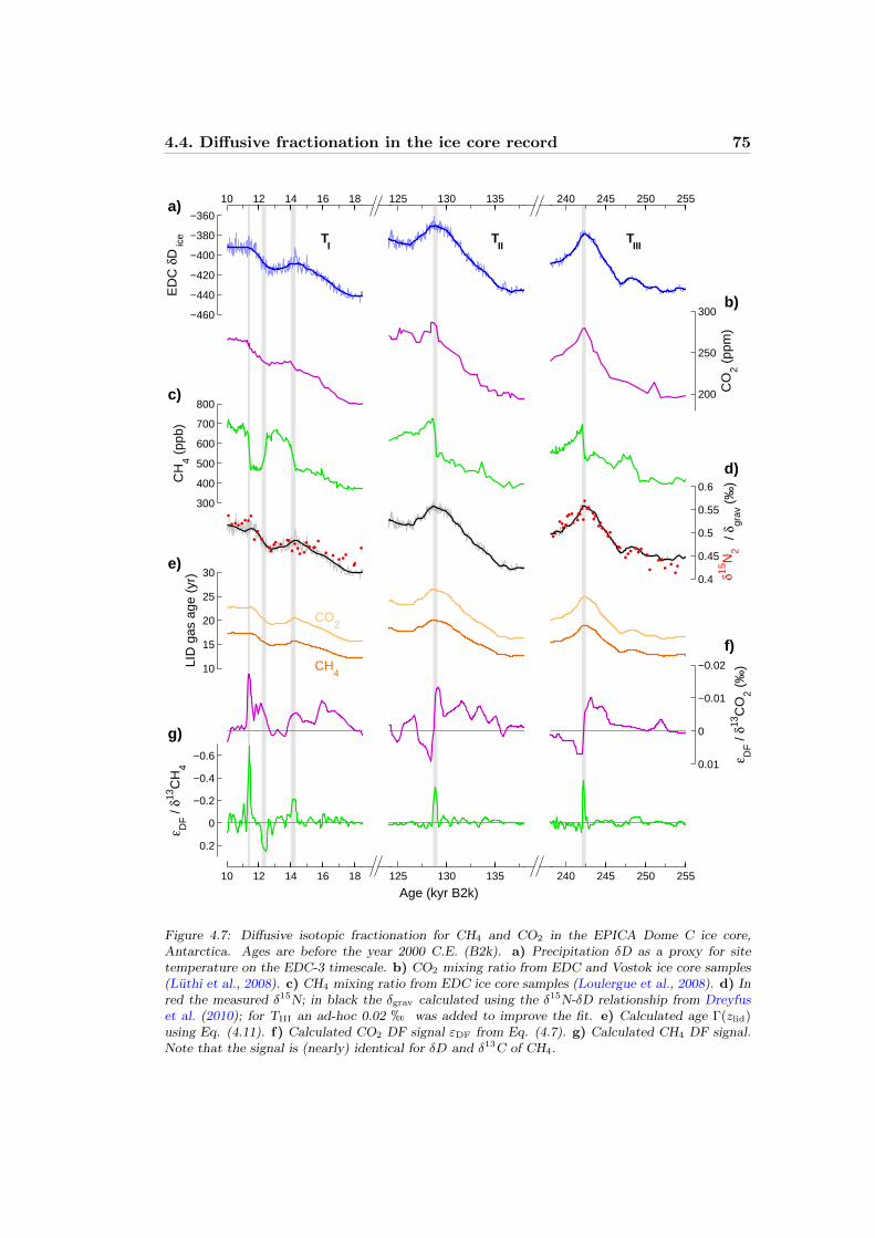
4.4. Diffusive fractionation in the ice core record 75

10 12 14 16 18

10 12 14 16 18

125 130 135

125 130 135

240 245 250 255

240 245 250 255

−460

−440

−420

−400

−380

−360

ED

C δ

D ic

e

200

250

300

CO

2 (pp

m)

300

400

500

600

700

800

CH

4 (pp

b)

0.4

0.45

0.5

0.55

0.6

/ δgr

av (

‰)

10

15

20

25

30

LID

gas

age

(yr

)

CH4

CO2

0.01

0

−0.01

−0.02

ε DF /

δ13C

O2 (

‰)

0.2

0

−0.2

−0.4

−0.6

ε DF /

δ13C

H4

δ15N

2

Age (kyr B2k)

a)

b)

c)

d)

e)

f)

g)

TI

TII

TIII

Figure 4.7: Diffusive isotopic fractionation for CH4 and CO2 in the EPICA Dome C ice core,Antarctica. Ages are before the year 2000 C.E. (B2k). a) Precipitation δD as a proxy for sitetemperature on the EDC-3 timescale. b) CO2 mixing ratio from EDC and Vostok ice core samples(Luthi et al., 2008). c) CH4 mixing ratio from EDC ice core samples (Loulergue et al., 2008). d) Inred the measured δ15N; in black the δgrav calculated using the δ15N-δD relationship from Dreyfuset al. (2010); for TIII an ad-hoc 0.02 h was added to improve the fit. e) Calculated age Γ(zlid)using Eq. (4.11). f) Calculated CO2 DF signal εDF from Eq. (4.7). g) Calculated CH4 DF signal.Note that the signal is (nearly) identical for δD and δ13C of CH4.

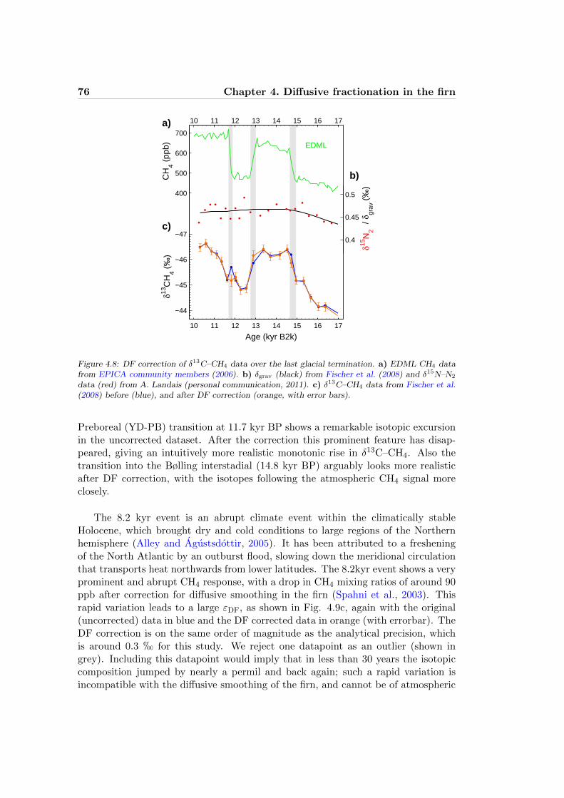
76 Chapter 4. Diffusive fractionation in the firn

10 11 12 13 14 15 16 17

10 11 12 13 14 15 16 17

400

500

600

700

EDML

0.4

0.45

0.5

/ δgr

av (

‰)

−44

−45

−46

−47

δ15N

2

CH

4 (pp

b)δ13

CH

4 (‰

)

Age (kyr B2k)

a)

b)

c)

Figure 4.8: DF correction of δ13C–CH4 data over the last glacial termination. a) EDML CH4 datafrom EPICA community members (2006). b) δgrav (black) from Fischer et al. (2008) and δ15N–N2

data (red) from A. Landais (personal communication, 2011). c) δ13C–CH4 data from Fischer et al.(2008) before (blue), and after DF correction (orange, with error bars).

Preboreal (YD-PB) transition at 11.7 kyr BP shows a remarkable isotopic excursionin the uncorrected dataset. After the correction this prominent feature has disap-peared, giving an intuitively more realistic monotonic rise in δ13C–CH4. Also thetransition into the Bølling interstadial (14.8 kyr BP) arguably looks more realisticafter DF correction, with the isotopes following the atmospheric CH4 signal moreclosely.

The 8.2 kyr event is an abrupt climate event within the climatically stableHolocene, which brought dry and cold conditions to large regions of the Northernhemisphere (Alley and Agustsdottir, 2005). It has been attributed to a fresheningof the North Atlantic by an outburst flood, slowing down the meridional circulationthat transports heat northwards from lower latitudes. The 8.2kyr event shows a veryprominent and abrupt CH4 response, with a drop in CH4 mixing ratios of around 90ppb after correction for diffusive smoothing in the firn (Spahni et al., 2003). Thisrapid variation leads to a large εDF, as shown in Fig. 4.9c, again with the original(uncorrected) data in blue and the DF corrected data in orange (with errorbar). TheDF correction is on the same order of magnitude as the analytical precision, whichis around 0.3 h for this study. We reject one datapoint as an outlier (shown ingrey). Including this datapoint would imply that in less than 30 years the isotopiccomposition jumped by nearly a permil and back again; such a rapid variation isincompatible with the diffusive smoothing of the firn, and cannot be of atmospheric

4.5. Discussion 77

8 8.1 8.2 8.3 8.4 8.5

8 8.1 8.2 8.3 8.4 8.5

550

600

650

700

GISP2

0.25

0.3

0.35

/ δgr

av (

‰)

−46

−47

−48 δ15N

2

CH

4 (pp

b)δ13

CH

4 (‰

)

Age (kyr B2k)

a)

b)

c)

Figure 4.9: DF correction of δ13C–CH4 data over the 8.2 kyr event. a) High resolution GISP2 CH4

and b) δ15N–N2 data from Kobashi et al. (2007). The plotted δgrav signal (in black) is a quadraticfit to the reconstructed δgrav based on δ15Nexcess = δ15N−δ40Ar/4. c) δ13C–CH4 data from Sowers(2010) before (blue), and after DF correction (orange, with error bars).

origin.

After correction we observe an enrichment in δ13C–CH4 for the duration of theevent, which hints at reduced wetland emissions in a colder/dryer Northern hemi-sphere climate. The δ13C–CH4 signal appears to have the right order of magnitude:∼0.6 h for a 75 ppb drop in CH4, compared to a 1.5 h signal for the 180 ppb dropfrom the Allerød to the YD. Both these NH cold spells are thought to be triggeredby the same mechanism, and we could expect to see a similar response in the CH4

isotopic composition. Again, we cannot verify the correctness of our DF correctionmethod, as we do not posses knowledge of the true atmospheric history. However, anenrichment of more modest amplitude that persists throughout the event seems moreplausible than the two separated, high amplitude excursions found in the uncorrectedtime series.

4.5 Discussion

4.5.1 Relevance of the DF correction

In principle, all ice core records of trace gas isotopic composition should be correctedfor the effect of DF. Whether this correction is relevant depends on the magnitude ofεDF compared to 1) the analytical precision of the ice core measurements of trace gasisotopes, 2) the magnitude and uncertainty of the applied gravitational correction,

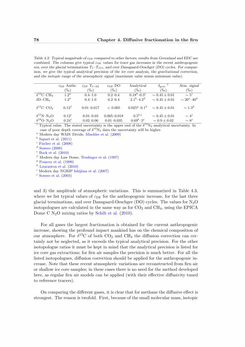
78 Chapter 4. Diffusive fractionation in the firn

Table 4.3: Typical magnitude of εDF compared to other factors; results from Greenland and EDC arecombined. The columns give typical εDF values for trace gas increases in the recent anthropogenicera, over the glacial terminations TI–TIII , and over Dansgaard-Oeschger (DO) cycles. For compar-ison, we give the typical analytical precision of the ice core analysis, the gravitational correction,and the isotopic range of the atmospheric signal (maximum value minus minimum value).

εDF Anthr. εDF TI−III εDF DO Analytical δgrav† Atm. signal

(h) (h) (h) (h) (h) (h)

δ13C–CH4 1.2a 0.4–1.0 0.2–0.4 0.18b–0.3c ∼ 0.45 ± 0.01 ∼ 5c

δD–CH4 1.2a 0.4–1.0 0.2–0.4 2.1b–4.2d ∼ 0.45 ± 0.01 ∼ 20e–40d

δ13C–CO2 0.12f 0.01–0.017 < 0.005 0.025g–0.1h ∼ 0.45 ± 0.01 ∼ 1.3h

δ15N–N2O 0.12i 0.01–0.03 0.005–0.018 0.5b,j ∼ 0.45 ± 0.01 ∼ 4j

δ18O–N2O 0.24i 0.02–0.06 0.01–0.035 0.69b–2j ∼ 0.9 ± 0.02 ∼ 8j

† Typical value. The stated uncertainty is the upper end of the δ15N2 analytical uncertainty. Incase of poor depth coverage of δ15N2 data the uncertainty will be higher.

a Modern day WAIS–Divide, Mischler et al. (2009)b Sapart et al. (2011)c Fischer et al. (2008)d Sowers (2006)e Bock et al. (2010)f Modern day Law Dome, Trudinger et al. (1997)g Francey et al. (1999)h Lourantou et al. (2010)i Modern day NGRIP Ishijima et al. (2007)j Sowers et al. (2003)

and 3) the amplitude of atmospheric variations. This is summarized in Table 4.3,where we list typical values of εDF for the anthropogenic increase, for the last threeglacial terminations, and over Dansgaard-Oeschger (DO) cycles. The values for N2Oisotopologues are calculated in the same way as for CO2 and CH4, using the EPICADome C N2O mixing ratios by Schilt et al. (2010).

For all gases the largest fractionation is obtained for the current anthropogenicincrease, showing the profound impact mankind has on the chemical composition ofour atmosphere. For δ13C of both CO2 and CH4 the diffusion correction can cer-tainly not be neglected, as it exceeds the typical analytical precision. For the otherisotopologue ratios it must be kept in mind that the analytical precision is listed forice core gas extractions; for firn air samples the precision is much better. For all thelisted isotopologues, diffusion correction should be applied for the anthropogenic in-crease. Note that these recent atmospheric variations are reconstructed from firn airor shallow ice core samples; in these cases there is no need for the method developedhere, as regular firn air models can be applied (with their effective diffusivity tunedto reference tracers).

On comparing the different gases, it is clear that for methane the diffusive effect isstrongest. The reason is twofold. First, because of the small molecular mass, isotopic

4.5. Discussion 79

substitution has a large impact on the molecular mass and thereby the moleculardiffusivity. This enhances DF, as is evident from Eq. (4.7). Second, because of itsshort atmospheric lifetime of around 8 years (Lelieveld et al., 1998), the CH4 mixingratio can change very rapidly. The methane record shows the most abrupt changesof all atmospheric trace gases. The magnitude of εDF is identical for both δD andδ13C of CH4, yet the relevance is different to both signals. For δ13C the calculatedεDF for both glacial terminations and the DO cycles exceed the typical analyticalprecision. The correction is comparable to, or larger than, the gravitational correc-tion that is routinely applied to the data. Therefore DF correction of δ13C–CH4 isrecommended for samples that lie within climatic transitions. For δD–CH4 the situ-ation is different. Although εDF has the same magnitude, it is smaller than both theanalytical measurement precision and the large amplitude of atmospheric variationsobserved in the ice core record (Bock et al., 2010; Sowers, 2006). For these reasonsone could justify omitting the DF correction for δD–CH4.

Nitrous oxide provides a simple case. With the exception of the anthropogenicsignal, the DF correction is more than an order of magnitude smaller than the analyt-ical precision. In most cases εDF is smaller than the uncertainty in the gravitationalcorrection. The effect of DF can safely be ignored for N2O records. The case of CO2

is similar. However, because the analytical precision is so much better for δ13CO2,one could consider applying the DF correction during the deglaciations, which areaccompanied by a strong CO2 increase.

In summary, δ13C–CH4 is the only trace gas isotopic signal for which the DFcorrection should always be applied during transitions, as there the εDF exceeds thetypical experimental precision. For δD–CH4 and δ13C–CO2 the magnitude of εDF

gets to about half the analytical precision only during glacial terminations; one couldconsider DF correction during these special intervals. In all other cases the effectsof DF can safely be neglected.

We believe that the method presented here also has merits in cases where εDF isvery small. Calculating the magnitude of the DF correction is reduced from a mod-eling project to a back-of-the-envelope calculation. This will enable experimentaliststo quickly asses whether they need to worry about DF correcting their data or not.

4.5.2 Accuracy of our method

Here we will estimate the uncertainty in our method. We distinguish three majorsources of uncertainty:

1) The DCH estimate based on δ15N–N2 data. The analytical precisionof the δ15N measurements is on the order of 0.005–0.01 h (Dreyfus et al., 2010);since the depth coverage is not always equally good for each ice core, we estimate theuncertainty at 0.02 h. More problematic is the possibility of thermal fractionation

80 Chapter 4. Diffusive fractionation in the firn

in the firn column caused by temperature gradients (Severinghaus et al., 2001). InGreenland, rapid variations in surface temperature give rise to transient excursionsin δ15N–N2 that do not reflect changes in the DCH (Severinghaus and Brook, 1999).This is shown in Fig. 4.6c, where we plot measured δ15N–N2 data in red, and areconstructed gravitational signal δgrav representing the DCH in black (Huber et al.,2006). In Antarctica temperature variations are too gradual to impose large gradi-ents in the firn. However, during glacial conditions the reduced downward advectionof cold ice (due to low accumulation), in combination with the thermal heat fluxfrom the bed and an increased thermal insulation provided by the deep glacial firncolumn, can lead to a temperature gradient of up to a few K between the surface andthe close-off depth (Goujon et al., 2003). We estimate the error due to the thermalfractionation δtherm from the difference between the apparent and true DCH in theHuber et al. (2006) study, i.e. the red and black curves in 4.6c. We disregard therapid isotope excursions that are easily identified as thermal signals, and take theroot mean square (RMS) of the remaining δtherm dataset. This way we obtain anuncertainty estimate of 0.032 h due to thermal fractionation, leading to a totaluncertainty on δgrav of 0.038 h. Note that this uncertainty can be reduced by ei-ther more advanced experimental methods that require additional δ40Ar and δKr/Armeasurements (Severinghaus et al., 2003), or modeling of heat diffusion in the firnand ice (e.g. Goujon et al., 2003).

2) The uncertainty in firn air model calculations of εDF. Figure 4.2 showsthe disagreement among six firn air models on the magnitude of DF in the LIZ; adisagreement originating from our limited understanding of LIZ transport. This un-certainty also influences the accuracy of our method. The observed model divergencein εDF increases with depth in the LIZ. Therefore the disagreement is much largerin the open pores than in the closed pores, as the trapping process averages overthe entire LIZ. We estimated the 1σ standard deviation in the closed pores in thefollowing way. First we take the standard deviation of the six modeled profiles ateach depth. We multiply these standard deviations by the trapping rate of Eq. (5.8),and integrate this over the firn column. This way we obtain σ = 0.013 h comparedto a total trapped εDF = −0.115 h; i.e. a relative uncertainty of 0.11 (i.e. 11%).

3) The age parameterization of Eq. (4.11). Our lock-in depth age param-eterization provides a surprisingly good fit to the modeled ages, with a coefficientof determination R2 = 0.994. On average the difference between the modeled agesand those predicted by Eq. (4.11) is 0.77 year; a relative error of 0.04. However,Antarctic glacial conditions lie outside the climatic range of modern day firn siteson which the parameterization is based. In particular, the hypothesis of a deepenedconvective zone during Antarctic glacial conditions could significantly influence thefirn transport properties (Landais et al., 2006). It must be noted that the CZ thick-ness has very limited impact on Γ(zlid), as we discussed earlier in section 4.3. SinceEq. (4.11) provides a good fit over a wide range of climatic conditions, we believethat even under Antarctic glacial conditions the error in the age estimation will be

4.5. Discussion 81

small compared to the uncertainties listed under points 1 and 2 above.

Using standard error propagation methods, and assuming all errors to be un-correlated, we get a relative error of around 0.2 (i.e. 20%) in εDF, at a typicalvalue δ15N–N2 = 0.4 h. If more accurate DCH estimates are available (from eitherheat diffusion modeling or additional δ40Ar or δKr/Ar data) the uncertainty in themethed reduces to around 15%.

For the recent anthropogenic increase the DF correction can be performed withgreatest accuracy, as one can use a firn air transport model with the effectivediffusivity-depth relationship tuned to reference tracers of known atmospheric his-tory. In this case the only major uncertainty is the LIZ model disagreement as shownin Fig. 4.2.

In the ice core record the alternative to our DF correction method is a fullmodeling study, in which the coupled heat diffusion and firn densification is modeledfor the past firn column, after which the DF can be calculated in this reconstructedfirn column using a firn air transport model. This approach would only be moreaccurate for point 1) above, since the modeled temperature gradient in the firn allowsfor estimating the true DCH by correcting δ15N data for thermal fractionation.

Apart from the more accurate DCH estimate, a full modeling approach is subjectto many other uncertainties that do not matter to our approach. We list them below,without attempting to estimate their magnitude:

• The firn densification model requires past accumulation and temperature esti-mates as an input, both of which have their uncertainty.

• There is an inherent uncertainty to the densification modeling; e.g. differentmodels can produce close-off depth values that differ by several meters. Un-der Antarctic glacial conditions, densification models systematically predict adeepening of the firn column, whereas δ15N–N2 data show a shortening of theDCH (Landais et al., 2006). The hypothesis of a deepened glacial CZ is ofteninvoked to explain this mismatch, which would require a CZ thickness of up to40 m at Dome Fuji (Severinghaus et al., 2010).

• The close-off and lock-in depths need to be estimated from the density profile.The former is estimated using the parameterization by Martinerie et al. (1994),which is often (slightly) in disagreement with field data from firn samplingcampaigns; the latter is often estimated by the ad-hoc assumption that thelock-in density simply lies 14 kg m−3 below the close-off density (Schwanderet al., 1997; Blunier and Schwander, 2000).

• The effective diffusivity-depth relationship is generally unknown. The bestavailable parameterization by (Schwander, 1989) often gives unsatisfactory re-sults to field data (Fig. 2.5a).

82 Chapter 4. Diffusive fractionation in the firn

• The true atmospheric mixing ratios are unknown; the ice core record is aconvolution of the atmospheric signal with the firn and bubble trapping transferfunctions. The rapid variations that cause the strongest DF are attenuated inthe firn (Spahni et al., 2003; Kohler et al., 2011). By contrast, our empiricalmethod works best when using the mixing ratios as recorded in the ice core(Figs. 4.4 and 4.5).

Considering the above we contend that, compared to a full model approach, ourDF correction method is certainly more accurate whenever good DCH estimatesare available, and probably more accurate whenever the DCH is based directly onδ15N–N2 data uncorrected for thermal fractionation.

4.6 Summary and Conclusions

Fist, we derived an analytical expression for diffusive isotopic fractionation in thefirn column. Second, based on data from five modern firn air sites we derived aparameterization of the mean gas age at the lock-in depth. By combining bothresults we obtain a convenient empirical framework for correcting ice core data forthe effect of diffusive fractionation. The age parameterization can also be used toimprove estimates of ∆age back in time.

We test the accuracy and dynamic response of our method by comparing it toa firn air transport model for two modern, well-characterized firn air sites. Wefind an excellent agreement on timescales relevant for ice core data (≥ 100 years).We apply our method to CH4, CO2 and N2O mixing ratios found in ice cores.We find that δ13C–CH4 is the only trace gas isotopic signal for which the diffusivecorrection should always be applied during transitions, as there the εDF exceeds thetypical experimental precision. For δD–CH4 and δ13C–CO2 the magnitude of thediffusive fractionation gets to about half the analytical precision only during glacialterminations; one could consider data correction during these special intervals. Inall other cases the effects of DF can safely be neglected.

We apply the DF correction to published δ13C–CH4 records over the last glacialtermination and the 8.2 kyr event. In both cases the DF correction exceeds the ana-lytical precision of the data during abrupt transitions. We argue that the correctedtime series are more consistent than the uncorrected ones.

We show that our method has an uncertainty of around 15% in the case thermalfractionation-corrected δ15N–N2 data is used, and around 20% when uncorrectedδ15N–N2 data is used. We argue that our empirical method is more accurate thanthe alternative of a full modeling study.

Our method requires little computational effort and only commonly available icecore data. If offers experimentalists a convenient framework for assessing whethertheir data should be corrected for the effects of diffusive fractionation.

4.7. References 83

4.7 References

Alley, R. B. and Agustsdottir, A. M. (2005). The 8k event: cause and consequences of a majorholocene abrupt climate change. Quaternary Science Reviews, 24(10-11):1123 – 1149.

Barnola, J. M., Pimienta, P., Raynaud, D., and Korotkevich, Y. S. (1991). CO2-climate relationshipas deduced from the Vostok ice core - A reexamination based on new measurements and on areevaluation of the air dating. Tellus B, 43(2):83–90.

Blunier, T. and Schwander, J. (2000). Gas enclosure in ice: age difference and fractionation, pages307–326. Hokkaido University Press, Sapporo.

Blunier, T., Spahni, R., Barnola, J. M., Chappellaz, J., Loulergue, L., and Schwander, J. (2007).Synchronization of ice core records via atmospheric gases. Clim. Past, 3(2):325–330.

Bock, M., Schmitt, J., Behrens, M., Moller, L., Schneider, R., Sapart, C., and Fischer, H. (2010). Agas chromatography/pyrolysis/isotope ratio mass spectrometry system for high-precision delta Dmeasurements of atmospheric methane extracted from ice cores. Rapid Communications in MassSpectrometry, 24(5):621–633.

Buizert, C., Martinerie, P., Petrenko, V. V., Severinghaus, J. P., Trudinger, C. M., Witrant, E.,Rosen, J. L., Orsi, A. J., Rubino, M., Etheridge, D. M., Steele, L. P., Hogan, C., Laube, J. C.,Sturges, W. T., Levchenko, V. A., Smith, A. M., Levin, I., Conway, T. J., Dlugokencky, E. J.,Lang, P. M., Kawamura, K., Jenk, T. M., White, J. W. C., Sowers, T., Schwander, J., and Blunier,T. (2011). Gas transport in firn: multiple-tracer characterisation and model intercomparison forneem, northern greenland. Atmos. Chem. Phys. Discuss., 11:15975–16021.

Dreyfus, G. B., Jouzel, J., Bender, M. L., Landais, A., Masson-Delmotte, V., and Leuenberger, M.(2010). Firn processes and δ15N: potential for a gas-phase climate proxy. Quaternary Sci. Rev.,29(1-2):28–42.

EPICA community members (2006). One-to-one coupling of glacial climate variability in greenlandand antarctica. Nature, 444(7116):195–198.

Fabre, A., Barnola, J. M., Arnaud, L., and Chappellaz, J. (2000). Determination of gas diffusivityin polar firn: Comparison between experimental measurements and inverse modeling. Geophys.Res. Lett., 27(4):557–560.

Fischer, H., Behrens, M., Bock, M., Richter, U., Schmitt, J., Loulergue, L., Chappellaz, J., Spahni,R., Blunier, T., Leuenberger, M., and Stocker, T. F. (2008). Changing boreal methane sourcesand constant biomass burning during the last termination. Nature, 452(7189):864–867.

Francey, R., Allison, C., Etheridge, D., Trudinger, C., Enting, I., Leuenberger, M., Langenfelds, R.,Michel, E., and Steele, L. (1999). A 1000-year high precision record of delta C-13 in atmosphericCO2. Tellus B, 51(2):170–193.

Goujon, C., Barnola, J. M., and Ritz, C. (2003). Modeling the densification of polar firn includingheat diffusion: Application to close-off characteristics and gas isotopic fractionation for Antarcticaand Greenland sites. J. Geophys. Res.-Atm, 108(D24):18.

Huber, C., Leuenberger, M., Spahni, R., Fluckiger, J., Schwander, J., Stocker, T., Johnsen, S.,Landals, A., and Jouzel, J. (2006). Isotope calibrated Greenland temperature record over MarineIsotope Stage 3 and its relation to CH(4). Earth Planet. Sci. Lett., 243(3-4):504–519.

Ishijima, K., Sugawara, S., Kawamura, K., Hashida, G., Morimoto, S., Murayama, S., Aoki, S., andNakazawa, T. (2007). Temporal variations of the atmospheric nitrous oxide concentration andits δ15N and δ18O for the latter half of the 20th century reconstructed from firn air analyses. J.Geophys. Res.-Atm, 112(D3):12.

Kobashi, T., Severinghaus, J. P., Brook, E. J., Barnola, J.-M., and Grachev, A. M. (2007). Precisetiming and characterization of abrupt climate change 8200 years ago from air trapped in polarice. Quat. Sci. Rev., 26(9-10):1212–1222.

Kohler, P., Knorr, G., Buiron, D., Lourantou, A., and Chappellaz, J. (2011). Abrupt rise inatmospheric CO2 at the onset of the Bølling/Allerød: in-situ ice core data versus true atmosphericsignals. Clim. Past., 7(2):473–486.

Landais, A., Barnola, J. M., Kawamura, K., Caillon, N., Delmotte, M., Van Ommen, T., Dreyfus,G., Jouzel, J., Masson-Delmotte, V., Minster, B., Freitag, J., Leuenberger, M., Schwander, J.,Huber, C., Etheridge, D., and Morgan, V. (2006). Firn-air delta N-15 in modern polar sites and

84 Chapter 4. Diffusive fractionation in the firn

glacial-interglacial ice: a model-data mismatch during glacial periods in Antarctica? QuaternarySci. Rev., 25(1-2):49–62.

Lelieveld, J., Crutzen, P. J., and Dentener, F. J. (1998). Changing concentration, lifetime andclimate forcing of atmospheric methane. Tellus B, 50(2):128–150.

Loulergue, L., Schilt, A., Spahni, R., Masson-Delmotte, V., Blunier, T., Lemieux, B., Barnola, J. M.,Raynaud, D., Stocker, T. F., and Chappellaz, J. (2008). Orbital and millennial-scale features ofatmospheric CH4 over the past 800,000 years. Nature, 453(7193):383–386.

Lourantou, A., Chappellaz, J., Barnola, J. M., Masson-Delmotte, V., and Raynaud, D. (2010).Changes in atmospheric CO2 and its carbon isotopic ratio during the penultimate deglaciation.Quaternary Sci. Rev., 29(17-18):1983–1992. doi: DOI: 10.1016/j.quascirev.2010.05.002.

Luthi, D., Le Floch, M., Bereiter, B., Blunier, T., Barnola, J.-M., Siegenthaler, U., Raynaud, D.,Jouzel, J., Fischer, H., Kawamura, K., and Stocker, T. F. (2008). High-resolution carbon dioxideconcentration record 650,000-800,000 years before present. Nature, 453(7193):379–382.

Martinerie, P., Lipenkov, V. Y., Raynaud, D., Chappellaz, J., Barkov, N. I., and Lorius, C. (1994).Air content paleo record in the vostok ice core (antarctica): A mixed record of climatic andglaciological parameters. J. Geophys. Res., 99:10565–10576.

Mischler, J. A., Sowers, T. A., Alley, R. B., Battle, M., McConnell, J. R., Mitchell, L., Popp, T.,Sofen, E., and Spencer, M. K. (2009). Carbon and hydrogen isotopic composition of methaneover the last 1000 years. Global Biogeochem. Cy., 23.

NGRIP community members (2004). High-resolution record of Northern Hemisphere climate ex-tending into the last interglacial period. Nature, 431(7005):147–151.

Sapart, C. J., van der Veen, C., Vigano, I., Brass, M., van de Wal, R. S. W., Bock, M., Fischer,H., Sowers, T., Buizert, C., Sperlich, P., Blunier, T., Behrens, M., Schmitt, J., Seth, B., andRockmann, T. (2011). Simultaneous stable isotope analysis of methane and nitrous oxide on icecore samples. Atmospheric Measurement Techniques Discussions, 4(4):4473–4503.

Schilt, A., Baumgartner, M., Blunier, T., Schwander, J., Spahni, R., Fischer, H., and Stocker, T. F.(2010). Glacialial–interglacial and millennial-scale variations in the atmospheric nitrous oxideconcentration during the last 800,000 years. Quaternary Science Reviews, 29(1-2):182 – 192.

Schwander, J. (1989). The transformation of snow to ice and the occlusion of gases. In Oescher,H. and Langway, C., editors, The Environmental record in glaciers and ice sheets, pages 53–67.John Wiley, New York.

Schwander, J., Sowers, T., Barnola, J. M., Blunier, T., Fuchs, A., and Malaize, B. (1997). Age scaleof the air in the summit ice: Implication for glacial-interglacial temperature change. J. Geophys.Res.-Atm, 102(D16):19483–19493.

Severinghaus, J. P., Albert, M. R., Courville, Z. R., Fahnestock, M. A., Kawamura, K., Montzka,S. A., Muhle, J., Scambos, T. A., Shields, E., Shuman, C. A., Suwa, M., Tans, P., and Weiss,R. F. (2010). Deep air convection in the firn at a zero-accumulation site, central Antarctica.Earth Planet Sc. Lett., 293(3-4):359–367.

Severinghaus, J. P. and Brook, E. J. (1999). Abrupt climate change at the end of the last glacialperiod inferred from trapped air in polar ice. Science, 286(5441):930–934.

Severinghaus, J. P., Grachev, A., and Battle, M. (2001). Thermal fractionation of air in polar firnby seasonal temperature gradients. Geochem. Geophy. Geosy., 2.

Severinghaus, J. P., Grachev, A., Luz, B., and Caillon, N. (2003). A method for precise measurementof argon 40/36 and krypton/argon ratios in trapped air in polar ice with applications to past firnthickness and abrupt climate change in Greenland and at Siple Dome, Antarctica. Geochim.Cosmochim. Ac., 67(3):325–343.

Sowers, T. (2006). Late quaternary atmospheric ch4 isotope record suggests marine clathrates arestable. Science, 311(5762):838–840.

Sowers, T. (2010). Atmospheric methane isotope records covering the holocene period. QuaternarySci. Rev., 29(1-2):213–221. doi: DOI: 10.1016/j.quascirev.2009.05.023.

Sowers, T., Alley, R. B., and Jubenville, J. (2003). Ice Core Records of Atmospheric N2O Coveringthe Last 106,000 Years. Science, 301(5635):945–948.

Spahni, R., Schwander, J., Fluckiger, J., Stauffer, B., Chappellaz, J., and Raynaud, D. (2003). Theattenuation of fast atmospheric ch4 variations recorded in polar ice cores. Geophys. Res. Lett.,

4.7. References 85

30(11):1571.Trudinger, C. M., Enting, I. G., Etheridge, D. M., Francey, R. J., Levchenko, V. A., Steele, L. P.,

Raynaud, D., and Arnaud, L. (1997). Modeling air movement and bubble trapping in firn. J.Geophys. Res.-Atm, 102(D6):6747–6763.

Tschumi, J. and Stauffer, B. (2000). Reconstructing past atmospheric CO2 concentration basedon ice-core analyses: open questions due to in situ production of CO2 in the ice. J. Glaciol.,46(152):45–53.

86 Chapter 4. Diffusive fractionation in the firn

5The CIC firn air model

5.1 Introduction

In this chapter we describe the CIC firn air transport model in detail. In chapter 3 weevaluated the performance of the model for the NEEM site in Northern Greenland,and compared it to other published firn air models. In the comparison we found theperformance to be comparable to, or in some cases better than, other published firnair models.

One of the major differences with other published models (Trudinger et al., 1997;Rommelaere et al., 1997; Sugawara et al., 2003; Severinghaus et al., 2001), is thatwe derive analytical expressions for the air velocity, bubble pressure and trappingrate. The expressions are used to include mass conservation in a rigorous way, andto predict the air content of ice below the firn-ice transition. We furthermore intro-duce a new method to reconstruct the effective diffusivity of the firn using referencetracers of known atmospheric history, and a new way to track the mixing ratio oftrace gases in the closed porosity.

The CIC firn air model is a finite difference 1-D diffusion model coded in MAT-LAB. It uses implicit Crank-Nicholson time stepping to solve what is essentially anadvection-diffusion-reaction equation, with radioactive decay and bubble trappingtaking the place of the chemical reaction by removing trace gas molecules from theopen pore space. The model uses a stationary reference frame with z = 0 at thesurface. The firn column is assumed to be isothermal and in steady state with regardto ice flow and densification rates.

The model includes four types of transport in the open porosity. The first typeis molecular diffusion, which is included through the effective molecular diffusioncoefficient DX, where the X denotes the trace gas under consideration. The secondtype is gravitational settling, which tends to enrich the firn in heavier molecules withdepth (Sowers et al., 1992). The third type is advection, which we include through

87

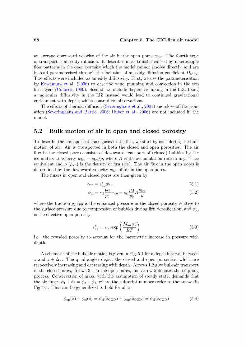
88 Chapter 5. The CIC firn air model

an average downward velocity of the air in the open pores wair. The fourth typeof transport is an eddy diffusion. It describes mass transfer caused by macroscopicflow patterns in the open porosity which the model cannot resolve directly, and areinstead parameterised through the inclusion of an eddy diffusion coefficient Deddy.Two effects were included as an eddy diffusivity. First, we use the parameterisationby Kawamura et al. (2006) to describe wind pumping and convection in the topfirn layers (Colbeck, 1989). Second, we include dispersive mixing in the LIZ. Usinga molecular diffusivity in the LIZ instead would lead to continued gravitationalenrichment with depth, which contradicts observations.

The effects of thermal diffusion (Severinghaus et al., 2001) and close-off fraction-ation (Severinghaus and Battle, 2006; Huber et al., 2006) are not included in themodel.

5.2 Bulk motion of air in open and closed porosity

To describe the transport of trace gases in the firn, we start by considering the bulkmotion of air. Air is transported in both the closed and open porosities. The airflux in the closed pores consists of downward transport of (closed) bubbles by theice matrix at velocity wice = ρice/ρ, where A is the accumulation rate in m yr−1 iceequivalent and ρ (ρice) is the density of firn (ice). The air flux in the open pores isdetermined by the downward velocity wair of air in the open pores.

The fluxes in open and closed pores are then given by

φop = s∗opwair (5.1)

φcl = sclpcl

p0wice = scl

pcl

p0Aρice

ρ(5.2)

where the fraction pcl/p0 is the enhanced pressure in the closed porosity relative tothe surface pressure due to compression of bubbles during firn densification, and s∗op

is the effective open porosity

s∗op = sop exp

(Mairgz

RT

)(5.3)

i.e. the rescaled porosity to account for the barometric increase in pressure withdepth.

A schematic of the bulk air motion is given in Fig. 5.1 for a depth interval betweenz and z + ∆z. The quadrangles depict the closed and open porosities, which arerespectively increasing and decreasing with depth. Arrows 1,2 give bulk air transportin the closed pores, arrows 3,4 in the open pores, and arrow 5 denotes the trappingprocess. Conservation of mass, with the assumption of steady state, demands thatthe air fluxes φ1 + φ3 = φ2 + φ4, where the subscript numbers refer to the arrows inFig. 5.1. This can be generalized to hold for all z:

φop(z) + φcl(z) = φcl(zCOD) + φop(zCOD) = φcl(zCOD) (5.4)

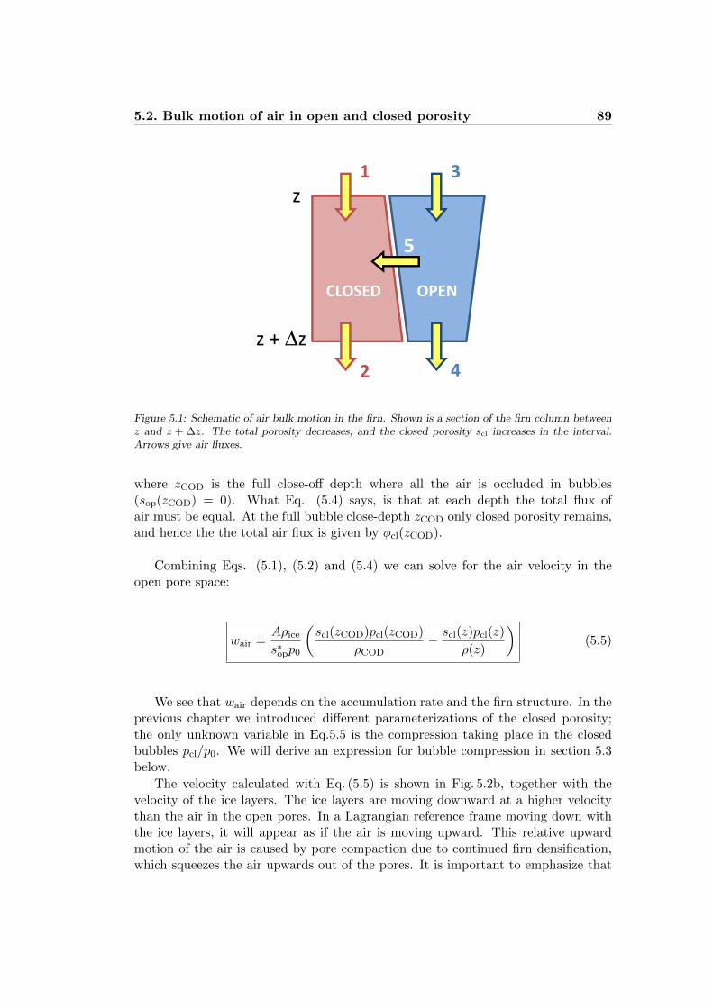
5.2. Bulk motion of air in open and closed porosity 89

z

z + ∆z

OPENCLOSED

1

2

3

4

5

Figure 5.1: Schematic of air bulk motion in the firn. Shown is a section of the firn column betweenz and z + ∆z. The total porosity decreases, and the closed porosity scl increases in the interval.Arrows give air fluxes.

where zCOD is the full close-off depth where all the air is occluded in bubbles(sop(zCOD) = 0). What Eq. (5.4) says, is that at each depth the total flux ofair must be equal. At the full bubble close-depth zCOD only closed porosity remains,and hence the the total air flux is given by φcl(zCOD).

Combining Eqs. (5.1), (5.2) and (5.4) we can solve for the air velocity in theopen pore space:

wair =Aρice

s∗opp0

(scl(zCOD)pcl(zCOD)

ρCOD− scl(z)pcl(z)

ρ(z)

)(5.5)

We see that wair depends on the accumulation rate and the firn structure. In theprevious chapter we introduced different parameterizations of the closed porosity;the only unknown variable in Eq.5.5 is the compression taking place in the closedbubbles pcl/p0. We will derive an expression for bubble compression in section 5.3below.

The velocity calculated with Eq. (5.5) is shown in Fig. 5.2b, together with thevelocity of the ice layers. The ice layers are moving downward at a higher velocitythan the air in the open pores. In a Lagrangian reference frame moving down withthe ice layers, it will appear as if the air is moving upward. This relative upwardmotion of the air is caused by pore compaction due to continued firn densification,which squeezes the air upwards out of the pores. It is important to emphasize that

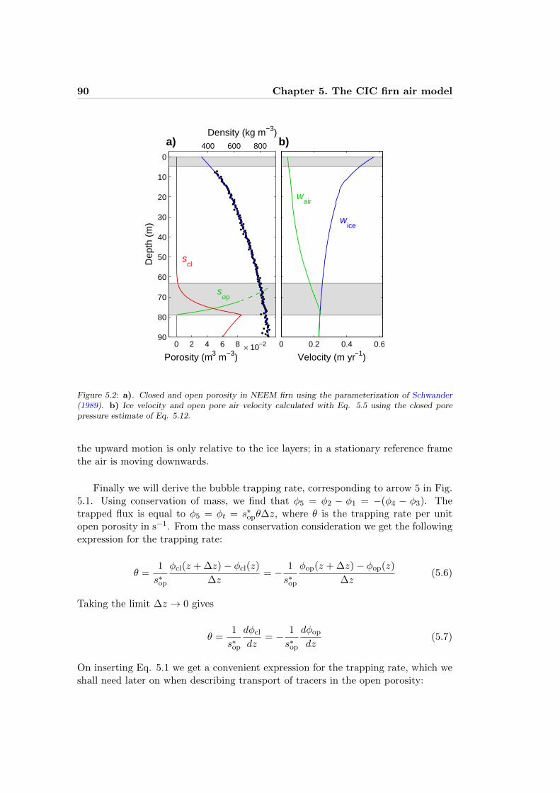
90 Chapter 5. The CIC firn air model

0 0.2 0.4 0.6

Velocity (m yr−1)

400 600 800

Density (kg m−3)

0 2 4 6 890

80

70

60

50

40

30

20

10

0D

epth

(m

)

Porosity (m3 m−3) × 10−2

wair

wice

sop

scl

a) b)

Figure 5.2: a). Closed and open porosity in NEEM firn using the parameterization of Schwander(1989). b) Ice velocity and open pore air velocity calculated with Eq. 5.5 using the closed porepressure estimate of Eq. 5.12.

the upward motion is only relative to the ice layers; in a stationary reference framethe air is moving downwards.

Finally we will derive the bubble trapping rate, corresponding to arrow 5 in Fig.5.1. Using conservation of mass, we find that φ5 = φ2 − φ1 = −(φ4 − φ3). Thetrapped flux is equal to φ5 = φt = s∗opθ∆z, where θ is the trapping rate per unitopen porosity in s−1. From the mass conservation consideration we get the followingexpression for the trapping rate:

θ =1

s∗op

φcl(z + ∆z)− φcl(z)

∆z= − 1

s∗op

φop(z + ∆z)− φop(z)

∆z(5.6)

Taking the limit ∆z → 0 gives

θ =1

s∗op

dφcl

dz= − 1

s∗op

dφop

dz(5.7)

On inserting Eq. 5.1 we get a convenient expression for the trapping rate, which weshall need later on when describing transport of tracers in the open porosity:

5.3. Air pressure in the closed porosity 91

θ = − 1

s∗op

d

dz

(s∗opwair

)(5.8)

5.3 Air pressure in the closed porosity

After a bubble is closed off from the open porosity, the air pressure inside the bubblewill start to increase due to firn densification. Measurements of total air content inmature ice show that more air is occluded than one would get from multiplicationof the porosity at the full close-off depth (zCOD) by the air pressure of the site. Theclose-off fractionation observed for δNe/N2 and δO2/N2, caused by the preferentialexclusion of small molecules from closing bubbles, gives further evidence for an in-creased air pressure in closed bubbles within the LIZ (Severinghaus and Battle, 2006;Huber et al., 2006). Finally, below zCOD increasing bubble pressure is demanded bymass conservation.

The expression for air pressure we derive here is based on two fundamental as-sumptions

1. The firn column is in steady state with respect to accumulation, temperatureand densification rates.

2. The closed pores are compacted at the same rate as the total porosity.

The first assumption is used in all firn air modeling, and is reasonably satisfiedfor the stable climate of the late Holocene. The second assumption is realistic if oneconsiders the following. Firn densification is driven by the hydrostatic pressure ofoverlying precipitation. The vast majority of bubbles are formed within the LIZ, at40-120 m depth. At this depth the overburden pressure that drives densification ison the order of 250-750 kPa. The maximum overpressure in the closed bubbles thatwe find below, is on the order of 20 kPa; i.e. one order of magnitude smaller thanthe overburden pressure. We can therefore reasonably assume that the closed poreswill be compacted at a similar rate to open pores.

We let an imaginary ice parcel sink from depth z′ to depth z, during which thepressure inside a bubble increases from p′ to p. The porosity in the parcel is reducedfrom s(z′) to s(z). However, the porosity is defined as the pore space per unit volume(m3m−3). In the sinking, the parcel gets compacted in the vertical direction by thefirn densification from original length L′ to length L (Fig. 5.3. The new length willbe given by:

92 Chapter 5. The CIC firn air model

L’

L

z’

z

Figure 5.3: An imaginary ice parcel containing air bubbles sinks from depth z′ to depth z.

L = L′ + L′∫dwice

dz′′dt = L′

(1 +

∫d lnwice

)L

L′= 1 + ln

wice(z)

wice(z′)(5.9)

with εzz = dwair/dz the strain rate in the firn. A bubble that is first trapped atdepth z′ will travel down with the ice, and when it reaches depth z its pressure willhave increased by a factor p/p′ that is given by:

p/p′ = ξ(z′, z) =L′s(z′)

Ls(z)=

s(z′)/s(z)

1 + ln [wice(z)/wice(z′)](5.10)

The closed porosity at any given depth z will be a mixture of bubbles trappedalong the depth interval 0 ≤ z′ ≤ z. We can find the average bubble pressure throughintegration. For z ≤ zCOD the mean bubble pressure is given by

pcl(z)

p0=

∫ z

0

dscl

dz′exp

(Mairgz

′

RT

)ξ(z′, z)dz′ (5.11)

and for z > zCOD we get

pcl(z)

p0=pcl(zCOD)

p0ξ(zCOD, z) (5.12)

The average bubble overpressure pcl/(z)p0 is shown in Fig. 5.4b. The average pres-sure does not increase very much with depth, because new bubbles, which are atatmospheric pressure, are continuously added. The addition of new bubbles stops atzCOD (79 m), after which the pressure increases rapidly. In the top ∼ 50 m, thereare essentially no bubbles, however the porosity parameterizations do give a finitevalue for scl. Therefore the calculated bubble pressure at these depths should not

5.3. Air pressure in the closed porosity 93

0 5 10 15 20100

90

80

70

60

50

40

30

20

10

0

Air Flux (L STP m−2 yr−1)

CZ

DZ

LIZ

1 1.5 2 2.5 p / p

0

0 0.1 0.2 0.3100

90

80

70

60

50

40

30

20

10

0

Dep

th (

m)

Porosity (m3 m−3)

sop

scl

pop

pcl

φop

φcl

a) b) c)

Figure 5.4: a). Closed and open porosity in NEEM firn using the parameterization of Goujon et al.(2003). The dashed line gives the total porosity s. b) Pressure in the closed and open porosityrelative to atmosphere (p0). Pressure in the closed bubbles is calculated with Eqs. (5.11) and (5.12);the open porosity follows the barometric pressure increase with depth. c) Air flux in closed andopen pores in liters STP per year per m2. The dashed line gives the total flux.

be trusted. Around 50 m depth the bubble trapping really begins, and the values atthese depths are more realistic.

Inserting the bubble pressure of Eqs. (5.11) and (5.12 and the air velocity of Eq.(5.5) in Eqs. (5.1) and (5.2), we can calculate the air fluxes φop and φcl. This isshown in Fig. 5.4c, using units of L m−2 yr−1 at standard temperature and pres-sure (STP). The total flux is also depicted as the dashed line. Below zCOD the fluxremains constant, as required by mass conservation. This indicates that our descrip-tion of bubble compression gives the right values below the firn-ice transition.

The air flux derived above gives the total air content of ice below the firn-icetransition. The total air content xair can be calculated by:

xair = scl(zCOD)pcl(zCOD)

p0

p0

101325

273.15

T

/ρCOD (5.13)

where xair is the total air content in m3 STP air per kg of ice. For NEEM we modelan air content of 101.0 mL kg−1. This is not far from the true NEEM air content of102 mL kg−1, estimated from mass spectrometer inlet pressures (J. P. Severinghaus,personal communication, 2010). For South Pole, we model an air content of 94.8 mL

94 Chapter 5. The CIC firn air model

kg−1, which is close to the measured value of 92.5 ± 7 mL kg−1 (Martinerie et al.,1992). By contrast, assuming the closed porosity to have the same pressure as theopen porosity, would give a far too low air content of 84.1 (81.2) mL kg−1 at NEEM(South Pole).

Direct measurements of air pressure in the closed firn porosity are very difficult,if not impossible, to achieve. This rules out a direct verification of the equationswe derived here. In our derivation we made only two assumptions, both of whichare realistic. Furthermore, our result (1) gives a physically realistic constant air fluxbelow the LIZ, and (2) accurately predicts the total air content in mature ice for thetwo sites we tested.

5.4 Mass transfer of trace gases

The mathematical description of gas transport is based on Trudinger et al. (1997).The Lagrangian (moving) reference frame is replaced with a Eulerian (static) one,and we explicitly include the air movement and trapping processes we describedabove. We formulate the model in terms of mixing ratios (µmol mol−1, or ppm)rather than concentrations (mol m−3). This enables a direct comparison to firn airmeasurements, which always yield a mixing ratio.

Using Fick’s law and the gravitational enrichment by (Schwander et al., 1993),the flux of a trace gas X in the firn is given by:

JX = −DX

(∂C

∂z− ∆MgC

RT

)−Deddy

∂C

∂z+ wairC (5.14)

where C is the mixing ratio of the trace gas, DX the effective molecular diffusivity,Deddy the eddy diffusivity representing both convection and deep firn dispersivemixing, and ∆M = MX −Mair the molar mass deviation from dry air in kg mol−1.

Imposing mass conservation gives

∂C

∂t=

1

s∗op

∂

∂z(s∗opJX)− λXC − θC (5.15)

where λX is the radioactive decay constant in s−1 and θ is the bubble trapping ratein s−1 that we derived earlier.

To implement Eq. (5.15) in a numerical scheme it is split up in the differentderivatives in C.

∂C

∂t= α

∂2C

∂z2+ β

∂C

∂z+ γC (5.16)

with

5.5. Numerical implementation 95

α = DX +Deddy (5.17)

β = −DX∆Mg

RT+

1

s∗op

d

dz

[s∗op(DX +Deddy)

]− wair (5.18)

γ = − 1

s∗op

(∆Mg

RT

d

dz(s∗opDX) +

d

dz(s∗opwair)

)− λX − θ (5.19)

On inserting Eq. (5.8) into Eq. (5.19) we obtain:

γ = −∆Mg

RT

1

s∗op

d

dz(s∗opDX)− λX (5.20)

We see that the trapping rate is canceled out in the transport equations. This isto be expected, since the trapping process does not alter the mixing ratios in the openporosity – here we neglect molecular size dependent bubble close-off fractionation(Huber et al., 2006; Severinghaus and Battle, 2006).

5.5 Numerical implementation

The diffusion-advection-decay equation is solved with the implicit Crank-Nicolsonmethod. The advantage of this method is its unconditional stability, giving reliablesolutions even at large time steps ∆t. Let Cni denote the mixing ratio at time stepn and position i. We discretize the partial differential equation Eq. (5.16) in thefollowing way:

Cn+1i − Cni

∆t=

αi2(∆z)2

([Cn+1i+1 − 2Cn+1

i + Cn+1i−1

]+[Cni+1 − 2Cni + Cni−1

])+

βi4∆z

([Cn+1i+1 − C

n+1i−1

]+[Cni+1 − Cni−1

])+

γi2

(Cn+1i + Cni

)(5.21)

Note that α, β and γ have a subscript as they are depth dependent. We do not includeseasonality due to e.g. thermal fractionation or convective strength; therefore theyare not time dependent. To simplify the algebra we let

α∗i =αi∆t

2(∆z)2, β∗i =

βi∆t

4∆z, γ∗i =

γi∆t

2(5.22)

On re-arranging Eq. (5.21) we obtain

− (α∗i − β∗i )Cn+1i−1 + (1 + 2α∗i − γ∗i )Cn+1

i − (α∗i + β∗i )Cn+1i+1 =

(α∗i − β∗i )Cni−1 + (1− 2α∗i + γ∗i )Cni + (α∗i + β∗i )Cni+1 (5.23)

96 Chapter 5. The CIC firn air model

Now we let the vector Cn be

Cn =

Cn0Cn1...

CnM

and C0 = Catm(0) ·

11...1

(5.24)

i.e. we initialize the firn column with a uniform mixing ratio that equals the initial(t = 0) value in our atmospheric surface forcing Catm(t). We can re-write Eq. (5.23)in matrix notation:

ACn+1 = BCn (5.25)

with A the (M + 1)× (M + 1) matrix

A =

(1 + 2α∗0 − γ∗0) −(α∗0 + β∗0) 0 · · ·−(α∗1 − β∗1) (1 + 2α∗1 − γ∗1) −(α∗1 + β∗1) 0

0 −(α∗2 − β∗2) (1 + 2α∗2 − γ∗2) −(α∗2 + β∗2)...

. . .

and with B the (M + 1)× (M + 1) matrix

B =

(1− 2α∗0 + γ∗0) (α∗0 + β∗0) 0 · · ·

(α∗1 − β∗1) (1− 2α∗1 + γ∗1) (α∗1 + β∗1) 00 (α∗2 − β∗2) (1− 2α∗2 + γ∗2) (α∗2 + β∗2)...

. . .

The vector Cn+1 can now be found from the vector Cn using matrix inversion:

Cn+1 = A−1 (BCn) (5.26)

Starting from our initial vector C0 we can solve for the time evolution of the system.

We have not yet considered the boundary conditions. Equation (5.16) is a secondorder PDE, meaning we need two boundary conditions. We use the following:

1. At the surface boundary z = 0 we prescribe the atmospheric mixing ratio ofthe tracer:

Cn0 = Catm(n∆t) (5.27)

2. At the ice boundary z = M∆z we prescribe the slope of the mixing ratio tobe zero:

CnM − CnM−1 = 0 (5.28)

5.6. Reconstructing the effective diffusivity profile 97

The second boundary condition is not necessarily true in the firn. For this reasonwe extend the lower boundary z = M∆z to 10 m below zCOD, which is sufficientlyfar not to influence the results in the true firn column. The first boundary conditionis implemented by setting A0,0 = 1, A0,1 = 0 and (BCn)0 = Catm([n + 1]∆t). Thesecond boundary condition is implemented by setting AM,M−1 = −1, AM,M = 1 and(BCn)M = 0.

5.6 Reconstructing the effective diffusivity profile

The effective diffusivity DX is given by Eq. (3.2):

DX(z) = sopD0X

τ(z)= sopγX

D0CO2

τ(z)

where γX = D0X/D

0CO2

is the free air diffusivity relative to CO2, and τ is the firntortuosity. We tune the inverse tortuosity profile τ−1(z). As an initial guess forτ−1

0 (z) we use the parameterisation by Schwander (1989). The optimal diffusivity ata given site can be written as

τ−1(z) = τ−10 (z)× [1 + f(z)] (5.29)

where f(z) is a smooth function which we will try to estimate in the tuning procedure.We can write f(z) as the weighted sum of a set of smooth functions fn(z) that aredefined on the interval 0 ≤ z ≤ L, with L the length of the firn column:

f(z) =N∑n=0

cn · fn(z) (5.30)

A first approach is to construct f(z) from its Fourier components. For even-valuedN this becomes:

f0(z) = 1

fn(z) = sin(nπz2L

)for n = 1 . . . N2

fn(z) = cos(

[n−N/2]πz2L

)for n = N

2 + 1 . . . N

(5.31)

The value of N determines the rugosity of the final diffusivity profile. The advantageof using Eqs. (5.31) is that each f(z) has a unique set of coefficients {cn}. It wasfound that faster convergence was obtained with the following set of hand-pickedequations:

98 Chapter 5. The CIC firn air model

f0(z) = 1

f1(z) =z

L

f2(z) = 1− z

L

f3(z) = sin(πzL

)f4(z) = cos

(πzL

)f5(z) = sin

(3πz

2L

)f6(z) = cos

(3πz

2L

)f7(z) = sin

(2πz

L

)f8(z) = cos

(2πz

L

)fn(z) = exp

(−(z − nL/NG)2

6L/NG

)for 9 ≤ n ≤ N (5.32)

with NG the number of Gaussian curves used, given as NG = N − 8. The seriesof Gaussian curves (fn(z) for n ≥ 9) serve to increase the diffusivity very locally,whereas the first 9 terms affect the entire firn column. The width of the Gaussiancurves used is set by NG, and can thereby be controlled. The disadvantage of usingEqs. (5.32) is that there is no unique set of coefficients {cn} that describes the finalf(z).

The coefficients {cn} are found through a gradient method. As the initial valuewe use cn = 0; for each coefficient we set an initial step size ∆cn = 0.01. We gothrough the fn one by one using a random permutation of the numbers 0 ≤ n ≤ N .A symmetrical perturbation cn ⇒ cn ±∆cn is applied, and the RMSD of Eq. (3.3)is calculated for both cases. There are three possibilities:

1. Either cn + ∆cn or cn−∆cn reduces the RMSD Action: the new value of cn isstored, ∆cn remains the same.

2. Neither of the perturbations reduces the RMSD. Action: cn remains the same,∆cn is reduced by 25%.

3. Both of the perturbations reduce the RMSD. This means there are local minimain the solution. This has never occurred so far.

This procedure can be repeated until the fit is sufficient. For the tuning of NEEMa value of N = 28 was used. We set max[τ−1(z)] = 1, i.e. the diffusivity in the firn

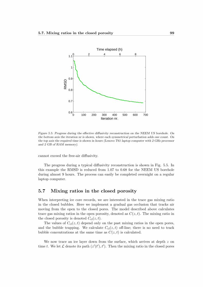
5.7. Mixing ratios in the closed porosity 99

0 100 200 300 400 500 600 7000.6

0.7

0.8

0.9

1

1.1

RM

SD

Iteration nr.

0 2 4 6 8

Time elapsed (h)

Figure 5.5: Progress during the effective diffusivity reconstruction on the NEEM US borehole. Onthe bottom axis the iteration nr is shown, where each symmetrical perturbation adds one count. Onthe top axis the required time is shown in hours (Lenovo T61 laptop computer with 2 GHz processorand 2 GB of RAM memory).

cannot exceed the free-air diffusivity.

The progress during a typical diffusivity reconstruction is shown in Fig. 5.5. Inthis example the RMSD is reduced from 1.07 to 0.68 for the NEEM US boreholeduring almost 9 hours. The process can easily be completed overnight on a regularlaptop computer.

5.7 Mixing ratios in the closed porosity

When interpreting ice core records, we are interested in the trace gas mixing ratioin the closed bubbles. Here we implement a gradual gas occlusion that tracks airmoving from the open to the closed pores. The model described above calculatestrace gas mixing ratios in the open porosity, denoted as C(z, t). The mixing ratio inthe closed porosity is denoted Ccl(z, t).

The values of Ccl(z, t) depend only on the past mixing ratios in the open pores,and the bubble trapping. We calculate Ccl(z, t) off-line; there is no need to trackbubble concentrations at the same time as C(z, t) is calculated.

We now trace an ice layer down from the surface, which arrives at depth z ontime t. We let L denote its path (z′(t′), t′). Then the mixing ratio in the closed pores

100 Chapter 5. The CIC firn air model

50 100 150

0

0.01

0.02

0.03

0.04

Age (yr)

Age

dis

trib

utio

n G

(yr

−1 )

ClosedOpen

0 100 200 300 400 500

0

2

4

6

8

10

12

14

16

x 10−3

Age (yr)

Age

dis

trib

utio

n G

(yr

−1 )

ClosedOpen

a) b)

Figure 5.6: Calculated CH4 age distributions at the bottom of the firn column in the open andclosed porosities at a) NEEM (z = 79 m) and b) South Pole (z = 123 m). Note the difference inscale on the horizontal and vertical axes.

is given by

Ccl(z, t) =1

φcl

∫LC(L)dφcl

=1

φcl

∫ t

t−ηC(z′(t′), t′)

1

wice

dφcl

dz′dt′ (5.33)

where η is the time it takes the ice parcel to sink from 0 to z, given by

η =1

Aρice

∫ z

0ρdz′ (5.34)

The model first calculates the open pore mixing ratios C(z, t), which are stored in amatrix Cop with a typical resolution of ∆z = 0.5 m and ∆t = 0.01 yr. We find theterm C(z′(t′), t′) in Eq. 5.33 by linear interpolation along z′ of the elements of thematrix Cop.

In Fig. 5.6 we show calculated CH4 age distributions at the bottom of the firncolumn at the NEEM and South Pole sites. In Table. 5.1 we give the characteristicsof the age distributions, using two commonly used metrics. The first one is the meanage Γ(z), which is the first moment of the distribution:

Γ(z) =

∫ ∞0

t ·G(z, t) dt (5.35)

5.8. Summary and conclusions 101

Table 5.1: Mean age Γ and spectral width ∆ for CH4 at NEEM (z = 79 m) and South Pole (z = 123m). All values are in years.

Open pores Closed pores

NEEM Γ 72.2 73.6NEEM ∆ 9.4 9.5

South Pole Γ 100.9 149.0South Pole ∆ 21.8 54.6

The second is the spectral width ∆(z), which is the second moment of the distribution(Trudinger et al., 2002):

∆2(z) =1

2

∫ ∞0

(t− Γ)2 ·G(z, t) dt (5.36)

The trapping process has two effects. First, the air in the closed pores is olderthan the air in the open pores, as can be seen from the mean age Γ. This is causedby a tail of older air that is already trapped in the DZ. Second, the trapping processcauses some additional smoothing, which is shown by an increased distribution width∆.

It is also clear that the effects of trapping are almost negligible at a high accu-mulation site such as NEEM. The low accumulation rate and long firn column atSouth Pole make the effects of the bubble trapping clearly visible. Another impor-tant difference between the two sites is the length of the LIZ, or non-diffusive zone.At NEEM the LIZ is very long, with only an estimated ∼5 % of the bubbles trappedabove the lock-in depth. At South Pole the LIZ is very narrow, and an estimated∼20 % is trapped above the lock-in depth (using the Goujon et al. (2003) parame-terization in both cases). In particular bubble trapping in the DZ leads to additionalbroadening of the age distribution. Within the LIZ, bubble trapping does not leadto a significant broadening because the air is advected downwards at approximatelythe same velocity as the ice.

5.8 Summary and conclusions

In this chapter we introduced the CIC 1-D firn air transport model:

• Using the principle of mass conservation, we derived expressions for the airvelocity in the open porosity and the bubble trapping rate.

• Based on two simple assumptions, we derived an expression for the pressur-ization of closed bubbles due to firn compaction. We tested the equationsfor NEEM and South Pole, and found they predicted the total air contentaccurately within 3%.

102 Chapter 5. The CIC firn air model

• We described the total flux of a tracer in the open porosity.

• We showed how the second order PDE describing the combined effects of diffu-sion, advection and radioactive decay was implemented numerically using theCrank-Nicolson method.

• We presented a new way to reconstruct the effective diffusivity profile withdepth.

• We showed how mixing ratios in the closed porosity can be calculated, andshowed how the trapping process broadens the age distribution. We found theadditional broadening due to trapping to be negligible at NEEM, because ofits high accumulation and long lock-in zone. At South pole there is significantbroadening due to the lower accumulation rate and the short lock-in zone.

5.9 References

Colbeck, S. C. (1989). Air movement in snow due to windpumping. J. Glaciol., 35(120):209–213.Goujon, C., Barnola, J. M., and Ritz, C. (2003). Modeling the densification of polar firn including

heat diffusion: Application to close-off characteristics and gas isotopic fractionation for antarcticaand greenland sites. J. Geophys. Res.-Atm, 108(D24):18.

Huber, C., Beyerle, U., Leuenberger, M., Schwander, J., Kipfer, R., Spahni, R., Severinghaus, J. P.,and Weiler, K. (2006). Evidence for molecular size dependent gas fractionation in firn air derivedfrom noble gases, oxygen, and nitrogen measurements. Earth Planet Sc. Lett., 243(1-2):61–73.

Kawamura, K., Severinghaus, J. P., Ishidoya, S., Sugawara, S., Hashida, G., Motoyama, H., Fujii,Y., Aoki, S., and Nakazawa, T. (2006). Convective mixing of air in firn at four polar sites. EarthPlanet Sc. Lett., 244(3-4):672–682.

Martinerie, P., Raynaud, D., Etheridge, D. M., Barnola, J. M., and Mazaudier, D. (1992). Physicaland climatic parameters which influence the air content in polar ice. Earth Planet Sc. Lett.,112(1-4):1–13.

Rommelaere, V., Arnaud, L., and Barnola, J. M. (1997). Reconstructing recent atmospheric tracegas concentrations from polar firn and bubbly ice data by inverse methods. J. Geophys. Res.-Atm,102(D25):30069–30083.

Schwander, J. (1989). The transformation of snow to ice and the occlusion of gases. In Oescher,H. and Langway, C., editors, The Environmental record in glaciers and ice sheets, pages 53–67.John Wiley, New York.

Schwander, J., Barnola, J. M., Andrie, C., Leuenberger, M., Ludin, A., Raynaud, D., and Stauffer,B. (1993). The age of the air in the firn and the ice at summit, greenland. J. Geophys. Res.-Atm,98(D2):2831–2838.

Severinghaus, J. P. and Battle, M. O. (2006). Fractionation of gases in polar lee during bubbleclose-off: New constraints from firn air ne, kr and xe observations. Earth Planet Sc. Lett., 244(1-2):474–500.

Severinghaus, J. P., Grachev, A., and Battle, M. (2001). Thermal fractionation of air in polar firnby seasonal temperature gradients. Geochem. Geophy. Geosy., 2.

Sowers, T., Bender, M., Raynaud, D., and Korotkevich, Y. S. (1992). Delta-n-15 of n2 in airtrapped in polar ice - a tracer of gas-transport in the firn and a possible constraint on ice age-gasage-differences. J. Geophys. Res.-Atm, 97(D14):15683–15697.

Sugawara, S., Kawamura, K., Aoki, S., Nakazawa, T., and Hashida, G. (2003). Reconstruction ofpast variations of delta c-13 in atmospheric co2 from its vertical distribution observed in the firnat dome fuji, antarctica. Tellus B, 55(2):159–169.

5.9. References 103

Trudinger, C. M., Enting, I. G., Etheridge, D. M., Francey, R. J., Levchenko, V. A., Steele, L. P.,Raynaud, D., and Arnaud, L. (1997). Modeling air movement and bubble trapping in firn. J.Geophys. Res.-Atm, 102(D6):6747–6763.

Trudinger, C. M., Etheridge, D. M., Rayner, P. J., Enting, I. G., Sturrock, G. A., and Langenfelds,R. L. (2002). Reconstructing atmospheric histories from measurements of air composition in firn.J. Geophys. Res.-Atm, 107(D24):13.

104 Chapter 5. The CIC firn air model

6In situ cosmogenic radiocarbon production and 2-D ice

flow line modeling for an Antarctic blue ice area

C. Buizert, V. V. Petrenko, J. L Kavanaugh, K. M. Cuffey,N. A. Lifton, E. J. Brook and J. P. Severinghaus1

6.1 Introduction

Old ice can not only be obtained from deep ice cores, but also at ice margins andAntarctic blue ice areas (BIAs) where it is being re-exposed by ablation (Reeh et al.,2002; Bintanja, 1999). For paleoclimate studies this provides an interesting alterna-tive to ice coring, as sample retrieval is less challenging both from a technologicaland a logistical point of view. Ice can be sampled from near the surface, mak-ing the method especially well suited for experiments that require large ice samples(Petrenko et al., 2009). Dating of ice parcels is the principal problem when usingablation sites for climatic reconstruction (Sinisalo and Moore, 2010, and referencestherein). Several methods have been used, including radiometric dating of tephralayers (e.g. Dunbar et al., 2008), flow line modeling (Azuma et al., 1985; Grinstedet al., 2003; Moore et al., 2006), stratigraphical matching of gas and stable waterisotope measurements to well-dated ice core records (e.g. Reeh et al., 2002; Petrenkoet al., 2006; Aciego et al., 2007; Schaefer et al., 2009), and radiocarbon dating ofmicro-particles (Jenk et al., 2007). Early on it was realized that radiocarbon (14C)dating of the CO2 present in the air bubbles trapped in polar ice can potentiallybe used as an absolute dating method for ice cores and BIA samples (Fireman andNorris, 1982; Andree et al., 1984). However, interpretation of radiocarbon data iscomplicated by cosmogenic in situ production of 14C from oxygen atoms found inice (Lal et al., 1990). When this effect is corrected for, the air bubbles containedin the ice can be dated with an accuracy of a few thousands of years (Van de Wal

1This chapter has been submitted to the Journal of Geophysical Research – Earth Surface.

105

106 Chapter 6. In situ radiocarbon and 2-D ice flow at a BIA

et al., 1994; Van Roijen et al., 1995; Van Der Kemp et al., 2002; De Jong et al., 2004;Van de Wal et al., 2007).

Apart from dating applications, there are other reasons for studying radiocarbonin ice. First, surface 14C concentrations reflect ablation (or accumulation) rates atthe site under study. At low ablation rate sites the ice parcels move slowly throughthe top ∼5 m (where cosmogenic irradiation is strongest), leading to high surfaceactivities as the in situ produced 14C accumulates over time. And vice versa, whereablation rates are high, activities will be low. By this principle, measurements of14C have been used to estimate BIA ablation rates (e.g., Lal et al., 1990; Van Roijenet al., 1995; Van der Borg et al., 2001). It has also been suggested that 14C in icecore samples can be used to infer past changes in accumulation rate (Lal et al., 1990,2000).

Second, at well-dated ablation sites paleoclimate information can be obtainedfrom radiocarbon measurements. Fossil carbon sources are depleted in 14C, and inthis way measuring 14C activities of carbon-containing gas species can teach us aboutthe fossil contribution to their past atmospheric variations. In particular, the 14Cvariations in methane (CH4) over the last glacial termination contain informationon how much the destabilization of 14C-depleted methane hydrates contributed tothe observed CH4 increases (Petrenko et al., 2008, 2009).

Here we study 14C production at the Taylor Glacier BIA, Antarctica, where icewith ages between approximately 11.5 and 65 kyr is being exposed (Aciego et al.,2007; Kavanaugh et al., 2009b). Taylor Glacier is an outlet glacier of the East Antarc-tic Ice Sheet which originates at Taylor Dome, and terminates in the McMurdo DryValleys (Figure 6.1). Ablation is dominated by sublimation (Bliss et al., 2011); ab-lation rates are around 0.1-0.3 m yr−1 (Kavanaugh et al., 2009a), which is typical ofAntarctic BIAs (Bintanja, 1999). The ice stratigraphy along the center flow line canbe dated by matching trace gas mixing ratios and gas stable isotope measurementsto ice core records, and matching of water stable isotopes to the Taylor Dome record(Steig et al., 2000). The large (∼1000 kg) ice samples required for high precision 14Cmeasurements of trace gas species such as CH4 and CO can be obtained from nearthe glacier surface (Petrenko et al., 2008).

Because measurable amounts of cosmogenic 14C are produced down to a depthof ∼ 200 m, the exposure history of ablating ice parcels is a function of their flowpath in the glacier. The aim of this study is to combine 2-D flow line modelingwith up-to-date cosmogenic exposure theory to obtain a best estimate for the 14Cactivity of ablating Taylor Glacier ice. We present two new ways to parameterizevertical strain rates with depth, and we evaluate which method provides the betterdescription for Taylor Glacier. The model allows us to assess the influence of glaciervalley topography and solar modulation of cosmic ray intensity on the in situ 14Cproduction; both of which have been neglected in studies so far.

6.2. Cosmogenic production of 14C in ice 107

T a y l o r

G l a c

i e r

F e r r a r G

l a c i e r

Beac

on V

alle

y

Aren

a Va

lley

CRCIF

K u k r i H i l l s

Pearse Valley

SB

DepotNunatak

Turnabout Valley

Taylor-Ferrar Confluence

A s g a r d R a n g e

PS

WG

Friis Hills

LB

’ E00°261’ E00°161 ’03°261’0 E3°161160°30’ E160°00’ E

77°5

0’ S

RM

77°4

5’ S

77

°40’

S

10 km

Cass

idy

Gla

cier

Figure 6.1: The Taylor Glacier with surroundings. Abbreviations are: Round Mountain (RM),Simmons Basin (SB), Pandora Spire (PS), the Cavendish Ice Falls (CIF), Cavendish Rocks (CR),Windy Gully (WG), and Lake Bonney (LB).

The modeling results presented here will furthermore be used for interpretationof future 14C measurements. During a 2010/2011 Austral summer field campaign,samples for radiocarbon analyses were taken at Taylor Glacier with the purposeof constraining in situ production rates better. We will show that at the samplinglocation the influence of ice flow strain rates on 14C activities is minimal, greatly sim-plifying data interpretation. More importantly, this work will serve as a frameworkfor correcting 14C of methane (14CH4) measurement over the last glacial terminationfor the effects of in situ production, with the purpose of reconstructing of the truepaleo-atmospheric signal.

6.2 Cosmogenic production of 14C in ice

Cosmic rays consist largely of charged subatomic particles originating from outsidethe Earth’s magnetosphere. Upon entering the upper atmosphere, particles of suf-ficient energy cause nuclear disintegrations, from which a shower, or cascade, ofsecondary cosmic ray particles is produced. On interacting with the materials ofEarth’s surface, these secondary cosmic rays are capable of producing a wide varietyof terrestrial cosmogenic nuclei (TCN); see Gosse and Phillips (2001) and referencestherein for an overview of TCN exposure theory. In ice, 14C is produced cosmogeni-

108 Chapter 6. In situ radiocarbon and 2-D ice flow at a BIA

cally, primarily through neutron spallation of oxygen atoms (Lal et al., 1990). Afterproduction, the 14C atoms are predominantly oxidized to form either 14CO2 or 14CO.The reported fraction of 14CO out of the total in situ 14C ranges from 0.20-0.57 (Lalet al., 1990; Van Roijen et al., 1995; Lal et al., 2000; Van Der Kemp et al., 2002;De Jong et al., 2004). A recent study, however, suggests 14CH4 is formed in smallamounts as well (Petrenko et al., 2009).

Ice found in BIAs has experienced two intervals of exposure: one in the accumu-lation zone and one during ablation. Interpretation of the ablation signal is morestraightforward because all the cosmogenic 14C is retained. In the accumulationzone, the presence of a porous firn layer complicates interpretation. In their concep-tual model of 14C retention in the firn, Van de Wal et al. (2007) introduce a degassingrate at which 14C is released from the ice matrix (where it is produced), into theopen pore space. From there, the produced 14C is lost to the overlying atmospherethrough the action of diffusion and wind pumping. Some authors have argued thatthe degree to which 14C is retained in the firn may depend on the accumulation rate(Lal et al., 2001; De Jong et al., 2004). Their arguments are based on the observationthat the high accumulation Greenland GISP2 ice core (0.25 m yr−1 ice equivalent)showed high retention of in situ 14C (Lal et al., 2000), while low accumulation sitessuch as Dome Concordia (0.03 m yr−1), Vostok (0.02 m yr−1) and Taylor Dome (0.06m yr−1) show low or no retention (Lal et al., 2001; De Jong et al., 2004). However,this hypothesis is contradicted by reported observations of high retention at a lowaccumulation site (Jull et al., 1994), as well as low retention at high accumulationsites (Smith et al., 2000, Petrenko et al., in preparation). It has also been proposedthat the method used to extract gas from ice samples can influence the results (Smithet al., 2000; Van der Borg et al., 2001). Dry extraction methods, such as milling andgrating (Van de Wal et al., 1994; Smith et al., 2000), will liberate gas molecules inair bubbles, but might not extract all the gas molecules dissolved in the ice. Sincein situ cosmogenic 14C is produced in the ice matrix rather than in the bubbles, dryextraction methods may underestimate cosmogenic 14C content. Melt extractionwith added phosphoric acid (Lal et al., 1990) will extract all gas molecules, howeveradditional CO2 will be produced from any (bi)carbonates present in the ice. Withthis technique CO2 and CO may also be produced from organics in the ice. Giventhe results published to date, it is unclear how much of the 14C that is produced inthe accumulation zone is actually retained, if any. We focus our attention on 14Cproduction in the ablation zone. For ice older than ∼ 50 kyr, essentially all of theaccumulation-zone cosmogenic 14C will have decayed, and only the ablation-zonecomponent is of importance.

We will consider four different mechanisms of in situ cosmogenic 14C productionin ice. Three of these involve nuclear reactions with oxygen; the fourth involvesthe capture of thermal neutrons by the nitrogen present in the air bubbles found inglacial ice.

6.2. Cosmogenic production of 14C in ice 109

102

103

104

10−2

10−1

100

101

102

Depth Z (g cm−2)

P(z

) (g

−1 yr

−1 )

SpallationMuon capt.Fast muonTotal

100

101

102

Depth z (m)

0 500 1000 1500 20000

0.5

1

1.5

2

2.5x 10

4

Altitude (m)

Q (

cm−

2 yr−

1 )

SpallationMuon capt.Fast muon

A

B

Figure 6.2: (A) In situ 14C production rates with glacier depth using equation (6.1) and the valueslisted in Table 6.1. The glacier surface is taken at sea level. The black dashed line represents thesum of the individual mechanisms. (B) Altitude dependence of the production using the Lifton et al.(2005) model. The colors represent the three mechanisms, the vertical axis shows the integratedproduction Qi =

∫∞0Pi(z)dz.

6.2.1 Spallogenic and muogenic production

We first consider neutron spallation reactions (Lal et al., 1990, 2000), negative muoncapture (Van der Borg et al., 2001; Van Der Kemp et al., 2002; Heisinger et al.,2002a), and fast muon reactions (Heisinger et al., 2002b; Nesterenok and Naidenov,2009). The neutron and muon fluxes incident on the glacier surface are attenuatedin the ice, giving a production P (z) that falls off with depth following

Pi(z) = P 0i e−Z/Λi = P 0

i e−ρz/Λi (6.1)

where P 0i is the surface production rate, Z the overburden in g cm−2, z the depth

in cm, Λi the absorption mean free path in g cm−2, and ρ the density of the medium(for ice we use ρ = 0.92 g cm−3). Following Heisinger et al. (2002a), the subscript

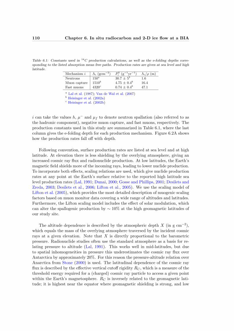
110 Chapter 6. In situ radiocarbon and 2-D ice flow at a BIA

Table 6.1: Constants used in 14C production calculations, as well as the e-folding depths corre-sponding to the listed absorption mean free paths. Production rates are given at sea level and highlatitude.

Mechanism i Λi (gcm−2) P 0i (g−1yr−1) Λi/ρ (m)

Neutrons 150a 30.7 ± 5b 1.6

Muon capture 1510b 4.75 ± 0.4b 16.4

Fast muons 4320c 0.74 ± 0.4b 47.1

a Lal et al. (1987); Van de Wal et al. (2007)b Heisinger et al. (2002a)c Heisinger et al. (2002b)

i can take the values h, µ− and µf to denote neutron spallation (also referred to asthe hadronic component), negative muon capture, and fast muons, respectively. Theproduction constants used in this study are summarized in Table 6.1, where the lastcolumn gives the e-folding depth for each production mechanism. Figure 6.2A showshow the production rates fall off with depth.

Following convention, surface production rates are listed at sea level and at highlatitude. At elevation there is less shielding by the overlying atmosphere, giving anincreased cosmic ray flux and radionuclide production. At low latitudes, the Earth’smagnetic field shields more of the incoming rays, leading to lower nuclide production.To incorporate both effects, scaling relations are used, which give nuclide productionrates at any point at the Earth’s surface relative to the reported high latitude sealevel production rates (Lal, 1991; Dunai, 2000; Gosse and Phillips, 2001; Desilets andZreda, 2003; Desilets et al., 2006; Lifton et al., 2005). We use the scaling model ofLifton et al. (2005), which provides the most detailed description of muogenic scalingfactors based on muon monitor data covering a wide range of altitudes and latitudes.Furthermore, the Lifton scaling model includes the effect of solar modulation, whichcan alter the spallogenic production by ∼ 10% at the high geomagnetic latitudes ofour study site.

The altitude dependence is described by the atmospheric depth X (in g cm−2),which equals the mass of the overlying atmosphere traversed by the incident cosmicrays at a given elevation. Note that X is directly proportional to the barometricpressure. Radionuclide studies often use the standard atmosphere as a basis for re-lating pressure to altitude (Lal, 1991). This works well in mid-latitudes, but dueto spatial inhomogeneities in pressure this underestimates the cosmic ray flux overAntarctica by approximately 20%. For this reason the pressure-altitude relation overAnarctica from Stone (2000) is used. The latitudinal dependence of the cosmic rayflux is described by the effective vertical cutoff rigidity RC , which is a measure of thethreshold energy required for a (charged) cosmic ray particle to access a given pointwithin the Earth’s magnetosphere. RC is inversely related to the geomagnetic lati-tude; it is highest near the equator where geomagnetic shielding is strong, and low

6.2. Cosmogenic production of 14C in ice 111

at the poles where the threshold energy is low and essentially all cosmic rays of in-terest to cosmogenic nuclide production are admitted. The scaling model is latitudeinvariant at geomagnetic latitudes greater than approximately ∼ 60◦ S, equivalent toRC ≤ 1.9 (Lifton et al., 2005). Taylor glacier falls within this latitude range. Figure6.2B shows how the integrated ice column production Qi =

∫∞0 Pi(z)dz changes with

altitude. The integrated production Qi scales linearly with the surface productionP 0i , but is more informative since it shows the total amount of in situ 14C that will

be present in an ablating ice parcel. It is clear that the neutron flux is attentuatedmuch more strongly by the atmosphere, giving a more pronounced altitude depen-dence.

6.2.2 Thermal neutron capture

Glacial ice contains a finite amount of trapped air, typically about 0.1 mL g−1 atstandard temperature and pressure (STP). The final mechanism of 14C productionwe consider is absorption of thermal neutrons by the nitrogen present in gas bubbles,following the 14N(n,p)14C nuclear reaction pathway. This is the dominant mecha-nism for radiocarbon production in the atmosphere. To the best of our knowledge,this mechanism has been ignored in studies of radiocarbon production in ice to date.However, because of the large capture cross-section of nitrogen (σth,N = 1.9× 10−24

cm2), a thermal neutron contribution cannot be excluded a priori.

Low-energy neutrons, such as thermal neutrons, originate from fast (spallogenic)neutrons whose energy has been moderated through interaction with matter (Gosseand Phillips, 2001). On slowing down they first pass through the epithermal energyrange (0.5eV < En < 1 keV, with En the neutron energy). By this time, the particletrajectories have been fully randomized, and the epithermal neutron flux is diffusivein nature. While a fraction of the epithermal neutrons will be captured by surround-ing nuclei, the remainder is moderated further and reaches the thermal energy range(0 < En < 0.5 eV), where neutron energy is on the order of the thermal vibrationsof their surroundings. At these energies they can no longer lose their energy bymomentum transfer to incident nuclei, and the only sink mechanisms to the thermalneutron flux are capture and free neutron decay.

To calculate both the epithermal and thermal neutron fluxes near the ice-atmosphereinterface, we use a model by Phillips et al. (2001). Table 6.2 lists the low-energytransport parameters used here, where for each element k we specified its mass A,average log decrement of energy loss per collision ξ, epithermal neutron scatteringcross-section σsc, thermal neutron capture cross-section σth and the dilute resonanceintegral for absorption of epithermal neutrons Ia. We also specified the estimatedconcentrations in atoms per gram of the different elements for both ice and atmo-sphere (Nice and Natm, respectively). We first verified our low-energy neutron modelby comparing our calculated fluxes to measured fluxes in a block of concrete at Los

112 Chapter 6. In situ radiocarbon and 2-D ice flow at a BIA

0

5000

10000

15000N

eutr

on fl

ux (

cm−

2 yr−

1 )

Epithermal FluxThermal Flux

−250 0 0.5 1 1.5

Depth z (m)

−50 0 50 100 1500

0.05

0.1

0.15

0.2

Depth Z (g cm−2 )

P(Z

) (g

−1 y

r−1 )

Asymptote P

th(Z)

A

B

Figure 6.3: (A) Modeled thermal and epithermal neutron fluxes at the atmosphere-ice interfaceat high latitude (RC = 0) and sea level. The ice surface is placed at Z = 0; for Z < 0 we haveatmosphere, for Z ≥ 0 ice. (B) Production rate of 14C through the 14N(n,p)14C nuclear reactiongiven the calculated neutron fluxes, together with the asymptote given by equation (6.4).

Alamos National Laboratory, USA (Liu et al., 1994). The model reproduces theobservations within 10%, giving us confidence that, at the very least, the modelwill calcluate the fluxes to the correct order of magnitude. Figure 6.3A shows thecalculated epithermal and thermal fluxes (Φeth and Φth, respectively) for an ice-atmosphere interface at sea level. We see that the epithermal flux in the ice isstrongly reduced. This is due to the presence of hydrogen as the most abundantelement, which is a very effective moderator of epithermal neutrons (Table 6.2). Theprobability that epithermal neutrons are absorbed in the ice is given by

p(Eeth) = 1− exp

(−∑

k Ia,kNice,k∑k σsc,kNice,k

)< 1× 10−5 (6.2)

This indicates that effectively all epithermal neutrons are further moderated into thethermal energy range, rather than absorbed. Accordingly, we see a large increase inthe thermal neutron flux over the atmosphere-ice interface.

From the calculated flux we can derive the production of 14C by thermal neutronsas

6.3. Taylor Glacier 2-D flow line modeling 113

Table 6.2: Low-energy neutron transport parameters for the elements under consideration. Valuesare taken from Phillips et al. (2001) unless indicated differently.

k A ξ σsc σth Ia Nice Natm

(g mol−1) (unitless) (10−24 cm2) (10−24 cm2) (10−24 cm2) (1020 g−1) (1020 g−1)H 1 1 20.5 0.33 0 667 0N 14 0.14 11.5a 1.9b 0.034c 0.0456 325O 16 0.12 3.76 0.0002 0.0004 334 87.1Ar 39.9 0.049 0.68a 0.675a 0.41c 0.0027 1.94

a Sears (1992)b Wagemans et al. (2000)c Mughabghab et al. (1992)

Pth(Z) = σth,NNice,NΦth(Z) (6.3)

This is shown in Figure 6.3B together with the curve

PASth (Z) = σth,NNice,NΦ∗th,icee

−Z/Λh (6.4)

towards which Pth(Z) approaches asymptotically as Z → ∞. The value of Φ∗th,ice

is given by equation (21) in Phillips et al. (2001). From equation (6.4) it is clearthat in first approximation the thermal neutron production has the same depthdependence as the production by neutron spallation (equation (6.1)); however, thesurface production rate (and thereby the integrated column production), is morethan 2 orders of magnitude smaller. We shall therefore neglect 14C production bythermal neutrons in the remainder of this work. Since all thermal neutrons areultimately captured by nuclei of the host material, one might wonder why the 14Cproduction rate is so small. On comparing the values in Table 6.2 it is clear thathydrogen absorbs the vast majority of thermal neutrons by virtue of its abundanceand relatively large capture cross-section.

6.3 Taylor Glacier 2-D flow line modeling

6.3.1 Data input to the ice flow model

The 2-D ice flow line modeling presented here is based on a recent detailed studyof the dynamics and mass balance of Taylor Glacier (Kavanaugh et al., 2009a; Ka-vanaugh and Cuffey, 2009; Kavanaugh et al., 2009b). From these studies we usethe surface and basal digital elevation models; surface velocities obtained from bothsatellite radar interferometry (InSAR) and Global Positioning System (GPS) mea-surements of the displacement of a network of survey poles; ice-surface ablation rates;and modeled horizontal velocity profiles with depth.

Figure 6.4 shows the outline of the glacier, with the color scale depicting themagnitude of the surface velocity in m yr−1 obtained through remote sensing (Ka-vanaugh et al., 2009b). The red line indicates the flow line used in this study, along

114 Chapter 6. In situ radiocarbon and 2-D ice flow at a BIA

535 540 545 550 555 560 565 570 575

1355

1360

1365

1370

1375

1380

UTM Easting (km)

UT

M N

orth

ing

(km

)

0510

15

20

2530

35

40

45

50

55

0

2

4

6

8

10

12

14

16

18

20

Figure 6.4: Color plot of glacier surface velocity in m yr−1 from InSAR (Kavanaugh et al., 2009b).Regions with missing data show up as light patches; here high surface deformation due to strainrates precludes phase unwrapping. White dots indicate survey poles used in this study, which are asubset of the stake network of Kavanaugh et al. (2009b), selected for their proximity to the center-line flow path. Ablation rate measurements as well as GPS velocity measurements are available forthese poles. The red line with distance markers in km indicates the center flow line used in thisstudy, the black line shows the glacier edge. The main 14C sampling site of the 2010/2011 Australsummer field campaign (77.762◦ S, 161.720◦ E, or x = 14.05 km) is indicated with a yellow diamond.

which we shall calculate the exposure history of ablating ice parcels. The marks inred give the distance from the glacier terminus in km along the flow line. We let xbe the flow-parallel coordinate with the origin at the terminus, y be perpendicularto the flow and z be the depth coordinate with z = 0 at the glacier surface. The flowline is constructed in two steps. The first part from 0 < x ≤ 40.5 km follows the sam-pling transect of a 2009-2010 field campaign, the aim of which was to accurately datethe ablating ice (D. Baggenstos, in preparation). For x > 40.5 km we inverted thesurface velocity field and traced back an imaginary ice parcel. The flow line crossestwo narrow regions of missing data around x = 53 km; in these locations we adjustedthe path by eye to obtain a smooth transition between the trajectories on both sides.

The ablation rate measurements are described by Kavanaugh et al. (2009a). Weselected poles along the center flow line as shown in Figure 6.4. The poles wereplanted during the 2002/2003 Austral summer field season, and measured duringthe 2003/2004 season. The majority of poles relevant for this study were remeasuredin the 2006/2007 season. We include additional data for a total of 17 poles thatwere remeasured during the 2009/2010 and 2010/2011 field seasons. Consequently

6.3. Taylor Glacier 2-D flow line modeling 115

we have 1- and 4-year ablation rate estimates for the majority of the poles, and a7- or 8-year estimate for 17 of the poles. The 1- and 4-year ablation rate estimatesdiffer significantly, with the former being 4.7 cm yr−1 more rapid averaged over theselected poles (Kavanaugh et al., 2009a). The 4-year estimates agree well with theand 7- and 8-year averages. For each pole we take the longest available measure-ment period as a best estimate. For 7 poles (all at x > 50 km) this period equalsone year; their ablation estimate is adjusted by subtracting 4.7 cm yr−1. The sin-gle year ablation offset from the long term average gives an estimate of the year toyear variability; as an ablation rate uncertainty estimate we use 4.7 cm yr−1 dividedby√N , where N is the period in years (N = 1, 4, 7, 8). Pole positions were pro-

jected perpendicularly onto the flow line; poles with their x coordinate less than 200m apart were averaged. Between stakes we used linear interpolation of both abla-tion rates and uncertainty estimates. The peak near x = 30 km is caused by strongkatabatic winds coming down Windy Gully (Figure 6.1; see Kavanaugh et al., 2009a).

6.3.2 Calculating vertical ice velocities relative to the surface

To trace the trajectories of ice parcels downwards back into the glacier, we need tocalculate flow velocities in the x, z-plane. Let u, v, w be the velocity componentsalong x, y, z; u = (u, v) the horizontal velocity vector, us = (us, vs) the horizontalvelocity vector at the glacier surface, and H the total ice thickness. The componentw is the vertical velocity relative to the glacier surface. We write the horizontalvelocity as (Azuma et al., 1985; Grinsted et al., 2003; Kavanaugh and Cuffey, 2009):

u(z) = f(z)us

v(z) = f(z)vs = 0 (6.5)

where f(z) is a scaling function which equals unity at the surface f(0) = 1. Ka-vanaugh and Cuffey (2009) conclude that Taylor Glacier is frozen to the bed; forthis reason we include no basal sliding, and f goes to zero at bedrock f(H) = 0.We use the numerically solved scaling functions by Kavanaugh and Cuffey (2009)at six points along the flow line, and use linearly interpolated profiles in between.The profiles are accurate since they are based on the actual stresses and estimatedtemperature profiles in Taylor Glacier.

The vertical velocity at the surface equals the ablation rate ws = a. At finitedepth w(z) is given by

w(z) = a+

∫ z

0εzz(z

′)dz′ (6.6)

where εzz is the vertical strain rate εzz = ∂w/∂z. We will compare two methods toestimate εzz.

116 Chapter 6. In situ radiocarbon and 2-D ice flow at a BIA

Estimating εzz using mass conservation in the ice column

Kavanaugh et al. (2009a) have estimated that within the accuracy of their method,Taylor Glacier is in steady state. Under this assumption (∂H/∂t = 0), mass conser-vation in the ice column can be written as (Cuffey and Paterson, 2010)

a+H(∇ · u) + u · (∇H) = 0 (6.7)

where u is the depth-averaged horizontal velocity. We introduce the commonly usedassumption that the horizontal strain rates scale the same way with depth as thehorizontal velocity (Grinsted et al., 2003; Kavanaugh and Cuffey, 2009)

εxx =∂u

∂x= f(z)

∂us

∂x

εyy =∂v

∂y= f(z)

∂vs

∂y(6.8)

This is not always a good assumption near the bed, but works well for the near-surface flow that is relevant to cosmogenic production estimation. Using the factthat on the center flow line the transverse velocity vs = 0 we can rewrite equation(6.7) as

a+Hf

(∂us

∂x+∂vs

∂y

)+ fus

∂H

∂x= 0 (6.9)

where f is the column average f = 1H

∫ H0 f(z)dz. Equation (6.9) assumes that

∂f/∂x can be neglected. Using the incompressibility of ice we can solve for thevertical strain rate

εzz(z) = −f(z)

H

(a

f+ us

∂H

∂x

)(6.10)

Note that this approach is similar to that developed by Grinsted et al. (2003); themain difference is the inclusion of the us∂H/∂x term on the right hand side of equa-tion (6.10), which is neglected in the cited study. For Taylor Glacier we cannotneglect this term, as there are large longitudinal variations in glacier thickness. Tocalculate vertical velocities with this approach, we use measurements of: (1) ablationrates, (2) horizontal velocity field (us, vs), and (3) ice thickness H along the flow line.

This method does not ensure that w(H) = 0. After calculating w(z) usingequation (6.6) and 6.9 we have forced the ice near the base (0.8H < z < H) totransition smoothly towards flow parallel to the bed, or w(z) = ∂H/∂x · u(z). Notethat because the 14C production happens in the upper part of the column only, thiswill not significantly influence our results.

6.3. Taylor Glacier 2-D flow line modeling 117

0 10 20 30 400

0.1

0.2

0.3

0.4

Distance from terminus (km)

Abl

atio

n ra

te (

m/y

r)

−6 −4 −2 0 2 4

x 10−3

−6

−4

−2

0

2

4x 10

−3

GPS pole strain rate

InS

AR

str

ain

rate

Slope = 1.1 R2 = 0.68

[du / dx]s

[dv / dy]s

0 10 20 30 40

0

500

1000

1500

Distance from terminus x (km)

Alti

tude

(m

a.s

.l.)

A

B

C

Figure 6.5: (A) Ablation rates from stake measurements (Kavanaugh et al., 2009a, black dots witherror bars) together with the interpolated best estimate (blue line) and uncertainty estimate (lightblue shading). The longitudinal ablation rate profile is further analyzed by Bliss et al. (2011).Details on the uncertainty estimate are given in the text. (B) Comparison of surface strain ratesestimates obtained from the GPS stake network (Kavanaugh et al., 2009b, horizontal axis) andthrough remote sensing (vertical axis). Outlier on left rejected in the slope fitting. (C) Uncertaintyin flow line reconstruction, details given in the text. The arrow shows the location of the 14Csampling site of the 2010/2011 field campaign.

118 Chapter 6. In situ radiocarbon and 2-D ice flow at a BIA

Estimating εzz from measured surface strain rates

As an alternative approach we calculate vertical strain from estimates of horizontalstrain rates derived from InSAR and GPS surface flow velocities. Let εMxx,s and εMyy,sbe the longitudinal and transverse surface strain rate estimates from measurementsof us. Using assumption 6.8 and the incompressibility of ice we obtain

εzz(z) = −(εMxx,s + εMyy,s

)f(z) (6.11)

The reliability of this approach depends on the accuracy of the surface strain rate es-timates. Figure 6.5B shows a comparison between strain rate estimates based on theInSAR and GPS data. We see that the slope of the correlation deviates significantlyfrom unity; there is one clear outlier in the transverse strain rate εyy; there is muchscatter in the data (R2 = 0.68 when ignoring the outlier); and for ∼20% of the pointsthe sign is reversed. In equation (6.11) the horizontal strain rates are added up. Bydoing so the potential for error is increased further, as their uncertainties also add up.

When calculating ice flow trajectories based on this second approach, we find thatthey fail to follow bedrock undulations as required. Furthermore, mass conservationis violated as ice parcels emerge from, and disappear into, the bed. For the reasonsoutlined above, we will use the first method (mass conservation in the ice column)to estimate ice parcel trajectories in the remainder of this study.

6.3.3 Tracing ice parcels

We calculate the (u,w) velocity field in the x, z-plane at a spatial resolution of∆z = 5 m and ∆x = 100 m. Using a time step ∆t = 1 yr we trace parcels backinto the glacier, where we use linear 2-D interpolation of (u,w) to find the velocityat each newly calculated position. The result is plotted in Figure 6.6. The dashedline indicates the depth where cosmogenic production and radioactive decay balanceout to give a 14C concentration of 10 atoms g−1 to hypothetical ice parcels stayingat that depth indefinitely. Since surface values are on the order of 1000 atoms 14Cg−1, any errors in the trajectory calculation below this line can, at most, introducea 1% error in calculated surface values.

Any choice of strain rate parameterization introduces an error. To account forthis, we introduce two extreme flow cases which act as an error envelope to the trueflow path. This is depicted in Figure 6.5C. The central dark blue flow path is ourbest estimate trajectory as described above. The extreme scenarios are calculatedby using εzz ± σεzz in equation (6.6), where the strain rate uncertainty is arbitrarilyset to σεzz = max(0.2× |εzz| , 4.0× 10−4 yr−1). We expect the true flow path to liewithin the shaded area enveloped by these two extreme flow cases. We will use thisuncertainty envelope in the sensitivity study presented in section 6.4.3.

6.4. Results and discussion 119

0 5 10 15 20 25 30 35 40 45 50−400

−200

0

200

400

600

800

1000

1200

1400

Alti

tude

abo

ve s

ea le

vel (

m)

Distance from glacier terminus x (km)

Figure 6.6: Modeled ice parcel trajectories along the center flow line. Model time step of 1 yr;parcels are traced 20 kyr back in time. The dashed line indicates the 10 atoms g−1 equilibriumdepth.

6.4 Results and discussion

6.4.1 Taylor Glacier 14C estimates

Knowing the path (x(t), z(t)) of an ice parcel back in time, we can calculate the timeevolution of the cosmogenically produced 14C concentration:

d[14C]idt

= P 0i (x(t))eρz(t)/Λi − λ[14C]i

[14C]i(t) = Ai +

∫ t

0

d[14C]idt′

dt′ (6.12)

Here [14C]i denotes the concentration of 14C in atoms g−1 produced by cosmogenicmechanism i, λ is the decay constant (1/8267 yr−1), and A is the inheritance fromprevious cosmogenic exposure (e.g. in the accumulation zone). The 2010/2011 sam-pling site was selected to have an ice age >50 kyr (Aciego et al., 2007), meaningthat all the 14C inherited from the paleo-atmosphere and cosmogenic production inthe accumulation zone has effectively decayed. Furthermore, we are interested in theablation signal only. For these reasons we let the inheritance Ai = 0. The calculatedconcentrations are shown in Figure 6.7A. As we get further away from the terminus,the signal increases due to an enhanced cosmogenic surface production with greateraltitude, as well as lower ablation rates. Around x = 30 km there is a local minimumin the 14C concentration, which is due to the katabatic wind-induced ablation rate

120 Chapter 6. In situ radiocarbon and 2-D ice flow at a BIA

0 10 20 30 40 500

500

1000

1500

2000

Distance from terminus (km)

SpallationMuon captureFast muonsTotal

0 10 20 30 40 50−50

−40

−30

−20

−10

0

10

Distance from terminus (km)

0 5 10 15 20 25 300

100

200

300

400

500

x = 14.05 km

Depth (m)

A

B

C

Sur

face

14C

(at

oms

g−1 )

Err

or (

%)

14C

(at

oms

g−1 )

Figure 6.7: (A) Modeled surface cosmogenic 14C concentration (atoms g−1) for the three productionmechanisms. The black dashed line gives the total concentration, i.e. the sum of the three individualmechanisms. (B) Error when using the ablation-only approximation of equation (6.13), expressedas a percentage of the full 2-D model solution. Negative values means that the ablation-onlyapproximation underestimates the true in situ production. (C) Depth profile of 14C concentrationfor the three production mechanisms at the sampling site of the 2010/2011 field campaign, x = 14.05km.

maximum referred to earlier.

6.4. Results and discussion 121

We can compare our calculated surface values to the estimate given by Lal et al.(1990):

[14C]i(z) =P 0i e

ρz/Λi

ρa/Λi + λ(6.13)

Note that equation (6.13) neglects the effects of strain rates and lateral flow. Weshall refer to it as the ablation-only approximation. Figure 6.7B shows the errorintroduced when using equation (6.13), expressed as a percentage of the full 2-Dtrajectory modeling solution. The spallogenic component is only sensitive to ice flowin the top ∼20 m; consequently, there is not much difference between the trajec-tory modeling and the ablation-only approximation (as both use identical verticalice velocity at the surface). The muogenic nuclide production deviates more stronglyfrom the ablation-only case, as it also occurs at greater depths. Near the overdeep-ening at x = 40 km, the fast muon production differs by up to 50%. Because iceparcels come from upstream at greater altitude (and therefore higher productionrates) the ablation-only approximation tends to underestimate nuclide production.Our 2010/2011 14C sampling site at x = 14.05 km (indicated by the vertical grey line)lies at a position where the deviation from the ablation-only case is near a minimum;when using equation (6.13) to interpret data, an error of ∼5% is introduced.

Several previous studies have used 14C concentrations to estimate ablation ratesin glaciers and BIAs (e.g., Lal et al., 1990; Van Roijen et al., 1995; Van der Borget al., 2001). Our modeling results show that neglecting the flow history of the iceparcels can result in an error of up to 25% where topography is rugged (black dashedline in Figure 6.7B); the proximity of many Antarctic BIAs to mountain ranges andnunataks (Bintanja, 1999; Sinisalo and Moore, 2010) suggests that caution is war-ranted when estimating ablation rates from radiocarbon data.

Figure 6.7C shows the depth profiles of the different production mechanisms atthe sampling site. During the 2010/2011 field campaign, a depth profile of large-volume (∼ 1000 kg each) ice samples was collected for 14C analyses. Sample averagedepths ranged between 2.25 and 19.5 m, and should allow for both spallogenic andmuogenic components of 14C production to be characterized.

6.4.2 Solar modulation of the cosmic ray flux

We will now examine how solar modulation of the cosmic ray flux affects the 14Ccontent of ablating ice parcels. Variations in solar activity mostly influence lowenergy cosmic rays, while high energy rays are less affected (Lifton et al., 2005, andreferences therein). At low latitudes geomagnetic shielding prevents these low energycosmic rays from reaching the atmosphere in the first place, making cosmogenicnuclide production there insensitive to solar activity. At high latitudes, however,the cosmic ray energy spectrum is softer, as essentially all energies are admitted.

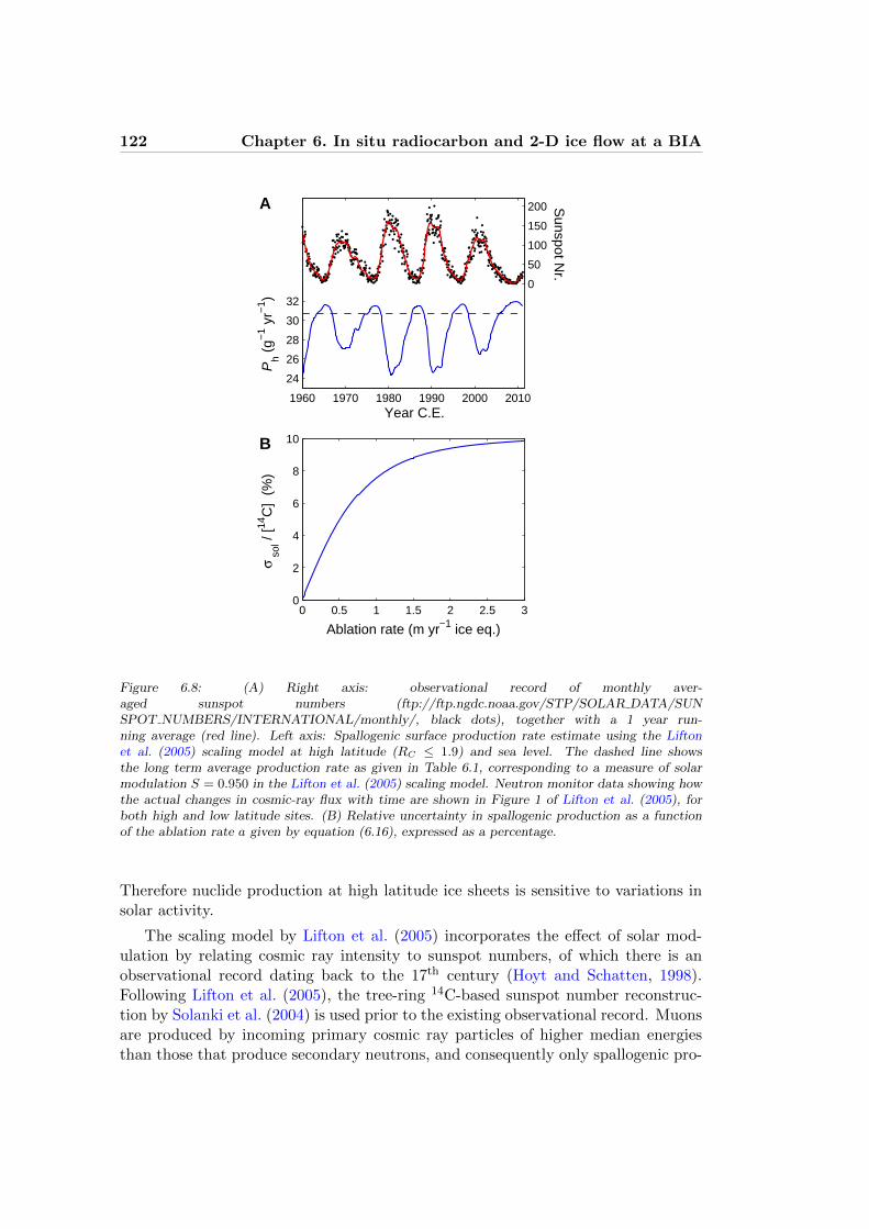
122 Chapter 6. In situ radiocarbon and 2-D ice flow at a BIA

0

50

100

150

200

1960 1970 1980 1990 2000 2010

24

26

28

30

32

Ph (

g−1 y

r−1 )

Year C.E.

0 0.5 1 1.5 2 2.5 30

2

4

6

8

10

Ablation rate (m yr−1 ice eq.)

σ sol

/ [14

C]

(%)

A

B

Sunspot N

r.

Figure 6.8: (A) Right axis: observational record of monthly aver-aged sunspot numbers (ftp://ftp.ngdc.noaa.gov/STP/SOLAR DATA/SUNSPOT NUMBERS/INTERNATIONAL/monthly/, black dots), together with a 1 year run-ning average (red line). Left axis: Spallogenic surface production rate estimate using the Liftonet al. (2005) scaling model at high latitude (RC ≤ 1.9) and sea level. The dashed line showsthe long term average production rate as given in Table 6.1, corresponding to a measure of solarmodulation S = 0.950 in the Lifton et al. (2005) scaling model. Neutron monitor data showing howthe actual changes in cosmic-ray flux with time are shown in Figure 1 of Lifton et al. (2005), forboth high and low latitude sites. (B) Relative uncertainty in spallogenic production as a functionof the ablation rate a given by equation (6.16), expressed as a percentage.

Therefore nuclide production at high latitude ice sheets is sensitive to variations insolar activity.

The scaling model by Lifton et al. (2005) incorporates the effect of solar mod-ulation by relating cosmic ray intensity to sunspot numbers, of which there is anobservational record dating back to the 17th century (Hoyt and Schatten, 1998).Following Lifton et al. (2005), the tree-ring 14C-based sunspot number reconstruc-tion by Solanki et al. (2004) is used prior to the existing observational record. Muonsare produced by incoming primary cosmic ray particles of higher median energiesthan those that produce secondary neutrons, and consequently only spallogenic pro-

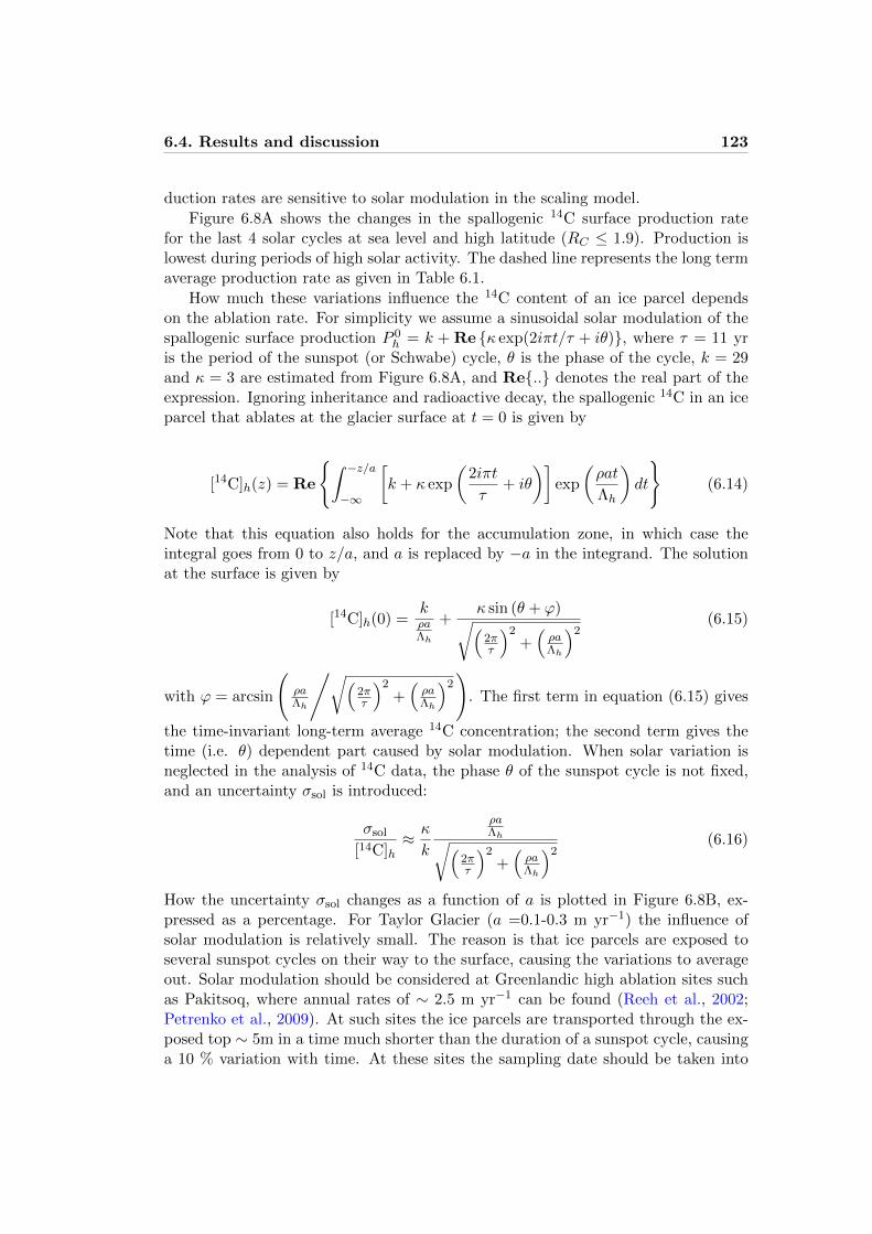
6.4. Results and discussion 123

duction rates are sensitive to solar modulation in the scaling model.

Figure 6.8A shows the changes in the spallogenic 14C surface production ratefor the last 4 solar cycles at sea level and high latitude (RC ≤ 1.9). Production islowest during periods of high solar activity. The dashed line represents the long termaverage production rate as given in Table 6.1.

How much these variations influence the 14C content of an ice parcel dependson the ablation rate. For simplicity we assume a sinusoidal solar modulation of thespallogenic surface production P 0

h = k + Re {κ exp(2iπt/τ + iθ)}, where τ = 11 yris the period of the sunspot (or Schwabe) cycle, θ is the phase of the cycle, k = 29and κ = 3 are estimated from Figure 6.8A, and Re{..} denotes the real part of theexpression. Ignoring inheritance and radioactive decay, the spallogenic 14C in an iceparcel that ablates at the glacier surface at t = 0 is given by

[14C]h(z) = Re

{∫ −z/a−∞

[k + κ exp

(2iπt

τ+ iθ

)]exp

(ρat

Λh

)dt

}(6.14)

Note that this equation also holds for the accumulation zone, in which case theintegral goes from 0 to z/a, and a is replaced by −a in the integrand. The solutionat the surface is given by

[14C]h(0) =kρaΛh

+κ sin (θ + ϕ)√(

2πτ

)2+(ρaΛh

)2(6.15)

with ϕ = arcsin

(ρaΛh

/√(2πτ

)2+(ρaΛh

)2)

. The first term in equation (6.15) gives

the time-invariant long-term average 14C concentration; the second term gives thetime (i.e. θ) dependent part caused by solar modulation. When solar variation isneglected in the analysis of 14C data, the phase θ of the sunspot cycle is not fixed,and an uncertainty σsol is introduced:

σsol

[14C]h≈ κ

k

ρaΛh√(

2πτ

)2+(ρaΛh

)2(6.16)

How the uncertainty σsol changes as a function of a is plotted in Figure 6.8B, ex-pressed as a percentage. For Taylor Glacier (a =0.1-0.3 m yr−1) the influence ofsolar modulation is relatively small. The reason is that ice parcels are exposed toseveral sunspot cycles on their way to the surface, causing the variations to averageout. Solar modulation should be considered at Greenlandic high ablation sites suchas Pakitsoq, where annual rates of ∼ 2.5 m yr−1 can be found (Reeh et al., 2002;Petrenko et al., 2009). At such sites the ice parcels are transported through the ex-posed top ∼ 5m in a time much shorter than the duration of a sunspot cycle, causinga 10 % variation with time. At these sites the sampling date should be taken into

124 Chapter 6. In situ radiocarbon and 2-D ice flow at a BIA

account when analyzing measued radiocarbon activities.

Solar modulation mostly influences the spallogenic production. Cosmogenic 14Cproduction at depths z > 5 m is dominated by muogenic production, and thereforeless sensitive to solar activity (and thereby sampling date). Consequently, for ab-lation sites solar modulation can be neglected at z > 5 m. For accumulation sitesthe solar variations in nuclide production are transported into the ice, and shouldalways be considered when accumulation is high.

6.4.3 Sensitivity of results to the main sources of uncertainty

Although solar modulation does not play a major role at Taylor Glacier, the mod-eled 14C concentrations are subject to a number of other uncertainties. We presenta sensitivity study comparing the magnitude of potential errors, the results of whichare shown in Figure 6.9A-C. The colors in the figure correspond to different sam-pling depths in the ice. We look at both the surface concentrations, as well asconcentrations at depths which are more suited for gas measurements (i.e. ice notsubjected to gas exchange through near-surface cracks, commonly observed at BIAs).

We analyze the three main sources of uncertainty: (1) the choice of strain rate pa-rameterization, (2) the ablation rate estimate based on measurements from a limitednumber of years, and (3) uncertainty in the cosmogenic production rates as foundin literature. For each plot the darker central lines give our modeled best estimatetotal cosmogenic 14C concentrations, whereas the shaded areas gives the uncertaintyestimate. Details are given in the figure caption. In our discussion of the sensitivitystudy, we shall focus on the part of the glacier that exposes the oldest ice, and istherefore most interesting for paleo-climate reconstructions (i.e. x < 35 km (Aciegoet al., 2007)).

The uncertainty contribution of the strain rate parameterization (Figure 6.9A)shows little depth dependence between the surface and z = 20 m. This is becausethe strain rates mostly influence the flow at depth, whereas the near-surface trajec-tories are fixed by the ablation rate and are only minorly influenced by strain rateuncertainties. The fact that the best estimate solution does not lie in the middleof the uncertainty band, but rather at the lower end, results from the exponentialdepth dependence of the nuclide production.

As long as the ablation uncertainty σa is small relative to the ablation rate a,the resulting uncertainty in 14C production is expected to be proportional to theamount of production itself as per equation (6.13). This is what is indeed observedfor x < 35 km where a is large (Figure 6.9B). As σa approaches a (i.e. for x > 35km), the uncertainty in 14C increases rapidly with increasing x.

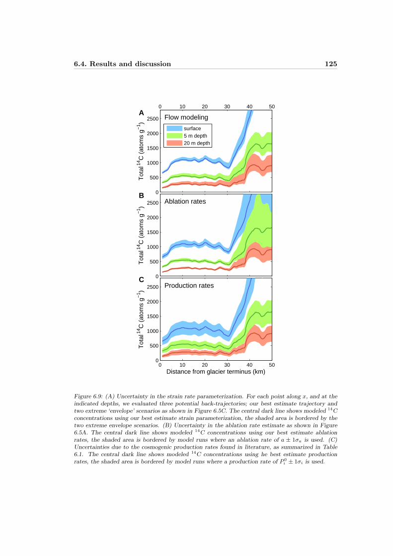
6.4. Results and discussion 125

0 10 20 30 40 50

0

500

1000

1500

2000

2500

Tot

al 14

C (

atom

s g−

1 )

Flow modeling

surface5 m depth20 m depth

0

500

1000

1500

2000

2500

Tot

al 14

C (

atom

s g−

1 )

Ablation rates

0 10 20 30 40 500

500

1000

1500

2000

2500

Distance from glacier terminus (km)

Tot

al 14

C (

atom

s g−

1 )

Production rates

A

B

C

Figure 6.9: (A) Uncertainty in the strain rate parameterization. For each point along x, and at theindicated depths, we evaluated three potential back-trajectories; our best estimate trajectory andtwo extreme ‘envelope’ scenarios as shown in Figure 6.5C. The central dark line shows modeled 14Cconcentrations using our best estimate strain parameterization, the shaded area is bordered by thetwo extreme envelope scenarios. (B) Uncertainty in the ablation rate estimate as shown in Figure6.5A. The central dark line shows modeled 14C concentrations using our best estimate ablationrates, the shaded area is bordered by model runs where an ablation rate of a ± 1σa is used. (C)Uncertainties due to the cosmogenic production rates found in literature, as summarized in Table6.1. The central dark line shows modeled 14C concentrations using he best estimate productionrates, the shaded area is bordered by model runs where a production rate of P 0

i ± 1σi is used.

126 Chapter 6. In situ radiocarbon and 2-D ice flow at a BIA

For all depths considered, the surface production rates as found in literature arethe largest source of uncertainty. In particular, the fast muon production rate has alarge uncertainty of about 60 % (Table 6.1). As shown in Fig 6.7C, the spallationcomponent is insignificant below 5 m depth. This implies that the deeper samples(5-20 m) collected at Taylor Glacier for 14C analyses during the 2010/2011 seasonwould allow us to improve substantially on the current estimates for muogenic 14Cproduction from 16O. Such improved production estimates would be important fornot just studies of 14C in ice, but would also be transferable to other materials, suchas e.g. quartz and carbonate rock used in exposure dating (Gosse and Phillips, 2001).

6.5 Summary and Conclusions

In this work we investigated in situ cosmogenic 14C production at ablation sites.First, we implemented a thermal neutron flux model for the air-ice interface, andfound that thermal neutron capture by nitrogen in air bubbles produces only negli-gible amounts of 14C.

Second, by modeling the trajectories of ice parcels at the center line of TaylorGlacier we calculated a best-estimate 14C concentration of ablating ice. We foundthat the commonly used ablation-only approximation by Lal et al. (1990) tends tounderestimate production as the ice flows down from parts of the glacier that havehigher production rates. For sections of the glacier where the basal topography isrugged, the ablation-only approximation deviates from the full model solution by upto 25%. This has important consequences when 14C activity measurements are usedto estimate ablation rates.

Third, we demonstrated that the influence of solar modulation is strongly de-pendent on ablation rate. At low ablation sites, such as Taylor Glacier, the effect issmall due to temporal averaging over several sunspot cycles. At high ablation sites,such as Pakitsoq, Greenland, solar modulation introduces an uncertainty of 10 % inthe spallogenic component. In these cases the sampling date needs to be consideredwhen interpreting data.

We introduced two methods to parameterize vertical strain rates with depth. Thefirst method is based on conservation of mass in the ice column; the second method isbased on measured surface strain rates. The second method proved to be less reliable,because (1) estimated surface strain rates from InSAR and GPS measurements showa poor correlation, (2) flow lines do not follow bedrock, and (3) mass is not conserved.

We presented a sensitivity study where we compare potential errors introducedby uncertainties in the strain rate parameterization, the ablation rates, and thepublished cosmogenic production rates. We found that the cosmogenic productionrates are the largest source of uncertainty. In the 2010/2011 Austral summer, Taylor

6.6. Acknowledgments 127

Glacier ice was sampled with the aim of constraining the cosmogenic productionrates more strongly, as well as determining the ratio of 14CH4 to 14CO producedin situ in the ice. By sampling at depths > 5 m the muogenic components can beisolated, which have the largest uncertainty in their production rates. The modelingresults presented here will aid us with the interpretation of 14C measurements onthese samples. Most importantly, this study will serve as a framework for correctingfuture 14CH4 measurements for the effect of in situ production with the purposeof reconstructing the true atmospheric signal. This would allow to answer pressingquestions about past changes in the global methane budget, such as whether marineclathrates can release large amounts of methane to the atmosphere.

6.6 Acknowledgments

We would like to thank Andy Bliss for his help on calculating ablation rates, Daniel Baggenstos for

measuring ablation stakes in the field and providing locations of the 2009-2010 sampling transect, and

Brent Goehring for fruitful discussions. C. Buizert would like to thank Thomas Blunier (Center for

Ice and Climate, University of Copenhagen), Bruce Vaughn and Jim White (INSTAAR, University

of Colorado) for their support and hospitality; V. V. Petrenko has been supported by the NOAA

Postdoctoral Fellowship in Climate and Global Change, NSF grants 0632222 and 0806387 (White)

and NSF grant 0839031 (Severinghaus); this work was partially supported by NSF grant OPP-

0125579 to K. M. Cuffey and NSF grant 0838936 to E. J. Brook; N. A. Lifton is grateful for support

by the CRONUS-Earth project (NSF EAR0345150) and the University of Arizona Accelerator Mass

Spectrometry Laboratory.

6.7 References

Aciego, S. M., Cuffey, K. M., Kavanaugh, J. L., Morse, D. L., and Severinghaus, J. P. (2007).Pleistocene ice and paleo-strain rates at taylor glacier, antarctica. Quaternary Res., 68:303–313.

Andree, M., Moor, E., Beer, J., Oeschger, H., Stauffer, B., Bonani, G., Hofmann, H., Morenzoni,E., Nessi, M., Suter, M., and Wolfli, W. (1984). C-14 dating of polar ice. Nucl. Instrum. Meth.B , 5(2):385–388.

Azuma, N., Nakawo, M., Higashi, A., and Nishio, F. (1985). Flow pattern near massif a in theyamato bare ice field estimated from the structures and the mechanical properties of a shallowice core. Memoirs of National Institute of Polar Research. Special issue, 39:173–183.

Bintanja, R. (1999). On the glaciological, meteorological, and climatological significance of Antarcticblue ice areas. Rev. Geophys., 37(3):337–359.

Bliss, A., Cuffey, K., and Kavanaugh, J. (2011). Sublimation and surface energy budget of taylorglacier, antarctica. J. Glaciol., in press.

Cuffey, K. and Paterson, W. S. B. (2010). The Physics of Glaciers, Fourth edition. Elsevier.De Jong, A., Alderliesten, C., Van der Borg, K., Van der Veen, C., and Van De Wal, R. (2004).

Radiocarbon analysis of the EPICA Dome C ice core: no in situ C-14 from the firn observed.Nucl. Instrum. Meth. B, 223:516–520.

Desilets, D. and Zreda, M. (2003). Spatial and temporal distribution of secondary cosmic-ray nucleonintensities and applications to in situ cosmogenic dating. Earth Planet. Sc. Lett., 206(1-2):21–42.

Desilets, D., Zreda, M., and Prabu, T. (2006). Extended scaling factors for in situ cosmogenicnuclides: New measurements at low latitude. Earth Planet. Sc. Lett., 246(3-4):265–276.

Dunai, T. J. (2000). Scaling factors for production rates of in situ produced cosmogenic nuclides: acritical reevaluation. Earth Planet. Sc. Lett., 176:157–169.

128 Chapter 6. In situ radiocarbon and 2-D ice flow at a BIA

Dunbar, N. W., McIntosh, W. C., and Esser, R. P. (2008). Physical setting and tephrochronologyof the summit caldera ice record at Mount Moulton, West Antarctica. Geol. Soc. Am. Bull.,120(7-8):796–812.

Fireman, E. and Norris, T. (1982). Ages and composition of gas trapped in Allan-Hills and Byrdcore ice. Earth Planet. Sc. Lett., 60(3):339–350.

Gosse, J. C. and Phillips, F. M. (2001). Terrestrial in situ cosmogenic nuclides: theory and appli-cation. Quaternary Sci. Rev., 20:1475–1560.

Grinsted, A., Moore, J., Spikes, V. B., and Sinisalo, A. (2003). Dating antarctic blue ice areas usinga novel ice flow model. Geophys. Res. Lett., 30(19):5.

Heisinger, B., Lal, D., Jull, A. J. T., Kubik, P., Ivy-Ochs, S., Knie, K., and Nolte, E. (2002a).Production of selected cosmogenic radionuclides by muons: 2. capture of negative muons. EarthPlanet. Sc. Lett., 200(3-4):357–369.

Heisinger, B., Lal, D., Jull, A. J. T., Kubik, P., Ivy-Ochs, S., Neumaier, S., Knie, K., Lazarev, V.,and Nolte, E. (2002b). Production of selected cosmogenic radionuclides by muons 1. fast muons.Earth Planet. Sc. Lett., 200(3-4):345–355.

Hoyt, D. V. and Schatten, K. H. (1998). Group sunspot numbers: A new solar activity reconstruc-tion. Sol. Phys., 181:491–491.

Jenk, T. M., Szidat, S., Schwikowski, M., Gaeggeler, H. W., Wacker, L., Synal, H.-A., and Saurer,M. (2007). Microgram level radiocarbon (C-14) determination on carbonaceous particles in ice.Nucl. Instrum. Meth. B, 259(1):518–525.

Jull, T. A. J., Lal, D., Donahue, D. J., Mayewski, P., Lorius, C., Raynaud, D., and Petit, J. R.(1994). Measurements of cosmic-ray-produced 14c in firn and ice from antarctica. Nucl. Instrum.Meth. B, 92:326–330.

Kavanaugh, J. L. and Cuffey, K. M. (2009). Dynamics and mass balance of taylor glacier, antarctica:2. force balance and longitudinal coupling. J. Geophys. Res.-Earth, 114:11.

Kavanaugh, J. L., Cuffey, K. M., Morse, D. L., Bliss, A. K., and Aciego, S. M. (2009a). Dynamicsand mass balance of taylor glacier, antarctica: 3. state of mass balance. J. Geophys. Res.-Earth,114:7.

Kavanaugh, J. L., Cuffey, K. M., Morse, D. L., Conway, H., and Rignot, E. (2009b). Dynamicsand mass balance of taylor glacier, antarctica: 1. geometry and surface velocities. J. Geophys.Res.-Earth, 114:15.

Lal, D. (1991). Cosmic-ray labeling of erosion surfaces - in situ nuclide production-rates and erosionmodels. Earth Planet. Sc. Lett., 104(2-4):424–439.

Lal, D., Jull, A., Donahue, D., Burr, G., Deck, B., Jouzel, J., and Steig, E. (2001). Record ofcosmogenic in situ produced C-14 in Vostok and Taylor Dome ice samples: Implications forstrong role of wind ventilation processes. J. Geophys. Res.-Atm., 106(D23):31933–31941.

Lal, D., Jull, A. J. T., Burr, G. S., and Donahue, D. J. (2000). On the characteristics of cosmogenicin situ c-14 in some gisp2 holocene and late glacial ice samples. Nucl. Instrum. Meth. B, 172:623–631.

Lal, D., Jull, A. J. T., Donahue, D. J., Burtner, D., and Nishiizumi, K. (1990). Polar ice ablationrates measured using in situ cosmogenic c-14. Nature, 346(6282):350–352.

Lal, D., Nishiizumi, K., and Arnold, J. R. (1987). In situ cosmogenic h-3, c-14 and be-10 for deter-mining the net accumulation and ablation rates of ice sheets. J. Geophys. Res.-Solid, 92(B6):4947–4952.

Lifton, N. A., Bieber, J. W., Clem, J. M., Duldig, M. L., Evenson, P., Humble, J. E., and Pyle,R. (2005). Addressing solar modulation and long-term uncertainties in scaling secondary cosmicrays for in situ cosmogenic nuclide applications. Earth Planet. Sc. Lett., 239:140–161.

Liu, B., Phillips, F. M., Fabryka-Martin, J. T., Fowler, M. M., and Stone, W. D. (1994). Cosmogeniccl-36 accumulation in unstable landforms 1. effects of the thermal neutron distribution. WaterResources Res., 30(11):3115–3125.

Moore, J. C., Nishio, F., Fujita, S., Narita, H., Pasteur, E., Grinsted, A., Sinisalo, A., and Maeno, N.(2006). Interpreting ancient ice in a shallow ice core from the south yamato (antarctica) blue icearea using flow modeling and compositional matching to deep ice cores. J. Geophys. Res.-Atm.,111:17.

6.7. References 129

Mughabghab, S., Divadeenam, M., and Holden, N. E. (1992). Neutron Resonance Parameters andThermal Cross Sections. Academic Press, New York.

Nesterenok, A. V. and Naidenov, V. O. (2009). Radiocarbon in the antarctic ice: The formation ofthe cosmic ray muon component at large depths. Geomagn. Aeronomy, 50:134–140.

Petrenko, V., Severinghaus, J., Brook, E., Reeh, N., and Schaefer, H. (2006). Gas records fromthe West Greenland ice margin covering the Last Glacial Termination: a horizontal ice core.Quaternary Sci. Rev., 25(9-10):865–875.

Petrenko, V. V., Severinghaus, J. P., Brook, E. J., Muhle, J., Headly, M., Harth, C. M., Schaefer,H., Reeh, N., Weiss, R. F., Lowe, D., and Smith, A. M. (2008). A novel method for obtainingvery large ancient air samples from ablating glacial ice for analyses of methane radiocarbon. J.Glaciol., 54(185):233–244.

Petrenko, V. V., Smith, A. M., Brook, E. J., Lowe, D., Riedel, K., Brailsford, G., Hua, Q., Schaefer,H., Reeh, N., Weiss, R. F., Etheridge, D., and Severinghaus, J. P. (2009). (ch4)-c-14 measurementsin greenland ice: Investigating last glacial termination ch4 sources. Science, 324:506–508.

Phillips, F. M., Stone, W. D., and Fabryka-Martin, J. T. (2001). An improved approach to calcu-lating low-energy cosmic-ray neutron fluxes near the land/atmosphere interface. Chem. Geol.,175(3-4):689–701.

Reeh, N., Oerter, H., and Thomsen, H. (2002). Comparison between Greenland ice-margin andice-core oxygen-18 records. Ann. Glaciol., 35:136–144.

Schaefer, H., Petrenko, V. V., Brook, E. J., Severinghaus, J. P., Reeh, N., Melton, J. R., andMitchell, L. (2009). Ice stratigraphy at the Pakitsoq ice margin, West Greenland, derived fromgas records. J. Glaciol., 55(191):411–421.

Sears, V. F. (1992). Neutron scattering lengths and cross sections. Neutron news, 3(3):26–37.Sinisalo, A. and Moore, J. C. (2010). Antarctic blue ice areas - towards extracting palaeoclimate

information. Antarct. Sci., 22(2):99–115.Smith, A. M., Levchenko, V. A., Etheridge, D. M., Lowe, D. C., Hua, Q., Trudinger, C. M., Zoppi,

U., and Elcheikh, A. (2000). In search of in-situ radiocarbon in law dome ice and firn. Nucl.Instrum. Meth. B, 172:610–622.

Solanki, S., Usoskin, I., Kromer, B., Schussler, M., and Beer, J. (2004). Unusual activity of the Sunduring recent decades compared to the previous 11,000 years. Nature, 431(7012):1084–1087.

Steig, E. J., Morse, D. L., Waddington, E. D., Stuiver, M., Grootes, P. M., Mayewski, P. A.,Twickler, M. S., and Whitlow, S. I. (2000). Wisconsinan and holocene climate history from anice core at taylor dome, western ross embayment, antarctica. Geogr. Ann. A, 82A:213–235.

Stone, J. O. (2000). Air pressure and cosmogenic isotope production. Journal of GeophysicalResearch-Solid Earth, 105(B10):23753–23759.

Van de Wal, R., Van Roijen, J., Raynaud, D., Van der Borg, K., De Jong, A., Oerlemans, J.,Lipenkov, V., and Huybrechts, P. (1994). From C-14/C-12 measurements towards radiocarbondating of ice. Tellus B, 46(2):94–102.

Van de Wal, R. S. W., Meijer, H. A. J., De Rooij, M., and Van der Veen, C. (2007). Radiocarbonanalyses along the EDML ice core in Antarctica. Tellus B, 59(1):157–165.

Van der Borg, K., Van der Kemp, W., Alderliesten, C., De Jong, A., and Lamers, R. (2001). In-situradiocarbon production by neutrons and muons in an antarctic blue ice field at Scharffenberg-botnen: A status report. Radiocarbon, 43(2B, Part 2):751–757.

Van Der Kemp, W., Alderliesten, C., Van Der Borg, K., De Jong, A., Lamers, R., Oerlemans, J.,Thomassen, M., and Van De Wal, R. (2002). In situ produced C-14 by cosmic ray muons inablating Antarctic ice. Tellus B, 54(2):186–192.

Van Roijen, J., Van der Borg, K., De Jong, A., and Oerlemans, J. (1995). A correction for in-situC-14 in Antarctic ice with (CO)-C-14. Radiocarbon, 37(2):165–169.

Wagemans, J., Wagemans, C., Goeminne, G., and Geltenbort, P. (2000). Experimental determina-tion of the 14n(n, p)14c reaction cross section for thermal neutrons. Phys. Rev. C, 61(6):064601.

130 Chapter 6. In situ radiocarbon and 2-D ice flow at a BIA

List of publications

Koppens, F. H. L., Buizert, C., Tielrooij, K. J., Vink, I. T., Nowack, K. C., Meunier,T., Kouwenhoven, L. P., and Vandersypen, L. M. K. (2006). Driven coherentoscillations of a single electron spin in a quantum dot. Nature, 442(7104):766–771.

Koppens, F. H. L., Buizert, C., Vink, I. T., Nowack, K. C., Meunier, T., Kouwen-hoven, L. P., and Vandersypen, L. M. K. (2007). Detection of single electron spinresonance in a double quantum dot. J. Appl. Phys., 101(8).

Buizert, C., Oiwa, A., Shibata, K., Hirakawa, K., and Tarucha, S. (2007). Kondouniversal scaling for a quantum dot coupled to superconducting leads. Phys. Rev.Lett., 99(13).

Shibata, K., Buizert, C., Oiwa, A., Hirakawa, K., and Tarucha, S. (2007). Lateralelectron tunneling through single self-assembled InAs quantum dots coupled tosuperconducting nanogap electrodes. Appl. Phys. Lett., 91(11).

Buizert, C., Koppens, F. H. L., Pioro-Ladriere, M., Tranitz, H.-P., Vink, I. T.,Tarucha, S., Wegscheider, W., and Vandersypen, L. M. K. (2008). In Situ Reduc-tion of Charge Noise in GaAs/AlxGa1−xAs Schottky-Gated Devices. Phys. Rev.Lett., 101(22).

Buizert, C., Martinerie, P., Petrenko, V. V., Severinghaus, J. P., Trudinger, C. M.,Witrant, E., Rosen, J. L., Orsi, A. J., Rubino, M., Etheridge, D. M., Steele,L. P., Hogan, C., Laube, J. C., Sturges, W. T., Levchenko, V. A., Smith, A. M.,Levin, I., Conway, T. J., Dlugokencky, E. J., Lang, P. M., Kawamura, K., Jenk,T. M., White, J. W. C., Sowers, T., Schwander, J., and Blunier, T. (2011). Gastransport in firn: multiple-tracer characterisation and model intercomparison forneem, northern greenland. Atmos. Chem. Phys. Discuss., 11:15975–16021.

Sapart, C. J., van der Veen, C., Vigano, I., Brass, M., van de Wal, R. S. W., Bock,M., Fischer, H., Sowers, T., Buizert, C., Sperlich, P., Blunier, T., Behrens, M.,Schmitt, J., Seth, B., and Rockmann, T. (2011). Simultaneous stable isotopeanalysis of methane and nitrous oxide on ice core samples. Atmos. Meas. Tech.Discuss., 4(4):4473–4503.

Buizert, C. Studies of firn air. In Elias, S. A., editor, submitted as invited chapterfor: Encyclopedia of Quaternary Sciences, 2nd Edition. Elsevier.

Buizert, C., Petrenko, V. V., Kavanaugh, J. L., Cuffey, K. M., Lifton, N. A. Brook,

131

132 Chapter 6. In situ radiocarbon and 2-D ice flow at a BIA

E. J., and Severinghaus, J. P. In situ cosmogenic radiocarbon production and2-d ice flow line modeling for an antarctic blue ice area. submitted to J. Geophys.Res.-Earth.

Hietanen, S., Jantti, H., Buizert, C., Jurgens, K., Labrenz, M., Voss, M., , andKuparinena, J. Hypoxia and nitrogen processing in the baltic sea water column.submitted to Limnol. Oceanogr.

Special thanks

Although this thesis should reflect what I did during my PhD, it does not come closeto capturing the full experience of my time in Copenhagen. The thesis is arguably alittle dull and hard to get through; the last three years have been rather the opposite:great fun, and gone by way too fast. While I take full responsibility for the state ofthe thesis, I have to credit others for all the good times.

The CIC (Center for Ice and Climate / Cake, Ice and Coffee) has been a wonderfulcommunity to be a part of. It has not only given me many great colleagues, but alsogood friends. First of all I want to thank my advisor (doctorvater) Thomas for hishelp and support throughout these last three years; I knew you were always therefor me. Various gaslab members, myself included, failed to ever fully adapt to theSwiss time zone, though. Also thanks to Dorthe for having done so much to makethe CIC the wonderful place that it is.

There are many other people at the CIC who deserve a special word of thanks.In particular Peter, who I have known as a roommate, mass-spec mechanic, cheesefondue accomplice, family guy and friend (not necessarily in that order). Althoughlabwork was often frustrating, we mostly kept a good spirit and laughed a lot. Iam leaving exactly at the moment you got the setup running (knock on wood); youdeserve those data more than anyone else. I look forward to spending much moretime with you and Colleen in the future. If I ever find out you’ll have a secondwedding in New Zealand, I hereby invite myself. High up on any list should beSigfus and Palla, who have treated me like family during the last three years. Fiveminutes after meeting them for the very first time I was invited to their summerhouse, where the beers and grilled Icelandic lamb were as abundant as their hos-pitality. Or in the words of Sigfus: “You are so welcome, you cannot believe it”.Thank you so very much. Ivana, we all know that behind your lovely sarcasm hidesa very sweet person, and most probably you will be both grumpy and charmed whenreading this. Once you left to Berkeley I turned soft, like Paul McCartney withoutLennon. I hope to meet His Imperial Highness one day. Christopher, it was a ton offun hanging out with you in Greenland, Greece and of course Copenhagen. I hope

133

134 Chapter 6. In situ radiocarbon and 2-D ice flow at a BIA

you’ll get your Master’s degree soon (it would be about time). Myriam, ever since Iheard you playing the harp in Utrecht I knew you were a special person. I am surean angel like you can find it in her heart to forgive us our stupid jokes (I still thinkthe CPR/herring joke is hilarious). Theo, it’s been a pleasure getting to know you,Tanina and little Naja. She is a lucky girl with such awesome parents. Jesper, Ihave always loved your Nordic sense of humor. I should have been homeless muchearlier on in my PhD; I got to know you (and Amager) much better in this lastweek sleeping on your couch. Thanks for offering your place to crash. Please tellDarling that I will miss him. Trev, I would listen to 70’s rock LPs, ride the metrofor hours, and ruin Mauro’s dinner parties with you any day of the week. Come tothink of it, for a few months that’s pretty much what we did any day of the week.Mads, I know she already said this, but you were often the most hilarious person inthe building. I still haven’t found the secret bacon message in your paper. Anne,thanks for all the good times on the ice and in Boulder. All the best with Kasperand the baby. Steff, you are a bad ass. Ever since you spent one hour showingholiday pictures and explaining biker’s slang at an official CIC meeting you are myhero. You also impressed me in the field by filing less than 100 µm off a drillhead,after which we went from empty to full barrels. Thanks also to Vasileos, who isjust as stubborn as I am. I can’t remember what we were arguing about the otherday, but I was right! I loved our stay in Litohoro. I left you a graduation present;don’t open it until you have defended you thesis. BF Italian, I cannot believe youhave been crushing my balls for three years now. Before you showed me what RealCulture is like, I was a barbarian using garlic and onion in the same dish. Sorry formaking you sleep in the closet. Corentin: your Karthaus year was definitely the mostfun, and I blame you. The glass pyramid was not our brightest moment. Thanksfor making me look punctual, by arriving even later at GasLab meetings than Idid. I hope you find what you are looking for. Ernesto, wat heerlijk om toch nogmet iemand Nederlands te kunnen praten. Vooral iemand die zo veel van taal (enbackgammon!) houdt. Heel veel succes in Gent. Michelle, I don’t think you realizehow infinitely funny you can be. Hope to see you in the States next year. Thanks toLone for her happy smiles in the morning; to Sebastian, my awesome officemate andthe only other person in town who cares about firn; to Hans Christian for lookingso mantastic in every possible situation; to Mai, with whom I shared the stress ofthesis writing in the last weeks; to Paul for his Aussie slang lessons; David for ’avingthe same ridiculous accent and for letting me run naked through his yard; Sune forhis great jokes and skill in fighting the bureaucrats; and to all the other lovely peo-ple at the CIC that I did not mention here, even though they deserve it just as much.

During my stay in Copenhagen I have been blessed with the sweetest roommatesone can wish for. First there was Arantxa, who technically never lived with us butmade herself very much at home all the same. Then there were the many incarnationsof the Gypsy family; some of the best roommates in the history of house sharing.Even though our housing was never cheap, sound-proof or well furnished, I wouldn’twant to live anywhere else. The cast, in order of appearance: Jay D.B. Armas, the

6.7. References 135

only person I know who can run a bar, edit a magazine, organize a lecture series,do a PhD, have three (presumably open-minded) girlfriends, write a book and sailacross the Atlantic all at the same time. Never a dull moment. Lars, a mixologist,entrepreneur, and blissfully irresponsible spirit; always up for jiggery-pokery of anykind. You still owe me money! Christina, architect and furniture designer. You werealways such a pleasure to have around, we never really recovered after you left. Ihope you can get into the PhD. Lucas, musician by day, barman by night. It wasmy pleasure. All the best with your music, and I told you I wouldn’t crash yourmoped! Carmen, our pig-nose-bacteria veterinarian and illicit film distributor. I amyour biggest fan and enjoyed all the time we spent together (which was a lot towardsthe end!) Fillipe is the dumbest idiot in the world for letting you go. And last butnot least, My: Train driver by day and musician by night, sweet on the outside, butfond of arm wrestling on the inside. I will miss you all.

During my PhD I had the pleasure of spending 5 months in Boulder, Coloradoat the Institute of Arctic and Alpine Research. Thanks to Bruce and Jim for theirsupport and help. Gentlemen, I had a great time at your lab. Vas, thanks forthe cross-country skiing lessons, the many great parties you threw and of coursefor inviting me to join the fieldwork at Taylor Glacier. I am happy to know we’llhave many more opportunities to work together in the near future. All the bestin Rochester with Christie and the cats. Thanks also to Emily, the only person inBoulder who understands that bike rides are more fun without spandex and with anice cold beer in the middle. Tyler, thanks for all the good times and the campingtrip. Still the absolute highlight of my stay in Boulder is not scientific. Thank youErica, for walking into our kitchen and into my life that summer evening. It makesme very happy to know that next year the Atlantic will shrink, and I can be withyou every day.

The life of a scientist involves (too?) much travel, and it’s not always easy tolive far away from friends and family. I want to thank my parents and my threewonderful sisters, Dineke, Petra and Annemiek. Dineke, I am very excited to knowI will be an uncle soon, and I wish you much strength in the coming months. I willbe there in April to meet my little niece or nephew. I also want to thank all of mymany good friends back in Holland. For all of you back home: I have not seen youas much as I would have liked to, but I will keep trying!

This all goes to show that, in a figurative sense, no thesis is written on an island.In a very literal sense, much of this thesis was written on an actual island (noteto Danish readers: Sjælland is not really an island). I am very grateful to MariaMatos Nascimento for letting me stay for one month in her beautiful old house inHorta, Faial on the Azorean Archipelago. The Azorean abundance of isolation andinsolation kept me both focused and, more importantly, tanned.

136 Chapter 6. In situ radiocarbon and 2-D ice flow at a BIA

Appendices

137

AGas transport in firn – Supplement

C. Buizert, P. Martinerie, V. V. Petrenko, J. P. Severinghaus,C. M. Trudinger, E. Witrant, J. L. Rosen, A. J. Orsi, M. Rubino,

D. M. Etheridge, L. P. Steele, C. Hogan, J. C. Laube,W. T. Sturges, V. A. Levchenko, A. M. Smith, I. Levin,

T. J. Conway, E. J. Dlugokencky, P. M. Lang, K. Kawamura,T. M. Jenk, J. W. C. White, T. Sowers, J. Schwander and

T. Blunier1

A.1 Introduction

This appendix is the supplement to Buizert et al. (2011), which has been included as Chapter 3in this thesis. It aims to provide more background information on the methods, as well as presentadditional modeling results which were omitted in the main article to improve readability. Mostresults from the US borehole are presented here.

The structure of this document closely follows that of the main text. Sections marked with anasterisk (∗) in the main article have a corresponding section here, where additional information canbe found.

A.2 Methods

A.2.1 NEEM 2008 firn air campaign

The location of the North Greenland Eemian ice drilling project (NEEM) camp and the site of the2008 firn air campaign are shown in Fig. A.1. For the sampling a 16 kW generator was placed at80 m distance downwind. In order to minimise air contamination, vehicles were parked near thegenerator and within the last 80 m all equipment was transported by manhauling. Drilling wasperformed alternatively in both holes with the Danish electromechanical shallow drill. The hole

1This appendix has been published as the supplement to C.Buizert et al.: Gas transport infirn: multiple-tracer characterisation and model intercomparison for NEEM, Northern Greenland.,Atmos. Chem. Phys. Discuss. 11:15975-6021 (2011).

139

140 Chapter A. Gas transport in firn – Supplement

Longitude (oW)

Latitud

e (o N

)

Prevailing

Wind

Figure A.1: Location of NEEM main structures and the site of the 2008 firn air campaign. Theinset shows the position of the NEEM camp in Northern Greenland.

diameter is 103.6 mm. In order to have an undisturbed surface for the first sampling levels, the first10 m were drilled with a hand auger producing the same diameter core and hole.

Table A.1 lists the sampling depths on both boreholes.

A.2.2 Physical characterisation of NEEM firn air site

For the density profile we use a fit to the NEEM main core density data averaged over 0.55msegments (Johnsen, personal communication, 2009). For the three stages of densification (Arnaudet al., 2000) we use a separate fit. Data fitting was done by eye, and care was taken that thesecond derivative is continuous over the transitions between the stages. Surface density was chosenas ρ = 0.35 g cm−3. The density fit is given by

ρ = a1 + a2z + a3ea4(16−z) for z < 16m

ρ = a5 + a6z + a7z2 for 16 ≤ z < 110m (A.1)

ρ = a8 + a9

(1 − ea10(z−110)

)for z ≥ 110m

The constants in Eq. (A.1) obtained in the fitting procedure can be found in Table A.2. Thedensity data together with the fit are shown in Fig. 1 of the main document.

We use the closed porosity parameterisation of Goujon et al. (2003):

scl = 0.37s

(s

sco

)−7.6

(A.2)

with sco the close-off porosity consistent with the mean close-off density relation by Martinerieet al. (1994). Changing sco results in changing the complete close-off depth (sop = 0). Field dataindicate the last successful air pumping depth in firn and a depth at which no air could be extracted.The depth at which open firn porosity becomes zero should be located in this interval. Using themean close-off density of Martinerie et al. (1994) in Eq. (A.2) generally gives a complete close-off

A.2. Methods 141

Table A.1: Firn air sampling depths in meters for the EU (S2) and US (S3) boreholes.

Level EU depth (m) US depth (m)

0 0.00 0.001 2.50 2.852 4.90 5.233 7.55 9.834 10.10 19.305 14.80 34.706 19.75 49.707 27.54 57.478 34.72 59.909 42.42 62.0010 50.00 64.0311 54.90 65.5012 57.40 66.9013 59.90 68.3014 61.95 69.8015 63.85 71.4016 65.75 72.8517 68.05 73.8018 70.05 75.6019 72.00 -20 74.08 -21 75.90 -22 77.75 -

depth (sop = 0) inconsistent with field data. The cause of this discrepancy is not clear; it couldbe due to e.g. firn heterogeneity, or biases and uncertainties in firn density measurements. In thecase of NEEM, it leads to a complete close-off depth higher than the last measurement depth. Adifferent mean close-off density value is used in order to obtain a complete close-off depth consistentwith field data. At NEEM the last successful air pumping depth was z = 77.75 m; a decreased airflow (insufficient for sampling) was observed at z = 79 m depth. It was thus considered that airwas isolated from the atmosphere at that depth, and used 78.8m as the zero open porosity level,equivalent to a mean close-off density ρco = 0.8312 g cm−3. Note that sop is not necessarily zerobelow the deepest sampling depth (Aydin et al., 2010).The accumulation rate estimate is based on the dated NEEM 2007 shallow S1 core (Dahl-Jensen,personal communication, 2010). The derived variations of the accumulation rate with time areshown in Fig. A.2. For all the tracers we run the models from 1800 to the sampling date 2008.54.As a best estimate of the accumulation rate we use the mean value over this period of A = 0.216m yr−1 ice equivalent. The best estimate for the current day value is A = 0.227 m yr−1, which iswithin the range of variability observed in the past.

A.2.3 Gas measurements

For SF6, the IUP data (EU and US holes) have been rescaled by 0.9912 to place the data on theNOAA scale that we use in our atmospheric reconstructions (rescaling corresponds to a modernday offset of 0.06 ppt). The NOAA and UEA SF6 data were provided on the NOAA scale. Aftercorrecting the IUP data no inter-laboratory offsets were observed on either borehole.

For the US hole NOAA CH4 data have been used exclusively where available (13 depth levels).For a remaining 5 depths we have no NOAA measurements, and for these depths we have used IUPdata after scaling them in the following way to place them on the NOAA scale:

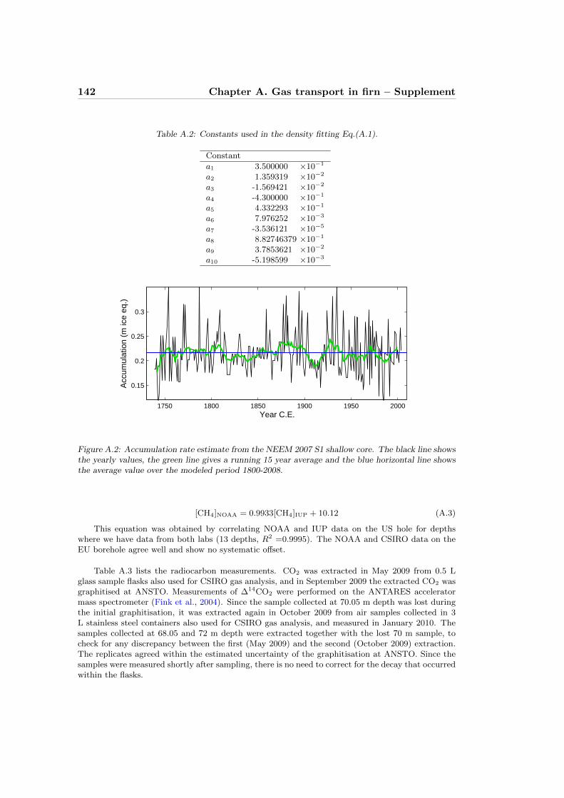
142 Chapter A. Gas transport in firn – Supplement

Table A.2: Constants used in the density fitting Eq.(A.1).

Constant

a1 3.500000 ×10−1

a2 1.359319 ×10−2

a3 -1.569421 ×10−2

a4 -4.300000 ×10−1

a5 4.332293 ×10−1

a6 7.976252 ×10−3

a7 -3.536121 ×10−5

a8 8.82746379 ×10−1

a9 3.7853621 ×10−2

a10 -5.198599 ×10−3

1750 1800 1850 1900 1950 2000

0.15

0.2

0.25

0.3

Acc

umul

atio

n (m

ice

eq.)

Year C.E.

Figure A.2: Accumulation rate estimate from the NEEM 2007 S1 shallow core. The black line showsthe yearly values, the green line gives a running 15 year average and the blue horizontal line showsthe average value over the modeled period 1800-2008.

[CH4]NOAA = 0.9933[CH4]IUP + 10.12 (A.3)

This equation was obtained by correlating NOAA and IUP data on the US hole for depthswhere we have data from both labs (13 depths, R2 =0.9995). The NOAA and CSIRO data on theEU borehole agree well and show no systematic offset.

Table A.3 lists the radiocarbon measurements. CO2 was extracted in May 2009 from 0.5 Lglass sample flasks also used for CSIRO gas analysis, and in September 2009 the extracted CO2 wasgraphitised at ANSTO. Measurements of ∆14CO2 were performed on the ANTARES acceleratormass spectrometer (Fink et al., 2004). Since the sample collected at 70.05 m depth was lost duringthe initial graphitisation, it was extracted again in October 2009 from air samples collected in 3L stainless steel containers also used for CSIRO gas analysis, and measured in January 2010. Thesamples collected at 68.05 and 72 m depth were extracted together with the lost 70 m sample, tocheck for any discrepancy between the first (May 2009) and the second (October 2009) extraction.The replicates agreed within the estimated uncertainty of the graphitisation at ANSTO. Since thesamples were measured shortly after sampling, there is no need to correct for the decay that occurredwithin the flasks.

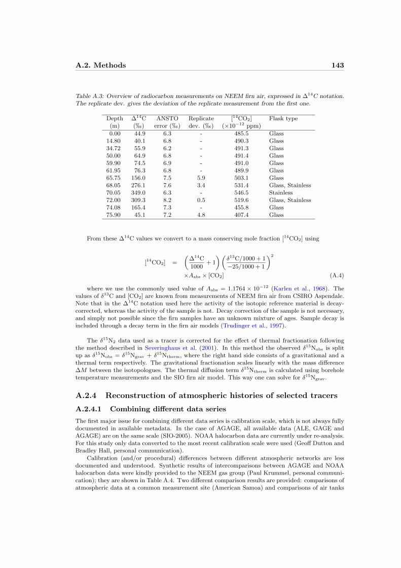
A.2. Methods 143

Table A.3: Overview of radiocarbon measurements on NEEM firn air, expressed in ∆14C notation.The replicate dev. gives the deviation of the replicate measurement from the first one.

Depth ∆14C ANSTO Replicate [14CO2] Flask type(m) (h) error (h) dev. (h) (×10−12 ppm)

0.00 44.9 6.3 - 485.5 Glass14.80 40.1 6.8 - 490.3 Glass34.72 55.9 6.2 - 491.3 Glass50.00 64.9 6.8 - 491.4 Glass59.90 74.5 6.9 - 491.0 Glass61.95 76.3 6.8 - 489.9 Glass65.75 156.0 7.5 5.9 503.1 Glass68.05 276.1 7.6 3.4 531.4 Glass, Stainless70.05 349.0 6.3 - 546.5 Stainless72.00 309.3 8.2 0.5 519.6 Glass, Stainless74.08 165.4 7.3 - 455.8 Glass75.90 45.1 7.2 4.8 407.4 Glass

From these ∆14C values we convert to a mass conserving mole fraction [14CO2] using

[14CO2] =

(∆14C

1000+ 1

)(δ13C/1000 + 1

−25/1000 + 1

)2

×Aabs × [CO2] (A.4)

where we use the commonly used value of Aabs = 1.1764 × 10−12 (Karlen et al., 1968). Thevalues of δ13C and [CO2] are known from measurements of NEEM firn air from CSIRO Aspendale.Note that in the ∆14C notation used here the activity of the isotopic reference material is decay-corrected, whereas the activity of the sample is not. Decay correction of the sample is not necessary,and simply not possible since the firn samples have an unknown mixture of ages. Sample decay isincluded through a decay term in the firn air models (Trudinger et al., 1997).

The δ15N2 data used as a tracer is corrected for the effect of thermal fractionation followingthe method described in Severinghaus et al. (2001). In this method the observed δ15Nobs is splitup as δ15Nobs = δ15Ngrav + δ15Ntherm, where the right hand side consists of a gravitational and athermal term respectively. The gravitational fractionation scales linearly with the mass difference∆M between the isotopologues. The thermal diffusion term δ15Ntherm is calculated using boreholetemperature measurements and the SIO firn air model. This way one can solve for δ15Ngrav.

A.2.4 Reconstruction of atmospheric histories of selected tracers

A.2.4.1 Combining different data series

The first major issue for combining different data series is calibration scale, which is not always fullydocumented in available metadata. In the case of AGAGE, all available data (ALE, GAGE andAGAGE) are on the same scale (SIO-2005). NOAA halocarbon data are currently under re-analysis.For this study only data converted to the most recent calibration scale were used (Geoff Dutton andBradley Hall, personal communication).

Calibration (and/or procedural) differences between different atmospheric networks are lessdocumented and understood. Synthetic results of intercomparisons between AGAGE and NOAAhalocarbon data were kindly provided to the NEEM gas group (Paul Krummel, personal communi-cation); they are shown in Table A.4. Two different comparison results are provided: comparisons ofatmospheric data at a common measurement site (American Samoa) and comparisons of air tanks

144 Chapter A. Gas transport in firn – Supplement

Table A.4: Concentration ratios (NOAA/AGAGE) for halocarbon species.Species Multiple sitesa,b Samoaa IHALACEc This study Scales Comment

flask/in-situ in-situ/in-situ (prelim.IHALACE)CFC-11 1.0100 1.0095 1.0058 1.0081 NOAA-1993/SIO-05 time dependentCFC-11 1.0057 1.0080 - 1.0081 NOAA-1993/SIO-05 2007-2009 onlyCFC-12 0.9973 0.9965 0.9978 0.9978 NOAA-2008/SIO-05CFC-113 1.0199 1.0251 1.0266 1.0215 NOAA-2003/SIO-05

CH3CCl3 1.0339 1.0379 1.0572 / - d 1.0627 / 1.0526d NOAA-2003/SIO-05 ECD detector

CH3CCl3 1.0158 - 1.0081 / - d 1.0081 / 1.0030d NOAA-2003/SIO-05 GCMS detectora Krummel, personal communicationb Based on Mace Head, Trinidad Head, Samoa and Cape Grimc Hall, B.D., Engle, A., Muhle, J., Elkins, J. et al., Results from the International Halocarbons in Air Comparison Experiment(IHALACE), in preparationd Ratios for tanks at 22 ppt and 18 ppt respectively

circulated around measurement labs (IHALACE: International HALocarbons in Air ComparisonExperiment; Bradley Hall, personal communication). The comparisons are consistent for CFC-12 and CFC-113. Concentration ratios at American Samoa are time-dependent for CFC-11. ForCH3CCl3 Samoa and IHALACE results are inconsistent (note that IHALACE tanks had low con-centration levels), and different results are obtained with Electron Capture Detector (ECD) and Gaschromatography–mass spectrometry (GCMS). As old trend data were obtained with ECD, GCMSmeasurements are not used for this species; a NOAA/AGAGE ratio of 1.035 is used.

A.2.4.2 Description of the reconstructions

CO2: Summit and Alert NOAA-ESRL monthly record from 6/1985 - 12/2008. For months whenboth Summit and Alert records are available we use the average of the two. For months when onlydata from either one of the stations is available that station is used, with a correction for the averageAlert-Summit offset for that given month. Mauna Loa (MLO) NOAA-ESRL (7/1976-5/1985) andSIO (3/1958-6/1976) records are used for indicated periods with a latitudinal correction appliedbased on the mean of the modern day MLO-Summit and MLO-Alert offset. Plots for offset vs. timerevealed no trend, so a constant correction is used. A months 2-4/1964 gap in the SIO MLO recordis filled by linear interpolation.

Prior to the MLO instrumental record, mean annual values are based on the the Law Domemean-annual 20-yr smoothed record (1832-1958) and the Law Dome 75-yr smoothed mean annualrecord (1800-1831) (Etheridge et al., 1996), corrected for the Law Dome-NEEM offset. For missingyears data points are interpolated linearly. Both the value and the trend of the Law Dome-NEEMoffset were determined for the period 1959-1978 where the records overlap. In 1931 this resultsin NEEM concentration equaling the Law Dome concentration, so the inter-polar gradient goes tozero. For simplicity, beyond this point we simply set NEEM equal to Law Dome. A seasonal CO2

cycle is added based on NEEM reconstructed monthly values for 1959-2008.

CH4: Summit and Alert NOAA-ESRL monthly record from 6/1985-12/2008. For months whenthe Summit record is available, NEEM is set equal to Summit. For months where Summit recordis unavailable, the NEEM reconstruction is based on Alert with a correction for the Summit-Alertoffset for that month applied. Alert-Summit offsets show no significant trends with time.

Prior to the Alert record mean annual values are based on the Law Dome firn record (1978-1985) and the Law Dome ice core record (1800-1978) (Etheridge et al., 1998), scaled by 1.0124to convert the data to the NOAA 2004 CH4 calibration scale, and with a correction applied forthe Law Dome-NEEM offset. The inter-polar gradient (IPG) is assumed to be constant at 45 ppbfrom 1800-1885 (Etheridge et al., 1998). For 1886-1985 it is assumed that the IPG is a function ofboth Law Dome [CH4] and d[CH4]/dt. The IPG correction is tuned to the period 1986-1998 wheredirect atmospheric measurements are available and there is an appreciable growth rate d[CH4]/dt.A seasonal CH4 cycle is added based on the reconstructed NEEM monthly values for 1986-2008.It is assumed that the amplitude of the seasonal cycle is directly proportional to the mean annualconcentration.

A.2. Methods 145

14CO2: The atmospheric 14CO2 record from Fruholmen, Norway, is used for its proximityto Greenland, from 1/1963-6/1993 (Nydal and Lovseth, 1996). Atmospheric measurements fromcentral Europe have been used from 6/1993-12/2008 (Vermunt and Jungfraujoch, Levin et al.,2008) and from 2/1959-12/1962 (Vermunt, Levin and Kromer, 2004). In the period 1990-2010the reconstruction agrees within a few per mil with a recent atmospheric record from Alert station(Levin et al., 2010b), which was not yet available at the time we finalised the reconstruction.

Southern hemisphere atmospheric 14CO2 measurements are used from 1954-1959 (Manning andMelhuish, 1994) with a correction of 30 h on average to account for the interhemispheric gradient.

Prior to 1955 no direct atmospheric records exist and the reconstruction is equal to ∆14CO2

reconstructed from dendrochronologically dated tree-ring samples (Reimer et al., 2004). The atmo-spheric ∆14CO2 has been converted to a ppm scale using Eq. (A.4).

It should be noted that, unlike the firn air 14C measurements, the atmospheric histories havebeen age-corrected for decay between the time that the sample was “collected” (in the case of trees,since the tree removed the CO2 from the air), and the time that the sample was measured.

δ13CO2: A δ13CO2 reconstruction is required to convert ∆14CO2 values from a permil scale toa mass-conserving ppm scale as described by Eq. (A.4). The Alert CSIRO monthly record from1/1990-6/2008 is used without correction.

Prior to the Alert record we use the Cape Grim air archive record (1978-1989) and the LawDome ice core record (1800-1978) (Francey et al., 1999), with a correction applied for the LawDome-NEEM offset. The correction is assumed to scale linearly with the atmospheric growth rateof CO2, and is calibrated to the period 1990-2008 where CSIRO Alert and Cape Grim monthlyrecords are available.

CFC-11: Emission-based model results from Martinerie et al. (2009) before 7/1978. MidNorthern latitudes combined AGAGE monthly record 7/1978-3/2009. Overall scenario convertedto NOAA scale with NOAA / AGAGE = 1.0081 (IHALACE).

CFC-12: Mid Northern latitudes combined AGAGE monthly record 1/1981- 3/2009 (earlyrecord ignored because of missing data and high inter-hemispheric gradient). 2D model results fromMartinerie et al. (2009) before. Overall scenario converted to NOAA scale with NOAA / AGAGE= 0.9978 (IHALACE).

CFC-113: Mid Northern latitudes combined AGAGE monthly record 6/1986- 3/2009 (earlyrecord ignored because of missing data and high inter-hemispheric gradient). Emission-based modelresults from Martinerie et al. (2009) before. Overall scenario converted to NOAA scale with NOAA/ AGAGE = 1.0215 (IHALACE).

SF6: Barrow NOAA-ESRL combined (Geoff Dutton) monthly record 1/1999- 7/2009 (Barrowdata for 1995-1998 ignored because of variable N/S gradient. Emission-based model results fromMartinerie et al. (2009) before.

CH3CCl3: Mid Northern latitudes combined AGAGE monthly record 7/1978- 3/2009. Emission-based model results before 7/1978 (visual rescaling by 1.05). Overall scenario converted to NOAAscale with a NOAA / AGAGE = 1.035 (Samoa data with ECD detection).

HFC-134a: Barrow NOAA monthly record 2/1995- 3/2009, Emission-based model results be-fore 02/1995 (visual rescaling by 1.10).

The mid-latitude AGAGE data could not be extrapolated to high latitudes for halocarbons.The first reason is the highly time dependent meridional concentration gradients; for species phasedout under the Montreal Protocol, due to strongly reduced emissions, even the inter-polar gradientis close to zero in recent years. Another difficulty arises from the fact that the NOAA-ESRL mid

146 Chapter A. Gas transport in firn – Supplement

Northern latitude site (Niwot Ridge) is a high altitude site, thus the effects of altitude and latitudeon concentrations cannot be separated.

δ15N-N2: There is no need for a δ15N-N2 reconstruction since the isotopic composition of Ni-trogen is constant in the atmosphere on the timescales considered here. Formally, calculating theisotopic ratio would require both 15N14N and 14N14N isotopologues to be modeled separately. How-ever, the 14N14N isotopologue constitutes nearly 80% of the air molecules, violating the assumptionused by the firn models of modeling diffusion of trace gases into air. We have instead chosen touse an atmospheric forcing [15N14N](t) = 1 for all t, and we assume that the 14N14N istopologuehas unity mixing ratio everywhere [14N14N](z) = 1. This is tantamount to assuming that 14N14N isthe only non-trace gas in air (molecular diffusivity of 15N14N into air is used, however, rather than15N14N into 14N14N). The δ15N-N2 signal is then given as δ15N-N2(z) = 103×([15N14N](z) − 1).

A.2.4.3 Uncertainty estimates on atmospheric reconstructions

Table A.5 summarises the elements used for the uncertainty estimates. The dates refer to the periodfor which the comparison was made (thus the uncertainty should be applied from the beginning ofthe earliest data series to the end date of the comparison). The biases between labs can be large andtime varying for halocarbons. To distinguish the mean bias from the variability of the differencesbetween data series, these variabilities are noted dev. instead of σ, because the distributions areobviously not Gaussian in many cases.

Uncertainties are overall much higher for halocarbons than for other gases. For halocarbons,uncertainties on emissions are likely more pessimistic than uncertainties on concentrations. As anillustration, Martinerie et al. (2009) rescaled halocarbon emissions so that modeled atmosphericconcentrations fit the early part of atmospheric datasets. Rescaling factors for CFC-11, CFC-12,CFC-113, CCl4 and SF6 range between 5 and 10% for the rising part of the trends.

Niwort Ridge halocarbon concentrations are mostly lower than Barrow concentrations, suggest-ing a dominant effect of altitude rather than latitude. Differences between Summit and Barrow aremuch lower. This suggests that the mid-latitude to Greenland concentration gradient is within thenoise on the data for halocarbons.

Using the values in Table A.5 uncertainties are constructed in the following way:

CO2 uncertainties: 1985-2008: half the ALT/SUM offset, 1976-1985: half the ALT/SUMoffset and the standard deviation of the ALT/MLO-NOAA offset, 1958-1976: half the ALT/SUMoffset and the standard deviation of the ALT/MLO-SIO offset, 1930-1958: twice the 1σ Law Domemeasurement uncertainty, the IPG uncertainty estimate, 1800-1930: three times the 1σ Law Domeuncertainty and the IPG uncertainty estimate. In each period the listed terms are added quadrati-cally to estimate the total uncertainty.

CH4 uncertainties: The CH4 uncertainty is dominated by the uncertainty in the IPG esti-mate, which is large for CH4. For this reason three independent reconstructions were made, and theuncertainty was taken as the maximum difference between the reconstructions. The first method isdescribed in Sect. A.2.4.2, a second method assumes the IPG is linearly related to the CH4 mixingratio, a third method uses the a linear regression analysis between atmospheric growth rate andIPG. The comparison leads to an uncertainty ranging from 5-42 ppb.

For halocarbons, expressing emission-related uncertainties in % results in an unrealistic zerouncertainty at the start date of emissions. Thus somewhat arbitrarily, a minimum absolute un-certainty (in ppt) was set to the present-day uncertainty. The large increase in uncertainty whenswitching from atmospheric records to emission based estimates is applied gradually (over about 2years) for all halocarbon species.

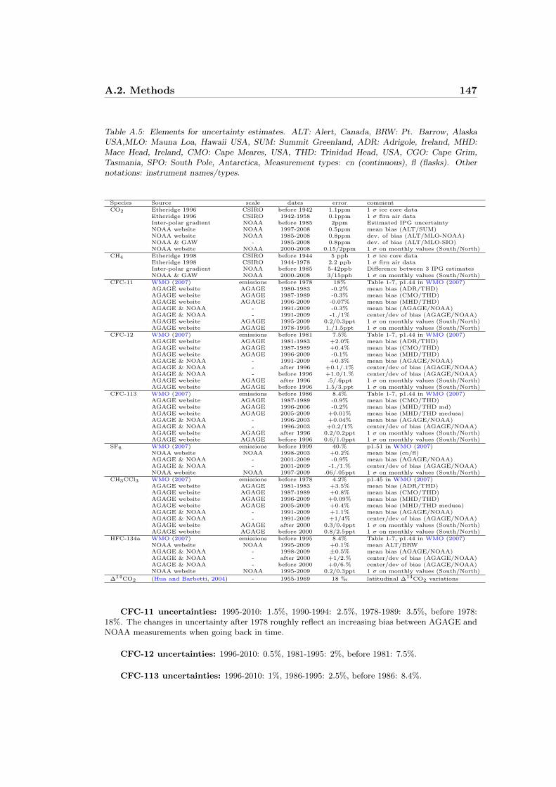
A.2. Methods 147

Table A.5: Elements for uncertainty estimates. ALT: Alert, Canada, BRW: Pt. Barrow, AlaskaUSA,MLO: Mauna Loa, Hawaii USA, SUM: Summit Greenland, ADR: Adrigole, Ireland, MHD:Mace Head, Ireland, CMO: Cape Meares, USA, THD: Trinidad Head, USA, CGO: Cape Grim,Tasmania, SPO: South Pole, Antarctica, Measurement types: cn (continuous), fl (flasks). Othernotations: instrument names/types.

Species Source scale dates error commentCO2 Etheridge 1996 CSIRO before 1942 1.1ppm 1 σ ice core data

Etheridge 1996 CSIRO 1942-1958 0.1ppm 1 σ firn air dataInter-polar gradient NOAA before 1985 2ppm Estimated IPG uncertaintyNOAA website NOAA 1997-2008 0.5ppm mean bias (ALT/SUM)NOAA website NOAA 1985-2008 0.8ppm dev. of bias (ALT/MLO-NOAA)NOAA & GAW - 1985-2008 0.8ppm dev. of bias (ALT/MLO-SIO)NOAA website NOAA 2000-2008 0.15/2ppm 1 σ on monthly values (South/North)

CH4 Etheridge 1998 CSIRO before 1944 5 ppb 1 σ ice core dataEtheridge 1998 CSIRO 1944-1978 2.2 ppb 1 σ firn air dataInter-polar gradient NOAA before 1985 5-42ppb Difference between 3 IPG estimatesNOAA & GAW NOAA 2000-2008 3/15ppb 1 σ on monthly values (South/North)

CFC-11 WMO (2007) emissions before 1978 18% Table 1-7, p1.44 in WMO (2007)AGAGE website AGAGE 1980-1983 -0.2% mean bias (ADR/THD)AGAGE website AGAGE 1987-1989 -0.3% mean bias (CMO/THD)AGAGE website AGAGE 1996-2009 -0.07% mean bias (MHD/THD)AGAGE & NOAA - 1991-2009 -0.3% mean bias (AGAGE/NOAA)AGAGE & NOAA - 1991-2009 -1./1% center/dev of bias (AGAGE/NOAA)AGAGE website AGAGE 1995-2009 0.2/0.3ppt 1 σ on monthly values (South/North)AGAGE website AGAGE 1978-1995 1./1.5ppt 1 σ on monthly values (South/North)

CFC-12 WMO (2007) emissions before 1981 7.5% Table 1-7, p1.44 in WMO (2007)AGAGE website AGAGE 1981-1983 +2.0% mean bias (ADR/THD)AGAGE website AGAGE 1987-1989 +0.4% mean bias (CMO/THD)AGAGE website AGAGE 1996-2009 -0.1% mean bias (MHD/THD)AGAGE & NOAA - 1991-2009 +0.3% mean bias (AGAGE/NOAA)AGAGE & NOAA - after 1996 +0.1/.1% center/dev of bias (AGAGE/NOAA)AGAGE & NOAA - before 1996 +1.0/1.% center/dev of bias (AGAGE/NOAA)AGAGE website AGAGE after 1996 .5/.6ppt 1 σ on monthly values (South/North)AGAGE website AGAGE before 1996 1.5/3.ppt 1 σ on monthly values (South/North)

CFC-113 WMO (2007) emissions before 1986 8.4% Table 1-7, p1.44 in WMO (2007)AGAGE website AGAGE 1987-1989 -0.9% mean bias (CMO/THD)AGAGE website AGAGE 1996-2006 -0.2% mean bias (MHD/THD md)AGAGE website AGAGE 2005-2009 +0.01% mean bias (MHD/THD medusa)AGAGE & NOAA - 1996-2003 +0.04% mean bias (AGAGE/NOAA)AGAGE & NOAA - 1996-2003 +0.2/1% center/dev of bias (AGAGE/NOAA)AGAGE website AGAGE after 1996 0.2/0.2ppt 1 σ on monthly values (South/North)AGAGE website AGAGE before 1996 0.6/1.0ppt 1 σ on monthly values (South/North)

SF6 WMO (2007) emissions before 1999 40.% p1.51 in WMO (2007)NOAA website NOAA 1998-2003 +0.2% mean bias (cn/fl)AGAGE & NOAA - 2001-2009 -0.9% mean bias (AGAGE/NOAA)AGAGE & NOAA - 2001-2009 -1./1.% center/dev of bias (AGAGE/NOAA)NOAA website NOAA 1997-2009 .06/.05ppt 1 σ on monthly values (South/North)

CH3CCl3 WMO (2007) emissions before 1978 4.2% p1.45 in WMO (2007)AGAGE website AGAGE 1981-1983 +3.5% mean bias (ADR/THD)AGAGE website AGAGE 1987-1989 +0.8% mean bias (CMO/THD)AGAGE website AGAGE 1996-2009 +0.09% mean bias (MHD/THD)AGAGE website AGAGE 2005-2009 +0.4% mean bias (MHD/THD medusa)AGAGE & NOAA - 1991-2009 +1.1% mean bias (AGAGE/NOAA)AGAGE & NOAA - 1991-2009 +1/4% center/dev of bias (AGAGE/NOAA)AGAGE website AGAGE after 2000 0.3/0.4ppt 1 σ on monthly values (South/North)AGAGE website AGAGE before 2000 0.8/2.5ppt 1 σ on monthly values (South/North)

HFC-134a WMO (2007) emissions before 1995 8.4% Table 1-7, p1.44 in WMO (2007)NOAA website NOAA 1995-2009 +0.1% mean ALT/BRWAGAGE & NOAA - 1998-2009 ±0.5% mean bias (AGAGE/NOAA)AGAGE & NOAA - after 2000 +1/2.% center/dev of bias (AGAGE/NOAA)AGAGE & NOAA - before 2000 +0/6.% center/dev of bias (AGAGE/NOAA)NOAA website NOAA 1995-2009 0.2/0.3ppt 1 σ on monthly values (South/North)

∆14CO2 (Hua and Barbetti, 2004) - 1955-1969 18 h latitudinal ∆14CO2 variations

CFC-11 uncertainties: 1995-2010: 1.5%, 1990-1994: 2.5%, 1978-1989: 3.5%, before 1978:18%. The changes in uncertainty after 1978 roughly reflect an increasing bias between AGAGE andNOAA measurements when going back in time.

CFC-12 uncertainties: 1996-2010: 0.5%, 1981-1995: 2%, before 1981: 7.5%.

CFC-113 uncertainties: 1996-2010: 1%, 1986-1995: 2.5%, before 1986: 8.4%.

148 Chapter A. Gas transport in firn – Supplement

SF6 uncertainties: 1999-2010: 1.5%, 1985-1998: 3.5% South. Hem. and 5% North. Hem.,1978-1984: 3.5% South. Hem. and 10% North. Hem., before 1978: 40%. The high uncertaintyon emissions reflects mismatches between bottom-up and top-down estimates (WMO, 2007). Levinet al. (2010a) mention a 20% mismatch between their recent estimates.

CH3CCl3 uncertainties: 2000-2010: 4.%, before 2000: 6%. These uncertainties are highcompared to the 4.2% uncertainty on emissions from WMO (2007). They reflect the variability ofthe AGAGE/NOAA ratio and the dispersion around monthly mean values.

HFC-134a uncertainties: 2000-2010: 3.%, 1995-1999: 6% before 1995: 8.4%.

∆14CO2 uncertainties: direct atmospheric records are long compared to other tracers, andthe largest source of uncertainty is latitudinal gradients. Hua and Barbetti (2004) estimate that forthe period 1955-1969 the maximum variability found between stations in the high latitude north-ern hemisphere is 18 h. This uncertainty exceeds the typical measurement precision of around 5h (Levin and Kromer, 2004). We therefore use the 18 h estimate for our atmospheric reconstruc-tion.

A.2.5 Gravitational correction

Before the modeling all data were corrected for the effect of gravity. The correction is made usingthe formula

[X]gravcorr(z) =[X]meas(z)

∆M(δgrav(z)/1000 + 1)(A.5)

where [X]gravcorr is the mixing ratio of gas species X after gravitational correction, [X]meas themixing ratio as measured, ∆M = MX −Mair is the difference in molar mass between gas X andair and δgrav(z) is the gravitational fractionation per unit mass difference at depth z. The values ofδgrav(z) are listed in Tables A.6 and A.7 for the EU and US boreholes, respectively. They are basedon measurements of the gravitational enrichment of δ86Kr (86Kr/82kr) with depth, and correctedfor the effect of thermal fractionation (Severinghaus et al., 2001). The rationale for using Kr ratherthan N2, is that its free-air diffusivity is closer to that of most of the tracers we use, so it shouldrepresent the disequilibrium effects on gravitational fractionation more accurately.

A.2.7 Overall uncertainty estimation

When tuning to multiple gases it is important to have realistic uncertainty estimates for both thedata and the atmospheric reconstruction. These will determine how much weight is given to thedifferent gases during the tuning procedure. Therefore consistency between the different gases ismore important than the absolute accuracy of the uncertainty estimates. These uncertainties arenot a fixed number for each gas, but can be expressed as a function of depth. Here we identify sevensources of uncertainty.

Analytical precision We use the analytical precision as specified by the laboratories. In casewe have data from several laboratories for a single gas species, the largest of the specified uncer-tainties is used. Where there are multiple data points available for the same depth we additionallycalculated the standard deviation between the data points. The assigned analytical uncertainty fora specific depth is taken as the larger of (1) the 1 σ standard deviation for that depth and (2) the(depth independent) lab specified uncertainty.

Uncertainty in atmospheric reconstruction The uncertainties in the atmosphericreconstructions, as described in Sect. A.2.4.3, are produced on a time scale. By calculating themean age of the gases, the estimates can be mapped from a timescale onto a depth scale. This is

A.2. Methods 149

Table A.6: Gravitational correction δgrav for the EU hole.

Depth (m) δgrav (h)

0.00 0.0002.50 0.0044.90 0.0147.55 0.025

10.10 0.03614.80 0.05819.75 0.08027.54 0.11634.72 0.15242.42 0.19050.00 0.22754.90 0.25057.40 0.26259.90 0.27361.95 0.28263.85 0.28565.75 0.28568.05 0.28570.05 0.28572.00 0.28574.08 0.28575.90 0.28577.75 0.285

more practical from a modeling point of view. The conversion is done by treating the uncertaintyestimate as a regular gas history, and running it through the CIC firn air model. This approach isvalid since the diffusion model is linear with respect to the atmospheric input.

The complication that arises is the following: The depth estimates are used as input to thetuning procedure, but at the same time they rely on model output (the mean ages are calculated usingthe firn model). This could lead to a circular/iterative procedure where we refine the uncertaintiesindefinitely. To avoid this situation we use only the CIC model with near-finalised tuning, where thecalculated mean ages are estimated to be off by only a few years. Since the uncertainty estimatesdo not have a temporal resolution better than a few years to begin with, this model offset willnot influence the final result greatly. Furthermore, we have checked the validity of this approachafterwards, by re-calculating the mean ages after finalising the tuning of the model. Indeed themean ages obtained by the nearly-finalised and finalised model tuning did not differ by more thanfour years in the deepest firn.

Sample contamination For the deepest samples it becomes increasingly difficult to pumpair from the firn. The reduced sample flow can lead to contamination due to incomplete flushing offlasks, and air leaking past the sealing bladder. Several halocarbon species should be absent at thedeepest sampling levels, and we use these to estimate sample contamination. All contaminationsare assumed to be with modern air, and expressed as a fraction of sample volume.

Figure A.3 shows estimates of sample contamination from different gases, and the contaminationestimate for NEEM as the black line (1.6% contamination for the deepest samples). Note that wedo not make any corrections to the data, but rather assign an additional uncertainty to the deepestsamples because we have indication of contamination. The fraction of contaminated air is taken tobe

150 Chapter A. Gas transport in firn – Supplement

Table A.7: Gravitational correction δgrav for the US hole.

Depth (m) δgrav (h)

0.00 0.0002.85 0.0055.23 0.0159.83 0.035

19.30 0.07834.70 0.15249.70 0.22657.47 0.26259.90 0.27362.00 0.28264.03 0.28565.50 0.28566.90 0.28568.30 0.28569.80 0.28571.40 0.28572.85 0.28573.80 0.28575.60 0.285

Vcontam

V=

{0 if z < 70m

0.016 × (z − 70)/8 if z ≥ 70m(A.6)

where Vcontam/V is the fraction of the sample volume that comes from the modern atmosphererather than from the open pores of the firn layer being sampled. The uncertainty introduced bythe contamination is calculated by multiplying the fraction of modern air by the difference betweenmodern atmospheric and measured firn air mixing ratios.

Sampling errors The sampling procedure introduces errors which are not easily estimated.For CO2, CH4 and SF6 we have data from several labs, as well as from both boreholes. We use theseto estimate the influence of the sampling procedure. IUP CH4 and SF6 data have been corrected asdescribed in Sect. A.2.3.

We treat each gas species and borehole separately. First, we consider sampling depths for whichwe have data from at least two labs, and calculate the standard deviation of the data for that depth.The sampling uncertainty is estimated as the average of the obtained standard deviations. Theassigned sampling uncertainty for a specific depth is taken as the larger of (1) the 1 σ standarddeviation for that depth (when available) and (2) the average sampling uncertainty as describedabove.

The average sampling uncertainties thus obtained are:

CO2: 0.32 ppm (EU), 0.19 ppm (US)CH4: 1.8 ppb (EU), 2.7 ppb (US)SF6: 0.035 ppt (EU), 0.029 ppt (US)

The sampling error is found to be independent of depth (Fig. A.4).For gases where we have data from only one lab (mostly halocarbon data from the EU hole) we

cannot determine the sampling errors is such a direct way. An estimate is made based on the CO2,

A.2. Methods 151

68 69 70 71 72 73 74 75 76 77 780

0.002

0.004

0.006

0.008

0.01

0.012

0.014

0.016

0.018

Depth (m)

Con

tam

inat

ion

(frac

tion

of m

oder

n ai

r)

R134aCFC−11SF6

CFC−113CFC−115Estimated

Figure A.3: Contamination as calculated from gas measurements, with in black the values used asthe uncertainty estimate for contamination in all NEEM samples.

0 10 20 30 40 50 60 70 800

0.002

0.004

0.006

0.008

0.01

0.012

Depth (m)

1 σ

std

dev

divi

ded

by to

tal s

cale

CO2

CH4

SF6

Figure A.4: Sampling uncertainties estimated from the standard deviation for each sampling depth.Standard deviations are divided by the total scale, meaning the highest measured concentrationminus the lowest measured concentration.

CH4 and SF6 values given above. In Fig. A.4 calculated sampling uncertainties are plotted, dividedby the total signal in the firn (i.e. the highest concentration - lowest concentration). This quantityis comparable for all analysed data. The mean value (indicated by the dotted line) is 0.004. Forall gases where we have only data from a single lab we used this value (0.4 % of total scale) as anestimate of sampling uncertainties.

Possible in-situ CO2 artifacts Due to the presence of organic material and (bi)carbonatesin Greenland ice there is the possibility of in-situ CO2 contamination artifacts (Tschumi and Stauffer,2000; Guzman et al., 2007). We observe a CO2 model-data mismatch in the deepest firn on theorder of 5 ppm (Fig. A.5a and Fig. 3a of the main text). For this reason we include the followinguncertainty for CO2:

uCO2(z) =

{0 if z < 68m

0.5 × (z − 68) if z ≥ 68m(A.7)

This uncertainty estimate also covers the possibility of CO2 enrichment due to close-off frac-tionation of the CO2/air ratio, which occurs at the same depths (Severinghaus and Battle (2006)could not exclude a 1 h effect).

152 Chapter A. Gas transport in firn – Supplement

In-situ cosmogenic production of 14CO2 from nuclear spallation is known to occur (Lal et al.,1990). The production is too low by orders of magnitude to alter the CO2 mixing ratio, howeverit could affect the 14CO2 tracer. Though only the upper firn is exposed to cosmic radiation, thespallation products could be retained in the ice matrix and be released into the pore space at depth.Any in-situ 14CO2 released into the pore space within the convective zone (top 5 m), will be lostto the atmosphere due to the vigorous ventilation. Release at lower depths would be detectable inthe firn air 14CO2 measurements. We can get an upper boundary on the 14C release by looking atthe deepest samples below the ‘bomb-spike’. The deepest sample has a ∆14CO2 of 44.9 h. TheCO2 mean age at this depth is from the late 1950s, for which our atmospheric reconstruction givesa atmospheric value of around 100 h. There is therefore no indication that the cosmogenicallyproduced 14CO2 has been released from the ice matrix at depth. The uncertainty related to insitu CO2 production, however, has been translated into an uncertainty in ∆14CO2 (∼ 13 h in thedeepest firn).

Undersampling of the seasonal cycle in CO2 The atmospheric reconstructions usedin this study have a monthly resolution. In the deepest firn this is of little concern since the seasonalcycle is averaged out by the diffusion process. In the top layers undersampling of the seasonal cycleleads to a potential misfit between modeled profiles and data. We include this effect in the followingway. First we linearly interpolate the CO2 reconstruction to a 1

2month resolution. Then we run

the CIC model (with nearly finalised tuning) twice, with final dates at ± 12

month around the firnair sampling date. The uncertainty estimate is set to half the difference between these two runs.

This test is done for all gases that vary seasonally; the effect is found to be only significant forCO2.

In theory a strong seasonal variation, in combination with seasonality in firn transport properties(e.g. in convective mixing strength), can also bias mixing ratios in the deep firn. No evidence hasbeen found for such a rectifier effect (Severinghaus et al., 2001), and we do not take it into account.

@seriesSF6 offset between the EU and US holes As discussed in the main text weobserve an unexplained ∼ 0.25 ppt offset between the EU and US boreholes for @seriesSF6 in thedepth range z ∼ 5 − 50 m. We can exclude differences in gas age, incomplete flask flushing, samplecontamination, procedural blanks and bladder outgassing as the origin. Since we found no objectivereason to reject data from either hole, we account for the discrepancy by assigning an additionalerrorbar to the SF6 data from both holes. The magnitude of the assigned uncertainty is given inTable A.8. We have no reason to suspect other tracers are affected by a similar offset.

A.3 Modeling firn air transport at NEEM

A.3.1 Tuning of the diffusivity profile

A.3.1.1 Trace gas diffusion coefficients in air

Different trace gases have different free air diffusion coefficients (D0X), which result in different

diffusion speeds in firn air. When the firn diffusivity profile is established for a reference gas (e.g.CO2), it can be applied to another gas by scaling with γX = DX/DCO2 (Trudinger et al., 1997).Gilliland (1934) expressed diffusion coefficients for binary gas mixtures (DAB) as a function of theirmolecular masses (MA, MB) and volumes (VA, VB), temperature (T ) and pressure (p):

DAB =αT β

p

√1/MA + 1/MB

(V1/3A + V

1/3B )2

(A.8)

with α=0.0043, and β=3/2. In the theoretical frame of Eq. (A.8), the γX diffusivity ratios areindependent from temperature and pressure. Fuller et al. (1966) propose an equation similar to Eq.(A.8), with different values of α and β (α=0.001, β=1.75) and new estimates of atomic and molecularvolumes. However, no estimates are provided for the fluorine and bromine atoms. Massman (1998)

A.3. Modeling firn air transport at NEEM 153

Table A.8: Uncertainty estimate to account for borehole offset for @seriesSF6. Depths on EU andUS boreholes are mixed together.

Depth (m) uSF6 (ppt)

2.50 0.0502.85 0.0504.90 0.1005.23 0.1507.55 0.2009.83 0.200

10.10 0.20014.80 0.20019.30 0.20019.75 0.20027.54 0.20034.70 0.20034.72 0.20042.42 0.15049.70 0.10050.00 0.10054.90 0.050

suggest that the Chen and Othmer (1962) formula has greater predictive capabilities. Chen andOthmer (1962) proposed a semi-empirical formula developed in terms of critical temperature andmolar volumes, which are available for a number of molecules (e.g. CRC, 2002):

DAB =α(T/T0)β

(p0/p)

√1/MA + 1/MB

(TcATcB/104)0.1405×

1

[(V cA/100)0.4 + (V cB/100)0.4]2(A.9)

with α = 2.616, β = 1.81, For most gases, diffusion coefficients in N2 and air (and often O2)are similar (e.g. Marrero and Mason, 1972; Matsunaga et al., 1993, 1998, 2002b, 2003, 2005, 2006,2007, 2009).The only exception in the Matsunaga data set is H2 (Matsunaga et al., 2002a). Blanc’s law (Blanc,1908) is often used (e.g. Marrero and Mason, 1972) to calculate diffusion coefficients of gas X inmulti-component mixtures from diffusion coefficients in binary mixtures. In the case of air, it canbe written as:

D−1X-air =

[O2]

DX-O2

+[N2]

DX-N2

(A.10)

where [O2] and [N2] are molar fractions (e.g. 0.21 and 0.79). Matsunaga et al. (2002a) diffusioncoefficients for H2 in N2, O2 and air are 6.863 × 10−5, 7.144 × 10−5 and 6.874 × 10−5 m2/s respec-tively. Equation (A.10) leads to 6.919 × 10−5 m2/s in the 20.6% O2 - 79.4% N2 mixture used byMatsunaga et al. (2002a). It differs by 0.65% from the experimental value.

A consistent set of diffusion coefficient measurements has been published for the major green-house gases (Matsunaga et al., 1998), halocarbons (Matsunaga et al., 1993, 2009), SF6 (Matsunagaet al., 2002b) and other gases with experimental precisions of about ± 2%. A comparison with pre-vious measurements, when available, is provided as well as temperature-dependent equations fittedto the data of the form:

DAB = χT η (A.11)

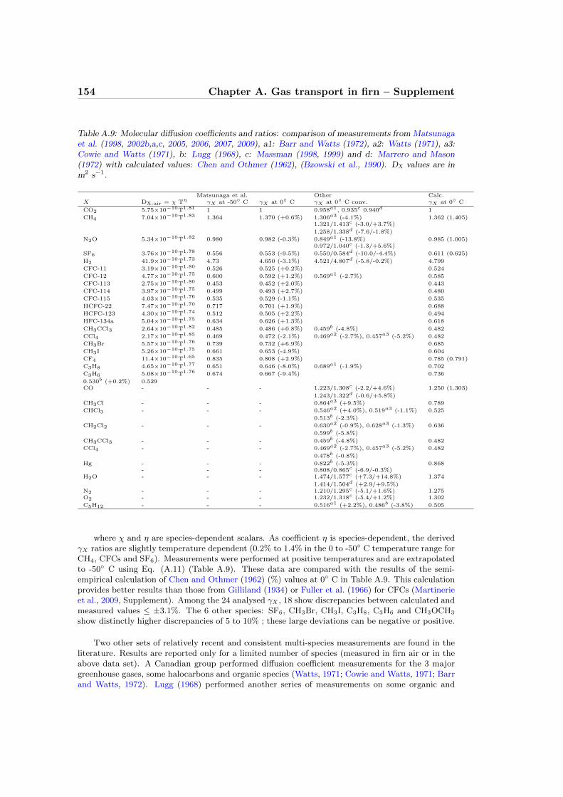
154 Chapter A. Gas transport in firn – Supplement

Table A.9: Molecular diffusion coefficients and ratios: comparison of measurements from Matsunagaet al. (1998, 2002b,a,c, 2005, 2006, 2007, 2009), a1: Barr and Watts (1972), a2: Watts (1971), a3:Cowie and Watts (1971), b: Lugg (1968), c: Massman (1998, 1999) and d: Marrero and Mason(1972) with calculated values: Chen and Othmer (1962), (Bzowski et al., 1990). DX values are inm2 s−1.

Matsunaga et al. Other Calc.X DX-air = χ Tη γX at -50◦ C γX at 0◦ C γX at 0◦ C conv. γX at 0◦ C

CO2 5.75×10−10T1.81 1 1 0.958a1, 0.935c 0.940d 1

CH4 7.04×10−10T1.83 1.364 1.370 (+0.6%) 1.306a3 (-4.1%) 1.362 (1.405)1.321/1.413c (-3.0/+3.7%)

1.258/1.338d (-7.6/-1.8%)

N2O 5.34×10−10T1.82 0.980 0.982 (-0.3%) 0.849a1 (-13.8%) 0.985 (1.005)0.972/1.040c (-1.3/+5.6%)

SF6 3.76×10−10T1.78 0.556 0.553 (-9.5%) 0.550/0.584d (-10.0/-4.4%) 0.611 (0.625)

H2 41.9×10−10T1.73 4.73 4.650 (-3.1%) 4.521/4.807d (-5.8/-0.2%) 4.799

CFC-11 3.19×10−10T1.80 0.526 0.525 (+0.2%) 0.524

CFC-12 4.77×10−10T1.75 0.600 0.592 (+1.2%) 0.569a1 (-2.7%) 0.585

CFC-113 2.75×10−10T1.80 0.453 0.452 (+2.0%) 0.443

CFC-114 3.97×10−10T1.75 0.499 0.493 (+2.7%) 0.480

CFC-115 4.03×10−10T1.76 0.535 0.529 (-1.1%) 0.535

HCFC-22 7.47×10−10T1.70 0.717 0.701 (+1.9%) 0.688

HCFC-123 4.30×10−10T1.74 0.512 0.505 (+2.2%) 0.494

HFC-134a 5.04×10−10T1.75 0.634 0.626 (+1.3%) 0.618

CH3CCl3 2.64×10−10T1.82 0.485 0.486 (+0.8%) 0.459b (-4.8%) 0.482

CCl4 2.17×10−10T1.85 0.469 0.472 (-2.1%) 0.469a2 (-2.7%), 0.457a3 (-5.2%) 0.482

CH3Br 5.57×10−10T1.76 0.739 0.732 (+6.9%) 0.685

CH3I 5.26×10−10T1.75 0.661 0.653 (-4.9%) 0.604

CF4 11.4×10−10T1.65 0.835 0.808 (+2.9%) 0.785 (0.791)

C3H8 4.65×10−10T1.77 0.651 0.646 (-8.0%) 0.689a1 (-1.9%) 0.702

C3H6 5.08×10−10T1.76 0.674 0.667 (-9.4%) 0.736

0.530b (+0.2%) 0.529CO - - - 1.223/1.308c (-2.2/+4.6%) 1.250 (1.303)

1.243/1.322d (-0.6/+5.8%)

CH3Cl - - - 0.864a3 (+9.5%) 0.789

CHCl3 - - - 0.546a2 (+4.0%), 0.519a3 (-1.1%) 0.525

0.513b (-2.3%)

CH2Cl2 - - - 0.630a2 (-0.9%), 0.628a3 (-1.3%) 0.636

0.599b (-5.8%)

CH3CCl3 - - - 0.459b (-4.8%) 0.482

CCl4 - - - 0.469a2 (-2.7%), 0.457a3 (-5.2%) 0.482

0.478b (-0.8%)

Hg - - - 0.822b (-5.3%) 0.868- - - 0.808/0.865c (-6.9/-0.3%)

H2O - - - 1.474/1.577c (+7.3/+14.8%) 1.374

1.414/1.504d (+2.9/+9.5%)N2 - - - 1.210/1.295c (-5.1/+1.6%) 1.275O2 - - - 1.232/1.318c (-5.4/+1.2%) 1.302

C5H12 - - - 0.516a1 (+2.2%), 0.486b (-3.8%) 0.505

where χ and η are species-dependent scalars. As coefficient η is species-dependent, the derivedγX ratios are slightly temperature dependent (0.2% to 1.4% in the 0 to -50◦ C temperature range forCH4, CFCs and SF6). Measurements were performed at positive temperatures and are extrapolatedto -50◦ C using Eq. (A.11) (Table A.9). These data are compared with the results of the semi-empirical calculation of Chen and Othmer (1962) (%) values at 0◦ C in Table A.9. This calculationprovides better results than those from Gilliland (1934) or Fuller et al. (1966) for CFCs (Martinerieet al., 2009, Supplement). Among the 24 analysed γX , 18 show discrepancies between calculated andmeasured values ≤ ±3.1%. The 6 other species: SF6, CH3Br, CH3I, C3H8, C3H6 and CH3OCH3

show distinctly higher discrepancies of 5 to 10% ; these large deviations can be negative or positive.

Two other sets of relatively recent and consistent multi-species measurements are found in theliterature. Results are reported only for a limited number of species (measured in firn air or in theabove data set). A Canadian group performed diffusion coefficient measurements for the 3 majorgreenhouse gases, some halocarbons and organic species (Watts, 1971; Cowie and Watts, 1971; Barrand Watts, 1972). Lugg (1968) performed another series of measurements on some organic and

A.3. Modeling firn air transport at NEEM 155

halocarbon species, as well as Mercury. Lugg (1968) did not measure D0CO2

, thus the value fromMatsunaga et al. (1998) at 25◦C is used to calculate γX in this case. Only Watts (1971) providestemperature-dependent data, other references report measurements at 25◦C. The γX in Table A.9are relative to the Matsunaga et al. (1998) data. It should be noted that D0

CO2from Matsunaga

et al. (1998) is higher than all other reported values. Deviations of the Canadian data (Watts, 1971;Cowie and Watts, 1971; Barr and Watts, 1972) from calculated values (Chen and Othmer, 1962) arevariable within the range: -13.8 to +9.5%. The differences between γX derived from Lugg (1968)and calculated values are mostly negative and range between -5.8 and +0.2%.

Table A.9 also shows γX values from two diffusion coefficient data compilations (Marrero andMason, 1972; Massman, 1998, 1999). These compilations do not include the data set by the Mat-sunaga group. As the data are generally different for the various reported chemical species, the“best” D0

CO2value to be used for the calculation of γX is unclear in the case of data compilations.

Thus both values are calculated in Table A.9 under the form X/Y, where X uses D0CO2

from Mat-sunaga et al. (1998) and Y uses D0

CO2from the data compilation. Deviations from the calculated

values (Chen and Othmer, 1962) are somewhat similar: -6.9 to +14.8% for Massman (1998, 1999),and -10.0 to +9.5% for Marrero and Mason (1972). It should be noted than for SF6, the datacompilation from Marrero and Mason (1972) is more consistent with the Matsunaga et al. (1998)value than with the calculated value.

Finally, the Chen and Othmer (1962) calculated γX are compared with the results from Bzowskiet al. (1990), shown between parentheses in the last column of Table A.9. Bzowski et al. (1990)used an elaborated calculation derived from the corresponding state theory to calculate diffusioncoefficients in equimolar mixtures of N2 and several gases. The resulting γX are always larger thatthose from Chen and Othmer (1962) (+0.8 to +4.2%) and show increased differences with the dataset by the Matsunaga group, except for CF4 (the two calculated values are very close in this case:0.8%). The Bzowski et al. (1990) calculation further increases the large discrepancy with the dataobtained for SF6 with the Chen and Othmer (1962) calculation.

A.3.1.2 Diffusion coefficients for trace gases and isotopic ratios at theNEEM site

The diffusion coefficient ratios γX for both trace gases and isotopic ratios that are used in this studyare listed in Tables A.10 and A.11. The tables also include gases that are not directly used here,but might be of interest to firn air modeling studies in general.

We would like to add a few notes on how the diffusion coefficients were derived, and how theyshould be used. First, all diffusion coefficients reported here are the binary diffusivity of the gasinto air. This satisfies the requirement, in order for Fick’s Law of diffusion to be valid, that thegas species being modeled is diffusing into a background gas that is the major gas present. In ourcontext, that major gas is air. The values are presented as ratios to the diffusivity of CO2-air. Thusthe values presented are unitless. This convention is followed even in the case of isotopic species.

Second, experimental values reported by the Matsunaga group are used where possible, extrap-olated to -28.9◦C. Where this is not possible, calculated values are given using the method of Chenand Othmer (1962). The latter are identified in Table A.10 with an asterisk (∗). Values for isotopicspecies are calculated using the “square root of the ratio of the reduced masses” law:

DX-air =

√M−1

X +M−1air

M−1Y +M−1

air

DY-air (A.12)

where X refers to the minor isotopic species, and Y to the major isotopic species. The mass Mis calculated for air by assuming that water vapor in the firn is saturated at -28.9◦C, and that themole fraction of water vapor is given by pH2O/p, where p is the barometric pressure of 745 mbar atNEEM. The saturation vapor pressure over ice is:

pH2O(mbar) = 6.1115 exp

[Θ(23.036 − Θ/333.7)

279.82 + Θ

](A.13)

156 Chapter A. Gas transport in firn – Supplement

Table A.10: Diffusion coefficients of several trace gases at the NEEM site as used in this study.T = 244.25 K, p = 745 mbar. Values are based on Matsunaga et al. (1998, 2002b,a,c, 2005, 2006,2007, 2009), unless marked with an asterisk. For those cases Eq. (A.9) is used (Chen and Othmer,1962). For all these trace gases we use the natural isotopic abundance of the constituent atomswhen calculating the molar mass.

Gas (X) γXCO2 1.000CH4 1.367N2O 0.981SF6 0.554H2 4.694CFC-11 0.525CFC-12 0.596CFC-113 0.453CFC-114 0.496CFC-115 0.532HCFC-22 0.710HCFC-123 0.509HFC-134a 0.630HFC-32 0.866HCFC-124 0.538HFC-125 0.589HFC-143a 0.647HFC-43-10mee 0.383CH3Br 0.736CH3I 0.658CF4 0.823C3H8 0.649C3H6 0.671CH3OCH3 0.827C2H5OC2H5 0.525CH3CCl3 0.485CCl4 0.470CH2Cl2 0.709@seriesCHCl3 0.595@seriesC2H5Cl 0.743@seriesCH2ClCH2Cl 0.600@seriesCH2CCl2 0.641@seriesCHClCCl2 0.583@seriesCH3Cl 0.789 ∗

CO 1.250 ∗

Hg 0.868 ∗

@seriesH2O 1.374 ∗

@seriesN2 1.275 ∗

@seriesO2 1.302 ∗

@seriesC5H12 0.505 ∗

He 4.780 ∗

Ne 2.140 ∗

Ar 1.230 ∗

Kr 0.962 ∗

Xe 0.835 ∗

A.3. Modeling firn air transport at NEEM 157

Table A.11: Diffusion coefficients for specific isotopologues. To model isotopic ratios both majorand minor abundance isotopologues are to be modeled separately. Values calculated using naturalabundance diffusion coefficients listed in Table A.10 in combination with Eq. (A.12) at T = 244.25K and p = 745 mbar.

Isotopologue (X) γX for use in

HD 3.895386 δDHH 4.693994 δD13CH4 1.340806 δ13C12CH4 1.366969 δ13CCDH3 1.340469 ∗∗ δDCH4 1.366676 ∗∗ δD14CO2 0.991368 ∗∗∗ ∆14C

CO2 1.000000 † ∆14C13CO2 0.995613 ∗∗∗ δ13C12CO2 1.000048 ∗∗∗ δ13C12C18O16O 0.991401 δ18O12C17O16O 0.995648 δ17O12C16O16O 1.000089 δ17O and δ18O12C18O 1.228754 δ18O12C17O 1.239117 δ17O12C16O 1.250172 δ17O and δ18O15N14N16O 0.976915 ‡ αδ15N, βδ15N18ON2 0.972718 δ18O17ON2 0.976884 δ17O16ON2 0.981239 αδ15N, βδ15N, δ17O,δ18O15N14N 1.263893 δ15N14N14N 1.275084 δ15N18O16O 1.283719 δ18O17O16O 1.292637 δ17O16O16O 1.302087 δ17O and δ18O22Ne 2.087122 δ22Ne and δNe/Ar20Ne 2.145608 δ22Ne40Ar 1.229952 δ40Ar38Ar 1.243488 δ38Ar36Ar 1.258324 δ40Ar, δ38Ar, Kr,Xe,Ne86Kr 0.958741 δ86Kr84Kr 0.961616 δ84Kr and δKr/Ar82Kr 0.964621 δ86Kr and δ84Kr136Xe 0.832366 δ136Xe132Xe 0.834581 δ132Xe and δXe/Ar129Xe 0.836327 δ136Xe and δ132Xe

∗∗ Includes mass effect of 13C-containing isotopologue in itsnatural abundance, in keeping with convention for reportingdeuterium data

∗∗∗ Includes mass effects of 17O- and 18O- containing isotopo-logues in their natural abundances, in keeping with conventionsfor reporting 14C and 13C data (e.g. Craig (1957),Stuiver and Polach (1977))

† Convention for reporting 14C has it as the ratio to non-isotopic (i.e. natural abundance) C

‡ This value applies to both isotopomers having the 15N at thecentral and terminal positions (Yoshida and Toyoda, 2000) .

158 Chapter A. Gas transport in firn – Supplement

where Θ is the temperature in ◦C. The mass of dry air is calculated from the 1976 US StandardAtmosphere (CRC, 2002), with a small adjustment for the increase in the mass of dry air due to aconcentration update for the anthropogenic gases (CO2 385 ppm, O2 20.9367%, N2 78.088%). Thisresults in an air mass Mair of 28.9589 g mol−1.

Third, an isotopic substitution in a gas molecule affects the diffusivity by changing the mass.The term “isotopologue” is used for a specific isotopic species. For example, 12C18O16O is anisotopologue of carbon dioxide. Therefore, each isotopologue has its own value of diffusivity intoair. To satisfy the above requirement for Fick’s Law to be valid, each isotopologue must be modeledseparately, as a trace gas diffusing into a major gas (i.e. air), each with its own diffusivity. Then, thecustomary delta value must be computed from the modeled depth profiles of the two isotopologues.For example, the δ18O value for the 12C18O16O isotopologue would be calculated from the outputsof two separate model runs, one for 12C18O16O-air and one for 12C16O16O-air:

δ18O =

([12C18O16O]model

[12C16O16O]model

/[12C18O16O]

[12C16O16O]

∣∣∣∣std

− 1

)× 103 (A.14)

where the square brackets denote a mole fraction of the isotopologue in air. The subscript‘model’ refers to mole fractions as calculated by the model, and the subscript ‘std’ refers to the ratioof mole fractions of the reference standard used for reporting the delta value (here, this would beV-PDB).

Fourth, to relate the values of diffusivities for isotopic species (i.e. species with well definedisotopic substitutions) to the values for non-isotopic species (i.e. having no specified isotopic substi-tutions and a mass corresponding to the sum of all isotopes/isotopologues, weighed by their naturalabundance) in an internally consistent way, we calculated the ratio of the diffusivity of gas Y (themajor isotopologue) to the diffusivity of the non-isotopic species NI using the equation:

DY-air

DNI-air=

√M−1

Y +M−1air

M−1NI +M−1

air

(A.15)

The mass of the non-isotopic species MNI for this purpose was the natural abundance mass (anabundance-weighted average of the masses of all the isotopes). This ratio was then multiplied bythe value of DNI/DCO2 for the non-isotopic species (typically an experimental value), to producethe final values of DY/DCO2 for the major, and DX/DCO2 for the minor isotopologue:

γY = DY/DCO2 =DY-air

DNI-air×DNI/DCO2 (A.16)

γX = DX/DCO2 =DX-air

DY-air×DY/DCO2 (A.17)

The differences between DY and DNI are not significant in most cases, but we nonethelesscalculated them for the sake of conceptual clarity. For example, the value of DY/DCO2 for theisotopologue 12C16O16O is 1.000089, compared with the value of DNI/DCO2 of 1.000000 (by defi-nition). The reason that the natural-abundance isotopic mixture diffuses slightly more slowly thanthe isotopologue 12C16O16O is that the mixture contains trace amounts of heavier isotopologuessuch as 13C16O16O.

Fifth, the non-isotopic species are generally not used to calculate delta values (∆14C is anexception). Rather, the species in the denominator in the delta calculation is generally a specificisotope, usually the major isotope, such as 1H, 12C, 14N, or 16O. Also, Table A.10 only presents threeor four significant figures for the diffusivities for non-isotopic species. This is not usually sufficientfor delta calculations. So all δ calculations should use the diffusivities in Table A.11, which have6 or 7 significant figures. Of course, the absolute values are not that well known, but the relativevalues of a pair are quite well known, as the relative values depend only on Eq. (A.12).

Sixth, the convention for reporting isotopic data usually includes all isotopologues containing acertain isotope, not just the most abundant one. For example, δ13C is defined as:

A.3. Modeling firn air transport at NEEM 159

δ13C =

(13C12C

∣∣∣∣sample

/13C12C

∣∣∣∣V-PDB

− 1

)× 103 (A.18)

For CO2, the numerator here would include the sum of the abundances of not only 13C16O16O,but also 13C17O16O, 13C18O16O, 13C18O18O, etc. The denominator would include 12C16O16O,12C17O16O, 12C18O16O, 12C18O18O, etc. Although it is impossible to measure all the minor 13C-containing isotopologues with mass spectrometry, a correction is routinely applied that approxi-mately accounts for all of these. Similarly, chemical transformations often bring all the variousforms of isotopes into a single isotopologue, as part of a routine analysis. For example, H2 gas isproduced chemically during the analysis of deuterium/hydrogen ratios in methane. For this rea-son the mass used to calculate diffusion coefficients should be a weighted average of the variousisotopologues that exist, which will ultimately contribute to the analysis.

We account for this effect in several cases, marked with asterisks. In other cases we neglect it asthe abundances are too small to be significant (for example, 13C is relatively abundant at 1 in 100carbon atoms, so we account for it, but deuterium is extremely rare at 1 in 6500 hydrogen atoms,so we neglect its effect on the weighted average mass). In still other cases we neglect it because theprecision of the measurements is far too low for this issue to matter (e.g., 15N2O).

A.3.2 Model description

Below follows a brief description of the different firn air models in alphabetical order.

A.3.2.1 CIC model

The CIC firn air model is a finite difference 1-D diffusion model coded in MATLAB. It uses implicitCrank-Nicholson time stepping to solve what is essentially an advection-diffusion-reaction equation,with radioactive decay and bubble trapping taking the place of the chemical reaction by removingtrace gas molecules from the open pore space. The model uses a stationary reference frame withz = 0 at the surface. The firn column is assumed to be isothermal and in steady state with regardto ice flow and densification rates.

The model includes four types of transport: molecular diffusion, gravitational settling, advec-tion, and eddy diffusion. The last term includes convective transport following Kawamura et al.(2006), as well as dispersive mixing in the LIZ. Using a molecular diffusivity in the LIZ insteadwould lead to continued gravitational enrichment with depth, which contradicts observations.

The transport description closely follows Trudinger et al. (1997); the main differences beinga static reference frame rather than a Lagrangian one, and the explicit inclusion of the trappingprocess in the equations of mass conservation. Advection is included through a flux in the openpores at a velocity wair:

wair =Aρice

s∗opp0

(scl(zCOD)pcl(zCOD)

ρCOD− scl(z)pcl(z)

ρ(z)

)(A.19)

where zCOD is the full close-off depth where all the air is occluded in bubbles (sop(zCOD) = 0),pcl/p0 is the pressure in closed bubbles relative to atmosphere and s∗op is the effective open porosity

s∗op = sop exp

[Mairgz

RT

](A.20)

We tune the inverse tortuosity profile τ−1(z); the effective molecular diffusivity is given asDX(z) = D0

Xτ−1(z). As an initial guess for τ−1

0 (z) we use the parameterisation by Schwander(1989). The optimal diffusivity for NEEM can be written as

τ−1(z) = τ−10 (z) × [1 + f(z)] (A.21)

where f(z) is a smooth function which we will try to estimate in the tuning procedure. Weconstruct f(z) from its Fourier components

160 Chapter A. Gas transport in firn – Supplement

f(z) = c0 +

N∑n=1

[cn sin

(nπz2L

)+ dn cos

(nπz2L

)](A.22)

where L is the total length of the open porosity firn column (78 m), and N determines thesmoothness of the final diffusivity profile. The optimal values of the coefficients cn and dn are foundin an automated gradient method. For the tuning of NEEM a value of N = 20 was used. Weset max[τ−1(z)] = 1, i.e. the diffusivity in the firn cannot exceed the free-air diffusivity. It wasfound that including other functions fi(z), such as linear slopes fi(z) = z/L, tends to speed up theconvergence to the final solution. More details will be given elsewhere.

A.3.2.2 CSIRO model

The CSIRO firn model is based on the model described by Trudinger et al. (1997). Since then it hasbeen rewritten into Fortran90, flux smoothing is no longer used, and an implicit time stepping, thesame as that used by Rommelaere et al. (1997), has replaced the Euler predictor-corrector scheme.The time step used here was 0.1 years up to 2000 then 0.01 years to the end. An exponential eddydiffusion flux has been added following Severinghaus et al. (2001) to account for convective mixingnear the surface, with 2 tuned parameters (surface magnitude and scale depth). A key differencebetween the CSIRO firn model and the other models is that it neglects the upward flux of air due tocompression of pore space. A genetic algorithm (from Haupt and Haupt (1998)) is used to calibratethe diffusivity versus open porosity and the eddy diffusion parameters. We adjust the open porosityvalues corresponding to about 12 specified diffusivity values to give the diffusivity profile, with cubicsplines used to interpolate between these points, and diffusivity capped at 500 m2 yr−1 (0.158×10−4

m2 s−1) near the surface. We only allow monotonic solutions (as defined by the points) but the cubicsplines, which match the gradient of adjacent splines at each point, can often lead to non-monotonicdiffusivity vs open porosity profiles. We therefore penalise oscillatory behaviour with an additionalterm added to the cost function that is the squared difference between a line integral following thecubic spline and a line integral for linear interpolation between the points. Any negative diffusivityvalues are set to zero. The best solution for the NEEM EU hole had the diffusivity going to zero,then increasing above zero below this. This was not intentional, but was caused by the cubic splines.The US case did not generate the same behaviour, instead the best fit was obtained with diffusivitythat decreased to zero at about 63 m. The genetic algorithm does not require an initial guess, butdoes require a range for each parameter. The ranges were initially chosen as representative of valuesfor other calibrated sites, and extended if solutions from the genetic algorithm with low values ofthe cost function collected near either end of the range. More detail on the calibration method willbe given in Trudinger et al. (in preparation).

A.3.2.3 INSTAAR model

The INSTAAR one-dimensional firn gas transport model was originally based on a model describedin Severinghaus and Battle (2006), but has evolved substantially. The model has fixed coordinateswith only the gases moving through the firn matrix. The firn matrix is considered to be in steadystate. The NEEM firn is parameterised with 1 m deep boxes between -0.5 and 59.5 m (top modelbox is half-free air, half-firn), and with 0.25 m deep boxes below 59.5 m.

Gases are moved through the firn by four mechanisms: (1) molecular diffusion (different fordifferent gases), (2) gravitational settling, (3) eddy diffusion or turbulent mixing (same for allgases), (4) downward advection (same for all gases). For each box, the model keeps track of the gascontent in the open porosity as well as in the ice-enclosed bubbles, but the gas mixing ratios areonly tracked in the open porosity part. Rate of total downward air advection is determined fromthe air content of ice below close-off and the ice accumulation rate. From mass conservation, thetotal downward air advection should be the same at each level. The rate of advection in the openporosity at each level is therefore calculated as the total downward air advection rate minus theadvection of air in the bubbles at that level (found from bubble air content and ice accumulationrate).

A.3. Modeling firn air transport at NEEM 161

Unlike the model described in Severinghaus and Battle (2006), the INSTAAR model does nothave any fundamental differences in the mechanisms of gas movement between the diffusive zoneand the lock-in zone. In the INSTAAR model the reduced gas movement in the lock-in zone isachieved simply through adjusting the overall effective gas diffusivities to lower levels.

The model includes a seasonal temperature cycle and calculates firn temperature in each modelbox in the same way as the Severinghaus and Battle (2006) firn model.

The model uses explicit time stepping. To avoid computational instability the time step isalways chosen to be smaller than ∆t < (∆z)2/3Dtotal, where ∆t is the time step, ∆z is the box sizein m, and Dtotal is the total effective diffusivity in m2 s−1. For all gases except H2, this time stepwas set to 11,119 s (3.5× 10−4 yr). For H2, which has a much higher molecular diffusivity, the timestep was set to 3,156 s (1 × 10−4 yr).

The equation used to calculate flux of gas X between two adjacent boxes due to moleculardiffusion and gravity at each time step is as follows:

JX;molec-grav(i) = −γXD0CO2

τ−1i sop; mid ×(

Ci+1 − Ci∆zmid

− ∆Mg

RTi

Ci+1 + Ci2

)(A.23)

Here JX;molec-grav(i) is the gas flux between box i and i + 1 (in units of e.g., ppm m s−1). Thiscan be thought of as the volume of the pure gas moving across a unit area of the boundary betweenboxes per unit time. γXD

0CO2

is the free-air diffusivity of gas X at the boundary between box iand i+ 1 in m2 s−1, re-calculated at each time step to take into account firn temperature variations;τ−1i is the tuned dimensionless multiplier (or inverse tortuosity) to the free air diffusivity for boxi. sop; mid is the open porosity (m3/m3) at the boundary between the two boxes. This is includedbecause the flux should be proportional to the open porosity. Ci is the gas mixing ratio in box i(e.g., in ppm), ∆zmid is the distance (m) between the middles of box i and box i + 1, ∆M is themolar mass difference (kg mol−1) between the gas and bulk air, g is the acceleration due to gravity(m s−2), R is the universal gas constant (J mol−1 K−1) and Ti is the firn temperature (K) at theboundary between boxes i and i+ 1.

The basic form of the equation used to calculate the gas flux due to eddy diffusion or turbulentmixing is:

Jeddy(i) = −Deddy(i)sop; midCi+1 − Ci

∆zmid(A.24)

where Jeddy(i) is the gas flux due to eddy diffusion (ppm m3 m−2 s−1) and Deddy(i) is the tunededdy diffusivity (m2s−1) for box i.

Gas fluxes due to advection and flux of air into newly formed bubbles are also calculated at eachtime step. All of these fluxes are corrected to STP volumes (to account for varying temperatureand pressure in the firn column) and are added to find the total flux of gas into the box (Jin) andthe total flux of gas out of the box (Jout). The time derivative of the gas mixing ratio in box i isthen calculated as:

∆Ci∆t

=

(Jin − Jout

sop(i)∆zi

)(A.25)

where si is the open porosity in the box and ∆zi is the vertical length of box i.

The effective diffusivities in the INSTAAR model were manually tuned to optimise the fit to thesuite of 10 gases. The initial guess for effective molecular diffusivities used the free-air diffusivity inthe surface box, with effective diffusivities for CO2 declining linearly to 2.0 × 10−9 m2 s−1 at 64mand staying constant beyond 64 m. The initial guess for eddy diffusivity set the eddy diffusivityequal to molecular diffusivity for CO2 in the surface box, and prescribed an exponential decreasewith depth using an e-folding depth of 4 m. Below the depth where eddy diffusivity dropped to1.0 × 10−8 m2 s−1 it was held constant at this value.

162 Chapter A. Gas transport in firn – Supplement

A.3.2.4 LGGE-GIPSA model

In the LGGE-GIPSA model (Witrant et al., 2011), the transport processes described in (Rommelaereet al., 1997) have been revised in a poromechanics framework, where the ice lattice, the gases inopen pores and the gases in closed pores are considered as an interconnected network constrainedby mass conservation. The model dynamics is expressed in terms of densities and the diffusionprocess is described as a combination of Fick’s and Darcy’s transport, thus allowing to distinguishbetween a purely diffusive transport (molecular and eddy) in the convective layer and an almost-stagnant transport in the lower zones. The numerical implementation is done with an implicit timediscretization with a one week step and combined central/Lax-Wendroff space discretization with astep of 0.2 m.

Firn diffusivity is calculated using a constrained non linear least square multi-gas optimizationscheme, with the optimisation problem formulated by Witrant and Martinerie (2010). δ15N2 wasnot used for diffusivity optimisation but kept for the physical model transport validation. Bycontrast with some of the other models in this intercomparison, only molecular diffusivity (no eddy-diffusivity) is considered in the deep firn. An eddy diffusion term (Deddy) is taken into account inthe upper firn to represent convective transport: when firn diffusivity calculated by our optimisationprocedure exceeds the speed of molecular diffusion in free air D0

X corrected by a factor α to takeinto account the porosity effect (Severinghaus and Battle, 2006), the firn diffusivity is calculated asαD0

X +Deddy. Deddy is then the quantity tuned by our least square multi-gas optimisation in orderto best fit the firn data. No pre-defined depths are used to constrain the limits of the convective andlock-in zone except for the depth at which gravitational fractionation starts (set as 4 m for NEEM).The lower boundary for gravitational fractionation (lock-in depth) is calculated by the model.

The model has been evaluated on 12 additional Arctic (Devon Island, North GRIP, Summit)and Antarctic (DE08, Berkner Island, Siple Dome, Dronning Maud Land, South Pole 1995, SouthPole 2001, Dome C, Vostok) previously simulated with the Rommelaere et al. (1997) model.

A.3.2.5 OSU model

The OSU firn air model is a finite-difference diffusion model based on the mixing ratio equations ofTrudinger et al. (1997), Eqs. (A9) and (A13). However, the OSU model differs from this model inthe following ways. First, an eddy-diffusion term is added to represent surface convection, based onthe parameterisation of Kawamura et al. (2006), and also to account for the necessary mixing thatis observed within the LIZ but cannot be due to molecular diffusion.

Second, the model uses an implicit Crank-Nicholson numerical scheme, which makes it stableover a large range of depth increments and time steps. Because of this, at the model time step of0.005 years and depth resolution of 0.1 m, the flux smoothing technique of Trudinger et al. (1997)is not employed.

Lastly, vertical advection of the firn is accounted for by shuffling boxes down at every timestep, rather than moving the reference frame (Schwander et al., 1993). An evenly spaced depthscale is used, which makes computation of the diffusion equation simpler but complicates shiftingboxes as the firn densifies and the equally spaced boxes contain less and less air. To deal with this,the vertical displacement of the air at every depth and every time step is calculated. The verticalair velocity used to compute displacement differs from the ice velocity (Rommelaere et al., 1997)and is given by the equation of Buizert (Eq. (A.19)). This creates a new mixing-ratio profile withdifferent depth values which is then interpolated back onto the fixed grid, and assigned the correctfirn properties at each depth. The value of the top box is set to the atmospheric mixing ratio forthe current time step during this process.

Bubble compression is accounted for only in the LIZ, because above this zone it is assumedthat the pressure in the open porosity is equal to atmospheric pressure. Below the top of the LIZ,the model uses the following correction to account for the greater amount of air in the open porousvolume:

A.3. Modeling firn air transport at NEEM 163

Table A.12: Constants used in the OSU diffusivity tuning for the EU borehole

constant value unit

g1 - 0.209g2 1.515g3 0.53g4 3.17 ×10−10 m2s−1

g5 1.82 mg6 3.17 ×10−9 m2s−1

g7 0.11 m

s∗op(z) = sop(z)ρ(z)

ρLID(A.26)

where sop(z) is the true open porosity at depth z (Eq. (A.2)), ρ(z) is the density (Eq. (A.1)),and ρLID is the density at the lock-in depth, i.e. at the top of the LIZ. Bubble compression ofthe closed porosity is ignored since this is an open porosity model. The free air diffusivity of CO2

(D0CO2

= 1 × 10−5 m2 s−1) is first corrected for site temperature and pressure (Schwander et al.,1988), then adjusted for depth based on the porosity (note that this is based on the actual porosity,not the effective porosity defined above). The diffusivity parameterisation of Schwander et al. (1993)is used as a first estimate, but a second-order porosity dependence was added later to improve thefit. The form of the final diffusivity profile is:

DX(z) = D0X

[g1 + g2sop(z) + g3s

2op(z)

](A.27)

Values for constants g1, g2 and g3 were manually adjusted to minimise the total root meansquared error of the model-data mismatch for all tracers, including δ15N. Final values are listedin Table A.12. Where molecular diffusivity goes to zero in the LIZ, the model uses a syntheticexponential decrease to prevent numerical instabilities. This takes the form:

DX(z) = g4 + (DX(zLID) − g4)e−g5(z−zLID), for z > zLID (A.28)

where g4 is some relict molecular diffusivity and zLID is the lock-in depth. Dispersive eddydiffusivity in the lock-in zone is parameterised by the following exponential:

Deddy(z) = g6eg7(z−zLID), for z > zLID (A.29)

where again g6 and g7 were iteratively adjusted to provide the best fit to the data.

A.3.2.6 SIO model

The Scripps Institution of Oceanography (SIO) firn air model follows generally those of Schwanderet al. (1993), Rommelaere et al. (1997), Severinghaus and Battle (2006), and Severinghaus et al.(2010) (hereafter S2010). Slight differences from the model of S2010 include the following. (i) Baro-metric pressure increases with depth, according to the isothermal barometric equation set with theinitial mean-annual temperature, (ii) gravity is set to zero within the lock-in zone, (iii) molecularand eddy diffusion both continue throughout the LIZ, and (iv) the LIZ grid spacing is calculatedwith the air advection velocity until the close-off density (Martinerie et al., 1992) and thereafterwith the firn velocity, whereas S2010 calculated it with the firn velocity in the entire LIZ.

The main differences between the SIO model and the other models in the present intercompar-ison are:

1) The model has a parallel heat transport model within it that predicts temperature as afunction of depth and time. Using these temperatures, the model computes fractionation of gases andisotopes by thermal diffusion, gravitational settling, and temperature-sensitive kinetic disequilibrium

164 Chapter A. Gas transport in firn – Supplement

0 10 20 30 40 50 60 70

320

340

360

380

CICCSIROINSTAARLGGE−GIPSAOSUSIO

LIZDZ0 10 20 30 40 50 60 70

1200

1400

1600

1800

Depth (m)

0 10 20 30 40 50 60 70

0

1

2

3

4

5

6

7

LIZDZ0 10 20 30 40 50 60 70

0

0.05

0.1

0.15

0.2

0.25

0.3

Depth (m)

CO

2 (pp

m)

CH

4 (pp

b)

SF

6 (pp

t)δ15

N2 (

‰)

a

b

c

d

Figure A.5: (a–d) Modeled profiles for all 4 tracers from the US borehole. With the exception of(d) data have been gravity corrected and the models are run with gravity turned off. Errorbarscorrespond to full 1σ uncertainty as defined in Sect. A.2.7.

processes. Disequilibrium arises from convection in the near-surface layers, downward advectiondue to snow accumulation and bubble close-off, and transients in atmospheric gas mixing ratios andtemperatures. For the NEEM intercomparison runs, the temperature model was disabled, but thefull model was used to make thermal diffusion corrections to NEEM firn air δ15N and δ86Kr dataused as inputs.

2) The SIO model treats downward air advection in the LIZ by shifting concentrations down byone grid point every 0.5 yr, rather than with explicit advection schemes. The grid points are spacedapart by distances such that the air advection velocity wair would transport the air that distancein 0.5 yr. This scheme minimizes the numerical diffusion common to upwind advection schemes.As a result, the SIO model has the highest mixing ratio of tracer (oldest gas) in its lock-in zone inDiagnostic Test 4. This lack of numerical diffusion also implies that the diffusivities found by tuningto observed gas profiles should be slightly higher than those of the other models. This lock-in zonearchitecture was chosen so that second derivatives of atmospheric variations in trace gases would bepreserved within the lock-in zone to the extent possible. For example, the dip in atmospheric CO2

in the early 1940s can be preserved by the SIO model given a sufficiently high accumulation rate.The diffusion correction for 13CO2 and 13CH4 is also arguably more accurate with a minimum ofnumerical diffusion.

The inverse tortuosity profile τ−1(z) is tuned using a generalised least square method. The initialguess τ−1

o (z) is the parameterisation by Schwander (1989). Subsequent profiles are determined using:

A.3. Modeling firn air transport at NEEM 165

−4 −2 0 2 4

0

5

10

15CIC RMSD= 0.68

Cou

nts

−4 −2 0 2 4

0

5

10

15CSIRO RMSD= 1.06

Cou

nts

0

5

10

15INSTAAR RMSD= 0.60

Cou

nts

−4 −2 0 2 40

5

10

15LGGE−GIPSARMSD= 0.61

Cou

nts

(Model−data) / σ

−4 −2 0 2 40

5

10

15OSU RMSD= 0.75

(Model−data) / σ

Cou

nts

−4 −2 0 2 40

5

10

15SIO RMSD= 0.86

(Model−data) / σ

Cou

nts

a b

c d

e f

Figure A.6: (a–f) Histogram of (mi − di)/σi for the firn air transport models in this study usingthe US borehole data. The black curve gives a Gaussian distribution of width σ = 1, normalised tohave equal surface to the histogram. The RMSD is calculated with Eq. (3) of the main article.

τ−1(z) = τ−1o (z) +

N∑i=1

hi ∗ fi(z) (A.30)

fi(z) = 0 z < i∆z

fi(z) = a(z − i∆z)/∆z i∆z < z < (i+ 1)∆z

fi(z) = a((i+ 2)∆z − z)/∆z (i+ 1)∆z < z < (i+ 2)∆z

fi(z) = 0 z > (i+ 2)∆z

We use an amplitude a = 10−6 m2 s−1 between 0 and 60m, and a = 10−8 m2 s−1 between 60and 80m. The half width ∆z was set to ∆z = 0.5 m. The coefficients hi are optimised using a leastsquare regression to minimise the RMS misfit given in Eq. (3) of the main text.

Near the surface, the eddy diffusivity due to wind pumping is parameterised by an exponential:

Deddy(z) = D0eddy exp

(− z

H

)(A.31)

D0eddy = 1.6e−5 m2 s−1 and H = 5 m are tuned to fit the δ15N and δ86Kr data, corrected for

thermal fractionation.

166 Chapter A. Gas transport in firn – Supplement

LIZDZ0 10 20 30 40 50 60 70

0

0.5

1

1.5

10−9

10−8

10−7

10−6

10−5

CICCSIROINSTAARLGGE−GIPSAOSUSIO

0 10 20 30 40 50 60 70

0

0.2

0.4

0.6

0.8

1

Depth (m)

a

b

c

DC

O2 (

10−

5 m2 /s

)D

tota

l (m

2 /s)

Ded

dy /

Dto

tal

Figure A.7: (a) CO2 molecular diffusivity profile with depth DCO2(z) for the US borehole. (b) Semi-log plot of the total CO2 diffusivity profile Dtotal(z) = DCO2(z)+Deddy. (c) Plot of Deddy(z)/Dtotal(z).The eddy diffusion near the surface corresponds to the convective mixing, in the LIZ some of themodels have included dispersive mixing.

In the lock in zone, the balance between molecular diffusion (affecting each gas differently) anddispersion (affecting all the gases proportionally) is determined by a single coefficient α varyingbetween 0 and 1, rather than by having a free dispersion diffusivity profile, which is largely under-constrained. The molecular diffusivity is then:

DX(z) = (1 − α)D0X

τ(z)(A.32)

And the dispersion, included as an eddy diffusivity, is:

Deddy(z) = αD0

CO2

τ(z)(A.33)

Here D0CO2

is used as the reference, all gases experience the same Deddy(z). The optimum αwas αEU = 0.27 for the EU hole, and αUS = 0.35 for the US hole.

A.4. Model intercomparison and discussion 167

1980 1985 1990 1995 2000 2005 20100

5

10

15

Year

z = 63 mCIC

CSIROINSTAARLGGE−GIPSAOSUSIO

1900 1920 1940 1960 19800

1

2

3

4

Year

z = 76 m

Den

sity

( ×

10−

2 yr−

1 )D

ensi

ty (

×10

−2 y

r−1 )

a

b

Figure A.8: US borehole modeled age distribution densities for (a) z = 63m (lock-in depth) and(b) z = 76m (deepest sample). On the horizontal axis are calendar years C.E.; decimal samplingyear is 2008.54 (i.e. mid July). Age distributions are generated by applying a surface forcing whichis unity for 0.2 ≤ t < 0.4 yr, and zero elsewhere.

A.3.3 Fit of modeled profiles to the data

The firn models were tuned separately to the US borehole, for which we have firn air data for fourdifferent tracers: CO2, CH4, SF6 and δ15N2. The fit to the data is shown in Fig. A.5. As for theEU borehole we find a mismatch at depths z > 70m for CO2 (Fig. A.5A); the feature is reproducedconsistently by all the firn air models.

To assess model performance we make a histogram of (mi − di)/σi, where the index i goesover all the 77 data points of the US borehole. This is shown in Fig. A.6 together with a Gaussiandistribution of width σ = 1 and a surface area equal to that of the histogram. The figure furthermoreshows the root mean square deviation (RMSD) from the data as given by Eq. (3) of the main text.Most models perform better for the US borehole in terms of the RMSD, which is due to the factthat there are fewer tracers for the US borehole. The exception is the CSIRO model for which theRMSD is higher on the US hole. However, preliminary tests show that by including the advectiveback flux in the CSIRO model the RMSD improves to 0.79 (Trudinger et al., 2011).

168 Chapter A. Gas transport in firn – Supplement

Table A.13: Mean age, median age, Full Width at Half Maximum and Spectral Width (∆, Eq. (1)in Trudinger et al., 2002) at the lock-in depth (z = 63 m) and bottom of the LIZ (z = 76 m) forthe US borehole. All values given in years. We use the 2σ standard deviation divided by the mean(2σ/µ) as a measure of the spread in model results.

Model Mean Median FWHM ∆

z = 63 m

CIC 8.3 6.7 7.2 4.0CSIRO 7.3 6.1 6.4 3.1INSTAAR 7.7 6.2 6.6 3.7LGGE-GIPSA 12.2 8.2 8.5 8.3OSU 8.2 6.6 7.1 4.0SIO 8.1 6.5 7.0 3.92σ/µ 0.41 0.23 0.21 0.84

z = 76 m

CIC 61.6 58.1 39.8 14.6CSIRO 60.2 59.1 6.4 3.1INSTAAR 63.5 60.5 39.8 14.0LGGE-GIPSA 68.8 66.2 34.6 12.3OSU 62.1 58.9 40.3 14.2SIO 62.5 59.0 41.5 14.82σ/µ 0.09 0.10 0.81 0.74

A.4 Model intercomparison and discussion

A.4.1 Diffusivity profiles

Figure A.7a shows the reconstructed molecular diffusivity profiles for CO2 for the different modelson the US borehole. Upon reaching the LIZ the effective molecular diffusion nearly vanishes. InFig. A.7b the total diffusivity Dtotal(z) = DCO2(z) + Deddy for CO2 is plotted on a semilog scale.As for the EU borehole we observe that the models require a non-vanishing diffusivity within theLIZ to fit the data. Only the CSIRO model uses zero diffusivity in the LIZ for the US hole. Thisdifference might explain why the CSIRO model has more difficulty fitting the US data, as expressedby the RMSD in Fig. A.6.

A.4.2 Gas age distributions

Figure A.8 compares age distribution densities for the models at the lock-in depth (z = 63 m) andnear the deepest sample (z = 76 m) on the US hole. Table A.13 gives some characteristics of thedistributions. On the EU hole we find a spread of up to 25% in the mean ages and distributionwidths at 63 m depth. When looking at the US hole the spread in the calculated mean ages is evenlarger (40% of the mean age at 63 m). This large spread is mostly due to the LGGE-GIPSA model,which stands out as having a wider and flatter age distribution. However, since this model obtainsa better fit to the experimental data than most models (Fig. A.6) this distribution is certainlyrealistic. We attribute the larger spread found in modeled US borehole mean ages to the fact that ithas fewer tracers. This leaves the mean age more poorly constrained. The CSIRO age distributionat z = 76 m is very narrow compared to the other models, due to the absence of LIZ diffusion inthe US hole. Since it differs so strongly from both the CSIRO model result on the EU hole, aswell as from the other model results on the US hole, this age distribution was not included in thecomparison in Fig. 7 of the main article.

A.4. Model intercomparison and discussion 169

0 10 20 30 40 50 60 70

−0.12

−0.1

−0.08

−0.06

−0.04

−0.02

0

CICCSIROINSTAARLGGE−GIPSAOSUSIO

0 10 20 30 40 50 60 70

10−4

10−3

10−2

10−1

100

LIZDZ0 10 20 30 40 50 60 70

0

0.05

0.1

0.15

0.2

0.25

0.3

Depth (m)

LIZDZ0 10 20 30 40 50 60 70

0

200

400

600

800

Depth (m)

δ13C

O2 (

‰)

δ grav

(‰

)

Am

plitu

de |c

|A

ge o

f air

(yrs

)

a b

c d

Figure A.9: Model comparison using the four diagnostic scenarios and diffusivity tuned to the USborehole data. (a) Scenario I: Diffusive fractionation for a hypothetical monotonic CO2 increase.(b) Scenario II: Attenuation of a 15 yr period sinusoidal CO2 forcing with depth. (c) ScenarioIII: Gravitational enrichment for gas X with D0

X = 0.025D0CO2. Data points show gravitational

enrichment of 15N2 corrected for the effect of thermal diffusion. (d) Scenario IV: Mean age of gasY , using advective transport only (D0

Y = 0). With the exception of S-III all scenarios were run withthe effect of gravity turned off.

A.4.4 Synthetic diagnostic scenarios

Table A.14 provides detailed specifications on how the diagnostic scenarios are run in the models.

Scenario I compares the amount of diffusive fractionation (DF) of isotopes in the firn. We modelthe mole fractions of [12CO2] and [13CO2] separately using the relative diffusion coefficients givenin Sect. A.3.1.2. For convenience we let our reference atmosphere have the property

13Rstd =[13CO2]

[12CO2]

∣∣∣∣std

= 1 (A.34)

meaning that at in the atmosphere [12CO2] = [13CO2] as we let the mixing ratio increase withtime. We use the same atmospheric input file to force both isotopologues. The fractionation withdepth is then given as

δ13CO2(z) =

([13CO2](z)

[12CO2](z)− 1

)× 103 h (A.35)

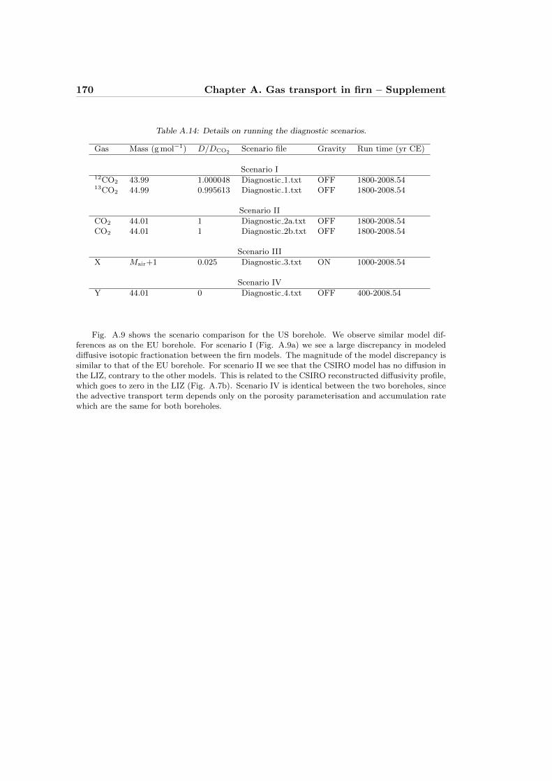
170 Chapter A. Gas transport in firn – Supplement

Table A.14: Details on running the diagnostic scenarios.

Gas Mass (g mol−1) D/DCO2 Scenario file Gravity Run time (yr CE)

Scenario I12CO2 43.99 1.000048 Diagnostic 1.txt OFF 1800-2008.5413CO2 44.99 0.995613 Diagnostic 1.txt OFF 1800-2008.54

Scenario II

CO2 44.01 1 Diagnostic 2a.txt OFF 1800-2008.54CO2 44.01 1 Diagnostic 2b.txt OFF 1800-2008.54

Scenario III

X Mair+1 0.025 Diagnostic 3.txt ON 1000-2008.54

Scenario IV

Y 44.01 0 Diagnostic 4.txt OFF 400-2008.54

Fig. A.9 shows the scenario comparison for the US borehole. We observe similar model dif-ferences as on the EU borehole. For scenario I (Fig. A.9a) we see a large discrepancy in modeleddiffusive isotopic fractionation between the firn models. The magnitude of the model discrepancy issimilar to that of the EU borehole. For scenario II we see that the CSIRO model has no diffusion inthe LIZ, contrary to the other models. This is related to the CSIRO reconstructed diffusivity profile,which goes to zero in the LIZ (Fig. A.7b). Scenario IV is identical between the two boreholes, sincethe advective transport term depends only on the porosity parameterisation and accumulation ratewhich are the same for both boreholes.

A.4. Model intercomparison and discussion 171

Notation

A Accumulation rate (m yr−1 ice equivalent)Aabs Absolute 14C abundance (1.1764 × 10−12)C Mixing ratio (mol mol−1)Deddy Eddy diffusion coefficient (m2 s−2)DX Diffusion coefficient of gas X (m2 s−2)D0X Free air diffusion coeff. of gas X (m2 s−2)

di Data point ig Gravitational acceleration (9.82 m s−2)J Trace gas flux (mol mol−1 m s−1)Mair Molar mass of air (kg mol−1)MX Molar mass of gas X (kg mol−1)mi Modeled value for data point ip Air pressure (Pa)pH2O Vapour pressure of water (Pa)R Molar gas constant (8.314 J mol−1 K−1)RMSD Root Mean Square Deviations Total porosity (m3 m−3)sco Mean close-off porosity (m3 m−3)sop(cl) Open (closed) porosity (m3 m−3)s∗op Effective open porosity (m3 m−3)T Absolute temperature (K)uX Uncertainty in gas X (mol mol−1)Vcontam/V Fraction of contamination (m3 m−3)wair Downward velocity of air (m s−1)wice Downward velocity of ice layers (m s−1)[X] Mixing ratio of gas X (mol mol−1)xair Air content of ice (mL STP per kg ice)z Depth (m)zCOD Full close-off depth; sop(zCOD) = 0 (m)zLID Lock-in depth (m)γX Diffusion coefficient relative to CO2

∆age Ice age-gas age difference (yr)∆ageop Ice age- open pore gas age difference (yr)∆M Molar mass deviation from air (kg mol−1)∆t Temporal step size (s) or (yr)∆z Spatial step size (m)δgrav Gravitational fractionation p. unit mass (h)Θ Temperature (◦ C)θ Trapping rate (s−1)λX Radioactive decay constant of gas X (s−1)µ Mean value of a seriesρ Firn density (g cm−3)ρco Mean close-off density (g cm−3)ρCOD Full close-off density; ρ(zCOD) (g cm−3)ρice Solid ice density (g cm−3)σi Assigned uncertainty for data point iτ Tortuosityτ0 Initial guess for τ in tuning algorithmφop(cl) Air flux in open (closed) porosity (m s−1)

172 Chapter A. Gas transport in firn – Supplement

A.5 References

Arnaud, L., Barnola, J. M., and Duval, P. (2000). Physical modeling of the densification of snow/firnand ice in the upper part of polar ice sheets. In Hondoh, T., editor, Physics of Ice Core Records,pages 285–305. Hokkaido University Press.

Aydin, M., Montzka, S. A., Battle, M. O., Williams, M. B., De Bruyn, W. J., Butler, J. H., Verhulst,K. R., Tatum, C., Gun, B. K., Plotkin, D. A., Hall, B. D., and Saltzman, E. S. (2010). Post-coring entrapment of modern air in some shallow ice cores collected near the firn-ice transition:evidence from cfc-12 measurements in antarctic firn air and ice cores. Atmos. Chem. Phys.,10(11):5135–5144.

Barr, R. F. and Watts, H. (1972). Diffusion of some organic and inorganic compounds in air. J.Chem. Eng. Data, 17(1):45–46.

Blanc, A. (1908). Recherches sur les mobilites des ions dans les gaz. J. Phys. Theor. Appl., 7:825–839.Buizert, C., Martinerie, P., Petrenko, V. V., Severinghaus, J. P., Trudinger, C. M., Witrant, E.,

Rosen, J. L., Orsi, A. J., Rubino, M., Etheridge, D. M., Steele, L. P., Hogan, C., Laube, J. C.,Sturges, W. T., Levchenko, V. A., Smith, A. M., Levin, I., Conway, T. J., Dlugokencky, E. J.,Lang, P. M., Kawamura, K., Jenk, T. M., White, J. W. C., Sowers, T., Schwander, J., and Blunier,T. (2011). Gas transport in firn: multiple-tracer characterisation and model intercomparison forneem, northern greenland. Atmos. Chem. Phys. Discuss., 11:15975–16021.

Bzowski, J., Kestin, J., Mason, E. A., and Uribe, F. (1990). Equilibrium and transport propertiesof gas mixtures at low density: eleven polyatomic gases and five noble gases. J. Phys. Chem. Ref.Data, 19:1179–1232.

Chen, N. H. and Othmer, D. F. (1962). New generalized equation for gas diffusion coefficient. J.Chem. Eng. Data, 7(1):37–41.

Cowie, M. and Watts, H. (1971). Diffusion of methane and chloromethanes in air. Can. J. Chem.,49:74–77.

Craig, H. (1957). Isotopic standards for carbon and oxygen and correction factors for mass-spectrometric analysis of carbon dioxide. Geochim. Cosmochim. Ac., 12(1-2):133 – 149.

CRC (2002). CRC Handbook of Chemistry and Physics, 83rd Edition. CRC Press, Boca Raton, FL,USA.

Etheridge, D., Steele, L., Francey, R., and Langenfelds, R. (1998). Atmospheric methane between1000 AD and present: Evidence of anthropogenic emissions and climatic variability. J. Geophys.Res.-Atm., 103(D13):15979–15993.

Etheridge, D. M., Steele, L. P., Langenfelds, R. L., Francey, R. J., Barnola, J. M., and Morgan, V. I.(1996). Natural and anthropogenic changes in atmospheric co2 over the last 1000 years from airin antarctic ice and firn. J. Geophys. Res., 101(D2):4115–4128.

Fink, D., Hotchkis, M., Hua, Q., Jacobsen, G., Smith, A., Zoppi, U., Child, D., Mifsud, C., van derGaast, H., Williams, A., and Williams, M. (2004). The ANTARES AMS facility at ANSTO.Nucl. Instrum. Meth. B, 223:109–115.

Francey, R., Allison, C., Etheridge, D., Trudinger, C., Enting, I., Leuenberger, M., Langenfelds, R.,Michel, E., and Steele, L. (1999). A 1000-year high precision record of delta C-13 in atmosphericCO2. Tellus B, 51(2):170–193.

Fuller, E. N., Schettler, P. D., and Giddings, J. C. (1966). A new method for prediction of binarygas-phase diffusion coefficients. Ind. Eng. Chem., 58:19–27.

Gilliland, E. R. (1934). Diffusion coefficients in gaseous systems. Ind. Engng. Chem., 26:681–685.Goujon, C., Barnola, J. M., and Ritz, C. (2003). Modeling the densification of polar firn including

heat diffusion: Application to close-off characteristics and gas isotopic fractionation for Antarcticaand Greenland sites. J. Geophys. Res.-Atm, 108(D24):18.

Guzman, M. I., Hoffmann, M. R., and Colussi, A. J. (2007). Photolysis of pyruvic acid in ice:Possible relevance to co and co2 ice core record anomalies. J. Geophys. Res.-Atm, 112(D10):10.

Haupt, R. L. and Haupt, S. E. (1998). Practical Genetic Algorithms. John Wiley & Sons, Inc.,Hoboken, New Jersey.

Hua, Q. and Barbetti, M. (2004). Review of tropospheric bomb C-14 data for carbon cycle modelingand age calibration purposes. Radiocarbon, 46(3):1273–1298.

A.5. References 173

Karlen, I., Olsson, I. U., Kallburg, P., and Kilici, S. (1968). Absolute determination of the activityof two 14c dating standards. Arkiv Geofysik, 4:465–471.

Kawamura, K., Severinghaus, J. P., Ishidoya, S., Sugawara, S., Hashida, G., Motoyama, H., Fujii,Y., Aoki, S., and Nakazawa, T. (2006). Convective mixing of air in firn at four polar sites. EarthPlanet Sc. Lett., 244(3-4):672–682.

Lal, D., Jull, A. J. T., Donahue, D. J., Burtner, D., and Nishiizumi, K. (1990). Polar ice ablationrates measured using in-situ cosmogenic c-14. Nature, 346(6282):350–352.

Levin, I., Hammer, S., Kromer, B., and Meinhardt, F. (2008). Radiocarbon observations in at-mospheric CO2: Determining fossil fuel CO2 over Europe using Jungfraujoch observations asbackground. Sci. Total Environ., 391(2-3):211–216.

Levin, I. and Kromer, B. (2004). The tropospheric (CO2)-C-14 level in mid-latitudes of the NorthernHemisphere (1959-2003). Radiocarbon, 46(3):1261–1272.

Levin, I., Naegler, T., Heinz, R., Osusko, D., Cuevas, E., Engel, A., Ilmberger, J., Langenfelds,R. L., Neininger, B., Rohden, C. v., Steele, L. P., Weller, R., Worthy, D. E., and Zimov, S. A.(2010a). The global sf6 source inferred from long-term high precision atmospheric measurementsand its comparison with emission inventories. Atmos. Chem. Phys., 10(6):2655–2662.

Levin, I., Naegler, T., Kromer, B., Diehl, M., Francey, R. J., Gomez-Pelaez, A. J., Steele, L. P.,Wagenbach, D., Weller, R., and Worthy, D. E. (2010b). Observations and modelling of the globaldistribution and long-term trend of atmospheric (CO2)-C-14. Tellus B, 62(3):207.

Lugg, G. A. (1968). Diffusion coefficients of some organic and other vapors in air. Anal. Chem.,40:1072–1077.

Manning, M. and Melhuish, W. H. (1994). Atmospheric delta 14c record from wellington. In Trends:A Compendium of Data on Global Change. Carbon Dioxide Information Analysis Center, OakRidge National Laboratory, U.S. Department of Energy, Oak Ridge, Tenn., U.S.A.

Marrero, T. R. and Mason, E. A. (1972). Gaseous diffusion coefficients. J. Phys. Chem. Ref. Data,1:3–118.

Martinerie, P., Lipenkov, V. Y., Raynaud, D., Chappellaz, J., Barkov, N. I., and Lorius, C. (1994).Air content paleo record in the vostok ice core (antarctica): A mixed record of climatic andglaciological parameters. J. Geophys. Res., 99:10565–10576.

Martinerie, P., Nourtier-Mazauric, E., Barnola, J. M., Sturges, W. T., Worton, D. R., Atlas, E.,Gohar, L. K., Shine, K. P., and Brasseur, G. P. (2009). Long-lived halocarbon trends and budgetsfrom atmospheric chemistry modelling constrained with measurements in polar firn. Atmos.Chem. Phys., 9(12):3911–3934.

Martinerie, P., Raynaud, D., Etheridge, D. M., Barnola, J. M., and Mazaudier, D. (1992). Physicaland climatic parameters which influence the air content in polar ice. Earth Planet Sc. Lett.,112(1-4):1–13.

Massman, W. J. (1998). A review of the molecular diffusivities of h2o, co2, ch4, co, o3, so2, nh3,n2o, no, and no2 in air, o2 and n2 near stp. Atmos. Environ., 32:1111–1127.

Massman, W. J. (1999). Molecular diffusivities of hg vapor in air, o2 and n2 near stp and and thekinematic viscosity and thermal diffusivity of air near stp. Atmos. Environ., 33:453–457.

Matsunaga, N., Hori, M., and Nagashima, A. (1993). Mutual diffusion coefficients of halogenated-hydrocarbon refrigerant-air systems. High Temp.-High Press., 25:185–192.

Matsunaga, N., Hori, M., and Nagashima, A. (1998). Diffusion coefficients of global warming gasesinto air and its component gases. High Temp.-High Press., 30(1):77–83.

Matsunaga, N., Hori, M., and Nagashima, A. (2002a). Measurements of mutual diffusion coefficientsgases by the taylor method: measurements on h2-air, h2-n2, and h2-o2 sustems. Heat Trans. AsianRes., 31:182–193.

Matsunaga, N., Hori, M., and Nagashima, A. (2002b). Measurements of the mutual diffusioncoefficients of gases by the taylor method (7th report, measurements on the sf6-air, sf6-n2, sf6-o2,cfc12-n2, cfc12-o2, hcfc22-n2 and hcfc22-o2 systems). Trans. Jpn. Soc. Mech. Eng. B., 68:550–555.

Matsunaga, N., Hori, M., and Nagashima, A. (2002c). Measurements of the mutual diffusion coef-ficients of gases by the taylor method (8th report, measurements on the hfc32-air, hcfc124-air,hcfc125-air, hcfc143a-air, and hfc43-10mee-air systems). Trans. Jpn. Soc. Mech. Eng. B., 68:550–555.

174 Chapter A. Gas transport in firn – Supplement

Matsunaga, N., Hori, M., and Nagashima, A. (2003). Measurements of the mutual diffusion co-efficients of chloromethanes, chloroethanes and chloroethylenes into air by the taylor dispersionmethod. Proc 24th Jpn Symp Therm Props, 24:306–308.

Matsunaga, N., Hori, M., and Nagashima, A. (2005). Measurements of the mutual diffusion coeffi-cients of carbon tetrafluoride and methyl bromide into air, nitrogen and oxygen. Proc 26th JpnSymp Therm Props, 26:499–501.

Matsunaga, N., Hori, M., and Nagashima, A. (2006). Gaseous diffusion coefficients of dimethyl etherand diethyl ether into air, nitrogen and oxygen. Netsu Bussei, 20:83–86.

Matsunaga, N., Hori, M., and Nagashima, A. (2007). Gaseous diffusion coefficients of propane andpropylene into air, nitrogen and oxygen. Netsu Bussei, 20:83–86.

Matsunaga, N., Hori, M., and Nagashima, A. (2009). Gaseous diffusion coefficients of methylbromide and methyl iodide into air, nitrogen and oxygen. Heat Trans. Asian Res., 38.

Nydal, R. and Lovseth, K. (1996). Carbon-14 measurements in atmospheric co2 from northern andsouthern hemisphere sites, 1962-1993. Carbon Dioxide Information Analysis Center, Oak RidgeNational Laboratory, Oak Ridge, Tennessee.

Reimer, P., Baillie, M., Bard, E., Bayliss, A., Beck, J., Bertrand, C., Blackwell, P., Buck, C., Burr,G., Cutler, K., Damon, P., Edwards, R., Fairbanks, R., Friedrich, M., Guilderson, T., Hogg, A.,Hughen, K., Kromer, B., McCormac, G., Manning, S., Ramsey, C., Reimer, R., Remmele, S.,Southon, J., Stuiver, M., Talamo, S., Taylor, F., van der Plicht, J., and Weyhenmeyer, C. (2004).IntCal04 terrestrial radiocarbon age calibration, 0-26 cal kyr BP. Radiocarbon, 46(3):1029–1058.

Rommelaere, V., Arnaud, L., and Barnola, J. M. (1997). Reconstructing recent atmospheric tracegas concentrations from polar firn and bubbly ice data by inverse methods. J. Geophys. Res.-Atm,102(D25):30069–30083.

Schwander, J. (1989). The transformation of snow to ice and the occlusion of gases. In Oescher,H. and Langway, C., editors, The Environmental record in glaciers and ice sheets, pages 53–67.John Wiley, New York.

Schwander, J., Barnola, J. M., Andrie, C., Leuenberger, M., Ludin, A., Raynaud, D., and Stauffer,B. (1993). The age of the air in the firn and the ice at summit, greenland. J. Geophys. Res.-Atm,98(D2):2831–2838.

Schwander, J., Stauffer, B., and Sigg, A. (1988). Air mixing in firn and the age of the air at poreclose-off. In Ann. Glaciol., volume 10, pages 141–145.

Severinghaus, J. P., Albert, M. R., Courville, Z. R., Fahnestock, M. A., Kawamura, K., Montzka,S. A., Muhle, J., Scambos, T. A., Shields, E., Shuman, C. A., Suwa, M., Tans, P., and Weiss,R. F. (2010). Deep air convection in the firn at a zero-accumulation site, central Antarctica.Earth Planet Sc. Lett., 293(3-4):359–367.

Severinghaus, J. P. and Battle, M. O. (2006). Fractionation of gases in polar lee during bubbleclose-off: New constraints from firn air Ne, Kr and Xe observations. Earth Planet Sc. Lett.,244(1-2):474–500.

Severinghaus, J. P., Grachev, A., and Battle, M. (2001). Thermal fractionation of air in polar firnby seasonal temperature gradients. Geochem. Geophy. Geosy., 2.

Stuiver, M. and Polach, H. A. (1977). Reporting of c-14 data - discussion. Radiocarbon, 19(3):355–363.

Trudinger, C. M., Enting, I. G., Etheridge, D. M., Francey, R. J., Levchenko, V. A., Steele, L. P.,Raynaud, D., and Arnaud, L. (1997). Modeling air movement and bubble trapping in firn. J.Geophys. Res.-Atm, 102(D6):6747–6763.

Trudinger, C. M., Enting, I. G., Rayner, P. J., Etheridge, D. M., Rubino, M., Buizert, C., Martinerie,P., and Blunier, T. (2011). How well do different tracers constrain the firn diffusivity profile? inpreparation.

Trudinger, C. M., Etheridge, D. M., Rayner, P. J., Enting, I. G., Sturrock, G. A., and Langenfelds,R. L. (2002). Reconstructing atmospheric histories from measurements of air composition in firn.J. Geophys. Res.-Atm, 107(D24):13.

Tschumi, J. and Stauffer, B. (2000). Reconstructing past atmospheric CO2 concentration basedon ice-core analyses: open questions due to in situ production of CO2 in the ice. J. Glaciol.,46(152):45–53.

A.5. References 175

Watts, H. (1971). Temperature dependence of the diffusion of carbon tetrachloride, chloroform, andmethylene chloride vapors in air by a rate of evaporation method. Can. J. Chem., 49:67–73.

Witrant, E. and Martinerie, P. (2010). A variational approach for optimal diffusivity identificationin firns. In Proc. of the 18th Med. Conf. on Control and Automation, pages 892–897, Marrakech,Morocco.

Witrant, E., Martinerie, P., Hogan, C., Laube, J. C., Kawamura, K., Capron, E., Montzka, S. A.,Dlugokencky, E. J., Etheridge, D., Blunier, T., and Sturges, W. T. (2011). A new multi-gasconstrained model of trace gas non-homogeneous transport in firn: evaluation and behavior ateleven polar sites. Atmos. Chem. Phys. Discuss., 11(8):23029–23080.

WMO (2007). Scientific Assessment of Ozone Depletion: 2006. Global Ozone Research and Moni-toring Project - Report No.50. World Meteorological Organization, Geneva.

Yoshida, N. and Toyoda, S. (2000). Constraining the atmospheric n2o budget from intramolecularsite preference in n2o isotopomers. Nature, 405(6784):330–334.