Embed Size (px)
Citation preview

CS 1699: Intro to Computer Vision
Matching and Fitting
Prof. Adriana KovashkaUniversity of Pittsburgh
September 29, 2015

Today
• Fitting models (lines) to points, i.e. find the parameters of a model that best fits the data– Least squares– Hough transform– RANSAC
• Matching = finding correspondences between points, i.e. find the parameters of the transformation that best aligns points
• Homework 2 is due 10/08

Fitting• Want to associate a model with observed features
[Fig from Marszalek & Schmid, 2007]
For example, the model could be a line, a circle, or an arbitrary shape.
Kristen Grauman

Example: Line fitting• Why fit lines?
Many objects characterized by presence of straight lines
• Why aren’t we done just by running edge detection?
Kristen Grauman

• Extra edge points (clutter), multiple models:
– which points go with which line, if any?
• Only some parts of each line detected, and some parts are missing:
– how to find a line that bridges missing evidence?
• Noise in measured edge points, orientations:
– how to detect true underlying parameters?
Difficulty of line fitting
Kristen Grauman

Least squares line fitting•Data: (x1, y1), …, (xn, yn)
•Line equation: yi = m xi + b
•Find (m, b) to minimize
2
2
11
1
2
1
1
1 yAp
nn
n
i ii
y
y
b
m
x
x
yb
mxE
n
i ii ybxmE1
2)(
(xi, yi)
y=mx+b
Matlab: p = A \ y;
Modified from Svetlana Lazebnik
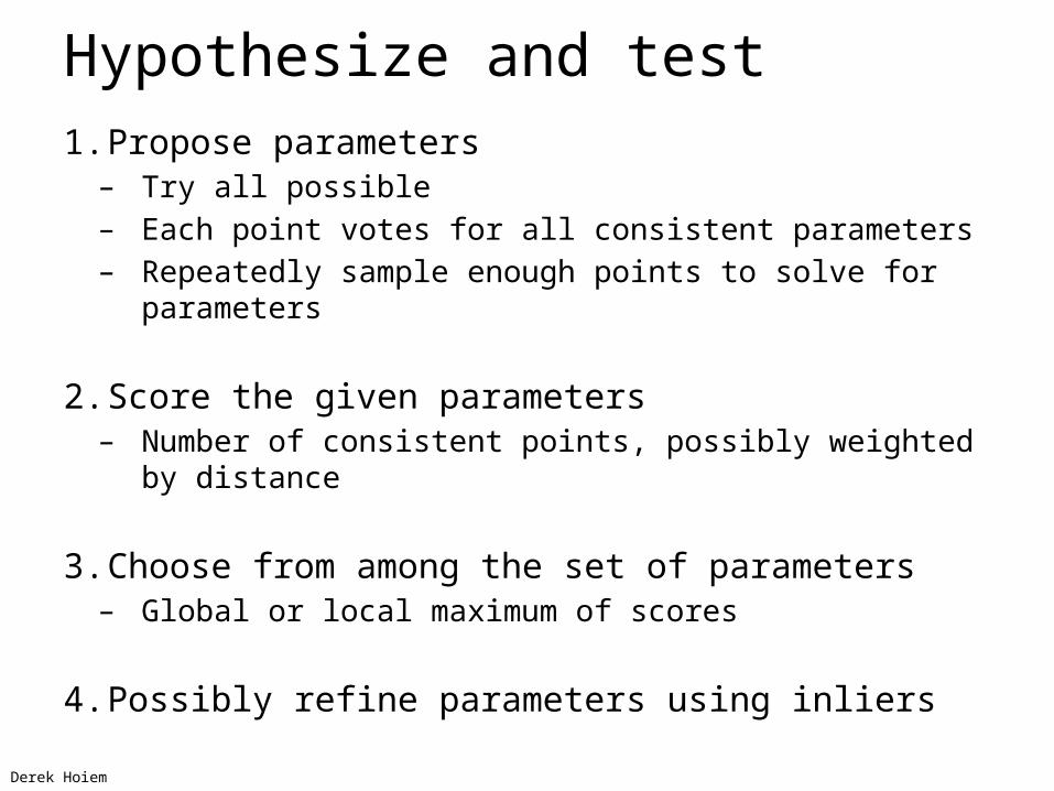
Hypothesize and test1. Propose parameters
– Try all possible– Each point votes for all consistent parameters– Repeatedly sample enough points to solve for parameters
2. Score the given parameters– Number of consistent points, possibly weighted by
distance
3. Choose from among the set of parameters– Global or local maximum of scores
4. Possibly refine parameters using inliersDerek Hoiem

Voting• It’s not feasible to check all combinations of features by
fitting a model to each possible subset.
• Voting is a general technique where we let the features vote for all models that are compatible with it.
– Cycle through features, cast votes for model parameters.
– Look for model parameters that receive a lot of votes.
• Noise & clutter features?
– They will cast votes too, but typically their votes should be inconsistent with the majority of “good” features.
Kristen Grauman
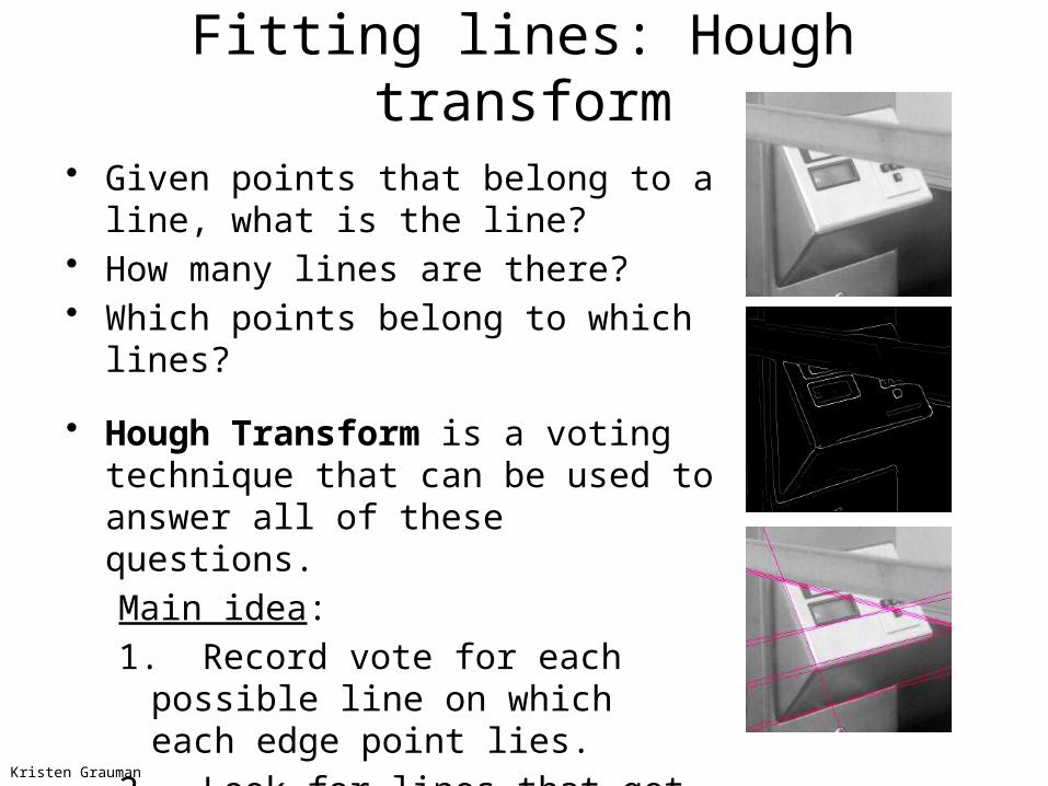
Fitting lines: Hough transform
• Given points that belong to a line, what is the line?
• How many lines are there?• Which points belong to which lines?
• Hough Transform is a voting technique that can be used to answer all of these questions.
Main idea:
1. Record vote for each possible line on which each edge point lies.
2. Look for lines that get many votes.
Kristen Grauman
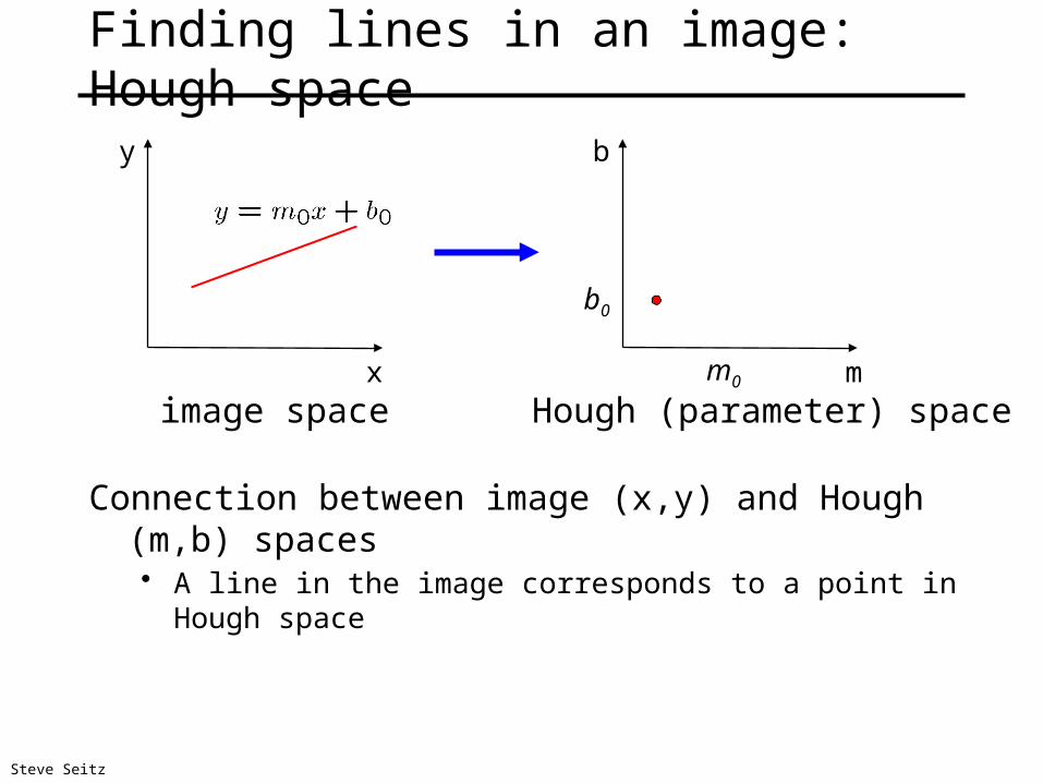
Finding lines in an image: Hough space
Connection between image (x,y) and Hough (m,b) spaces• A line in the image corresponds to a point in Hough space
x
y
m
b
m0
b0
image space Hough (parameter) space
Steve Seitz

Finding lines in an image: Hough space
Connection between image (x,y) and Hough (m,b) spaces• A line in the image corresponds to a point in Hough space• What does a point (x0, y0) in the image space map to?
• To go from image space to Hough space:– given a set of points (x,y), find all (m,b) such that y = mx + b
x
y
m
b
image space Hough (parameter) space
– Answer: the solutions of b = -x0m + y0
– This is a line in Hough space
x0
y0
Steve Seitz

Finding lines in an image: Hough space
What are the line parameters for the line that contains both (x0, y0) and (x1, y1)?• It is the intersection of the lines b = –x0m + y0 and
b = –x1m + y1
x
y
m
b
image space Hough (parameter) spacex0
y0
b = –x1m + y1
(x0, y0)
(x1, y1)
Steve Seitz

Finding lines in an image: Hough algorithm
How can we use this to find the most likely parameters (m,b) for the most prominent line in the image space?
• Let each edge point in image space vote for a set of possible parameters in Hough space
• Accumulate votes in discrete set of bins; parameters with the most votes indicate line in image space.
x
y
m
b
image space Hough (parameter) space
Steve Seitz

x
y
b
m
x
y m3 5 3 3 2 2
3 7 11 10 4 3
2 3 1 4 5 2
2 1 0 1 3 3
b
Hough transform
Silvio Savarese

• Problems with the (m,b) space:• Unbounded parameter domains• Vertical lines require infinite m
Parameter space representation
Svetlana Lazebnik

• Problems with the (m,b) space:• Unbounded parameter domains• Vertical lines require infinite m
• Alternative: polar representation
Parameter space representation
sincos yx
Each point (x,y) will add a sinusoid in the (,) parameter space
Svetlana Lazebnik

x
y
Hough transformP.V.C. Hough, Machine Analysis of Bubble Chamber Pictures, Proc. Int. Conf. High Energy Accelerators and Instrumentation, 1959
Hough space
siny cosx
Use a polar representation for the parameter space
Silvio Savarese

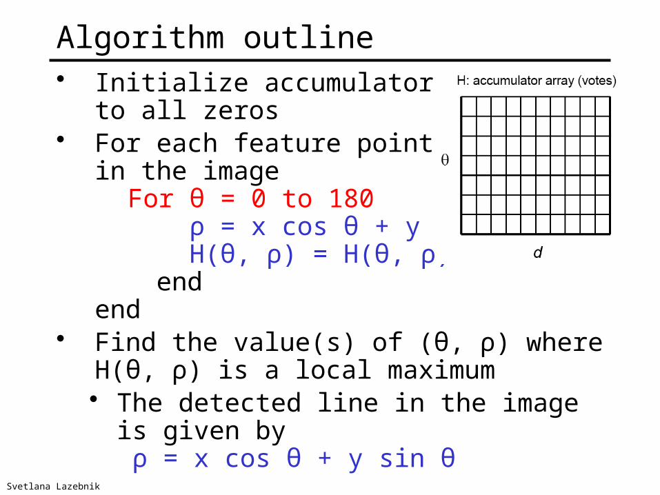
Algorithm outline• Initialize accumulator H
to all zeros• For each feature point (x,y)
in the imageFor θ = 0 to 180 ρ = x cos θ + y sin θ H(θ, ρ) = H(θ, ρ) + 1
endend
• Find the value(s) of (θ*, ρ*) where H(θ, ρ) is a local maximum• The detected line in the image is given by
ρ* = x cos θ* + y sin θ*
ρ
θ
Svetlana Lazebnik

Hough transform example
http://ostatic.com/files/images/ss_hough.jpgDerek Hoiem
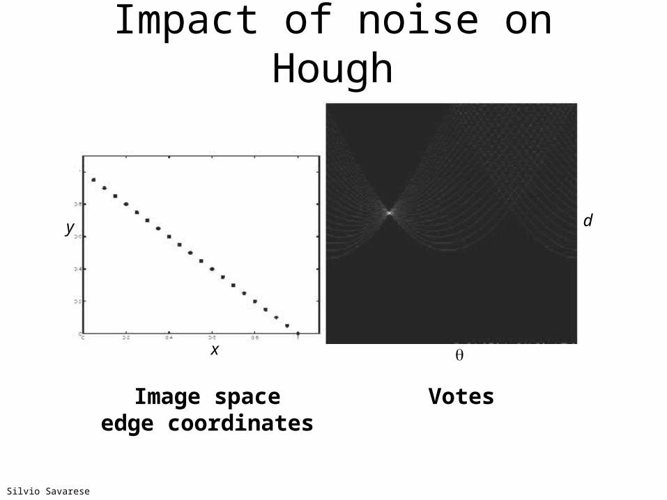
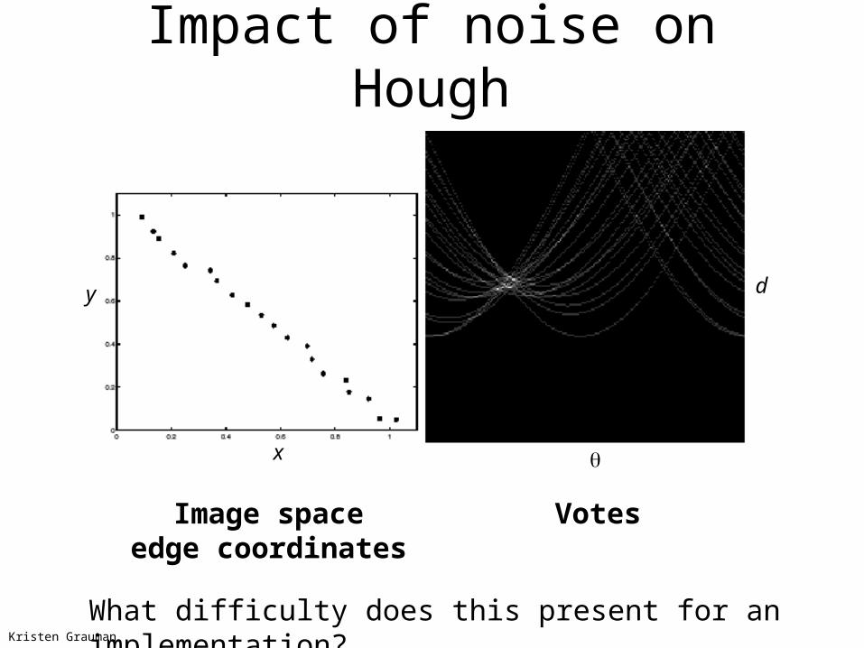
Impact of noise on Hough
Image spaceedge coordinates
Votes
x
d
Silvio Savarese
y
Impact of noise on Hough
Image spaceedge coordinates
Votes
x
y d
What difficulty does this present for an implementation?Kristen Grauman
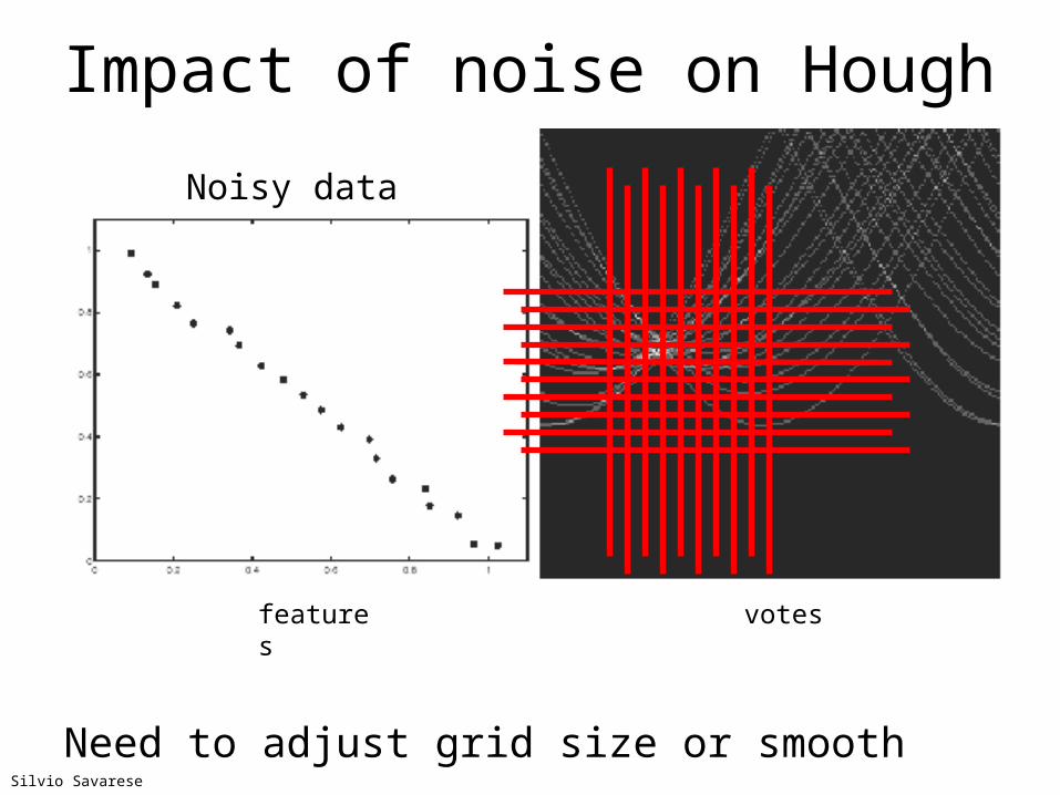
features votes
Need to adjust grid size or smooth
Noisy data
Silvio Savarese
Impact of noise on Hough
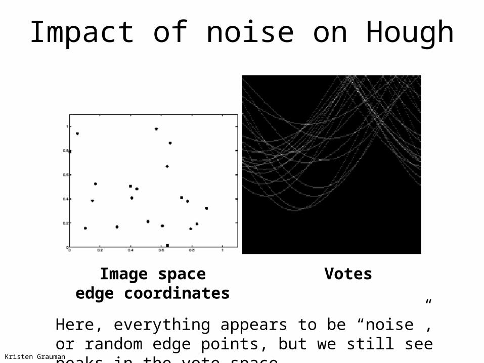
Image spaceedge coordinates
Votes
Impact of noise on Hough
Here, everything appears to be “noise”, or random edge points, but we still see peaks in the vote space.
Kristen Grauman
Algorithm outline• Initialize accumulator H
to all zeros• For each feature point (x,y)
in the imageFor θ = 0 to 180 ρ = x cos θ + y sin θ H(θ, ρ) = H(θ, ρ) + 1
endend
• Find the value(s) of (θ, ρ) where H(θ, ρ) is a local maximum• The detected line in the image is given by
ρ = x cos θ + y sin θ
ρ
θ
Svetlana Lazebnik

Incorporating image gradients• Recall: when we detect an
edge point, we also know its gradient direction
• But this means that the line is uniquely determined!
• Modified Hough transform:
For each edge point (x,y) θ = gradient orientation at (x,y)ρ = x cos θ + y sin θH(θ, ρ) = H(θ, ρ) + 1
end
Svetlana Lazebnik

• For a fixed radius r, unknown gradient direction
• Circle: center (a,b) and radius r222 )()( rbyax ii
Image space Hough space a
b
Kristen Grauman
Hough transform for circles

• For a fixed radius r, unknown gradient direction
• Circle: center (a,b) and radius r222 )()( rbyax ii
Image space Hough space
Intersection: most votes for center occur here.
Kristen Grauman
Hough transform for circles

• For an unknown radius r, unknown gradient direction
• Circle: center (a,b) and radius r222 )()( rbyax ii
Hough spaceImage space
b
a
r
?
Kristen Grauman
Hough transform for circles

• For an unknown radius r, unknown gradient direction
• Circle: center (a, b) and radius r222 )()( rbyax ii
Hough spaceImage space
b
a
r
Kristen Grauman
Hough transform for circles

Hough transform for circles
For every edge pixel (x,y) :
For all a:
For all b:
r =
H[a,b,r] += 1
end
end
end

• For an unknown radius r, known gradient direction
• Circle: center (a,b) and radius r222 )()( rbyax ii
Hough spaceImage space
θ
x
Kristen Grauman
Hough transform for circles

Hough transform for circles
• A circle with radius r and center (a, b) can be described as:
x = a + r cos(θ)
y = b + r sin(θ)
(a, b)
(x, y)

Hough transform for circles
For every edge pixel (x,y) :
For each possible radius value r:
For each possible gradient direction θ:
// or use estimated gradient at (x,y)
a = x – r cos(θ) // column
b = y – r sin(θ) // row
H[a,b,r] += 1
end
end
endModified from Kristen Grauman
θ
x
x = a + r cos(θ)y = b + r sin(θ)

Original Edges
Example: detecting circles with Hough
Votes: Penny
Note: a different Hough transform (with separate accumulators) was used for each circle radius (quarters vs. penny).
Kristen Grauman, images from Vivek Kwatra

Original Edges
Example: detecting circles with Hough
Votes: QuarterCombined detections
Kristen Grauman, images from Vivek Kwatra
Note: a different Hough transform (with separate accumulators) was used for each circle radius (quarters vs. penny).

Example: iris detection
• Hemerson Pistori and Eduardo Rocha Costa http://rsbweb.nih.gov/ij/plugins/hough-circles.html
Gradient+threshold Hough space (fixed radius)
Max detections
Kristen Grauman

Voting: practical tips
• Minimize irrelevant tokens first
• Choose a good grid / discretization
– Too coarse: large votes obtained when too many different lines correspond to a single bucket– Too fine: miss lines because points that are not exactly collinear cast votes for different buckets
• Vote for neighbors, also (smoothing in accumulator array)
• Use direction of edge to reduce parameters by 1
• To read back which points voted for “winning” peaks, keep tags on the votes
Too coarseToo fine ?
Kristen Grauman

Generalized Hough transform• We want to find a template defined by its
reference point (center) and several distinct types of landmark points in stable spatial configuration
c
Template
Svetlana Lazebnik

Model image Vote spaceNovel image
xxx
x
x
Now suppose those colors encode gradient directions…
• What if we want to detect arbitrary shapes?
Intuition:
Ref. point
Displacement vectors
Kristen Grauman
Generalized Hough transform

Define a model shape by its boundary points and a reference point.
[Dana H. Ballard, Generalizing the Hough Transform to Detect Arbitrary Shapes, 1980]
x a
p1
θ
p2
θ
At each boundary point, compute displacement vector: r = a – pi.
Store these vectors in a table indexed by gradient orientation θ.
Offline procedure:
Model shape
θ
θ
…
…
…
Kristen Grauman
Generalized Hough transform

p1
θ θ
For each edge point:• Use its gradient orientation θ
to index into stored table
• Use retrieved r vectors to vote for reference point
Detection procedure:
Assuming translation is the only transformation here, i.e., orientation and scale are fixed.
x
θ θ
Novel image
θ
θ
…
…
…
θ
xx
xx
Kristen Grauman
Generalized Hough transform

Generalized Hough transform• Template representation:
for each type of landmark point, store all possible displacement vectors towards the center
Model
Template
Svetlana Lazebnik

Generalized Hough transform• Detecting the template:
• For each feature in a new image, look up that feature type in the model and vote for the possible center locations associated with that type in the model
Model
Test image
Svetlana Lazebnik

Generalized Hough for object detection• Index displacements by “visual codeword”
B. Leibe, A. Leonardis, and B. Schiele, Combined Object Categorization and Segmentation with an Implicit Shape Model, ECCV Workshop on Statistical Learning in Computer Vision 2004
training image
“visual codeword” withdisplacement vectors
Svetlana Lazebnik

• Index displacements by “visual codeword”
test image
Generalized Hough for object detection
B. Leibe, A. Leonardis, and B. Schiele, Combined Object Categorization and Segmentation with an Implicit Shape Model, ECCV Workshop on Statistical Learning in Computer Vision 2004
Svetlana Lazebnik

Implicit shape models: Training
1. Build codebook of patches around extracted interest points using clustering (more on this later in the course)
Svetlana Lazebnik

Generalized Hough transform• Template representation:
for each type of landmark point, store all possible displacement vectors towards the center
Model
Template
Svetlana Lazebnik

Implicit shape models: Training
1. Build codebook of patches around extracted interest points using clustering
2. Map the patch around each interest point to closest codebook entry
Svetlana Lazebnik

Implicit shape models: Training
1. Build codebook of patches around extracted interest points using clustering
2. Map the patch around each interest point to closest codebook entry
3. For each codebook entry, store all positions it was found, relative to object center
Svetlana Lazebnik

Hough transform: pros and cons
Pros• All points are processed independently, so can cope with
occlusion, gaps• Some robustness to noise: noise points unlikely to
contribute consistently to any single bin• Can detect multiple instances of a model in a single pass
Cons• Complexity of search time increases exponentially with
the number of model parameters • Non-target shapes can produce spurious peaks in
parameter space• Quantization: can be tricky to pick a good grid size
Kristen Grauman

Today
• Fitting models (lines) to points, i.e. find the parameters of a model that best fits the data– Least squares– Hough transform– RANSAC
• Matching = finding correspondences between points, i.e. find the parameters of the transformation that best aligns points
• Homework 2 is due 10/08

Outliers• Outliers can hurt the quality of our parameter
estimates, e.g., – an erroneous pair of matching points from two images– an edge point that is noise, or doesn’t belong to the
line we are fitting.
Kristen Grauman

Outliers affect least squares fit
Kristen Grauman

Outliers affect least squares fit
Kristen Grauman

RANSAC
• RANdom Sample Consensus
• Approach: we want to avoid the impact of outliers, so let’s look for “inliers”, and use those only.
• Intuition: if an outlier is chosen to compute the current fit, then the resulting line won’t have much support from rest of the points.
Kristen Grauman

RANSAC: General form
• RANSAC loop:
1. Randomly select a seed group of s points on which to base model estimate
2. Fit model to these s points
3. Find inliers to this model (i.e., points whose distance from the line is less than t)
4. If there are d or more inliers, re-compute estimate of model on all of the inliers
5. Repeat N times
• Keep the model with the largest number of inliers
Modified from Kristen Grauman and Svetlana Lazebnik

RANSAC for line fitting example
Source: R. Raguram

RANSAC for line fitting example
Least-squares fit
Source: R. Raguram

RANSAC for line fitting example
1. Randomly select minimal subset of points
Source: R. Raguram

RANSAC for line fitting example
1. Randomly select minimal subset of points
2. Hypothesize a model
Source: R. Raguram

RANSAC for line fitting example
1. Randomly select minimal subset of points
2. Hypothesize a model
3. Compute error function
Source: R. Raguram

RANSAC for line fitting example
1. Randomly select minimal subset of points
2. Hypothesize a model
3. Compute error function
4. Select points consistent with model
Source: R. Raguram

RANSAC for line fitting example
1. Randomly select minimal subset of points
2. Hypothesize a model
3. Compute error function
4. Select points consistent with model
5. Repeat hypothesize-and-verify loop
Source: R. Raguram

1. Randomly select minimal subset of points
2. Hypothesize a model
3. Compute error function
4. Select points consistent with model
5. Repeat hypothesize-and-verify loop
RANSAC for line fitting example
Source: R. Raguram

1. Randomly select minimal subset of points
2. Hypothesize a model
3. Compute error function
4. Select points consistent with model
5. Repeat hypothesize-and-verify loop
RANSAC for line fitting example
Uncontaminated sample
Source: R. Raguram

RANSAC for line fitting example
1. Randomly select minimal subset of points
2. Hypothesize a model
3. Compute error function
4. Select points consistent with model
5. Repeat hypothesize-and-verify loop
Source: R. Raguram

RANSAC
Algorithm:
1. Sample (randomly) the number of points required to fit the model2. Solve for model parameters using samples 3. Score by the fraction of inliers within a preset threshold of the model
Repeat 1-3 until the best model is found with high confidence
Fischler & Bolles in ‘81.
(RANdom SAmple Consensus) :
Silvio Savarese
RANSAC
Algorithm:
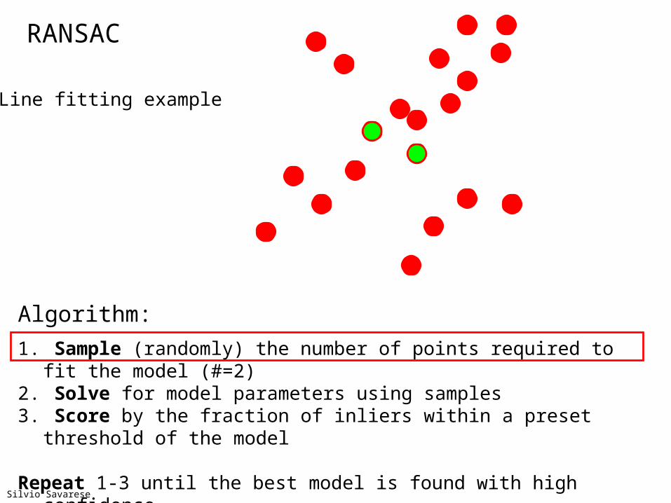
1. Sample (randomly) the number of points required to fit the model (#=2)2. Solve for model parameters using samples 3. Score by the fraction of inliers within a preset threshold of the model
Repeat 1-3 until the best model is found with high confidence
Line fitting example
Silvio Savarese
RANSAC
Algorithm:
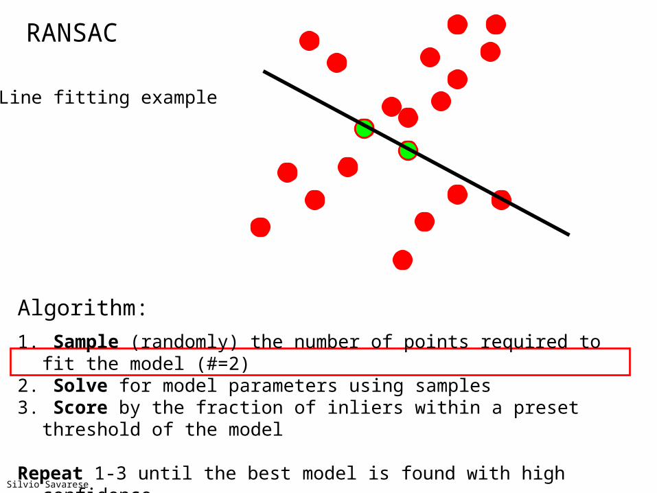
1. Sample (randomly) the number of points required to fit the model (#=2)2. Solve for model parameters using samples 3. Score by the fraction of inliers within a preset threshold of the model
Repeat 1-3 until the best model is found with high confidence
Line fitting example
Silvio Savarese

RANSAC
6IN
Algorithm:
1. Sample (randomly) the number of points required to fit the model (#=2)2. Solve for model parameters using samples 3. Score by the fraction of inliers within a preset threshold of the model
Repeat 1-3 until the best model is found with high confidence
Line fitting example
Silvio Savarese
RANSAC
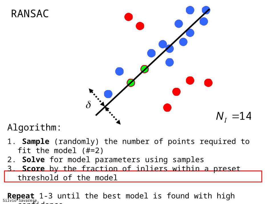
14INAlgorithm:
1. Sample (randomly) the number of points required to fit the model (#=2)2. Solve for model parameters using samples 3. Score by the fraction of inliers within a preset threshold of the model
Repeat 1-3 until the best model is found with high confidence
Silvio Savarese

How to choose parameters?• Number of samples N
– Choose N so that, with probability p, at least one random sample is free from outliers (e.g. p=0.99) (outlier ratio: e )
• Number of sampled points s– Minimum number needed to fit the model
• Distance threshold – Choose so that a good point with noise is likely (e.g., prob=0.95) within threshold
proportion of outliers es 5% 10% 20% 25% 30% 40% 50%2 2 3 5 6 7 11 173 3 4 7 9 11 19 354 3 5 9 13 17 34 725 4 6 12 17 26 57 1466 4 7 16 24 37 97 2937 4 8 20 33 54 163 5888 5 9 26 44 78 272 117
7Marc Pollefeys and Derek Hoiem
se11log/p1logN
Explanation in Szeliski 6.1.4

RANSAC pros and cons• Pros
• Simple and general• Applicable to many different problems• Often works well in practice
• Cons• Lots of parameters to tune• Doesn’t work well for low inlier ratios (too many iterations,
or can fail completely)• Can’t always get a good initialization
of the model based on the minimum number of samples
• Common applications• Image stitching• Relating two views
Svetlana Lazebnik