Embed Size (px)
Citation preview
CS 2770: Computer Vision
Neural Networks
Prof. Adriana KovashkaUniversity of Pittsburgh
January 19, 2017
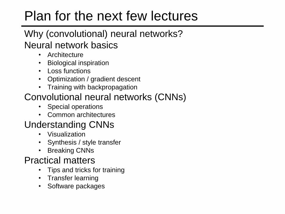
Plan for the next few lectures
Why (convolutional) neural networks?
Neural network basics• Architecture
• Biological inspiration
• Loss functions
• Optimization / gradient descent
• Training with backpropagation
Convolutional neural networks (CNNs)• Special operations
• Common architectures
Understanding CNNs• Visualization
• Synthesis / style transfer
• Breaking CNNs
Practical matters• Tips and tricks for training
• Transfer learning
• Software packages
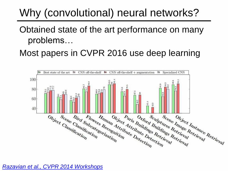
Why (convolutional) neural networks?
Obtained state of the art performance on many
problems…
Most papers in CVPR 2016 use deep learning
Razavian et al., CVPR 2014 Workshops
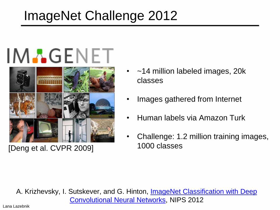
ImageNet Challenge 2012
Validation classification
Validation classification
Validation classification
[Deng et al. CVPR 2009]
• ~14 million labeled images, 20k
classes
• Images gathered from Internet
• Human labels via Amazon Turk
• Challenge: 1.2 million training images,
1000 classes
A. Krizhevsky, I. Sutskever, and G. Hinton, ImageNet Classification with Deep
Convolutional Neural Networks, NIPS 2012Lana Lazebnik
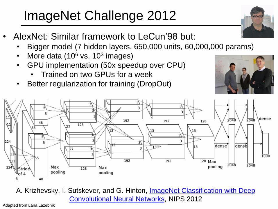
ImageNet Challenge 2012
• AlexNet: Similar framework to LeCun’98 but:• Bigger model (7 hidden layers, 650,000 units, 60,000,000 params)
• More data (106 vs. 103 images)
• GPU implementation (50x speedup over CPU)
• Trained on two GPUs for a week
• Better regularization for training (DropOut)
A. Krizhevsky, I. Sutskever, and G. Hinton, ImageNet Classification with Deep
Convolutional Neural Networks, NIPS 2012Adapted from Lana Lazebnik
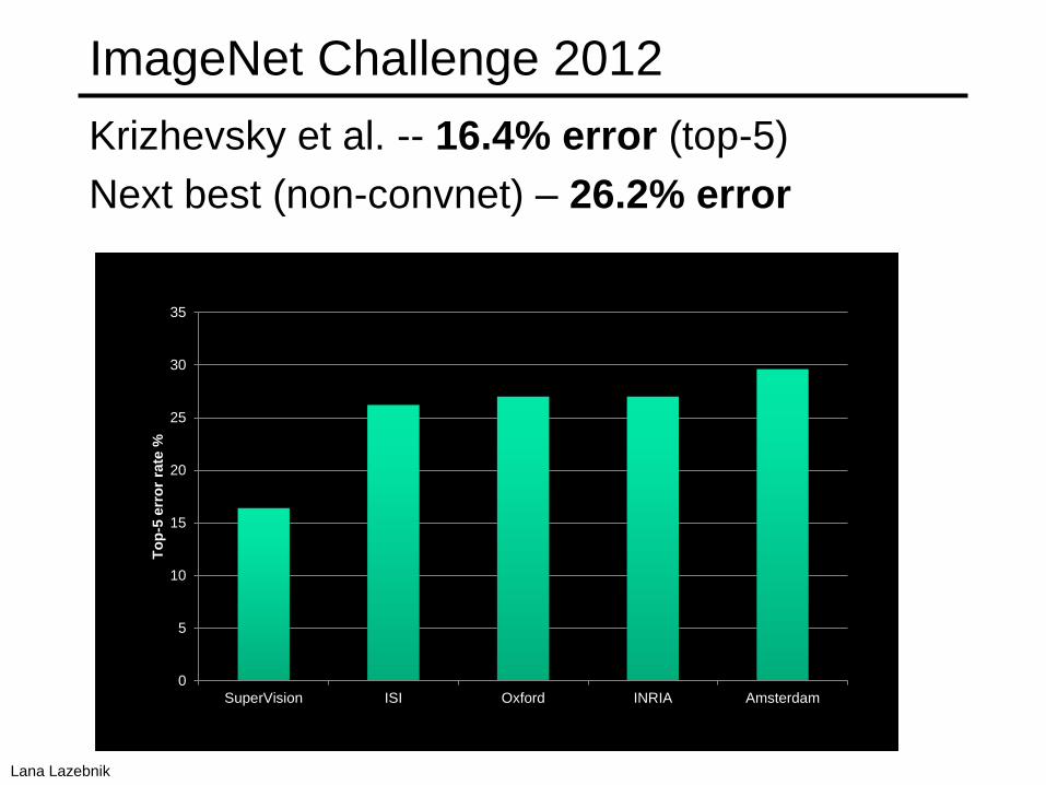
ImageNet Challenge 2012
Krizhevsky et al. -- 16.4% error (top-5)
Next best (non-convnet) – 26.2% error
0
5
10
15
20
25
30
35
SuperVision ISI Oxford INRIA Amsterdam
To
p-5
err
or
rate
%
Lana Lazebnik
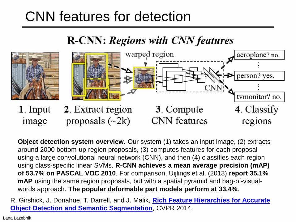
CNN features for detection
Object detection system overview. Our system (1) takes an input image, (2) extracts
around 2000 bottom-up region proposals, (3) computes features for each proposal
using a large convolutional neural network (CNN), and then (4) classifies each region
using class-specific linear SVMs. R-CNN achieves a mean average precision (mAP)
of 53.7% on PASCAL VOC 2010. For comparison, Uijlings et al. (2013) report 35.1%
mAP using the same region proposals, but with a spatial pyramid and bag-of-visual-
words approach. The popular deformable part models perform at 33.4%.
R. Girshick, J. Donahue, T. Darrell, and J. Malik, Rich Feature Hierarchies for Accurate
Object Detection and Semantic Segmentation, CVPR 2014.
Lana Lazebnik
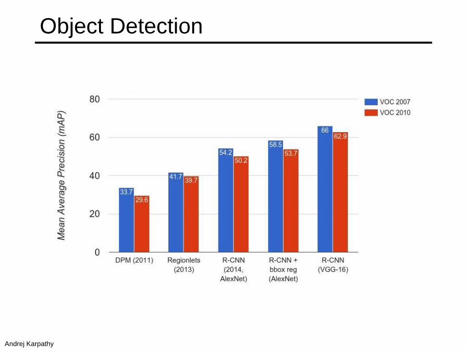
Object Detection
Andrej Karpathy
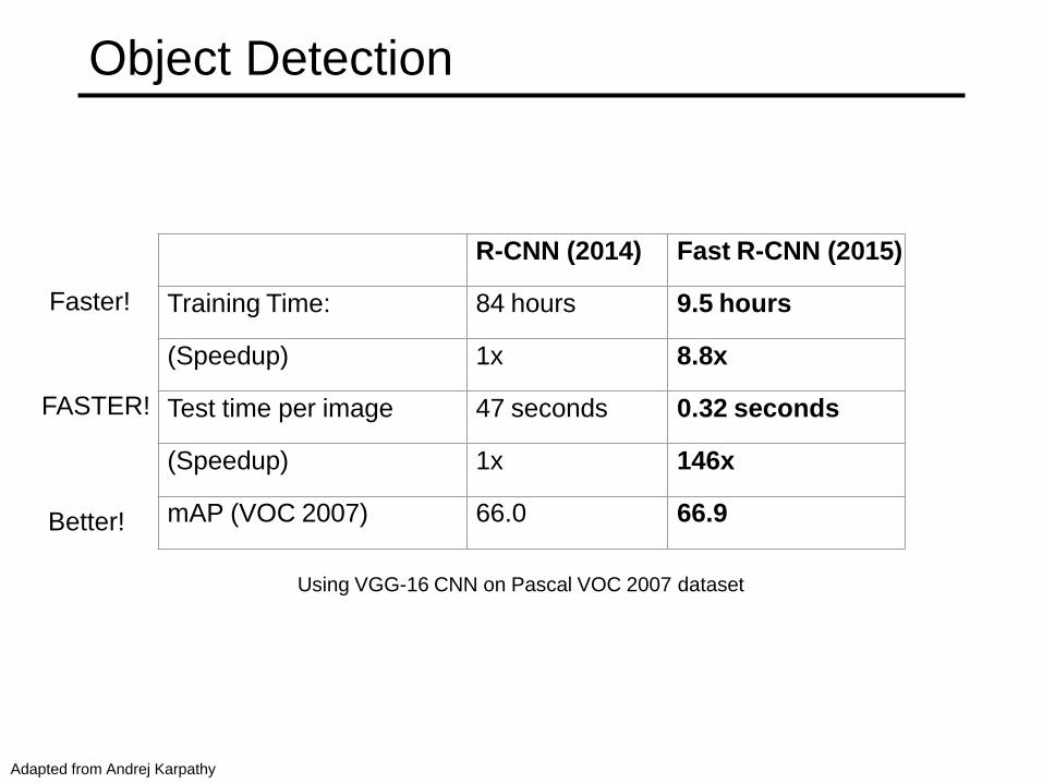
Object Detection
Using VGG-16 CNN on Pascal VOC 2007 dataset
R-CNN (2014) Fast R-CNN (2015)
Training Time: 84 hours 9.5 hours
(Speedup) 1x 8.8x
Test time per image 47 seconds 0.32 seconds
(Speedup) 1x 146x
mAP (VOC 2007) 66.0 66.9
Faster!
FASTER!
Better!
Adapted from Andrej Karpathy
Beyond classification
Detection
Segmentation
Regression
Pose estimation
Synthesis
and many more…
Adapted from Jia-bin Huang
What are CNNs?
• Convolutional neural networks are a type of
neural network
• The neural network includes layers that
perform special operations
• Used in vision, but to a lesser extent also in
NLP, biomedical, etc.
• Often they are deep
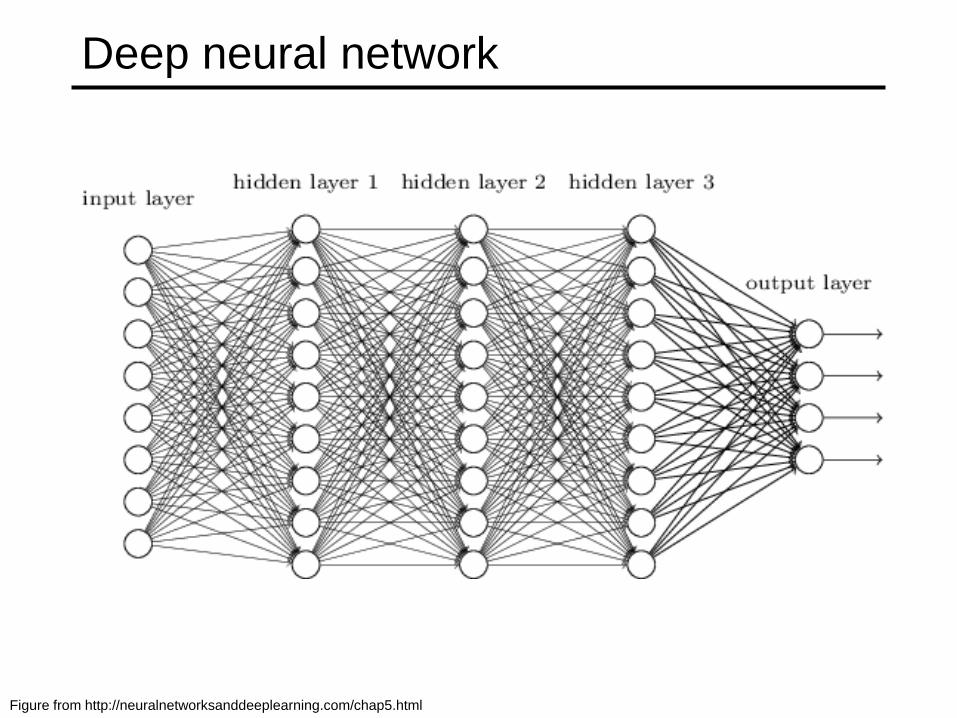
Deep neural network
Figure from http://neuralnetworksanddeeplearning.com/chap5.html
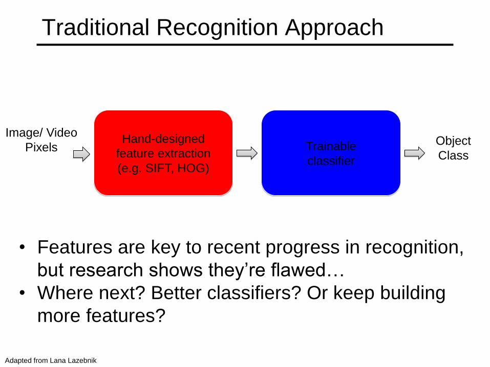
Traditional Recognition Approach
Hand-designed
feature extraction
(e.g. SIFT, HOG)
Trainable
classifier
Image/ Video
Pixels
• Features are key to recent progress in recognition,
but research shows they’re flawed…
• Where next? Better classifiers? Or keep building
more features?
Object
Class
Adapted from Lana Lazebnik
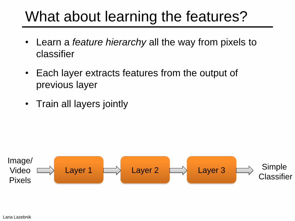
What about learning the features?
• Learn a feature hierarchy all the way from pixels to
classifier
• Each layer extracts features from the output of
previous layer
• Train all layers jointly
Layer 1 Layer 2 Layer 3 Simple
Classifier
Image/
Video
Pixels
Lana Lazebnik
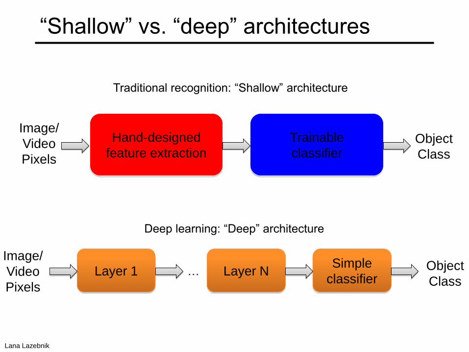
“Shallow” vs. “deep” architectures
Hand-designed
feature extraction
Trainable
classifier
Image/
Video
Pixels
Object
Class
Layer 1 Layer NSimple
classifierObject
Class
Image/
Video
Pixels
Traditional recognition: “Shallow” architecture
Deep learning: “Deep” architecture
…
Lana Lazebnik
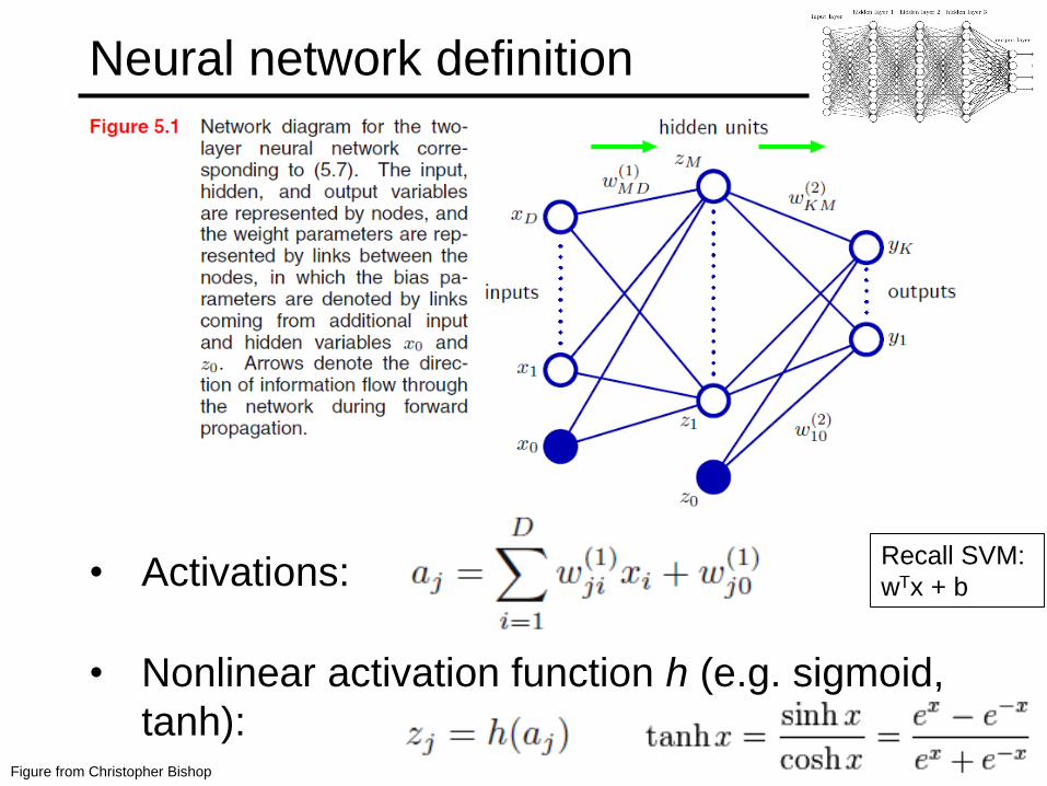
Neural network definition
• Activations:
• Nonlinear activation function h (e.g. sigmoid,
tanh):Figure from Christopher Bishop
Recall SVM:
wTx + b
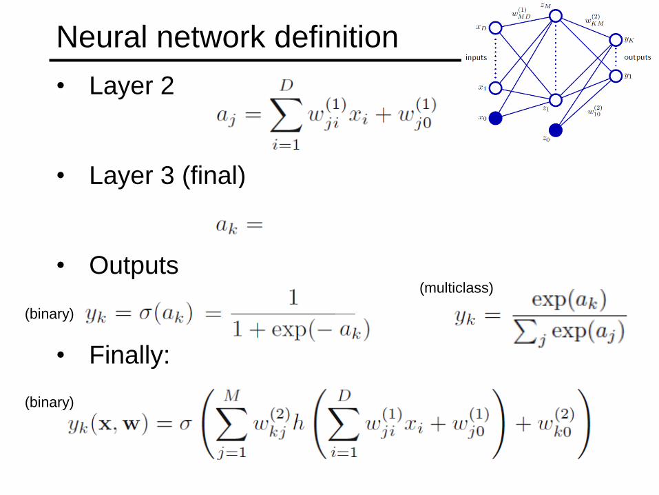
• Layer 2
• Layer 3 (final)
• Outputs
• Finally:
Neural network definition
(binary)
(multiclass)
(binary)
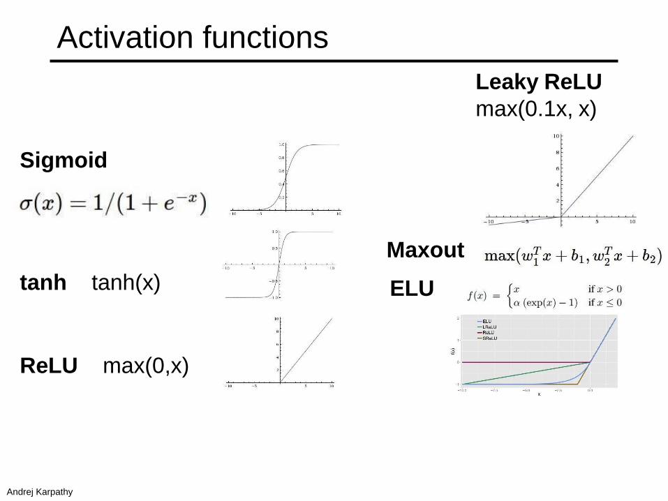
Sigmoid
tanh tanh(x)
ReLU max(0,x)
Leaky ReLU
max(0.1x, x)
Maxout
ELU
Activation functions
Andrej Karpathy
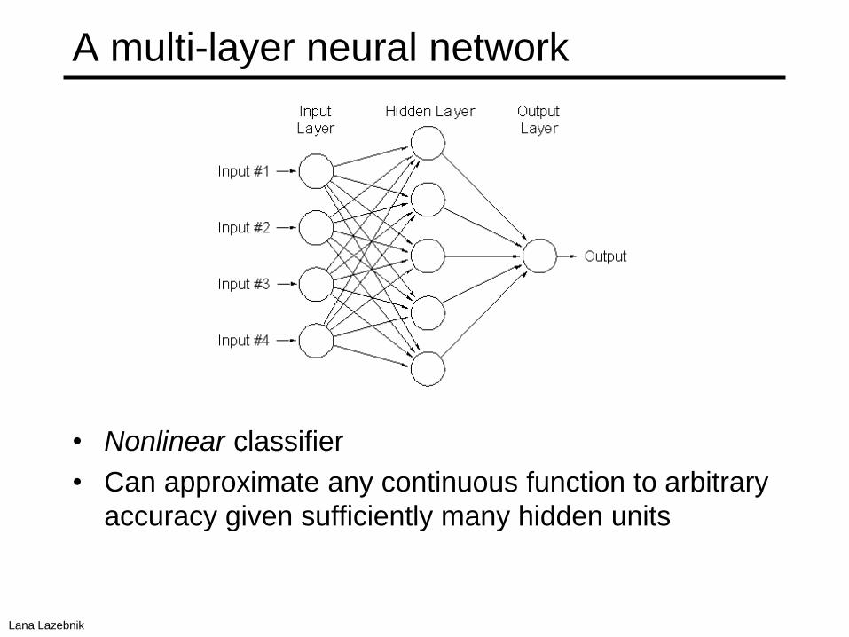
A multi-layer neural network
• Nonlinear classifier
• Can approximate any continuous function to arbitrary
accuracy given sufficiently many hidden units
Lana Lazebnik
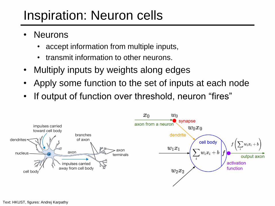
Inspiration: Neuron cells
• Neurons
• accept information from multiple inputs,
• transmit information to other neurons.
• Multiply inputs by weights along edges
• Apply some function to the set of inputs at each node
• If output of function over threshold, neuron “fires”
Text: HKUST, figures: Andrej Karpathy
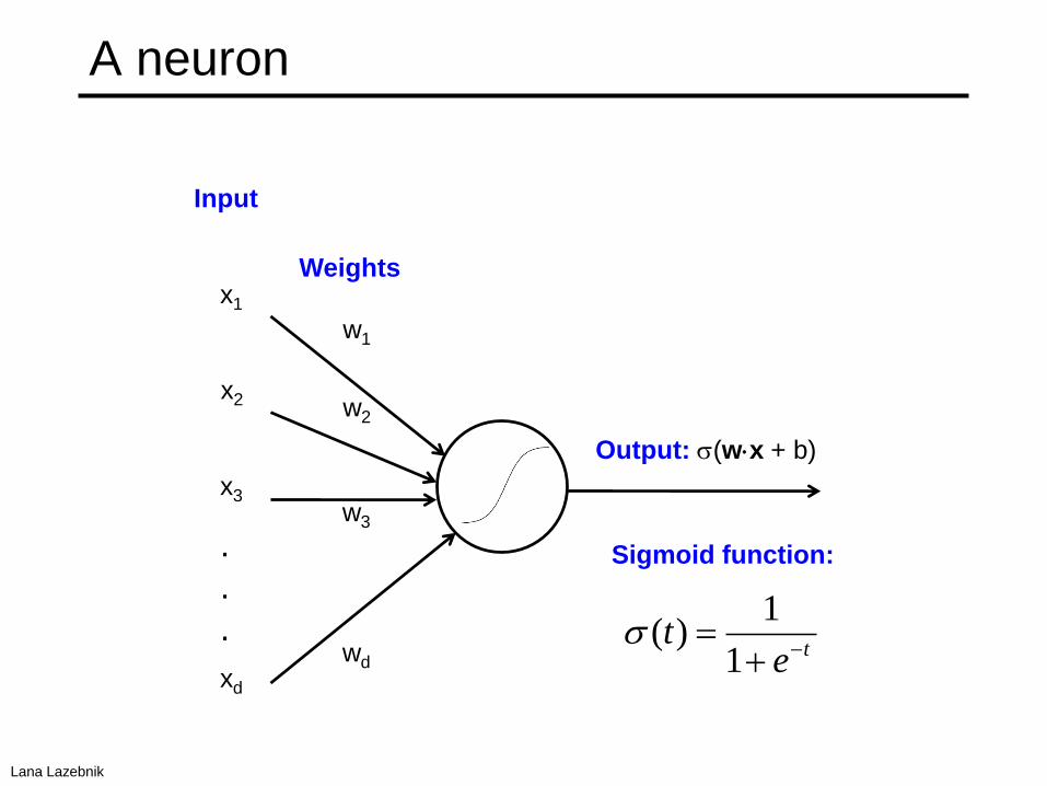
A neuron
x1
x2
xd
w1
w2
w3
x3
wd
Sigmoid function:
Input
Weights
.
.
.te
t
1
1)(
Output: (wx + b)
Lana Lazebnik
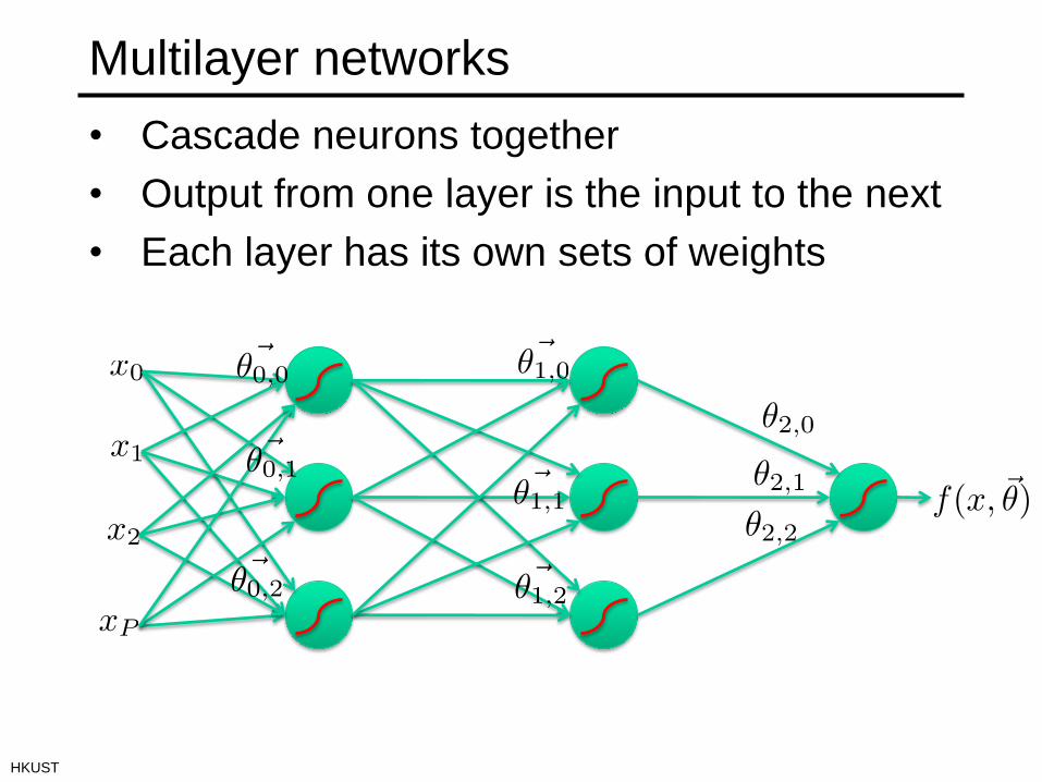
Multilayer networks
• Cascade neurons together
• Output from one layer is the input to the next
• Each layer has its own sets of weights
HKUST
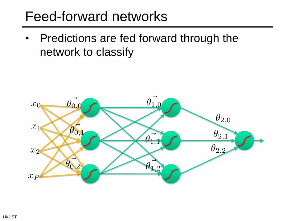
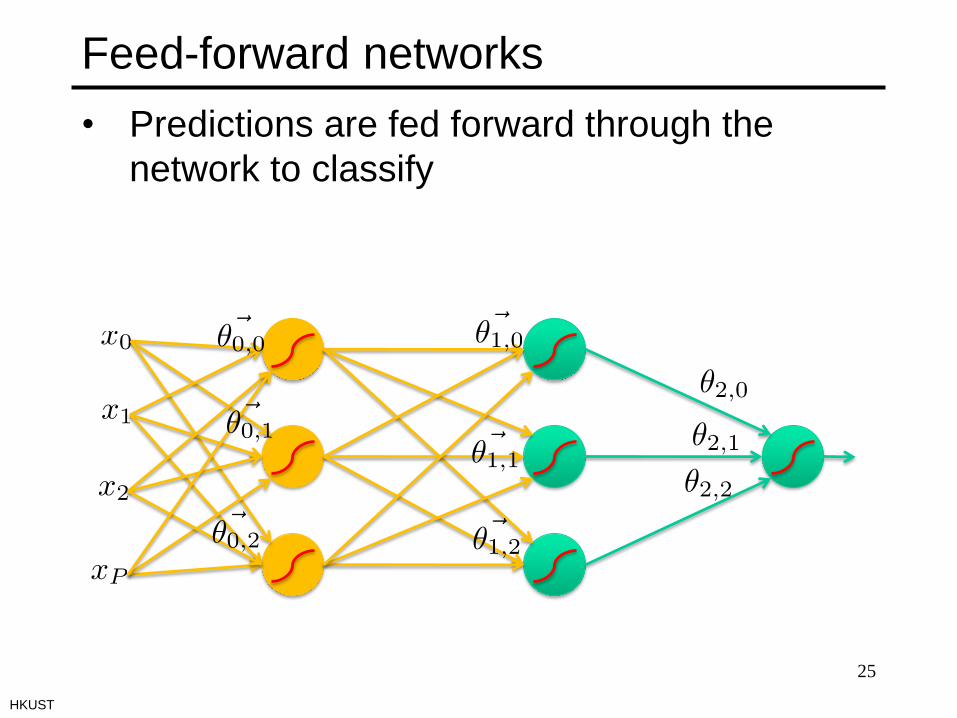
Feed-forward networks
• Predictions are fed forward through the
network to classify
HKUST
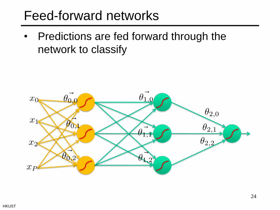
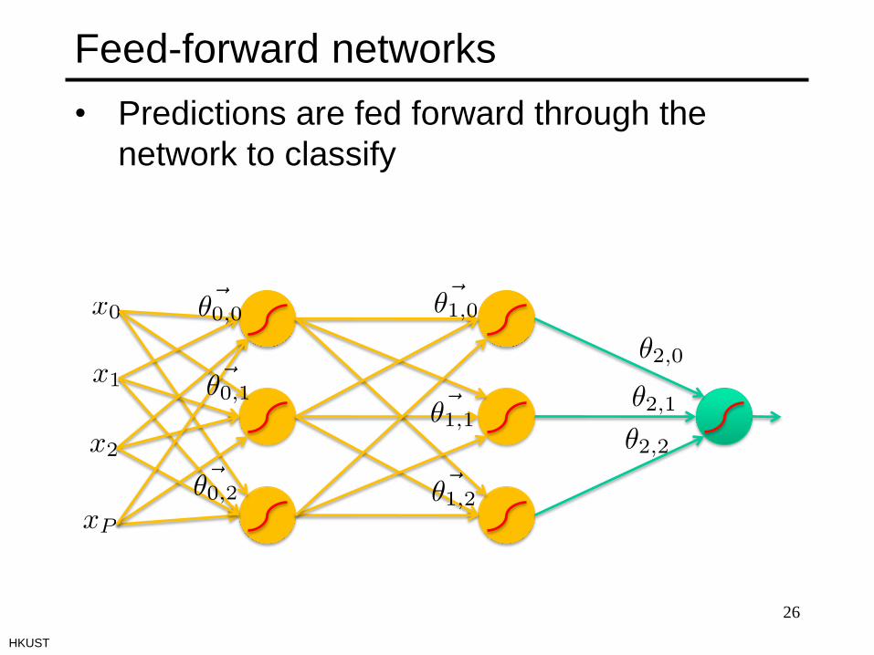
Feed-forward networks
24
• Predictions are fed forward through the
network to classify
HKUST
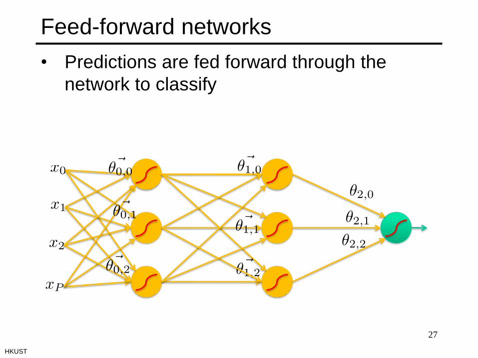
Feed-forward networks
25
• Predictions are fed forward through the
network to classify
HKUST
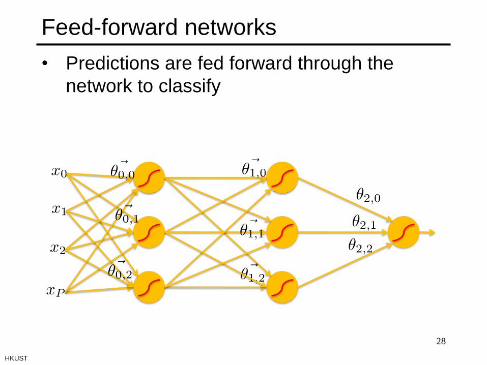
Feed-forward networks
26
• Predictions are fed forward through the
network to classify
HKUST
Feed-forward networks
27
• Predictions are fed forward through the
network to classify
HKUST
Feed-forward networks
28
• Predictions are fed forward through the
network to classify
HKUST
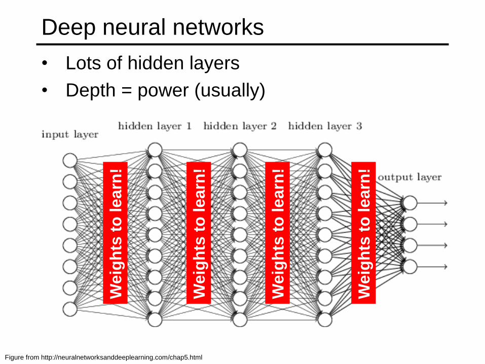
Deep neural networks
• Lots of hidden layers
• Depth = power (usually)
Figure from http://neuralnetworksanddeeplearning.com/chap5.html
We
igh
ts t
o lea
rn!
We
igh
ts t
o le
arn
!
We
igh
ts t
o lea
rn!
We
igh
ts t
o lea
rn!
How do we train them?
• The goal is to iteratively find such a set of
weights that allow the activations/outputs to
match the desired output
• We want to minimize a loss function
• The loss function is a function of the weights
in the network
• For now let’s simplify and assume there’s a
single layer of weights in the network
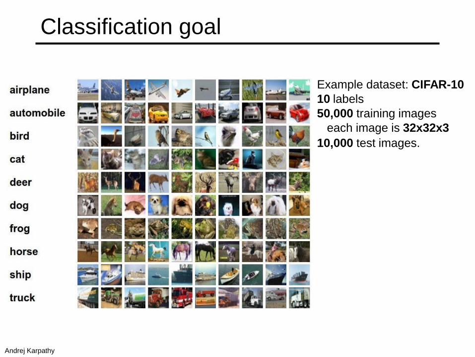
Classification goal
Example dataset: CIFAR-10
10 labels
50,000 training images
each image is 32x32x3
10,000 test images.
Andrej Karpathy
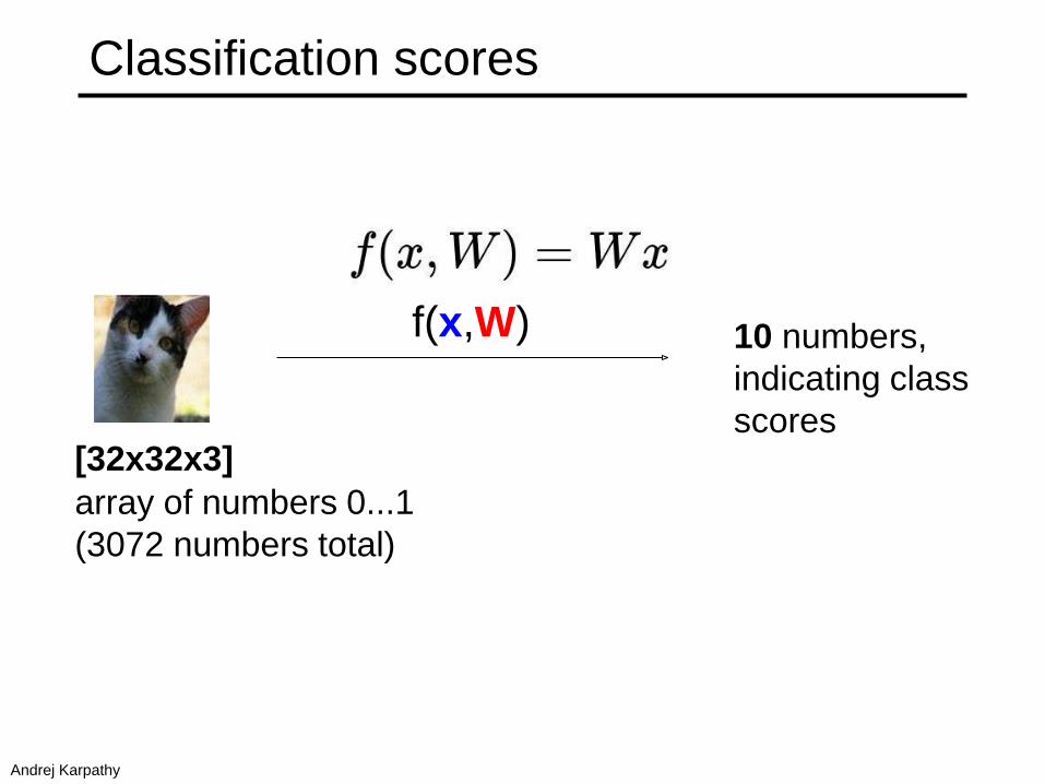
Classification scores
[32x32x3]
array of numbers 0...1
(3072 numbers total)
f(x,W)
image parameters
10 numbers,
indicating class
scores
Andrej Karpathy
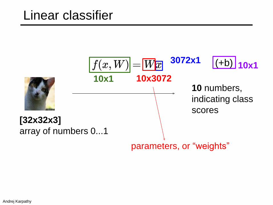
Linear classifier
[32x32x3]
array of numbers 0...1
10 numbers,
indicating class
scores
3072x1
10x1 10x3072
parameters, or “weights”
(+b) 10x1
Andrej Karpathy
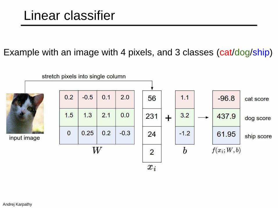
Linear classifier
Example with an image with 4 pixels, and 3 classes (cat/dog/ship)
Andrej Karpathy
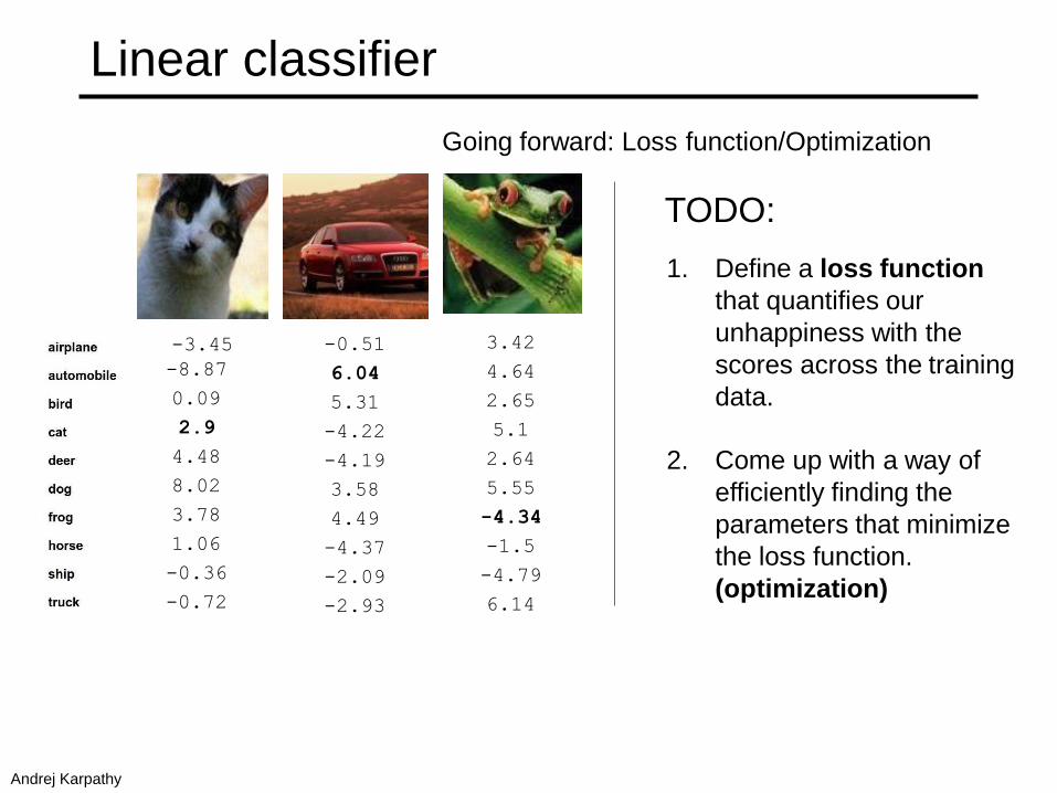
Linear classifier
Going forward: Loss function/Optimization
-3.45
-8.87
0.09
2.9
4.48
8.02
3.78
1.06
-0.36
-0.72
-0.51
6.04
5.31
-4.22
-4.19
3.58
4.49
-4.37
-2.09
-2.93
3.42
4.64
2.65
5.1
2.64
5.55
-4.34
-1.5
-4.79
6.14
1. Define a loss function
that quantifies our
unhappiness with the
scores across the training
data.
2. Come up with a way of
efficiently finding the
parameters that minimize
the loss function.
(optimization)
TODO:
Andrej Karpathy
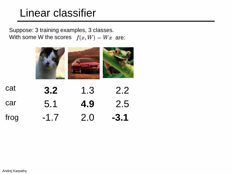
Linear classifier
Suppose: 3 training examples, 3 classes.
With some W the scores are:
cat
car
frog
3.2
5.1
-1.7
1.3
4.9
2.0
2.2
2.5
-3.1
Andrej Karpathy
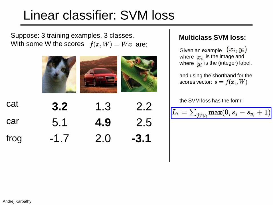
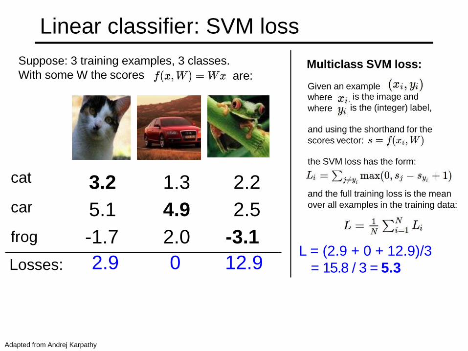
Linear classifier: SVM loss
Suppose: 3 training examples, 3 classes.
With some W the scores are:
cat
car
frog
3.2
5.1
-1.7
1.3
4.9
2.0
2.2
2.5
-3.1
Multiclass SVM loss:
Given an example
where
where
is the image and
is the (integer) label,
and using the shorthand for the
scores vector:
the SVM loss has the form:
Andrej Karpathy
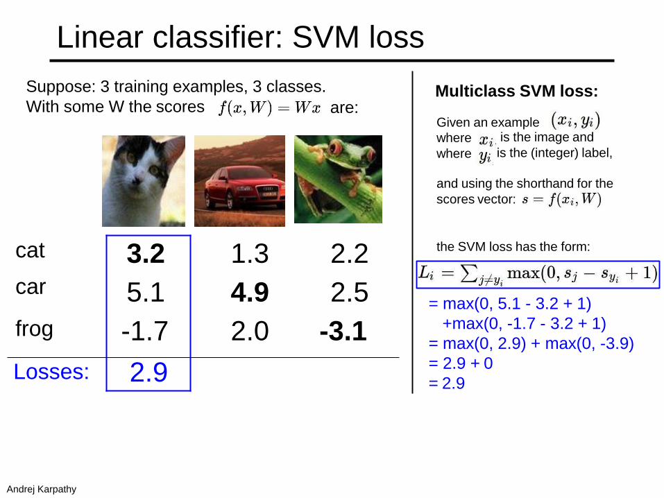
Linear classifier: SVM loss
Suppose: 3 training examples, 3 classes.
With some W the scores are:Multiclass SVM loss:
Given an example
where
where
is the image and
is the (integer) label,
and using the shorthand for the
scores vector:
the SVM loss has the form:
= max(0, 5.1 - 3.2 + 1)
+max(0, -1.7 - 3.2 + 1)
= max(0, 2.9) + max(0, -3.9)
= 2.9 + 0
= 2.9
cat
car
frog
3.2
5.1
-1.7
1.3 2.2
4.9 2.5
2.0 -3.1
Losses: 2.9
Andrej Karpathy
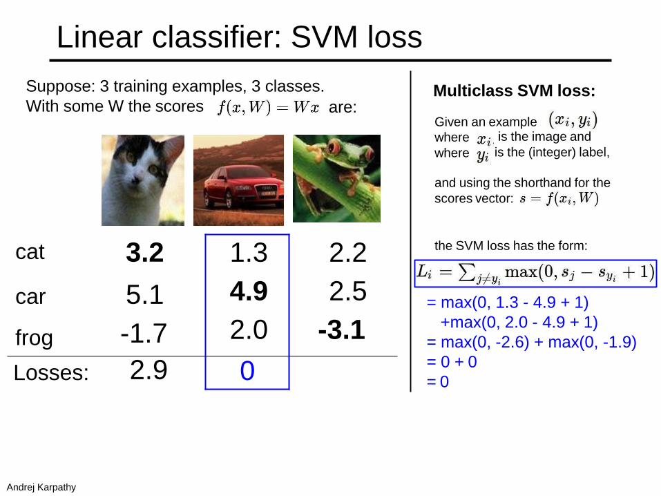
Linear classifier: SVM loss
Suppose: 3 training examples, 3 classes.
With some W the scores are:Multiclass SVM loss:
Given an example
where
where
is the image and
is the (integer) label,
and using the shorthand for the
scores vector:
the SVM loss has the form:
= max(0, 1.3 - 4.9 + 1)
+max(0, 2.0 - 4.9 + 1)
= max(0, -2.6) + max(0, -1.9)
= 0 + 0
= 0
cat 3.2
car 5.1
frog -1.7
1.3
4.9
2.0
2.2
2.5
-3.1
Losses: 2.9 0
Andrej Karpathy
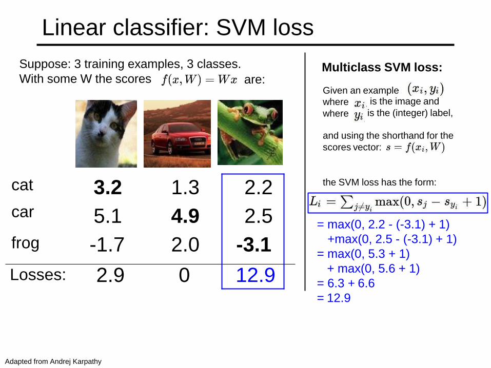
Linear classifier: SVM loss
Suppose: 3 training examples, 3 classes.
With some W the scores are:Multiclass SVM loss:
Given an example
where
where
is the image and
is the (integer) label,
and using the shorthand for the
scores vector:
the SVM loss has the form:
= max(0, 2.2 - (-3.1) + 1)
+max(0, 2.5 - (-3.1) + 1)
= max(0, 5.3 + 1)
+ max(0, 5.6 + 1)
= 6.3 + 6.6
= 12.9
cat
car
frog
3.2
5.1
-1.7
1.3
4.9
2.0
2.2
2.5
-3.1
Losses: 2.9 0 12.9
Adapted from Andrej Karpathy
Linear classifier: SVM loss
cat
car
frog
3.2
5.1
-1.7
1.3
4.9
2.0
2.2
2.5
-3.1
Suppose: 3 training examples, 3 classes.
With some W the scores are:Multiclass SVM loss:
Given an example
where
where
is the image and
is the (integer) label,
and using the shorthand for the
scores vector:
the SVM loss has the form:
and the full training loss is the mean
over all examples in the training data:
L = (2.9 + 0 + 12.9)/32.9 0 12.9Losses: = 15.8 / 3 = 5.3
Lecture 3 - 12
Adapted from Andrej Karpathy

Linear classifier: SVM loss
Andrej Karpathy
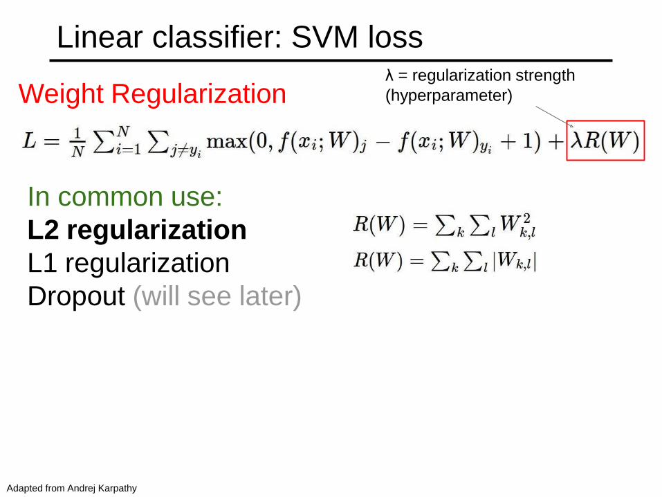
Linear classifier: SVM loss
Weight Regularizationλ = regularization strength
(hyperparameter)
In common use:
L2 regularization
L1 regularization
Dropout (will see later)
Adapted from Andrej Karpathy
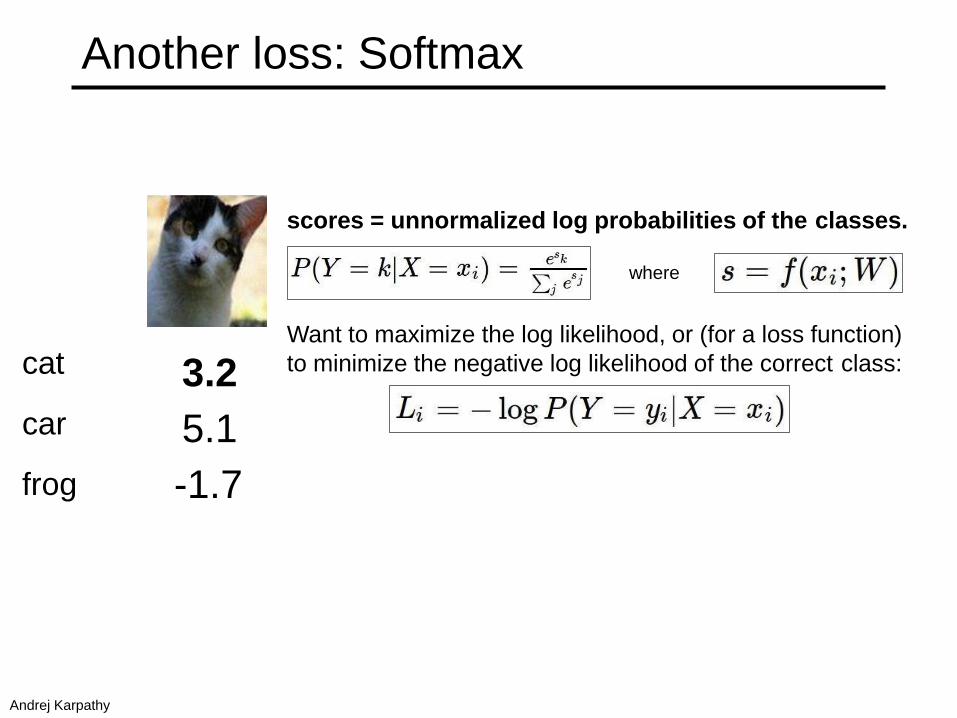
Want to maximize the log likelihood, or (for a loss function)
to minimize the negative log likelihood of the correct class:cat
car
frog
3.2
5.1
-1.7
scores = unnormalized log probabilities of the classes.
where
Another loss: Softmax
Andrej Karpathy
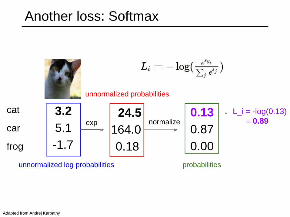
cat
car
frog
unnormalized log probabilities
24.5
164.0
0.18
3.2
5.1
-1.7
exp normalize
unnormalized probabilities
0.13
0.87
0.00
probabilities
L_i = -log(0.13)
= 0.89
Another loss: Softmax
Adapted from Andrej Karpathy
How to minimize the loss function?
Andrej Karpathy
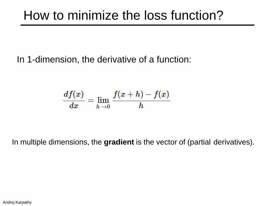
How to minimize the loss function?
In 1-dimension, the derivative of a function:
In multiple dimensions, the gradient is the vector of (partial derivatives).
Andrej Karpathy
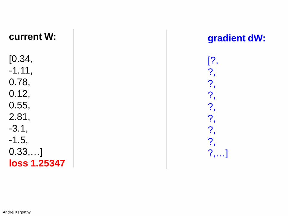
current W:
[0.34,
-1.11,
0.78,
0.12,
0.55,
2.81,
-3.1,
-1.5,
0.33,…]
loss 1.25347
gradient dW:
[?,
?,
?,
?,
?,
?,
?,
?,
?,…]
Andrej Karpathy
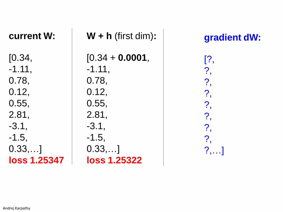
current W:
[0.34,
-1.11,
0.78,
0.12,
0.55,
2.81,
-3.1,
-1.5,
0.33,…]
loss 1.25347
W + h (first dim):
[0.34 + 0.0001,
-1.11,
0.78,
0.12,
0.55,
2.81,
-3.1,
-1.5,
0.33,…]
loss 1.25322
gradient dW:
[?,
?,
?,
?,
?,
?,
?,
?,
?,…]
Andrej Karpathy
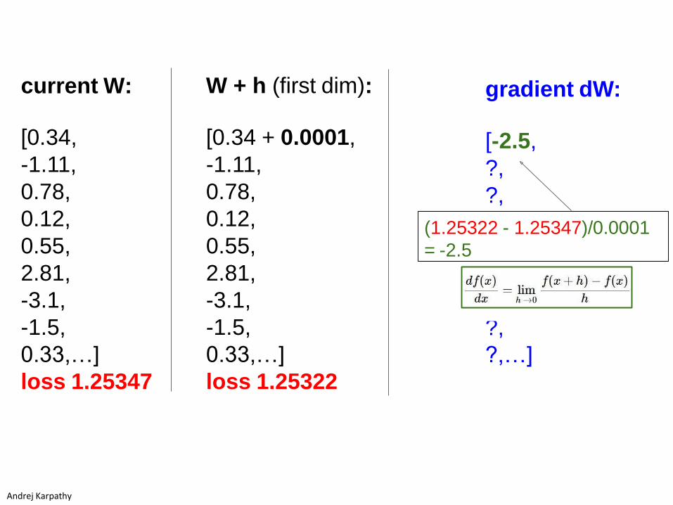
gradient dW:
[-2.5,
?,
?,
?,?,
?,
?,?,
?,…]
(1.25322 - 1.25347)/0.0001
= -2.5
current W:
[0.34,
-1.11,
0.78,
0.12,
0.55,
2.81,
-3.1,
-1.5,
0.33,…]
loss 1.25347
W + h (first dim):
[0.34 + 0.0001,
-1.11,
0.78,
0.12,
0.55,
2.81,
-3.1,
-1.5,
0.33,…]
loss 1.25322
Andrej Karpathy
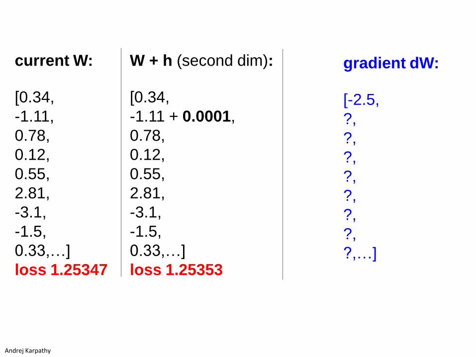
gradient dW:
[-2.5,
?,
?,
?,
?,
?,
?,
?,
?,…]
current W:
[0.34,
-1.11,
0.78,
0.12,
0.55,
2.81,
-3.1,
-1.5,
0.33,…]
loss 1.25347
W + h (second dim):
[0.34,
-1.11 + 0.0001,
0.78,
0.12,
0.55,
2.81,
-3.1,
-1.5,
0.33,…]
loss 1.25353
Andrej Karpathy
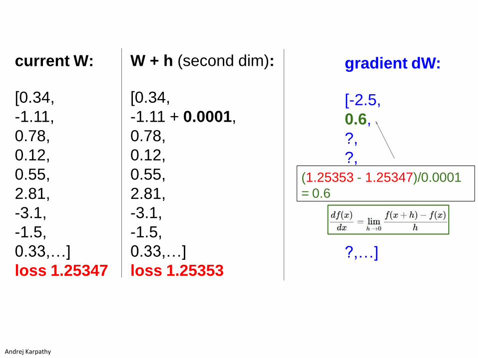
gradient dW:
[-2.5,
0.6,
?,
?,?,
?,
?,
?,
?,…]
current W:
[0.34,
-1.11,
0.78,
0.12,
0.55,
2.81,
-3.1,
-1.5,
0.33,…]
loss 1.25347
W + h (second dim):
[0.34,
-1.11 + 0.0001,
0.78,
0.12,
0.55,
2.81,
-3.1,
-1.5,
0.33,…]
loss 1.25353
(1.25353 - 1.25347)/0.0001
= 0.6
Andrej Karpathy
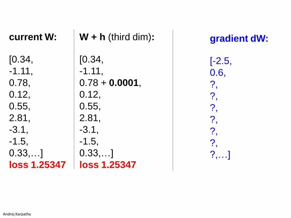
gradient dW:
[-2.5,
0.6,
?,
?,
?,
?,
?,
?,
?,…]
current W:
[0.34,
-1.11,
0.78,
0.12,
0.55,
2.81,
-3.1,
-1.5,
0.33,…]
loss 1.25347
W + h (third dim):
[0.34,
-1.11,
0.78 + 0.0001,
0.12,
0.55,
2.81,
-3.1,
-1.5,
0.33,…]
loss 1.25347
Andrej Karpathy
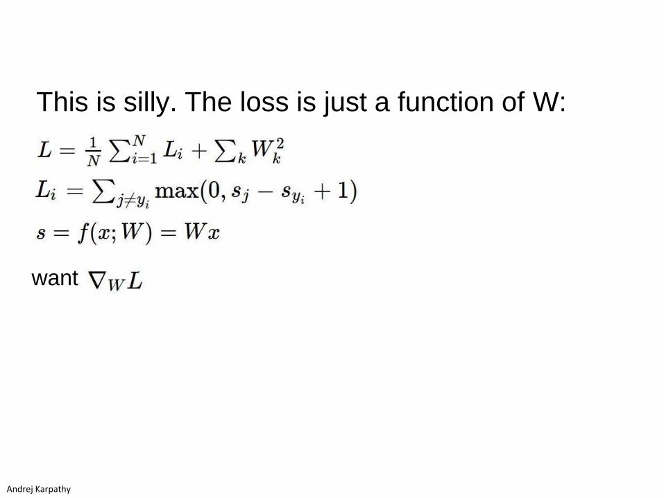
This is silly. The loss is just a function of W:
want
Andrej Karpathy
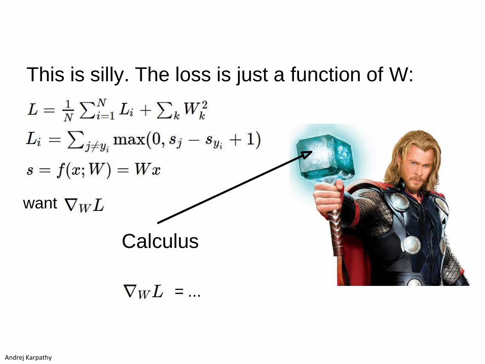
This is silly. The loss is just a function of W:
want
Calculus
= ...
Andrej Karpathy
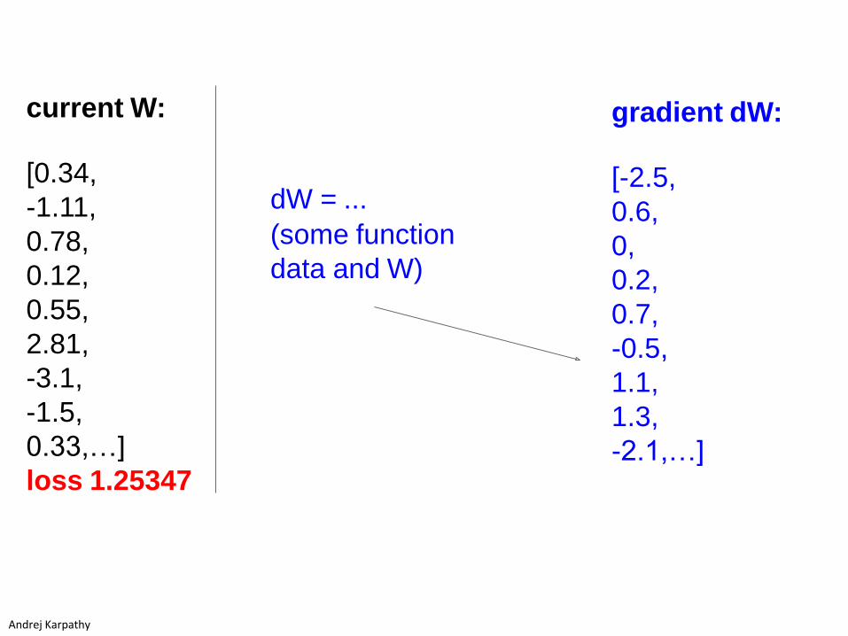
gradient dW:
[-2.5,
0.6,
0,
0.2,
0.7,
-0.5,
1.1,
1.3,
-2.1,…]
current W:
[0.34,
-1.11,
0.78,
0.12,
0.55,
2.81,
-3.1,
-1.5,
0.33,…]
loss 1.25347
dW = ...
(some function
data and W)
Andrej Karpathy
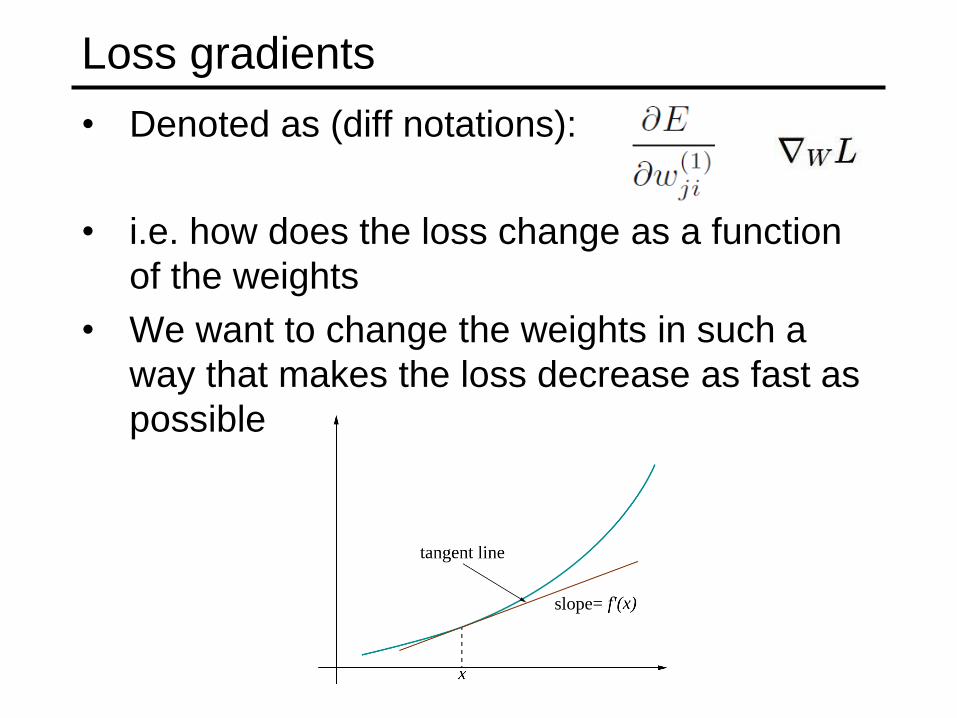
Loss gradients
• Denoted as (diff notations):
• i.e. how does the loss change as a function
of the weights
• We want to change the weights in such a
way that makes the loss decrease as fast as
possible
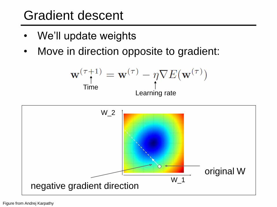
Gradient descent
• We’ll update weights
• Move in direction opposite to gradient:
L
Learning rateTime
Figure from Andrej Karpathy
original W
negative gradient directionW_1
W_2
Gradient descent
• Iteratively subtract the gradient with respect
to the model parameters (w)
• I.e. we’re moving in a direction opposite to
the gradient of the loss
• I.e. we’re moving towards smaller loss
Mini-batch gradient descent
• In classic gradient descent, we compute the
gradient from the loss for all training
examples
• Could also only use some of the data for
each gradient update
• We cycle through all the training examples
multiple times
• Each time we’ve cycled through all of them
once is called an ‘epoch’
• Allows faster training (e.g. on GPUs),
parallelization
Andrej Karpathy
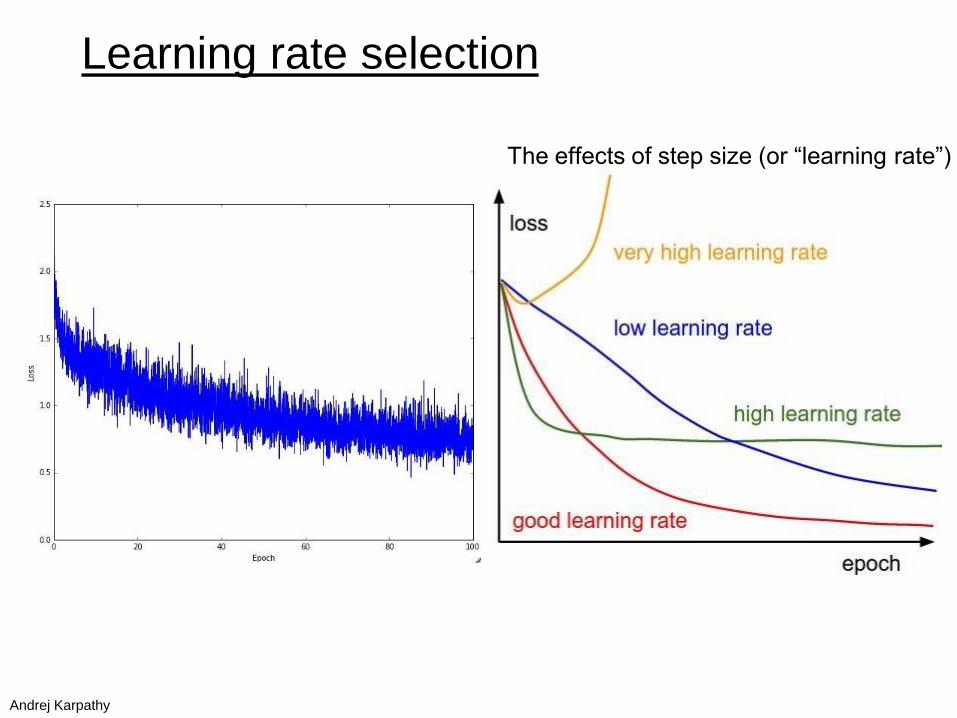
Learning rate selection
The effects of step size (or “learning rate”)
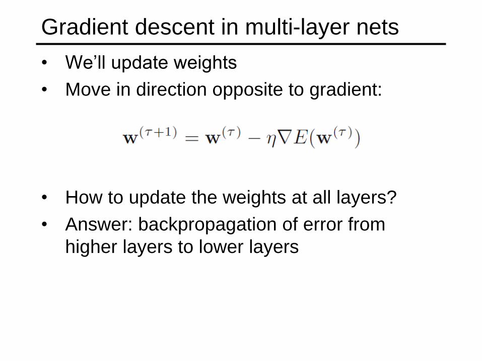
Gradient descent in multi-layer nets
• We’ll update weights
• Move in direction opposite to gradient:
• How to update the weights at all layers?
• Answer: backpropagation of error from
higher layers to lower layers
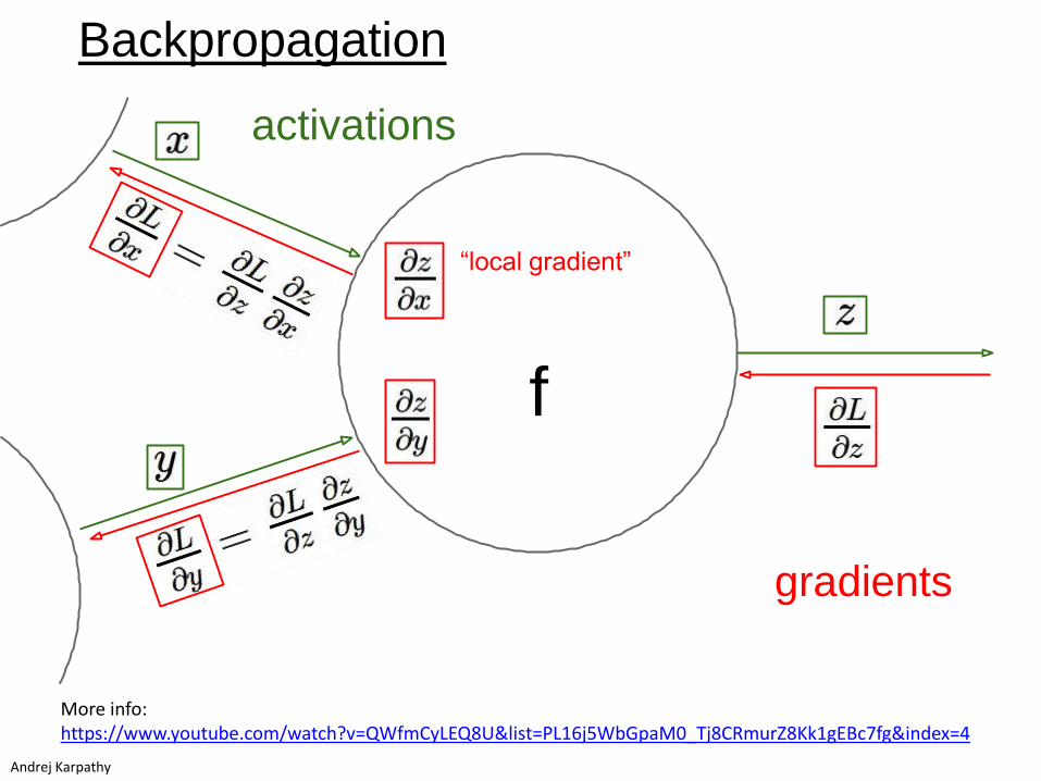
activations
“local gradient”
f
gradients
Andrej Karpathy
Backpropagation
More info:https://www.youtube.com/watch?v=QWfmCyLEQ8U&list=PL16j5WbGpaM0_Tj8CRmurZ8Kk1gEBc7fg&index=4
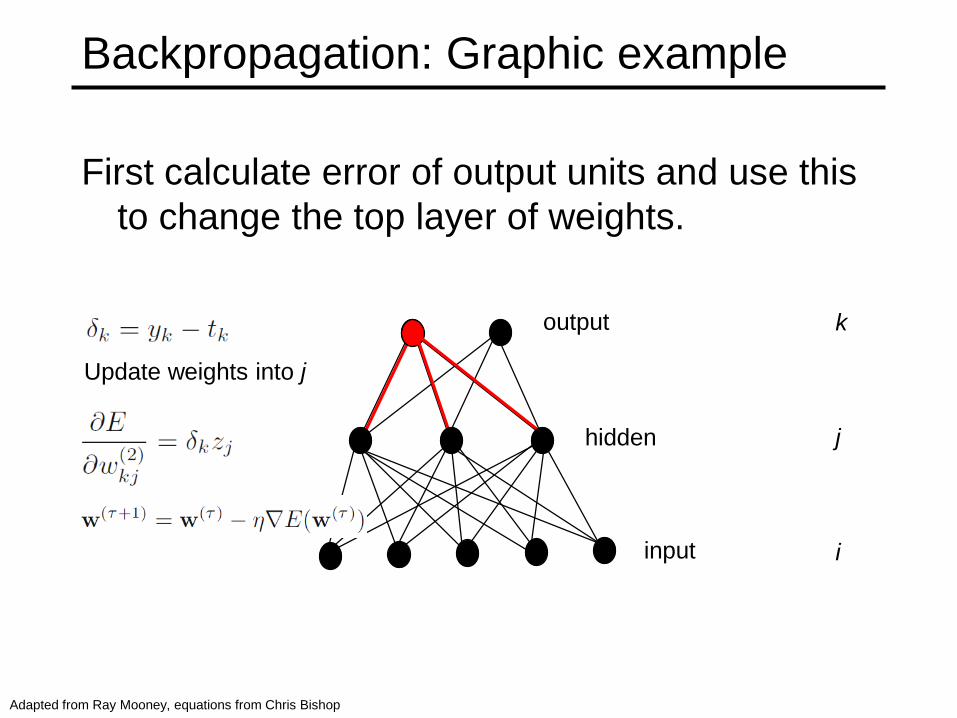
Backpropagation: Graphic example
First calculate error of output units and use this
to change the top layer of weights.
output
hidden
input
Update weights into j
Adapted from Ray Mooney, equations from Chris Bishop
k
j
i
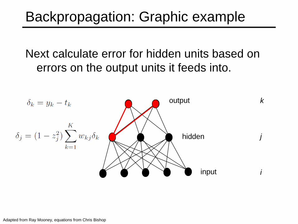
Backpropagation: Graphic example
Next calculate error for hidden units based on
errors on the output units it feeds into.
output
hidden
input
k
j
i
Adapted from Ray Mooney, equations from Chris Bishop
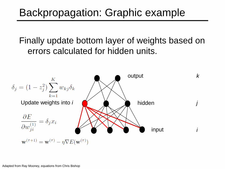
Backpropagation: Graphic example
Finally update bottom layer of weights based on
errors calculated for hidden units.
output
hidden
input
Update weights into i
k
j
i
Adapted from Ray Mooney, equations from Chris Bishop
Comments on training algorithm
• Not guaranteed to converge to zero training error, may
converge to local optima or oscillate indefinitely.
• However, in practice, does converge to low error for
many large networks on real data.
• Thousands of epochs (epoch = network sees all training
data once) may be required, hours or days to train.
• To avoid local-minima problems, run several trials
starting with different random weights (random restarts),
and take results of trial with lowest training set error.
• May be hard to set learning rate and to select number of
hidden units and layers.
• Neural networks had fallen out of fashion in 90s, early
2000s; back with a new name and significantly improved
performance (deep networks trained with dropout and
lots of data).
Ray Mooney, Carlos Guestrin, Dhruv Batra
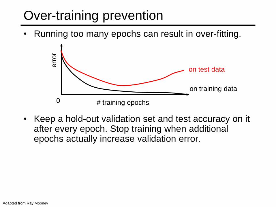
Over-training prevention
• Running too many epochs can result in over-fitting.
• Keep a hold-out validation set and test accuracy on it after every epoch. Stop training when additional epochs actually increase validation error.
0 # training epochs
err
or
on training data
on test data
Adapted from Ray Mooney
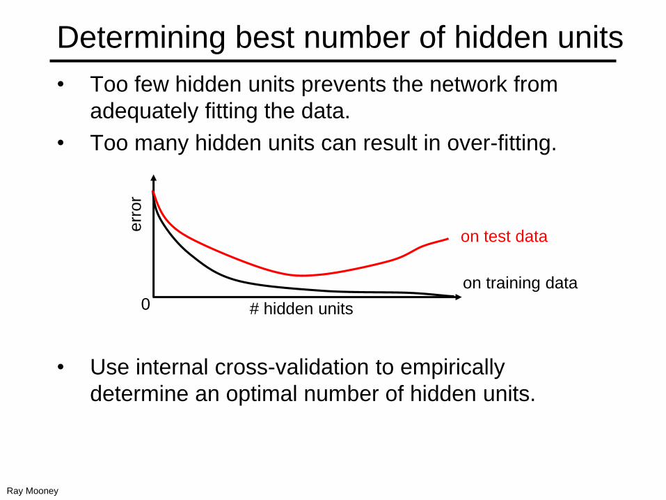
Determining best number of hidden units
• Too few hidden units prevents the network from
adequately fitting the data.
• Too many hidden units can result in over-fitting.
• Use internal cross-validation to empirically
determine an optimal number of hidden units.
err
or
on training data
on test data
0 # hidden units
Ray Mooney
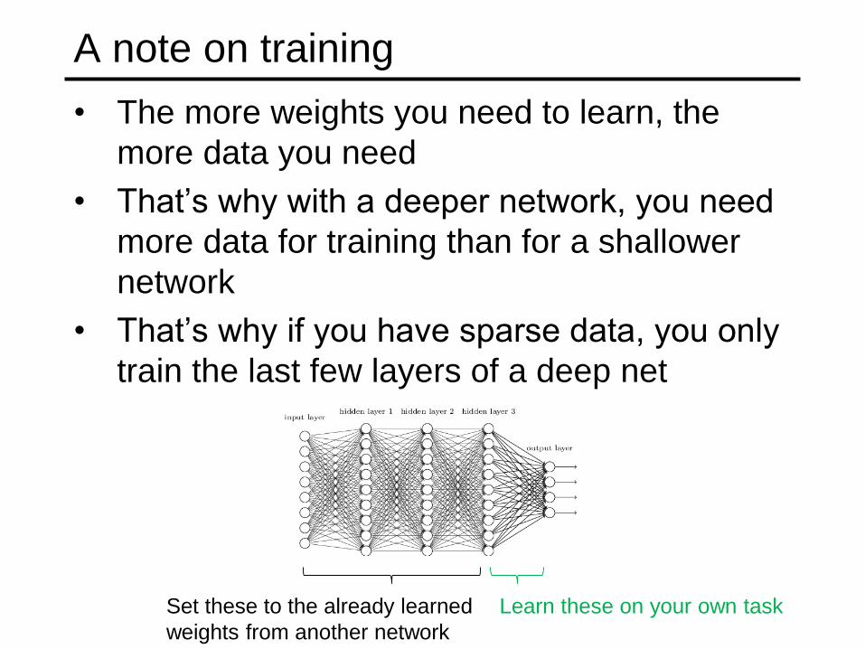
A note on training
• The more weights you need to learn, the
more data you need
• That’s why with a deeper network, you need
more data for training than for a shallower
network
• That’s why if you have sparse data, you only
train the last few layers of a deep net
Set these to the already learned
weights from another network
Learn these on your own task
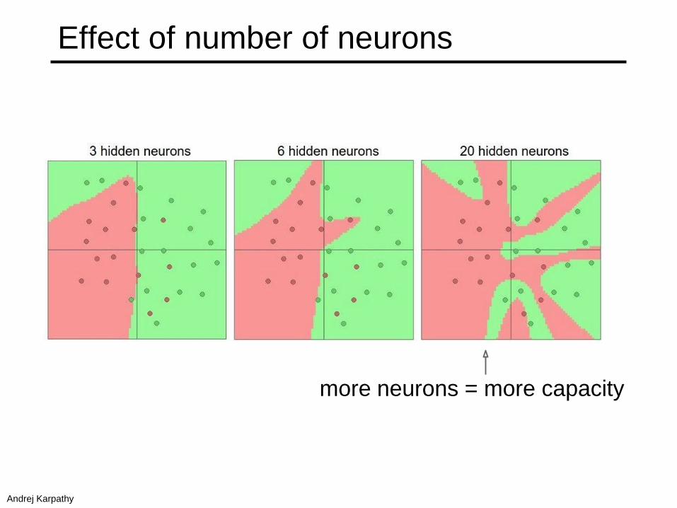
more neurons = more capacity
Effect of number of neurons
Andrej Karpathy
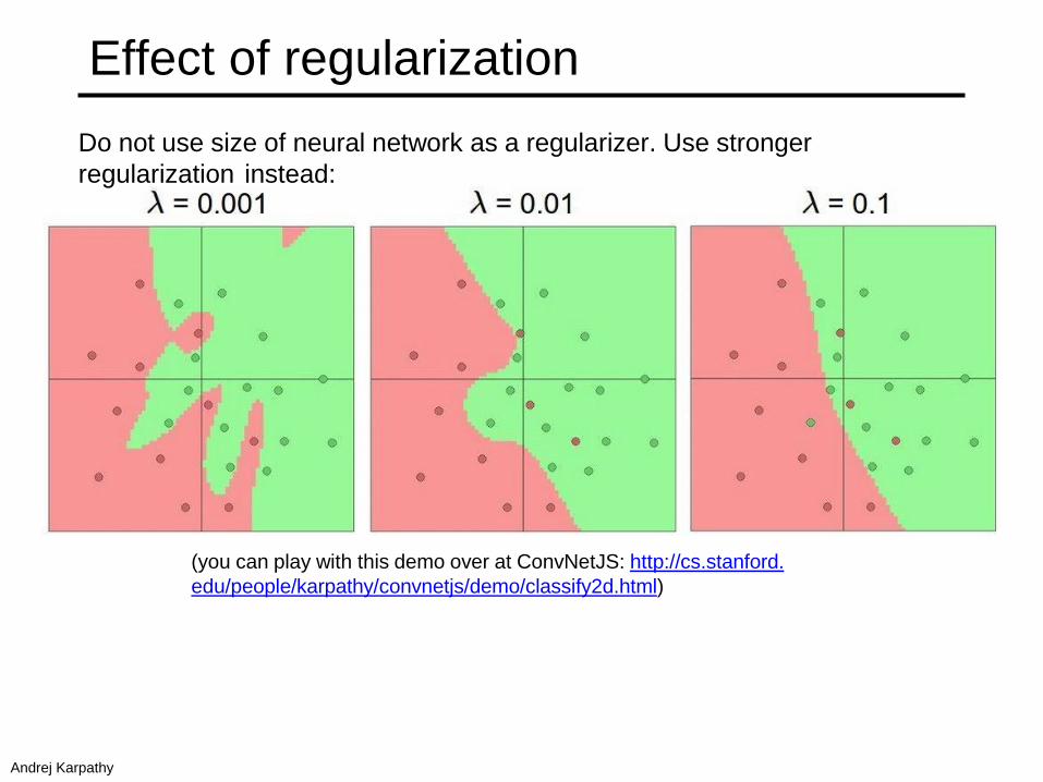
(you can play with this demo over at ConvNetJS: http://cs.stanford.
edu/people/karpathy/convnetjs/demo/classify2d.html)
Do not use size of neural network as a regularizer. Use stronger
regularization instead:
Effect of regularization
Andrej Karpathy
Hidden unit interpretation
• Trained hidden units can be seen as newly
constructed features that make the target concept
linearly separable in the transformed space.
• On many real domains, hidden units can be
interpreted as representing meaningful features
such as vowel detectors or edge detectors, etc.
• However, the hidden layer can also become a
distributed representation of the input in which each
individual unit is not easily interpretable as a
meaningful feature.
Ray Mooney
Summary
• We use deep neural networks because of
their strong performance in practice
• Feed-forward network architecture
• Training deep neural nets• We need an objective function that measures and guides us
towards good performance
• We need a way to minimize the loss function: stochastic
gradient descent
• We need backpropagation to propagate error towards all
layers and change weights at those layers
• Practices for preventing overfitting