Embed Size (px)
Citation preview

CS 147:Computer Systems Performance Analysis
Introduction to Queueing Theory
1 / 27
CS 147:Computer Systems Performance Analysis
Introduction to Queueing Theory
2015
-06-
15
CS147
Overview
Introduction and TerminologyPoisson Distributions
Fundamental ResultsStabilityLittle’s Law
M/M/*M/M/1M/M/mM/M/m/B
More General Queues
2 / 27
Overview
Introduction and TerminologyPoisson Distributions
Fundamental ResultsStabilityLittle’s Law
M/M/*M/M/1M/M/mM/M/m/B
More General Queues2015
-06-
15
CS147
Overview

Introduction and Terminology
What is a Queueing System?
I A queueing system is any system in which things arrive, hangaround for a while, and leave
I ExamplesI A bankI A freewayI A (computer) networkI A beehive
I The things that arrive and leave are customers or jobsI Customers leave after receiving serviceI Most queueing systems have (surprise!) a queue that can
store (delay) customers awaiting service
3 / 27
What is a Queueing System?
I A queueing system is any system in which things arrive, hangaround for a while, and leave
I ExamplesI A bankI A freewayI A (computer) networkI A beehive
I The things that arrive and leave are customers or jobsI Customers leave after receiving serviceI Most queueing systems have (surprise!) a queue that can
store (delay) customers awaiting service2015
-06-
15
CS147Introduction and Terminology
What is a Queueing System?
Introduction and Terminology
Parameters of a Queueing System
Arrival Process Injects customers into systemI Usually statisticalI Convenient to specify in terms of interarrival time
distributionI Most common is Poisson arrivals
Service Time Also statisticalNumber of Servers Often 1System Capacity Equals number of servers plus queue capacity.
Often assumed infinite for conveniencePopulation Maximum number of customers. Often assumed
infiniteService Discipline How next customer is chosen for service.
Often FCFS or priority
4 / 27
Parameters of a Queueing System
Arrival Process Injects customers into systemI Usually statisticalI Convenient to specify in terms of interarrival time
distributionI Most common is Poisson arrivals
Service Time Also statisticalNumber of Servers Often 1System Capacity Equals number of servers plus queue capacity.
Often assumed infinite for conveniencePopulation Maximum number of customers. Often assumed
infiniteService Discipline How next customer is chosen for service.
Often FCFS or priority
2015
-06-
15
CS147Introduction and Terminology
Parameters of a Queueing System
Introduction and Terminology
Arrival and Service Distributions
I Customer arrivals are random variablesI Next disk request from many processesI Next packet hitting GoogleI Next call to Chipotle
I Same is true for service timesI What distribution describes it?
I May be complicated (fractal, Zipf)I We often use Poisson for tractability
5 / 27
Arrival and Service Distributions
I Customer arrivals are random variablesI Next disk request from many processesI Next packet hitting GoogleI Next call to Chipotle
I Same is true for service timesI What distribution describes it?
I May be complicated (fractal, Zipf)I We often use Poisson for tractability
2015
-06-
15
CS147Introduction and Terminology
Arrival and Service Distributions
Introduction and Terminology Poisson Distributions
The Poisson Distribution
I Probability of exactly k arrivals in (0, t) is Pk (t) = (λt)keλt/k !I λ is arrival rate parameter
I More useful formulation is Poisson arrival distribution:I PDF A(t) = P[next arrival takes time ≤ t ] = 1− e−λt
I pdf a(t) = λe−λt
I Also known as exponential or memoryless distributionI Mean = standard deviation = λ
I Poisson distribution is memorylessI Assume P[arrival within 1 second] at time t0 = xI Then P[arrival within 1 second] at time t1 > t0 is also x
I I.e., no memory that time has passedI Often true in real world
I E.g., when I go to Von’s doesn’t affect when you go
6 / 27
The Poisson Distribution
I Probability of exactly k arrivals in (0, t) is Pk (t) = (λt)keλt/k !I λ is arrival rate parameter
I More useful formulation is Poisson arrival distribution:I PDF A(t) = P[next arrival takes time ≤ t ] = 1− e−λt
I pdf a(t) = λe−λt
I Also known as exponential or memoryless distributionI Mean = standard deviation = λ
I Poisson distribution is memorylessI Assume P[arrival within 1 second] at time t0 = xI Then P[arrival within 1 second] at time t1 > t0 is also x
I I.e., no memory that time has passedI Often true in real world
I E.g., when I go to Von’s doesn’t affect when you go2015
-06-
15
CS147Introduction and Terminology
Poisson DistributionsThe Poisson Distribution

Introduction and Terminology Poisson Distributions
Splitting and Merging Poisson Processes
I Merging streams of Poisson events (e.g., arrivals) is Poisson
λ =k∑
i=1
λi
I Splitting a Poisson stream randomly gives Poisson streams; ifstream i has probability pi , then
λi = piλ
7 / 27
Splitting and Merging Poisson Processes
I Merging streams of Poisson events (e.g., arrivals) is Poisson
λ =k∑
i=1
λi
I Splitting a Poisson stream randomly gives Poisson streams; ifstream i has probability pi , then
λi = piλ
2015
-06-
15
CS147Introduction and Terminology
Poisson DistributionsSplitting and Merging Poisson Processes
Introduction and Terminology Poisson Distributions
Kendall’s Notation
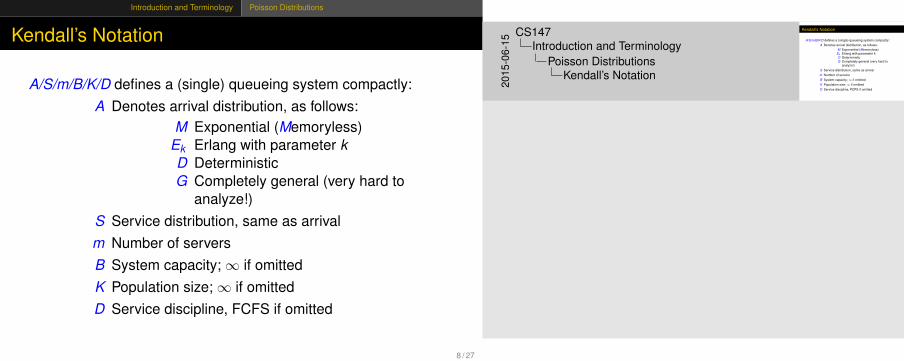
A/S/m/B/K/D defines a (single) queueing system compactly:A Denotes arrival distribution, as follows:
M Exponential (Memoryless)Ek Erlang with parameter kD DeterministicG Completely general (very hard to
analyze!)S Service distribution, same as arrivalm Number of serversB System capacity;∞ if omittedK Population size;∞ if omittedD Service discipline, FCFS if omitted
8 / 27
Kendall’s Notation
A/S/m/B/K/D defines a (single) queueing system compactly:A Denotes arrival distribution, as follows:
M Exponential (Memoryless)Ek Erlang with parameter kD DeterministicG Completely general (very hard to
analyze!)S Service distribution, same as arrivalm Number of serversB System capacity;∞ if omittedK Population size;∞ if omittedD Service discipline, FCFS if omitted
2015
-06-
15
CS147Introduction and Terminology
Poisson DistributionsKendall’s Notation
Introduction and Terminology Poisson Distributions
Examples of Kendall’s Notation
D/D/1 Arrivals on clock tick, fixed service times, one serverM/M/m Memoryless arrivals, memoryless service, multiple
servers (good model of a bank)M/M/m/m Customers go away rather than wait in line
G/G/1 Modern disk drive
9 / 27
Examples of Kendall’s Notation
D/D/1 Arrivals on clock tick, fixed service times, one serverM/M/m Memoryless arrivals, memoryless service, multiple
servers (good model of a bank)M/M/m/m Customers go away rather than wait in line
G/G/1 Modern disk drive
2015
-06-
15
CS147Introduction and Terminology
Poisson DistributionsExamples of Kendall’s Notation
Introduction and Terminology Poisson Distributions
Common Variables
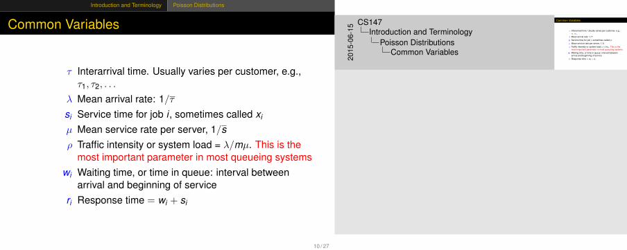
τ Interarrival time. Usually varies per customer, e.g.,τ1, τ2, . . .
λ Mean arrival rate: 1/τsi Service time for job i , sometimes called xi
µ Mean service rate per server, 1/sρ Traffic intensity or system load = λ/mµ. This is the
most important parameter in most queueing systemswi Waiting time, or time in queue: interval between
arrival and beginning of serviceri Response time = wi + si
10 / 27
Common Variables
τ Interarrival time. Usually varies per customer, e.g.,τ1, τ2, . . .
λ Mean arrival rate: 1/τsi Service time for job i , sometimes called xi
µ Mean service rate per server, 1/sρ Traffic intensity or system load = λ/mµ. This is the
most important parameter in most queueing systemswi Waiting time, or time in queue: interval between
arrival and beginning of serviceri Response time = wi + si20
15-0
6-15
CS147Introduction and Terminology
Poisson DistributionsCommon Variables
Fundamental Results Stability
Stability
I A system is stable iff λ < mµ ≡ ρ < 1I Otherwise, system can’t keep up and queue grows to∞I Exception: in D/D/m, ρ = 1 is OK
11 / 27
Stability
I A system is stable iff λ < mµ ≡ ρ < 1I Otherwise, system can’t keep up and queue grows to∞I Exception: in D/D/m, ρ = 1 is OK
2015
-06-
15
CS147Fundamental Results
StabilityStability
Fundamental Results Little’s Law
Little’s Law
I Let n = Number of jobs in systemI Then n = λrI Likewise, if nq = Number of jobs in queue, then nq = λwI True regardless of distributions, queueing disciplines, etc., as
long as system is in equilibriumI May seem obvious:
I If ten people are ahead of you in line, and each takes about 1minute for service, you’re going to be stuck there for 10minutes
I Not proved until 1961I Often useful for calculating queue lengths:
I Packet takes 2s to arrive, you’re sending 100 pps⇒ Mean queue length = 100 pkt/s× 2s = 200 pkts
12 / 27
Little’s Law
I Let n = Number of jobs in systemI Then n = λrI Likewise, if nq = Number of jobs in queue, then nq = λwI True regardless of distributions, queueing disciplines, etc., as
long as system is in equilibriumI May seem obvious:
I If ten people are ahead of you in line, and each takes about 1minute for service, you’re going to be stuck there for 10minutes
I Not proved until 1961I Often useful for calculating queue lengths:
I Packet takes 2s to arrive, you’re sending 100 pps⇒ Mean queue length = 100 pkt/s× 2s = 200 pkts
2015
-06-
15
CS147Fundamental Results
Little’s LawLittle’s Law
Fundamental Results Little’s Law
Deriving Little’s Law
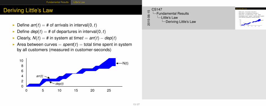
I Define arr(t) = # of arrivals in interval(0, t)I Define dep(t) = # of departures in interval(0, t)I Clearly, N(t) = # in system at timet = arr(t)− dep(t)I Area between curves = spent(t) = total time spent in system
by all customers (measured in customer-seconds)
0 5 10 15 20 25
0
2
4
6
8
10N(t)
arr(t)
dep(t)
13 / 27
Deriving Little’s Law
I Define arr(t) = # of arrivals in interval(0, t)I Define dep(t) = # of departures in interval(0, t)I Clearly, N(t) = # in system at timet = arr(t)− dep(t)I Area between curves = spent(t) = total time spent in system
by all customers (measured in customer-seconds)
0 5 10 15 20 25
0
2
4
6
8
10N(t)
arr(t)
dep(t)2015
-06-
15
CS147Fundamental Results
Little’s LawDeriving Little’s Law
Fundamental Results Little’s Law
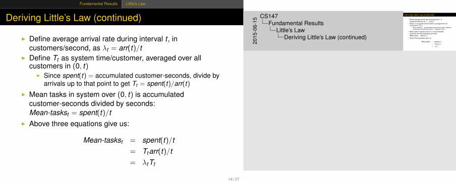
Deriving Little’s Law (continued)
I Define average arrival rate during interval t , incustomers/second, as λt = arr(t)/t
I Define Tt as system time/customer, averaged over allcustomers in (0, t)
I Since spent(t) = accumulated customer-seconds, divide byarrivals up to that point to get Tt = spent(t)/arr(t)
I Mean tasks in system over (0, t) is accumulatedcustomer-seconds divided by seconds:Mean-taskst = spent(t)/t
I Above three equations give us:
Mean-taskst = spent(t)/t= Ttarr(t)/t= λtTt
14 / 27
Deriving Little’s Law (continued)
I Define average arrival rate during interval t , incustomers/second, as λt = arr(t)/t
I Define Tt as system time/customer, averaged over allcustomers in (0, t)
I Since spent(t) = accumulated customer-seconds, divide byarrivals up to that point to get Tt = spent(t)/arr(t)
I Mean tasks in system over (0, t) is accumulatedcustomer-seconds divided by seconds:Mean-taskst = spent(t)/t
I Above three equations give us:
Mean-taskst = spent(t)/t= Ttarr(t)/t= λtTt
2015
-06-
15
CS147Fundamental Results
Little’s LawDeriving Little’s Law (continued)
Fundamental Results Little’s Law
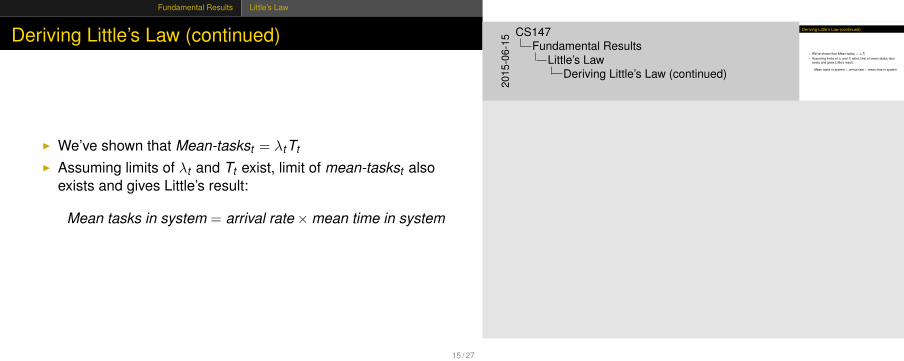
Deriving Little’s Law (continued)
I We’ve shown that Mean-taskst = λtTt
I Assuming limits of λt and Tt exist, limit of mean-taskst alsoexists and gives Little’s result:
Mean tasks in system = arrival rate×mean time in system
15 / 27
Deriving Little’s Law (continued)
I We’ve shown that Mean-taskst = λtTt
I Assuming limits of λt and Tt exist, limit of mean-taskst alsoexists and gives Little’s result:
Mean tasks in system = arrival rate×mean time in system
2015
-06-
15
CS147Fundamental Results
Little’s LawDeriving Little’s Law (continued)
M/M/* M/M/1
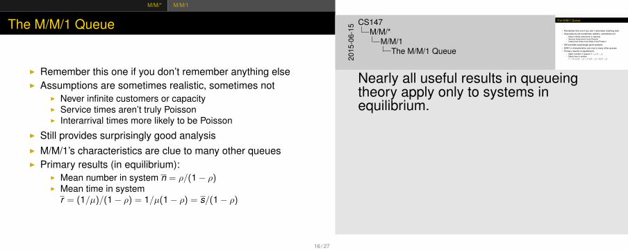
The M/M/1 Queue
I Remember this one if you don’t remember anything elseI Assumptions are sometimes realistic, sometimes not
I Never infinite customers or capacityI Service times aren’t truly PoissonI Interarrival times more likely to be Poisson
I Still provides surprisingly good analysisI M/M/1’s characteristics are clue to many other queuesI Primary results (in equilibrium):
I Mean number in system n = ρ/(1− ρ)I Mean time in system
r = (1/µ)/(1− ρ) = 1/µ(1− ρ) = s/(1− ρ)
16 / 27
The M/M/1 Queue
I Remember this one if you don’t remember anything elseI Assumptions are sometimes realistic, sometimes not
I Never infinite customers or capacityI Service times aren’t truly PoissonI Interarrival times more likely to be Poisson
I Still provides surprisingly good analysisI M/M/1’s characteristics are clue to many other queuesI Primary results (in equilibrium):
I Mean number in system n = ρ/(1− ρ)I Mean time in system
r = (1/µ)/(1− ρ) = 1/µ(1− ρ) = s/(1− ρ)2015
-06-
15
CS147M/M/*
M/M/1The M/M/1 Queue
Nearly all useful results in queueingtheory apply only to systems inequilibrium.
M/M/* M/M/1
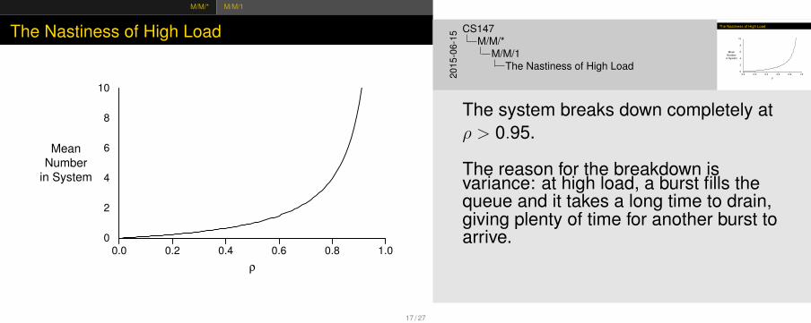
The Nastiness of High Load
0.0 0.2 0.4 0.6 0.8 1.0
ρ
0
2
4
6
8
10
Mean
Number
in System
17 / 27
The Nastiness of High Load
0.0 0.2 0.4 0.6 0.8 1.0
ρ
0
2
4
6
8
10
Mean
Number
in System
2015
-06-
15
CS147M/M/*
M/M/1The Nastiness of High Load
The system breaks down completely atρ > 0.95.
The reason for the breakdown isvariance: at high load, a burst fills thequeue and it takes a long time to drain,giving plenty of time for another burst toarrive.
M/M/* M/M/1
More M/M/1 Results
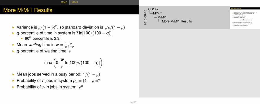
I Variance is ρ/(1− ρ)2, so standard deviation is√ρ/(1− ρ)
I q-percentile of time in system is r ln[100/(100− q)]I 90th percentile is 2.3r
I Mean waiting time is w = 1µ
ρ1−ρ
I q-percentile of waiting time is
max(
0,wρ
ln[100ρ/(100− q)])
I Mean jobs served in a busy period: 1/(1− ρ)I Probability of n jobs in system pn = (1− ρ)ρn
I Probability of > n jobs in system: ρn
18 / 27
More M/M/1 Results
I Variance is ρ/(1− ρ)2, so standard deviation is√ρ/(1− ρ)
I q-percentile of time in system is r ln[100/(100− q)]I 90th percentile is 2.3r
I Mean waiting time is w = 1µ
ρ1−ρ
I q-percentile of waiting time is
max(
0,wρ
ln[100ρ/(100− q)])
I Mean jobs served in a busy period: 1/(1− ρ)I Probability of n jobs in system pn = (1− ρ)ρn
I Probability of > n jobs in system: ρn2015
-06-
15
CS147M/M/*
M/M/1More M/M/1 Results
M/M/* M/M/1
M/M/1 Example
I Web server gets 1200 requests/hour w/ Poisson arrivalsI Typical request takes 1s to serveI ρ = 1200/3600 = 0.33I Mean requests in service = 0.33/0.67 = 0.5I Mean response time r = (1/1)/(1− 0.33) = 1.5sI 90th percentile response time = 3.4s
I But if Slashdot hits. . .
19 / 27
M/M/1 Example
I Web server gets 1200 requests/hour w/ Poisson arrivalsI Typical request takes 1s to serveI ρ = 1200/3600 = 0.33I Mean requests in service = 0.33/0.67 = 0.5I Mean response time r = (1/1)/(1− 0.33) = 1.5sI 90th percentile response time = 3.4s
I But if Slashdot hits. . .
2015
-06-
15
CS147M/M/*
M/M/1M/M/1 Example
This slide has animations.
M/M/* M/M/1
M/M/1 Example
I Web server gets 1200 requests/hour w/ Poisson arrivalsI Typical request takes 1s to serveI ρ = 1200/3600 = 0.33I Mean requests in service = 0.33/0.67 = 0.5I Mean response time r = (1/1)/(1− 0.33) = 1.5sI 90th percentile response time = 3.4sI But if Slashdot hits. . .
19 / 27
M/M/1 Example
I Web server gets 1200 requests/hour w/ Poisson arrivalsI Typical request takes 1s to serveI ρ = 1200/3600 = 0.33I Mean requests in service = 0.33/0.67 = 0.5I Mean response time r = (1/1)/(1− 0.33) = 1.5sI 90th percentile response time = 3.4sI But if Slashdot hits. . .
2015
-06-
15
CS147M/M/*
M/M/1M/M/1 Example
This slide has animations.
M/M/* M/M/1
M/M/1 Example (cont’d)
I Suppose Slashdot raises request rate to 3500/hrI Now ρ = 3500/3600 = 0.972I Mean requests in service = 0.972/(1− 0.972) = 34.7I r = 1/0.028 = 35.7 secondsI 90th percentile response time = 82.8s
I And don’t even think about 4000 requests/hr
20 / 27
M/M/1 Example (cont’d)
I Suppose Slashdot raises request rate to 3500/hrI Now ρ = 3500/3600 = 0.972I Mean requests in service = 0.972/(1− 0.972) = 34.7I r = 1/0.028 = 35.7 secondsI 90th percentile response time = 82.8s
I And don’t even think about 4000 requests/hr
2015
-06-
15
CS147M/M/*
M/M/1M/M/1 Example (cont’d)
This slide has animations.
M/M/* M/M/1
M/M/1 Example (cont’d)
I Suppose Slashdot raises request rate to 3500/hrI Now ρ = 3500/3600 = 0.972I Mean requests in service = 0.972/(1− 0.972) = 34.7I r = 1/0.028 = 35.7 secondsI 90th percentile response time = 82.8sI And don’t even think about 4000 requests/hr
20 / 27
M/M/1 Example (cont’d)
I Suppose Slashdot raises request rate to 3500/hrI Now ρ = 3500/3600 = 0.972I Mean requests in service = 0.972/(1− 0.972) = 34.7I r = 1/0.028 = 35.7 secondsI 90th percentile response time = 82.8sI And don’t even think about 4000 requests/hr
2015
-06-
15
CS147M/M/*
M/M/1M/M/1 Example (cont’d)
This slide has animations.
M/M/* M/M/m
M/M/m
I Multiple servers, one queueI ρ = λ/(mµ)I We’ll need probability of empty system:
p0 =1
(mρ)m
m!(1− ρ)+
m−1∑k=0
(mρ)k
k !
I Probability of queueing:
% = P(≥ m jobs) =(mρ)m
m!(1− ρ)p0
21 / 27
M/M/m
I Multiple servers, one queueI ρ = λ/(mµ)I We’ll need probability of empty system:
p0 =1
(mρ)m
m!(1− ρ)+
m−1∑k=0
(mρ)k
k !
I Probability of queueing:
% = P(≥ m jobs) =(mρ)m
m!(1− ρ)p020
15-0
6-15
CS147M/M/*
M/M/mM/M/m
For m = 1, % = ρ
M/M/* M/M/m
M/M/m (cont’d)
I Mean jobs in system: n = mρ+ ρ%/(1− ρ)I Mean time in system:
r =1µ
(1 +
%
m(1− ρ)
)I Mean waiting time: w = %/[mµ(1− ρ)]I q-percentile of waiting time:
max(
0,w%
ln100%
100− q
)
22 / 27
M/M/m (cont’d)
I Mean jobs in system: n = mρ+ ρ%/(1− ρ)I Mean time in system:
r =1µ
(1 +
%
m(1− ρ)
)I Mean waiting time: w = %/[mµ(1− ρ)]I q-percentile of waiting time:
max(
0,w%
ln100%
100− q
)
2015
-06-
15
CS147M/M/*
M/M/mM/M/m (cont’d)
M/M/* M/M/m
m×M/M/1 vs. M/M/m
I For m separate M/M/1 queues, each queue sees arrival rateof λM/M/1 = λ/m
I But ρ is unchanged
I rm×M/M/1 = 1µ
(1
1−ρ
)?> rM/M/m = 1
µ
(1 + %
m(1−ρ)
)I 1
?> 1− ρ+ %
m
I ρ?> p0
(mρ)m
m!m(1−ρ)
I 1?> p0
(mρ)m−1
m!(1−ρ)
I 1?>
(1
(mρ)mm!(1−ρ)+
∑m−1k=0
(mρ)kk!
)(mρ)m−1
m!(1−ρ)
I (mρ)m
m!(1−ρ) +∑m−1
k=0(mρ)k
k! > (mρ)m−1
m!(1−ρ)
23 / 27
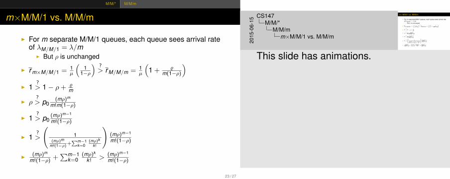
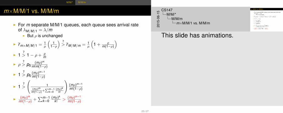
m×M/M/1 vs. M/M/m
I For m separate M/M/1 queues, each queue sees arrival rateof λM/M/1 = λ/m
I But ρ is unchanged
I rm×M/M/1 = 1µ
(1
1−ρ
)?> rM/M/m = 1
µ
(1 + %
m(1−ρ)
)I 1
?> 1− ρ+ %
m
I ρ?> p0
(mρ)m
m!m(1−ρ)
I 1?> p0
(mρ)m−1
m!(1−ρ)
I 1?>
(1
(mρ)mm!(1−ρ)+
∑m−1k=0
(mρ)kk!
)(mρ)m−1
m!(1−ρ)
I (mρ)m
m!(1−ρ) +∑m−1
k=0(mρ)k
k! > (mρ)m−1
m!(1−ρ)
2015
-06-
15
CS147M/M/*
M/M/mm×M/M/1 vs. M/M/m
This slide has animations.
M/M/* M/M/m
m×M/M/1 vs. M/M/m
I For m separate M/M/1 queues, each queue sees arrival rateof λM/M/1 = λ/m
I But ρ is unchanged
I rm×M/M/1 = 1µ
(1
1−ρ
)?> rM/M/m = 1
µ
(1 + %
m(1−ρ)
)I 1
?> 1− ρ+ %
m
I ρ?> p0
(mρ)m
m!m(1−ρ)
I 1?> p0
(mρ)m−1
m!(1−ρ)
I 1?>
(1
(mρ)mm!(1−ρ)+
∑m−1k=0
(mρ)kk!
)(mρ)m−1
m!(1−ρ)
I (mρ)m
m!(1−ρ) +∑m−1
k=0(mρ)k
k! > (mρ)m−1
m!(1−ρ)
23 / 27
m×M/M/1 vs. M/M/m
I For m separate M/M/1 queues, each queue sees arrival rateof λM/M/1 = λ/m
I But ρ is unchanged
I rm×M/M/1 = 1µ
(1
1−ρ
)?> rM/M/m = 1
µ
(1 + %
m(1−ρ)
)I 1
?> 1− ρ+ %
m
I ρ?> p0
(mρ)m
m!m(1−ρ)
I 1?> p0
(mρ)m−1
m!(1−ρ)
I 1?>
(1
(mρ)mm!(1−ρ)+
∑m−1k=0
(mρ)kk!
)(mρ)m−1
m!(1−ρ)
I (mρ)m
m!(1−ρ) +∑m−1
k=0(mρ)k
k! > (mρ)m−1
m!(1−ρ)
2015
-06-
15
CS147M/M/*
M/M/mm×M/M/1 vs. M/M/m
This slide has animations.
M/M/* M/M/m
Running Some Numbers
I Assume 5 servers, ρ = 0.5, µ = 1I Then rm×M/M/1 = 1/(1− ρ) = 2
I % = (mρ)m
m!(1−ρ)p0 = (2.5)5
5!(0.5)p0 = 97.760 p0 = 1.63p0
I p0 = 1(mρ)m
m!(1−ρ)+∑m−1
k=0(mρ)k
k!
= 11.63+1+ 2.51
1 + 2.522 + 2.53
3! + 2.544!
I p0 = 11.63+1+2.5+3.13+2.60+1.63 = 1
12.49 = 0.08I So % = 1.63(0.08) = 0.13I And rm/M/m = 1 + %
m(1−ρ) = 1 + 0.135(1−0.5) = 1 + 0.13
2.5 = 1.05I In terms of previous slide’s inequality,
97.760 +1+2.5+3.13+2.60+1.63 = 12.49 > 2.54
5!(0.5) =39.160 = 0.65
24 / 27
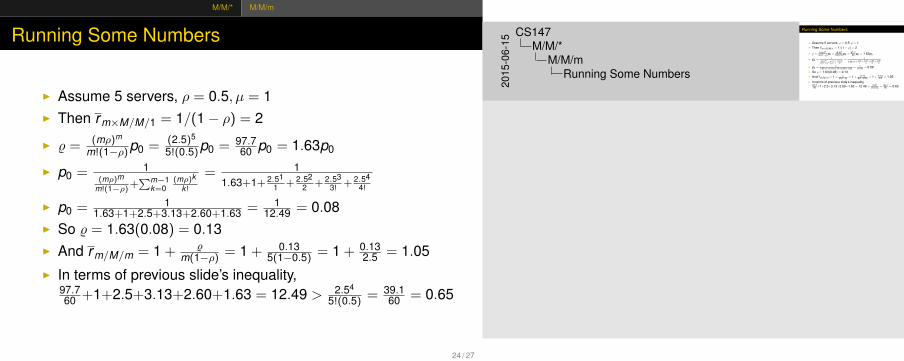
Running Some Numbers
I Assume 5 servers, ρ = 0.5, µ = 1I Then rm×M/M/1 = 1/(1− ρ) = 2
I % = (mρ)m
m!(1−ρ)p0 = (2.5)5
5!(0.5)p0 = 97.760 p0 = 1.63p0
I p0 = 1(mρ)m
m!(1−ρ)+∑m−1
k=0(mρ)k
k!
= 11.63+1+ 2.51
1 + 2.522 + 2.53
3! + 2.544!
I p0 = 11.63+1+2.5+3.13+2.60+1.63 = 1
12.49 = 0.08I So % = 1.63(0.08) = 0.13I And rm/M/m = 1 + %
m(1−ρ) = 1 + 0.135(1−0.5) = 1 + 0.13
2.5 = 1.05I In terms of previous slide’s inequality,
97.760 +1+2.5+3.13+2.60+1.63 = 12.49 > 2.54
5!(0.5) =39.160 = 0.6520
15-0
6-15
CS147M/M/*
M/M/mRunning Some Numbers
M/M/* M/M/m
m×M/M/1 vs. M/M/m (cont’d)
I A similar result holds for varianceI Conclusion: single queue, multiple server is always better
than one queue per serverI Question 1: When is this false? (hint: multiple cores)I Question 2: Why do so many movie theaters have multiple
lines for popcorn?
25 / 27
m×M/M/1 vs. M/M/m (cont’d)
I A similar result holds for varianceI Conclusion: single queue, multiple server is always better
than one queue per serverI Question 1: When is this false? (hint: multiple cores)I Question 2: Why do so many movie theaters have multiple
lines for popcorn?
2015
-06-
15
CS147M/M/*
M/M/mm×M/M/1 vs. M/M/m (cont’d)
M/M/* M/M/m/B
M/M/m/B
I Real systems have finite capacityI Previous analysis applies only under light loads (relative to
capacity)I Considering limit has several effects:
I Lost jobs (obviously)I Loss rate pB becomes important parameterI Mean response time drops compared to M/M/m/∞ (Why?)
26 / 27
M/M/m/B
I Real systems have finite capacityI Previous analysis applies only under light loads (relative to
capacity)I Considering limit has several effects:
I Lost jobs (obviously)I Loss rate pB becomes important parameterI Mean response time drops compared to M/M/m/∞ (Why?)
2015
-06-
15
CS147M/M/*
M/M/m/BM/M/m/B

More General Queues
Extending the Results
I Unsurprisingly, generality equates to (mathematical)complexity
I Many special cases have been analyzed (e.g., Erlangdistributions)
I Little’s Law always appliesI Important cases:
I M/G/1I M/D/1I G/G/m (but mostly intractable)
27 / 27
Extending the Results
I Unsurprisingly, generality equates to (mathematical)complexity
I Many special cases have been analyzed (e.g., Erlangdistributions)
I Little’s Law always appliesI Important cases:
I M/G/1I M/D/1I G/G/m (but mostly intractable)20
15-0
6-15
CS147More General Queues
Extending the Results