Embed Size (px)
Citation preview
SegmentationCS 4495 Computer Vision – A. Bobick
Aaron Bobick (slides by Tucker Hermans)School of Interactive Computing
CS 4495 Computer Vision
Segmentation

SegmentationCS 4495 Computer Vision – A. Bobick
Administrivia• PS 4: Out but I was a bit late so due date pushed back to
Oct 29.
• OpenCV now has real SIFT again (the “notfree” packages). If using Python and OpenCV you should be able to use those calls.
• We’re still investigating SIFT for Python for those *not* using OpenCV.
SegmentationCS 4495 Computer Vision – A. Bobick
Why segmentation?

SegmentationCS 4495 Computer Vision – A. Bobick
Segmentation of Coherent Regions
Berkeley segmentation database:http://www.eecs.berkeley.edu/Research/Projects/CS/vision/grouping/segbench/
Slide by Svetlana Lazebnik
SegmentationCS 4495 Computer Vision – A. Bobick
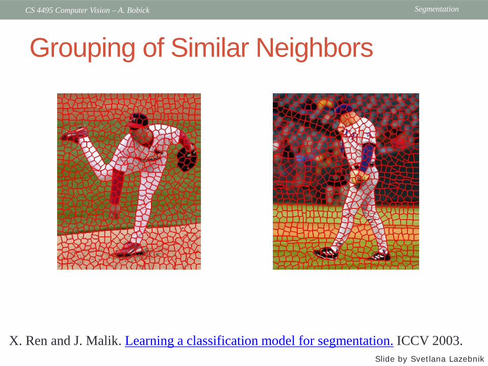
Grouping of Similar Neighbors
X. Ren and J. Malik. Learning a classification model for segmentation. ICCV 2003.Slide by Svetlana Lazebnik

SegmentationCS 4495 Computer Vision – A. Bobick
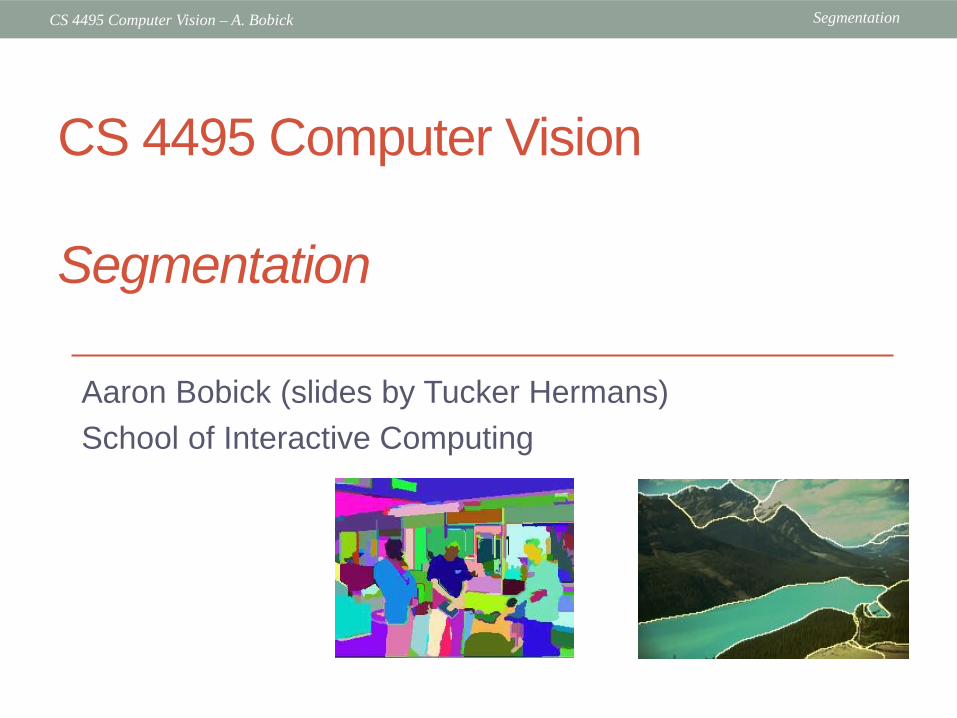
Figure Ground Segmentation• Separate the foreground object (figure) from the
background (ground)
D. Tsai, M. Flagg, and J. M. Rehg. “Motion Coherent Tracking with Multi-label MRF optimization.” BMVC 2010.
SegmentationCS 4495 Computer Vision – A. Bobick
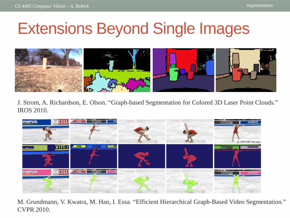
Extensions Beyond Single Images
M. Grundmann, V. Kwatra, M. Han, I. Essa. “Efficient Hierarchical Graph-Based Video Segmentation.” CVPR 2010.
J. Strom, A. Richardson, E. Olson. “Graph-based Segmentation for Colored 3D Laser Point Clouds.” IROS 2010.

SegmentationCS 4495 Computer Vision – A. Bobick
intensity
pixe
l cou
nt
input image
black pixels gray pixels
white pixels
• These intensities define the three groups.• We could label every pixel in the image according to
which of these primary intensities it is.• i.e., segment the image based on the intensity feature.
• What if the image isn’t quite so simple?
1 23
Kristen Grauman
Image segmentation: toy example

SegmentationCS 4495 Computer Vision – A. Bobick
intensity
pixe
l cou
nt
input image
input image intensity
pixe
l cou
nt
Kristen Grauman
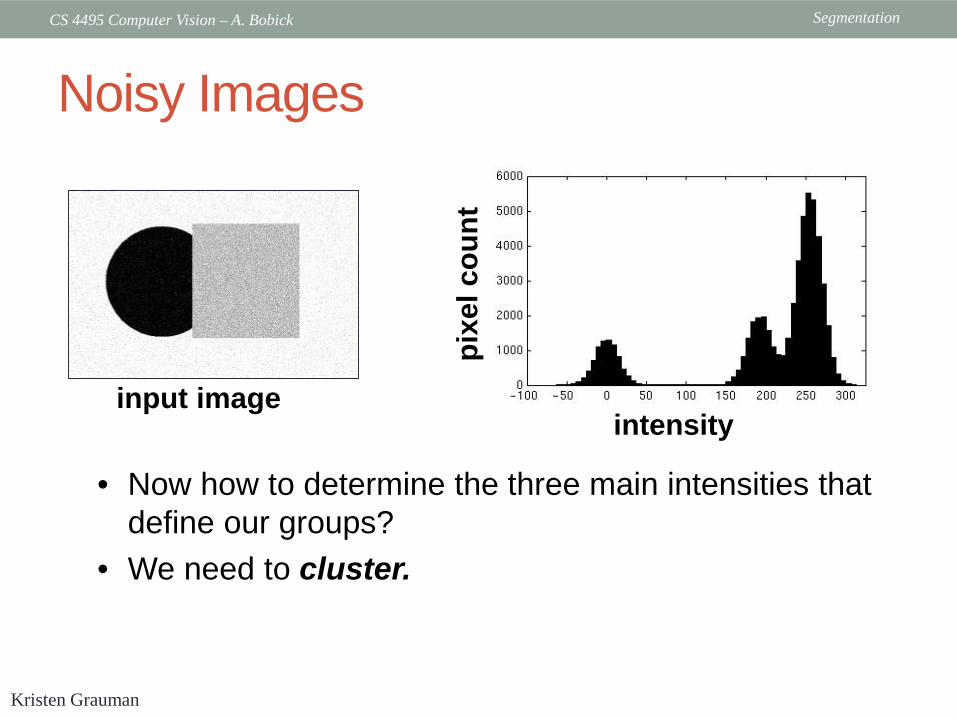
Noisy Images
SegmentationCS 4495 Computer Vision – A. Bobick
input imageintensity
pixe
l cou
nt• Now how to determine the three main intensities that
define our groups?• We need to cluster.
Kristen Grauman
Noisy Images
SegmentationCS 4495 Computer Vision – A. Bobick
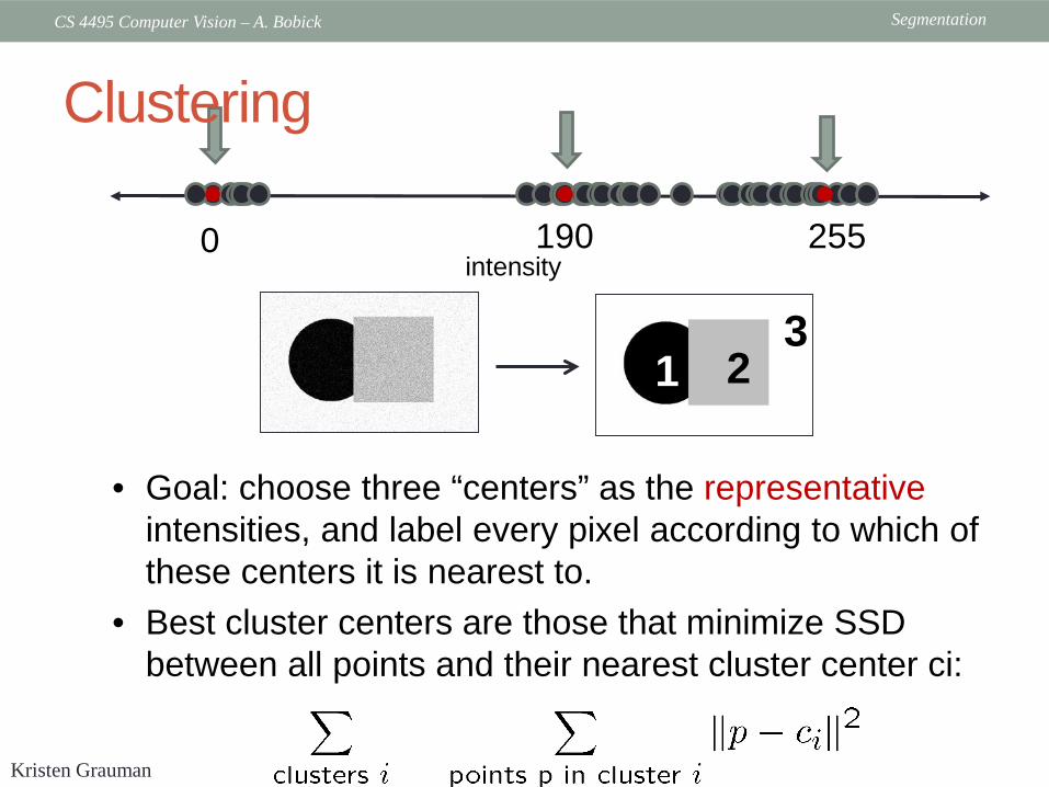
0 190 255
• Goal: choose three “centers” as the representative intensities, and label every pixel according to which of these centers it is nearest to.
• Best cluster centers are those that minimize SSD between all points and their nearest cluster center ci:
1 23
intensity
Kristen Grauman
Clustering
SegmentationCS 4495 Computer Vision – A. Bobick
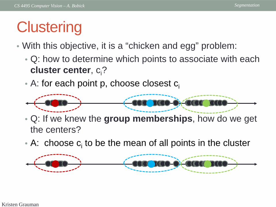
• With this objective, it is a “chicken and egg” problem:• Q: how to determine which points to associate with each
cluster center, ci?• A: for each point p, choose closest ci
• Q: If we knew the group memberships, how do we get the centers?
• A: choose ci to be the mean of all points in the cluster
Kristen Grauman
Clustering
SegmentationCS 4495 Computer Vision – A. Bobick
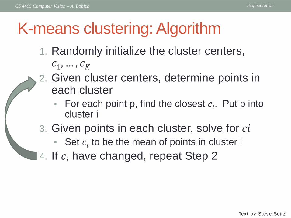
K-means clustering: Algorithm1. Randomly initialize the cluster centers, 𝑐𝑐1, … , 𝑐𝑐𝐾𝐾
2. Given cluster centers, determine points in each cluster• For each point p, find the closest 𝑐𝑐𝑖𝑖. Put p into
cluster i3. Given points in each cluster, solve for 𝑐𝑐𝑖𝑖
• Set 𝑐𝑐𝑖𝑖 to be the mean of points in cluster i4. If 𝑐𝑐𝑖𝑖 have changed, repeat Step 2
Text by Steve Seitz

SegmentationCS 4495 Computer Vision – A. Bobick
Andrew Moore

SegmentationCS 4495 Computer Vision – A. Bobick
Andrew Moore
SegmentationCS 4495 Computer Vision – A. Bobick
Andrew Moore

SegmentationCS 4495 Computer Vision – A. Bobick
Andrew Moore

SegmentationCS 4495 Computer Vision – A. Bobick
Andrew Moore
SegmentationCS 4495 Computer Vision – A. Bobick
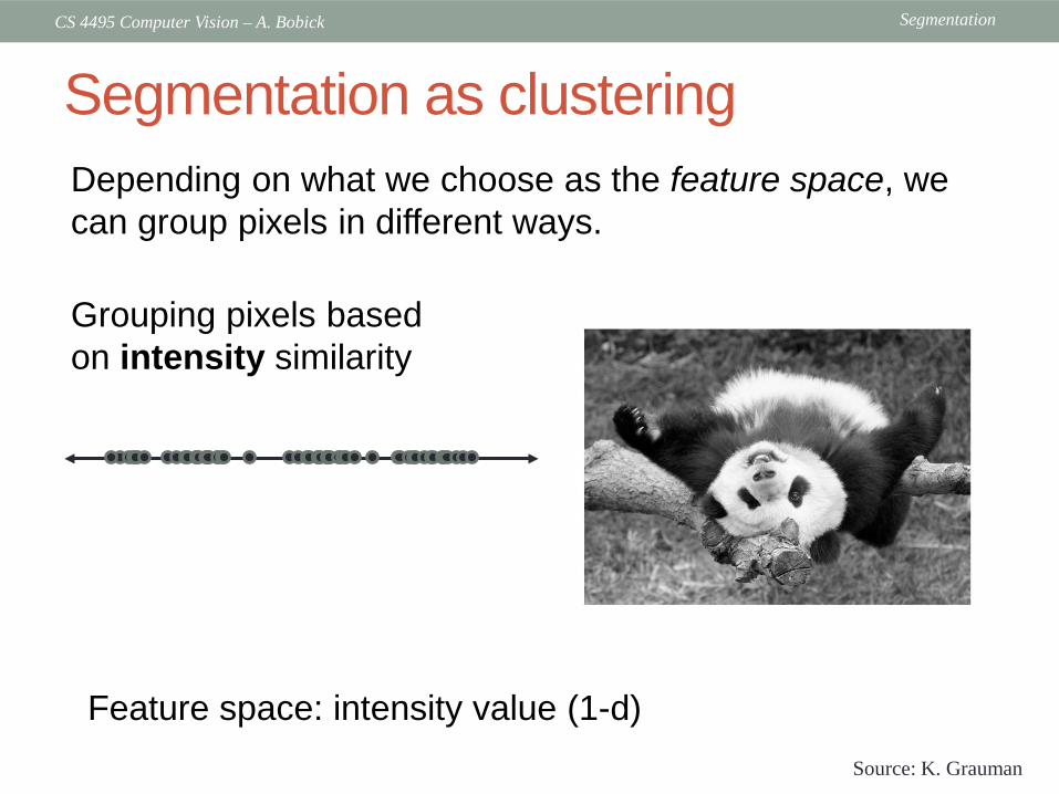
Segmentation as clusteringDepending on what we choose as the feature space, we can group pixels in different ways.
Grouping pixels based on intensity similarity
Feature space: intensity value (1-d) Source: K. Grauman
SegmentationCS 4495 Computer Vision – A. Bobick
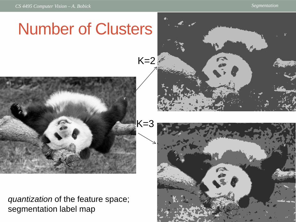
K=2
K=3
quantization of the feature space; segmentation label map
Number of Clusters

SegmentationCS 4495 Computer Vision – A. Bobick
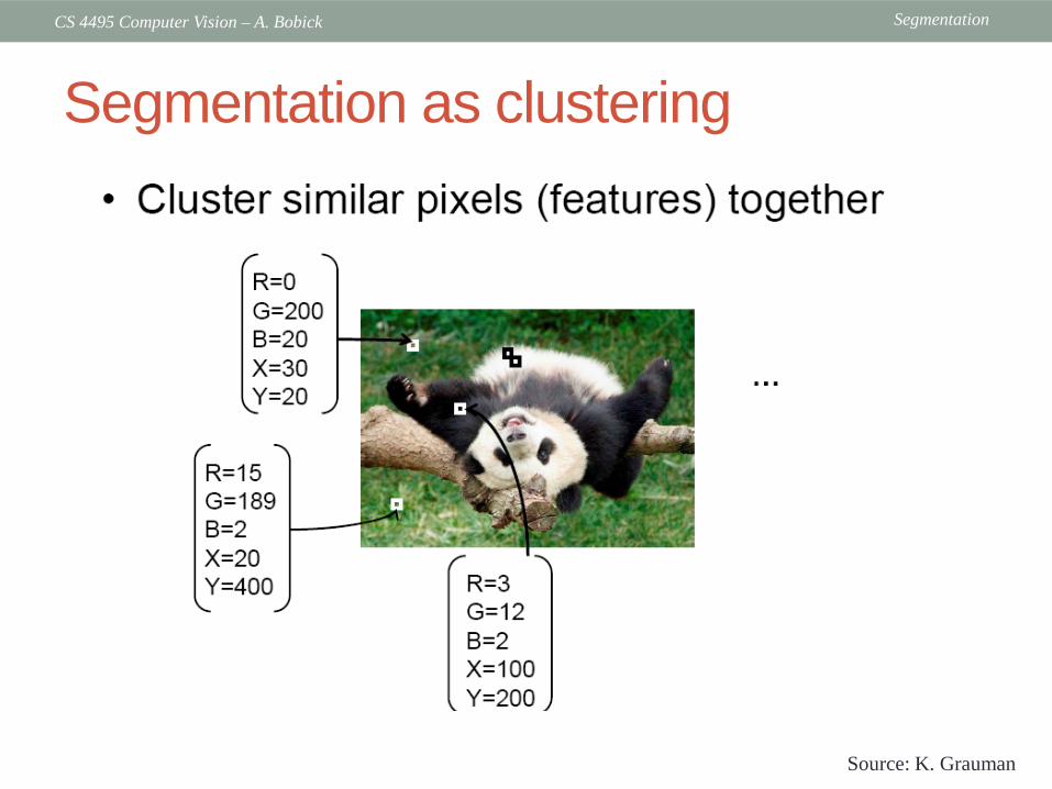
Segmentation as clustering
Depending on what we choose as the feature space, we can group pixels in different ways.
R=255G=200B=250
R=245G=220B=248
R=15G=189B=2
R=3G=12B=2R
GB
Grouping pixels based on color similarity
Feature space: color value (3-d) Kristen Grauman

SegmentationCS 4495 Computer Vision – A. Bobick
Image Intensity-based clusters Color-based clusters
Segmentation as clustering• K-means clustering based on intensity or color is
essentially vector quantization of the image attributes
Slide by Svetlana Lazebnik
SegmentationCS 4495 Computer Vision – A. Bobick
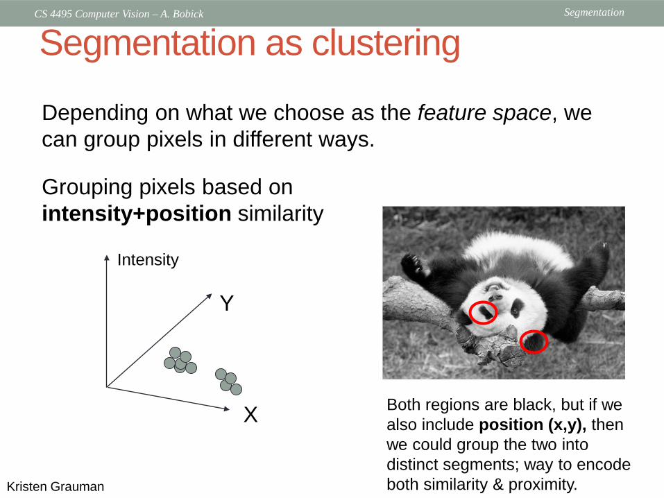
Segmentation as clustering
Depending on what we choose as the feature space, we can group pixels in different ways.
X
Grouping pixels based on intensity+position similarity
Y
Intensity
Both regions are black, but if we also include position (x,y), then we could group the two into distinct segments; way to encode both similarity & proximity.Kristen Grauman
SegmentationCS 4495 Computer Vision – A. Bobick
Segmentation as clustering
Source: K. Grauman

SegmentationCS 4495 Computer Vision – A. Bobick
Segmentation as clustering• Clustering based on (r,g,b,x,y) values enforces more
spatial coherence
Slide by Svetlana Lazebnik
SegmentationCS 4495 Computer Vision – A. Bobick
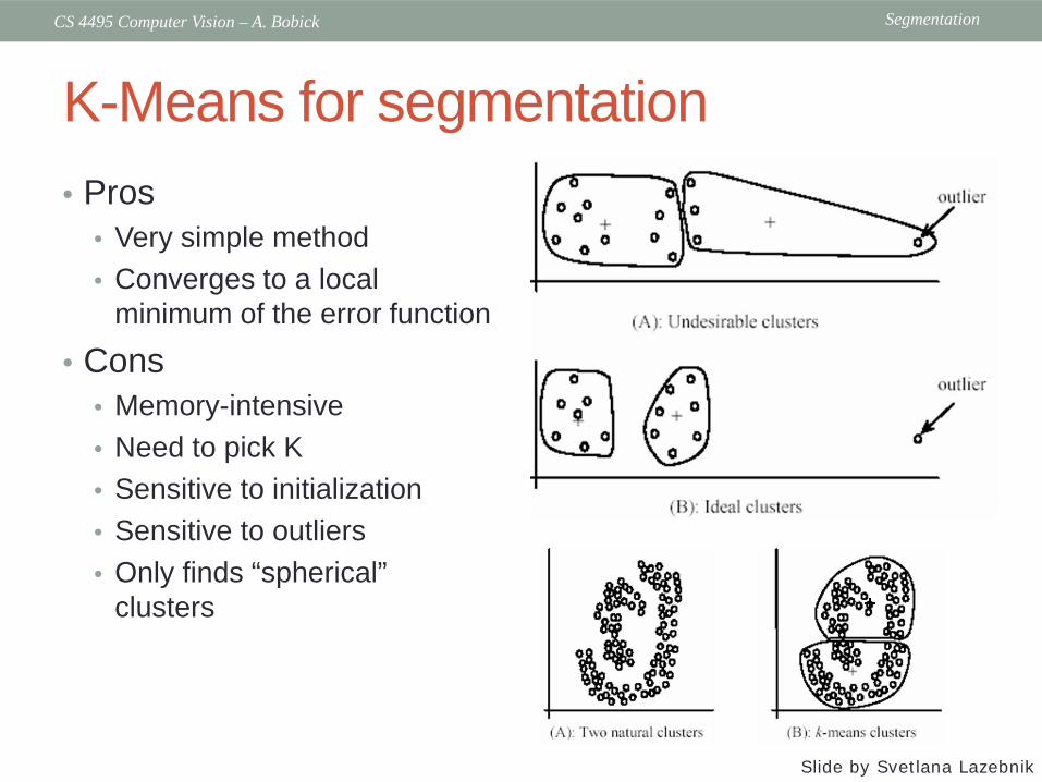
K-Means for segmentation• Pros
• Very simple method• Converges to a local
minimum of the error function
• Cons• Memory-intensive• Need to pick K• Sensitive to initialization• Sensitive to outliers• Only finds “spherical”
clusters
Slide by Svetlana Lazebnik
SegmentationCS 4495 Computer Vision – A. Bobick
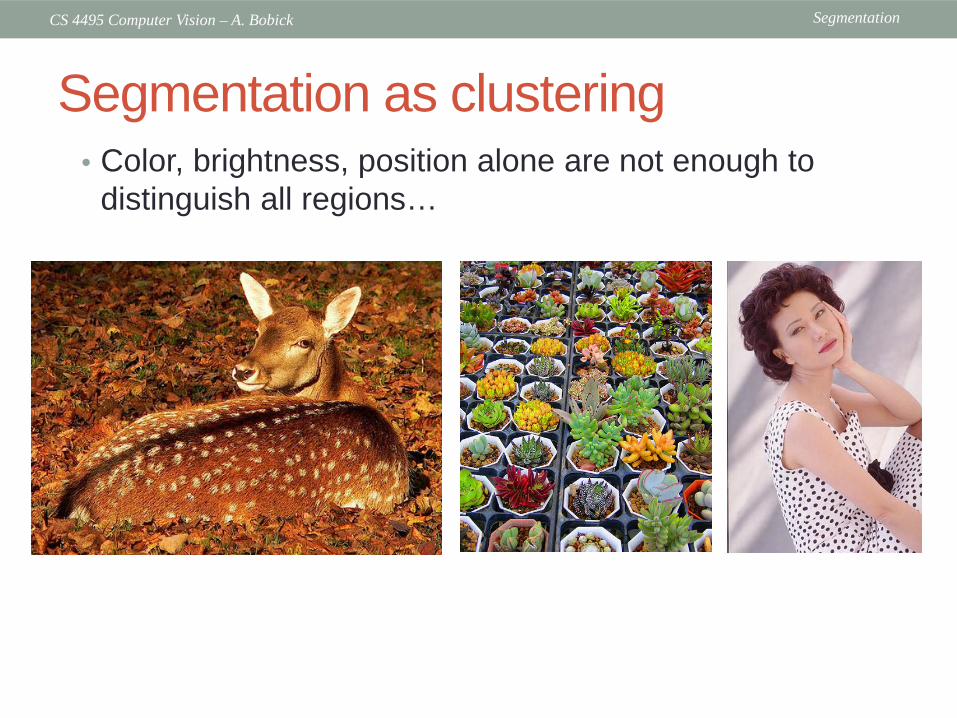
Segmentation as clustering• Color, brightness, position alone are not enough to
distinguish all regions…
SegmentationCS 4495 Computer Vision – A. Bobick
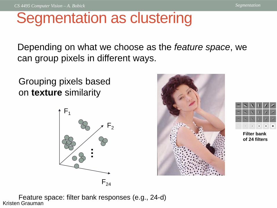
Segmentation as clustering
Depending on what we choose as the feature space, we can group pixels in different ways.
F24
Grouping pixels based on texture similarity
F2
Feature space: filter bank responses (e.g., 24-d)
F1
…
Filter bank of 24 filters
Kristen Grauman
SegmentationCS 4495 Computer Vision – A. Bobick
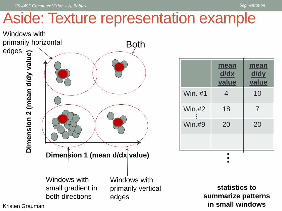
Aside: Texture representation example
statistics to summarize patterns
in small windows
mean d/dxvalue
mean d/dyvalue
Win. #1 4 10
Win.#2 18 7
Win.#9 20 20
…
…
Dimension 1 (mean d/dx value)Dim
ensi
on 2
(mea
n d/
dyva
lue)
Windows with small gradient in both directions
Windows with primarily vertical edges
Windows with primarily horizontal edges
Both
Kristen Grauman
SegmentationCS 4495 Computer Vision – A. Bobick
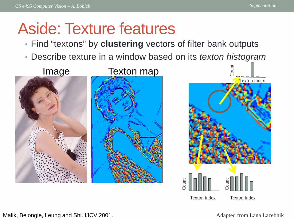
Aside: Texture features• Find “textons” by clustering vectors of filter bank outputs• Describe texture in a window based on its texton histogram
Malik, Belongie, Leung and Shi. IJCV 2001.
Texton mapImage
Adapted from Lana Lazebnik
Texton index Texton index
Cou
nt
Cou
ntC
ount
Texton index

SegmentationCS 4495 Computer Vision – A. Bobick
Image segmentation example
Kristen Grauman
SegmentationCS 4495 Computer Vision – A. Bobick
Make it better• K-means heavily sensitive to initial conditions and
(typically) need to know K in advance.
• Suppose we assume that there are a few modes in the image and that all the pixels come from these modes.
• If you could find the modes you might be able to segment the image.
SegmentationCS 4495 Computer Vision – A. Bobick
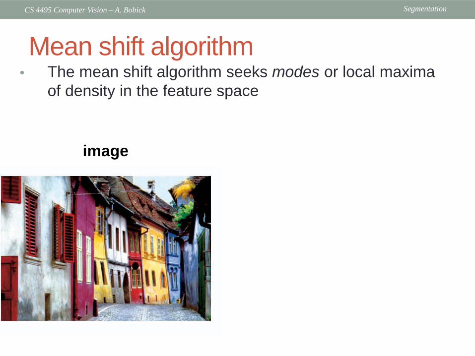
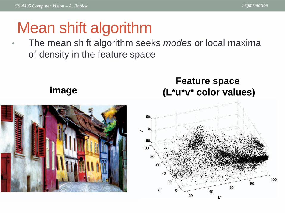
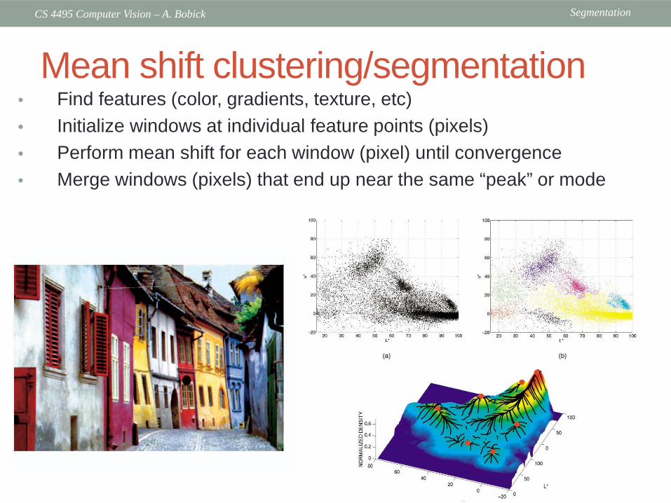
• The mean shift algorithm seeks modes or local maxima of density in the feature space
Mean shift algorithm
imageFeature space
(L*u*v* color values)

SegmentationCS 4495 Computer Vision – A. Bobick
A digression about color…• “Color” is an inherently perceptual phenomena.
• Only related but not the same as wavelength of light energy.
• In fact only some colors are found in the spectrum…
SegmentationCS 4495 Computer Vision – A. Bobick
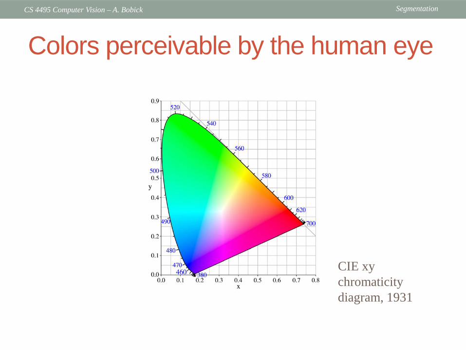
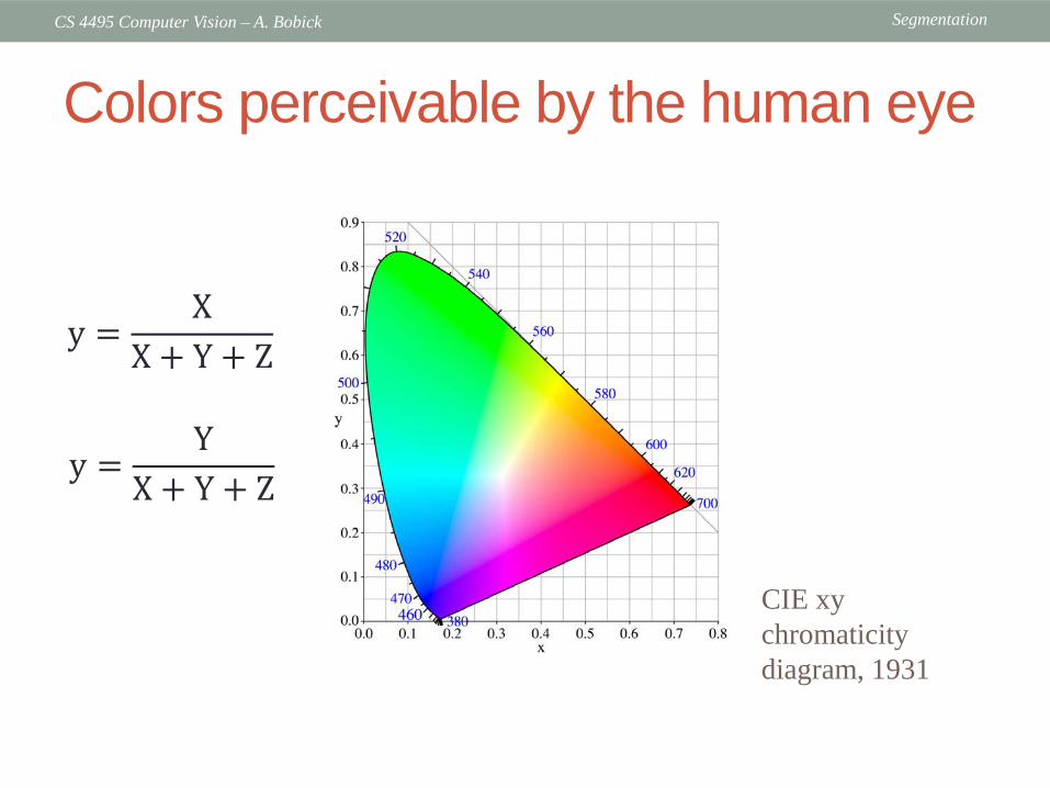
Colors perceivable by the human eye
CIE xychromaticity diagram, 1931
SegmentationCS 4495 Computer Vision – A. Bobick
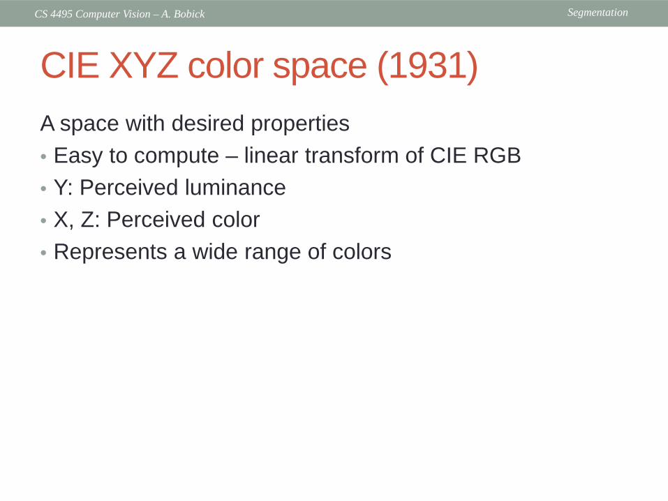
CIE XYZ color space (1931)A space with desired properties• Easy to compute – linear transform of CIE RGB• Y: Perceived luminance• X, Z: Perceived color• Represents a wide range of colors
SegmentationCS 4495 Computer Vision – A. Bobick
Colors perceivable by the human eye
CIE xychromaticity diagram, 1931
y =X
X + Y + Z
y =Y
X + Y + Z
SegmentationCS 4495 Computer Vision – A. Bobick
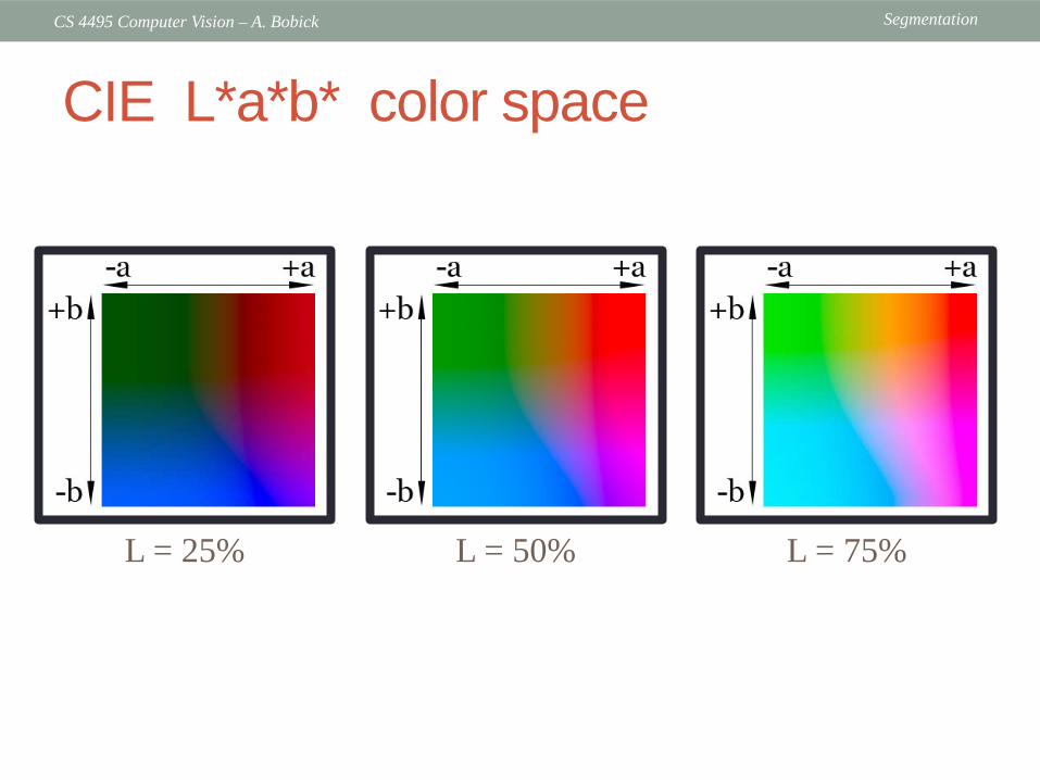
CIE L*a*b* color space
L = 25% L = 50% L = 75%

SegmentationCS 4495 Computer Vision – A. Bobick
Cylindrical view
Think of chroma(here a*, b*) defining a planar disc at each luminance level (L)

SegmentationCS 4495 Computer Vision – A. Bobick
HSL and HSV color spaces
SegmentationCS 4495 Computer Vision – A. Bobick
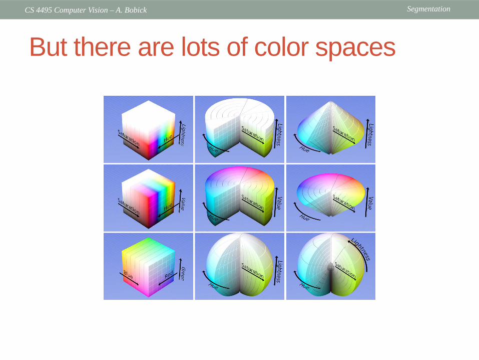
But there are lots of color spaces
SegmentationCS 4495 Computer Vision – A. Bobick
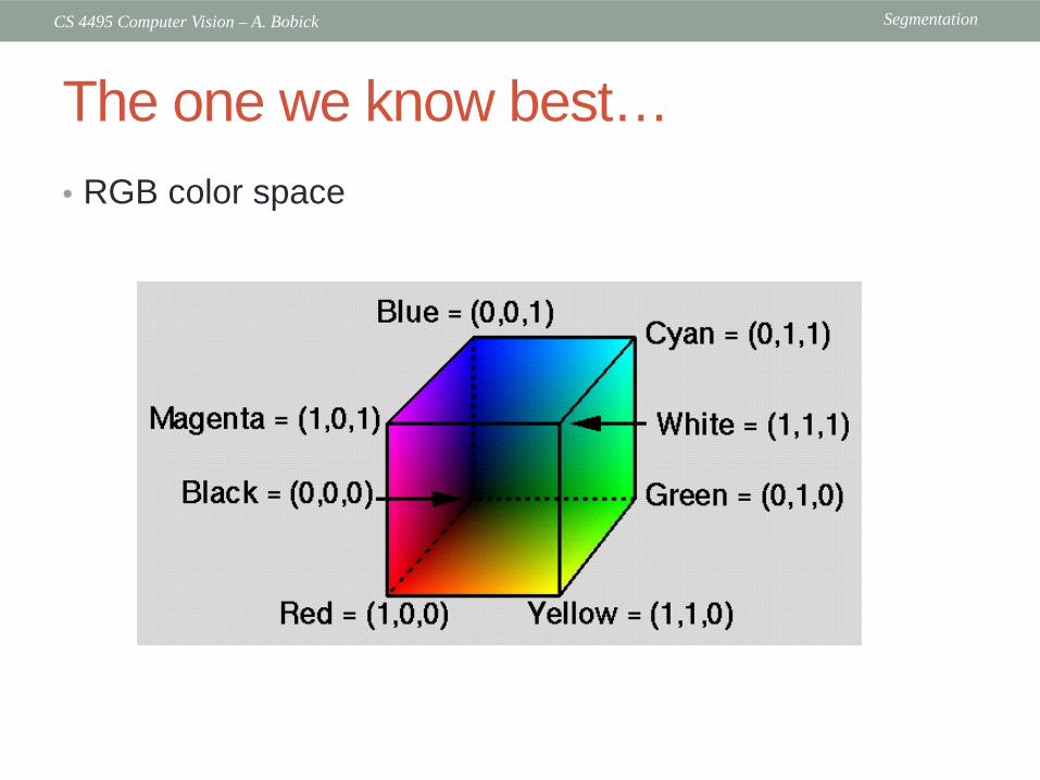
The one we know best…• RGB color space
SegmentationCS 4495 Computer Vision – A. Bobick
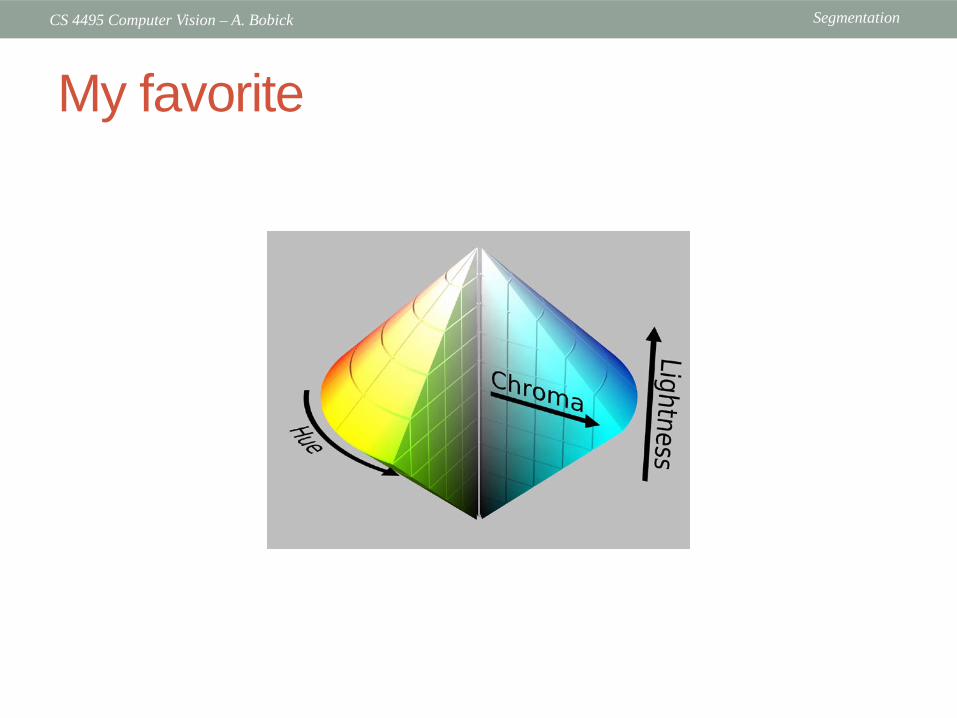
My favorite
SegmentationCS 4495 Computer Vision – A. Bobick
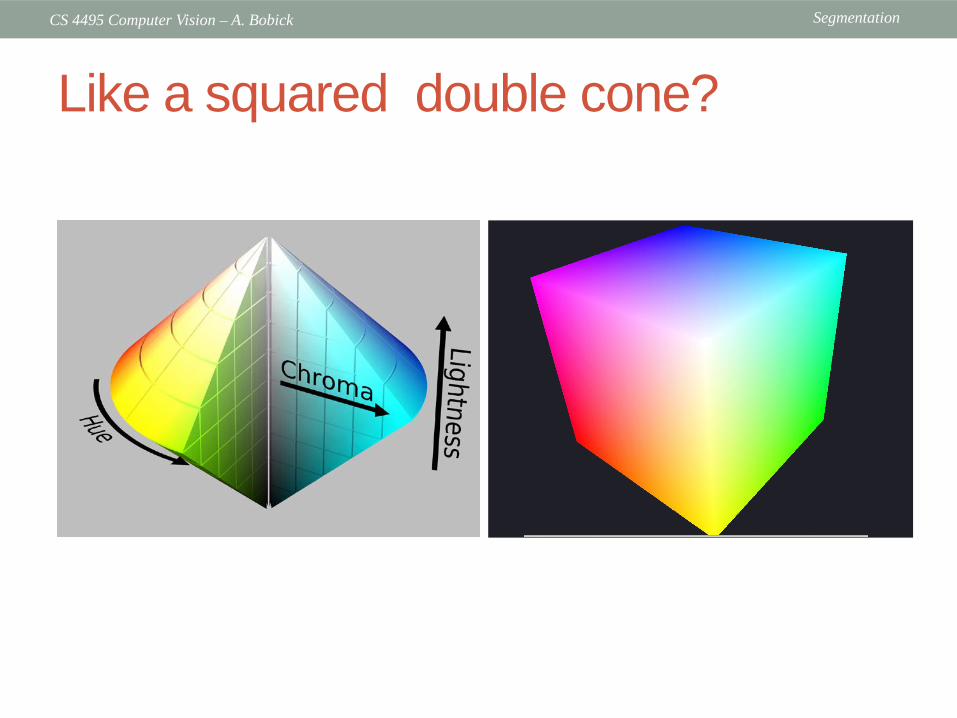
Like a squared double cone?
SegmentationCS 4495 Computer Vision – A. Bobick
• The mean shift algorithm seeks modes or local maxima of density in the feature space
Mean shift algorithm
imageFeature space
(L*u*v* color values)

SegmentationCS 4495 Computer Vision – A. Bobick
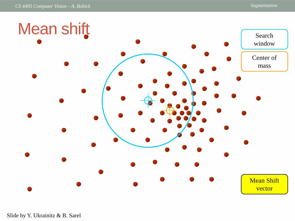
Searchwindow
Center ofmass
Mean Shiftvector
Mean shift
Slide by Y. Ukrainitz & B. Sarel

SegmentationCS 4495 Computer Vision – A. Bobick
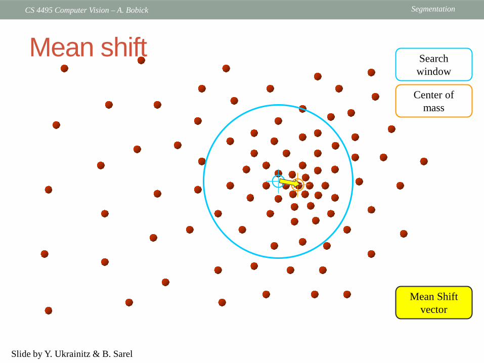
Searchwindow
Center ofmass
Mean Shiftvector
Mean shift
Slide by Y. Ukrainitz & B. Sarel

SegmentationCS 4495 Computer Vision – A. Bobick
Searchwindow
Center ofmass
Mean Shiftvector
Mean shift
Slide by Y. Ukrainitz & B. Sarel
SegmentationCS 4495 Computer Vision – A. Bobick
Searchwindow
Center ofmass
Mean Shiftvector
Mean shift
Slide by Y. Ukrainitz & B. Sarel
SegmentationCS 4495 Computer Vision – A. Bobick
Searchwindow
Center ofmass
Mean Shiftvector
Mean shift
Slide by Y. Ukrainitz & B. Sarel

SegmentationCS 4495 Computer Vision – A. Bobick
Searchwindow
Center ofmass
Mean Shiftvector
Mean shift
Slide by Y. Ukrainitz & B. Sarel
SegmentationCS 4495 Computer Vision – A. Bobick
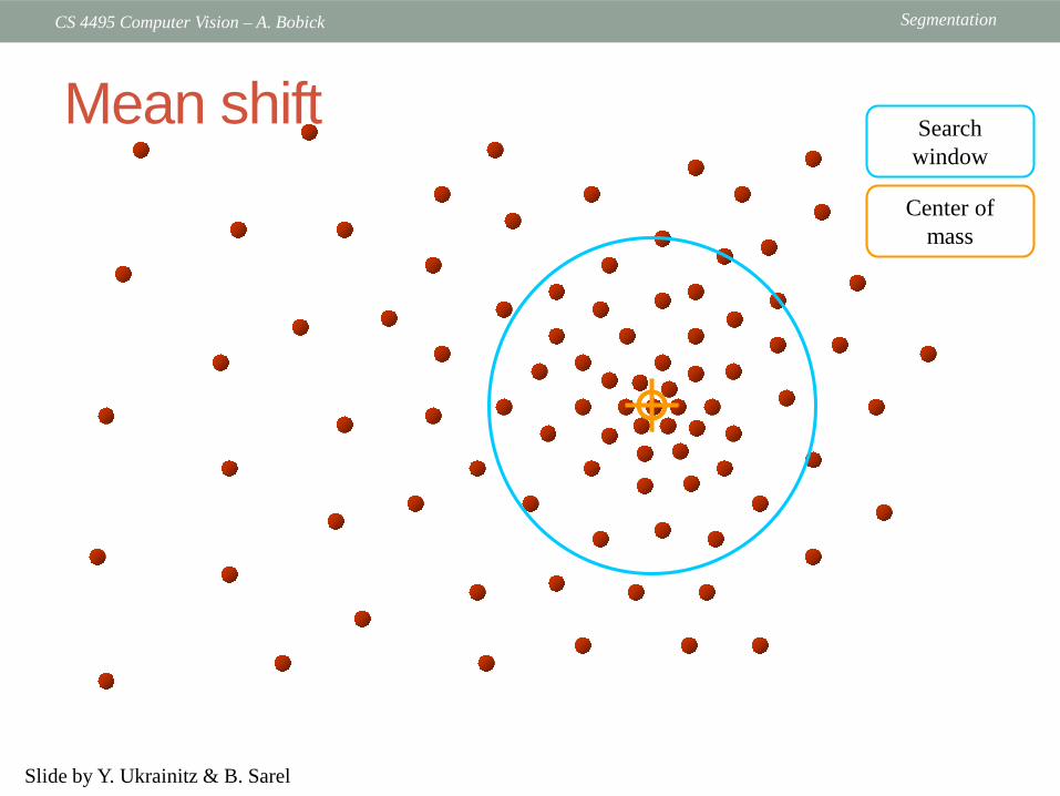
Searchwindow
Center ofmass
Mean shift
Slide by Y. Ukrainitz & B. Sarel
SegmentationCS 4495 Computer Vision – A. Bobick
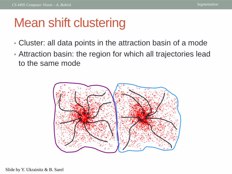
• Cluster: all data points in the attraction basin of a mode• Attraction basin: the region for which all trajectories lead
to the same mode
Mean shift clustering
Slide by Y. Ukrainitz & B. Sarel
SegmentationCS 4495 Computer Vision – A. Bobick
• Find features (color, gradients, texture, etc)• Initialize windows at individual feature points (pixels)• Perform mean shift for each window (pixel) until convergence• Merge windows (pixels) that end up near the same “peak” or mode
Mean shift clustering/segmentation
SegmentationCS 4495 Computer Vision – A. Bobick
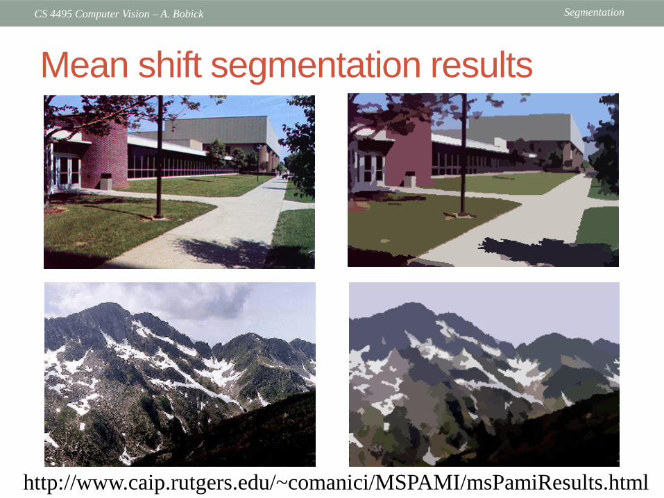
http://www.caip.rutgers.edu/~comanici/MSPAMI/msPamiResults.html
Mean shift segmentation results
SegmentationCS 4495 Computer Vision – A. Bobick
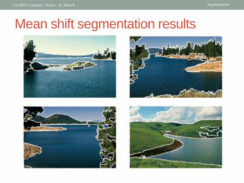
Mean shift segmentation results
SegmentationCS 4495 Computer Vision – A. Bobick
Mean shift• Pros:
• Does not assume shape on clusters• One parameter choice (window size)• Generic technique• Find multiple modes
• Cons:• Selection of window size• Does not scale well with dimension of feature space
Kristen Grauman
SegmentationCS 4495 Computer Vision – A. Bobick
q
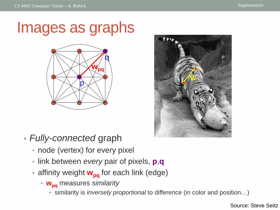
Images as graphs
• Fully-connected graph• node (vertex) for every pixel• link between every pair of pixels, p,q• affinity weight wpq for each link (edge)
• wpq measures similarity• similarity is inversely proportional to difference (in color and position…)
p
wpq
w
Source: Steve Seitz
SegmentationCS 4495 Computer Vision – A. Bobick
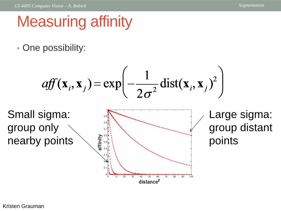
Measuring affinity• One possibility:
Small sigma: group only nearby points
Large sigma: group distant points
Kristen Grauman
SegmentationCS 4495 Computer Vision – A. Bobick
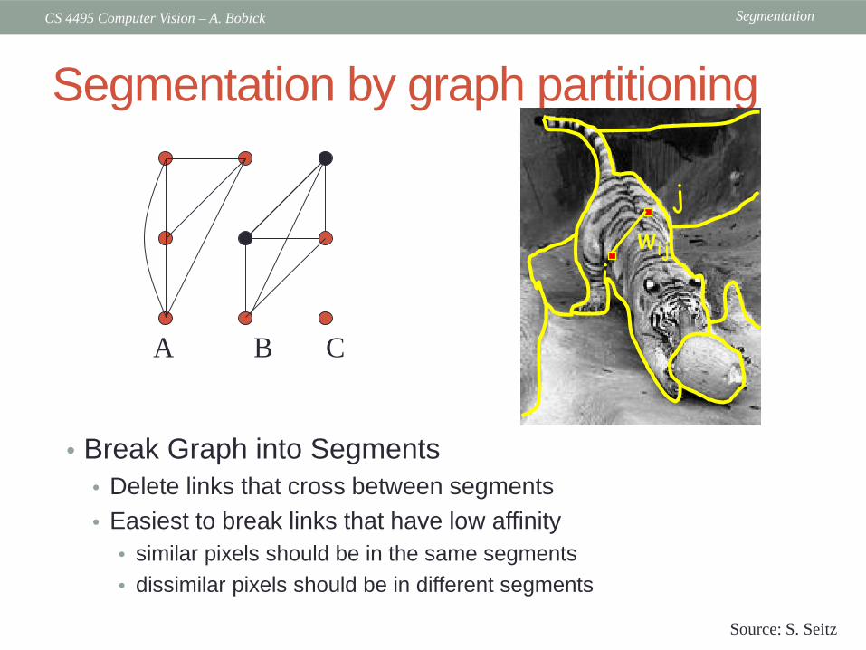
Segmentation by graph partitioning
• Break Graph into Segments• Delete links that cross between segments• Easiest to break links that have low affinity
• similar pixels should be in the same segments• dissimilar pixels should be in different segments
A B C
Source: S. Seitz
wiji
j

SegmentationCS 4495 Computer Vision – A. Bobick
Graph cut
• Set of edges whose removal makes a graph disconnected
• Cost of a cut: sum of weights of cut edges
• A graph cut gives us a segmentation• What is a “good” graph cut and how do we find one?
A B
Source: S. Seitz
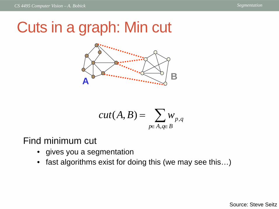
∑∈∈
=BqAp
qpwBAcut,
,),(
SegmentationCS 4495 Computer Vision – A. Bobick
Cuts in a graph: Min cut
A B
Find minimum cut• gives you a segmentation• fast algorithms exist for doing this (we may see this…)
Source: Steve Seitz
∑∈∈
=BqAp
qpwBAcut,
,),(

SegmentationCS 4495 Computer Vision – A. Bobick
Minimum cut
• Problem with minimum cut: Weight of cut proportional to number of edges in the cut; tends to produce small, isolated components.
[Shi & Malik, 2000 PAMI]
SegmentationCS 4495 Computer Vision – A. Bobick
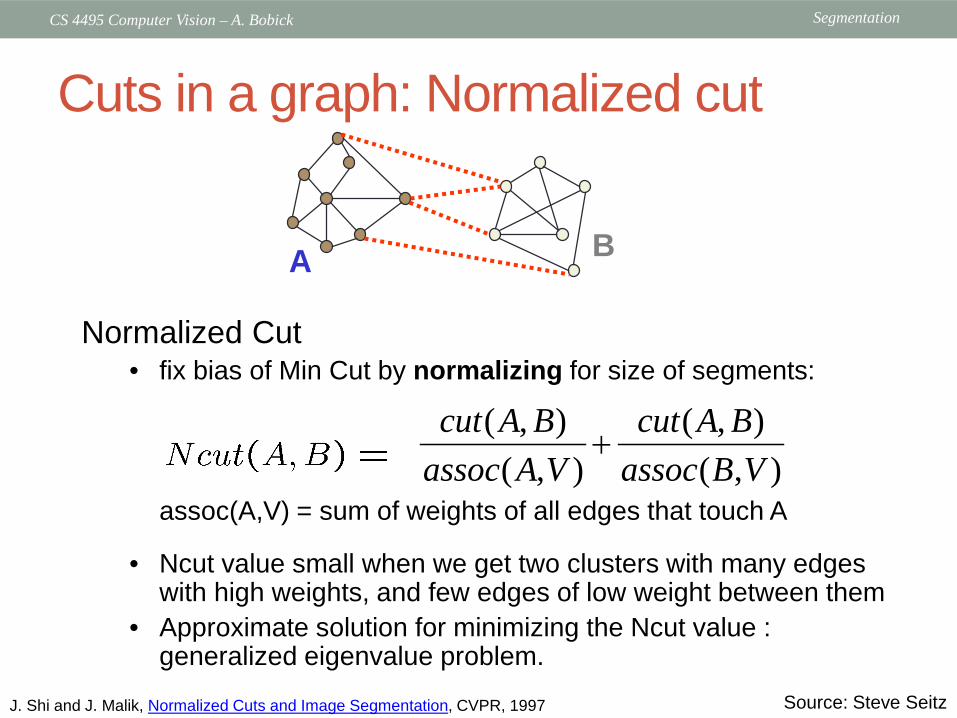
Cuts in a graph: Normalized cut
A B
Normalized Cut• fix bias of Min Cut by normalizing for size of segments:
assoc(A,V) = sum of weights of all edges that touch A
• Ncut value small when we get two clusters with many edges with high weights, and few edges of low weight between them
• Approximate solution for minimizing the Ncut value : generalized eigenvalue problem.
Source: Steve Seitz
),(),(
),(),(
VBassocBAcut
VAassocBAcut
+
J. Shi and J. Malik, Normalized Cuts and Image Segmentation, CVPR, 1997

SegmentationCS 4495 Computer Vision – A. Bobick
Example results

SegmentationCS 4495 Computer Vision – A. Bobick
Results: Berkeley Segmentation Engine
http://www.cs.berkeley.edu/~fowlkes/BSE/
SegmentationCS 4495 Computer Vision – A. Bobick
Normalized cuts: pros and cons
Pros:• Generic framework, flexible to choice of function that
computes weights (“affinities”) between nodes• Does not require model of the data distribution
Cons:• Time complexity can be high
• Dense, highly connected graphs many affinity computations• Solving eigenvalue problem
• Preference for balanced partitions
Kristen Grauman

SegmentationCS 4495 Computer Vision – A. Bobick
The end…

SegmentationCS 4495 Computer Vision – A. Bobick
Geometry of Color (CIE)
• Perceptual color spaces are non-convex
• Three primaries can span the space, but weights may be negative.
• Curved outer edge consists of single wavelength primaries
Source: Jim Rehg

SegmentationCS 4495 Computer Vision – A. Bobick
RGB Color Space
Many colors cannot berepresented(phosphor limitations)
Source: Jim Rehg
SegmentationCS 4495 Computer Vision – A. Bobick
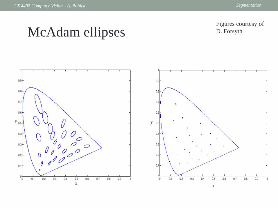
Uniform color spaces• McAdam ellipses (next slide) demonstrate that differences in x,y are a poor guide to differences in color
• Construct color spaces so that differences in coordinates are a good guide to differences in color.
Source: Jim Rehg
SegmentationCS 4495 Computer Vision – A. Bobick
Figures courtesy ofD. ForsythMcAdam ellipses

SegmentationCS 4495 Computer Vision – A. Bobick
LUV Color Space
SegmentationCS 4495 Computer Vision – A. Bobick
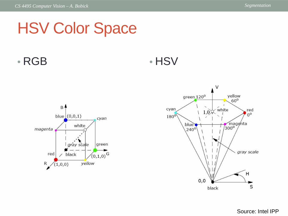
HSV Color Space
• RGB • HSV
Source: Intel IPP
SegmentationCS 4495 Computer Vision – A. Bobick
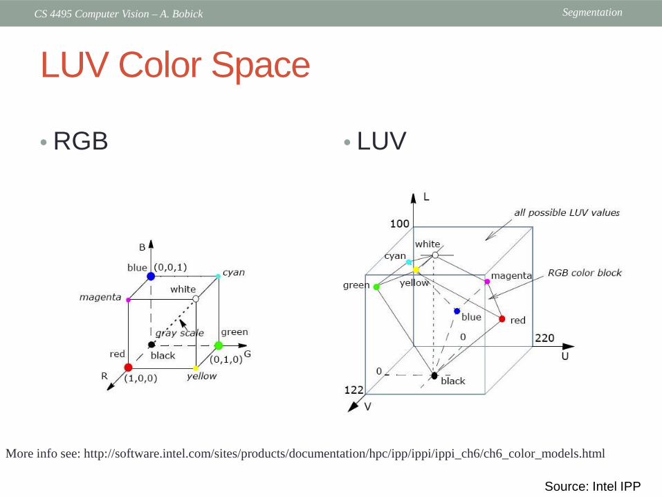
LUV Color Space
• RGB • LUV
Source: Intel IPP
More info see: http://software.intel.com/sites/products/documentation/hpc/ipp/ippi/ippi_ch6/ch6_color_models.html