Abstract - CS | Computer Science

NeuroAnimator:

Fast Neural Network Emulation and Control

of Physics-Based Models

by

Radek Grzeszczuk

A thesis submitted in conformity with the requirements

for the degree of Doctor of Philosophy

Graduate Department of Computer Science

University of Toronto

Copyright c 1998 by Radek Grzeszczuk

Abstract

NeuroAnimator:

Fast Neural Network Emulation and Control

of Physics-Based ModelsRadek Grzeszczuk

Doctor of PhilosophyGraduate Department of Computer Science

University of Toronto1998

Animation through the numerical simulation of physics-based graphics models o�ers un-surpassed realism, but it can be computationally demanding. Likewise, �nding controllersthat enable physics-based models to produce desired animations usually entails formidablecomputational cost. This paper demonstrates the possibility of replacing the numericalsimulation and control of model dynamics with a dramatically more e�cient alternative.In particular, we propose the NeuroAnimator, a novel approach to creating physically re-alistic animation that exploits neural networks. NeuroAnimators are automatically trainedo�-line to emulate physical dynamics through the observation of physics-based models inaction. Depending on the model, its neural network emulator can yield physically realisticanimation one or two orders of magnitude faster than conventional numerical simulation.Furthermore, by exploiting the network structure of the NeuroAnimator, we introduce afast algorithm for learning controllers that enables either physics-based models or theirneural network emulators to synthesize motions satisfying prescribed animation goals. Wedemonstrate NeuroAnimators for passive and active (actuated) rigid body, articulated, anddeformable physics-based models.

ii

Acknowledgements

First I would like to thank my advisor Demetri Terzopoulos and my de facto co-advisorGeo�rey Hinton. This thesis would not have been possible without their support.

I am most grateful to Demetri for his wonderful teaching philosophy. He believes thata student achieves the best results if he or she enjoys the work. Consequently, he gives hisstudents total freedom to pursue their interests. It is not surprising that so many of thembecome great scientists.

I would also like to thank Demetri for his unbounded enthusiasm, great expertise, re-sourcefulness, and patience. I could never quite understand how he can always remain soaccessible and friendly, despite being the busiest person I know.

I am indebted to Geo�rey for playing such an important role in this thesis. It has beena great pleasure working with him. His knowledge, enthusiasm, and sense of humor areunparalleled. He is a great teacher, capable of presenting very complicated concepts withease and clarity.

My special thanks go to John Platt for generously agreeing to serve as the externalexaminer of my thesis, despite his busy schedule. Special thanks go to Professor AnastasiosVenetsanopoulos for serving as the internal examiner. Many thanks to Professors EugeneFiume and Michiel van de Panne for serving on my committee and providing valuablecomments on my thesis.

I would like to acknowledge Jessica Hodgins for enabling me to perform the experimentswith the human runner model by supplying the SD/FAST mechanical model, the modelsimulation data for network training, and the display software.

I thank Zoubin Ghahramani for valuable discussions that led to the idea of the rotationand translation invariant emulator, which was crucial to the success of this work. I amindebted to Steve Hunt for procuring the equipment that I needed to carry out our researchat Intel. Sonja Jeter assisted me with the Viewpoint models and Mike Gendimenico for setup the video editing suite and helped me to use it. I thank John Funge and Michiel van dePanne for their assistance in producing animations, Mike Revow and Drew van Camp forassistance with Xerion, and Alexander Reshetov for his valuable suggestions about buildingphysical models.

I would also like to acknowledge the wonderful people of the graphics and vision labs atthe University of Toronto, and Kathy Yen for helping me to arrange the defense.

I am most grateful to my parents for their support and encouragement, and to Kasiafor her love and patience.

iii

Contents

1 Introduction 1

1.1 Overview of the NeuroAnimator Approach . . . . . . . . . . . . . . . . . . . 2

1.2 Contributions . . . . . . . . . . . . . . . . . . . . . . . . . . . . . . . . . . . 3

1.3 Thesis Outline . . . . . . . . . . . . . . . . . . . . . . . . . . . . . . . . . . 4

2 Related Work 7

2.1 Animation Through Motion Capture . . . . . . . . . . . . . . . . . . . . . . 7

2.2 Physics-Based Modeling . . . . . . . . . . . . . . . . . . . . . . . . . . . . . 7

2.2.1 Modeling Inanimate Objects . . . . . . . . . . . . . . . . . . . . . . 8

2.2.2 Modeling Animate Objects . . . . . . . . . . . . . . . . . . . . . . . 8

2.3 Control of Physics-Based Models . . . . . . . . . . . . . . . . . . . . . . . . 8

2.3.1 Constraint-Based Control . . . . . . . . . . . . . . . . . . . . . . . . 8

2.3.2 Motion Synthesis . . . . . . . . . . . . . . . . . . . . . . . . . . . . . 9

2.4 Neural Networks . . . . . . . . . . . . . . . . . . . . . . . . . . . . . . . . . 10

2.5 Connectionist Techniques for Adaptive Control . . . . . . . . . . . . . . . . 11

2.5.1 Reinforcement Learning . . . . . . . . . . . . . . . . . . . . . . . . . 11

2.5.2 Control Learning Based on Connectionist Models . . . . . . . . . . . 13

2.6 Summary . . . . . . . . . . . . . . . . . . . . . . . . . . . . . . . . . . . . . 16

3 Arti�cial Neural Networks 18

3.1 Neurons and Neural Networks . . . . . . . . . . . . . . . . . . . . . . . . . . 18

3.2 Approximation by Learning . . . . . . . . . . . . . . . . . . . . . . . . . . . 19

3.3 Backpropagation Algorithm . . . . . . . . . . . . . . . . . . . . . . . . . . . 20

3.3.1 Weight Update Rule . . . . . . . . . . . . . . . . . . . . . . . . . . . 20

3.3.2 Input Update Rule . . . . . . . . . . . . . . . . . . . . . . . . . . . . 21

3.4 Alternative Optimization Techniques . . . . . . . . . . . . . . . . . . . . . . 22

3.4.1 On-Line Training vs. Batch Training . . . . . . . . . . . . . . . . . . 22

3.4.2 Momentum . . . . . . . . . . . . . . . . . . . . . . . . . . . . . . . . 23

3.4.3 Line Searches . . . . . . . . . . . . . . . . . . . . . . . . . . . . . . . 24

3.5 The Xerion Neural Network Simulator . . . . . . . . . . . . . . . . . . . . . 25

4 From Physics-Based Models to NeuroAnimators 26

4.1 Emulation . . . . . . . . . . . . . . . . . . . . . . . . . . . . . . . . . . . . . 26

4.2 Network Structure . . . . . . . . . . . . . . . . . . . . . . . . . . . . . . . . 27

4.2.1 Weights, Hidden Units, and Training Data . . . . . . . . . . . . . . 29

4.3 Input and Output Transformations . . . . . . . . . . . . . . . . . . . . . . . 30

4.3.1 Notation . . . . . . . . . . . . . . . . . . . . . . . . . . . . . . . . . . 32

iv

4.3.2 An Emulator That Predicts State Changes . . . . . . . . . . . . . . 32

4.3.3 Translation and Rotation Invariant Emulator . . . . . . . . . . . . . 34

4.3.4 Pre-processing and Post-processing of Training Data . . . . . . . . . 35

4.3.5 Complete Step through Transformed Emulator . . . . . . . . . . . . 37

4.4 Hierarchical Networks . . . . . . . . . . . . . . . . . . . . . . . . . . . . . . 37

4.5 Training NeuroAnimators . . . . . . . . . . . . . . . . . . . . . . . . . . . . 384.5.1 Training Data . . . . . . . . . . . . . . . . . . . . . . . . . . . . . . . 38

4.5.2 Training Data For Structured NeuroAnimator . . . . . . . . . . . . . 41

4.5.3 Network Training in Xerion . . . . . . . . . . . . . . . . . . . . . . . 43

5 NeuroAnimator Controller Synthesis 44

5.1 Motivation . . . . . . . . . . . . . . . . . . . . . . . . . . . . . . . . . . . . 44

5.2 Objective Function and Optimization . . . . . . . . . . . . . . . . . . . . . 46

5.3 Backpropagation Through Time . . . . . . . . . . . . . . . . . . . . . . . . 46

5.3.1 Momentum Term . . . . . . . . . . . . . . . . . . . . . . . . . . . . . 48

5.3.2 Control Learning in Hierarchical NeuroAnimators . . . . . . . . . . 48

5.3.3 Extending the Algorithm to Arbitrary Objectives . . . . . . . . . . . 485.4 Control Adjustment Step Through Structured NeuroAnimator . . . . . . . 49

5.5 Example . . . . . . . . . . . . . . . . . . . . . . . . . . . . . . . . . . . . . . 50

6 Results 53

6.1 Example NeuroAnimations . . . . . . . . . . . . . . . . . . . . . . . . . . . 536.1.1 Performance Benchmarks . . . . . . . . . . . . . . . . . . . . . . . . 59

6.1.2 Approximation Error . . . . . . . . . . . . . . . . . . . . . . . . . . . 59

6.1.3 Regularization of Deformable Models . . . . . . . . . . . . . . . . . . 60

6.2 Control Learning Results . . . . . . . . . . . . . . . . . . . . . . . . . . . . 61

6.3 Directed vs Undirected Search in Control Space . . . . . . . . . . . . . . . . 67

6.3.1 Gradient Descent vs Momentum . . . . . . . . . . . . . . . . . . . . 67

7 Conclusion and Future Work 70

7.1 Conclusion . . . . . . . . . . . . . . . . . . . . . . . . . . . . . . . . . . . . 70

7.2 Future Research Directions . . . . . . . . . . . . . . . . . . . . . . . . . . . 71

7.2.1 Model Reconstruction . . . . . . . . . . . . . . . . . . . . . . . . . . 717.2.2 Emulator Improvements . . . . . . . . . . . . . . . . . . . . . . . . . 71

7.2.3 Neural Controller Representation . . . . . . . . . . . . . . . . . . . . 72

7.2.4 Hierarchical Emulation and Control . . . . . . . . . . . . . . . . . . 72

7.2.5 NeuroAnimators in Arti�cial Life . . . . . . . . . . . . . . . . . . . . 72

A Forward Pass Through the Network 73

B Weight Update Rule 74

C Input Update Rule 79

D Quaternions 82

D.1 Quaternion Representation . . . . . . . . . . . . . . . . . . . . . . . . . . . 82

D.2 Quaternion Rotation . . . . . . . . . . . . . . . . . . . . . . . . . . . . . . . 83

D.2.1 Rotation Negation . . . . . . . . . . . . . . . . . . . . . . . . . . . . 83

D.2.2 Rotation Summation . . . . . . . . . . . . . . . . . . . . . . . . . . . 83

v

D.3 Rotation Interpolation . . . . . . . . . . . . . . . . . . . . . . . . . . . . . . 84D.4 Matrix Representation of Quaternion Multiplication . . . . . . . . . . . . . 84D.5 Di�erentiation of Quaternion Rotation . . . . . . . . . . . . . . . . . . . . . 84D.6 Orientation Error Metric in Quaternion Space . . . . . . . . . . . . . . . . . 85

E Description of the Models 86

E.1 Multi-Link Pendulum . . . . . . . . . . . . . . . . . . . . . . . . . . . . . . 86E.1.1 SD/FAST Script . . . . . . . . . . . . . . . . . . . . . . . . . . . . . 86E.1.2 Force Computation Function . . . . . . . . . . . . . . . . . . . . . . 86

E.2 Lunar Lander . . . . . . . . . . . . . . . . . . . . . . . . . . . . . . . . . . . 87E.2.1 SD/FAST Script . . . . . . . . . . . . . . . . . . . . . . . . . . . . . 88E.2.2 Force Computation Function . . . . . . . . . . . . . . . . . . . . . . 88

E.3 Truck . . . . . . . . . . . . . . . . . . . . . . . . . . . . . . . . . . . . . . . 89E.3.1 SD/FAST Script . . . . . . . . . . . . . . . . . . . . . . . . . . . . . 89E.3.2 Force Computation Function . . . . . . . . . . . . . . . . . . . . . . 89

E.4 Dolphin . . . . . . . . . . . . . . . . . . . . . . . . . . . . . . . . . . . . . . 92E.4.1 Spring-Mass Model . . . . . . . . . . . . . . . . . . . . . . . . . . . . 92

F Example Xerion Script 94

F.1 Training Data . . . . . . . . . . . . . . . . . . . . . . . . . . . . . . . . . . . 95

G Controller Representation 96

Bibliography 98

vi

List of Figures

1.1 Menagerie of models . . . . . . . . . . . . . . . . . . . . . . . . . . . . . . . 5

2.1 Control synthesis using reinforcement learning . . . . . . . . . . . . . . . . . 12

2.2 Identi�cation of the forward model . . . . . . . . . . . . . . . . . . . . . . . 13

2.3 Identi�cation of the inverse model . . . . . . . . . . . . . . . . . . . . . . . 14

2.4 Inverse modeling . . . . . . . . . . . . . . . . . . . . . . . . . . . . . . . . . 15

2.5 Forward emulation and control learning of the truck backer-upper . . . . . 16

3.1 Arti�cial neural networks . . . . . . . . . . . . . . . . . . . . . . . . . . . . 19

3.2 The backpropagation algorithm . . . . . . . . . . . . . . . . . . . . . . . . . 21

3.3 Input update rule . . . . . . . . . . . . . . . . . . . . . . . . . . . . . . . . . 21

3.4 Limitations of the gradient descent . . . . . . . . . . . . . . . . . . . . . . . 22

3.5 The gradient descent with momentum . . . . . . . . . . . . . . . . . . . . . 24

3.6 Line search minimizations . . . . . . . . . . . . . . . . . . . . . . . . . . . . 25

4.1 Forward dynamics emulation using the NeuroAnimator . . . . . . . . . . . . 27

4.2 Three-link physical pendulum and network emulators . . . . . . . . . . . . . 28

4.3 Over�tting and under�tting of neural networks . . . . . . . . . . . . . . . . 29

4.4 . . . . . . . . . . . . . . . . . . . . . . . . . . . . . . . . . . . . . . . . . . . 31

4.5 Emulator that predicts state changes . . . . . . . . . . . . . . . . . . . . . . 33

4.6 Rotation and translation invariant network . . . . . . . . . . . . . . . . . . 34

4.7 Pre-processing and post-processing of training data . . . . . . . . . . . . . . 37

4.8 Hierarchical emulator of the runner . . . . . . . . . . . . . . . . . . . . . . . 39

4.9 Hierarchical state representation for the dolphin model . . . . . . . . . . . . 40

4.10 Sampling of the state space . . . . . . . . . . . . . . . . . . . . . . . . . . . 41

4.11 Making training examples uncorrelated . . . . . . . . . . . . . . . . . . . . . 42

4.12 Transforming the training data . . . . . . . . . . . . . . . . . . . . . . . . . 42

5.1 Models trained to locomote using the motion synthesis approach . . . . . . 45

5.2 The backpropagation through time algorithm . . . . . . . . . . . . . . . . . 47

5.3 Emulator that predicts state changes (backpropagation) . . . . . . . . . . . 50

5.4 Rotation and translation invariant network (backpropagation) . . . . . . . . 51

5.5 Pre-processing and post-processing of training data (backpropagation) . . . 51

5.6 Backpropagation step through restructured emulator . . . . . . . . . . . . . 52

6.1 Physical model of the pendulum and the emulators . . . . . . . . . . . . . . 54

6.2 Physical model of the lunar lander and its emulator . . . . . . . . . . . . . 55

6.3 Physical model of the car and its emulator . . . . . . . . . . . . . . . . . . . 56

6.4 Physical model of the dolphin and its emulator . . . . . . . . . . . . . . . . 57

vii

6.5 Emulation of the runner . . . . . . . . . . . . . . . . . . . . . . . . . . . . . 586.6 The approximation error . . . . . . . . . . . . . . . . . . . . . . . . . . . . . 606.7 Regularization of deformable models . . . . . . . . . . . . . . . . . . . . . . 626.8 Learning to swing . . . . . . . . . . . . . . . . . . . . . . . . . . . . . . . . . 636.9 Learning to land . . . . . . . . . . . . . . . . . . . . . . . . . . . . . . . . . 646.10 Learning to park . . . . . . . . . . . . . . . . . . . . . . . . . . . . . . . . . 656.11 Learning to swim . . . . . . . . . . . . . . . . . . . . . . . . . . . . . . . . . 666.12 Directed vs. undirected optimization . . . . . . . . . . . . . . . . . . . . . . 686.13 Progress of learning for the 3-link pendulum . . . . . . . . . . . . . . . . . . 686.14 Progress of learning for the lunar lander . . . . . . . . . . . . . . . . . . . . 696.15 Progress of learning for the truck . . . . . . . . . . . . . . . . . . . . . . . . 69

B.1 Model of an arti�cial neural network . . . . . . . . . . . . . . . . . . . . . . 75

E.1 The geometrical model of the lunar lander . . . . . . . . . . . . . . . . . . . 87E.2 The geometrical model of the truck . . . . . . . . . . . . . . . . . . . . . . . 90E.3 The geometrical and the physical model of the dolphin . . . . . . . . . . . . 93

G.1 A Catmull-Rom spline. . . . . . . . . . . . . . . . . . . . . . . . . . . . . . . 97

viii

Chapter 1

Introduction

Computer graphics studies the principles of digital image synthesis (Foley et al., 1990). As a�eld it enjoys enormous popularity commensurate with the visual versatility of its medium.The computer, on the one hand, can deliver hauntingly unusual forms of visual expressionwhile, on the other hand, it can produce images so real that the only trait suggesting theirelectronic identity is that they may look too perfect.

This dissertation is concerned with computer animation, an important area of computergraphics which focuses on techniques for synthesizing digital image sequences of graphicsobjects whose forms and motions are modeled mathematically in the computer. Currently,the most popular method in commercial computer animation is keyframing|a techniquethat has been adopted from traditional animation (Lasseter, 1987). In keyframing, a humananimator interactively positions graphics objects at key instants in time. The computer theninterpolates these so-called \keyframes" to produce a continuous animation. In principle,keyframing a�ords the animator a high degree of exibility and direct control in specifyingdesired motions. In practice, however, keyframing complex graphics models usually requiresa great deal of skill and intense labor on the part of the animator, especially when the taskis to create physically realistic animation in three dimensions. Hence, graphics researchersare motivated to develop animation techniques that a�ord a higher degree of automationthan is available through keyframing.

In this thesis, we are mainly interested in the process of synthesizing realistic animationin a highly automated fashion. Physical modeling is an important approach to this end.Physics-based computer animation applies the principles of Newtonian mechanics to achievephysically realistic motions. In this paradigm, the animator speci�es the physical propertiesof the graphics model and the equations that govern its motion, and the computer synthe-sizes the animation through numerical simulation of the governing equations. Once thesimulation is initialized, the outcome depends entirely on the forces acting on the physicalmodel. Physics-based animation o�ers a high degree of realism and automation; however,the animator can exercise only indirect control over the animation, by applying appropriatecontrol forces to the evolving model. The \physics-based animation control problem" is theproblem of computing the control forces such that the dynamic model produces motionsthat satisfy the goals speci�ed by the animator.

After more than a decade of development, physics-based animation techniques are begin-ning to �nd their way into high-end commercial animation systems. However, a well-knowndrawback has retarded their broader penetration|compared to purely geometric models,physical models typically entail formidable numerical simulation costs and they are di�cult

1

Chapter 1. Introduction 2

to control. Despite dramatic increases in the processing power of computers in recent years,physics-based models are still far too expensive for general use. Physics-based models havebeen underutilized in virtual reality and computer game applications, where interactivedisplay speeds are necessary. Our goal is to help make physically realistic animation ofcomplex computer graphics models fast and practical.

This thesis proposes a new approach to creating physically realistic animation thatdi�ers radically from the conventional approach of numerically simulating the equations ofmotion of physics-based models. We replace physics-based models by fast emulators whichautomatically learn to produce similar motions by observing the models in action. Ouremulators have a neural network structure, hence we dub them NeuroAnimators. A neuralnetwork is a highly interconnected network of multi-input nonlinear processing units called\neurons" (Bishop, 1995). Neural networks provide a general mechanism for approximatingcomplex maps in high dimensional spaces, a property that we exploit in our work.

The NeuroAnimator structure furthermore enables a new solution to the control prob-lem associated with physics-based models. Since the neural network approximation to thephysical model is di�erentiable, it can be used to discover the causal e�ects that the controlforces have on the actions of the model. This knowledge is essential for the design of ane�cient control learning algorithm, but it is unfortunately not available through the nu-merical simulation alone. For that reason the solution to the control problem through thephysical simulation alone is di�cult to achieve.

1.1 Overview of the NeuroAnimator Approach

Our approach is motivated by the following considerations: Whether we are dealing withrigid (Hahn, 1988; Bara�, 1989), articulated (Hodgins et al., 1995; van de Panne and Fiume,1993), or nonrigid (Terzopoulos et al., 1987; Miller, 1988) dynamic animation models, thenumerical simulation of the associated equations of motion leads to the computation of adiscrete-time dynamical system of the form

st+�t = �[st;ut; ft]: (1.1)

These (generally nonlinear) equations express the vector st+�t of state variables of the system(values of the system's degrees of freedom and their velocities) at a time �t in the futureas a function � of the state vector st, the vector ut of control inputs, and the vector ft ofexternal forces acting on the system at time t.

Physics-based animation through the numerical simulation of a dynamical system gov-erned by (1.1) requires the evaluation of the map � at every timestep, which usually involvesa non-trivial computation. Evaluating � using explicit time integration methods incurs acomputational cost of O(N) operations, where N is proportional to the dimensionality ofthe state space. Unfortunately, for many dynamic models of interest, explicit methods areplagued by instability, necessitating numerous tiny timesteps �t per unit simulation time.Alternatively, implicit time-integration methods usually permit larger timesteps, but theycompute � by solving a system of N algebraic equations, generally incurring a cost of O(N3)operations per timestep.

We propose an intriguing question: Is it possible to replace the conventional numericalsimulator, which must repeatedly compute �, by a signi�cantly cheaper alternative? Acrucial realization is that the substitute, or emulator, need not compute the map � exactly,but merely approximate it to a degree of precision that preserves the perceived faithfulness


of the resulting animation to the simulated dynamics of the physical model.Neural networks (Bishop, 1995; Hertz, Krogh and Palmer, 1991) o�er a general mecha-

nism for approximating complex maps in higher dimensional spaces.1 Our premise is that,to a su�cient degree of accuracy and at signi�cant computational savings, trained neuralnetworks can approximate maps � not just for simple dynamical systems, but also for thoseassociated with dynamic models that are among the most complex reported in the literatureto date.

The NeuroAnimator, which uses neural networks to emulate physics-based animation,learns an approximation to the dynamic model by observing instances of state transitions,as well as control inputs and/or external forces that cause these transitions. Training aNeuroAnimator is quite unlike recording motion capture data, since the network observesisolated examples of state transitions rather than complete motion trajectories. By gener-alizing from the sparse examples presented to it, a trained NeuroAnimator can emulate anin�nite variety of continuous animations that it has never actually seen. Each emulation stepcosts only O(N2) operations, but it is possible to gain additional e�ciency relative to a nu-merical simulator by training neural networks to approximate a lengthy chain of evaluationsof (1.1). Thus, the emulator network can perform \super timesteps" �t = n�t, typicallyone or two orders of magnitude larger than �t for the competing implicit time-integrationscheme, thereby achieving outstanding e�ciency without serious loss of accuracy.

The NeuroAnimator o�ers an additional bonus which has crucial consequences for ani-mation control: Unlike the map � in the original dynamical system (1.1), its neural networkapproximation is analytically di�erentiable. Since the control problem is often de�ned asan optimization task that adjusts the control parameters so as to maximize an objectivefunction, the di�erentiable properties of the neural network emulator enable us to computethe gradient of the objective function with respect to the control parameters. In fact, thederivative of the objective function with respect to control inputs is e�ciently computableby applying the chain rule. Easy di�erentiability enables us to arrive at a remarkably fastgradient ascent optimization algorithm to compute near-optimal controllers. These con-trollers produce a series of control inputs ut to synthesize motions satisfying prescribedconstraints on the desired animation. NeuroAnimator controllers are equally applicable tocontrolling the original physics-based models.

1.2 Contributions

This dissertation o�ers a uni�ed solution to the problems of e�ciently synthesizing andcontrolling realistic animation using physics-based graphics models. Our contribution inthis thesis is twofold:

1. We introduce and successfully demonstrate the concept of replacing physics-basedmodels with neural network emulators. By observing the physics-based models inaction, the emulators capture the visually salient characteristics of their motions,which they can then synthesize at a small fraction of the cost of numerically simulatingthe original models.

2. We develop a control learning algorithm that exploits the structure of the neuralnetwork emulator to quickly learn controllers through a gradient descent optimization

1Note that � in (1.1) is in general a high-dimensional map from <s+u+f 7! <s, where s, u, and f denotethe dimensions of the state, control, and external force vectors.


process. These controllers enable either the emulators or the original physics-basedmodels to produce motions consistent with prescribed animation goals at dramaticallylower costs than competing control synthesis algorithms.

3. To minimize the approximation error of the emulation, we construct a structuredNeuroAnimator that has the intrinsic knowledge about the underlying model buildinto it. The main subnetwork of the structured NeuroAnimator predicts the statechanges of the model in its local coordinate system. A cascade of smaller subnetworksforms an interface between the main subnetwork and the inputs and outputs of theNeuroAnimator. To limit the approximation error that accumulates during the emu-lation of the deformable models, we introduce the regularization step that minimizesthe deformation energy.

4. For complex dynamical systems with large state spaces we introduced hierarchicalemulators that can be trained much more e�ciently. The networks in the bottom levelof this two level hierarchy are responsible for the emulation of di�erent subsystems ofthe model, while the network at the top level of the hierarchy combines the resultsobtained by the lower level.

We have developed software for specifying and training emulators which makes useof the Xerion neural network simulator developed by van Camp, Plate and Hinton atthe University of Toronto. Using our software, we demonstrate that the neural networkemulators can be trained for a variety of some of state-of-the-art physics based models incomputer graphics. Fig. 1.1 shows the models used in our research. The emulators obtainspeed-ups of often as much as two orders of magnitude when compared against their physicalcounterparts, and yet they can emulate the models with little visible degradation to thequality of motion. We also present the solutions to a variety of non-trivial control problemssynthesized through an e�cient connectionist control learning algorithm that uses gradientinformation to drastically accelerate convergence.

1.3 Thesis Outline

Chapter 2 presents prior work in computer graphics and neural networks relevant to ourresearch. It starts the survey with the work done in computer graphics on physics-basedmodeling, and proceeds to overview the neural network research upon which we draw.

Chapter 3 de�nes a common type of arti�cial neural network and discusses techniques fortraining it, most importantly the backpropagation algorithm|a fundamental optimizationmethod used for neural network training as well as controller synthesis. The chapter includesextensions of this technique, and describes other optimization scenarios in relation to ourwork.

Chapter 4 explains the practical application of neural network concepts to the con-struction and training of di�erent classes of NeuroAnimators. It introduces a strategy forbuilding networks that avoid serious over�tting, yet are exible enough to approximatehighly nonlinear mappings. It also includes the discussion on the network input/outputstructure, the use of hierarchical networks to tackle physics-based models with large statespaces, and methods for changing the network structure to minimize the approximationerror. The chapter additionally describes a strategy for generating independent trainingexamples that ensure good generalization properties of the network, and lists the di�erentoptimization techniques used for neural network training.


Figure 1.1: A diverse set of physical models used in our research. The collection includessome of the most complex models utilized in computer graphics research to date. The topleft image shows the model of a lunar lander that was implemented as a rigid body actedupon by four independent thruster jets. The top right image shows the model of a sportutility vehicle implemented as a rigid body with constraint friction forces acting on it dueto the contact with the ground. The middle left image shows the model of a multi-linkpendulum under the in uence of gravity. The pendulum has an independent actuator ateach of its 3 joints. The middle right image shows the deformable model of a dolphinthat can locomote by generating water friction forces along its body using six independentactuators. Finally, the bottom of the �gure shows the model of a runner developed byHodgins (Hodgins et al., 1995) that we used to synthesize a running motion.


In Chapter 5 we turn to the problem of control; i.e., producing physically realistic anima-tion that satis�es goals speci�ed by the animator. We �rst describe the objective functionand its discrete approximation and then propose an e�cient gradient based optimizationprocedure that computes derivatives of the objective function with respect to the controlinputs through the back-propagation algorithm.

Chapter 6 presents a list of trained NeuroAnimators and supplies performance bench-marks and an error analysis for them. Additionally, the chapter discusses the use of theregularization step during the emulation of nonrigid models and its impact on the ap-proximation error. The second part of the chapter describes the results of applying thenew control learning algorithm to the trained NeuroAnimators. The report includes thecomparison of the new technique with the control learning techniques used previously incomputer graphics literature.

Chapter 7 concludes the thesis and presents future work.Appendix A implements a C++ functions for calculating the outputs of a neural network

from the inputs.Appendix B derives the on-line weight update rule for a simple feedforward neural

network with one hidden layer and includes a C++ implementation of the algorithm.Appendix C derives the on-line input update rule for a simple feedforward neural network

with one hidden layer and includes a C++ implementation of the algorithm.Appendix D reviews the quaternion representation of rotation, and describes the quater-

nion interpolation. For the purposes of the control learning algorithm, the appendix alsoderives the di�erentiation of the quaternion rotation and de�nes the error metric for rota-tions de�ned as quaternions.

Appendix E describes the physical models used as the emulator prototypes. For the rigidbodies we include the SD/FAST script used to build the model and the force computationfunction used by the physical simulator.

Appendix F includes an example script that speci�es and trains a NeuroAnimator, andit also speci�es the format of the training data.

Appendix G describes the controller representation used in this thesis.

Chapter 2

Related Work

In this chapter, we present prior work in the �elds of computer graphics and neural networksrelevant to our research. We survey work done in computer graphics on physics-basedmodeling and proceed to overview the neural network research upon which we draw.

2.1 Animation Through Motion Capture

Motion capture o�ers an approach to physically realistic character animation that bypassesmany di�culties associated with motion synthesis through numerical simulation. Thismethod captures motion data on a computer using sensors attached to di�erent body partsof an animal. As the animal moves, each sensor outputs to the computer a motion trackthat records changes over time in the sensor location. Once captured, the motion trackscan be applied to a computer model of the animal producing physically realistic motionwithout numerical simulation. This process can be performed very e�ciently and produceshighly realistic animations. The main limitation of motion capture is its static character.The motion data captured this way is hard to alter and cannot be concatenated easily.Computer animation research seeks to address these drawbacks (Bruderlin and Williams,1995; Unuma, Anjyo and Takeuchi, 1995; Witkin and Popovi�c, 1995; Guenter et al., 1996).

Related to our work is the idea of synthetic motion capture that collects motion data fromsynthetic models into a repertoire of kinematic actions that can be played back at interactivespeeds (Lamouret and van de Panne, 1996; Yu, 1998). This approach is particularly usefulwhen the original motion is costly to compute, as is the case for complex physics-basedmodels. Lamouret additionally discusses the possibility of creating new animations from aset of representative example motions obtained using synthetic motion capture.

Our approach also uses synthetic models as the source of data, however, it is funda-mentally di�erent. We do not build up a database of kinematic motion sequences to beused for playback. Instead, we train a neural network emulator using examples of the statetransitions to behave exactly like the physical model. Once trained, the neural network canprecisely emulate the forward dynamics of the synthetic model.

2.2 Physics-Based Modeling

We seek to develop e�cient techniques for producing physically realistic animations throughthe emulation of physics-based models. Physics-based animation involves constructing mod-els of objects and computing their motion via physical simulation. A high degree of realism

7

Chapter 2. Related Work 8

results because object motion is governed by physical laws. Additionally, since the modelsreact to the environment in a physically plausible way, the animator does not need to spendtime specifying the tedious, low-level details of the motion.

2.2.1 Modeling Inanimate Objects

Physics-based techniques have been used most successfully in the animation of inanimateobjects. In particular, physics-based techniques have been applied to the animation ofrigid bodies (Hahn, 1988; Bara�, 1989), articulated �gures (Hodgins et al., 1995; Wilhelms,1987), and deformable models (Terzopoulos et al., 1987; Terzopoulos and Fleischer, 1988;Desbrun and Gascuel, 1995; Carignan et al., 1992). Physics-based animation has also beenapplied to the simulation some more speci�c domains such as uids (Kass and Miller, 1990),gases (Stam and Fiume, 1993; Foster and Metaxas, 1997), chains (Barzel and Barr, 1988),and tree leaves (Wejchert and Haumann, 1991).

A de�ning factor of physics-based animation is the simulation through numerical inte-gration of equations of motion. This paradigm requires a speci�c model description thatincludes the physical properties such as mass, damping, elasticity, etc. Once the positionand velocity of the model is initialized, the motion speci�cation is completely automaticand depends entirely on the external forces acting on the model.

2.2.2 Modeling Animate Objects

There has been a substantial amount of research devoted to physics-based modeling ofanimate objects, such as humans and animals (Armstrong and Green, 1985; Wilhelms, 1987;Hodgins et al., 1995; Miller, 1988; Tu and Terzopoulos, 1994; Lee, Terzopoulos and Waters,1995). The distinguishing feature that di�erentiates inanimate models from animate modelsis the ability of the latter to generate internal control forces through the use of internalactuators.

Physical models of animals are among the most complex in computer graphics. Peopleare very sensitive to the perceptual inaccuracies in the simulation of animals, especially ofhumans. Therefore the complexity of the models needs to be high in order to achieve thedesired realism. The complexity of a physical model leads to numerous di�culties, one ofwhich is the time devoted to the physical simulation. The control of complex models withmultiple actuators is a daunting task.

2.3 Control of Physics-Based Models

The issue of control is central to physics-based animation research. The existing methodscan be divided into two groups: the constraint based approach and motion synthesis.

2.3.1 Constraint-Based Control

The constraint-based approach to control is characterized by the imposition of kinematicconstraints on the motion of objects (Platt and Barr, 1988). An example of this approachis when a user speci�es that a body needs to follow a certain path. There are two dominanttechniques for satisfying the constraints: inverse dynamics and constraint optimization.

Inverse dynamics techniques compute a set of \constraint forces" that satisfy a set ofkinematic constraints imposed by the user. This approach has been applied to control


both rigid models (Isaacs and Cohen, 1987; Barzel and Barr, 1988) and deformable models(Witkin and Welch, 1990). The resulting motions are physically correct because the bod-ies exhibit a realistic response to forces. However, this approach is computationally veryexpensive.

Constraint optimization methods formulate the control problem in terms of an objectivefunction which must be maximized over a time interval, subject to the di�erential equationsof motion of the physical model (Brotman and Netravali, 1988; Witkin and Kass, 1988;Cohen, 1992; Liu, Gortler and Cohen, 1994). The objective function often includes aterm that is inversely proportional to the control energy expenditure due to locomotion.The underlying assumption is that motions that require less energy are preferable. Thismethod results in an open-loop controller that satis�es the constraints and maximizes theobjective. This approach requires expensive numerical techniques. The need to symbolicallydi�erentiate the equations of motion renders it impractical for all but the simplest physicalmodels.

2.3.2 Motion Synthesis

The motion synthesis approach toward locomotion control is better suited for complexphysical models and appears more consistent with theories of learning in animals. Sincethis approach uses actuators to drive the dynamical model, it automatically constrains thecontrol forces to the proper range and does not violate physics. This paradigm allowssensors to be freely incorporated into the models which establishes sensorimotor couplingor closed-loop control. The models can therefore react to changes in the environment andsynthesize realistic controllers. To produce realistic results, motion synthesis requires high�delity models.

Motion synthesis limits signi�cantly the amount of control that the animator has overthe model, since it adds yet another level of indirection between the control parametersand the resulting motion. Therefore, the derivation of suitable actuator control sequencesbecomes a fundamental task in motion synthesis. Motion speci�cation complicates as thenumber of actuators grows, since getting the model to move often involves �nding the rightcoordination between di�erent actuators. For the most part suitable controllers have beensynthesized by hand but recently a signi�cant amount of research has been done to try toautomate control synthesis.

Hand-Crafted Controllers

Manual construction of controllers involves hand crafting control functions for a set ofmuscles. Although generally quite di�cult, this method works well on models based onanimals with well known muscle activations. Miller (Miller, 1988), for example, reproducedfamiliar motion patterns of snakes and worms using sinusoidal contraction of successivepairs of muscles along the body of the animal. Terzopoulos et al. (Terzopoulos and Waters,1990; Lee, Terzopoulos and Waters, 1995) used hand-crafted controllers to coordinate theactions of di�erent groups of facial muscles to produce meaningful expressions. But themost impressive set of controllers developed manually for deformable models to date wasconstructed by Tu (Tu and Terzopoulos, 1994) for her �sh model. She derived a highlyrealistic set of controllers that uses hydrodynamic forces to achieve forward locomotionover a range of speeds, to execute turns, and to alter body roll, pitch and yaw so that the�sh can move freely within its 3D virtual world.


Hand-crafted controllers have been most often designed for rigid, articulated �gures.Wilhelms (Wilhelms, 1987) developed \Virya" { one of the earliest human �gure animationsystems that incorporates both forward and inverse dynamics simulation. Raibert (Raib-ert and Hodgins, 1991) synthesized useful controllers for hoppers, kangaroos, bipeds, andquadrupeds by decomposing the problem into a set of simple manageable control tasks.Hodgins et al. (Hodgins et al., 1995) used similar techniques to animate a variety of mo-tions associated with human athletics. McKenna et al. (McKenna and Zeltzer, 1990) usedcoupled oscillators to simulate di�erent gaits of a cockroach. Brooks (Brooks, 1991) handcrafted similar controllers for his robots. Stewart and Cremer (Stewart and Cremer, 1992)created a dynamic simulation of a biped walking by de�ning a �nite-state machine thatadds and removes constraint equations. A good survey of the work reviewed here is thebook `Making Them Move' (Badler, Barsky and Zeltzer, 1991).

Manual construction of controllers is both tedious and di�cult, but one can use opti-mization techniques to derive control functions automatically.

Controller Synthesis

The approach is inspired by the \direct dynamics" technique which was described in thecontrol literature by Goh and Teo (Goh and Teo, 1988) and earlier references cited therein.Direct dynamics prescribes a generate-and-test strategy that optimizes a control objectivefunction through repeated forward dynamic simulation and motion evaluation. This ap-proach resembles trial-and-error learning process in humans and animals and is thereforeoften referred to as \learning". It di�ers from the constraint optimization approach in thatit does not treat physics as constraints and it represents motion in actuator-time space andnot state-time space.

The direct dynamics technique was developed further to control articulated muscu-loskeletal models in (Pandy, Anderson and Hull, 1992) and it has seen application in themainstream graphics literature to the control of planar articulated �gures (van de Panneand Fiume, 1993; Ngo and Marks, 1993). Pandy et al. (Pandy, Anderson and Hull, 1992)search the model actuator space for optimal controllers, but they do not perform globaloptimization. Van de Panne and Fiume (van de Panne and Fiume, 1993) use simulated an-nealing for global optimization. Their models are equipped with simple sensors that probethe environment and use the sensory information to in uence control decisions. Ngo andMarks' (Ngo and Marks, 1993) stimulus-response control algorithm presents a similar ap-proach. They apply the genetic algorithm to �nd optimal controllers. The genetic algorithmis also used in the recent work of Sims (Sims, 1994). Ridsdale (Ridsdale, 1990) reports anearly e�ort at controller synthesis for articulated �gures from training examples using neuralnetworks. Grzeszczuk and Terzopoulos (Grzeszczuk and Terzopoulos, 1995) target state-of-the-art animate models at the level of realism and complexity of the snakes and worms ofMiller (Miller, 1988) and the �sh of Tu and Terzopoulos (Tu and Terzopoulos, 1994). Theirmodels �rst acquire a set of basic motor skills, store them in memory using compact rep-resentations, and �nally reuse them to synthesize aggregate behaviors. In ((van de Panne,1996)), van de Panne automatically synthesizes motions for physically-based quadrupeds.

2.4 Neural Networks

Research in neural networks dates as far back as the 1960s, when Widrow and co-workersproposed networks they called adalines (Widrow and Lehr, 1990). The name adaline is an


acronym derived from ADAptive LINear Element, and it refers to a single processing unitwith threshold non-linearity. At approximately the same time, Rosenblatt (Rosenblatt,1962) studied similar single layer networks which he called perceptrons. He developed alearning algorithm for perceptrons and proved its convergence. This result generated muchexcitement and ignited hopes that neural networks can be used as a basis for arti�cialintelligence. Although quite successful at solving certain problems, perceptrons failed toconverge to a solution on other seemingly similar tasks. Minsky and Papert (Minsky andPapert, 1969) pointed out that the convergence theorem for single-layer networks appliesonly to classi�cation problems of sets that are linearly separable, and therefore are notcapable of universal computation.

Although researchers had realized that the limitations of the perceptron could have beenovercome by networks having more layers of units, they failed to develop a suitable weightadjustment algorithm for training such networks. In 1986, Rumelhart, Hinton and Williams(Rumelhart, Hinton and Williams, 1986) proposed an e�cient technique for training multi-layer feed-forward neural networks which they called the backpropagation algorithm. Thealgorithm de�nes an approximation error which is a di�erentiable function of the weightsof the network, and computes recursively the derivatives of the error with respect to theweights. The derivatives can be used to adjust the weights so as to minimize the error.Similar algorithms had been developed by a number of researchers including Bryson andHo (Bryson and Ho, 1969), Werbos (Werbos, 1974), and Parker (Parker, 1985).

The class of networks with two layers of weights and sigmoidal hidden units has provento be important for practical applications. It has been shown that such networks can ap-proximate arbitrarily well any multi-dimensional functional mapping. Many papers have ap-peared in the literature discussing this property including (Cybenko, 1989; Hornik, Stinch-comb and White, 1989).

Minsky and Papert (Minsky and Papert, 1969) showed that any recurrent network canbe represented as a feed-forward network by simply unfolding the units of the networkover time. Rumelhart et al. (Rumelhart, Hinton and Williams, 1986) showed the correctform of the learning rule for such a network and used it to train a simple network to bea shift register and to complete sequences. The learning algorithm is a special version ofthe backpropagation algorithm commonly referred to as backpropagation through time. Inthis work, the emulator networks form a special class of recurrent neural networks, andbackpropagation through time constitutes the backbone of the control learning algorithm.

2.5 Connectionist Techniques for Adaptive Control

Our work is closely related to research described in the mainstream neural network literatureon connectionist techniques for the adaptive control of physical robots. Barto gives a concise,yet informative, introduction to connectionist learning for adaptive control in (Barto, 1990).Motor learning is usually formulated as an optimization process in which the motor task tobe learned is �rst speci�ed in terms of an objective function and an optimization methodis then used to compute the extremum of the function.

2.5.1 Reinforcement Learning

Reinforcement learning, an approach described by Mendel and McLaren (Mendel andMcLaren,1970), addresses the problem of controlling a system. Reinforcement learning involves two


World

Critic

ReactiveAgent

situation/state action

reward

Figure 2.1: Reinforcement learning builds an approximation|the adaptive critic|thatlearns the e�ects of current actions on future events. It then uses the system performanceinformation supplied by the critic to synthesize a controller.

problems. The �rst requires the construction of a critic that evaluates the system perfor-mance according to some control objective. The second problem is how to adjust controlsbased on the information supplied by the critic. Fig. 2.1 illustrates this process.

Reinforcement learning is most often used when a model of the system is unavailable andwhen its performance can be evaluated only by sampling the control space. This means weonly have the performance signal available, but not its gradient, and we are therefore forcedto search by actively exploring di�erent control actions and incorporating those giving goodresults into the control rules. Reinforcement learning technique resembles learning by trialand error which selects behaviors according to its likelihood of producing reinforcement|hence the name \reinforcement learning".

Reinforcement learning builds an approximation|the adaptive critic|that learns thee�ects of current actions on future events (Sutton, 1984). The critic outputs the estimate ofthe total future utility which will arise from present situations and actions. Reinforcementlearning performs in essence a gradient descent on the evaluation surface that it builds fromthe discrete examples obtained during the trial-and-error search through the control space.This approach is illustrated by the pole balancing example of Barto, Sutton and Anderson(Barto, Sutton and Anderson, 1983). Related methods that combine reinforcement learningwith the gradient have also been studied (Sutton, 1984; Anderson, 1987; Barto and Jordan,1987; Williams, 1988).

Since the active critic synthesis requires many trials, it is costly. Reinforcement istherefore ine�cient, but it's very general. Werbos writes in (Werbos, 1990): \Adaptivecritic is an approximation to dynamic programming which is the only exact and e�cientmethod available to control motors or muscles over time so as to maximize the utilityfunction in a noisy, nonlinear environment, without making highly specialized assumptionsabout this environment."

The controller synthesis techniques described in Section 2.3.2 resemble reinforcementlearning in that they actively explore the control space of the system searching for optimalcontrol actions. They di�er in that they do not synthesize the active critic and are thereforeless e�cient.


Σ+

−

dynamicalsystem

systemmodel

x(t) y(t)

y (t)i

error

Figure 2.2: During training of the forward model, the input to the network x(t) is the sameas the input to the system, and the system output y(t) forms the target output for thenetwork. The neural network is trained through the use of the prediction error, y(t)�yi(t),that measures the di�erence between the target output of the network and its true output.

2.5.2 Control Learning Based on Connectionist Models

Connectionist control learning techniques often rely on an internal model in the form ofa neural network that gives the robot system knowledge about itself and its environment.For example, the system builds an internal model of its dynamics so that it can predict itsresponse to a force stimulation. Alternatively, it can build a model of its inverse dynamicsso that it can predict a control sequence that will result in a speci�c action. These internal,neural network models need not be highly accurate approximations. Even an inaccuratemodel of inverse dynamics can provide a satisfactory control sequence whose error can becorrected with a feedback controller. Similarly, an inaccurate model of forward dynamicscan be used within an internal feedback loop which corrects the controller error.

In several cases, connectionist approximations of dynamical systems have been con-structed as a means to robot control. In this approach, a neural network learns to act likethe dynamical system by observing the system's input-output behavior as shown in Fig. 2.2.The neural network is trained through the use of the prediction error: y(t)�yi(t). A neuralnetwork trained to approximate the dynamical system is referred to as the forward model.

A neural network can approximate the inverse of a dynamical system, which then canbe used for control purposes. Jordan (Jordan, 1988) calls this the direct inverse approach.Fig. 2.3 shows a simple scenario where the dynamical system receives torque inputs x(t)and outputs the resulting trajectory y(t). The inverse dynamics model is set in the oppositedirection, i.e., it receives y(t) as input and outputs x(t). Since the inverse model forms amap from desired outputs y(t) to inputs x(t) that produce those outputs, it is in essence acontroller that can be used to control the system.

This approach was proposed and used by Albus (Albus, 1975), Widrow et al. (Widrow,McCool and Medo�, 1978), Miller et al. (Miller, Glanz and Kraft, 1987), and Jordan(Jordan, 1988). The method has been used to learn inverse kinematics (Kuperstein, 1987;Grossberg and Kuperstein, 1986), and inverse dynamics (Kawato, Setoyama and Suzuki,1988). Atkeson and Reinkensmeyer (Atkeson and Reinkensmeyer, 1988) used content ad-dressable memories to model the inverse dynamics, that accomplish learning in just oneiteration by performing a table lookup. The �rst prediction application using a non-linearneural network was published in (Lapedes and Farber, 1987). See also (Weigend and Ger-shenfeld, 1994).

The direct inverse modeling technique has a number of limitations. Most importantly,


inversedynamics

model

x(t) y(t)

error

x (t)i

Σ+

−

dynamicalsystem

Figure 2.3: The inverse dynamics model is set in an opposite direction to that of thedynamical system.

the identi�cation of the inverse dynamics model is problematic when the inverse is not wellde�ned. Ill-posedness occurs when the mapping from outputs to inputs is many-to-one,in which case the network tends to average over the various targets mapping to the sameinput (Jordan, 1988). Additionally, the training of the inverse model requires extensivesampling of the control space in order to �nd an acceptable solution. However, since thecontrol learning process requires the actual system output, extensive data collection mightnot always be feasible. An additional disadvantage of this approach is its o�-line character.

An alternative class of algorithms learn the controller indirectly through the use of theforward model of the system. This approach comprises two stages|stage one learns theforward model as described above, stage two uses the forward model to learn the controller.

With a di�erentiable forward model one can solve problems of optimization over timeusing the backpropagation through time algorithm that essentially integrates the systemmodel over time to predict future outcome and then backpropagates the error derivativeback in time to compute precisely the e�ect of current actions on future results. Whenworking with large sparse systems this methods permits the computation of derivatives ofthe utility very quickly. This technique was described by Werbos (Werbos, 1974; Werbos,1988), Jordan and Rumelhart (Jordan and Rumelhart, 1992), and Widrow (Widrow, 1986;Nguyen and Widrow, 1989). Narendra and Parthasarathy (Narendra and Parthasarathy,1991) propose a quicker optimization alternative to using backpropagation through time.

This method has advantages over the direct identi�cation of the system inverse when theinverse is not well de�ned (Jordan and Rumelhart, 1992). The ill-posedness of the problemdoes not prevent it from converging to a unique solution since it uses gradient informationto adjust the control signal in order to reduce the performance error. The system headstowards one of the solutions; the direct inverse, on the other hand, does not converge to acorrect solution. An additional feature of this approach is the use of a uniform parameteradjustment mechanism (the backpropagation algorithm) during the system identi�cationstage and the control learning stage.

Control learning techniques that utilize the forward model become particularly usefulwhen the system itself is not analyzable or it is not possible to di�erentiate it, which isoften the case for complex systems.

Forward and Inverse Modeling

Jordan and Rumelhart (Jordan and Rumelhart, 1992) proposed a scheme to combine theforward model and its inverse. The �rst stage of this process learns the forward model of the


x(t)controllermodel

y(t) forwardmodel

y (t)i

error

− Σ+

Figure 2.4: The control learning phase of the inverse modeling algorithm of Jordan andRumelhart. This method backpropagates the prediction error through the forward modelto calculate the error in the motor command, which is then used as the error signal fortraining the inverse. The dashed line shows the error signal pass through the forwardmodel before reaching the inverse model during the backpropagation step.

controlled object using the technique described in Section 2.5.2. The second stage, shown inFig. 2.4, trains the inverse dynamics model. During the control learning phase, the algorithmfeeds the forward model network the desired trajectory y(t) which computes the feedforwardmotor command xi(t). The prediction error, y(t) � yi(t), is then backpropagated throughthe forward model to calculate the error in the motor command, which is then used as theerror signal for training the inverse. During the control learning phase the parameters ofthe forward model are �xed and only the parameters of the controller are adjusted. Whenthe control learning stage is �nished the controller together with the forward model forman identity transformation.

The Truck Backer-Upper

The control learning strategy presented in this thesis resembles most closely the approachused by Nguyen and Widrow in (Nguyen and Widrow, 1989) where they develop a two-stage control learning process. The �rst stage trains a neural network to be an emulator forthe truck and trailer kinematics using the technique for system identi�cation described inSection 2.5.2. The second stage trains a neural-network controller to control the emulator.Once the controller knows how to control the emulator, it is then able to control the actualtruck.

Fig. 2.5 illustrates the procedure for adapting the controller. In the �gure, the blocklabeled T represents the trailer truck emulator. The truck emulator takes as input the stateof the model at time i and the steering signal, and outputs the state of the model at timei + 1. The block labeled C represents the neural network controller that takes as inputsthe state of the model and outputs the steering signal for the truck. The �rst step of thisprocess, shown in the top half of the �gure, computes the motion trajectory of the truck fora given controller through the forward simulation. The second step of this process, shownin the bottom half of the �gure, uses the trajectory obtained in the �rst step to evaluate theerror in the objective function, and then computes the derivative of this error with respectto the controller weights using backpropagation through time.

The control learning process starts by setting the truck initial position, and choosingthe controller weights at random. The truck backs up, until it stops. The �nal error inthe truck position is used by the backpropagation algorithm to adapt the controller. Theweights are changed by the sum of error deltas computed over all iterations using steepestdescent.


CT

s1 CT

s2 CT

sMs3 sM+1

CT

s1 CT

s2 CT

sMs3 sM+1

+Σ

−

sM+1d

error

Figure 2.5: Forward emulation of the truck kinematics (top) and training of a neural-networkcontroller to control the emulator (bottom).

The synthesized controller can park the truck in the desired position from any initialcon�guration. Since the solution learned by the controller is substantially general, it israther di�cult to �nd. To arrive at the solution, the control learning algorithm needs toprocess a large set of training examples and therefore converges slowly. Additionally, sincethe training data must have examples corresponding to di�erent initial con�gurations ofthe truck, it must be generated o�-line. Finally, the main disadvantage of the proposedcontroller representation is its static character|every time the objective function changesthe controller needs to be completely relearned. This approach is therefore not suitable fordynamic environments where control objectives change over time.

Although related to Nguyen and Widrow's paper, the work presented in this thesisdi�ers signi�cantly from it: In order to achieve a better performance, the emulators havebeen trained to approximate a chain of evaluations of a numerical simulator as describedin Section 4.1. Hierarchical emulators, discussed in Section 4.4, have been introduced toapproximate highly complex, deformable models used in computer graphics.

Our technique also o�ers a di�erent controller synthesis approach that works well indynamic environments with changing control objectives. Our controllers solve the problemof getting from a given initial con�guration to a given �nal con�guration, and thereforeare much easier to synthesize than the general controllers used by Nguyen and Widrow.Since our control synthesis algorithm works on-line from a few training examples that getupdated after each iteration, it converges very rapidly.

2.6 Summary

To date, network architectures have found rather few applications in computer graphics.One application has been the control of animated characters. Ridsdale (Ridsdale, 1990)reports a method for skill acquisition using a connectionist model of skill memory. Thesensor-actuator networks of van de Panne and Fiume (van de Panne and Fiume, 1993) arerecurrent networks of units that take sensory information as input and produce actuatorcontrols as output. Sims (Sims, 1994) employs a network architecture to structure simple\brains" that control evolved creatures. Our work di�ers fundamentally from these e�orts;it is more closely related to the neural netowrk research on control.


As we have seen in this chapter, neural network researchers have devoted a signi�cantamount of attention to control. Although we draw upon their work, especially that in(Nguyen and Widrow, 1989), we must adapt existing techniques to �t the requirements ofcomputer animation. The theme of our work is to use connectionist techniques to tacklethe fundamental problems of physics-based computer animation: How to produce realisticmotions of complex physics-based models e�ciently and how to synthesize controllers forthese models.

Chapter 3

Arti�cial Neural Networks

In this chapter we de�ne a common type of arti�cial neural network and discuss techniquesfor training it. We describe the backpropagation algorithm|a popular optimization methodused to train neural networks and to synthesize controllers. Additionally, we present exten-sions of this technique, and describe other optimization scenarios in relation to our work.Finally, we outline a strategy for building networks that avoid serious over�tting, yet are exible enough to approximate highly nonlinear mappings.

3.1 Neurons and Neural Networks

In mathematical terms, a neuron is an operator that maps <p 7! <. Referring to Fig. 3.1,neuron j receives a signal zj that is the sum of p inputs xi scaled by associated connectionweights wij:

zj = w0j +pX

i=1

xiwij =pX

i=0

xiwij = xTwj; (3.1)

where x = [x0; x1; : : : ; xp]T is the input vector, wj = [w0j ; w1j ; : : : ; wpj ]

T is the weight vectorof neuron j, and w0j is the bias parameter, which can be treated as an extra connectionwith constant unit input, x0 = 1, as shown in the �gure. The neuron outputs a signalyj = g(zj), where g is a continuous, monotonic, and often nonlinear activation function,commonly the logistic sigmoid g(z) = �(z) = 1=(1 + e�z).

A neural network is a set of interconnected neurons. In a simple feedforward neural

network, the neurons are organized in layers so that a neuron in layer l receives inputs onlyfrom the neurons in layer l � 1. The �rst layer is commonly referred to as the input layerand the last layer as the output layer. The intermediate layers are called hidden layers.

Fig. 3.1 shows a fully connected network with only a single hidden layer. We use thispopular type of network in our algorithms. The hidden and output layers include biasunits that group together the bias parameters of all the neurons in those layers. Theinput and output layers use linear activation functions, while the hidden layer uses thelogistic sigmoid activation function. The output of the jth hidden unit is therefore givenby hj = �(

Ppi=0 xivij).

The backpropagation network used in our experiments is well suited for the approx-imation and the emulation of physics-based models. This type of network can estimatehigh-dimensional maps with a relatively small number of hidden units and therefore workse�ciently. The alternative network architectures, e.g., locally-tuned networks proposed by

18

Chapter 3. Artificial Neural Networks 19

xp

x1

x =10

w0j

wpj

gΣzj yj

1

hiddenlayer

outputlayer

w01

wqr

yr

y1

inputlayer

vpq

v01

xp

x1

x =10

Figure 3.1: Mathematical model of a neuron j (a). Three-layer feedforward neural networkN (b). Bias units are not shaded.

Moody and Darken (Moody and Darken, 1989), often learn very quickly but require manyprocessing units to accurately approximate high-dimensional maps and therefore are ine�-cient. For our application, the slow learning rate of the backpropagation network is not alimiting factor since the emulator needs to be trained only once. However, the emulatione�ciency of the backpropagation network is of primary importance during the emulation.

3.2 Approximation by Learning

We denote a 3-layer feedforward network with p input units, q hidden units, r outputunits, and weight vector w as N(x;w). It de�nes a continuous map N : <p 7! <r. Withsu�ciently large q, a feedforward neural network with this architecture can approximate asaccurately as necessary any continuous map � : <p 7! <r over a compact domain x 2 X(Cybenko, 1989; Hornik, Stinchcomb and White, 1989); i.e., for an arbitrarily small � > 0there exists a network N such that

8x 2 X ; E(x;w) = k�(x)�N(x;w)k2 < �; (3.2)

where E is the approximation error.A neural network can learn an approximation to a map � by observing training data

consisting of input-output pairs that sample �. The training sequence is a set of examples,such that the �th example comprises the pair(

x� = [x�1 ; x�2 ; : : : ; x

�p]T ;

y� = �(x� ) = [y�1 ; y�2 ; : : : ; y

�r ]T (3.3)

where x� is the input vector and y� is the associated desired output vector. The goalof training is to utilize the examples to �nd a set of weights w for the network N(x;w)


such that, for all inputs of interest, the di�erence between the network output and the trueoutput is su�ciently small, as measured by the approximation error (3.2).

3.3 Backpropagation Algorithm

The backpropagation algorithm is central to much current work on learning in neural net-works. Invented independently several times, by Bryson and Ho (Bryson and Ho, 1969),Werbos (Werbos, 1974), and Parker (Parker, 1985), it has been popularized by Rumelhart,Hinton and Williams (Rumelhart, Hinton and Williams, 1986). The algorithm describes ane�cient method for updating the weights of a multi-layer feedforward network to learn atraining set of input-output pairs (x� ;y� ).

A crucial realization leading to the backpropagation algorithm is that the neural networkoutput forms a continuous, di�erentiable function of the network inputs and weights. Basedon this fact, there exists a practical, recursive method for computing the derivatives of theoutputs with respect to the weights. The derivatives are then used to adjust the weights sothat the network learns to produce the correct outputs for each input vector in the trainingset. This is called the weight update rule.

The traditional backpropagation algorithm can be used to compute the derivatives ofthe network outputs with respect to its inputs, assuming �xed weights. This gradientinformation tells us how to adjust the network inputs in order to produce the desiredoutputs, and is therefore very important for control learning where one often needs to �nda set of control inputs that will yield a speci�c state output. This is called the input updaterule. It forms the essential step of the control learning algorithm described in Section 5.

In the next two sections, we �rst outline the weight update rule, then the input updaterule.

3.3.1 Weight Update Rule

The weight update rule adjusts the network weights so that the network learns an exampleset (x� ;y� ). For input vector x� 2 X and weight vector w 2W, the algorithm de�nes thenetwork approximation error as

E� (w) = E(x� ;w) = jj�(x� )�N(x� ;w)jj2; (3.4)

and it seeks to minimize the objective

E(w) =1

2

nX�=1

E� (w); (3.5)

where n is the number of training examples. The simplest implementation of the algorithmuses gradient descent to obtain the update rule. The on-line version of the algorithm adjuststhe network weights after each training example � :

wl+1 = wl � �wrwE� (wl) (3.6)

where �w < 1 denotes the weight update learning rate, and l denotes the current iterationof the algorithm. Fig. 3.2 illustrates this process.

Appendix B derives the on-line weight update rule for a simple feedforward neuralnetwork with one hidden layer and includes a C++ implementation of the algorithm.


Σ+

−

Φx τ ( )τ

NN ( , )τ

E ( )τ

w

Φ x

x w

Figure 3.2: The backpropagation algorithm learns a map � by adjusting the weights w ofthe network N in order to reduce the di�erence between in the network output N(x� ;w)and the desired output �(x� ). Depicted here is the on-line version of the algorithm thatadjusts the weights of the network after observing each training example.

controllermodel − Σ

+

d

E( )

x

N

xN

N ( , )x w

Figure 3.3: The network computes the derivative of E(x) with respect to the input x bybackpropagating the error signal through the network N. The derivative is used to adjustthe inputs in order to minimize the error.

3.3.2 Input Update Rule

The input update rule adjusts the network inputs to produce the desired network outputs.It assumes that the weights of the network have been trained to approximate a map �, andthat they are �xed during the input adjustment step. During the input update rule we seekto minimize the objective de�ned as

E(x) = jjNd �N(x)jj2; (3.7)

where Nd denotes the desired network output. The simplest implementation of the algo-rithm uses gradient descent to obtain the update rule. The on-line version of the algorithmadjusts the inputs using the following rule

xl+1 = xl � �xrxE(xl) (3.8)

where �x < 1 denotes the input update learning rate, and l denotes the iteration of thealgorithm. Fig. 3.3 illustrates this process.

Appendix C derives the on-line input update rule for a simple feedforward neural networkwith one hidden layer and includes a C++ implementation of the algorithm.


+ +

Figure 3.4: The gradient descent on a simple quadratic surface of two variables. The surfaceminimum is at +, and the ellipses show the contours of constant error. The left trajectorywas produced using the gradient descent with a small learning rate. The solution movestowards the minimum in tiny steps. The right trajectory uses the gradient descent with alarger learning rate. The solution moves towards the solution slowly due to wide oscillations.

3.4 Alternative Optimization Techniques

The simple gradient descent used in the update rules (3.6) and (3.8) can be very slow if thelearning rate is small, and it can oscillate widely if the learning rate � is too large. Fig. 3.4illustrates this idea for a simple quadratic surface of two variables.

However, the performance of the gradient descent algorithm can be improved, or insome cases the algorithm can be replaced altogether with a more e�cient optimizationtechnique. We brie y describe here some popular optimization techniques used in the con-nectionist literature. For a more thorough overview, we refer the reader to many standardtextbooks which cover the non-linear optimization techniques, including (Polak, 1971; Gill,Murray and Wright, 1981; Dennis and Schnabel, 1983; Luenberger, 1984; Fletcher, 1987).Also, (Hinton, 1989) o�ers a concise but thorough overview of the connectionist learningtechniques.

This chapter explains the di�erence between the on-line mode and the batch modetraining and presents the optimization techniques relevant to our work. Finally, it de-scribes possible improvements to the gradient descent algorithm, and reviews some moresophisticated optimization algorithms.

All the algorithms presented in this chapter are described in terms of the weight updates.If an algorithm can be also used for the input updates, we state it without writing theequations explicitly.

3.4.1 On-Line Training vs. Batch Training

The on-line implementation of the backpropagation algorithm updates the optimizationparameters after each training example, as in Equations (3.6) and (3.8). However, if thetraining data can be generated before the network training initiates, it often is more practicalto use the batch mode. In the batch mode, the optimization parameters get updated onceafter all the examples have been presented to the network. The corresponding batch modeweight update rule can be expressed mathematically as

wl+1 = wl � �wrwE(wl); (3.9)

where E(w) was de�ned in (3.5).

Generally, it is advantageous to use the o�-line training method since it often convergesfaster than the on-line training method. Additionally, some of the techniques describedbelow work only in the batch mode. However, on-line training is useful in certain situations.


Since the on-line training behaves like a stochastic process if the patterns are chosenin a random order, it can produce better results than the batch learning when applied tolarge networks with many weights that tend to have numerous local minima and saddlepoints. Additionally, the on-line training works faster on problems with highly redundantdata. In practice, we found that a hybrid approach that divides the training data intosmall batches, each having about 30-40 training examples, works best on large networks.Unlike the batch mode algorithm that updates the network weights only after processing allthe training examples, this algorithm makes a modi�cation after evaluating the examplesin each mini-batch. This simple strategy often exceeds the performance of a batch modealgorithm when applied to a complex network that requires a large data set, and for whichthe batch mode updates become exceedingly rare.

3.4.2 Momentum

The strategy of this method is to give each optimization parameter, whether it is a weightor an input, some inertia or momentum, so that it changes in the direction of the time-averaged downhill force that it feels, instead of rapidly changing the descent direction aftereach update. This simple strategy increases the e�ective learning rate without oscillatinglike the simple gradient descent. It augments the gradient descent update rule with amomentum term, which chooses the descent direction of the optimization process based onthe previous trials. After each example � , the momentum term computes the weight deltasusing the following formula

�wl+1 = ��wrwE� (wl) + �w�w

l; (3.10)

where the momentum parameter �w must be between 0 and 1. The on-line implementationof this technique updates the weights after each training example

wl+1 = wl + �wl+1: (3.11)

In the batch mode, the weights are updated after all the training examples

wl+1 = wl +nX

�=1

�wl+1: (3.12)

Interestingly, there is a close relationship between the update rule that uses the momentumterm and the law of inertia. To draw this parallel, let imagine a point mass moving throughthe weight space under the force of gravity. Let wl denote the position of the point inthe weight-space at time l, and �wl the change in position, or velocity, of the point attime l. We can now interpret (3.10) as describing the point mass acceleration generatedby the gravity force represented in the equation by the gradient term. According to thisinterpretation, the momentum term produces a \physically correct" update rule that appliesa force to change the velocity of the point. The same physical analogy applied to thestandard gradient descent method (Eq. 3.6) produces a \physically incorrect" update rulethat uses the \gradient force" to change the position of the point mass, instead of its velocity.

The use of the momentum term is not only physically more appealing, it also haspractical advantages. The new update rule reduce oscillations in the optimization trajectory,but it also increases the learning rate if the oscillations are not present. If at every step thealgorithm moves in the same direction, then the e�ective learning rate becomes �w=(1��w).


+ +

Figure 3.5: The gradient descent on a simple quadratic surface of Fig. 3.4. The left tra-jectory was generated using simple gradient descent and therefore oscillates widely. Theright trajectory was produced by adding the momentum term. In this case the oscillationsbecome damped and the algorithm converges much more quickly towards the minimum.

Since �w is usually chosen to be 0.9, this leads to a ten times higher learning rate thansimple gradient descent.

The momentum term is useful in both on-line and batch mode updating. We use it bothfor the training of networks (the mini-batch weight update), and for the control learning(input update rule used by the control learning algorithm).

3.4.3 Line Searches

Function minimization can be made much more e�cient through the use of line searches

along selected directions. At each iteration of the algorithm using the line search, we movealong a �xed direction d, but we can perform multiple function evaluations to determinethe optimal stepsize �l

wl+1 = wl + �ldl: (3.13)

One common approach that uses a line search is the steepest descent method. The algorithmdescends along the gradient direction dl = �rwE(w

l), but it updates the stepsize �l

through a minimization done along the line of descent. Although the algorithm requiresmultiple function evaluations at each iteration, it generally converges in far fewer steps thansimple gradient descent.

At each iteration of steepest descent the new gradient direction is perpendicular to itspredecessor, thus the algorithm approaches the minimum along a zigzag path. A variantof the steepest descent algorithm|the conjugate gradient method|chooses the new searchdirection to be a compromise between the gradient direction and the previous search direc-tion

dl+1 = �rEw(wl) + �dl (3.14)

where one possible choice for � is the Polak-Ribiere variant

� =(rEw(w

l)�rEw(wl�1))TrEw(w

l)

rEw(wl�1)2: (3.15)

When transformed by the Hessian, the conjugate gradient method, applied to an n-dimensionalproblem, keeps the last n search directions mutually perpendicular, and therefore each newline search spoils as little as possible the result achieved by the previous steps. On aquadratic surface in n dimensions this technique reaches the minimum in exactly n iter-ations. Fig. 3.6 illustrates steepest descent and conjugate gradient on a simple quadraticsurface.

Conjugate gradient and gradient descent with the momentum term share an interest-


+ +

Figure 3.6: Line minimizations on a simple quadratic surface of Fig. 3.4. The left trajectorywas generated using steepest descent and therefore zigzags towards the minimum. Theright trajectory was produced by the conjugate gradient method and therefore reaches theminimum in exactly two steps.

ing property|neither technique precisely follows the gradient direction. Because of thisrelationship, gradient descent with the momentum term can be thought of as a rough ap-proximation to conjugate gradient.

3.5 The Xerion Neural Network Simulator

Most of the techniques described here have been implemented as part of a neural networksimulator called Xerion which was developed at the University of Toronto and is avail-able publically.1 Public availability of software such as Xerion contributes to making ourNeuroAnimator approach easily accessible to the graphics community.

Xerion is a collection of C libraries that can be used to train many types of neuralnetworks. The simulator makes the construction of complex networks simple through theuse of a command line interface. The interface is written using Tcl and Tk|a simplescripting language developed by John Ousterhout at the University of California at Berkleythat can be easily extended.

Xerion describes networks using a set of objects. The main top-level objects are nets

that de�ne the structure of the network. Inside nets are layers that de�ne groups thatcombine the units with common characteristics. Finally, at the bottom-level of the hierarchyare units and links.

The other top-level objects are: example sets that contain the data necessary to trainand test a network, and minimizers that train nets on example sets using any of severaloptimization techniques. Xerion interpreter has commands for building and manipulatingthese objects. Appendix F gives an example of a Xerion script.

1Available from ftp://ftp.cs.toronto.edu/pub/xerion

Chapter 4

From Physics-Based Models to

NeuroAnimators

This chapter explains the practical application of neural network concepts to the con-struction and training of di�erent classes of NeuroAnimators. This includes network in-put/output structure, the issue of network size in proper �tting of the training data, andthe use of hierarchical networks to tackle physics-based models with large state spaces. Thelast section presents a sequence of modi�cations that we apply to the emulator to improveits approximation quality. This includes the notation used to present the operations, adetailed description of each transformation, and �nally the architecture of this structuredNeuroAnimator.

4.1 Emulation

Our task is to construct neural networks that approximate � in the dynamical system gov-erned by (1.1). We propose to employ backpropagation to train feedforward networks N�

to predict future states using super timesteps �t = n�t while containing the approxima-tion error so as not to appreciably degrade the visual realism of the resulting animation.Analogous to (1.1), the basic emulation step is

st+�t = N�[st;ut; ft]: (4.1)

The trained emulator network N� takes as input the state of the model, its controlinputs, and the external forces acting on it at time t, and produces as output the stateof the model at time t + �t by evaluating the network. A sequence of such evaluationsconstitutes the emulation process. After each evaluation, the network control and forceinputs receive new values, and the network state inputs receive the emulator outputs fromthe previous evaluation. Fig. 4.1 illustrates the emulation process. The �gure representseach emulation step by a separate network whose outputs become the inputs to the nextnetwork. In reality, the emulation process uses a single network that uses its outputs asinputs to the subsequent evaluation step.

Since the emulation step is large compared with the physical simulation step, we often�nd the sampling rate of the motion trajectory produced by the emulator to be too coarsefor the purposes of animation. To deal with the problem, we sample the motion trajectoryat the animation frame rate computing the desired states through linear interpolation of

26

Chapter 4. From Physics-Based Models to NeuroAnimators 27

111111111111111111111111111111111111111111111111111111111111

111111111111111111111111111111111111

88888888888888

111111111111111111111111111111111111111111111111111111111111

111111111111111111111111111111111111111111111111

8888888

...

111111111111111111111111111111111111111111111

111111111111111111111111111111111111111111111111

88888888888888

111111111111111111111111111111111111111111111111111111111111

111111111111111111111111111111111111111111111111

88888888888888

...

s

s

s1

3

M−1

controller

sMs2sM+1

u1 u2 uM−1 uM

Figure 4.1: Forward dynamics emulation using a neural networks. At each iteration, theNeuroAnimator output becomes the state input at the next iteration of the algorithm. Notethat the same network is used iteratively.

samples obtained from the emulation. Linear interpolation produces satisfactory smoothmotion, although a more sophisticated scheme could improve the result.

4.2 Network Structure

The emulator network has a single set of output variables specifying st+�t. The number ofinput variable sets depends on whether the physical model is active or passive and the typeof forces involved. A dynamical system of the form (1.1), such as the multi-link pendulumillustrated in Fig. 4.2(a), with control inputs u comprising joint motor torques is known asactive, otherwise, it is passive. If we wish, in the fully general case, to emulate an activemodel under the in uence of unpredictable applied forces, we employ a full network withthree sets of input variables: st, ut, and ft, as shown in the �gure. For passive models, thecontrol ut = 0 and the network simpli�es to one with two sets of inputs, st and ft.

In the special case when the forces ft are completely determined by the state of thesystem st, we can suppress the ft inputs allowing the network to learn the e�ects of theseforces from the state transition training data. For example, the active multi-link pendulumillustrated in Fig. 4.2(a) is under in uence of gravity g and joint friction forces � . However,since both g and � are completely determined by st, they do not have to be given as theemulator inputs. A simple emulator with two input sets st and ut can learn the responseof the multi-link pendulum to those external forces.

The simplest type of emulator has only a single set of inputs st. This emulator can ap-proximate passive models acted upon by deterministic external force. Fig. 4.2(b) illustratesdi�erent emulator input/output structures.


Dynamic Pendulum

444444444444444444444444444444444444

θ ,θ1 1

.

θ ,θ2 2

.

.0θ ,θ0

f0

τ +1 u1

τ +0 u0

f1

τ +2 u2

f2g

(a)

s(t+ t)

2222222222222222222222222222222222222222222222222222222222222222222222222222222222222222

22222222222222222222222222222222222222222222222222222222

s(t)

f(t)

u(t)

∆ s(t+ t)

22222222222222222222222222222222222222222222222222222222

2222222222222222222222222222222222222222s(t)

f(t)

∆

s(t+ t)

u(t)

22222222222222222222222222222222222222222222222222222222

22222222222222222222222222222222222222222222s(t)

∆ s(t+ t)

2222222222222222222222222222222222222222

2222222222222222222222222222222222222222

s(t) ∆

(b)

Figure 4.2: Three-link physical pendulum and network emulators. (a) An active pendulumwith joint friction �i, motor torques ui, and applied forces fi and gravity g. Without motortorques, the pendulum is passive. (b) Di�erent types of emulators.


outp

utunderfitted

input

overfitted

Figure 4.3: Depicted in a low-dimensional setting, a neural network with too few neuronsunder�ts the training data. One with too many neurons over�ts the data. The solid curverepresents a properly chosen network which provides a good compromise between approxi-mation (�ts the training data) and generalization (generates reasonable output values awayfrom the training examples).

4.2.1 Weights, Hidden Units, and Training Data

This section describes at a general level some of the issues relating to the emulator design.We explain how we choose the network size and its structure, how we determine the numberof hidden units, and how many training examples we use to train a network. Subsequentchapters elaborate on some of the issues raised here.

Training of a neural network to approximate a functional mapping is analogous to �ttinga polynomial to data and it su�ers from the same problems. Mainly, a network withtwo few free parameters (weights) will under�t the data, while a network with too manyfree parameters will over�t the data. Duda and Hart (Duda and Hart, 1973) describedthis problem thus: \In general, reliable interpolation or extrapolation cannot be obtainedunless the solution is overdetermined." Fig. 4.3 depicts these problems in a low-dimensionalscenario. In our case, the under�tting is not an issue because we use networks with asu�cient number of weights. To avoid over�tting, we make sure that we use su�cienttraining data. We use 8-10 times as many examples as there are weights in the network,which seems su�cient to avoid serious over�tting or under�tting.

The optimal number of the hidden units depends on the dimensionality of the inputand output, the amount of data available, and the predictability of the output from theinput. A network with more hidden units is more exible, and it therefore can approximatea mapping more accurately. Unfortunately, the additional units also make the networktraining harder, because a larger network prolongs the evaluation time, requires a largertraining set, and needs more iterations of the learning algorithm for the convergence.

The choice of the number of hidden units is therefore a tradeo� between the necessary exibility of the model and the time it takes to train the network. We usually start witha relatively small number of hidden units and increase it until we are satis�ed with theapproximation quality of the network. Unfortunately, the network needs to be fully retrainedafter each modi�cation of its structure.

Networks that have one hidden layer of sigmoid units can approximate any functional


mapping to an arbitrary accuracy. However, the networks with multiple layers of hiddenunits can model some more complex input-output mappings with a smaller number ofweights (LeCun et al., 1989). Unfortunately, training of such networks is hard and one oftenhas to spend an extra time designing the structure of the network to re ect the underlyingproblem. The emulation problem that we are trying to solve does not have a well de�nedstructure|the number of inputs and outputs, as well as their values, vary a lot between thedi�erent instances of the problem. Despite the di�culties we build a structured network thatdoes re ect some of the emulation invariances. Section 4.3 describes the detailed structureof a special emulator that minimizes the approximation error.

4.3 Input and Output Transformations

The accurate approximation of complex functional mappings using neural networks canbe challenging. We have observed that a simple feedforward neural network with a singlelayer of sigmoid units has di�culty producing an accurate approximation to the dynamicsof physical models. In practice, we often must transform the emulator to ensure a goodapproximation of the map �, as we explain next.

A fundamental problem is that the state variables of a dynamical system can have alarge dynamic range (e.g., the position and velocity of an unconstrained particle can takevalues from �1 to +1). A single sigmoid unit is nonlinear only over a small region ofits input space and approximately constant elsewhere. To approximate a nonlinear map �accurately over a large domain, we would need to use a neural network with many sigmoidunits, each shifted and scaled so that their nonlinear segments cover di�erent parts of thedomain. The direct approximation of � is therefore impractical.

A successful strategy is to train networks to emulate changes in state variables ratherthan their actual values, since state changes over small timesteps will have a signi�cantlysmaller dynamic range. Hence, in Fig. 4.4(a) we restructure our simple network N� as anetwork N�

� which is trained to emulate the change in the state vector �st for given state,external force, and control inputs, followed by an operator T�

y that computes st+�t =st +�st to recover the next state.

We can further improve the approximation power of the emulator network by exploitingnatural invariances. In particular, note that the map � is invariant under rotation andtranslation; i.e., the state changes are independent of the absolute position and orientationof the physical model relative to the world coordinate system. Hence, in Fig. 4.4(b) wereplace N�

� with an operator T0

x that converts the inputs from the world coordinate systemto the local coordinate system of the model, a network N0

� that is trained to emulate statechanges represented in the local coordinate system, and an operator T0

y that converts theoutput of N0

� back to world coordinates.

A �nal improvement in the ability of the NeuroAnimator to approximate the map �accrues from the normalization of groups of input and output variables. Since the valuesof state, force, and control variables can deviate signi�cantly, their e�ect on the networkoutputs is uneven, causing problems when large inputs must have a small in uence onoutputs. To make inputs contribute more evenly to the network outputs, we normalizegroups of variables so that they have zero means and unit variances. With normalization,we can furthermore expect the weights of the trained network to be of order unity andthey can be given a simple random initialization prior to training. Hence, in Fig. 4.4(c) wereplace N0

� with an operator T�x that normalizes its inputs, a network N�

� that assumes


∆NΦ Ty∆

NΦ

s t

ut

f tt+ ts ∆

(a)

,Tx

,TyNΦ Ty

∆,

NΦ

s t

ut

f tt+ ts ∆

(b)

,Tx

,Ty

s t

ut

f tt+ ts ∆σNΦTx

σ σTy Ty∆

NΦ

(c)

Figure 4.4: Transforming a simple feedforward neural network N� into a practical emu-lator network N�

� that is easily trained to emulate physics-based models. The followingoperators perform the appropriate pre- and post-processing: T0

x transforms inputs to localcoordinates, T�

x normalizes inputs, T�y unnormalizes outputs, T0

y transforms outputs to

global coordinates, T�y converts from a state change to the next state (see text).


zero mean, unit variance inputs and outputs, and an operator T�y that unnormalizes the

outputs to recover their original distributions.

Although the �nal emulator in Fig. 4.4(c) is structurally more complex than the standardfeedforward neural network N� that it replaces, the operators denoted by the letter T arecompletely determined by the state of the model and the distribution of the training data,and the emulator network N�

� is much easier to train.The next section introduces the notation used to describe the transformations discussed

above. Following this section, each transformation is described in detail.

4.3.1 Notation

This section introduces the notation used in the ensuing derivation. Consider a simple rigid-body model. We represent the state of the model at time t as st = [pt;qt;vt;!t] wherept denotes the position, qt the orientation, vt the velocity, and !t the angular velocity ofthe body. We specify all orientations using quaternions. If the orientation is de�ned usingan alternative representation it must undergo an initialization step that converts it to aquaternion. Appendix D outlines quaternion algebra.

Since the state description for deformable models does not explicitly specify the ori-entation, it simpli�es to st = [pt;vt]. We represent the change in state of the model as�st = st+�t � st = [�pt;�qt;�vt;�!t].

Let N denote a neural network, x denote a vector of neural network inputs, and y

denote a vector of neural network outputs. The operation y = Nx represents the forwardpass through network N with input x.

Let q = [qr; qx; qy; qz] = [r;v] and q1 = [qr1; qx1 ; q

y1 ; q

z1 ] = [r1;v1] be two quaternion

rotations. Rotation addition in quaternion space amounts to quaternion multiplication

qq1 = rr1 + v � v1 + rv1 + r1v + v � v1: (4.2)

However, we �nd it is much more convenient to represent quaternion multiplication in thematrix form

qq1 = Qq1 =

26664qr �qx �qy �qz

qx qr qz �qy

qy �qz qr qx

qz qy �qx qr

3777526664

qr1qx1qy1qz1

37775 : (4.3)

Let

R =

264 r11 r12 r13r21 r22 r23r31 r32 r33

375 (4.4)

denote a 3 � 3 rotation matrix. The operation Ra rotates vector a through the rotationmatrix R.

4.3.2 An Emulator That Predicts State Changes

Chapter 4 suggests training the emulator to predict a chain of evaluations of � that enablesit to take a super timestep �t

st+�t = N�[st;ut; ft] (4.5)

A single sigmoid unit is nonlinear only over a small region of the input space, and it isapproximately constant outside of this region. To accurately approximate a function that is


222222222222222222222222222222222222222222222222

22222222222222222222222222222222222222222222222222222222222222222222

+∆ st

ft

ut

st

t+ ts ∆

TyNΦ∆ ∆

NΦ

Figure 4.5: An emulator that utilizes a network N�� predicting the state changes. First,

the emulator N� passes its inputs to the network N�� that predicts the state changes, then

it computes the forward pass through this network to arrive at the vector of state changes�st. The last operation of the emulation step sums st and �st to produce the new statest+�t which becomes the emulator output.

nonlinear over a large domain, we need to use a neural network with multiple sigmoid units.In such a network, each sigmoid unit is shifted and scaled so that its nonlinear segmentcovers a di�erent part of the domain. Clearly, the map we are trying to approximate usingN� is nonlinear over an in�nite domain. The direct approximation of this map is thereforeimpractical because it would require a network with an in�nite number of hidden units.

To build a better approximation, we modify the network N� to use a subnetwork N��

that predicts the state changes�st = N�

� [st;ut; ft] (4.6)

Fig. 4.5 shows the new architecture. First, the emulatorN� passes its inputs to the networkN�

� that predicts the state changes, then it computes the forward pass through this networkto arrive at the vector of state changes �st. The last operation of the emulation step sumsst and �st to produce the new state st+�t which becomes the emulator output.

Clearly, the new emulator still approximates the map �, but it works much more ac-curately than the original emulator. Since the state changes are always small compared tothe state values, a network that predicts the state changes has a small approximation errorrelative to the state value. On the other hand, a network that predicts the state values hasa much larger approximation error relative to the state values which negatively impacts itsaccuracy. By building a network that predicts state changes we essentially eliminate a verylarge eigenvalue from the data.

It is easy to show the equivalence between the simple network N� and the emulatorthat utilizes the network that predicts the state changes. Let x�t be the input to N�

� , andlet y�t be the output of N�

� . Similarly, let xt be the input to N�, and let yt be the outputof N�. The following equations are true

x�t = xt

y�t = N��x

�t

yt = T�y y

�t = st + y�t


222222222222222222222222222222222222222222222222222222222222222222

222222222222222222222222222222222222222222222222222222222222222222222222222222222222222222222222222222222222

,

NΦ∆

NΦ,

Tx,

Ty

y1

y2

y3

y4

x1

x2

x3

x4

x5

x6

∆

∆

∆

∆

∆

∆

∆

∆

∆

∆

Rt

Qt

Rt

RTt

QTt

−ct

RTt

RTt

Figure 4.6: Rotation and translation invariant emulator uses translation and rotation toconvert between the local and the global coordinate system. The network N0

� operates inthe local coordinate system. Dotted squares mark the subnets for which the weights changeat each simulation step. See text for details.

and therefore the desired equivalence between the two emulators holds

yt = N�xt = T�y N

��xt: (4.7)

4.3.3 Translation and Rotation Invariant Emulator

We can further improve the approximation properties of the emulator by recognizing thatthe map � is invariant under rotation and translation, i.e., the state changes of a physicalmodel do not depend on the position and orientation of the model in the global coordinatesystem. To this end, we build an invariant network that performs the same operation asN�

� , but uses a subnet N0

� that operates in the local coordinate system of the model.Fig. 4.6 shows such a network. In essence, this network transforms the inputs from theglobal coordinate system to the coordinate system attached to the center of mass of themodel through translation and rotation. It then feeds forward the localized inputs throughthe network N0

� that computes the vector of localized state changes, and �nally convertsthe output vector y0t back to the global coordinate system. The details of the forward stepfollow.

Before the emulation step depicted in the �gure begins, the system �rst computes thecenter of mass of the model ct, the rotation matrix Rt describing the orientation of themodel with respect to the global coordinate system, and the quaternion rotation matrixQt that describes the same orientation as Rt. Assuming that, at the beginning of theemulation, the local coordinate system of the emulator is aligned with the global coordinatesystem, matrix Rt rotates the body aligned with the axes of the global coordinate systemto its orientation at time t, and vector ct translates the center of mass of the body from the


global origin to its position at time t.

Subsequently, these quantities are used to initialize the network weights responsiblefor the rotation and the translation, and shown in the �gure as dotted squares. Whenthe initialization step is �nished, the emulator starts the forward propagation of the inputsignals. First comes the translation operation �ct that gets applied only to the positionalvariables pt. The consecutive step applies the rotation. The reader should note that therotation does not apply to the vector of controls u since its elements are scalar, and does notapply to the vector of angular velocities !t since the vector is de�ned in the local coordinatesystem of the model by de�nition. Also, since the orientation vector qt is a quaternion, it isrotated using the quaternion multiplication matrix QT

t . All the other groups are multipliedby the traditional rotation matrix RT

t .

At this point the input vector has been aligned with the local coordinate system of themodel. Next we perform the forward pass through network N0

� which outputs the vector ofstate changes described in the coordinate system of the model. The last operation convertsthis vector back to the global coordinate system by undoing the transformations applied tothe input signals of N�

� . This operation amounts to the rotation of quaternions by Qt, androtation by Rt of all other elements. Note that the state changes should not be translatedby ct since they are de�ned in relative terms.

Our experiments show that it is much more e�ective to compute the map N�� using the

network N0

� than it is to do so directly.

We show now that the network in Fig. 4.6 is equivalent to N�� . Let x

0

t be the input toN0

�, and let y0t be the output of N0

�, and as before, let x�t denote the inputs to N�� , and

let y�t denote the outputs of N�� . The following equations are true:

x0t = T0

xx�t = [RT

t (pt � ct); QTt qt; R

Tt vt; !t; R

Tt ft; ut]

y0t = N0

�x0

t

y�t = T0

yy0

t = [Rt�p0

t; Qt�q0

t; Rt�v0

t; �!0

t];

and therefore the desired equivalence between the two networks holds

y�t = N��x

�t = T0

yN0

�T0

xx�t : (4.8)

4.3.4 Pre-processing and Post-processing of Training Data

Generalization performance of the network can be further improved through the pre-processingand the post-processing of the training data. In the emulation case, the pre-processing refersto a simple linear rescaling of the inputs, while the post-processing denotes the same oper-ation applied to the outputs of the network.

As was explained earlier, the emulator inputs form groups of variables that can repre-sent 3 di�erent quantities: state variables, control forces, and external forces. Since thevalues of the variables can deviate signi�cantly between the di�erent groups, the impact ofeach group on the output of the network is not well distributed. This becomes a problemwhen the inputs with large sizes are relatively unimportant in determining the required out-puts. Furthermore, when given unnormalized inputs with widely varying scale, multi-layersigmoidal networks often become linear regressors.

To make each group contribute more evenly to the network output, we need to rescaleits variables. Rescaling also helps initialize the weights of the network. If both inputs andoutputs are normalized to have a zero mean and a unit variance, we can expect the network


weights should also be of order unity. The weights can then be given a suitable randominitialization prior to network training.

Although it is reasonable to assume that the variables within each group are similar,variables that belong to di�erent groups can vary signi�cantly and need to be treatedindependently. To make the variables across di�erent groups uniform, we normalize eachvariable so that it has zero mean and unit variance as follows:

~xnk =xnk � �xi

�xi; (4.9)

where the mean of the ith group of inputs is

�xi =1

NK

NXn=1

ki+KiXk=ki

xnk ; (4.10)

and its variance is

�xi =1

(N � 1)(K � 1)

NXn=1

ki+KiXk=ki

(xnk � �i)2: (4.11)

Here n = 1; : : : ; N indexes the training example, k = ki; : : : ; ki +Ki indexes the variablesin group i, Ki represents the size of group i, and xnk denotes the kth input variable for thenth training example. A similar set of equations computes the means �yj and the variances�yj for the output layer of the network:

~ynk =ynk � �yj

�yj: (4.12)

The normalization of inputs and output enables a systematic procedure for initializingweights of a network and further improves emulation quality. Fig. 4.7 illustrates such anetwork. The �rst step through this network pre-processes the inputs. This operationsubtracts from each input variable the mean of the group to which the variable relates, anddivides the result by the group's variance. The outcome of this operation becomes the inputto N�

�. Subsequently, the emulator implements the forward pass through N�� generating a

vector of post-processed outputs. The last step through the network undoes the e�ect ofoutput post-processing. This operation multiples each output variable by the variance ofthe group to which the variable relates, and adds the group's mean to the result.

We now show that the network shown in Fig. 4.7 is equivalent to N0

�. Let x�t be theinput to N�

�, and let y�t be the output of N��, and as before, let x0t denote the inputs to

N0

�, and let y0t denote the outputs of N0

�. The following equations are true:

x�t = T�xx

0

t = [(x01 � �x1)=�x1 ; : : : ; (x

0

6 � �x6)=�x6 ]

y�t = N��x

�t

y0t = T�yy

�t = [y�1�

y1 + �y1; : : : ;y

�6�

y6 + �y6]

where x0i denotes the ith input group of x0t, and y�i denotes the ith output group of y�t .The above equations validate the equivalence between the two networks

y0t = N0

�x0

t = T�yN

��T

�xx

0

t: (4.13)


222222222222222222222222222222222222222222222222222222222222222222

22222222222222222222222222222222222222222222222222222222222222222222222222222222222222222222222222222222

ωt,

,ut

p,t

,vt

,qt

f,t

∆pt

∆qt

∆vt

∆ωt

,

,

,

,

1x

2x

3x

4x

6x

5x

−µ

−µ

−µ

−µ

−µ

−µ

1x

2x

3x

4x

6x

5x

σ

σ

σ

σ

σ

σ

/

/

/

/

/

/

1y

2y

3y

4y

+µ

+µ

+µ

+µ

1y

2y

3y

4y

σ

σ

σ

σ

*

*

*

*

Txσ σNΦ

σTy

NΦ∆

Figure 4.7: The network inputs and outputs are rescaled to have a zero mean and a unitvariance to enable a better weights initialization. For each box, the operator proceeding itslabel denotes the operation applied to all the group's incoming signals.

4.3.5 Complete Step through Transformed Emulator

The operations outlined in this chapter form a cascade of transformations that we combineinto a single emulation step, as shown in Fig. 4.4. Naturally, a NeuroAnimator that uses thecascade of transformations achieves the same functional mapping as the original networkN�. This is easy to prove using the results from the previous sections. Since (4.7) shows theequivalence between N� and the network in Fig. 4.5, (4.8) shows the equivalence betweenN�

� and the network in Fig. 4.6, and (4.13) shows the equivalence between N0

� and thenetwork in Fig. 4.7, we can combine these results to prove the desired result

yt = T�y T

0

yT�yN

��T

�xT

0

xxt: (4.14)

4.4 Hierarchical Networks

As a universal function approximator, a neural network should in principle be able toapproximate the map � governed by (1.1) for any dynamical system, given enough sigmoidhidden units and training data. In practice, however, signi�cant performance improvementsaccrue from tailoring the neural network to the physical model.

In particular, neural networks are susceptible to the curse of dimensionality. The numberof neurons needed in hidden layers and the amount of training data required grows quicklywith the size of the neural network, often making the training of large networks impractical.For all but the simplest mechanical models, we have found it prudent to structure theNeuroAnimator as a hierarchy of smaller networks rather than as a single large, monolithicnetwork. The strategy behind a hierarchical state representation is to group state variablesaccording to their dependencies and approximate each tightly coupled group with a subnet


that takes part of its input from a parent net.A natural example of hierarchical networks arises when approximating complex artic-

ulated models, such as Hodgins' mechanical human runner model (Hodgins et al., 1995)which has a tree structure with a torso and limbs. Rather than collect all the 30 controlleddegrees of freedom into a single large network, it is prudent to emulate the model using 5smaller networks: a torso network plus left and right arm and leg networks. Fig. 4.8 showsthe model and the emulator networks. The torso network would include as state variablesthe center of mass position and orientation and its linear and angular velocity, as well asrelative angles and angular velocities of the neck and waist with respect to the shoulders.Each arm network would include relative angles and angular velocities for the shoulder,elbow, and wrist joints. Each leg network includes relative angles and angular velocities forthe hip, knee, ankle, and metatarsus joints.

Hierarchical representations are also useful when confronted with deformable mod-els with large state spaces, such as the biomechanical model of a dolphin described in(Grzeszczuk and Terzopoulos, 1995) which we use in our experiments. The mass-springdolphin model (Fig. 4.9) consists of 23 point masses, yielding a state space with a total of23 � 3 = 69 positions and 69 velocities, plus 3 controlled degrees of freedom (3 actuatorseach consisting of 2 opposed muscle pairs). Rather than constructing a monolithic neuralnetwork with 69 + 69 = 138 state inputs st and outputs st+�t, we subdivide hierarchically.A natural subdivision is to represent each of the 6 body segments as a separate sub-networkin the local center of mass coordinates of the segment, as shown in the �gure.

4.5 Training NeuroAnimators

This section discusses the practical issues of training a neural network to accurately ap-proximate a dynamical simulator. First, it describes a strategy for generating independenttraining examples that ensure good generalization properties of the network. Subsequently,it presents the conversion step that the training data undergoes before it can be used totrain the structured emulator. Finally, it lists the di�erent optimization techniques used forneural network training.

4.5.1 Training Data

To arrive at a NeuroAnimator for a given physics-based model, we train the constituentneural network(s) by invoking the backpropagation algorithm on training examples gener-ated by simulating the model. Training requires the generation and processing of manyexamples, hence it is typically slow, often requiring several CPU hours. However, it is im-portant to realize that training takes place o�-line, in advance. Once a NeuroAnimator istrained, it can be reused readily to produce an in�nite variety of fast animations. Traininga NeuroAnimator is quite unlike recording motion capture data. In fact, the network neverobserves complete motion trajectories, only sparse examples of individual state transitions.The important point is that by generalizing from the sparse examples that it has learned, atrained NeuroAnimator will produce an in�nite variety of extended, continuous animationsthat it has never seen.

More speci�cally, each training example consists of an input vector x and an outputvector y. In the general case, the input vector x = [sT0 ; f

T0 ;u

T0 ]

T comprises the state of themodel, the external forces, and the control inputs at time t = 0. The output vector y = s�t

is the state of the model at time t = �t, where �t is the duration of the super timestep.


Hip−3D

Waist−3D

Neck−3D

Shoulder−3D

Elbow−1D

Knee−1D

Ankle−2D

(a)

222222222222222222222222222222222

222222222222222222222222222222222222222

222222222222222222222222222222222222222222222222222

222222222222222222222222222222222222222222222222222

222222222222222222222222222222222222222

222222222222222222222222222222222222222

knee

ankle

metatarsus

hip

elbow

wrist

shoulder

neck

waist

torso

knee

hip

ankle

metatarsus

torso

neck

waist

elbow

shoulder

wrist

tt+ t∆

t

t

t+ t∆

t+ t∆

t

t

t

t

t+ t∆

t+ t

t+ t

t+ t

t

t

t

t+ t

t+ t

t+ t

∆

∆

∆

∆

∆

∆

Torso Leg Arm

(b)

Figure 4.8: (a) Human model (source: (Hodgins et al., 1995)). (b) Torso, leg, and armemulator networks. Two arm and two leg networks are attached to a torso network toemulate the mechanical human model.


12

34

56

Figure 4.9: Hierarchical state representation for the dolphin mechanical model with num-bered local centers marked by green (light) nodes and point masses marked by red (dark)nodes. Green lines connect point masses to associated local center.

To generate each training example, we would start the numerical simulator of the physics-based model with the initial conditions s0, f0, and u0, and run the dynamic simulation forn numerical time steps �t such that �t = n�t. In principle, we could generate an arbitrarilylarge set of training examples fx� ;y� g, � = 1; 2; : : :, by repeating this process with di�erentinitial conditions.

To learn a neural network approximation N� of the map � in (1.1) for some physics-based model, it would seem sensible to sample the map by evaluating � as uniformly aspossible over its domain. As the domain is usually of high dimensionality, this is di�cult.However, we can avoid wasted e�ort by sampling those values of st, ut and ft inputs thattypically occur in practice. To this end, we generate the training data by uniformly samplingthe subset of useful control inputs as densely as possible. That is, among the set of allpossible control sequences U , we choose a subset of practical control sequences P (Fig. 4.10).We then repeatedly simulate the physical model using the controls in P generating thetraining examples during the simulation. This approach clusters the training data in asubset SP of the state space S, but the system is more likely to visit a state s 2 SP thanany state outside SP .

Sampling of the Control Space

We generate the set P of practical control sequences using a similar control discretizationapproach as in (Grzeszczuk and Terzopoulos, 1995); i.e., we express the ith control functionas a B-spline ui(t) =

PMi=1 u

jiB

j(t), where the Bj(t) are uniform B-spline basis functions,

and we uniformly step each of the control points uji to obtain a set of control functionswhich we apply to the dynamic model. Numerically simulating the motion trajectory witha �xed timestep �t, we record state, and possibly also control, and force information at


77777777777777777777

U

77777777777777777777

S

S

SU

PP

Φ

Φ

Figure 4.10: The sampling method used to explore the state space. To produce the trainingdata we explore a subset P of the control space U that is more likely to produce a reasonablemotion. We then repeatedly simulate the physical model using the controls in P generatingthe training examples during the simulation. This approach clusters the training data in asubset SP of the state space S, but the system is more likely to visit a state s 2 SP thanany state outside SP .

tk (where tk denotes the kth sample time), as well as state information at tk +�t, where�t = n�t, to produce the kth example.

Fig. 4.11 illustrates an e�ective sampling strategy using the dynamic dolphin modelas an example.1 We simulate the model over an extended period of time with a �xedtimestep �t. During the simulation, we apply typical control inputs to the model. For thedolphin, the control inputs are coordinated muscle actions that produce locomotion. Atwell-separated times t = tk during the simulation, we record a set of training examplesf[sTtk ; f

Ttk;uTtk ]

T ; stk+�tg, k = 1; 2; : : : The lag between successive samples is drawn randomlyfrom a uniform distribution over the interval �t � (tk+1 � tk) � 5�t. The considerableseparation of successive samples in time helps reduce the correlation of the training data,improving learning. Furthermore, we randomize the order of the training samples beforestarting the backpropagation training algorithm. Clearly, the network observes many inde-pendent examples of typical state transitions, rather than any continuous motion.

4.5.2 Training Data For Structured NeuroAnimator

As mentioned earlier, to train the emulator shown in Fig. 4.4(c) we need only train thenetwork N�

� because the operators denoted by the letter T are predetermined. As shownin Fig. 4.12 before presenting the training data to the network N�

�, we transform theinputs of the training set through the operators T0

x and T�x and transform the associated

outputs through the operators (T�y )

�1, (T0

y)�1, and (T�

�)�1 which are the inverses of the

corresponding operators used during the forward emulation step shown in Fig. 4.4(c).

1The reader should note that the data used to train the runner emulator had not been generated asdescribed in this section. The method used to produce the training data for this particular problem isdescribed in the results chapter.


t2 t3 t4 t5t1t + t2 t + t3 t + t4t + t1

t + t5∆ ∆ ∆ ∆ ∆

u1

u2

u3

Figure 4.11: An e�ective state transition sampling strategy illustrated using the dynamicdolphin model. The dynamic model is simulated numerically with typical control inputfunctions u. For each training example generated, the blue model represents the inputstate (and/or control and external forces) at time tk, while the red model represents theoutput state at time tk + �t. The long time lag enforced between samples reduces thecorrelation of the training examples that are produced.

,Tx

,s t

ut

f tt+ ts ∆σNΦTx

σ

NΦ

σTy−1( ) Ty( )−1

Ty∆( )−1

Figure 4.12: Transforming the training data for consumption by the network N�� in

Fig. 4.4(c). The inputs of the training set are transformed through the operators on theinput side of the network in Fig. 4.4(c). The outputs of the training set are transformedthrough the inverses of the operators at the output side of the network in Fig. 4.4(c).


4.5.3 Network Training in Xerion

We begin the o�-line training process by initializing the weights of N�� to random values

from a uniform distribution in the range [0; 1] (due to the normalization of inputs andoutputs). Xerion automatically terminates the backpropagation learning algorithm when itcan no longer reduce the network approximation error (3.2) signi�cantly.

We use the conjugate gradient method to train networks of small and moderate size. Thismethod converges faster than gradient descent, but the e�ciency becomes less signi�cantwhen training large networks. Since this technique works in batch mode, as the numberof training examples grows, the weight updates become too time consuming. For thisreason, we use gradient descent with the momentum term (Section 3.4.2) when traininglarge networks. We divide the training examples into small sets, called mini-batches, eachconsisting of approximately 30 uncorrelated examples, and update the network weights afterprocessing each mini-batch.

Appendix F contains an example Xerion script which speci�es and trains a NeuroAni-mator.

Chapter 5

NeuroAnimator Controller

Synthesis

In this chapter we turn to the problem of control; i.e., producing physically realistic anima-tion that satis�es goals speci�ed by the animator. We �rst describe the objective functionand its discrete approximation and then propose an e�cient gradient based optimizationprocedure that computes derivatives of the objective function with respect to the controlinputs through the back-propagation algorithm.

5.1 Motivation

A popular approach to the animation control problem is controller synthesis (van de Panneand Fiume, 1993; Ngo and Marks, 1993; Grzeszczuk and Terzopoulos, 1995). Controller syn-thesis is a generate-and-test strategy. Through repeated forward simulation of the physics-based model, it optimizes a control objective function that measures the degree to whichthe animation generated by the controlled physical model achieves the desired goals. Eachsimulation is followed by an evaluation of the motion through the function, thus guidingthe search.

While the controller synthesis technique readily handles the complex optimal controlproblems characteristic of physics-based animation, it is computationally very costly. Eval-uation of the objective function requires a forward dynamic simulation of the dynamicmodel, often subject to complex applied forces and constraints. Hence the function isalmost never analytically di�erentiable, prompting the application of non-gradient opti-mization methods such as simulated annealing (van de Panne and Fiume, 1993; Grzeszczukand Terzopoulos, 1995) and genetic algorithms (Ngo and Marks, 1993). In general, sincegradient-free optimization methods perform essentially a random walk through the hugesearch space of possible controllers, computing many dynamic simulations before �ndinga good solution, they generally converge slowly compared to methods that are guided bygradient directions. Although slow, this technique is very robust and can be applied tocomplex computer models with little e�ort. Fig. 5.1 shows some of the models of animalsfrom (Grzeszczuk and Terzopoulos, 1995) that have used motion synthesis to successfullylearn actuator coordination necessary for locomotion.

The NeuroAnimator enables a novel, highly e�cient approach to controller synthesis.One reason for the e�ciency of this new approach is the fast emulation of the dynamicsof the physical model. But the main reason for the e�ciency is that we can exploit the

44

Chapter 5. NeuroAnimator Controller Synthesis 45

Figure 5.1: Complexity of some models that have used motion synthesis to successfullylearn actuator coordination necessary for locomotion.


neural network approximation in the trained NeuroAnimator to compute partial derivativesof output states with respect to control inputs. This enables the computation of a gradient,hence the use of fast gradient-based optimization for controller synthesis.

In the remainder of this chapter, we �rst describe the objective function and its discreteapproximation. We then propose an e�cient gradient based optimization procedure thatcomputes derivatives of the objective function with respect to the control inputs through aback-propagation algorithm.

5.2 Objective Function and Optimization

Using (4.1) we write a sequence of emulation steps

si+1 = N�[si;ui; fi]; 1 � i �M (5.1)

where i indexes the emulation step, and si, ui and fi denote, respectively, the state, controlinputs and external forces in the ith step. Fig. 4.1 illustrates forward emulation by theNeuroAnimator according to this index notation.

Following the control learning formulation in (Grzeszczuk and Terzopoulos, 1995), wede�ne a discrete objective function

J(u) = �uJu(u) + �sJs(s); (5.2)

a weighted sum (with scalar weights �u and �s) of a term Ju that evaluates the controlleru = [u1;u2; : : : ;uM ] and a term Js that evaluates the motion s = [s1; s2; : : : ; sM+1] producedby the network model using that controller, according to (5.1) during a time interval t0 � t �tM . We may wish to promote a preference for controllers with certain desirable qualities,such as smooth lower amplitude controllers, via the controller evaluation term Ju. Thedistinction between good and bad control functions also depends on the goals that theanimation must satisfy. In our applications, we used trajectory criteria Js such as the �naldistance to the goal, the deviation from a desired speed, etc. The objective function providesa quantitative measure of the progress of the controller learning process, with larger valuesof J indicating better controllers.

A typical objective function used in our experiments seeks an e�cient controller thatleaves the model in some desired state sd at the end of simulation. Mathematically, this isexpressed as

J(u) =�u2

MXi=1

u2i +�s2(sM+1 � sd)

2; (5.3)

where the �rst term maximizes the e�ciency of the controller and the second term constrainsthe �nal state of the model at the end of the animation.

5.3 Backpropagation Through Time

Assuming a trained NeuroAnimator with a set of �xed weights, the essence of our controllearning algorithm is to iteratively update the control parameters u so as to maximize theobjective function J in (5.2). As mentioned earlier, we exploit the NeuroAnimator structure


111111111111111111111111111111111111111111111111111111111111

111111111111111111111111111111111111111111111111

88888888888888

111111111111111111111111111111111111111111111

111111111111111111111111111111111111111111111111

88888888888888

...

111111111111111111111111111111111111111111111

111111111111111111111111111111111111111111111111

8888888888888888

111111111111111111111111111111111111111111111111111111111111

111111111111111111111111111111111111

8888888888888888...

sM−1

sM+1s3

s2s1

δ

δ

δδ

δ

controller

sMδ

u1δ u2δ uM−1δ uMδ

Figure 5.2: The backpropagation through time algorithm. At each iteration the algorithmcomputes the derivatives of the objective function with respect to the inputs of the emulatorusing the chain rule and it adjusts the control inputs to decrease the value of the objectivefunction.

to arrive at an e�cient gradient ascent optimizer:

ul+1 = ul + �xruJ(ul); (5.4)

where l denotes the iteration of the minimization step, and constant �x is the learning rateparameter used during the input update.

At each iteration l, the algorithm �rst emulates the forward dynamics according to(5.1) using the control inputs ul to yield the motion sequence sl, as is illustrated in Fig. 4.1.Next, the algorithm computes the components of ruJ in an e�cient manner. The cascadenetwork structure enables us to apply the chain rule of di�erentiation within each net-work and backwards across networks, yielding a variant of the backpropagation algorithmcalled backpropagation through time. Instead of adjusting weights as in normal backpropa-gation, however, the algorithm adjusts neuronal inputs as presented in Section 3.3.2. It thusproceeds in reverse through the network cascade computing components of the gradient.Fig. 5.2 illustrates the backpropagation through time process, showing the sequentially com-puted controller updates �uM to �u0. See Appendix C for details on an e�cient, recursiveimplementation of the input adjustment algorithm.

The forward emulation and control adjustment steps are repeated for each iteration of(5.4), quickly yielding a good controller. The e�ciency stems from two factors. First, eachNeuroAnimator emulation of the physics-based model consumes only a fraction of the timeit would take to numerically simulate the model. Second, quick gradient ascent towards anoptimum is possible because the trained NeuroAnimator provides a gradient direction. Anadditional advantage of the approach is that once an optimal controller has been computed,it can be applied to control either the NeuroAnimator emulator or to the original physicalmodel, yielding animations that in most cases di�er only minimally.


The control algorithm based on the di�erentiation of the emulator of the forward modelhas very important advantages. First, the backpropagation through time can solve fairlycomplex sequential decision problems where early decisions can have substantial e�ectson the �nal results. Second, the algorithm can be applied to dynamic environments withchanging control objectives since it relearns very quickly. The system is therefore muchmore adaptive than reinforcement learning where each change in the environment requirescomplete policy reevaluation|a tremendously expensive computation.

5.3.1 Momentum Term

More e�cient optimization techniques can be applied to improve a slow convergence rate ofthe gradient descent algorithm used in (5.4). Adding the momentum term (Section 3.4.2)to the gradient descent rule improves the e�ective learning rate of the update rule

�ul+1 = �xruJ(ul) + �x�u

l (5.5)

ul+1 = ul + �ul+1 (5.6)

where �x is the momentum parameter used to update the inputs, and l is the iteration ofthe minimization step.

Learning with the momentum term is very fast and takes only a few iterations to solveproblems that would otherwise have taken much longer. Section 6.2 includes the perfor-mance comparison for the di�erent optimization techniques.

5.3.2 Control Learning in Hierarchical NeuroAnimators

In Section 4.4 we presented hierarchically de�ned emulators, that combine a set of networkstrained on di�erent motion aspects of the model for more economic representation. Thehierarchical emulator has, in general, one network that represents the global aspects ofmotion, and a set of networks that re�ne motion produced by the global network. We haveshown that the hierarchical emulators are faster to train and emulate more e�ciently. Butthe hierarchical emulators make control learning easier as well. In the case of the dolphinemulator, for example, we use the global deformation network only during the controllearning since the local deformations of the model do not impact the result. Similarly forthe human model, when learning a controller that uses a subset of joints, we only need toevaluate the networks that represent this subset.

5.3.3 Extending the Algorithm to Arbitrary Objectives

Until now we have assumed that the objective is a function de�ned in terms of the statesand the controls of the model as in (5.2). Although this de�nition covers a wide range ofpractical problems, the objective does not have to be such a function, but can be representedinstead by a scalar value V . Since we do not know the dependence of V on the states andthe controls, we need to �nd a mapping f(�) that de�nes the relation

V = f(u1; : : : ;uM ; s1; : : : ; sM+1) = f(u; s): (5.7)

The in uence of the control inputs on the map f(�) can be both direct|if f(�) containsthe controller evaluation term|and indirect since the control inputs determine the statechanges. The latter association is much harder to discover, but fortunately it is already


embedded in the emulator. By makingN� a part of f(�), we can learn the objective functionquickly from a small number of examples.

Notice that the situation discussed here resembles reinforcement learning where thesystem needs to construct a critic that evaluates the model's performance according tosome control objective. In general, building the critic is a tough problem that requiresmany evaluations of the objective. However, we can combine the emulator N� with themap f(�) that can be learned rather quickly, to form the critic with signi�cantly less e�ort.

5.4 Control Adjustment Step Through Structured NeuroAn-

imator

Section 4.3 introduced a NeuroAnimator that has been structured to approximate a physicalmodel very accurately. Fig. 4.4 shows the schematic representation of this emulator. Theinput signals of this emulator pass through a sequence of standard transformations beforethey reach the principal network N�

�. The forward pass through the main network producesa set of inputs, which then undergo a second set of transformations.

The control learning algorithm computes the gradient of the objective function J withrespect to the inputs of the structured emulator for each emulation step. The algorithmstarts by evaluating the derivatives with respect to the last emulation step, and then pro-ceeds to the earlier steps, accumulating the results along the way. This was explained inSection 5.3. In this section we discuss the details of a single backpropagation step throughthe structured emulator.

The backpropagation step starts at the output layer of the emulator that has beeninitialized by the derivative computation for the previous emulation step. The algorithmproceeds towards the inputs of the emulator, computing recursively the derivatives of Jwith respect to each layer of units.

Note that there is a close relationship between the forward pass and the backwardpass through the NeuroAnimator. During the forward pass, the relation between the twoneighboring layers can be written down as

yj = g(pX

i=1

xiwij): (5.8)

A similar relation holds between the derivatives in the neighboring layers of units duringthe backward pass that we have derived in Appendix C:

�xi =qX

j=1

�yjwijg0(yj); (5.9)

where g0(�) denotes the derivative of the activation function, �yj is the derivative withrespect to the output j, and yj is the activation of this unit. Equation (5.9) simpli�es evenfurther in the case when g0(�) is the identity function

�xi =qX

j=1

�yjwij : (5.10)

The last relation leads to some interesting observations that shed light into the imple-


NΦδ

222222222222222222222222222222222222222

22222222222222222222222222222222222222222222222222222222222222222222

NΦ∆δ

+

Tx∆δ

t+ ts ∆ft

ut

stδ

δ

δ

δ

Figure 5.3: The backpropagation step through the emulator that utilizes a network predict-ing state changes.

mentation of the derivative computation for the NeuroAnimator. Mainly, if y = sx, then�x = s�y. This means that if during the forward pass we scale signal x by s, then duringthe backward pass we also need to scale signal �y by s. If, on the other hand, y = Rx

where R is a rotation matrix, then �x = RT �y. This fact is easy to show since accordingto (5.8)

yj =3X

i=1

xiri:

where ri is the ith row of R, and according to (5.10)

�xi =3X

j=1

�yjrj

where rj is the jth column of R. A similar relationship holds between the forward and thebackward pass for the quaternion rotation matrix Q, i.e., y = Qx during the forward passbecomes �x = QT �y during the backward pass.

Figures 5.3{5.5 use the above relations to show the details of the backpropagation stepthrough each transformations introduced in Section 4.3, while Fig. 5.6 puts all these trans-formations into a single backpropagation step. The reader should note that the hidden layerof the network N�

� is the only layer of sigmoid units in the whole emulator. During thebackpropagation through this layer, the delta signals get multiplied by the derivative of theobjective functions.

5.5 Example

We will highlight some aspects of the control learning algorithm using a simple example.Suppose we want to �nd an e�cient controller that leaves the dynamical system in somedesired state sd. We can express this objective mathematically as

J = �1

2(sd � sM+1)

2 �1

2

MXi=1

u2i = Js + Ju (5.11)


2222222222222222222222222222222222222222222222222222222222222222222222222222222222222222

22222222222222222222222222222222222222222222222222222222222222222222222222222222222222222222222222222222

,

NΦ∆

NΦ,

Tx,

Ty

δy1

δy2

δy3

δy4

δx1

δx2

δx3

δx4

δx5

δx6

RTt

RTt

QTtRt

Qt

Rt

δδδδ

∆

∆

∆

∆

∆

∆

∆

∆

∆

∆Rt

Figure 5.4: The backpropagation step through the rotation and translation invariant emu-lator. Note that the order of rotations is reversed and there is no translation.

222222222222222222222222222222222222222222222222222222222222222222

222222222222222222222222222222222222222222222222222222222222222222222222222222222222222222222222222222222222

δy1

δy2

δy3

,

,

,

1x

2x

3x

4x

6x

5x

σ

σ

σ

σ

σ

σ

/

/

/

/

/

/

1y

2y

3y

4y

σ

σ

σ

σ

*

*

*

*

Txσ σNΦ

σTy

NΦ∆

δy4,

δx1

δx2

δx3

,

,

,

δx4,

δx5

δx6

,

,

δ δ δδ

Figure 5.5: The backpropagation step through the network with inputs and outputs arerescaled to have zero mean and unit variance for better weights initialization. Note thatduring the backpropagation step the scaling factors remain the same as during the forwardstep, but the translations disappear.


t+ ts ∆Rt Qtcm

t Rt Qt

st

ut

f t Tx∆δ ,

TxδTx

σδ σNΦδ σTyδ ,Tyδ

δ

δ

δ

δ

Figure 5.6: The backpropagation step through the structured emulator. The process �rstapplies a set of transformations to the network outputs, then performs the backpropagationstep through the main subnetwork of the emulator N�

�, and �nally applies a second setof transformation to the subnetwork inputs. The emulator structure has been designed tocompute the error derivatives with maximum accuracy.

where Js is the term responsible for the proper con�guration of the model at the end of thesimulation, and Ju is the term that maximizes the e�ciency of the controller.

The derivative of Js with respect to output sM+1 has a simple form

@Js@sM+1

= sd � sM�1: (5.12)

Using the chain rule and (5.12) we get the expression for the derivative of Js with respectto the input vector sM

@Js@sM

= (sd � sM�1)@sM+1

@sM: (5.13)

Similarly, we can get the expression for the derivative of Js with respect to the input vectoruM

@Js@uM

= (sd � sM�1)@sM+1

@uM: (5.14)

Appendix C shows the detailed computation of the partials occurring above. Since Ju doesnot depend on the state, we have that

@J

@sM=

@Js@sM

(5.15)

and@J

@uM=

@Js@uM

� uM : (5.16)

We have now computed the derivatives of the objective function with respect to the inputlayer at the last iteration of the emulation. We can use the result to iteratively computethe derivatives with respects to the inputs at the earlier iterations. Once we have all thederivatives ready, we can adjust the control inputs using the on-line input update rule (3.8)

ul+1i = uli � �x@J

@uli: (5.17)

Chapter 6

Results

This chapter presents a set of trained NeuroAnimators and supplies performance bench-marks and an error analysis for them. Additionally, the chapter discusses the use of theregularization step during the emulation of nonrigid models and its impact on the ap-proximation error. The second part of the chapter describes the results of applying thenew control learning algorithm to the trained NeuroAnimators. The report includes thecomparison of the new technique with the control learning techniques used previously incomputer graphics literature.

6.1 Example NeuroAnimations

We have successfully used the methodology described in the previous chapter to constructand train several NeuroAnimators to emulate a variety of physics-based models, includ-ing the 3-link pendulum from Fig. 4.2, a lunar lander spacecraft, a truck, a dolphin, anda runner as pictured in the �gures that follow. We used SD/FAST1 to simulate the dy-namics of the rigid body and articulated models, and we employ the simulator developedin (Tu and Terzopoulos, 1994) to simulate the dynamics of the deformable-body dolphin.Table 6.1 summarizes the structure of the NeuroAnimators emulating these models in ourexperiments (note that for the hierarchical dolphin model of Fig. 4.9 we indicate the di-mensions for one of the networks in the bottom layer, since the others are similar). In ourexperiments we have not attempted to minimize the number of network weights requiredfor successful training. We have also not tried to minimize the number of hidden units, butrather used enough to obtain networks that generalize well while not over�tting the train-ing data. We can always expect to be able to satisfy these guidelines in view of our abilityto generate su�cient training data. Section 6 will present a detailed analysis of our re-sults, including performance benchmarks indicating that the neural network emulators canyield physically realistic animation one or two orders of magnitude faster than conventionalnumerical simulation.

The runner NeuroAnimator di�ers from the other NeuroAnimator in that it can produceonly a single motion sequence, and is not a complete emulator of the model dynamics.This limitation is due to the sparseness of the training data that we had available for themodel. The emulator used a 30 sec. simulation sequence produced at �t = 0:0027 sec.

1SD/FAST is a commercial system for simulating rigid body dynamics, available from Symbolic Dynamics,Inc.

53

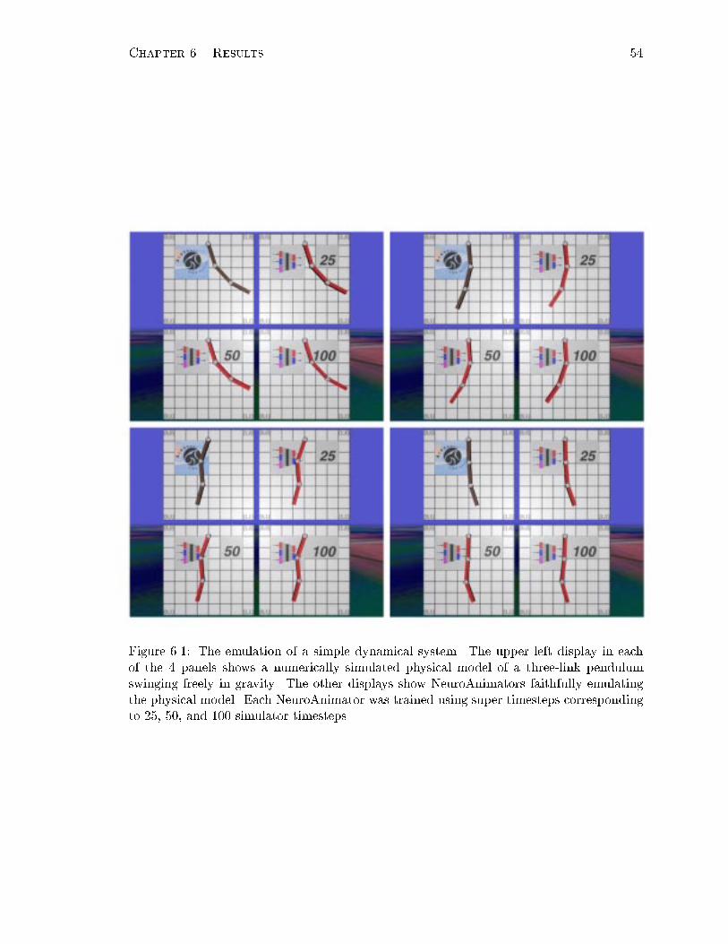
Chapter 6. Results 54

Figure 6.1: The emulation of a simple dynamical system. The upper left display in eachof the 4 panels shows a numerically simulated physical model of a three-link pendulumswinging freely in gravity. The other displays show NeuroAnimators faithfully emulatingthe physical model. Each NeuroAnimator was trained using super timesteps correspondingto 25, 50, and 100 simulator timesteps.


Figure 6.2: Frames from the animation comparing the response of the physical system andits emulator to the same set of control inputs for the case of the space ship. The model onthe left represents the physical system, the model on the right|its emulator.


Figure 6.3: Frames from the animation comparing the response of the physical system andits emulator to the same set of control inputs for the case of the truck. The model on theleft represents the physical system, the model on the right|its emulator.


Figure 6.4: The far dolphin is animated by simulating its biomechanical model which isactuated by internal muscle actions. The near dolphin is animated by a NeuroAnimatorthat emulates the physical model at much less computational cost.


Figure 6.5: Emulated motion produced by training a NeuroAnimator on state transi-tion data generated by the Hodgins mechanical runner model, simulated numerically bySD/FAST. The trained neural network emulator produces this running animation. Thedata used for training the runner was a 30 sec. simulation sequence produced at �t = 0:0027sec. using SD/FAST. From this sequence we generated 11,000 training examples to trainthe networks for the runner model.

Model State Force Control Hidden State Training

Description Inputs Inputs Inputs Units Outputs Examples

Pendulum

passive 6 | | 20 6 2,400

active 6 | 3 20 6 3,000

ext. force 6 3 3 20 6 3,000

Lander 13 | 4 50 13 13,500

Truck 6 | 2 40 6 5,200

Dolphin

global net 78 | 6 50 78 64,000

local net 72 | 6 40 36 32,000

Runner

torso 23 | | 30 23 14,000

arm 12 | | 30 12 7,200

leg 12 | | 30 12 7,200

Table 6.1: Structure of the NeuroAnimators used in our experiments. Columns 2, 3, and 4indicate the input groups of the emulator, column 4 indicates the number of hidden units,and column 5 indicates the number of outputs. The �nal column shows the size of the dataset used to train the model. The dolphin NeuroAnimator includes six local nets, one foreach body segment.


Model Physical N25

�N50

�N100

�N50

�with

Description Simulation Regularization

Passive Pendulum 4.70 0.10 0.05 0.02 |

Active Pendulum 4.52 0.12 0.06 0.03 |

Truck 4.88 | 0.07 | |

Lunar Lander 6.44 | 0.12 | |

Dolphin 63.00 | 0.95 | 2.48

Table 6.2: Comparison of simulation time between the physical simulator and di�erent neu-ral network emulators. The duration of each test was 20,000 physical simulation timesteps.

using SD/FAST to generated 11,000 training examples to train the networks for the runnermodel.

For each experiment, to ensure an unbiased evaluation of the generalization quality ofthe emulators, we use the test data that comprises examples that were not part of thetraining set.

6.1.1 Performance Benchmarks

An important advantage of using neural networks to emulate dynamical systems is the speedat which they can be iterated to produce animation. Since the emulator for a dynamicalsystem with the state vector of size N never uses more than O(N) hidden units, it can beevaluated using only O(N2) operations. Appendix A contains the computer code for theforward step. By comparison, a single simulation timestep using an implicit time integrationscheme requires O(N3) operations.2 Moreover, a forward pass through the neural networkis often equivalent to as many as 50 or 100 physical simulation steps, so the acceleration iseven more dramatic, yielding performance improvements as great as 100 times faster thanthe physical simulator.

In the remainder of this section we use Nn� to denote a neural network model that was

trained with super timestep �t = n�t. Table 6.1.1 compares the physical simulation timesobtained using the SD/FAST physical simulator and 3 di�erent neural network models:N25

� , N50� , and N100

� . The neural network model that predicts over 100 physical simulationsteps o�ers a speedup of anywhere between 50 and 100 times depending on the type of thesystem. In case of the deformable dolphin model, the �rst column indicates the simulationtime using the physical simulator described in (Tu and Terzopoulos, 1994), the third columnshow the simulation time using N50

� emulator, and the last column shows the impact ofregularization on the emulation time. In this case, each emulation step includes 5 iterationof the regularizer described in Section 6.1.3. For the car model and the lunar lander modelwe have trained only the N50

� emulators.

6.1.2 Approximation Error

An interesting property of the neural network emulation, as Fig. 6.6 testi�es, is that theerror does not increase appreciably for emulators with increasingly larger super timesteps;

2Strictly speaking, the implicit numerical methods take O(N3) operations only if all the variables of thephysics-based model depend on each other. Most often, however, the physics-based models are sparselyconnected. If banded matrix techniques are used, then the numerical methods take O(p2N), where p is thebandwidth of the matrix. For non-banded systems, (preconditioned) conjugate gradient can be used. If eachvariable is connected to k others, then conjugate gradient converges in O(kN2).


0 10 20 30 40 50 600

0.05

0.1

0.15

0.2

0.25passive−kinematic chain

time [s]

e(x)

0 10 20 30 40 50 600

0.05

0.1

0.15

0.2

0.25active−kinematic chain

time [s]

e(x)

(a) (b)

Figure 6.6: The error e(x) in the state estimation incurred by di�erent neural networkemulators, measured as the absolute di�erence between the state variables of the emulatorand the associated physical model. Plot (a) compares the approximation error for thepassive pendulum for 3 di�erent emulator networks: N25

� (solid), N50� (dashed), N100

� (dot-dashed). Plot (b) shows the same comparison for the active pendulum. In all experiments,we averaged the error over 30 simulation trials and over all state variables. The durationof each trial was 6000 physical simulation timesteps.

i.e., in the graphs, the error over time for N25� , N50

� , and N100� is nearly the same. This is

attributable to the fact that an emulator network that can predict further into the futuremust be iterated fewer steps per given interval of animation than must an emulator thatcan't predict so far ahead. Thus, although the error per iteration may be higher for thelonger-range emulator, the growth of the error over time can remain nearly the same forboth the longer and shorter range predictors. This means that the only penalty for usingemulators that predict far ahead might be a loss of detail (high frequency componentsin the motion) due to coarse sampling. However, we did not observe this e�ect for thephysical models with which we experimented. This suggests that the physical systems arelocally smooth. Of course, it is not possible to increase the neural network predictiontime inde�nitely, because eventually the network will no longer be able to approximate thephysical system at all adequately.

Although it is hard to totally eliminate error, we noticed that for the purposes of com-puter animation the approximation error remained within reasonable bounds. The neuralnetwork emulation appears comparable to the physical simulation, and although the emu-lated trajectory di�ers slightly from the trajectory produced by the physical simulator, theemulator seems to reproduce all of the visually salient properties of the physical motion.

6.1.3 Regularization of Deformable Models

When emulating spring-mass systems in which the degrees of freedom are subject to softconstraints, we discovered that the modest approximation error of even a well-trained em-ulator network can accumulate as the network is applied repeatedly to generate a lengthy


animation. Unlike an articulated system whose state is represented by joint angles and henceis kinematically constrained to maintain its connectivity, the emulation of mass-spring sys-tems can result in some unnatural deformations after many (hundreds or thousands of)emulation steps. Accumulated error can be annihilated by periodically performing regular-ization steps through application of the true dynamical system (1.1) using an explicit Eulertime integration step

vt+�t = vt + �tf(st);

xt+�t = xt + �tvt+�t;

where the state is st = [vt;xt]T and f(st) is the spring deformation force at time t. It is

important to note that this inexpensive, explicit Euler step is adequate as a regularizer,but it is impractical for long-term physical simulation because of its instability. In order toapply the explicit Euler step we used a smaller spring sti�ness and larger damping factorwhen compared to the semi-explicit Euler step used during the numerical simulation (Tuand Terzopoulos, 1994). Otherwise the system would oscillate too much or would simplybecome unstable.

We achieve the best results when performing a small number of the regularization stepsafter each emulation step. This produces much smoother motion than performing moreregularization step but less frequently. To measure the deformation of the model we de�nethe deformation energy

Ed =1

2

mXi=0

"lci � lrilri

#2

wherem is the number of springs, lci is the current length of spring i, and lri is its rest length.

Fig. 6.7 shows how the regularization reduces the deformation energy of the model. Thesolid line shows the deformation energy of the emulator that follows each emulation stepwith 5 regularization steps. This is enough to keep the deformation approximately constantand roughly at the same level as during the physical simulation. When the emulator doesnot use the regularizer, the deformation energy continuously increases with time.

6.2 Control Learning Results

This section presents results of applying the new control learning algorithm to the trainedNeuroAnimators. The report includes the comparison of the new technique with the controllearning techniques used previously in the computer graphics literature.

We have successfully applied our backpropagation through time controller learning al-gorithm to the trained NeuroAnimators. We �nd the technique very e�ective|it routinelycomputes solutions to non-trivial control problems in just a few iterations.

For example, a swimming controller for the dolphin model was synthesized in just 20learning emulations. The convergence rate is breathtaking compared with control synthe-sis techniques that do not exploit gradient information (van de Panne and Fiume, 1993;Grzeszczuk and Terzopoulos, 1995). In particular, (Grzeszczuk and Terzopoulos, 1995) re-ports that the same swimming controller took 3000 physical simulations to synthesize usingsimulated annealing, and 700 iterations using the simplex method. The e�ciency accruedfrom our fast convergence rate is further ampli�ed by the replacement of costly physicalsimulation with much faster NeuroAnimator emulation. These two factors yield enormous


0

0.05

0.1

0.15

0.2

0.25

0.3

0.35

0.4

0 10 20 30 40 50 60 70 80

defo

rmat

ion

ener

gy

simulation time

’regularize.mat’’noregularize.mat’

’physical.mat’

Figure 6.7: The plot compares deformation energy for 3 di�erent cases: emulation withregularization, emulation without regularization, and physical simulation. The �rst caseperforms 5 regularization steps after each emulation step. This is enough to keep thedeformation energy at the same level as during the physical simulation.

speedups|the synthesis of the swimming controller which took more than 1 hour using thetechnique in (Grzeszczuk and Terzopoulos, 1995) now takes less than 10 seconds on thesame computer.

Fig. 6.8 shows the progress of the control learning algorithm for the 3-link pendulum.The purple pendulum, animated by a NeuroAnimator, has a goal to end the simulationwith zero velocity in the position indicated by the green pendulum. We make the learningproblem very challenging by setting a low upper limit on the internal motor torques of thependulum, so that it cannot reach its target in one shot, but must swing back and forth togain the momentum necessary to reach the goal state. Our algorithm takes 20 iterations tolearn a controller that successfully achieves the goal.

Fig. 6.9 shows the lunar lander NeuroAnimator learning a soft landing maneuver. Thetranslucent lander resting on the surface indicates the desired position and orientation ofthe model at the end of the animation. An additional constraint is that the downwardvelocity upon landing should be small enough to land softly. A successful landing controllerwas computed in 15 learning iterations.

Fig. 6.10 shows the truck NeuroAnimator learning to park. The translucent truck in thebackground indicates the desired position and orientation of the model at the end of thesimulation. The NeuroAnimator produces a parking controller in 15 learning iterations.

Fig. 6.11 shows the dolphin NeuroAnimator learning to swim forward. Simple objec-tive of moving as far forward as possible produces a natural looking, sinusoidal swimmingpattern.

All trained controllers are 20 seconds long, i.e., they take 2,000 physical simulationtimesteps, or 40 emulator super timesteps using N50

� emulator. The number of control


Figure 6.8: Frames from the animation showing progress of the control learning algorithmfor the 3-link pendulum. The purple pendulum representing the emulator has a goal to endthe simulation in the position indicated by the green pendulum at zero velocity.


Figure 6.9: Frames from the animation showing progress of the control learning algorithmfor the space ship. The model resting on the surface of the planet indicates the desiredposition and orientation of the emulator at the end of the simulation. Minimal velocity atlanding constitutes an additional requirement.


Figure 6.10: Frames from the animation showing the truck learning to park. The model farin the background indicates the desired position and orientation of the emulator at the endof the simulation.


Figure 6.11: Frames from the animation showing the dolphin learning to swim. Simple ob-jective of moving as far forward as possible produces a natural looking, sinusoidal swimmingpattern.


variables optimized varies: the pendulum optimizes 60 variables, 20 for each actuator; thelunar lander optimizes 80 variables, 20 for the main thruster, and 20 for each of the 3attitude thrusters; the car optimizes 40 variables|20 for acceleration/deceleration, and 20for the rate of turning; �nally, the dolphin optimizes 60 variables|one variable for every 2emulator steps for each of the six muscles.

6.3 Directed vs Undirected Search in Control Space

This section compares the e�ciency of the gradient directed control learning algorithmproposed in this thesis with the e�ciency of the undirected search techniques presented in(Grzeszczuk and Terzopoulos, 1995).

We use the locomotion learning problem studied in (Grzeszczuk and Terzopoulos, 1995)as the test case for our experiment. In this problem, the dolphin model needs to learn howto actuate its 6 independent muscles over time in order to swim forward e�ciently. The taskis de�ned in terms of the objective function that measures the distance of the model fromsome far away goal. Fig. 6.11 shows the frames from the animation depicting the learningprocess.

Fig. 6.12 reports the results of the experiment for the di�erent algorithm as plots of theprogress of learning as a function of the number of iterations. The plot on the left has beentaken from (Grzeszczuk and Terzopoulos, 1995) and shows the progress of learning usingtwo undirected search methods: simulated annealing and simplex. 3 Plot on the right showsthe result for the gradient directed algorithm. While the older techniques take between 500and 3500 iteration to converge because in the absence of the gradient information theyneed to perform extensive sampling of the control space, the gradient directed algorithmconverges to the same solution in as little as 20 iterations. The use of the neural networkemulator o�ers, therefore, a two orders of magnitude reduction in the number of iterationsand a two orders of magnitude reduction in the execution time of each iteration.

6.3.1 Gradient Descent vs Momentum

Figures 6.13{6.15 compare the convergence of the simple gradient descent and the gradientdescent with the momentum term on the problem of control synthesis. Section 3.4.2 de-scribes in detail the advantage of using the momentum term during the update step. Thetwo methods di�er in the implementation of the update rule.

xl+1 = xl + �xl+1: (6.1)

where the simple gradient descent de�nes �wl+1 as

�xl+1 = ��xrxE� (xl); (6.2)

and the gradient descent with momentum de�nes this term as

�xl+1 = ��xrxE� (xl) + �x�x

l: (6.3)

3In Fig. 6.12, the plot on the left shows the results for the controller de�ned using both global and localbasis functions. The plot on the right that illustrates the progress of learning of the gradient directed searchshows the result for the controller de�ned using the local basis functions only.


0.4

0.5

0.6

0.7

0.8

0.9

1

0 500 1000 1500 2000 2500 3000 3500

objective function

function evaluations

Simplex Method on the Freqency ControllerAnnealling on the Frequency ControllerSimplex Method on the Time Controller

Annealling on the Time Controller

0.4

0.5

0.6

0.7

0.8

0.9

1

0 5 10 15 20

obje

ctiv

e fu

nctio

n


backpropagation through time

Figure 6.12: Convergence rate comparison between the directed and the undirected opti-mization methods on the problem of locomotion learning for the dolphin model. The ploton the left shows the progress of learning for two optimization methods that do not use thegradient information: simulated annealing and the simplex method. The plot on the rightshows the convergence of the algorithm that uses gradient to direct the search. The tech-nique that uses gradient converges in 20 iteration, while the other techniques take between500 and 3500 iterations to �nd the solution.

0

0.2

0.4

0.6

0.8

1

1.2

1.4

0 5 10 15 20

obje

ctiv

e fu

nctio

n



0

0.2

0.4

0.6

0.8

1

1.2

1.4

0 5 10 15 20

obje

ctiv

e fu

nctio

n



Figure 6.13: Progress of learning for the 3-link pendulum problem. The plot on the left wasproduced using the momentum term during, and therefore, converges faster than simplegradient descent shown on the right.

Fig. 6.13 illustrates the progress of learning for the 3-link pendulum control learning problemdescribed in Section 6.2 and shown in Fig. 6.8. The results obtained using the momentumterm are shown in the plot on the left and were generated using the following parameters:�x = 2:0, �x = 0:5. The results obtained using the simple gradient descent are shown in theplot on the right and were generated using �x = 1:2|the largest learning rate that wouldconverge. Clearly, the momentum term decreases the error much more rapidly and permitsa larger learning rate.

Fig. 6.14 illustrates the progress of learning for the lunar lander problem described inSection 6.2 and shown in Fig. 6.9. The results obtained using the momentum term areshown in the plot on the left and were generated using the following parameters: �x = 1:5,�x = 0:5. The results obtained using the simple gradient descent are shown in the plot onthe right and were generated using �x = 1:0|the largest learning rate that would converge.As in the previous example, the momentum term decreases the error much more rapidly


0

0.2

0.4

0.6

0.8

1

1.2

1.4

0 5 10 15 20

obje

ctiv

e fu

nctio

n



0

0.2

0.4

0.6

0.8

1

1.2

1.4

0 5 10 15 20

obje

ctiv

e fu

nctio

n



Figure 6.14: Progress of learning for the landing problem. The plots show the objectiveas a function of the iteration of the control learning algorithm. The plot on the left wasproduced using the momentum term, and therefore, converges faster than simple gradientdescent shown on the right.

0

0.2

0.4

0.6

0.8

1

1.2

1.4

1.6

1.8

2

0 5 10 15 20

obje

ctiv

e fu

nctio

n



0

0.2

0.4

0.6

0.8

1

1.2

1.4

1.6

1.8

2

0 5 10 15 20

obje

ctiv

e fu

nctio

n



Figure 6.15: Progress of learning for the parking problem. The plots show the objectiveas a function of the iteration of the control learning algorithm. The plot on the left wasproduced using the momentum term, and therefore, converges faster than simple gradientdescent shown on the right.

and enables a larger learning rate.Fig. 6.15 illustrates the progress of learning for the parking problem described in Sec-

tion 6.2 and shown in Fig. 6.10. The results obtained using the momentum term are shownin the plot on the left and were generated using the following parameters: �x = 1:5, �x = 0:5.The results obtained using the simple gradient descent are shown in the plot on the rightand were generated using �x = 1:5. Although both strategies use the same learning rate,the momentum term damps the oscillation and therefore converges faster.

Chapter 7

Conclusion and Future Work

7.1 Conclusion

Animation through the numerical simulation of physics-based graphics models o�ers un-surpassed realism, but it can be computationally demanding. Likewise, �nding controllersthat enable physics-based models to produce desired animations usually entails formidablecomputational cost. This thesis demonstrates the possibility of replacing the numericalsimulation and control of model dynamics with a dramatically more e�cient alternative.In particular, we propose the NeuroAnimator, a novel approach to creating physically re-alistic animation that exploits neural networks. NeuroAnimators are automatically trainedo�-line to emulate physical dynamics through the observation of physics-based models inaction. Depending on the model, its neural network emulator can yield physically realisticanimation one or two orders of magnitude faster than conventional numerical simulation.The e�ciency is due to the low cost of the neural network evaluation and the fact that thenetwork can accurately predict a long chain of evaluations of the physical simulator in asingle step. Furthermore, by exploiting the network structure of the NeuroAnimator, we in-troduce a fast algorithm for learning controllers that enables either physics-based models ortheir neural network emulators to synthesize motions satisfying prescribed animation goals.We demonstrate NeuroAnimators for passive and active (actuated) rigid body, articulated,and deformable physics-based models.

To minimize the approximation error of the emulation, we construct a structured Neu-roAnimator that has intrinsic knowledge about the underlying model built into it. Themain subnetwork of the structured NeuroAnimator predicts the state changes of the modelin its local coordinate system. A cascade of smaller subnetworks forms an interface be-tween the main subnetwork and the inputs and outputs of the NeuroAnimator. To limitthe approximation error that accumulates during the emulation of the deformable models,we introduce the regularization step that minimizes the deformation energy.

For complex dynamical systems with large state spaces we introduce hierarchical emu-lators that can be trained much more e�ciently. The networks in the bottom level of thistwo level hierarchy are responsible for the emulation of di�erent subsystems of the model,while the network at the top level of the hierarchy combines the results obtained by thelower level.

Except for very simple cases for which one can derive an analytical description, the phys-ical systems used in computer graphics are not di�erentiable. Controller synthesis withoutgradient information necessitates brute force exploration of the control space that requires

70

Chapter 7. Conclusion and Future Work 71

many costly physical simulations and is therefore painfully slow. However, the NeuroAni-mator forms a di�erentiable model of the underlying physical system and, hence, forms abasis for an e�cient control algorithm that uses the gradient to guide the search throughthe control space. In essence, the algorithm integrates the model over time to predict thefuture result and then di�erentiates the error in the outcome back in time to compute thee�ect of current actions on future results. This strategy proves very e�cient since it replacescostly physical simulation with inexpensive neural emulation, and it synthesizes solutionsto complex control problems in a few iterations by using the gradient.

The heavy computational burden of physical simulation and the lack of suitable controlalgorithms has retarded the penetration of physics-based models into commercial computergraphics systems. The connectionist approach developed in this thesis addresses both ofthese issues simultaneously in a uni�ed fashion. It promises to help make physical realismin computer animation ubiquitous.

A neural network emulation o�ers a convenient handle for trading e�ciency and realism.For example, if we care more for e�ciency than for realism we can approximate the physicalmodel using a network with a reduced number of weights and units, or we can train thenetwork to make larger time steps then the physical simulator. Connectionist emulationtherefore gives the user control over degree of physical realism.

7.2 Future Research Directions

7.2.1 Model Reconstruction

In the future, we foresee neural network emulators, similar to those presented in the disser-tation, �nding applications in the reconstruction of physically realistic models. Suppose, forexample, that we have the training data describing physically correct state transitions of amodel, but not its physical properties, nor the control forces that caused these transitions.The case we have in mind is that of motion capture which certainly produces physicallyrealistic data, but excludes a lot of information about the underlying physical model suchas control and contact forces. Given that the training data has enough diversity, we shouldbe able to compose an emulator for the model underlying the captured data that recoversall its salient physical properties. In fact, we should be able to reconstruct the controllersresponsible for the state transitions in the training data without much di�culty. We thinkthis should be a very interesting line of research.

7.2.2 Emulator Improvements

We want to test the e�ect of using a committee of networks on the generalization qualityof the network. This method trains many di�erent candidate networks and then combinesthem together to form a committee (Perrone, 1993; Perrone and Cooper, 1994). This leadsto signi�cant improvements in generalization, but incurs a performance penalty due to theevaluation of multiple networks during each emulation step.

Yet another approach to improving network generalization we would like to evaluate isthe use of adaptive mixtures of local experts to divide the learning into subtasks, each ofwhich can be solved by a small and e�cient expert network (Jacobs et al., 1991; Jordanand Jacobs, 1994).

Chapter 7. Conclusion and Future Work 72

7.2.3 Neural Controller Representation

In the future, we would like to replace the current controller representation that uses controlvariables to describe a set of control functions with a neural network. The existing controllercan learn to perform only a single control task while the controller network should be ableto learn a variety of them. In fact, it is possible that the controller network trained on arepertoire of simple basic control problems will likely generalize to similar yet di�erent tasks.We hope that the connectionist controller o�ers a su�ciently elaborate representation toenable the emergence of complex behavior. We foresee that a controller network trained on avariety of simple, low-level tasks, such as swimming forward and turning, will automaticallyform an abstraction of controllers that solve higher-level problems, such as target tracking.Furthermore, we believe that the connectionist formulation o�ers uniformity that will makethe interface between the separate control networks much more intelligible and elegant.

7.2.4 Hierarchical Emulation and Control

In the future, as we seek computer models that solve increasingly di�cult tasks requiringextensive planning and taking a long time to execute, we will need to build emulatorsat di�erent temporal scales. Even the best emulators cannot predict the behavior of theunderlying model accurately forever. We foresee that the control for complex tasks willtherefore have to be done hierarchically, where the control algorithm �rst solves the problemat a high level of abstraction described at a coarse temporal level, and then learns to performeach high-level task using low-level actions that take less time to execute.

7.2.5 NeuroAnimators in Arti�cial Life

In recent years, a new computation �eld has emerged, dubbed Arti�cial Life, that seeksto gain a better understanding of complex biological systems through their computer sim-ulation. Biologically inspired models of animals, or animats, have also been of interest tocomputer animators who believe that such models will lead to more realistic results. Thework presented here is of interest to both disciplines since it makes computer models morereactive and life-like through the use of biologically inspired neural networks.

One possible interpretation for the NeuroAnimators, that would be appealing from theArti�cial Life point of view, is that the emulation represents the retrospective mode ofthe animat, while the simulation represents its active mode, and the animat uses theminterchangeably to make better decisions about the future actions. In this scenario, themodel is normally engaged in the execution mode, but breaks occasionally from it in orderto re ect on its actions and plan future behavior. This is an interesting topic for futurework.

Appendix A

Forward Pass Through the

Network

The following is a C++ function for calculating the outputs of a neural network from theinputs. It implements the core loop that takes a single super timestep in an animationsequence with a trained NeuroAnimator.

BasicNet::forwardStep(void)

{

int i,j,k;

double *input = inputLayer.units;

double *hidden = hiddenLayer.units;

double *output = outputLayer.units;

double **ww = inputHiddenWeights;

double **vv = hiddenOutputWeights;

// compute the activity of the hidden layer

for (j=0;j<hiddenSize;j++) {

hidden[j] = biasHiddenWeights[j];

for (i=0;i<inputSize;i++)

hidden[j] += input[i]*ww[i][j];

hidden[j]=hiddenLayer.transFunc(hidden[j]);

}

// compute the activity of the output layer

for (k=0;k<outputSize;k++) {

output[k] = biasOutputWeights[k];

for (j=0;j<hiddenSize;j++)

output[k] += hidden[j]*vv[j][k];

output[k]=outputLayer.transFunc(output[k]);

}

}

73

Appendix B

Weight Update Rule

In Section 3.3.1 we have presented the weight update rule that uses the on-line gradientdescent to train a network to approximate an example set (x� ;y� ). Here we derive ane�cient, recursive implementation of the algorithm that constitutes the essential part ofthe backpropagation algorithm (Rumelhart, Hinton and Williams, 1986). Although thederivation is for a speci�c case of a simple feedforward neural network with one hiddenlayer, we also show how to generalize the algorithm to a feedforward network with anarbitrary topology. Fig. B.1 introduces the notation.

Recall that the algorithm de�nes the network approximation error as

E� (w) = E(x� ;w) = jj�(x� )�N(x� ;w)jj; (B.1)

and it seeks to minimize the objective

E(w) =1

2

nX�=1

E� (w); (B.2)

where n is the number of training examples. The on-line gradient descent implementationof the algorithm adjusts the network weights after each training example k:

wl+1 = wl � �wrwE�(wl) (B.3)

where �w < 1 denotes the weight update learning rate, and l speci�es the iteration of theminimization step.

We derive here an e�cient, recursive rule for computing the derivatives in (B.3). The al-gorithm �rst computes the derivative of the error with respect to the layer of weights directlyadjacent to the outputs, and then uses this result recursively to compute the derivatives withrespect to the earlier layers of weights. The name of the backpropagation algorithm stemsfrom this recursive computation, that in essence propagates the derivative information fromthe network outputs back to its inputs.

We start the derivation by computing the error derivatives with respect to the hidden-to-output connections. Using the chain rule of di�erentiation we get the following expression

@E� (w)

@wjk

=@E� (w)

@yk

@yk@wjk

(B.4)

Applying the chain rule twice, we get a similar expression for the derivatives with respect

74

Chapter B. Weight Update Rule 75

1

hiddenlayer

outputlayer

w01

wqr

yr

y1

inputlayer

vpq

v01

xp

x1

x =10

Figure B.1: Three-layer feedforward neural network N. Bias units are not shaded. xidenotes the activation of input unit i, hj|of hidden unit j, and yk|of output unit k; vijdescribes the weight between input unit i and hidden unit j, and wjk describes the weightbetween hidden unit j and output unit k.

to the input-to-hidden connections

@E� (w)

@vij=

@E� (w)

@hj

@hj@vij

=@hj@vij

rXk=1

@E� (w)

@yk

@yk@hj

(B.5)

All the derivatives occurring on the left side of (B.4) and (B.5) can now be easily calculated.Based on the notation introduced in Fig. B.1, we have the following expressions describingthe activations of hidden and output units

hj = gh(pX

i=1

xivij) = gh(xvj) (B.6)

yk = gy(qX

j=1

hjwjk) = gy(hwk) (B.7)

where gh and gy are respectively the activation functions of the hidden and the output layer.We use these expressions to derive the partial derivatives used in (B.4) and (B.5)

@yk@wjk

= hjg0

y(hwk) (B.8)

@yk@hj

= wjkg0

y(hwk) (B.9)

@hj@vij

= xig0

h(xvj) (B.10)

@hj@xi

= vijg0

h(xvj) (B.11)

where g0h and g0y indicate the derivatives of the activation functions. Assuming that the


approximation error is de�ned as the squared distance between the output of the networkand the desired output and from B.2, we can additionally write

@E� (w)

@yk=

1

2

@(tk � yk)2

@yk= �(tk � yk) = E�

k (B.12)

where tk is the target output for unit k and yk is the true output for this unit. Substituting(B.12) and (B.8) into (B.4) we get the expression for the error derivatives with respect tothe hidden-to-output weights

@E� (w)

@wjk

= E�k � hj � g

0

y(hwk) = hj�k (B.13)

where we have de�ned�k = E�

k � g0

y(hwk) (B.14)

Substituting (B.10), (B.12) and (B.9) into (B.5) we get the expression for the error deriva-tives with respect to the input-to-hidden weights

@E� (w)

@vij= xi � g

0

h(xvj)rX

k=1

E�k � wjk � g

0

y(hwk): (B.15)

Using (B.14), we can rewrite this expression as

@E� (w)

@vij= xi � g

0

h(xvj)rX

k=1

wjk�k = xi�j (B.16)

where we have de�ned

�j = g0h(xvj)rX

k=1

wjk�k (B.17)

Based on (B.3), we can �nally write the on-line gradient descent rule for the hidden-to-output layer

wl+1jk = wl

jk � �whj�k; (B.18)

and for the input-to-hidden layer

vl+1ij = vlij � �wxi�j : (B.19)

Note that both update rules have the same form, and di�er only in the de�nition of �'s.In fact, since (B.17) gives a recursive rule for computing �'s for the given layer of unitsin terms of �'s from the previous layer, update rule (B.19) can be used in a feedforwardnetworks with an arbitrary number of layers. Incremental computation of the derivativesmakes the backpropagation algorithm very e�ciently.

Computation of the derivatives can be further simpli�ed if we take the implementationspeci�cs of an emulator under account. Since the emulator uses the identity function as theinput activation function gx and the output activation function gy, the functions derivatives,g0x and g

0

y, become the identity. Also, the emulator always uses the logistic sigmoid functionas the activation function for the hidden layer, and this function has a useful property thatits derivative can be expressed in terms of the function itself: sig0(x) = sig(x)(1 � sig(x)).


These facts enable us to write (B.17) as

�j = sig0(xvj)rX

k=1

wjk�k = hj(1� hj)rX

k=1

wjk�k; (B.20)

and (B.14) as�k = E�

k � g0

y(hwk) = E�k : (B.21)

Since the new set of update rules reuses unit activations computed during the forward passthrough the network, it makes the backpropagation step simpler and more e�cient.

The following is a C++ function implementing the online version of the weight updaterule. We assume that before executing this function the network has been presented withan input pattern for which there is a known target pattern, and that the activations of thehidden and the output layers were calculated for the network based on this input using thefunction presented in Appendix A. The update rule for the bias weights is the same as forthe other weights.

void

BasicNet::backpropUpdateWeightsStep(void)

{

int i, j, k; double value;

double *input = inputLayer.units;



double *hiddenDelta = hiddenDeltaLayer.units;

double *outputDelta = outputDeltaLayer.units;

double **v = inputHiddenWeights;

double **w = hiddenOutputWeights;

// compute the output layer deltas

for(k=0;k<outputSize;k++) {

outputDelta[k] = -(target[k] - output[k]);

ouputDelta[k] *= outputLayer.transDeriv(output[k]);

}

// update the hidden-to-output weights

for (j=0;j<hiddenSize;j++)

for(k=0;k<outputSize;k++) {

w[j][k] -= learningRate * hidden[j] * outputDelta[k];

biasOutputWeights[k] -= learningRate * outputDelta[k];

}

// compute the hidden layer deltas


hiddenDelta[j] = 0.0;

for(k=0;k<outputSize;k++)

hiddenDelta[j] += w[j][k] * outputDelta[k];


hiddenDelta[j] *= hiddenLayer.transDeriv(hidden[j]);

}

// update the input-to-hidden weights

for(i=0;i<inputSize;i++)


v[i][j] -= learningRate * input[i] * hiddenDelta[j];

biasHiddenWeights[j] -= learningRate * hiddenDelta[j];

}

Appendix C

Input Update Rule

In Section 3.3.2 we have presented the input update rule that uses the on-line gradient de-scent to alter the control inputs of the network in order to achieve the desired output. Thisalgorithm forms an essential part of the controller synthesis process described in Chapter 5.The input update rule di�ers from the traditional version of the backpropagation algo-rithm (Rumelhart, Hinton and Williams, 1986) in that it adjusts the inputs while keepingthe weights constant. However, the essential philosophy of the backpropagation algorithmstays intact. For this reason, there is a signi�cant overlap between the weight updaterule (Appendix B) and the rule described here. Both derivations share the same notationintroduced in Fig. B.1.

Recall that the algorithm seek to minimize the objective de�ned as

E(x) = jjNd �N(x)jj2 (C.1)

where Nd denotes the desired output of the network. We can rewrite E as

E(x) =1

2

rXk=1

(tk � yk)2 =

rXk=1

Ek (C.2)

The on-line gradient descent implementation of the algorithm adjusts the network inputsusing the following rule

xl+1 = xl � �xrxE(xl) (C.3)

where �x < 1 denotes the input update learning rate, and l describes the iteration of theoptimization step.

We derive here an e�cient, recursive rule for computing the derivatives in (C.3). Ap-plying the chain rule of di�erentiation twice to the equation we get

@E

@xi=

rXk=1

@Ek

@xi=

rXk=1

@Ek

@yk

@yk@xi

=rX

k=1

@Ek

@yk

qXj=1

@yk@hj

@hj@xi

(C.4)

We rearrange the terms to get

@E

@xi=

qXj=1

rXk=1

@Ek

@yk

@yk@hj

@hj@xi

=qX

j=1

@hj@xi

rXk=1

@Ek

@yk

@yk@hj

(C.5)

Note that the bias units, which receive constant input signals and have therefore zero

79

Chapter C. Input Update Rule 80

gradient, have been excluded from the summation term. Using (B.9) and (B.11), we simplifythe notation by introducing the following expressions

�k =@Ek

@yk= �(tk � yk)

�j =rX

k=1

�k@yk@hj

=rX

k=1

�k � wjk � g0

y(hwk)

�i =qX

j=1

�j@hj@xi

=qX

j=1

�j � vij � g0

h(xvj)

Based on (C.3), we can now write a very concise representation of the on-line gradientdescent rule for the ith input unit

xl+1i = xli � �x�i (C.6)

Since the rule for the input �'s is de�ned recursively in terms of the �'s in the previouslayers, the input update rule (C.6) can be used to compute the derivatives in a feedforwardnetwork with an arbitrary number of layers.

We use the logistic sigmoid function as the activation function for the hidden layerand the identity function for both the input and the output layer. The logistic sigmoidfunction has the property that its derivative can be expressed in terms of the functionitself: sig0(x) = sig(x)(1 � sig(x)). These facts enable us to simplify the expression for �s

�j =rX

k=1

�k � wjk � g0

y(hwk) =rX

k=1

�k � wjk

�i =qX

j=1

�j � vij � g0

h(xvj) =qX

j=1

�j � vij � hj(1� hj)

This makes the backpropagation step easier to implement and more e�cient, because wecan evaluate the input adjustments using solely the unit activations computed during theforward pass through the network.

The following is a C++ function implementing the online version of the input updaterule. We assume that before executing this function the network has been presented withan input pattern for which there is a known target pattern, and that the activations of thehidden and the output layers were calculated for the network based on this input using thefunction presented in Appendix A.

void

BasicNet::backpropInputsUpdateRule(void)

{

int i, j, k; double value;



double *inputDelta = inputDeltaLayer.units;

double *hiddenDelta = hiddenDeltaLayer.units;

double *outputDelta = outputDeltaLayer.units;

Chapter C. Input Update Rule 81

// compute the deltas for the output layer ( output deltas

// depend on the definition of the error function)

setOutputDeltas();

// compute the deltas for the hidden layer


hiddenDelta[j] = 0.0;

for (k=0;k<outputSize;k++) {

value = hiddenOutputWeights[j][k]*outputLayer.transDeriv(output[k]);

value *= outputDelta[k];

hiddenDelta[j] += value;

}

}

// compute the deltas for the input layer

for (i=0;i<inputSize;i++) {

inputDelta[i] = 0.0;


value = inputHiddenWeights[i][j]*hiddenLayer.transDeriv(hidden[j]);

value *= hiddenDelta[j];

inputDelta[i] += value;

}

}

// update the inputs to the network

for (i=0;i<inputSize;i++)

inputs[i] += learningRate*inputDelta[i];

}

Appendix D

Quaternions

A quaternion can represent an arbitrary 3D rotation using only four parameters, and ro-tation interpolation in the quaternion space is simple and smooth. These two propertiesmake the quaternion encoding of rotation a better choice then its two alternatives: theEuler angles and the rotation matrix. The Euler angles, such as yaw, pitch, and roll, can-not represent an arbitrary rotation because of the singularity that occurs when the tworotations axes collapse into one. The rotation matrix, on the other hand, requires as manyas nine parameters to encode the rotation and the interpolation of two rotation matricescannot be performed directly.

For the reasons outlined above we choose to represent the joint orientations of a rigid-body using quaternions. However, the emulation and the control learning using quaternionsrequires a distinct set of operations. Speci�cally, to compute the change in the orientationof the model, we need to be able to subtract two quaternion rotations. We also need to knowhow to interpolate smoothly between two joint orientations represented as quaternions toobtain the motion of the model in-between the super timesteps. Finally, for the purposes ofbackpropagation through time we need to know how to di�erentiate operations that involvequaternions.

This appendix reviews the quaternion algebra related to our work. First we introducethe quaternion notation as presented in the paper by Hart et al. (Hart, Francis and Kauf-mann, 1994). This includes a matrix representation for quaternion multiplication usedby the emulation step. Subsequently, we review quaternion interpolation as presented in(Shoemake, 1985). Finally, we derive the quaternion multiplication di�erentiation step, andintroduce the quaternion rotation error measure used to evaluate of the objective function.

D.1 Quaternion Representation

A quaternion q = r + xi + yj + zk = r + v consists of a real part r and a pure partv = xi+ yj+ zk. Vectors i, j, k signify the three-dimensional vectors

i = (1; 0; 0); (D.1)

j = (0; 1; 0); (D.2)

k = (0; 0; 1): (D.3)

82

Chapter D. Quaternions 83

Let q1 = r1 + v1 and q2 = r2 + v2 be the two quaternions. Their sum is

q1 + q2 = (r1 + r2) + (v1 + v2); (D.4)

and their product is

q1q2 = r1r2 + v1 � v2 + r1v2 + r2v1 + v1 � v2: (D.5)

The magnitude of q is de�ned as

kqk =pr2 + v � v:

Let q = a + bu be a quaternion such that kuk = 1 is the imaginary unit three-vector. Itsconjugate is �q = a� bu, and its magnitude is

kqk = q�q =pa2 + b2: (D.6)

Any quaternion q = a+ v can be represented as q = a+ bu through the relation

u =x

kvki+

y

kvkj+

z

kvkk: (D.7)

D.2 Quaternion Rotation

Rotations are represented by unit quaternions, i.e., the quaternions of unit magnitude.Shoemake (Shoemake, 1985) represents a rotation of � about the axis u as

q = cos1

2� + sin

1

2�u: (D.8)

Hart et al. employ the notation used in engineering sciences, that represents a complexnumber of unit magnitude as ei� = cos � + i sin �, to produce a very compact quaternionrepresentation

q = e1

2�u: (D.9)

D.2.1 Rotation Negation

From (D.6) it follows that to invert a unit quaternion, we simply negate its pure part

q�1 = �q: (D.10)

D.2.2 Rotation Summation

We multiply two quaternions to sum the rotations that they represent, analogously to theoperation done on the rotation matrices

e1

2�u = e

1

2�1u1 � e

1

2�2u2 = q1q2 (D.11)

where the multiplication is done according to the rule (D.5). Note, that it is much moree�cient to add rotations represented as quaternions then it is when they are representedusing rotation matrices.


D.3 Rotation Interpolation

Linear interpolation of two rotations, q1 and q2, requires that the rotation changes at aconstant speed. Shoemake showed that this can be done by interpolating on the unit sphere,along the great circle arc between the two rotations. He gives the following formula for thespherical linear interpolation from q1 to q2, with parameter u moving from 0 to 1

slerp(q1;q2; u) =sin(1� u)�

sin �q1 +

sinu�

sin �q2; (D.12)

where q1 � q2 = cos �:

D.4 Matrix Representation of Quaternion Multiplication

The structured emulator introduced in Section 4.3 computes the joint orientation !t+�t byadding two quaternion rotations: !t and �!t through quaternion multiplication accordingto the rule(D.5). However, for the purposes of a connectionist implementation it is far moreconvenient to represent quaternion multiplication in a matrix form that we present here.

Let q1 = [ qr1 qx1 qy1 q

z1 ] and q2 = [ qr2 q

x2 qy2 q

z2 ] represent two quaternion rotations, and

let q = [ qr qx qy qz ] be the product of q1 and q2. Expanding the multiplication rule (D.5)we get the following set of equations

qr = qr1qr2 � qx1q

x2 � qy1q

y2 � qz1q

z2

qx = qr1qx2 + qx1q

r2 + qy1q

z2 � qz1q

y2

qy = qr1qy2 + qy1q

r2 + qz1q

x2 � qx1q

z2

qz = qr1qz2 + qz1q

r2 + qx1q

y2 � qy1q

x2

(D.13)

which can be written concisely in a matrix form

q = q1q2 = Q1q2 =

26664

qr1 �qx1 �qy1 �qz1qx1 qr1 qz1 �qy1qy1 �qz1 qr1 qx1qz1 qy1 �qx1 qr1

3777526664qr2qx2qy2qz2

37775 : (D.14)

D.5 Di�erentiation of Quaternion Rotation

Since the emulation step performs quaternion multiplication, the backpropagation controllearning algorithm needs to compute the derivative of the output rotation q with respectto the input quaternions q1 and q2. We use the expanded version of the quaternion multi-plication (D.13) to compute the Jacobian of q with respect to q1

@q

@q1=

26664

qr2 �qx2 �qy2 �qz2qx2 qr2 qz2 �qy2qy2 �qz2 qr2 qx2qz2 qy2 �qx2 qr2

37775 (D.15)


and with respect to q2

@q

@q2=

26664qr1 �qx1 �qy1 �qz1qx1 qr1 �qz1 qy1qy1 qz1 qr1 �qx1qz1 �qy1 qx1 qr1

37775 : (D.16)

D.6 Orientation Error Metric in Quaternion Space

Since the control learning algorithm computes the error at the end of an emulation basedon the state of the model, we need to be able to determine what this error is for theorientation de�ned as a quaternion. Let qM+1 be the orientation of the model at the endof the emulation, and let qd = [ qrd q

xd qyd q

zd ] be the desired orientation of the model at this

point. We de�ne the orientation error as

ER =1

2(qu � qo)

2: (D.17)

where qu = [ 1 0 0 0 ] is the quaternion with zero rotation, and qo = q�qd. Using thechain rule of di�erentiation, we obtain the following expression for the derivative of ER

with respect to q@ER

@q=

@ER

@qo

@qo@q

(D.18)

where@ER

@qo= [qro � qru; q

xo � qxu; q

yo � qyu; q

zo � qzu] (D.19)

and

@qo@q

=

26664

�qrd ��qxd ��qyd ��qzd�qxd �qrd �qzd ��qyd�qyd ��qzd �qrd �qxd�qzd �qyd ��qxd �qrd

37775 : (D.20)

Appendix E

Description of the Models

This appendix describes the physical models used as the emulator prototypes. For the rigidbodies we include the SD/FAST script used to build the model and the forces computationfunction used by the physical simulator.

E.1 Multi-Link Pendulum

The following is an SD/FAST script used to generate the equations of motion for the three-link pendulum shown in Fig. 6.1. The model has 3 links|link0 attaches to the ground,link1 attaches to link0, and �nally link2 attaches to link1. The links connect through thepin joints that rotate around the y-axis. There is a gravity force acting on the model.

E.1.1 SD/FAST Script

gravity = 0 0 -9.8

body = link0 inb = ground joint = pin

mass = 1 inertia = 5 0 0 0 5 0 0 0 1

bodytojoint = 0 0 0.25 inbtojoint = 0 0 0

pin = 0 1 0

body = link1 inb = link0 joint = pin

mass = 1 inertia = 5 0 0 0 5 0 0 0 1

bodytojoint = 0 0 0.25 inbtojoint = 0 0 -0.25

pin = 0 1 0

body = link2 inb = link1 joint = pin

mass = 1 inertia = 5 0 0 0 5 0 0 0 1

bodytojoint = 0 0 0.25 inbtojoint = 0 0 -0.25

pin = 0 1 0

E.1.2 Force Computation Function

The following is a C function for calculating the external torques acting on the joints of themodel. Each torque is a sum of the control force and the friction force that depends on theangular velocity of the joint.

86

Chapter E. Description of the Models 87

Figure E.1: The geometrical model of the lunar lander. Underlying it is a physical modelthat can rotate freely in 3D.

void sduforce(double time, double *pos, double *vel)

{

int i; double torque;

// loop through all the joints

for (i=0;i<jointCount;i++) {

// compute the torque

torque = controlForce[i] - frictionCoef*vel[i];

// apply the torque to the joint

sdhinget(i,0,torque);

}

}

E.2 Lunar Lander

The following is an SD/FAST script used to generate the equations of motion for the lunarlander model shown in Fig. E.1. Physical representation of the model consists of a rigidblock that can rotate freely in 3D. The model has 4 internal controls|the main jet thatpropels the lander, and 3 orthogonal thrusters that change the orientation of the model.



body = ship inb = ground joint = sixdof

mass = 100.0

inertia = 5 0 0 0 5 0 0 0 2

bodytojoint = 0 -1 0.0 inbtojoint = 0 0 0

pin = 1 0 0

pin = 0 1 0

pin = 0 0 1


extern int globalControlCount;

extern double* globalControls;

The following is a C function for calculating the external torques

acting on the joints of the model. Each torque is a sum of the control

force and the friction force that depends on the angular velocity of

the joint.


{

// jet positions

double shipPos[3] = { 0.0, 0.0, 0.0};

double jet0[3] = { 0.25, 0.0, 0.0};

double jet1[3] = {-0.25, 0.0, 0.0};

// jet forces

double mainJet[3] = {0.0,0.0,10.0};

double azim0[3] = { 0.0, 0.5, 0.0};

double azim1[3] = { 0.0,-0.5, 0.0};

double incl0[3] = { 0.0, 0.0, 0.5};

double incl1[3] = { 0.0, 0.0,-0.5};

mainJet[2] *= globalControls[0];

azim0[1] *= globalControls[1];

azim1[1] *= globalControls[1];

incl0[2] *= globalControls[2];

incl1[2] *= globalControls[2];

// apply the main jet force

sdpointf(0,shipPos,mainJet);

// apply the orientation jets

sdpointf(0,jet0,azim0);

sdpointf(0,jet0,incl0);


sdpointf(0,jet1,azim1);

sdpointf(0,jet1,incl1);

// apply linear friction force

double linIn[3], linOut[3];

for (int i=0;i<3;i++) {

linIn[i] = -0.2*vel[i];

}

sdtrans(-1,linIn,0,linOut);

sdpointf(0,shipPos,linOut);

// apply angular friction force

double angIn[3], angOut[3];

for (i=0;i<3;i++) {

angIn[i] = -0.2*vel[i+3];

}

sdbodyt(0,angIn);

}

E.3 Truck

The following is an SD/FAST script used to generate the equations of motion for the truckmodel shown in Fig. E.2. Physical representation of the model consists of a rigid block thatcan slide on the plane z = 0, and rotate around the z axis. The model can exert two typesof forces|one that accelerates/decelerates in the forward direction, and one that changesthe orientation of the model.


body = block inb = ground joint = planar

mass = 100.0

inertia = 5 0 0 0 5 0 0 0 2

bodytojoint = 0 -1 0 inbtojoint = 0 0 0.25

pin = 1 0 0

pin = 0 1 0

pin = 0 0 1


extern int globalControlCount;

extern double* globalControls;


{

// change the orientation

double stearPos[3] = { 0.0, 2.0, 0.0};

// stearing forces

double stear[3] = { 2.0, 0.0, 0.0};


Figure E.2: The geometrical model of the truck. Underlying it is a physical model thatconsists of a rigid block that can slide on the plane z = 0, and rotate around the z axis.


stear[0] *= globalControls[0];

// apply the acceleration force

sdpointf(0,stearPos,stear);

Vector <double> forwardVec(0,1,0);

Vector <double> sideVec(1,0,0);

// get the car orientation

double dircos[3][3];

sdorient(0,dircos);

Matrix3 orientMat(dircos);

// convert the vectors to WCS

forwardVec = orientMat*forwardVec;

sideVec = orientMat*sideVec;

// find the joint velocity in WCS

double jointPos[3]; double absVel[3];

sdgetbtj(0,jointPos);

sdvel(0,jointPos,absVel);

Vector <double> absVelVec; absVelVec.setVec(absVel);

// compute the gas acceleration

double gas[3] = { 0.0, 10.0, 0.0};

gas[1] *= globalControls[1];

// apply the aceleration force

sdpointf(0,jointPos,gas);

double force[3], forceOut[3];

// compute the sideways friction

double sideFactor = -200.0*sideVec.dot(absVelVec);

Vector <double> sideForce(sideVec);

sideForce *= sideFactor;

sideForce.getVec(force);

sdtrans(-1,force,0,forceOut);

sdpointf(0,jointPos,forceOut);

// compute the forward friction

double forwardFactor = -0.2*forwardVec.dot(absVelVec);

Vector <double> forwardForce(forwardVec);

forwardForce *= forwardFactor;

forwardForce.getVec(force);

sdtrans(-1,force,0,forceOut);

sdpointf(0,jointPos,forceOut);

}


E.4 Dolphin

E.4.1 Spring-Mass Model

The biomechanical model of the dolphin is constructed of nodal masses and springs, as isdetailed in Fig. E.3. The model's dynamics is speci�ed by the Lagrangian equations ofmotion

mi�xi + i _xi +Xj2Ni

f sij = fi (E.1)

where node i has mass mi, position xi(t) = [xi(t); yi(t); zi(t)], velocity _x, and dampingfactor i, and where fi is an external force. Spring Sij , which connects node i to neighboringnodes j 2 Ni, exerts the force f

sij(t) = �(cijeij + ij _eij)rij=jjrij jj on node i (and it exerts

the force �f sij on node j), where cij is the elastic constant, ij is the damping constant, andeij(t) = jjrij jj � lij is the deformation of the spring with separation vector rij(t) = xj � xi.The natural length of the spring is lij .

Some of the springs in the biomechanical model play the role of contractile muscles.Muscles contract as their natural length lij decreases under the autonomous control of themotor center of the arti�cial animal's brain (Tu and Terzopoulos, 1994). To dynamicallycontract a muscle, the brain must supply an activation function a(t) to the muscle. Thiscontinuous time function has range [0; 1], with 0 corresponding to a fully relaxed muscle oflength lrij and 1 to a fully contracted muscle of length lcij . More speci�cally, for a musclespring, lij = alcij + (1� a)lrij .


12

34

56

Figure E.3: The geometrical model of the dolphin (top) and the underlying biomechanicalmodel (bottom). The model has six actuators consisting of a pair of muscles that share thesame activation function. The numbers along the body indicate the local centers of massused for building the hierarchical emulator. The cross-springs that maintain the structuralintegrity of the body have not been indicated.

Appendix F

Example Xerion Script

Section 4.3 proposed a special NeuroAnimator structure that minimizes the emulation ap-proximation error. Fig. 4.4 shows the architecture of the structured NeuroAnimator thattransforms the inputs to N� using a sequence of prede�ned transformations before feed-ing the signal through the specialized network N�

�. The following is a Xerion script thatspeci�es and trains the network N�

� used to build the NeuroAnimator for the lunar landermodel described in Section E.2 and shown in Fig. E.1.

#! /u/xerion/uts/bin/bp_sh

# The network has 13 inputs, 50 hidden units, and

# 13 outputs. The hidden layer uses the logistic

# sigmoid as the activation function (default).

uts_simpleNet landerNet 13 50 13

bp_groupType landerNet.Hidden {HIDDEN DPROD LOGISTIC}

# Initialize the example set. Read

# the training data from a file.

set trainSet "landerNet.data"

uts_exampleSet $trainSet

uts_loadExamples $trainSet landerNet.data

# Randomize the weights in the network.

random seed 3

uts_randomizeNet landerNet

# Initialize the minimizer and tell it to use

# the network and the training set defined above.

bp_netMinimizer mz

mz configure -net landerNet -exampleSet trainSet

# Start the training and save the weights

# of the network after the training is finished.

mz run

uts_saveWeights landerNet landerNet.weights

94

Chapter F. Example Xerion Script 95

#---End of script---

F.1 Training Data

This section describes the conversion process that produces training data in the formatrequired by the structured emulator. The example uses the physical model of the lunarlander described in Section E.2. Its state consists of four groups s = [p q v !] where p =[px py pz] describes the position, q = [qr qx qy qz] describes the orientation, v = [vx vy vz]describes the linear velocity, and ! = [!x !y !z] describes the angular velocity. The modelhas 4 internal actuators represented as u = [u1 u2 u3 u4]. The training data collectedduring the physical simulation of the model is represented in the format suitable for theinput/output structure of the NeuroAnimator N�:

fpqv! ugt1 fpqv! ugt1+�t

fpqv! ugt2 fpqv! ugt2+�t

...

fpqv! ugtn fpqv! ugtn+�t

However, to train the structured emulator described in Section 4.3, the training data need tobe transformed to a di�erent format, suitable for the input/output structure of the subnetN�

�. Section 4.5.2 describes the data conversion process, and Fig. 4.13 illustrates the idea.As a result of the conversion, the original set of inputs x undergoes the following trans-

formationx� = T�

xT0

xx (F.1)

while the original set of outputs y is transformed through

y� = (T�yT

0

yT�y )

�1y: (F.2)

The reader should note that the transformations applied to the input groups pt and qtproduce zero vectors as output. Based on the facts that = T0

xpt = RTt (pt � ct) and

pt = ct, it follows that T0

xpt = [0 0 0]. Similarly, from the facts that T0

xqt = QTt qt and

QTt qt = �qtq = [1 0 0 0], it follows that T0

xqt = [1 0 0 0]. Since there is no need to supplyconstant values as inputs to the network, the �nal form of the transformed training datalooks as follows:

fv� !� u�gt1 fp� q� v� !� u�gt1+�t

fv� !� u�gt2 fp� q� v� !� u�gt2+�t

...

fv� !� u�gtn fp� q� v� !� u�gtn+�t

Appendix G

Controller Representation

Discrete-time neural network emulation (4.1) requires discretization of the controller u(t).We parameterize the controller through discretization using basis functions. Mathemati-cally, we express the ith control function as a B-spline

ui(t) =MXj=1

ujiBj(t); (G.1)

where the uji are scalar parameters and the Bj(t), 1 � j �M are (vector-valued) temporalbasis functions. Backpropagation through time, used for control learning, constraints usto use local controller discretization, for which the parameters uji are nodal variables andthe Bj(t) can be spline basis functions.1 In a typical discretization the control variables donot span more than one super timestep �t, which is often equivalent to 50 simulation timesteps �t.

We use the Catmull-Rom family of splines to generate control functions that smoothlyinterpolate the control points (Catmull and Clark, 1974). We choose a member of thisfamily for which the tangent vector at point uji is parallel to the line connecting points u

j�1i

and uj+1i , as shown in Figure G. The representation for the jth segment of the ith controlfunction is

uji (t) =1

2�ht3 t2 t 1

i26664�1 3 �3 12 �5 4 �1

�1 0 1 00 2 0 0

3777526664uj�1i

ujiuj+1i

uj+2i

37775 :

For the �rst segment of the curve u1i (t) we make u0i = u1i , i.e., we duplicate the �rstcontrol point of each control function. Similarly, for the last segment of the curve uM�1

i (t)we make uM+1

i = uMi , i.e., we duplicate the last control point of each control function.

1In our earlier work (Grzeszczuk and Terzopoulos, 1995), we proposed global controller discretization,for which the support of the Bj(t) covers the entire temporal domain t0 � t � t1. We abandon this repre-sentation in this work since globally discretized controllers are not suitable for the current implementationof the control learning algorithm.

96

Chapter G. Controller Representation 97

u i2 u i

3 u i4 u =ui

M−1u iM−2u i

1u =i0

iM

Figure G.1: A Catmull-Rom spline. The points are interpolated by the spline. Indicatedby the straight line is the direction of the curve at each point. The direction is parallel tothe line connecting two adjacent points. To extend the spline to the boundary points weduplicate the �rst and last points.

REFERENCES 98

References

Albus, J. S. (1975). A new approach to manipulator control: The cerebellar model artic-ulation controller (cmac). Transactions of the ASME Journal of Dynamic Systems,

Measurements, and Control, 97:220{227.

Anderson, C. W. (1987). Strategy learning with multilayer connectionist representations.In Proceedings of the Fourth International Workshop on Machine Learning, pages 103{114.

Armstrong, W. W. and Green, M. (1985). The dynamics of articulated rigid bodies forpurposes of animation. In Wein, M. and Kidd, E. M., editors, Graphics Interface '85

Proceedings, pages 407{415. Canadian Inf. Process. Soc.

Atkeson, C. G. and Reinkensmeyer, D. J. (1988). Using associative content-addressablememories to control robots. In Proceedings of the IEEE Conference on Decision andControl, pages 792{797, Austin, Tx.

Badler, N. I., Barsky, B. A., and Zeltzer, D., editors (1991). Animation from instructions,pages 51{93. Morgan Kaufmann.

Bara�, D. (1989). Analytical methods for dynamic simulation of non-penetrating rigid bod-ies. In Lane, J., editor, Computer Graphics (SIGGRAPH '89 Proceedings), volume 23,pages 223{232.

Barto, A. G. (1990). Connectionist learning for control: An overview. In Miller, W. T.,Sutton, R. S., and Werbos, P. J., editors, Neural Networks for Control, pages 5{58.The MIT Press.

Barto, A. G. and Jordan, M. I. (1987). Gradient following without back-propagation inlayered networks. In Caudill, M. and Butler, C., editors, Proceedings of the IEEE

First Annual Conference on Neural Networks, pages II629{II636, San Diego, CA. SOSPrinting.

Barto, A. G., Sutton, R. S., and Anderson, C. W. (1983). Neuronlike adaptive elements thatcan solve di�cult learning control problems. IEEE Transactions on Systems, Man, and

Cybernetics, 13(5):834{846.

Barzel, R. and Barr, A. H. (1988). A modeling system based on dynamic constraints. InDill, J., editor, Computer Graphics (SIGGRAPH '88 Proceedings), volume 22, pages179{188.

Bishop, C. M. (1995). Neural Networks for Pattern Recognition. Clarendon Press.

Brooks, R. (1991). Intelligence without representation. Arti�cial Intelligence, 47:139{159.

Brotman, L. S. and Netravali, A. N. (1988). Motion interpolation by optimal control. InDill, J., editor, Computer Graphics (SIGGRAPH '88 Proceedings), volume 22, pages309{315.

Bruderlin, A. and Williams, L. (1995). Motion signal processing. In Cook, R., editor,SIGGRAPH 95 Conference Proceedings, Annual Conference Series, pages 97{104. ACMSIGGRAPH, Addison Wesley. held in Los Angeles, California, 06-11 August 1995.

REFERENCES 99

Bryson, A. E. and Ho, Y.-C. (1969). Applied Optimal Control. Blaisdell, New York.

Carignan, M., Yang, Y., Thalmann, N. M., and Thalmann, D. (1992). Dressing animatedsynthetic actors with complex deformable clothes. In Catmull, E. E., editor, Computer

Graphics (SIGGRAPH '92 Proceedings), volume 26, pages 99{104.

Catmull, E. E. and Clark, J. H. (1974). A class of local interpolating splines. In Barnhill,R. E. and Riesenfeld, R. F., editors, Computer Aided Geometric Design, pages 317{326.Academic Press, New York.

Cohen, M. F. (1992). Interactive spacetime control for animation. In Catmull, E. E., editor,Computer Graphics (SIGGRAPH '92 Proceedings), volume 26, pages 293{302.

Cybenko, G. (1989). Approximation by superposition of sigmoidal function. Mathematics

of Control Signals and Systems, 2(4):303{314.

Dennis, J. E. and Schnabel, R. B. (1983). Numerical Methods for Unconstrained Optimiza-tion and Nonlinear Equations. Prentice-Hall, Englewood Cli�s, NJ.

Desbrun, M. and Gascuel, M. (1995). Animating soft substances with implicit surfaces. InCook, R., editor, SIGGRAPH 95 Conference Proceedings, Annual Conference Series,pages 287{290. ACM SIGGRAPH, Addison Wesley. held in Los Angeles, California,06-11 August 1995.

Duda, R. O. and Hart, P. E. (1973). Pattern Classi�cation and Scene Analysis. Wiley, NewYork.

Fletcher, R. (1987). Practical Methods for Optimization. John Wiley, New York, secondedition.

Foley, J. D., van Dam, A., Feiner, S. K., and Hughes, J. F. (1990). Computer Graphics,

Principles and Practice, Second Edition. Addison-Wesley, Reading, Massachusetts.Overview of research to date.

Foster, N. and Metaxas, D. (1997). Modeling the motion of a hot, turbulent gas. InWhitted,T., editor, SIGGRAPH 97 Conference Proceedings, Annual Conference Series, pages181{188. ACM SIGGRAPH, Addison Wesley. ISBN 0-89791-896-7.

Gill, P. E., Murray, W., and Wright, M. H. (1981). Practical Optimization. Academic Press,London.

Goh, C. J. and Teo, K. L. (1988). Control parameterization: A uni�ed approach to optimalcontrol problems with general constraints. Automatica, 24:3{18.

Grossberg, S. and Kuperstein, M. (1986). Neural dynamic of adaptive sensory-motor con-

trol: Ballistic eye movements. Elsevier, Amsterdam.

Grzeszczuk, R. and Terzopoulos, D. (1995). Automated learning of Muscle-Actuated loco-motion through control abstraction. In Cook, R., editor, SIGGRAPH 95 Conference

Proceedings, Annual Conference Series, pages 63{70. ACM SIGGRAPH, Addison Wes-ley. held in Los Angeles, California, 06-11 August 1995.

REFERENCES 100

Guenter, B., Rose, C. F., Bodenheimer, B., and Cohen, M. F. (1996). E�cient generationof motion transitions using spacetime constraints. In Rushmeier, H., editor, SIG-GRAPH 96 Conference Proceedings, Annual Conference Series, pages 147{154. ACMSIGGRAPH, Addison Wesley. held in New Orleans, Louisiana, 04-09 August 1996.

Hahn, J. K. (1988). Realistic animation of rigid bodies. In Dill, J., editor, Computer


Hart, J. C., Francis, G. K., and Kaufmann, L. H. (1994). Visualizing quaternion rotation.ACM Transactions on Graphics, 13(3):256{276.

Hertz, J., Krogh, A., and Palmer, R. G. (1991). Introduction to the Theory of Neural

Computation. Addison-Wesley.

Hinton, G. E. (1989). Connectionist learning procedures. Arti�cial Intelligence, 40:185{234.

Hodgins, J. K., Wooten, W. L., Brogan, D. C., and O'Brien, J. F. (1995). Animating humanathletics. In Cook, R., editor, SIGGRAPH 95 Conference Proceedings, Annual Con-ference Series, pages 71{78. ACM SIGGRAPH, Addison Wesley. held in Los Angeles,California, 06-11 August 1995.

Hornik, K., Stinchcomb, M., and White, H. (1989). Multilayer feedforward networks areuniversal approximators. Neural Networks, 2:359{366.

Isaacs, P. M. and Cohen, M. F. (1987). Controlling dynamic simulation with kinematic con-straints, behavior functions and inverse dynamics. In Stone, M. C., editor, Computer


Jacobs, R., Jordan, M. I., Nowlan, S. J., and Hinton, G. E. (1991). Adaptive mixtures oflocal experts. Neural Computation, 3:79{87.

Jordan, M. I. (1988). Supervised learning and systems with excess degrees of freedom. Tech-nical Report 88-27, University of Massachusetts, Computer and Information Sciences,Amherst, MA.

Jordan, M. I. and Jacobs, R. A. (1994). Hierarchical mixture of experts and the em algo-rithm. Neural Computation, 6(2):181{214.

Jordan, M. I. and Rumelhart, D. E. (1992). Supervised learning with a distal teacher.Cognitive Science, 16:307{354.

Kass, M. and Miller, G. (1990). Rapid, stable uid dynamics for computer graphics. InBaskett, F., editor, Computer Graphics (SIGGRAPH '90 Proceedings), volume 24,pages 49{57.

Kawato, M., Setoyama, T., and Suzuki, R. (1988). Feedback error learning of movementby multi-layer neural network. In Proceedings of the International Neural NetworksSociety First Annual Meeting.

Kuperstein, M. (1987). Adaptive visual-motor coordination in multi-joint robots usingparallel architecture. In IEEE International Conference on Robotics and Automation,pages 1595{1602.

REFERENCES 101

Lamouret, A. and van de Panne, M. (1996). Motion synthesis by example. In Proceedings ofthe 7th Eurographics Workshop on Simulation and Animation, pages 199{212, Poitiers,France. Springer Verlag.

Lapedes, A. and Farber, R. (1987). Nonlinear signal processing using neural networks.Technical Report LA-UR-87-2662, Los Alamos National Laboratory, Los Alamos, NM.

Lasseter, J. (1987). Principles of traditional animation applied to 3D computer animation.In Stone, M. C., editor, Computer Graphics (SIGGRAPH '87 Proceedings), volume 21,pages 35{44.

LeCun, Y., Boser, B., Denker, J. S., Henderson, D., Howard, R. E., Hubbard, W., andJackel, L. (1989). Backpropagation applied to handwritten zip code recognition. NeuralComputation, 1(4):541{551.

Lee, Y., Terzopoulos, D., and Waters, K. (1995). Realistic face modeling for animation. InCook, R., editor, SIGGRAPH 95 Conference Proceedings, Annual Conference Series,pages 55{62. ACM SIGGRAPH, Addison Wesley. held in Los Angeles, California,06-11 August 1995.

Liu, Z., Gortler, S. J., and Cohen, M. F. (1994). Hierarchical spacetime control. In Glass-ner, A., editor, Proceedings of SIGGRAPH '94 (Orlando, Florida, July 24{29, 1994),Computer Graphics Proceedings, Annual Conference Series, pages 35{42. ACM SIG-GRAPH, ACM Press. ISBN 0-89791-667-0.

Luenberger, D. G. (1984). Linear and Nonlinear Programming. Addison-Wesley, Reading,MA, second edition.

McKenna, M. and Zeltzer, D. (1990). Dynamic simulation of autonomous legged loco-motion. In Baskett, F., editor, Computer Graphics (SIGGRAPH '90 Proceedings),volume 24, pages 29{38.

Mendel, J. M. and McLaren, R. W. (1970). Reinforcement learning control and patternrecognition systems. In Mendel, J. M. and Fu, K. S., editors, Adaptive, learning and

pattern recognition systems: Theory and applications, pages 287{318. Academic Press,New York.

Miller, G. S. P. (1988). The motion dynamics of snakes and worms. In Dill, J., editor,Computer Graphics (SIGGRAPH '88 Proceedings), volume 22, pages 169{178.

Miller, W. T., Glanz, F. H., and Kraft, L. G. (1987). Applications of a general learningalgorithm to the control of robotic manipulators. International Journal of Robotics

Research, 6:84{96.

Minsky, M. L. and Papert, S. A. (1969). Perceptrons. MIT Press, Cambridge, MA. Ex-panded Edition 1990.

Moody, J. and Darken, C. J. (1989). Fast learning in networks of locally-tuned processingunits. Neural Computation, 1:281{294.

Narendra, K. S. and Parthasarathy, K. (1991). Gradient methods for the optimization of dy-namical systems containing neural networks. IEEE Transactions on Neural Networks,2(2):252{262.

REFERENCES 102

Ngo, J. T. and Marks, J. (1993). Spacetime constraints revisited. In Kajiya, J. T., editor,Computer Graphics (SIGGRAPH '93 Proceedings), volume 27, pages 343{350.

Nguyen, D. and Widrow, B. (1989). The truck backer-upper: An example of self-learningin neural networks. In Proceedings of the International Joint Conference on Neural

Networks, volume 2, pages 357{363. IEEE Press.

Pandy, M. G., Anderson, F. C., and Hull, D. G. (1992). A parameter optimization approachfor the optimal control of large-scale musculoskeletal systems. Transactions of the

ASME, 114(450).

Parker, D. B. (1985). Learning logic. Technical Report TR-47, MIT Center for Researchin Computational Economics and Menagement Science, Cambridge, MA.

Perrone, M. P. (1993). General averaging results for convex optimization. In Mozer, M. C.,editor, Proceedings 1993 Connectionist Models Summer School, pages 364{371, Hills-dale, NJ. Lawrence Erlbaum.

Perrone, M. P. and Cooper, L. N. (1994). When networks disagree: ensamble methods forhybrid neural networks. In Mammone, R. J., editor, Arti�cial Neural Networks for

Speech and Vision, pages 126{142. Chapman and Hall, London.

Platt, J. C. and Barr, A. H. (1988). Constraint methods for exible models. In Dill, J.,editor, Computer Graphics (SIGGRAPH '88 Proceedings), volume 22, pages 279{288.

Polak, E. (1971). Computational Methods for Optimization: A Uni�ed Approach. AcademicPress, New York.

Raibert, M. H. and Hodgins, J. K. (1991). Animation of dynamic legged locomotion.In Sederberg, T. W., editor, Computer Graphics (SIGGRAPH '91 Proceedings), vol-ume 25, pages 349{358.

Ridsdale, G. (1990). Connectionist modeling of skill dynamics. Journal of Visualization

and Computer Animation, 1(2):66{72.

Rosenblatt, F. (1962). Principles of Neurodynamics: Perceptrons and the Theory of Brain

Mechanisms. Spartan, Washington, DC.

Rumelhart, D. E., Hinton, G. E., and Williams, R. J. (1986). Learning internal repre-sentations by error backpropagation. In Rumelhart, D. E., McCleland, J. L., andthe PDP Research Group, editors, Parallel Distributed Processing: Explorations in the

Microstructure of Cognition, volume 1, pages 318{362. MIT Press.

Shoemake, K. (1985). Animating rotation with quaternion curves. In Barsky, B. A., editor,Computer Graphics (SIGGRAPH '85 Proceedings), volume 19, pages 245{254.

Sims, K. (1994). Evolving virtual creatures. In Glassner, A., editor, Proceedings of SIG-

GRAPH '94 (Orlando, Florida, July 24{29, 1994), Computer Graphics Proceedings,Annual Conference Series, pages 15{22. ACM SIGGRAPH, ACM Press. ISBN 0-89791-667-0.

Stam, J. and Fiume, E. (1993). Turbulent wind �elds for gaseous phenomena. In Kajiya,J. T., editor, Computer Graphics (SIGGRAPH '93 Proceedings), volume 27, pages369{376.

REFERENCES 103

Stewart, A. J. and Cremer, J. F. (1992). Beyond keyframing: An algorithmic approach toanimation. In Proceedings of Graphics Interface '92, pages 273{281.

Sutton, R. S. (1984). Temporal credit assignment in reinforcement learning. PhD thesis,University of Massachusetts, Amherst.

Terzopoulos, D. and Fleischer, K. (1988). Deformable models. The Visual Computer,4(6):306{331.

Terzopoulos, D., Platt, J., Barr, A., and Fleischer, K. (1987). Elastically deformable models.In Stone, M. C., editor, Computer Graphics (SIGGRAPH '87 Proceedings), volume 21,pages 205{214.

Terzopoulos, D. and Waters, K. (1990). Physically-based facial modelling, analysis, andanimation. Visualization and Computer Animation, 1:73{80.

Tu, X. and Terzopoulos, D. (1994). Arti�cial �shes: Physics, locomotion, perception, be-havior. In Glassner, A., editor, Proceedings of SIGGRAPH '94 (Orlando, Florida,

July 24{29, 1994), Computer Graphics Proceedings, Annual Conference Series, pages43{50. ACM SIGGRAPH, ACM Press. ISBN 0-89791-667-0.

Unuma, M., Anjyo, K., and Takeuchi, R. (1995). Fourier principles for emotion-basedhuman �gure animation. In Cook, R., editor, SIGGRAPH 95 Conference Proceedings,Annual Conference Series, pages 91{96. ACM SIGGRAPH, Addison Wesley. held inLos Angeles, California, 06-11 August 1995.

van de Panne, M. (1996). Parameteterized gait synthesis. In IEEE Computer Graphics

And Applications, volume 16, pages 40{49.

van de Panne, M. and Fiume, E. (1993). Sensor-actuator networks. In Kajiya, J. T., editor,Computer Graphics (SIGGRAPH '93 Proceedings), volume 27, pages 335{342.

Weigend, A. S. and Gershenfeld, N. A. (1994). Time series prediction: Forecasting thefuture and understanding the past. In Santa Fe Institute Studies in the Science of

Complexity. Santa Fe Institute.

Wejchert, J. and Haumann, D. (1991). Animation aerodynamics. In Sederberg, T. W.,editor, Computer Graphics (SIGGRAPH '91 Proceedings), volume 25, pages 19{22.

Werbos, P. J. (1974). Beyond regression: new tools for prediction and analysis in the

behavioral sciences. PhD thesis, Harvard University, Boston, MA.

Werbos, P. J. (1988). Generalization of back propagation with applications to a recurrentgas market model. Neural Networks, 1:339{356.

Werbos, P. J. (1990). A menu of designs for reinforcement learning over time. In Miller,W. T., Sutton, R. S., and Werbos, P. J., editors, Neural Networks for Control, pages67{95. The MIT Press.

Widrow, B. (1986). Adaptive inverse control. In Second IFAC Workshop on Adaptive

Systems in Control and Signal Processing, pages 1{5, Lund, Sweden. Lund Institute ofTechnology.

REFERENCES 104

Widrow, B. and Lehr, M. A. (1990). 30 years of adaptive neural networks: perceptron,madeline, and backpropagation. In Proceedings of the IEEE, volume 78, pages 1415{1442.

Widrow, B., McCool, J., and Medo�, B. (1978). Adaptive control by inverse modeling. InTwelfth Asilomar Conference on Circuits, Systems, and Computers.

Wilhelms, J. (1987). Using dynamic analysis for realistic animation of articulated bodies.IEEE Computer Graphics and Applications, 7(6):12{27.

Williams, R. J. (1988). On the use of backpropagation in associative reinforcement learning.In Proceedings of the IEEE International Conference on Neural Networks, pages 263{270, San Diego, CA.

Witkin, A. and Kass, M. (1988). Spacetime constraints. In Dill, J., editor, Computer


Witkin, A. and Popovi�c, Z. (1995). Motion warping. In Cook, R., editor, SIGGRAPH 95

Conference Proceedings, Annual Conference Series, pages 105{108. ACM SIGGRAPH,Addison Wesley. held in Los Angeles, California, 06-11 August 1995.

Witkin, A. and Welch, W. (1990). Fast animation and control of nonrigid structures. InBaskett, F., editor, Computer Graphics (SIGGRAPH '90 Proceedings), volume 24,pages 243{252.

Yu, Q. (1998). Synthetic motion capture for interactive virtual worlds. Master's thesis,University of Toronto.

Documents

Abstract - CS | Computer Science