Crime and Social Interactions - Princeton Universityjoses/pp/crime.pdf · CRIME AND SOCIAL INTERACTIONS* ... The media trumpet the large rise in crime since the 1960s, ... crime levels

CRIME AND SOCIAL INTERACTIONS*

EDWARD L. GLAESER BRUCE SACERDOTE

Jost A. SCHEINKMAN

The high variance of crime rates across time and space is one of the oldest puzzles in the social sciences; this variance appears too high to be explained by changes in the exogenous costs and benefits of crime. We present a model where social interactions create enough covariance across individuals to explain the high cross-city variance of crime rates. This model provides an index of social interactions which suggests that the amount of social interactions is highest in petty crimes, moderate in more serious crimes, and almost negligible in murder and rape.

Quelquefois aussi le crime prend sa source dans l'esprit d'imitation, que l'homme possede 'a un haut degre et qu'il manifeste en toutes choses [A. Quetelet 1835].

I. INTRODUCTION

The most puzzling aspect of crime is not its overall level nor the relationships between it and either deterrence or economic opportunity.' Rather, following Quetelet [1835], we believe that the most intriguing aspect of crime is its astoundingly high variance across time and space. The media trumpet the large rise in crime since the 1960s, but there are also cases where criminal activity has fallen dramatically over time. From 1933 to 1961 homicide rates dropped in half the United States. Lane [1979] documents an equally substantial drop in homicides in Philadelphia over the late nineteenth century.

The large intertemporal differences in crime rates are dwarfed by the differences in crime across space. Homicide rates across nations range from 6.1 homicides per million in Japan, to 12.6 homicides per million in Sweden, to 98.0 homicides per mil-

*The National Science Foundation provided generous financial support. Gary Becker, John Cochrane, Glenn Ellison, Lars Hansen, Caroline Minter Hoxby, Hide Ichimura, Guido Imbens, Richard Posner, Adriano Rampini, Jesus Santos, two anonymous referees, and especially Lawrence Katz provided helpful suggestions. Julie Khaslavsky, Andrei Scheinkman, and Jake Vigdor provided excellent research assistance.

1. In part, these topics are less puzzling to us because of the extensive work since Becker [1968] that has been done on them, e.g., Ehrlich [1975], Levitt [1994], and Freeman [1991]. Wilson and Herrnstein [1980] provide an introduction to the broader crime literatures.

? 1996 by the President and Fellows of Harvard College and the Massachusetts Institute of Technology. The Quarterly Journal of Economics, May 1996.

508 QUARTERLY JOURNAL OF ECONOMICS

lion in the United States in 1990. Within the United States cities range from 0.008 serious crimes per capita for Ridgewood Village, New Jersey, to 0.384 serious crimes per capita for nearby Atlantic City.2 Even within a single city, the diversity across subcity units can be astounding; the 123rd precinct of New York City has 0.022 serious crimes per capita, while the 1st precinct had 0.21 crimes per capita.

An obvious explanation for these high variances is that economic and social conditions also vary over space. But even casual empiricism suggests that differences in observable local area characteristics can account for little of the variation in crime rates over space. East Point, Georgia, has a crime rate of 0.092 crimes per capita. El Dorado, Arkansas, which has more unemployment, less education, more poverty, and lower per capita income, has a crime rate of 0.039 crimes per capita. The 51st precinct of New York City has 0.046 crimes per capita while the wealthier 49th precinct has 0.116 crimes per capita. How can the radical differences in the crime rates of these areas be accounted for by their underlying economies? More rigorously, we generally find that less than 30 percent of the variation in cross-city or cross-precinct crime rates can be explained by differences in local area attributes.

Positive covariance across agents' decisions about crime is the only explanation for variance in crime rates higher than the variance predicted by differences in local conditions. When one agent's decision to become a criminal positively affects his neighbor's decision to enter a life of crime, then cities' crime rates will differ from the rates predicted by the cities' characteristics, and those crime rates will differ substantially across locations and over time. Our empirical results are consistent with the existence of these positive interactions.3

To make sense of the covariance across agents that we find in the data, we build on the previous work on social interactions and crime (e.g., Sah [1991], and Murphy, Shleifer, and Vishny [1993]). In our model, agents are arranged on a lattice, and agents' decisions about crime are a function of their own attributes and of their neighbors' decisions about criminal activities.4

2. Atlantic City's crime rate is particularly high because its population does not include much of the large tourist population.

3. Our work supports Case and Katz [1991] who find interactions in a survey of Boston youth.

4. These models are based on the voter models (see Kindermann and Snell [1980]). For other economic models with local interactions, see Scheinkman and Woodford [1994].

CRIME AND SOCIAL INTERACTIONS 509

There are two classes of agents: (1) agents who influence and are influenced by their neighbors; and (2) agents who influence their neighbors, but who cannot themselves be influenced ("fixed agents"). In the model, the variance of crime rates (times the square root of population) is a multiple of the variance of crime rates (times the square root of population) that one would expect if all individuals make independent decisions. The multiple connecting the two variances is a nonlinear, declining function of the proportion of agents who are fixed.

The proportion of the population that is fixed is a parameter of the model that can be estimated using the variance of crime rates. This proportion provides us with an index of the degree of social interactions. We can use this index to ask how the level of social interaction changes across crimes or over time. The number of fixed agents can be interpreted in several ways: the expected distance between two fixed agents is the expected size of a group with positive social interactions, so the number of fixed agents determines the average social group size. Fixed agents can be viewed as agents who do not observe their neighbors' actions, so the number of fixed agents may reflect the share of the population that is not connected to their neighbors; and the number of fixed agents can be seen as a metaphor for the forces that slow social interaction, such as strong parents, formal schooling, or any information that counters peer influence.

The empirical section of the study presents this index of interactions for a variety of different crimes in the United States in 1985, in 1970, and across New York City in 1985. We attempt to control for local conditions first by controlling for a battery of city- level characteristics and in some cases a one-year lag of the city crime rate. We then allow for unobservables in two ways: we assume that unobservables explain twice as much as the one-year lag of the crime rate, and we assume a functional form for unobserved heterogeneity and use that functional form to estimate the variance of unobserved attributes. We also allow for repeat offenders. While we believe our work represents a considerable attempt to correct for unmeasured city level characteristics, we admit that there is considerable uncertainty as to how much of the cross-city variance is actually explained by urban characteristics.

In all three samples we find a high degree of social interaction for larceny and auto theft. Our data show moderate (but still large) levels of interaction for assault, burglary, and robbery. There are very low levels of social interaction for arson, murder,


and rape. Overall, we find that the levels of interaction are similar across the three samples. We believe that this similarity (which does not hold for the mean levels of these crimes) supports the usefulness and reliability of our methodology.

We can use this index across crimes and across cities to try to assess what factors contribute to high levels of social interaction. Across crimes, crimes committed by younger people have higher degrees of social interaction. Across cities, for serious crimes in general, for larceny, and for auto theft, the degree of social interactions is larger in those communities where families are less intact. A possible policy implication is that large reductions in crime levels can be achieved by lowering the degree of social interaction among potentially criminal groups.

As a test of our methodology, we apply it to a variety of data on mortalities from diseases and suicide. For deaths from cancer, diabetes, pneumonia, and suicide, we find extremely small estimated levels of social interaction. Deaths from heart disease display somewhat more social interaction, but still much less interaction than most crimes. Our methodology, in principle, can be used to test for cross-individual effects in many variables beyond crime.

II. PREVIOUS LITERATURE ON POSITIVE INTERACTIONS

The importance of social interactions in forming tastes and actions has long been stressed by sociologists (e.g., Weber [1978] and Simmel [1971]). Among criminologists, Sutherland [1939] is usually credited as being the intellectual ancestor of the differen- tial association school, which emphasizes the importance of social interactions. One natural source of social interaction occurs among criminals acting together; Reiss [1988] surveys the literature on co-offenders. His own work [Reiss 1980] shows that two- thirds of all crimes are committed by offenders acting alone, but two-thirds of all criminals commit crimes jointly. Reiss [1988] lists studies that document how peer interactions operate in the recruitment of young criminals and how peer groups create high crime levels by stigmatizing law-abiding behavior.

Descriptive work often provides the most vivid evidence on the importance of social interactions in motivating criminal behavior. Adler [1995] describes the origin of Detroit's largest crack dealership as stemming from a conversation between Billie Joe Chambers and an old friend and mentor who counseled "BJ, why


don't you start selling crack? ... Crack, man, is cocaine and you make millions of dollars from it." Social interactions seem to create a sense of invulnerability and a willingness to violate social norms and take risks, as long as one is in the company of like- minded individuals. Bing [1991] quotes a young criminal, Bopete, as saying "but when I'm with my homeboys, I don't think of dyin' never at all. Only when I'm alone." Jankowski [1991] gives a particularly rich description of the wide range of social interactions involved in joining gangs.

A number of models already connect positive interactions across criminals with the fact that seemingly identical cities can have different levels of crime. Sah [1991] presents a benchmark model where any one individual's choice to become a criminal lowers the probability that any other individual will be arrested. Police cannot arrest more than a fixed number of criminals, so when there is more crime, the probability of being arrested goes down. Two (or more) equilibria can result: one equilibrium with high crime levels and low probabilities of arrest, and the other equilibrium with low crime levels and a high probability of arrest.

Murphy, Shleifer, and Vishny [1993] suggest an alternative mechanism to create multiple equilibria where high levels of criminal behavior crowd out legal activities. As the number of criminals rises, the returns from not being a criminal fall because legal revenues are stolen by criminals. Alternatively, if noncriminals monitor criminals,5 or decide on the resources to be spent on crime prevention, then as the number of noncriminals falls, the money spent fighting crime also falls, and crime pays a little more. If crime is stigmatizing, then as the number of criminals rises, the average criminal becomes a "normal" member of society. As the stigma from crime falls, it becomes more attractive to commit crimes (see Rasmussen [1995]). Stigma may also create multiple equilibria if crime stigmatizes an area and makes outside employers less likely to hire the residents of a particular city; that lack of hiring then lowers the cost and increases the quantity of crime in the area.6

5. Jacobs [1961] suggests the critical role of civilian monitoring in limiting urban crime. Akerlof and Yellen [1994] focus on community enforcement and gang behavior.

6. There are also negative interactions, most classically standard competi- tion for a scarce resource (victims) means that more criminals lower the returns to criminal activity. These negative interactions would lower, not raise, the observed variance of crime rates.


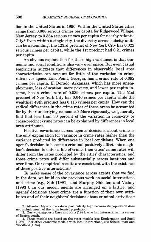
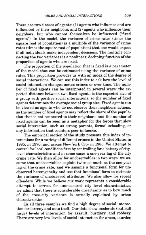
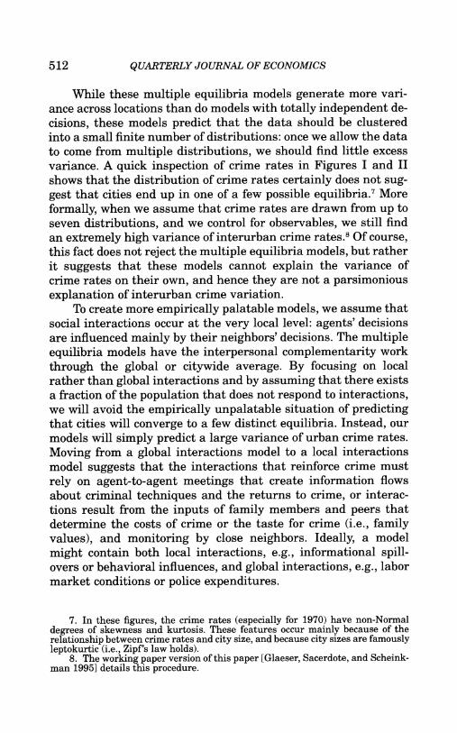
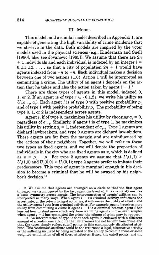
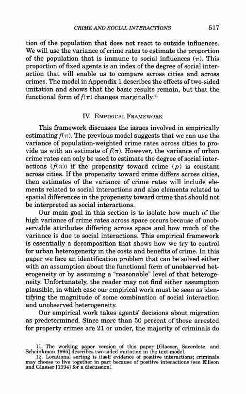
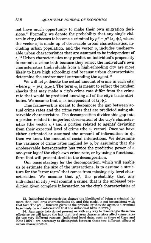
While these multiple equilibria models generate more variance across locations than do models with totally independent decisions, these models predict that the data should be clustered into a small finite number of distributions: once we allow the data to come from multiple distributions, we should find little excess variance. A quick inspection of crime rates in Figures I and II shows that the distribution of crime rates certainly does not suggest that cities end up in one of a few possible equilibria.7 More formally, when we assume that crime rates are drawn from up to seven distributions, and we control for observables, we still find an extremely high variance of interurban crime rates.8 Of course, this fact does not reject the multiple equilibria models, but rather it suggests that these models cannot explain the variance of crime rates on their own, and hence they are not a parsimonious explanation of interurban crime variation.

To create more empirically palatable models, we assume that social interactions occur at the very local level: agents' decisions are influenced mainly by their neighbors' decisions. The multiple equilibria models have the interpersonal complementarity work through the global or citywide average. By focusing on local rather than global interactions and by assuming that there exists a fraction of the population that does not respond to interactions, we will avoid the empirically unpalatable situation of predicting that cities will converge to a few distinct equilibria. Instead, our models will simply predict a large variance of urban crime rates. Moving from a global interactions model to a local interactions model suggests that the interactions that reinforce crime must rely on agent-to-agent meetings that create information flows about criminal techniques and the returns to crime, or interactions result from the inputs of family members and peers that determine the costs of crime or the taste for crime (i.e., family values), and monitoring by close neighbors. Ideally, a model might contain both local interactions, e.g., informational spillovers or behavioral influences, and global interactions, e.g., labor market conditions or police expenditures.

7. In these figures, the crime rates (especially for 1970) have non-Normal degrees of skewness and kurtosis. These features occur mainly because of the relationship between crime rates and city size, and because city sizes are famously leptokurtic (i.e., Zipf's law holds).

8. The working paper version of this paper [Glaeser, Sacerdote, and Scheink- man 1995] details this procedure.


Cross City Crime Rates, 1985

70

60 -

50

40

'3 0 ~~~~~~.. .. .. .. .... ......_

20

0 00 0 0 0 0 0 :. :. : .::: : :::..:. : .

Serious Crimes Per Capita

FIGURE I Serious Crimes per Capita, 1985 U. S. Data

NYC Precinct Crime Rates, 1993

20

18

16 ... .. ... ..

.. . . . . .. ........ .. . . . . _ : : : ,: :. .: . : : :.:.:. :: ... ,:

:: : : ::: ::::: , :[:: : : ::::

... ::: ::. : .....

14

. . . . ~~. . . .. . ... . . . . . . . . . .

lo ~ ~ Seiu Crimes .e ..... 195U.S Ot

20 . ~~~~~~..... ......

......1.. .. h .~~~~~~~~...... .r.-. .. .- . .- .. . I . . . H ~ ~ ~ ~ ~ ~ ~ ~~.. ... ... ::::....::::

0 . .... ..... . 0 .- N Y LtN. Y.... ...... .. ..

1 n

~~~~~~~..... ... .-.-.. ...... ..-.-.-.

i..... s ..... ..... ...C a _ :::::: ::::::::: ::::..... ..... ..;.. . .1 . =

Q ~~~~~~~...... .... . ..... ..... .......

~~~~~~... . ...... ...................... .. .. .......-.. .................. ..... ....

I......... ......... ~~~~~~~~~~~. . . . . . . . . . . . . . . .-.---- J ~~~~.-.-.-.-.. .... -.-.-.-.-.-.-.-.-.-.-.-.-4 .-.-.-.-.1

...... .-.-. .-.- .-...-. .-.-.-.-. -.-.-.-..

.. . . . . . ...... ... . .....

FIGURE II Serious Crimes per Capita, 1993 New York Data


III. MODEL

This model, and a similar model described in Appendix 1, are capable of generating the high variability of crime incidence that we observe in the data. Both models are inspired by the voter models used in the physical sciences (e.g., Kinderman and Snell [1980]; also see Jovanovic [1985]). We assume that there are 2n + 1 individuals and each individual is indexed by an integer i = 0 + 1_+2 ... , so that a city of population 2n + 1 would have agents indexed from -n to +n. Each individual makes a decision between one of two actions {1,0}. Action 1 will be interpreted as committing a crime. The utility of an agent i depends on the action that he takes and also the action taken by agent i - 1.9

There are three types of agents in this model, indexed 0, 1, or 2. If an agent is of type T E {0,1,2}, we write his utility as UT(ai-, at). Each agent i is of type 0 with positive probability po and of type 1 with positive probability pl. The probability of being type 0, 1, or 2 is independent across agents.

Agent i, if of type 0, maximizes his utility by choosing ai = 0, regardless of ait,. Similarly, if agent i is of type 1, he maximizes his utility by setting ai = 1, independent of ail. Type 1 agents are diehard lawbreakers, and type 0 agents are diehard law-abiders. These agents are far from the margin and are uninfluenced by the actions of their neighbors. Together, we will refer to these two types as fixed agents, and we will denote the proportion of individuals in the city who are fixed agents as a, which is defined as 7r = po + pl. For type 2 agents we assume that U2(1,1) > U2(1,0) and U2(0,0) > U2(0,1); type 2 agents prefer to imitate their predecessors. This type of agent is marginal enough in his decision to become a criminal that he will be swayed by his neighbor's decision.'0

9. We assume that agents are arranged on a circle so that the first agent (indexed -n) is influenced by the last agent (indexed n); this circularity ensures a basic symmetry across agents. The interconnection of agents' utilities can be interpreted in many ways. When agent i - l's criminal activity influences the arrest rate, or the return to legal activities, it influences the utility of agent i and the utility agent i gets from criminal activities. For example, agent i receives more utility from committing a crime if agent i - 1 is a criminal because agent i has learned how to steal more effectively from watching agent i - 1 or even simpler when agent i - 1 has committed the crime, the stigma of crime may be reduced.

10. An interpretation of type is that each agent is endowed with a different amount of a continuous attribute that determines the net benefit from crime and that the types simply reflect cutoff points in this continuously distributed attribute. This continuous attribute could be the returns to a legal, alternative activity or the suffering incurred by being arrested or the ability to commit crime or some weighted combination of all of these attributes. Hence, the cutoff points, and the


Each agent observes the action chosen by his predecessor. There is a unique Nash equilibrium given the types of each agent: all strings of type 2 agents that are uninterrupted by type 0 or type 1 agents will imitate the action of the type 1 or type 0 agent that began the string. If there are 1000 type 2 agents in sequence all following a type 1 agent, then all 1001 agents will choose action 1. The remainder of this section examines the distribution of these Nash equilibria across cities.

If each agent's action, denoted ai, is thought of as a random variable that assumes the values of 0 or 1, then the process {ai, -oo < i < oo} is stationary, and the expected value of any ai equals P- P1/(& + p1). The presence of fixed agents of type 0 and 1, who are both independent in their own decisions and serve to create a degree of independence between type 2 agents, guarantees enough "mixing" so that central limit behavior can be estab- lished. More precisely, we know that agent i and agentj are independent conditional on the existence of an agent of type 0 or 1 in the segment [j + 1, i ]. The probability that there is no such agent in that interval goes to zero exponentially as i - j -4 oo. Hence the stationary process {ai, -00 < i < oo} satisfies a strong mixing condition with exponentially declining bounds (cf. Hall and Heide [1980], p. 132) and central limit behavior results. We denote

(1) Sn= a P__

( 1) l~~~~~~il-n 2n + 1)

which means that Sn is the deviation between the expected number of crimes and the realized number of crimes for all individuals i for whom Jil ? n, divided by the total number of individuals for whom Jil ? n. Then,

(2) lim(2n + 1)E(S2) = limE((Sn 2n + 1)2)

noo ~ ~~~ no

n

= var(ao) + 2Dim E cov(aoad). n-+O i=1

probabilities PO and p1, may depend on some city characteristics. In fact, urban characteristics will jointly determine the unconditional probability of committing a crime (p) and . For example, higher employment levels will induce more agents who are always law-abiders and fewer agents who are always lawbreakers, since the opportunity cost of crime has risen. The population percentage p will fall. However, the number of influenceable agents may rise or fall depending on whether the rise in law-abiders (who were presumably formally influenceable agents) outweighs the fall in lawbreakers (who will now become influenceable agents).


As the size of this group grows large, the variance of per capita outcomes weighted by the square root of the group size converges to the unconditional variance of an individual's outcome (var(a0)) plus a term based on the correlation of individuals' actions within the group (21im Xn cov(a0, ai)). The covariance

term cov(aoai) represents the covariance between any individual's action and the action of another individual where the two individuals are separated by exactly i - 1 others. Since ao follows a binomial distribution, var(ao) = p(l - p). To compute the covariance terms in (2), let A be the event that at least one agent in the segment [1,i] is of the type 0 or 1. Conditional on event A occurring, a, is independent of a0, since ai is determined exclu- sively by the value taken by the agent of type 0 or 1 in [1,i]. If A does not occur, ao and ai have the same value and are therefore perfectly correlated. The probability that A does not occur is given by (1 - po - pl)i. Using these facts, we write

n var(ao) + 21im E cov(ao, ai)

n-o i=1 n

=p(l - p) + 21im p(1 -p)(1 -po -pi) n-o i~=1

= p(l - p) + 2p(1 p) (-p0 -p p)

=p(l -p) =0 2

'r

In the last step of equation (3) we are just defining U2 = (p(l - p)

(2 - ir)/rr). Since -rr> 0, 0 < a2 < oo, central limit behavior results (see Hall and Heide [1980, Corollary 5.1, p. 132]), and we know that

(4) S F2n + 1 -*N[O, a2].

We will occasionally refer to (2 - ur)/lr as f(rr). This term represents the covariance across agents and captures the degree of imitation. If no type 2 agents are present, then rr = 1, f(-rr) equals 1, and U2 = p(l - p). As the probability that each agent is of type 2 approaches one (i.e., rr approaches zero), f(rr) and U2 both approach oo. Moreover, as the covariances are decaying exponentially the variance of the left-hand side of (3) converges to a2 at the rate at least 1/n.

The variance of crime rates (times the square root of population) across cities equals p (1 - p) times a function of the propor-


tion of the population that does not react to outside influences. We will use the variance of crime rates to estimate the proportion of the population that is immune to social influences (IT). This proportion of fixed agents is an index of the degree of social interaction that will enable us to compare across cities and across crimes. The model in Appendix 1 describes the effects of two-sided imitation and shows that the basic results remain, but that the functional form of f(Ir) changes marginally.11

IV. EMPIRICAL FRAMEWORK

This framework discusses the issues involved in empirically estimating f(7r). The previous model suggests that we can use the variance of population-weighted crime rates across cities to provide us with an estimate of f(ul). However, the variance of urban crime rates can only be used to estimate the degree of social interactions (ftrr)) if the propensity toward crime (p) is constant across cities. If the propensity toward crime differs across cities, then estimates of the variance of crime rates will include elements related to social interactions and also elements related to spatial differences in the propensity toward crime that should not be interpreted as social interactions.

Our main goal in this section is to isolate how much of the high variance of crime rates across space occurs because of unobservable attributes differing across space and how much of the variance is due to social interactions. This empirical framework is essentially a decomposition that shows how we try to control for urban heterogeneity in the costs and benefits of crime. In this paper we face an identification problem that can be solved either with an assumption about the functional form of unobserved heterogeneity or by assuming a "reasonable" level of that heterogeneity. Unfortunately, the reader may not find either assumption plausible, in which case our empirical work must be seen as iden- tifying the magnitude of some combination of social interaction and unobserved heterogeneity.

Our empirical work takes agents' decisions about migration as predetermined. Since more than 50 percent of those arrested for property crimes are 21 or under, the majority of criminals do

11. The working paper version of this paper [Glaeser, Sacerdote, and Scheinkman 1995] describes two-sided imitation in the text model.

12. Locational sorting is itself evidence of positive interactions; criminals may choose to live together in part because of positive interactions (see Ellison and Glaeser [1994] for a discussion).


not have much opportunity to make their own migration decisions.12 Formally, we denote the probability that any single citi- zen in cityj chooses to become a criminal byp)* = p* (zj, is), where the vector zj is made up of observable urban characteristics, including urban population, and the vector ijo includes unobservable urban characteristics that are assumed to be independent of zj.3 Urban characteristics may predict an individual's propensity to commit a crime both because they reflect the individual's own characteristics (individuals from a high-schooling city are more likely to have high schooling) and because urban characteristics determine the environment surrounding the agent.14

We will let pj denote the actual amount of crime in each city, where pj = p(zj1vjwj). The term wj is meant to reflect the random shocks that may make a city's crime rate differ from the crime rate that would be predicted knowing all of the city's basic attributes. We assume that woj is independent of (zjtj).

This framework is meant to decompose the gap between actual crime rates and the crime rates that are predicted using observable characteristics. The decomposition divides this gap into a portion related to imperfect observation of the city's characteristics (the vector 4aj) and a portion related to agents' deviating from their expected level of crime (the wj vector). Once we have either estimated or assumed the amount of information in 4b, then we know the amount of social interactions. We determine the variance of crime rates implied by tpj by assuming that the unobservable heterogeneity has twice the predictive power of a one-year lag of the city's own crime rate, or by using a functional form that will present itself in the decomposition.

Our basic strategy for the decomposition, which will enable us to estimate the size of the interactions, is to assume a structure for the "error term" that comes from missing city-level characteristics. We assume that pj* the probability that any individual in cityj will commit a crime, that is the unbiased prediction given complete information on the city's characteristics of

13. Individual characteristics change the likelihood of being a criminal far more than local area characteristics do, and this model is not inconsistent with that fact. The p*(.,.) function gives us the probability that the agent is a criminal based only on our information that the individual lives in town j.

14. Aggregate data do not present us with any way to disentangle these two effects so we will ignore the fact that local area characteristics affect crime rates for two very different reasons. Individual level data, such as those of Case and Katz [1991], are necessary to distinguish between these two different effects of urban characteristics.


the city's aggregate crime rate, has a standard logit functional form:

(5) PJ* = evj/(l + e2),

where vj is mean zero, finite variance, and vj = if + e>, where both if and e>, are also mean zero, finite variance terms. if is a scalar and a function of the observables, zj, and ej is a scalar and a function of the vector tPj. Hence ej is independent of the observables. If we denote pj = e(/(l + ev'), the logit prediction of pj based on t 15 then

(6) pi* = jeli(l - pj + p eej)

We further assume that sj is a normally distributed error term with E(es) = 0, and var(es) = X2, which is the functional form assumption that will allow us to identify the level of unobserved heterogeneity. We take the vector zj as fixed and all random variables indexed by j will be considered as functions of (es, w). We denote

(7) yj (pj - pj = [(pj - pj*) + (p.* -

Following the model, we will use this root N weighted probability variable as our central dependent variable. The model predicts that the variance of this measure should not change with population size. This measure uses the standard method of cor- recting for heteroskedasticity in group level data and the measure has other properties that make it less sensitive to mis- specification of the model. Using a standard result (see, e.g., Feller [1968]), it follows that

(8) var(yj) = var[E(yjlsj)] + E[var(yjlsj)].

The variance of crime rates minus expected crimes (based on observables) is equal to the variance of the conditional expectations (based on observables and unobservables) plus the expected conditional (on observables and unobservables) variance of crimes rates minus expected crimes (where that expectation is based on observables). Equation (8) is the fundamental decomposition of crime variance into variance based on urban heterogene-

15. This predictor makes log(kj/(l - ij)) an unbiased estimator of log(p,*/ (1 - ;)).


ity (the var[E(yjlsj)] term) and variance based on social interactions (the E[var(yjlsj)] term).

Taking the expectation of (7) conditioning on ej yields

(9) E(yjlej) = E[(pj - Pj*))Nj1e1] + E[(pj* - 3)Njlsj].

Using the facts that E(pjlej) = pj* and E(pj* - 3Ie>) =[k1(1 -k1) ( - 1)]/[_1 + i- (e i - )]-

(10) E(y - 1 + P(ie - 1) )

Since pj and N1 are deterministic functions of the zj vector, we know that

p .(1 - k)ei-1 (11) var[E(yjlkj)] = var[ N1](e-- 1),

=2(1 -k1)2N var1 (e 1)

Equation (11) gives us the functional form for the component of the variance that is based on urban heterogeneity. As var[(e-- - 1)/(1 + k (eW' - 1))] does not vary much with Nj, the term multiplying Pj2( - k1)2 in (11) is rising linearly with city size. The extent to which the variance of the conditional expectation of y rises with city size tells us the extent to which the heterogeneity in crime rates is a function of unobserved heterogeneity in urban characteristics.

Turning to the second component of (8) and again taking expectations conditioning on e, yields

(12) var(yjle,) = var[(pj - pj*)FN1kl]

+ var[(pj* - k1) Njlj] = var[(pj - p*)FNjje]s

since (pi* - pj) is a constant (and thus independent of wj) when we condition on ej. Following the earlier model of social interactions,

(13) var[(pj - pj*)l) FNIY- f(1r)pj*(1 - pj*),

and this convergence is at rate i/Nj. Using (12), and (13),

(14)

var(yj I sj) = var[(pj - pj*)F)jlk] = f(&n)pj*(1 - pj*) + O(N_1),


where O(Nj1-) refers to terms on the order of 1/Nj which we shall ignore. Calculating the variance of (14) shows that

(15) E[var(yj I sj)] = f( rr)E[pj* - pj*2]

=f(,r)( j - p3j )E[( peej

Combining (11) and (15),

(16) var(yj) = Nji(1 - 1)2 var1 (e ̂ - 1)]

+ f(r)[j) _3j2]E[ esi Pi (1 -j3 + 1ee')2

If we assume that ej is normally distributed, then there exist functions that map the standard deviation of ej (denoted X) and pj into the variance and expectation terms in (16). Specifically, we will denote

(17) T(X,pk) = var[ (Wej - 1) Pi 1 + P (ei - 1)

and

(18) W(X, ) E[1 + pj

If we observed var(yj), we could use (16), (17), and (18) to estimate f(It). Of course, var(yj) is the population variance not the sample variance of y, and we only observe the sample variance of y. We could use the sample estimate of E[(pj - pj)2Nj] for population subgroups to estimate var(yj) for each subgroup, but it is even simpler to use the square of the gap between the city's crime rate and its predicted crime rate, i.e., (pj - k1)2Nj, as our estimate of var(y1). Of course, this estimate is imperfect, and we define a mean zero error term (denoted pj) which reflects the divergence between var(yj) and the estimate of var(yj) based on the crime rate of a single city:

(19) -(p - pj)2Nj - E[(pj - ij)2Nj] = (pj - p )2N - var(yj).

A similar error term would appear any time we used sample variances based on multicity groups as our estimates of the population var(yj). Using (17), (18), and (19), we can define an


estimating equation that connects (pj - k )2Nj, our estimate of var(yj), and i, X and predicted crime rates, the parameters that determine var(yj): (20) (p - i3.)2Nj = Nfij2(l -p)2P(X k ) + fjrr)p (1 - k)'X, ^ + .

Our procedure first estimates predicted crime rates by re- gressing actual crime rates on a vector of city level characteristics using a standard logistic functional form. Once we form these estimates of the predicted crime rates (1Q), we can use GMM to estimate the parameters ir and X in equation (20).16 Thus, our estimates in columns (3) and (4) of Table IIA use estimates of i3j from estimating logistic curves, and then select f(w) and X to minimize j in equation (20). In this procedure we are determining both X and ftrr) simultaneously, and our estimates of X hinge on the correlation of Nj and (pj - i3)2Nj (which should be clear in equation (20) and which ultimately comes from the fact that the expectation of the variance of y is independent of N but that the variance of the expectation of y rises with N).17

In the case where both the i 's and X are known, minimizing E in equation (20) implies the following estimate of f(t):

(j (pj)- )2kj(l1- )N -N 3(l -)3T(Xp )(X

Pi (1 - pJ) P(xPPJ))

In column (5) of Table IIA we present estimates of f(trr) that assume a level of X (based on the variance of observable heterogeneity), and use equation (21) directly.

V. RESULTS

The data used in our estimation come from two sources: the FBI and the New York City Police Department. The cross-city

16. To our knowledge, no closed-form solutions for P(Xj) and 4(X,p3) exist. We solved this problem by finding a nonlinear approximation for these functions based on simulations. Our simulations involved fixing 4000 (Xp) pairs and then generating 10,000 values of s? for each (Xp) pair. Given these generated ?j'S, we then estimated P(Xp) for each (Xp) pair. We fit our sequences of T(Xp)'s by ordinary least squares to a polynomial containing (A,p) terms-this regression had an R2 of over 99 percent.

17. The critical assumption for this procedure to work is that X be independent of N.


crime data are published by the FBI under the Uniform Crime Reporting program. The data are compiled from monthly reports submitted to the FBI by over 16,000 city, county, and state law enforcement agencies. Our New York City data come from 1993 reports of crimes by precinct [1990 Census 1993]. Both data sets detail crimes reported (and verified), rather than arrest or survey data.

Unfortunately, both data sets may have significant measurement error, and this measurement error may bias our results. While we are interested in the var(pj), the variance of the true crime rates, we observe var(i3j) = var(pj + Oj) = var(p1) +

var(Oj) + 2cov(pj, Oj), where pj is the observed crime rate and Oj is the measurement error. If measurement error is keypunch error or any error where Oj is independent of pj, then it must be true that var(i3j) = var(pj) + var(%j) > var(pj), and observed crime rates overstate the true variance of crime rates over space. Alter- natively, if the measurement error is like prediction error, that is, the observed crime rate is an unbiased prediction of the true crime rate, then Q is orthogonal to -5, so cov(pj,Oj) = cov(fij - Oj,Oj) = -var(01). In that case, it must be true that var(pj) < var(j3j) + var(0) = var(pj) and thus observed crime rates will understate the true variance of crime rates over space. With theory alone it is impossible to determine how the presence of measurement error will affect the variance of measured crime rates. The evidence presented by Levitt [1994], and additional calculations gener- ously performed for us by Levitt, also does not determine the di- rection of the bias. However, this work does suggest that at worst, even if we are overestimating the variance of crime rates, the level of the bias is not large enough so that eliminating it would substantially alter our results.

The crimes' definitions are included in Appendix 2 which describes the variables used in the study. We use not only crime rate data but also data from City and County Data Books on urban characteristics. Our unit of analysis throughout is the political unit of the city, and the data books conveniently provide us with city-level data (from the census) for both 1970 and 1985.18 For precinct level data we matched the police data with 1990 census data presented in the New York Department of City Planning 1990 Census Data by Police Precinct. This volume's mapping be-

18. In some cases we were forced to match 1980 data with 1985 and 1986 FBI data.


Lo C C oo Co O 0 t M

LO M

co Lo C.0

o CM o 00 o o C o o o 4 LO t4

z

LO o itro NM C.00 -0

LO O L Lo 0

C c o C. M N CS LO 0 0 C C t > CO tf -otC

0a II 0~00000000 0 co 4 z 00

LO

N t- 9 LO M o rt co 0 C OOco 00 NCo

rn rXOO . -, roc eq 1 t- q

LO LO O o

Z~~~~~c 0

|

0 0 r

. . Soo.oo o o. o, o C

m en cs e e t t cs co t cs co o o > ce X t M t o c

0 00 LOQ zX X X gg o e oz X o XX t ?- *C,) e Q o o. zS, CS n Fo o o o o o o o o o o qP e es

cn 0~0 . *0 0-M0

p cq LO C

0 LO t- c 3 *

(M LO L0) M ' C4 4 co

0qC.

04~~~~~~~~~~~~


00~~~~~~~~~~~~~~~~~ 6 4 I,-" C6 ? 6 ;: L6 ;r vi cy; r4 *

C~o r-- r- co r- CT r- Lo Cm

t- 0 m Xo 0 0 0.

*0

cq O q 0PA 0 x

AD D

0 0 O- -t FQ j0 t? D0 8< .88 3

>~~~~~o ;t C7; C o- C6 X >

0~~~~~~~~~~~~~~~~~~~~~

. X.

*0

0~~~~~~~~~~~~~~~~~~ cq~~~~~~~~~~~~~~~~~~~~~~~*

40 4M~~~~~~~~~~~~~~~~~~~~~~~. X~~~ E 3 . .0 .v 3~ 3 . .

4-43

0 s- ?, s-4 (1 (1 ;t ; A H

o o 0 Q Q

0 m V v ̂ ; ^t > v = v v v v v a

CV4 .Ls O '4 . . (1) (1) $. g z 44 >., 44 >., ~~~D *


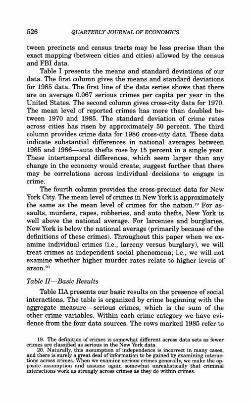
tween precincts and census tracts may be less precise than the exact mapping (between cities and cities) allowed by the census and FBI data.

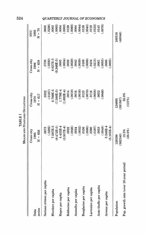
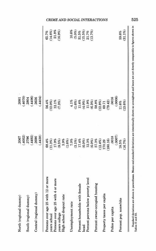
Table I presents the means and standard deviations of our data. The first column gives the means and standard deviations for 1985 data. The first line of the data series shows that there are on average 0.067 serious crimes per capita per year in the United States. The second column gives cross-city data for 1970. The mean level of reported crimes has more than doubled between 1970 and 1985. The standard deviation of crime rates across cities has risen by approximately 50 percent. The third column provides crime data for 1986 cross-city data. These data indicate substantial differences in national averages between 1985 and 1986-auto thefts rose by 15 percent in a single year. These intertemporal differences, which seem larger than any change in the economy would create, suggest further that there may be correlations across individual decisions to engage in crime.

The fourth column provides the cross-precinct data for New York City. The mean level of crimes in New York is approximately the same as the mean level of crimes for the nation.19 For as- saults, murders, rapes, robberies, and auto thefts, New York is well above the national average. For larcenies and burglaries, New York is below the national average (primarily because of the definitions of these crimes). Throughout this paper when we examine individual crimes (i.e., larceny versus burglary), we will treat crimes as independent social phenomena; i.e., we will not examine whether higher murder rates relate to higher levels of arson.20

Table II-Basic Results Table IIA presents our basic results on the presence of social

interactions. The table is organized by crime beginning with the aggregate measure-serious crimes, which is the sum of the other crime variables. Within each crime category we have evidence from the four data sources. The rows marked 1985 refer to

19. The definition of crimes is somewhat different across data sets as fewer crimes are classified as serious in the New York data.

20. Naturally, this assumption of independence is incorrect in many cases, and there is surely a great deal of information to be gained by examining interactions across crimes. When we examine serious crimes generally, we make the op- posite assumption and assume again somewhat unrealistically that criminal interactions work as strongly across crimes as they do within crimes.

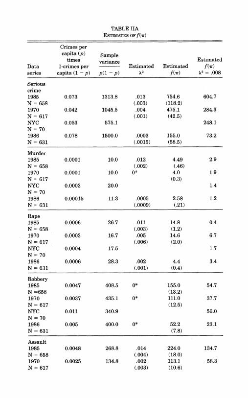
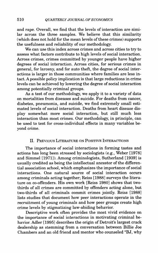
TABLE IIA ESTIMATES OF f(7r)

Crimes per capita (p) Sample

times variance Estimated Data 1-crimes per Estimated Estimated f(r) series capita (1 - p) p(l - p) X2 f(w) 2= .008

Serious crime 1985 0.073 1313.8 .013 754.6 604.7 N = 658 (.003) (118.2) 1970 0.042 1045.5 .004 475.1 284.3 N = 617 (.001) (42.5) NYC 0.053 575.1 248.1 N = 70 1986 0.078 1500.0 .0003 155.0 73.2 N = 631 (.0015) (58.5)

Murder 1985 0.0001 10.0 .012 4.49 2.9 N = 658 (.002) (.46) 1970 0.0001 10.0 0* 4.0 1.9 N = 617 (0.3) NYC 0.0003 20.0 1.4 N = 70 1986 0.00015 11.3 .0005 2.58 1.2 N = 631 (.0009) (.21)

Rape 1985 0.0006 26.7 .011 14.8 0.4 N = 658 (.003) (1.2) 1970 0.0003 16.7 .005 14.6 6.7 N = 617 (.006) (2.0) NYC 0.0004 17.5 1.7 N = 70 1986 0.0006 28.3 .002 4.4 3.4 N = 631 (.001) (0.4)

Robbery 1985 0.0047 408.5 0* 155.0 54.7 N =658 (13.2) 1970 0.0037 435.1 0* 111.0 37.7 N = 617 (12.5) NYC 0.011 340.9 56.0 N = 70 1986 0.005 400.0 0* 52.2 23.1 N = 631 (7.8)

Assault 1985 0.0048 268.8 .014 224.0 134.7 N = 658 (.004) (18.0) 1970 0.0025 134.8 .002 113.1 58.3 N = 617 (.003) (10.6)

TABLE IIA (CONTINUED)

Crimes per Sample capita (p) variance

times Estimated Data 1-crimes per Estimated Estimated f(ir) series capita (1 - p) p(1 - p) \2 f(7r) X2 = .008

NYC 0.0054 281.5 16.4 N = 70 1986 0.0056 296.4 0* 58.3 45.4 N = 631 (12.1)

Burglary 1985 0.019 424.1 .027 236 209.4 N = 658 (.003) (30) 1970 0.016 453.1 .009 257 173.4 N = 617 (.002) (26) NYC 0.013 112.3 53.4 N = 70 1986 0.02 480.5 .0011 63.9 30.7 N = 631 (.0007) (6.5)

Larceny 1985 0.04 743.8 .024 441 414.7 N = 658 (.005) (67) 1970 0.012 294.2 .005 186.4 170.5 N = 617 (.002) (18.2) NYC 0.01 1123.0 332.0 N = 70 1986 0.042 906.0 .0005 143.3 143.7 N = 631 (.0065) (100.5)

Auto theft 1985 0.008 651.3 .024 382.2 219.3 N = 658 (.004) (42.7) 1970 0.008 453.8 0* 340.3 140.8 N = 617 (31.1) NYC 0.015 356.7 88.0 N = 70 1986 0.009 648.9 .001 118.0 70.8 N = 631 (.0009) (10.2)

Arson 1985 0.00074 45.9 0* 33.1 22.2 N = 628 (3.6) 1986 0.00077 45.5 .0001 11.7 7.0 N = 578 (.0009) (.8)

The second column gives the ratio of the sample variance to the first column. Sample variance for cross- city data is defined below. (An analogous formula is used for cross-precinct variance):

I # cities Sample variance = t [(crime rate cityi - crime rate in US)*3popj2. # cities 2 w h

*X2 fixed at zero in cases where estimated X2 would have been negative.


the FBI cross-city data in 1985. The rows marked 1970 refer to the same FBI cross-city data but for 1970. The rows marked NYC refer to 1993 data for New York City precincts. While the number of locations is much smaller for NYC precincts (70 instead of 688), the average population of the precincts is roughly equivalent to the average population of cities in the cross-city sample. In Table IIA the sample size for 1985 cross-city data and NYC data do not change across columns. The sample size for 1970 cross-city data drops to a smaller sample of 617 cities because of data availabil- ity (for murder, rape, and larceny data).

The first column gives the average U. S. crime rate times one minus the average crime rate for each row. This number is the variance of cross-location crime rates (times the square root of population) that would be expected if criminal decisions were independent and if the expected proportion of criminals was constant across cities. This number provides us with a benchmark of predicted variance of cross-city crime rates weighted by the square root of city population.

Since we are estimating the variance across cities from a finite sample of cities, we are not surprised when the observed variance differs from the predicted variance. To gain confidence intervals around the predicted variance, we can use the fact that a sum of squared, standardized normal random variables follows a chi-squared distribution. Using this fact, and a standard chi- squared distribution table, we know that the observed variance of 70 independent units will lie between 0.61 and 1.49 times the true variance (p(l - p)) 99 percent of the time. Higher group sizes yield smaller confidence intervals. So an observed variance more than 1.5 times the predicted variance allows us to reject the null hypothesis. Since the observed variance is often over 1000 times the predicted variance and rarely less than twice the predicted variance, we will refrain from further discussion of statistical significance throughout the bulk of the remaining results.

The second column of Table IIA gives us the actual variance of crime rates (times the square root of city population) across locations divided by the first column. This number should, under the null hypothesis of independent crime decisions and constant expected crime levels across space be equal to one, which it is not. This figure is also a naive estimate of ftrr) which assumes that there is no relevant urban heterogeneity.

Columns three, four, and five show the results of first using preliminary regressions and working with the residuals of those


regressions. The crime rates have been orthogonalized with respect to the urban characteristics described in Appendix 2. The urban (city-specific) characteristics controlled for include (i) city population, (ii) regional dummies for location within the United States (North, South, Central, West), (iii) percent of persons over age 25 with 12 or more years of school, (iv) percent of persons over age 25 with 4 or more years of college, (v) unemployment rate, (vi) percent of households with a female head, (vii) percent of persons below the poverty level, (viii) percent of housing that is owner occupied, (ix) property taxes per capita, (x) police per capita, and (xi) percent of the population that is nonwhite. Crime rates are fitted to a logit curve, in which the crime rate is the left- hand side variable and the city-specific characteristics plus an intercept are treated as right-hand side variables.21 The pseudo R2's from these regressions are typically between 25 and 30 percent. The residuals from this procedure are then used to examine the variance of crime rates across space. The endogeneity of many of these variables with respect to crime should mean that we have overcorrected for city characteristics and that the variance in the fourth column of Table IIA may be an underestimate of the true variance.22

We also include a row for 1986 cross-city data. For these data we have included the 1985 crime rate of the same city as an explanatory variable. Our view is that including this lagged crime rate, which should eliminate almost all omitted urban character-

21. A logit curve is used rather than OLS because the crime rates are taken as probabilities (the probability of an agent committing a crime) and hence are bounded between zero and one. GMM is used to fit crime rates to the logit curve. We estimate these curves by minimizing the square of the residuals between the predicted crime rates and the actual crime rates. This procedure differs from standard logit curve estimation, which usually minimizes an error term in the expo- nentials. The advantage of our estimation procedure is that we are seeking a lower bound on the heterogeneity of unexplained crime rates, and our procedure minimizes that amount of unexplained heterogeneity. We tried various functional forms (including linear ones) for this "first-stage" procedure and found that our ultimate (second-stage) results are not sensitive to the functional form used. Nor are the second-stage results sensitive to the inclusion of various other city-specific characteristics, such as median age, proportion of young persons, percentage male, temperature variables, income per capita, growth in income per capita, number of migrants, percent owner-occupied houses, spending on governmental assistance programs, government expenditures generally, median house value, temperature variables, and many others.

22. Whenever crime influences a variable that we included as an explanatory variable, that variable will display explanatory power and will lessen the variance of the residual crime rate. However, the endogenous variable may not actually reflect an underlying difference in urban propensities to crime, rather it reflects the outcome of criminal choices. Including the endogenous variables causes the residual variance to be too low and the predicted variance to be too high.


istics except for those that change year to year, is a check on the presence of social interactions. Our model is about the choice to become a criminal, and many of those choices probably do not change from year to year. Controlling for last year's information about who chooses to become a criminal should lead us to underestimate the true cross-city variance to be explained by local interactions.

In columns three and four we show the results from jointly estimating X and f(t~) using standard GMM to estimate equation (16). Our estimation of the A parameter is meant to account for the possibility of omitted city characteristics. Our identification of X hinges on our model's prediction that (1) the variance of p* - p is independent of population so when this variance is weighted by the square root of population, the variance rises with population, while (2) the variance of (p - p*)CN should be independent of population. In Section III our model predicted that the difference between realized crime and predicted crime, conditioning on both observables and unobservables, should be constant when weighted by the square root of city size. In Section IV we assumed that the variance of p* - i, the distance between the predicted crime rate based on all variables and the predicted crime rate based on observables, was independent of city size.

We are now using these two facts, and the relationship in the data between (p - p)CN and CN (both of which we observe) to estimate the relative magnitudes of ftrr) (which comes from the size of (p - p*)CN) and X (which comes from the size of p* - '). We cannot estimate this for New York City data, because precincts have been designed so that each one has a population of approximately 100,000. Without variation in population size, it is impossible to estimate X.

If A is a function of N, this procedure is no longer valid. We checked for the possibility that A is a function of N by using the X's associated with the predicted values, and hoping that the variances of these X's, which are ultimately based on observable characteristics, would give us a guide to the variances of X's based on unobservables. Our procedure begins by setting p* equal to the predicted level of crime based on observables and setting p equal to national mean level of crime. As we then know p* - pf, we can use the fact that var(pj* -_ A) = T(X ,A)pj2(1 -^ )2, to estimate X. We estimated separate A values for ten equally sized groups of cities sorted by population and found that these X values do not change with population size within the first eight groups. The


two highest population groups of cities had somewhat lower X values. Since this deviation from our assumption for the highest population cities was troubling, we then reestimated our f(ir)'s for the smallest 80 percent of our cities and found results similar to those in Table IIA.23

The estimates of X2 in Table HA range from zero to 0.027. These estimates support the premise that the variance is not ultimately accounted for by differences in city characteristics. The estimated ftr)s are in the fourth column, and many of the quali- tative results of earlier sections are essentially unchanged. We also have standard errors bounding the f(wr) estimates so we can again note that almost all of these estimates are statistically different from one. Serious crimes, burglary, larceny, assault, and auto theft all display large amounts of social interaction. Rape, murder, and arson display much lower levels of social interaction.

The fifth column shows the value of f(rr) when we orthogo- nalize with respect to urban characteristics and then assume a fixed value for X2, .008. This number was chosen by determining how much explanatory power controlling for lagged crime rates had in the 1986 serious crime explanatory regressions. This value was chosen as a multiple of the explanatory power created by controlling for lagged crime rates in the 1986 serious crime regressions.

We transformed this explanatory power into an estimate for X by first assuming that the lagged 1985 serious crime rate was the only missing variable in the 1986 serious crime regressions. By comparing the p*'s which are found by controlling for the lagged crime rate and the i's which are found by controlling for all variables except for the lagged crime rate, we find a value for p* - k and, since var(pj* - p ) = P(X1j5) j2 (1 - p )2we found a benchmark value for X2 of 0.004. We then assumed that the remaining observables (for all the equations) had twice as much explanatory power as the lagged crime rate; i.e., we doubled this benchmark value of X2 to 0.008.24 Of course, doubling the value of X2 is fairly arbitrary, and reasonable estimates of unobserved heterogeneity could be far from this number. While perturbations in the size of X2 do certainly change the estimates of f(wr), in the

23. The f( r) estimates for the smaller city sample remained both statistically and economically far from one for all crimes except rape and murder. This procedure follows a suggestion from Kevin Murphy.

24. This assumption is similar to assumptions used by Murphy and Topel [1990], who use the distributions of observable attributes to form benchmark estimates of the distributions of unobservable attributes.


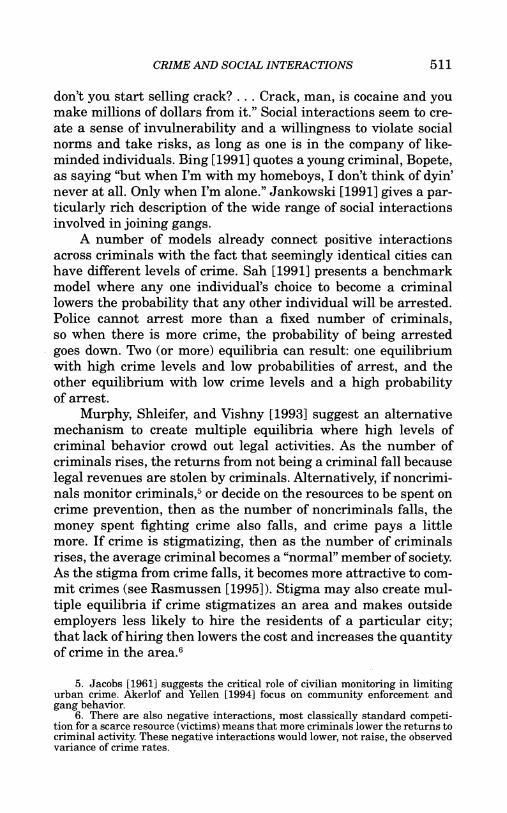
800 Serious Crimes

700/

600/

f(On) estimated / from 1985 cross- 500 city data, 400 Auto Theft Larceny lambda- squared=.008, 300 Robbery from Table IIA. 200 Assau X Burglary

100 Ason

0 Murder, Rape

0 50 1600 1 50 200 250 300 350 400 450 500 550 600 650 700

f(i) estimated from cross-city 1985 data, lambda-squared is estimated, from Table IIA. y = 1.155x - 36.12, R-squared: .953

(.097)

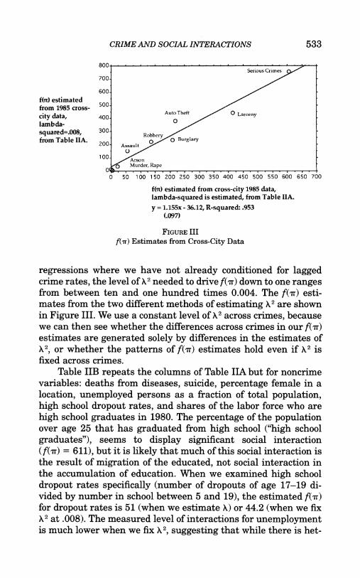
FIGURE III fur) Estimates from Cross-City Data

regressions where we have not already conditioned for lagged crime rates, the level of X2 needed to drive f(r) down to one ranges from between ten and one hundred times 0.004. The f(rr) estimates from the two different methods of estimating X2 are shown in Figure III. We use a constant level of X2 across crimes, because we can then see whether the differences across crimes in our f( r) estimates are generated solely by differences in the estimates of X2, or whether the patterns of ftrr) estimates hold even if X2 is fixed across crimes.

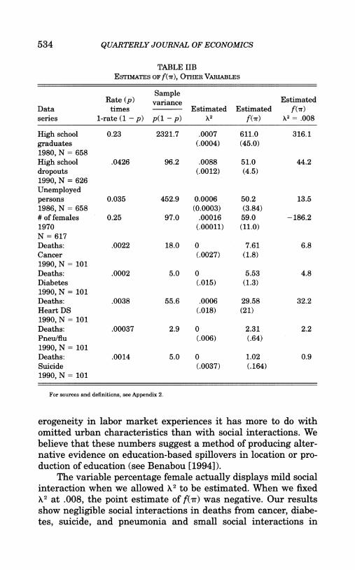
Table IIB repeats the columns of Table IIA but for noncrime variables: deaths from diseases, suicide, percentage female in a location, unemployed persons as a fraction of total population, high school dropout rates, and shares of the labor force who are high school graduates in 1980. The percentage of the population over age 25 that has graduated from high school ("high school graduates"), seems to display significant social interaction (f(rr) = 611), but it is likely that much of this social interaction is the result of migration of the educated, not social interaction in the accumulation of education. When we examined high school dropout rates specifically (number of dropouts of age 17-19 divided by number in school between 5 and 19), the estimated f( r) for dropout rates is 51 (when we estimate X) or 44.2 (when we fix X2 at .008). The measured level of interactions for unemployment is much lower when we fix X2, suggesting that while there is het-


TABLE IIB ESTIMATES OF f(ir), OTHER VARIABLES

Sample Rate (p) variance Estimated

Data times Estimated Estimated f(ir) series 1-rate (1 - p) p(l - p) X2 f(Q') X2 = .008

High school 0.23 2321.7 .0007 611.0 316.1 graduates (.0004) (45.0) 1980, N = 658 High school .0426 96.2 .0088 51.0 44.2 dropouts (.0012) (4.5) 1990, N = 626 Unemployed persons 0.035 452.9 0.0006 50.2 13.5 1986, N = 658 (0.0003) (3.84) # of females 0.25 97.0 .00016 59.0 -186.2 1970 (.00011) (11.0) N = 617 Deaths: .0022 18.0 0 7.61 6.8 Cancer (.0027) (1.8) 1990, N = 101 Deaths: .0002 5.0 0 5.53 4.8 Diabetes (.015) (1.3) 1990, N = 101 Deaths: .0038 55.6 .0006 29.58 32.2 Heart DS (.018) (21) 1990, N = 101 Deaths: .00037 2.9 0 2.31 2.2 Pneu/flu (.006) (.64) 1990, N = 101 Deaths: .0014 5.0 0 1.02 0.9 Suicide (.0037) (.164) 1990, N = 101

For sources and definitions, see Appendix 2.

erogeneity in labor market experiences it has more to do with omitted urban characteristics than with social interactions. We believe that these numbers suggest a method of producing alternative evidence on education-based spillovers in location or pro- duction of education (see Benabou [1994]).

The variable percentage female actually displays mild social interaction when we allowed X2 to be estimated. When we fixed X2 at .008, the point estimate of f(Ir) was negative. Our results show negligible social interactions in deaths from cancer, diabetes, suicide, and pneumonia and small social interactions in


deaths from heart disease in a sample of 101 cities. We find these results comforting as they suggest that our methodology does not find social interaction in the percent female or in diseases that are to a large extent inherited. Any remaining interactions are probably the result of migration decisions of high-risk popula- tions and migration of women.

Table III-Repeat Offenders

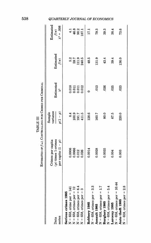
One of the simplifications in Table IIA is that we assume that each crime is perpetrated by a different individual and reflects an agent's decision to enter a life of crime (at least for that year). Agents frequently commit more than one crime within a given year. These repeat crimes provide a degree of correlation across crimes, because if an agent commits one crime, we expect that he will commit more crimes. This effect would reveal itself as a social interaction in Table IIA, which does not actually require any cross-individual interactions. If we actually had data on criminals rather than crimes, this problem would disappear, but since crime data are the only data available, it is necessary that we deflate our measures to allow for the possibility that when some- one is seen committing one crime, it is more likely that the individual will commit more crimes.

More complicated and realistic models of multicrime criminals are beyond the scope of this paper, but we can make a simple correction and assume that if there are pj crimes in a city then the city has pjlR criminals, where R refers to the number of repeat offenses per criminal. In our estimation procedure we simply replaced the crime rate with the crime rate divided by R for each city. This correction uniformly lowers the estimated f(Tw)'s in our sample. The intuition for this can be gained by thinking about our estimate of f(Tw) when cities are homogeneous (predicted crime rates are constant and X = 0). In that case, our estimate of f(Tr) is var(pj)/(p(l - p)), where p = E(pj). When we replace the observed crime rate with the observed crime rate divided by R, our new estimator of f(IT), which we label f(IT)R is var(pj/R)/ I(p/R)(1 - (pIR))]. Simple algebra shows that

(22) f( ) var(pj) R2 var(pj/R) R var(pj/R) p(l - p) p(l - p) (p/R)(1 - p)

R var(pj/R) (p/R)(1 - (pIR)) = Rf(IT)R.


When we correct for multiple crimes per criminal, the estimated f(wl) decreases in magnitude by roughly the number of crimes per criminal (R).

Our estimates for the number of crimes per criminal come from various sources. For serious crimes we took the value of 6.4 crimes per criminal from a self-reported measure in the Rand Prison Inmate Survey [Chaiken 1978]. This number, undoubt- edly, is biased upward since repeat criminals are more likely to be incarcerated.25 For serious crimes we also estimated f(A )'s assuming 3 crimes per criminal and 141 crimes per criminal, to find a range of possible estimates for f(ir). For individual crimes we used Blumstein and Cohen's [1979] study of arrest records. These data may underestimate repeat offenses since only crimes where arrests were made are counted in the study. There may also be overestimates since only arrested criminals are included in the study (and arrested criminals are more likely to be repeat offenders).

The overall effect of these controls is to lower the estimated ftir)'s. Most of the ftir)'s remain above 38 which indicates a great deal of social interaction. Only when we use 141 crimes per year (which comes from self-reported DiIulio and Piehl [1991] numbers), do social interactions completely disappear. Since those numbers include both serious and nonserious crimes and because they rely on self-reported figures that seem (to us at least) highly implausible, we do not find these observations to present serious questions about our results.

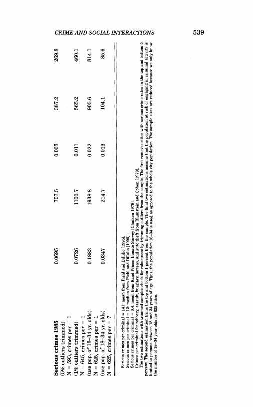
The third section of Table III contains two more checks for robustness. We tried trimming outliers from the sample by re- moving those cities with the highest and lowest reported crime rates. Naturally, this reduces the observed variance of crime rates and hence ftrr). However, even after trimming the upper and lower 5 percent from the sample, we still find an ftir) of 387.2 for serious crimes. When we trim only the top and bottom 1 percent, we estimate f(wr) at 565.2 (down from 754.6 when we use the entire sample).

The last two lines in Table III alter the assumption about the population at risk of performing criminal activities. Instead of using the entire city population to calculate crime rates and f(rr), we use only persons 18-34. This new assumption does not lower our point estimates of f(ir). For example, if we assume one crime

25. Although it is possible that the extreme repeat offenders avoid incarcera- tion completely.


per criminal and limit the population to persons 18-34 we find an ftwr) of 905.6 in contrast to 754.6 when the whole city population is used.

Interpreting f(,r)

While f(rr) can simply be interpreted on its own as an index of social interaction, we find it useful to discuss 17r, which is the expected distance between two fixed agents; following the model, 1/'rr = (1 + f(rr))/2. This distance is the expected size of an unbro- ken line of interconnected agents, or the expected size of a "clique" of interacting agents. Viewed in this way, our empirical results can be seen as asking "how big must social groupings be to justify the observed cross-city variance?"

In Table IIA the values for f(i) tell us that the average clique size for serious crimes in general ranges from 657 (for uncon- trolled data) to 37 (for data that has been controlled for city characteristics, lagged crime rates and then additionally allowed for unobservables to be twice as important as that lagged crime rate).26 Our best estimate of the clique size (which includes controlling for urban characteristics and estimating X) is 377. The comparable estimates of clique size for larceny and auto theft are 221 and 191, respectively. Our best estimates of average clique sizes for robbery, burglary, and assault are 78, 118, and 112, respectively. Our best estimate of the average clique size for murder is two, and for rape the average clique size is seven.

The high values of ftrr) for serious crimes, relative to many other crimes, is explained by two distinct forces. First, the bulk of serious crimes are larcenies, and f(ir) values for larceny are high. Second, the observed f(rr) for serious crimes is a function both of (1) the interactions within crimes and (2) the interaction across individual crimes (i.e., the fact that more murders de- crease the costs of robbery). Since the f(ta) for serious crimes includes both of these effects, while the f(ir)'s for individual crimes include only within-crime interactions, we would expect the f(rr) for serious crimes generally to be higher than a weighted average of the f(ir)'s estimated for the individual crimes. While we are not seriously examining the interaction across crimes here, this high level of f(ir) suggests that there is a significant quantity of in- tercrime spillovers.

26. Since the serious crimes estimate assumes perfect cross-crime interactions and the other estimates assume no cross-crime interactions, the results are noncomparable.


*5,< 1loooo ~ > cs c t7- C 1t- pi c o0.. o

4WiI m

U l

tt- co C tn - w q

X ? : - t m LO LO C ) O C:v .> O

2go~~~~~~~~~~~~~~~~( Vcd

UID .CX co o co o

i Q g; o o o o oo ob o

z N r-4 -4C9 Co C0 LO CO 0 0 0 C) 0 0 0

6666 .E...X.?

00

o6 r4r4 6 0 t-~ 0 -X oo b oo1 co o0 C.0 cq

~z

w C) - C-4 0 0

o 0 0 01 '-4) CU1 Co C) Co

, QC 0 -C 0 0 0 0 0

0000 0 0 00 0- H ~~~ 6666 6 6~~~~~ 0 0) 0

06 6 0-4- 0 . 60 0 to t U5Co Co U5 lo to 4 c

'-4 hO 1111 I I I I r: zzII09z zmz 5


00 ~ ~ eD 0 03

0W C' 00 o0

00~ ~~0

tw r. u

cq C.0 Q)~~~~* a)

6~~~~~~~~~n o6 0'

00 VQ 0s 0sdd

o D

,m :O

(M cq 00 ~ ~ ~ -0

00 t4 00 M r. 0

o 0 0 0 33 | i @&3v

~0

00

ko o 00 oo $0 00 '-

00

CJ u0 u~~~ o~0~*

P. 0 , 0 4

63 6 63 6 4h?

a S z X t o >o N o o: W oM W

CoL.)

n o e~~~~~~~ o 0 'UA1 mtCOQ

t :Z z z

;=ZQSs

z 0+0-.


Extensions27

As mentioned previously, the observed social interactions could be measuring both local influences on choices about crime and criminals' moving into the same area. Adult criminals will have had more time to migrate and are more likely to have chosen the location they are inhabiting. Young agents (particularly those eighteen and under) have little ability to choose their location. If the observed social interactions are the result of criminals' migrating, then we would expect the crimes committed by older criminals to display higher rates of social interactions.

If we regress the f rr) estimates from Table IIA on the percentage of individuals arrested for each crime who are eighteen and under, the correlation between social interaction and youth- fulness is weakly positive.28 If we eliminate arson, the correlation coefficient between these two variables rises to over 70 percent. While we have only eight observations and other factors could easily be driving this correlation, the results suggest that the interactions we observe are more likely to be the result of local influence and not the result of migrational clustering of criminals. The results also corroborate the other evidence that young people are more influencable by their peers, e.g., Reiss [1988] shows that younger criminals are more likely to act in groups.

So far, we have assumed that ftrr) is invariant across cities. In fact, there are many reasons why we might believe the level of interactions changes across cities. Urban characteristics drive the mean level of crime rates, but they also may determine the extent to which agents interact and the extent to which patterns of crime move across the city unit. We have also performed estimations where both X and f(wr) are estimated in a cross-city regression. We allowed three city characteristics (level of education, percent nonwhite and percent female-headed household) to influence our estimate of f(wr).

Our basic regression connecting ftrr) with city level characteristics for 1985 found that race basically failed to influence the level of interactions except for murder and larceny, where bigger racial minorities created lower levels of interactions. The level of education lowered the degree of interaction for murder and robbery, but raised the degree of interaction for larceny. The percent

27. These extensions are discussed more thoroughly in the working paper version of this paper [Glaeser, Sacerdote, and Scheinkman 1995].

28. The results are unchanged if we look at the share of arrestees who are 24 and under.


of female-headed households raised the levels of social interaction for murder, serious crimes generally, burglary (at the 10 percent level), and larceny. The female-headed household variable had the expected sign and suggests that parental influence provides an alternative information source to peer effects.29

The Form of the Interaction

This work only suggests the relevance of a social interaction, not the form of that interaction or the mechanisms that aid that interaction. Space constraints prohibit a serious attempt to isolate the exact form of the interaction, but we can present some suggestive facts here. A candidate interaction mechanism should be measurable by a variable that is strongly positively correlated with crime so that controlling for that variable eliminates much of the variance of crime rates, and furthermore this correlation must represent two-sided causality (shown with instrumental variables techniques for example).

These criteria immediately rule out any mechanism that op- erates through congestion in law enforcement. There is no correlation between arrest rates (arrests per crime) and crime across NYC precincts.30 Across cities in 1985 the correlation between arrest rates and crime rates is -0.08 which means that arrest rates can explain less than 1 percent of the observed variation in crime rates.3' We must conclude that high crime creating lower arrest rates plays only a marginal role in explaining cross-city crime variance.32

Likewise, if we consider the possibility that high crime rates reduce the returns to education which in turn increase crime, the data would again reject this potential interaction mechanism. The partial correlation between education and crime that condi-

29. The idea that peer influence is a substitute for parental influence is sup- ported also by descriptive work. Bing [1991] quotes another young criminal, Side- winder, as saying "That's [the gang] the only thing I'm connected to, that's my family."

30. Perhaps this fact occurs because police concentrate their resources more in high crime rate areas. If communities with higher crime rates hire more police officers and end up having higher arrest rates (as a positive correlation between crime and arrest rates indicates), it means that there is a negative interaction term across individuals (which would eliminate cross-city variance completely, not exacerbate that variance).

31. The strongest correlation between arrest rates and crime rates is in 1970, but this correlation is only -0.18 which still means that arrests are explaining less than 4 percent of crimes. Controlling for population, population growth, four regional dummies, and percent nonwhite greatly reduces the explanatory power of the 1970 data.

32. There is also no correlation (less than 0.05) between the likelihood of being convicted and rates of crime.


tions just on demographics (city population, population growth, and percent nonwhite) and regional dummies is -0.05 in 1985. Likewise, the partial correlation between unemployment and crime is less than 0.10 in 1985. Finally, the correlation between female-headed households and serious crimes is 0.59 in 1970, 0.42 in 1985, and 0.22 across NYC precincts. The corresponding conditional correlation coefficients are 0.33 in 1970, 0.32 in 1985, and -0.10 across NYC precincts. These preliminary results suggest it seems more likely that interaction mechanisms will rely on family instability, not unemployment or schooling or low arrest rates.

VI. CONCLUSION

This paper has reexamined the extreme cross-city and cross- precinct crime variance and found that either unobserved heterogeneity is much higher than observed heterogeneity or criminals' decisions in a metropolis are highly dependent. Our two models of social interactions provide a framework for understanding the observed variance of cross-city crime rates. More importantly, these models provide us with a natural index of social interactions: the proportion of potential criminals who do not respond to social influences.

We used this index to measure the importance of social interactions to criminal behavior in the United States across cities and across precincts in New York. Even allowing for a wide diversity in underlying characteristics across cities (even more than is shown by observable characteristics), we found a large amount of social interaction in criminal behavior. The cross-city variance is quite high to be rationalized as the outcome of independent decisions to engage in crime-we believe that the evidence suggests covariance across agents.

Our index showed that there is a wide range in the degree of interactions across crimes, but that across data samples, the rough level of interactions stayed constant for each crime. The estimates for average social group size ranged from. one to five for murder. Similarly low levels of social group size were found for rape and arson. The average social group sizes for auto theft and larceny were over 200 in most of our estimations. For robbery, assault, and burglary, estimated clique sizes were approximately 100.


Across crimes we found that crimes committed by younger criminals have more social interactions. Across cities we found higher levels of social interactions (for serious crimes generally, for petty larceny, and for auto theft) in cities with more female- headed households. While these results are preliminary, we inter- pret them to mean that the average social interactions among criminals are higher when there are not intact family units. The presence of strong families interferes with the transmission of criminal choices across individuals.

APPENDIX 1: MODEL WITH SYMMETRIC IMITATION

In this appendix we present an alternative to the model of social interactions that we discussed in the text. Its main advantage is that it allows for symmetric imitation; individuals simultaneously imitate and are imitated by other individuals. The disadvantage is that we do not explicitly model the optimization problem. We simply assume that each individual chooses the action that is currently being adopted by a random neighbor. The model we present is a variation of the "voter model" in the physical sciences (e.g., Kinderman and Snell [1980]).

We assume that each agent is indexed by an integer i, and that each agent can choose one of two actions {0,1}. Action 1 will be interpreted as committing a crime. Although a dynamic model will be presented, we are only interested in the properties of its stationary distribution.

At time 0 each agent chooses an action a? independently and the probability that an agent chooses action 1 is p. The neighbors of an agent i are the agents in N(i) = {i - 1,i + 1}. With probability IT > 0 and with independence across agents, an agent i belongs to a set S. Associated with each agent i e S, there is an independent Poisson process with mean time 1. At each epoch of the Pois- son process associated with i, the action of agent i changes to that of one of its neighbors with equal probability. Note that agents in S are "stuck," while agents not in S imitate their neighbors.

This defines stochastic processes at, the action at t of agent i for each integer i. The reader familiar with the literature on voter models will recognize that except for the presence of some agents who are stuck at their initial action, i.e., those i E S, this is exactly a one-dimensional voter model. This difference, however, is important since one-dimensional voter models have stationary


distributions that exhibit unanimity, i.e., all agents (in the limit) choose the same action.33

For given parameters (prar) we argue that there is an invariant limit measure [u(p,r). More precisely, given any n, there exists a limit measure Fin(Pr) defined over configurations of Jai: lit < n}, and if m > n, the measure induced over the configurations of {ai: lil < n} by p..(pyr) agrees with Sl(Pyr)-

To see this, first consider the measure [u(pw) given the set S and the a? for each i E S. Given any integer i M S, we write i for the largest element of S which is less than i, and i+ for the smallest element of S which is greater than i. In other words, i_ and i+ are the elements of S that "bracket" i. If a0 = a? , then as t -? oo, it is easy to see that a' -* a? with probability one. Hence ,u(py) assigns probability one to the set of configurations in which a. is constant for i_ c j c i+. If a? =# a? , then it is again easy to see that with probability approaching one as t -- oo if at = a0 then for any i_ j c< i, a' = a? , i.e, the agents' states are "sorted." Hence, conditional on S and the a? for each i GE S, p(p,r) assigns probability one to the set of configurations that are sorted in this way. Furthermore, if a?? = a? , each of the possible A = 1 + i+ - i sorted states has the asymptotic probability of 1/A. The measure pu(p,w) can now be constructed by considering the independent distributions over possible sets S and initial a? for each i E S. Obviously, E(ai) = p, where the expected value is taken over the invariant measure jL(py). Also the sequence fail is stationary; i.e., the joint distribution of any finite set of a's is unchanged by shifting all i's by a fixed integer.

We now consider the normalized sum 1/ 2n + 1lii5n

(ai - p), where the ai are distributed according to the invariant measure. Just as in our model in the text, the presence of fixed agents guarantees central limit behavior for the normalized sum. The computation of the asymptotic variance r2 is lengthier (available upon request), but one can show that

a 2 = ?(,U)p( - p),

33. This unanimity result implies too much variation in crime rates relative to the data. In fact, per capita rates would be zero or one. Unanimity also prevails in two-dimensional voter models; i.e., where each agent is indexed by a pair (i, j) and a neighbor is any agent (i, j ? 1) or (i ? 1, j). In dimension three, unanimity disappears and under any invariant distribution the number of agents that choose action 1 on a cube of total population n, converges to a normal random variable when divided by n516, as opposed to the usual Cn (cf. Bransom and Griffeath [1979]). We found that this alternative scaling also predicts a higher variance than that found in the data.


where A(1) = 1, f'(1) < 0 and limlr<f(i) = oo. Hence the qualita- tive behavior of the variance matrix is exactly as in the model in the text.

APPENDIx 2: VARIABLE DEFINITIONS

Definition Source

Serious Crime The sum of Part 1 offenses FBI Uniform Crime defined under the FBI's Reports in Crime in the Uniform Crime Reporting United States 1970, 1985, program. Part I offenses 1986; New York City include murder, rape, Police Data in Statistical robbery, assault, burglary, Report: Complaints and larceny, and auto theft. Arrests 1993 The New York City (NYC) precinct data exclude those Part I crimes that are not felonies, for example larcenies < $1000. Hence NYC data are not fully comparable to cross-city data. All NYC precinct data are for 1993.

Murder UCR definition: The willful FBI Uniform Crime and nonnegligent killing of Reports; NYC Police Data one human being by (see above and references) another. Excludes manslaughter by negligence and traffic fatalities.

Rape The carnal knowledge of a FBI Uniform Crime female forcibly and against Reports; NYC Police Data her will. Excludes statutory rape.

Robbery The taking or attempt to FBI Uniform Crime take anything of value Reports; NYC Police Data from the care, custody, or control of a person by force or threat of force.

Assault An unlawful attack by one FBI Uniform Crime person upon another for Reports; NYC Police Data the purpose of inflicting severe or aggravated bodily injury.

Burglary The unlawful entry of a FBI Uniform Crime structure to commit a Reports; NYC Police Data felony or a theft.


APPENDIX 2: (CONTINUED)

Definition Source

Larceny The unlawful taking, carrying, leading, or riding away of the property of FBI Uniform Crime another. Reports; NYC Police Data

Auto theft The theft or attempted FBI Uniform Crime theft of a motor vehicle. Reports; NYC Police Data

Arson Any willful or malicious FBI Uniform Crime burning or attempt to Reports burn, with or without attempt to defraud, a dwelling house, public building, motor vehicle or aircraft, personal property of another.

Population, all City population as defined 1970 Census of samples by Bureau of the Census Population data; 1980

Census of Population data in County and City Data Book 1972, 1988

Regional dummies Uses regions (North, South, Central, West) as defined by Bureau of the Census

Persons over age 25 Census of Population data with 12 or more in County and City Data years school Book 1972, 1988 Persons over age 25 Census of Population data with 4 or more years in County and City Data college Book 1972, 1988 Unemployment rate Civilian labor force Bureau of Labor Statistics

unemployment rate. data in County and City Standard Labor Data Book 1972, 1988 Department definition

Percent households Female householder. No Bureau of the Census with female head spouse present. data in County and City

Data Book 1972, 1988 Percent persons Bureau of the Census below poverty level data in County and City

Data Book 1972, 1988 Percent owner- Owner-occupied housing Bureau of the Census occupied housing units/occupied housing data in County and City

units Data Book 1972, 1988 Property taxes per Total property taxes Bureau of the Census: capita collected during fiscal year/ County and City Data

population Book 1972, 1988


APPENDIX 2: (CONTINUED)

Definition Source

Police per capita Full-time city law FBI data in County and enforcement officers/ City Data Book 1972, population 1988

Percent population Bureau of the Census nonwhite data in County and City

Data Book 1972, 1988 High school dropout (Persons 16-19 not Bureau of the Census rate enrolled in school and not data in County and City

high school graduate Data Book 1994 1990)/(above group + persons enrolled in elementary and high school 1990)

Death rates (cancer, Deaths attributed to cause Vital Statistics of the diabetes, etc.) in 1990/population United States, Volume 2

HARVARD UNIVERSITY AND NATIONAL BUREAU OF ECONOMIC RESEARCH

HARVARD UNIVERSITY UNIVERSITY OF CHICAGO

REFERENCES

Adler, W., Land of Opportunity: One Family's Quest for the American Dream in the Age of Crack (New York, NY: Atlantic Monthly Press, 1995).

Akerlof, G., and J. Yellen, "Gang Behavior, Law Enforcement and Community Values," in H. Aaron, T. Mann, and T. Taylor, eds., Values and Public Policy (Washington, DC: Brookings Institution, 1994).

Becker, G. S., "Crime and Punishment: An Economic Approach," Journal of Politi- cal Economy, LXXVI (1968), 169-217.

Benabou, R., "Education, Income Distribution and Growth: The Local Connec- tion," NBER Working Paper No. 4798, 1994.

Bing, L., Do or Die (New York, NY: Harper Collins, 1991). Blumstein, A., and J. Cohen, "Estimation of Individual Crime Rates from Arrest

Records," Journal of Criminal Law and Sociology, LXX (1979), 561-85. Bransom, M., and D. Griffeath, "Renormalizing the Three Dimensional Voter

Model," Annals of Probability, VII (1979), 418-32. Case, A., and L. Katz, "The Company You Keep: The Effect of Family and Neigh-

borhood on Disadvantaged Youth," NBER Working Paper No. 3705, 1991. Chaikin, J., "Rand Prison Inmate Survey," Rand Working Paper WN-10107-

DOJ, 1978. Crime in the United States: Federal Bureau of Investigation Uniform Crime Re-

ports (Washington, DC: U. S. Government Printing Office, 1970, 1985, 1986). County and City Data Book (Washington, DC: U. S. Government Printing Office,

1972, 1988, 1994). DiIulio, J., and A. Piehl, "Does Prison Pay," Brookings Review, IX (Fall 1991),

28-35. Ehrlich, I., "The Deterrent Effect of Capital Punishment: A Question of Life and

Death," American Economic Review, LXV (1975), 397-417.


Ellison, G., and E. Glaeser, "Geographic Concentration in Manufacturing Indus- tries: A Dartboard Approach," NBER Working Paper No. 4840, 1994.

Feller, W., An Introduction to Probability Theory and Its Applications (New York, NY: John Wiley, 1968).

Freeman, R., "Crime and the Employment of Disadvantaged Youths," NBER Working Paper No. 3875, 1991.

Glaeser, E., B. Sacerdote, and J. Scheinkman, "Crime and Social Interactions," NBER Working Paper No. 5026, 1995.

Hall, P., and C. C. Heide, Martingale Limit Theory and Its Applications (New York, NY: Academic Press, 1980).

Jacobs, J., The Death and Life of Great American Cities (New York, NY: Random House, 1961).

Jankowski, M., Islands in the Street: Gangs and American Urban Society (Berke- ley, CA: University of California Press, 1991).

Jovanovic, B., Aggregate Randomness in Large Noncooperative Games," mimeographed, 1985.

Kindermann, R., and J. L. Snell, "On the relationship between Markov Random Fields and Social Networks," Journal of Mathematical Sociology, VII (1980), 1-13.

Lane, R., Violent Death in the City: Suicide, Accident and Murder in Nineteenth Century Philadelphia (Cambridge, MA: Harvard University Press, 1979).

Levitt, S., "Reporting Behavior of Crime Victims and the Size of the Police Force: Implications for Studies of Police Effectiveness Using Reported Crime Data," mimeographed, 1994.

Murphy, K. M., A. Shleifer, and R. Vishny, "Why Is Rent Seeking So Costly to Growth?" American Economic Review, LXXIII (1993), 409-14.

Murphy, K. M., and R. Topel, "Efficiency Wages Reconsidered: Theory and Evi- dence," in Y. Weiss and G. Fishelson, eds., Advances in the Theory and Mea- surement of Unemployment (London, UK: Macmillan, 1990).

Quetelet, A., Sur l'Homme et le Developpement De Ses Facultes (Paris: Bachelier, 1835).

Rasmussen, E., "Stigma and Self-Fulfilling Expectations of Criminality," mimeographed, 1995.

Reiss, A. J., "Understanding Changes in Crime Rates," in S. Feinberg and A. J. Reiss, eds., Indicators of Crime and Criminal Justice: Quantitative Studies (Washington, DC: Bureau of Justice Statistics, 1980). , "Co-offending and Criminal Careers," in M. Tonry and N. Morris, eds., Crime and Justice: A Review of Research, Volume 10 (Chicago, IL: University of Chi- cago Press, 1988).

Sah, R., "Social Osmosis and Patterns of Crime," Journal of Political Economy, XCIX (1991), 1272-95.

Scheinkman, J. A., and M. Woodford, "Self-organized Criticality and Economic Fluctuations," American Economic Review, LXXXIV (1994), 417-21.

Simmel, G., George Simmel On Individuality and Social Forms (Chicago, IL: Uni- versity of Chicago Press, 1971).

Statistical Report: Complaints and Arrests, mimeographed, New York City Police Department, 1993.

Sutherland, E., Principles of Criminology, 3rd ed. (Philadelphia, PA: Lippincott, 1939).

Weber, M., Economy and Society, 2 Volumes (Berkeley, CA: University of Califor- nia Press, 1978).

Wilson, J. Q., and R. Herrnstein, Crime and Human Nature (New York, NY: Si- mon and Schuster, 1980).

Vital Statistics of the United States, Volume II, Section 6, Life Tables (Hyattsville, MD: United States Department of Health and Human Services, National Center for Health Statistics, 1990).

1990 Census Data By Police Precinct, mimeographed, New York City Department of City Planning, 1993.

Documents

Crime and Social Interactions - Princeton Universityjoses/pp/crime.pdf · CRIME AND SOCIAL INTERACTIONS* ... The media trumpet the large rise in crime since the 1960s, ... crime levels