Lindahl Lecture 2: Social Interactions, Crime, Ghettos and Hatred

Edward L. Glaeser

Harvard University

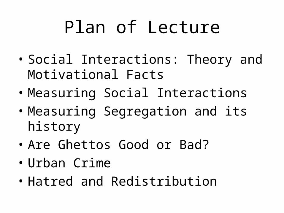
Plan of Lecture

• Social Interactions: Theory and Motivational Facts

• Measuring Social Interactions

• Measuring Segregation and its history

• Are Ghettos Good or Bad?

• Urban Crime

• Hatred and Redistribution

The Power of Social Interactions

• The Strong Form of the Social Interactions Hypothesis is that we are largely formed by the people around us

• Skills (Kain and Spatial Mismatch)

• Preferences

• Beliefs

• Other positive interactions (e.g. reducing probably of being caught)

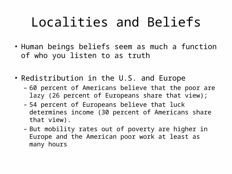
Localities and Beliefs

• Human beings beliefs seem as much a function of who you listen to as truth

• Redistribution in the U.S. and Europe– 60 percent of Americans believe that the poor are lazy

(26 percent of Europeans share that view); – 54 percent of Europeans believe that luck determines

income (30 percent of Americans share that view).– But mobility rates out of poverty are higher in Europe

and the American poor work at least as many hours

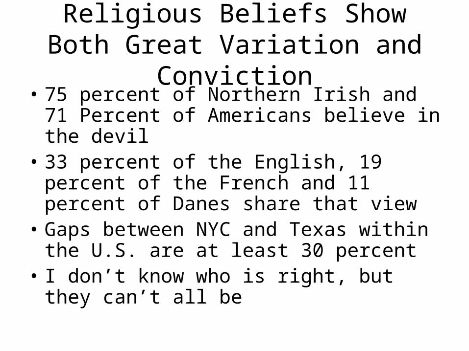
Religious Beliefs Show Both Great Variation and Conviction

• 75 percent of Northern Irish and 71 Percent of Americans believe in the devil

• 33 percent of the English, 19 percent of the French and 11 percent of Danes share that view

• Gaps between NYC and Texas within the U.S. are at least 30 percent

• I don’t know who is right, but they can’t all be

Approaches to Measuring Social Interactions

• Correlation with group averages

• Impact of Neighborhood more generally

• Group level heterogeneity, excess variance

• Social Multipliers

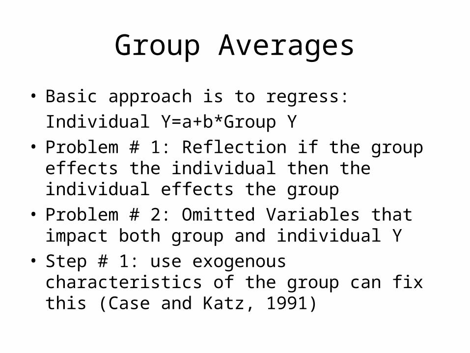
Group Averages

• Basic approach is to regress:

Individual Y=a+b*Group Y• Problem # 1: Reflection if the group effects the

individual then the individual effects the group• Problem # 2: Omitted Variables that impact both

group and individual Y• Step # 1: use exogenous characteristics of the

group can fix this (Case and Katz, 1991)

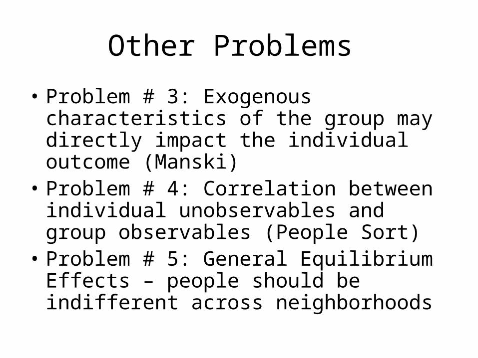
Other Problems

• Problem # 3: Exogenous characteristics of the group may directly impact the individual outcome (Manski)

• Problem # 4: Correlation between individual unobservables and group observables (People Sort)

• Problem # 5: General Equilibrium Effects – people should be indifferent across neighborhoods

The Rise of the Randomized Neighborhood

• Moving to Opportunity (Katz, Kling, Liebman, Ludwig)– Randomized Trial Voucher experiment– Confusing Income and Location– Effects are modest on kids

• Sacerdote (2003) QJE– randomized roommates – big social, small academic

• Aslund, Edin and Fredriksson (2003)– randomized immigrants– big effects

Excess Variance: Theory (QJE 96)

• Basic statistics tells us that the standard deviation of a set of averages should be p(1-p) divided by the square root of n

• But for many things, variances are much higher

• In the case of crime, variance is 1500 times crimes per capita*1-crimes per capita

Three Explanations for High Variance of Crime Rates

• Omitted Variables (policing, etc.)

• High crimes per criminal

• Social interactions– Congestion of law enforcement (but areas

spend more when there is more crime)– Legitimizing crime/preference formation– Transmitting Knowledge– Reducing returns to legal activities

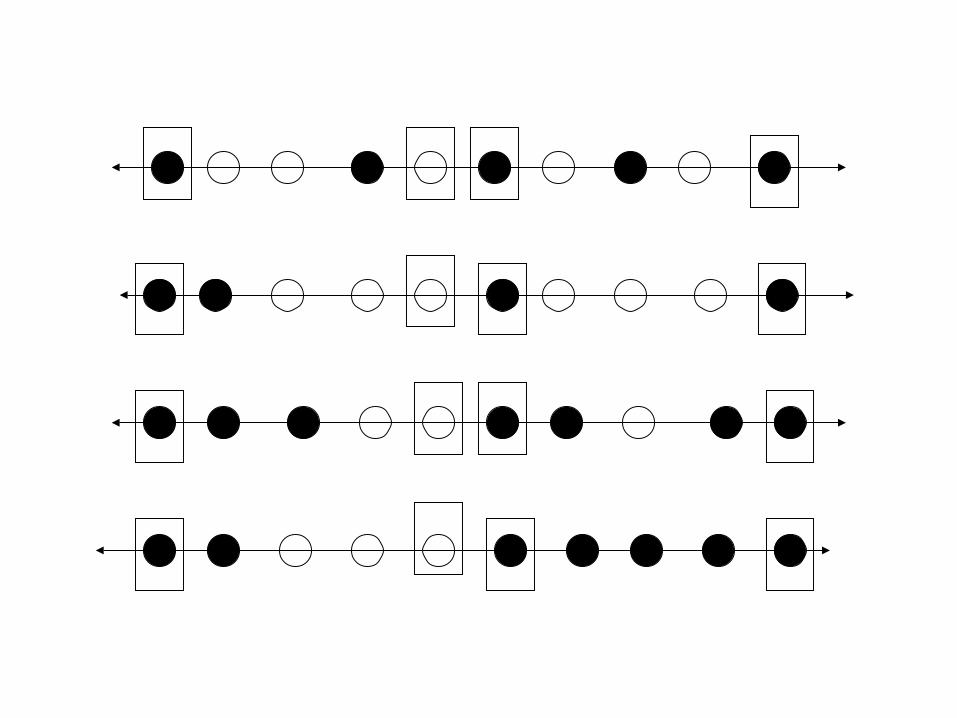
The Basic Model

• Individuals are either 0 or 1, either black or white

• They are on a lattice and occasionally imitate their neighors

• Some neighbors are fixed and never imitate (these are people with a high desire for crime or innocence)

• We look at long run behavior

v

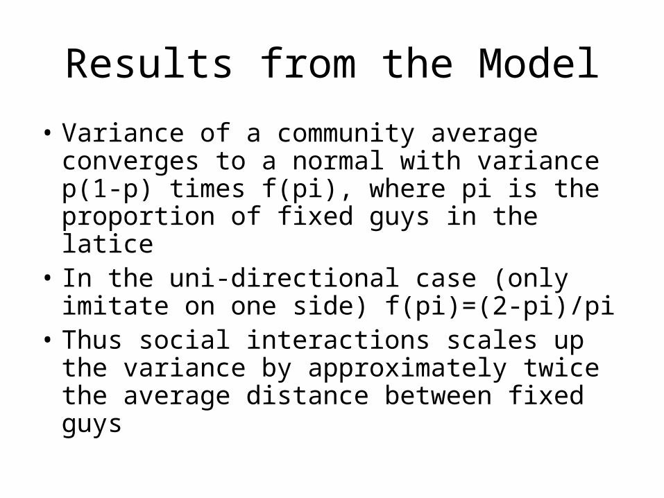
Results from the Model

• Variance of a community average converges to a normal with variance p(1-p) times f(pi), where pi is the proportion of fixed guys in the latice

• In the uni-directional case (only imitate on one side) f(pi)=(2-pi)/pi

• Thus social interactions scales up the variance by approximately twice the average distance between fixed guys

Excess Variance: Empirics

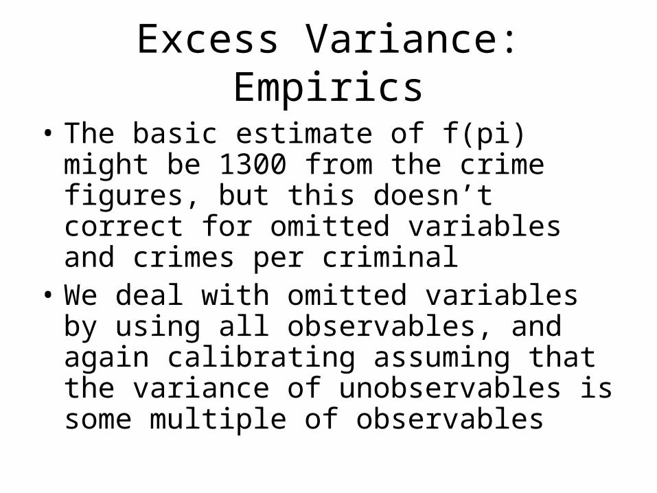
• The basic estimate of f(pi) might be 1300 from the crime figures, but this doesn’t correct for omitted variables and crimes per criminal

• We deal with omitted variables by using all observables, and again calibrating assuming that the variance of unobservables is some multiple of observables

Excess Variance Empirics

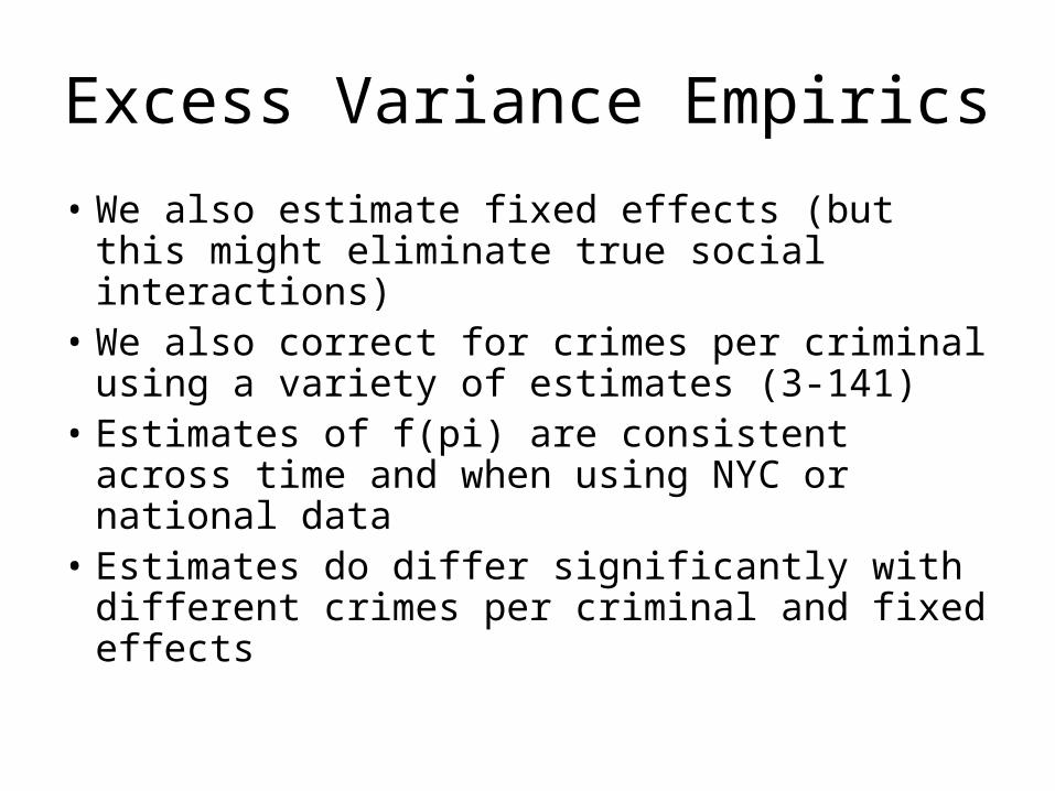
• We also estimate fixed effects (but this might eliminate true social interactions)

• We also correct for crimes per criminal using a variety of estimates (3-141)

• Estimates of f(pi) are consistent across time and when using NYC or national data

• Estimates do differ significantly with different crimes per criminal and fixed effects

Results

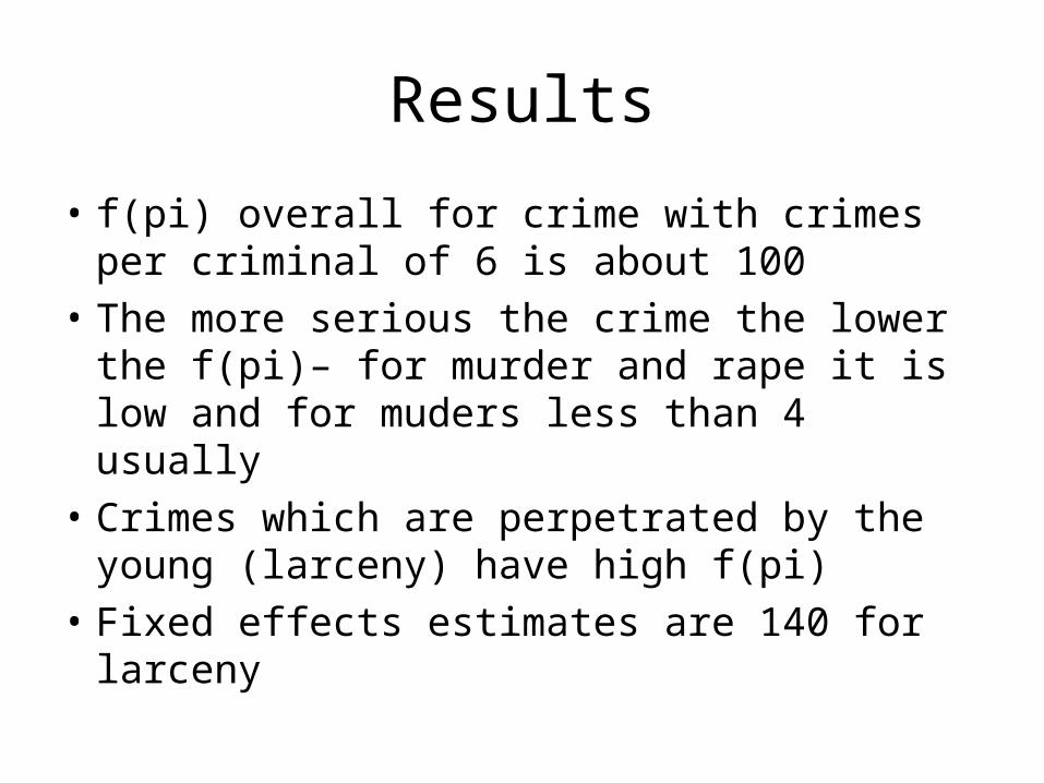
• f(pi) overall for crime with crimes per criminal of 6 is about 100

• The more serious the crime the lower the f(pi)– for murder and rape it is low and for muders less than 4 usually

• Crimes which are perpetrated by the young (larceny) have high f(pi)

• Fixed effects estimates are 140 for larceny

Issues with Excess Variance Empirics

• This approach does not avoid the problems with estimating social interactions (except # 1)

• Unobserved heterogeneity is a particular problem– we try to estimate this directly and then calibrate

• We also use functional form and the scaling property to test this

The Social Multiplier

• Basic Idea– The presence of social interactions means that macro-elasticities will be bigger than micro-elasticities because the macro estimates include spillovers

• Modest interpretation: macro-estimates, and all state-level regressions are biased and estimating a combination of micro-coefficient and social multiplier

• Aggressive interpretation: we can actually estimate spillovers

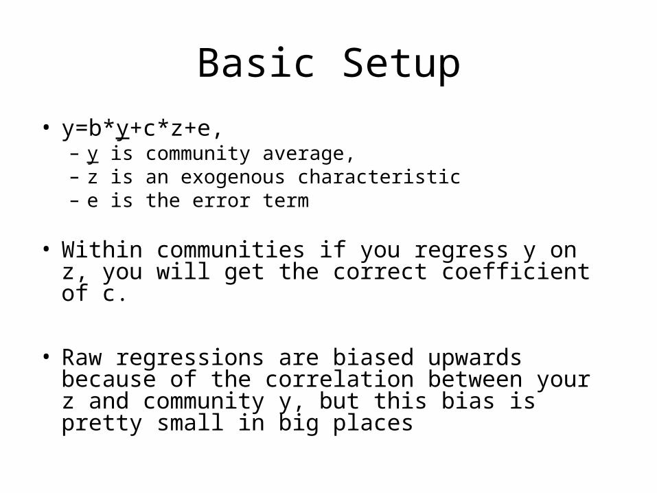
Basic Setup

• y=b*y+c*z+e,– y is community average, – z is an exogenous characteristic – e is the error term

• Within communities if you regress y on z, you will get the correct coefficient of c.

• Raw regressions are biased upwards because of the correlation between your z and community y, but this bias is pretty small in big places

Social Multiplier Theory

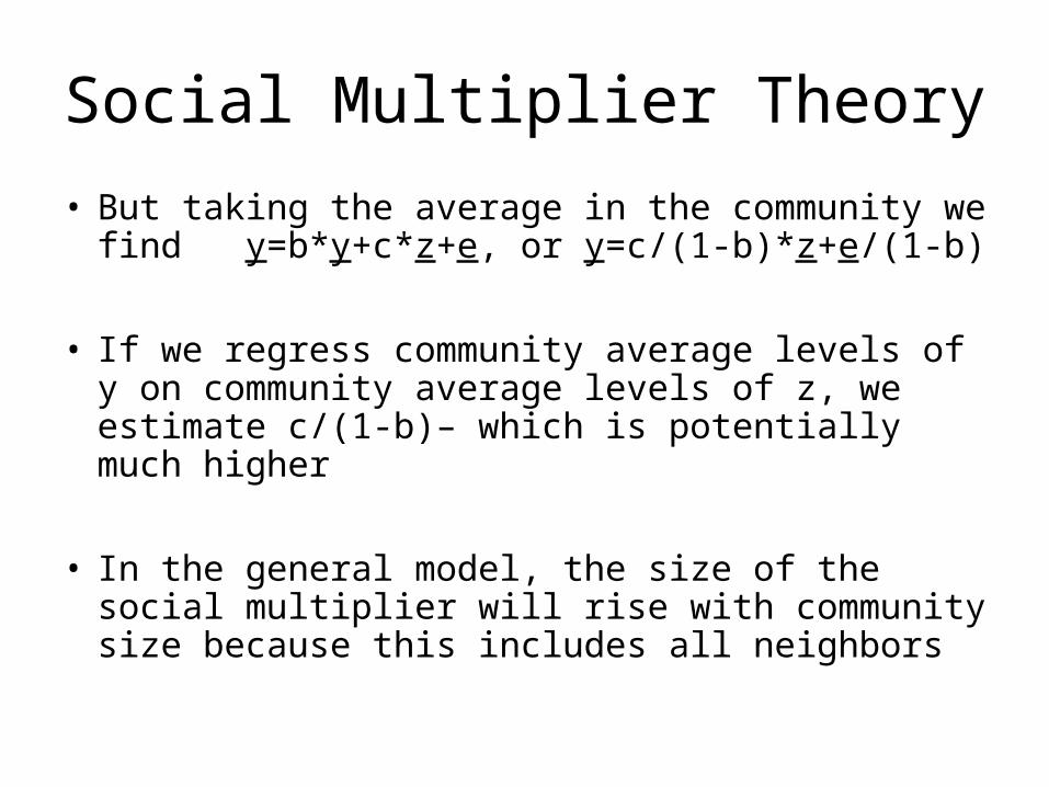
• But taking the average in the community we find y=b*y+c*z+e, or y=c/(1-b)*z+e/(1-b)

• If we regress community average levels of y on community average levels of z, we estimate c/(1-b)– which is potentially much higher

• In the general model, the size of the social multiplier will rise with community size because this includes all neighbors

Social Multiplier Empirics

• Dartmouth roommates estimates of joing a fraternity of drinking beer in high school– coefficient rises from .1 to .15 to .23 moving from individual to floor to dorm

• With multiple z’s it may make sense to first estimate “c” from micro-regressions and then regress y on cz the resulting coefficient is 1/(1-b)– the multiplier

More Social Multiplier Empirics

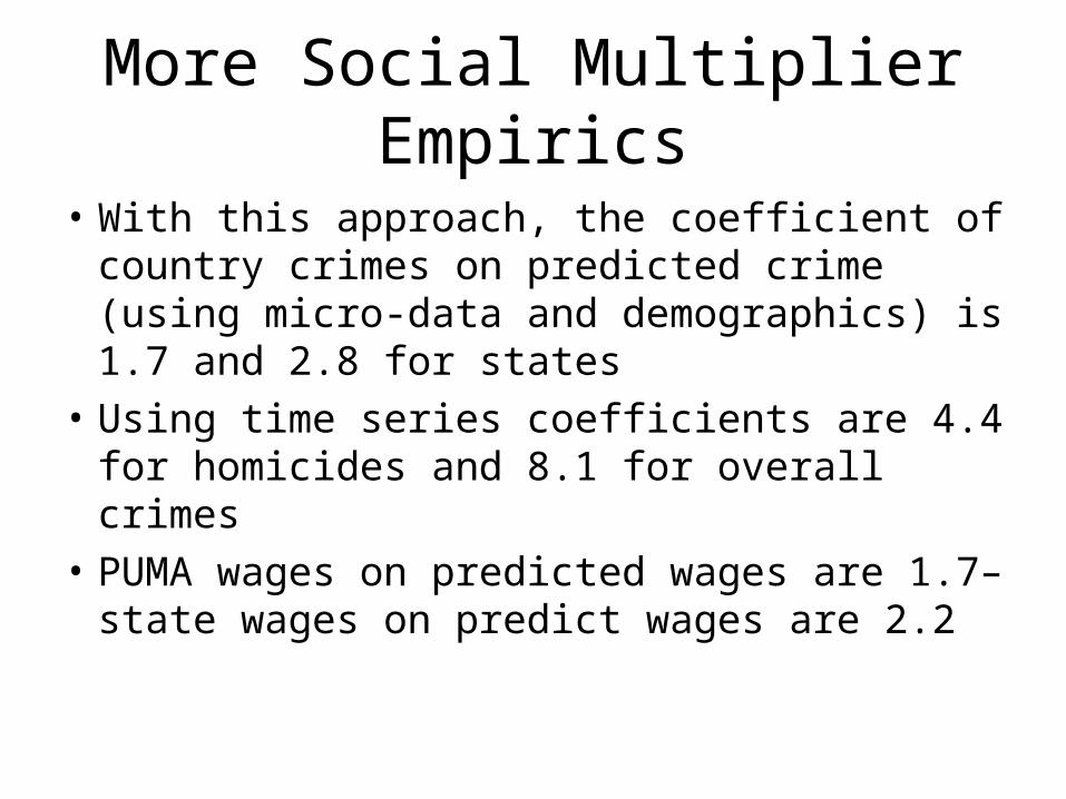
• With this approach, the coefficient of country crimes on predicted crime (using micro-data and demographics) is 1.7 and 2.8 for states

• Using time series coefficients are 4.4 for homicides and 8.1 for overall crimes

• PUMA wages on predicted wages are 1.7– state wages on predict wages are 2.2

Segregation in Cities

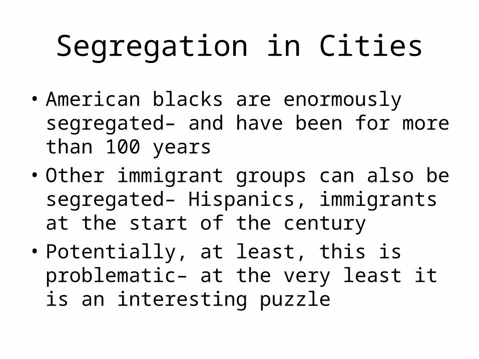
• American blacks are enormously segregated– and have been for more than 100 years

• Other immigrant groups can also be segregated– Hispanics, immigrants at the start of the century

• Potentially, at least, this is problematic– at the very least it is an interesting puzzle

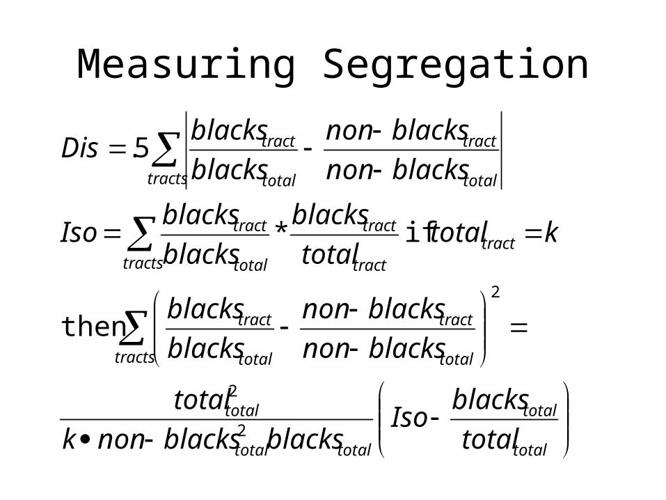
Measuring Segregation

total

total

totaltotal

total

tracts total

tract

total

tract

tracttracts tract

tract

total

tract

tracts total

tract

total

tract

total

blacksIso

blacksblacksnonk

total

blacksnon

blacksnon

blacks

blacks

ktotaltotal

blacks

blacks

blacksIso

blacksnon

blacksnon

blacks

blacksDis

2

2

2

then

if *

5.

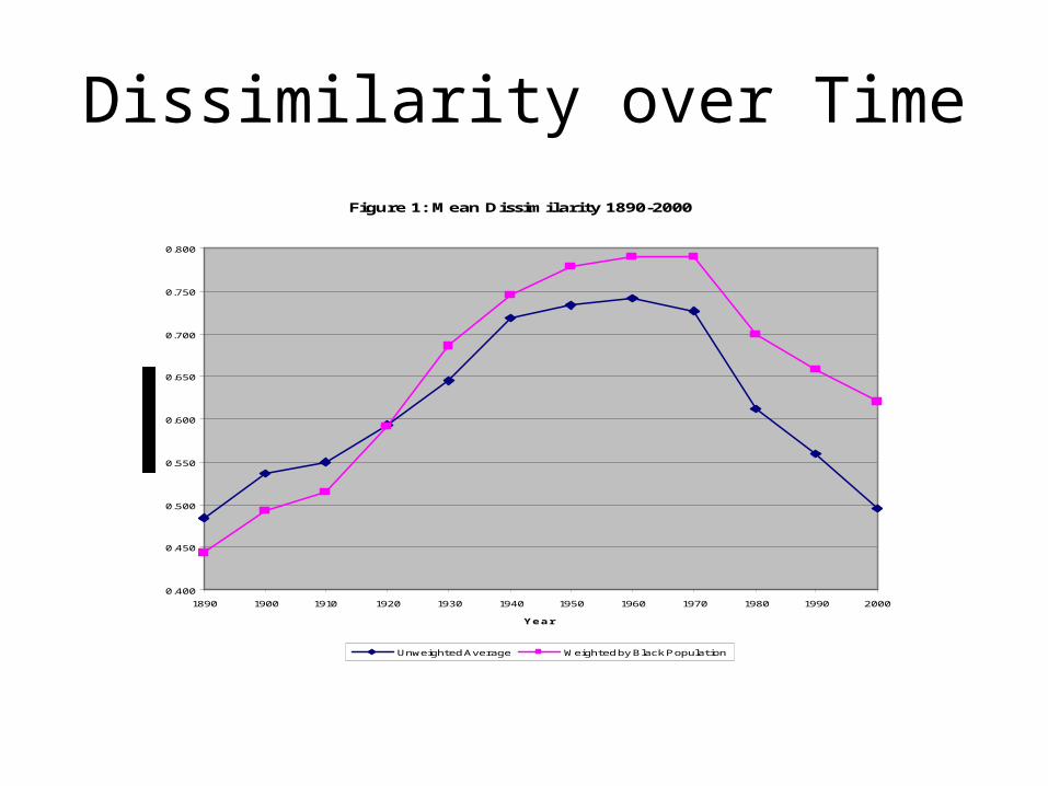
Dissimilarity over TimeFigure 1: Mean Dissimilarity 1890-2000

0.400

0.450

0.500

0.550

0.600

0.650

0.700

0.750

0.800

1890 1900 1910 1920 1930 1940 1950 1960 1970 1980 1990 2000

Year

Unweighted Average Weighted by Black Population

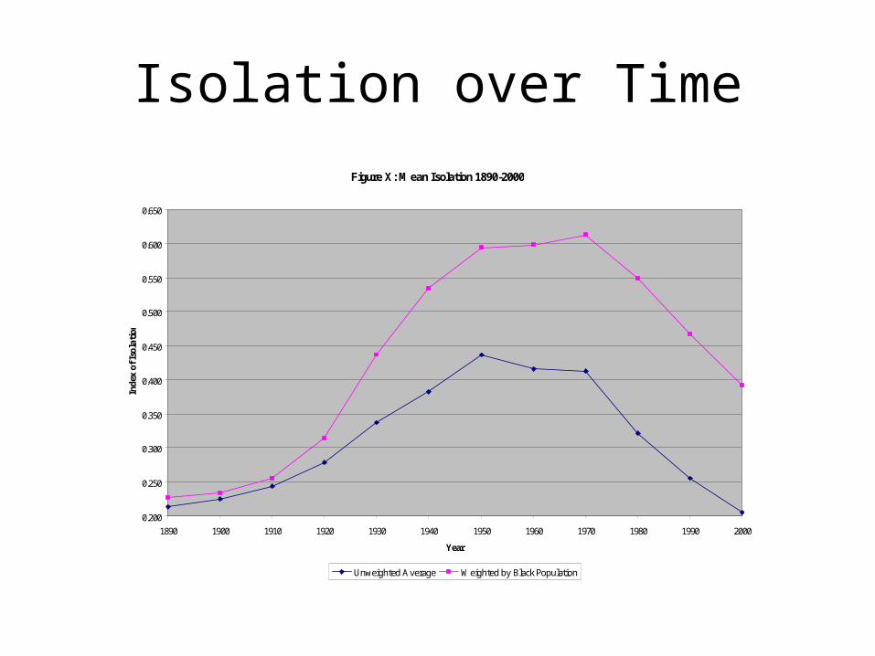
Isolation over Time

Figure X: Mean Isolation 1890-2000

0.200

0.250

0.300

0.350

0.400

0.450

0.500

0.550

0.600

0.650

1890 1900 1910 1920 1930 1940 1950 1960 1970 1980 1990 2000

Year

Inde

x of

Iso

lati

on

Unweighted Average Weighted by Black Population

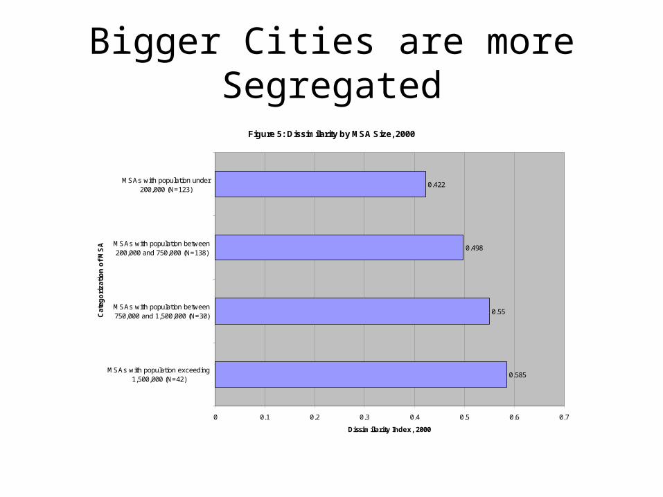
Bigger Cities are more Segregated

Figure 5: Dissimilarity by MSA Size, 2000

0.585

0.55

0.498

0.422

0 0.1 0.2 0.3 0.4 0.5 0.6 0.7

MSAs with population exceeding1,500,000 (N=42)

MSAs with population between750,000 and 1,500,000 (N=30)

MSAs with population between200,000 and 750,000 (N=138)

MSAs with population under200,000 (N=123)

Cat

ego

riza

tio

n o

f M

SA

Dissimilarity Index, 2000

Other Facts about Segregation

• The Midwest is the most segregated region, followed by the Northeast, the South and the West.

• Segregation is highly persistent, Cleveland and Chicago were among the 5 most segregated cities for 100 years.

• Education blacks are much less segregated than non-educated blacks today (.69 vs. 54 in 90), but not in 1970 (.76 vs .74)

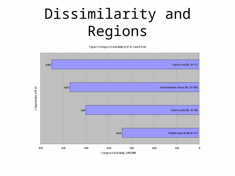
Dissimilarity and RegionsFigure 2: Changes in Dissimilarity by MSA Growth Rate

-0.034

-0.05

-0.057

-0.065

-0.07 -0.06 -0.05 -0.04 -0.03 -0.02 -0.01 0

Negative growth rate (N=21)

Growth under 10% (N=90)

Growth between 10 and 25% (N=109)

Growth over 25% (N=71)

Cat

egor

izat

ion

of M

SA

Change in Dissimilarity, 1990-2000

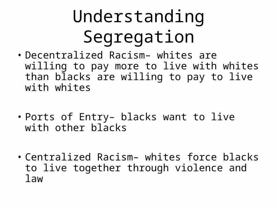
Understanding Segregation

• Decentralized Racism– whites are willing to pay more to live with whites than blacks are willing to pay to live with whites

• Ports of Entry– blacks want to live with other blacks

• Centralized Racism– whites force blacks to live together through violence and law

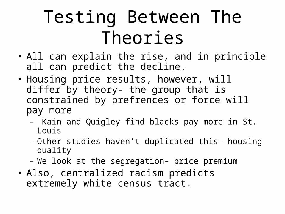
Testing Between The Theories

• All can explain the rise, and in principle all can predict the decline.

• Housing price results, however, will differ by theory– the group that is constrained by prefrences or force will pay more– Kain and Quigley find blacks pay more in St. Louis– Other studies haven’t duplicated this– housing quality– We look at the segregation– price premium

• Also, centralized racism predicts extremely white census tract.

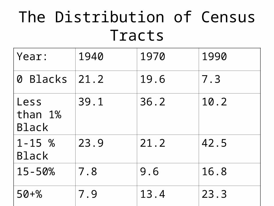
The Distribution of Census Tracts

Year: 1940 1970 1990

0 Blacks 21.2 19.6 7.3

Less than 1% Black

39.1 36.2 10.2

1-15 % Black

23.9 21.2 42.5

15-50% 7.8 9.6 16.8

50+% 7.9 13.4 23.3

Segregation and Housing Prices

• Ln(Rent)=a+b*Black+c*Black*Segregation+Other controls for city and unit

• In 1940, rental coefficient on black is -1.4(.36), interaction is 1.3(.5)

• In 1970, coefficient on black is -.42(.13) interaction is .38(.16)

• In 1990, coefficient on black is .15(.07) interaction is -.38(.1)

Segregation and Attitudes

• The General Social Survey collects information on opinions on race

• In more segregated cities, blacks are more likely to say that they prefer white neighborhoods (not significant)

• In more segregated cities, whites say that they believe in the right to segregation and support a ban on interracial marriage

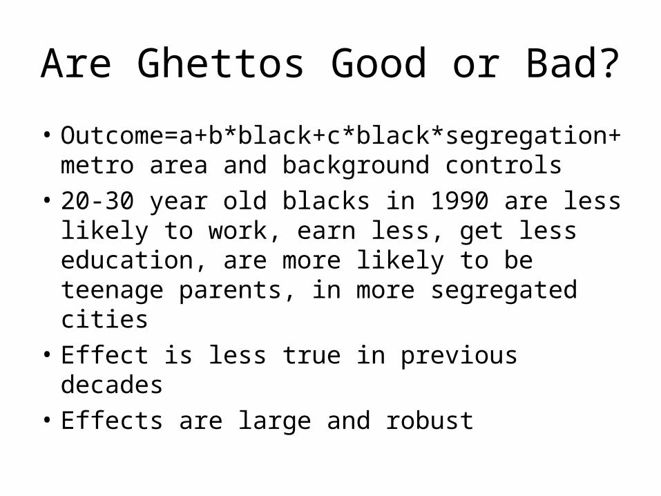
Are Ghettos Good or Bad?

• Outcome=a+b*black+c*black*segregation+metro area and background controls

• 20-30 year old blacks in 1990 are less likely to work, earn less, get less education, are more likely to be teenage parents, in more segregated cities

• Effect is less true in previous decades

• Effects are large and robust

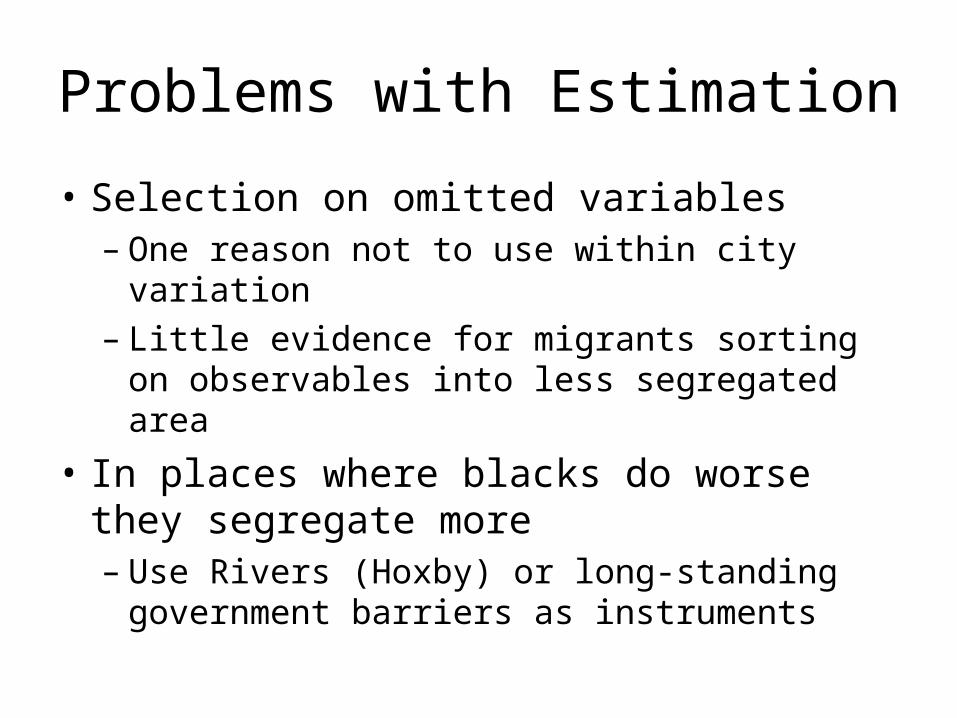
Problems with Estimation

• Selection on omitted variables– One reason not to use within city variation – Little evidence for migrants sorting on

observables into less segregated area

• In places where blacks do worse they segregate more– Use Rivers (Hoxby) or long-standing

government barriers as instruments

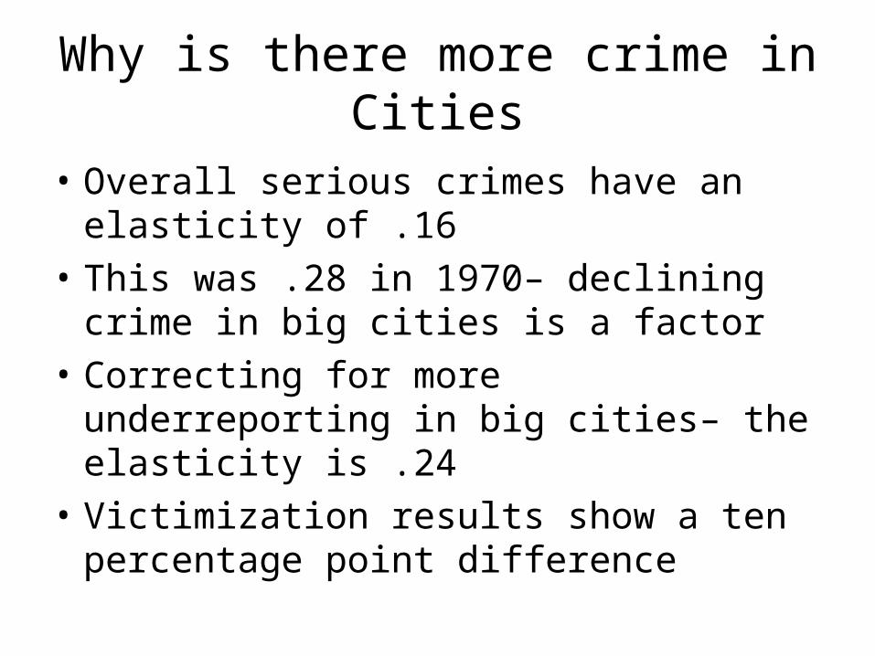
Why is there more crime in Cities

• Overall serious crimes have an elasticity of .16

• This was .28 in 1970– declining crime in big cities is a factor

• Correcting for more underreporting in big cities– the elasticity is .24

• Victimization results show a ten percentage point difference

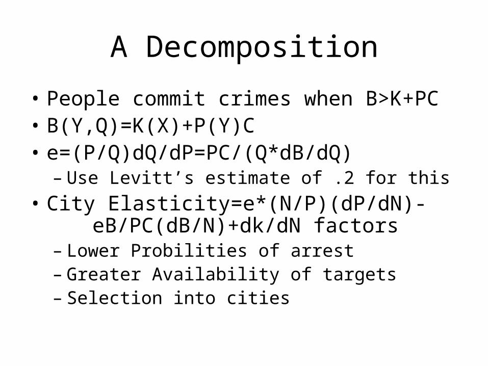
A Decomposition

• People commit crimes when B>K+PC• B(Y,Q)=K(X)+P(Y)C• e=(P/Q)dQ/dP=PC/(Q*dB/dQ)

– Use Levitt’s estimate of .2 for this

• City Elasticity=e*(N/P)(dP/dN)-eB/PC(dB/N)+dk/dN factors– Lower Probilities of arrest– Greater Availability of targets– Selection into cities

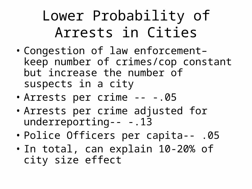
Lower Probability of Arrests in Cities

• Congestion of law enforcement– keep number of crimes/cop constant but increase the number of suspects in a city

• Arrests per crime -- -.05• Arrests per crime adjusted for

underreporting-- -.13• Police Officers per capita-- .05• In total, can explain 10-20% of city size

effect

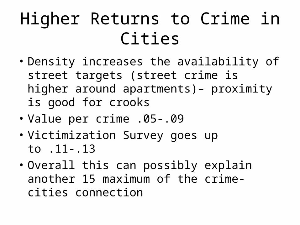
Higher Returns to Crime in Cities

• Density increases the availability of street targets (street crime is higher around apartments)– proximity is good for crooks

• Value per crime .05-.09

• Victimization Survey goes up to .11-.13

• Overall this can possibly explain another 15 maximum of the crime-cities connection

Social Heterogeneity in Cities

• The city size effect disappears when we control for percent single parent family

• What does this mean– maybe this is itself a result of social disfunction

• Instrument using AFDC laws interacted with poverty rate in 1970

• This can explain the remaining ½ of the city size effect

• This also reflects the social multiplier

The Economics of Punishment

• The basic model is a positive theory of crime, a normative theory of punishment

• But punishment itself is less than optimal and worth trying to understand

• There are several different levels of choice involved– Choice of laws and rules– Choices by judges and prosecutors

What do Prosecutors Maximize (ALER with Kessler and Piehl)

• In the U.S., in crimes which are both federal and state, federal attorneys essentially get to choose who to go after

• They chose to go after people without records, who are rich, white, likely to have private attorneys, nonviolent– Career concerns, i.e. skills, connections– Even true among possession cases

• This may be socially beneficial if you need good federal attorneys to beat good private attorneys, but may also be bad

Sentencing for Homicides

Optimal Sentencing might minimizeN(PL)*(PCL+V)

N is number of crimesP is probability of being caughtC is social cost of sentenceL is sentence lengthV is cost of crime occuringN’(PL)<0

Optimal Sentencing

-N’(PL)*P(PCL+V)=N(PL)*PC or eV=(1-e)PCL where e is supply elasticity or Log(L)=Log(V)+Log(e/(1-e))+Log(P)+Log(C) • Facts about sentencing across murders

– The probability of being caught fact is about right

– The supply elasticities are hard to measure, but seem close to right

– Little victim effects

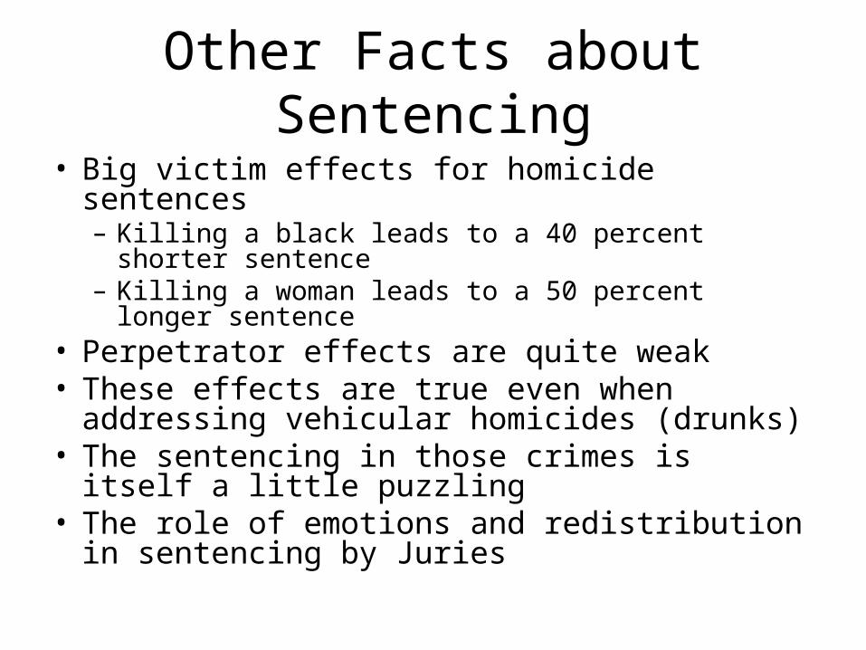
Other Facts about Sentencing

• Big victim effects for homicide sentences– Killing a black leads to a 40 percent shorter sentence– Killing a woman leads to a 50 percent longer

sentence• Perpetrator effects are quite weak• These effects are true even when addressing

vehicular homicides (drunks)• The sentencing in those crimes is itself a little

puzzling• The role of emotions and redistribution in

sentencing by Juries

The Theory of Punishment

• Key Insight of Public Choice – design rules to deal with incentives by implementers

• Bureaucrats vs. Independents (English vs. French)– check against gov’t vs. laziness

• Judicial Codes– good for controlling independent judges

• Quantity controls make things easier to monitor

Riots (JUE, 1998)

• Generally an urban phenomenon– rural uprisings were easier to suppress

• Important both because of the raw damage and because of regime change

• Basic model is getting enough people to overwhelm the police

• Initial crowds• Emotional Minority• Organization

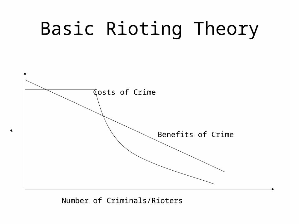
Basic Rioting Theory

Benefits of Crime

Costs of Crime

Number of Criminals/Rioters

Facts about Riots

• Across countries US + India have the most riots

• Increases with ethnic heterogeneity, urbanization and the interactions

• Decreases in Dictatorships

• Decreases with GDP

In the U.S.

• In the 60s and today, little correlation with poverty

• Homeownership decreases riot occurrence rates in the 60s

• South had fewer riots• In places with more cops, riots were less

severe• Big variable is size of the non-white

communit

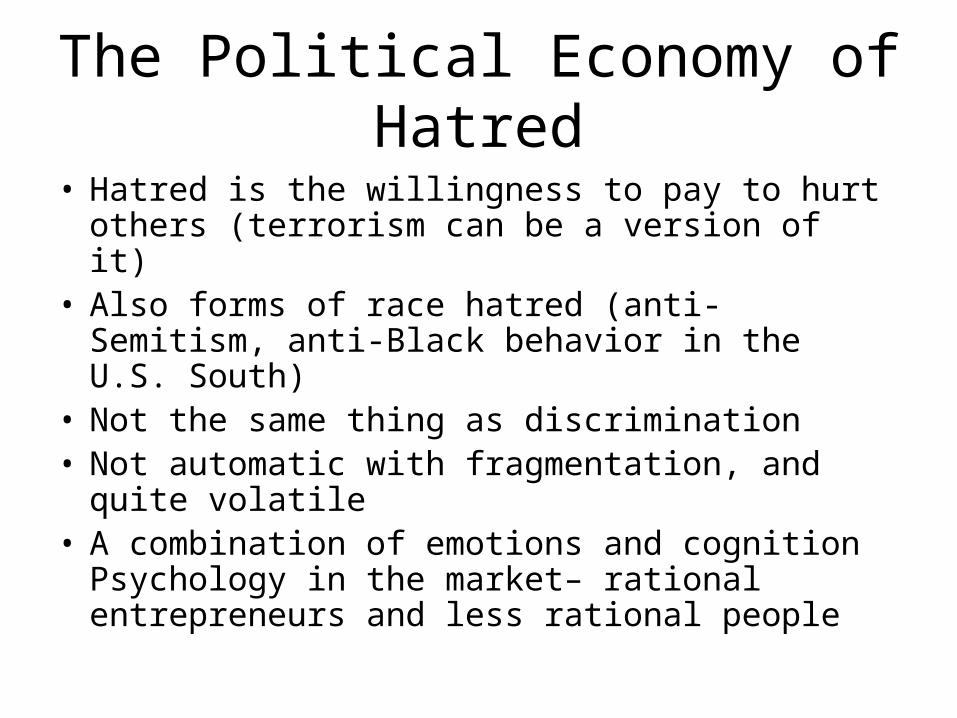
The Political Economy of Hatred

• Hatred is the willingness to pay to hurt others (terrorism can be a version of it)

• Also forms of race hatred (anti-Semitism, anti-Black behavior in the U.S. South)

• Not the same thing as discrimination• Not automatic with fragmentation, and quite

volatile• A combination of emotions and cognition

Psychology in the market– rational entrepreneurs and less rational people

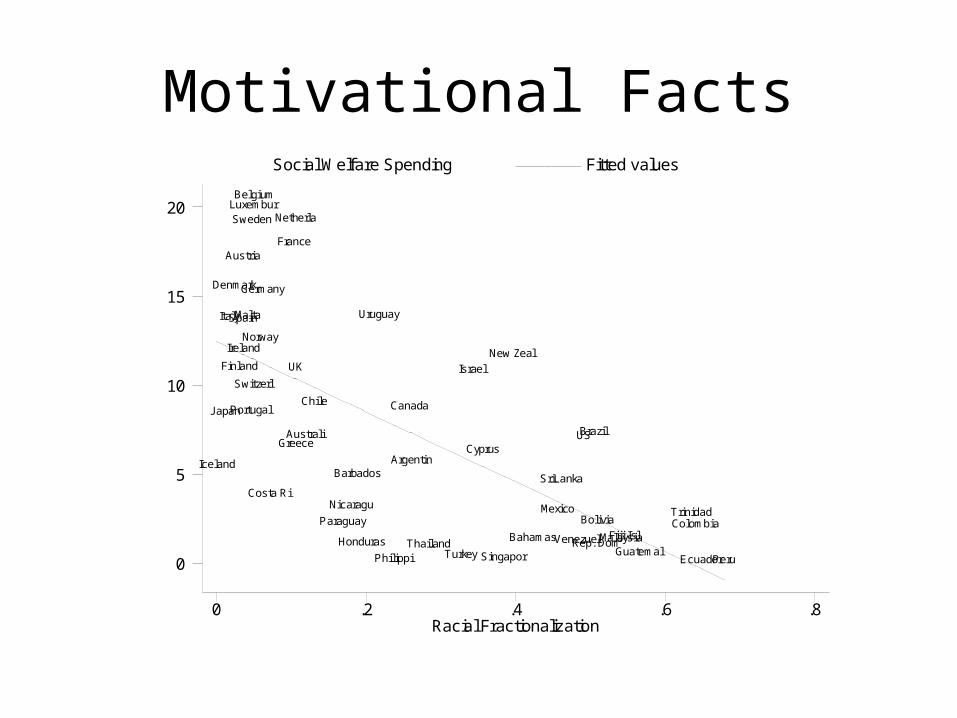
Motivational Facts

Racial Fractionalization

Social Welfare Spending Fitted values

0 .2 .4 .6 .8

0

5

10

15

20

Iceland

Japan

Italy

Denmark

Finland

Austria

Spain

Ireland

Malta

Portugal

Sweden

BelgiumLuxembur

Switzerl

Norway

Germany

Costa Ri

France

UK

Netherla

GreeceAustrali

Chile

Paraguay

Nicaragu

Barbados

Honduras

Uruguay

Philippi

Canada

Argentin

ThailandTurkey

Israel

Cyprus

Singapor

New Zeal

Bahamas

Mexico

SriLanka

Venezuel

US

Rep. Dom

Brazil

Bolivia

MalaysiaFiji Isl

Guatemal

TrinidadColombia

EcuadorPeru

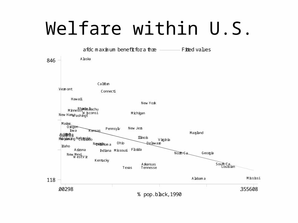
Welfare within U.S.

% pop. black, 1990

afdc maximum benef it for a thre Fitted values

.00298 .355608

118

846

Alabama

Alaska

Arizona

Arkansas

Californ

Colorado

Connecti

Delaware

FloridaGeorgia

Hawaii

Idaho

Illinois

Indiana

Iowa Kansas

Kentucky

Louisian

Maine

Maryland

MassachuMichigan

Minnesot

Mississi

Missouri

Montana Nebraska

Nevada

New Hamp

New Jers

New Mexi

New York

North Ca

North Da

OhioOklahoma

Oregon Pennsylv

Rhode Is

South Ca

South Da

TennesseTexas

Utah

Vermont

Virginia

Washingt

West Vir

Wisconsi

Wyoming

Anti Americanism around the World

• Please tell me if you have a very favorable, somewhat favorable, somewhat unfavorable or very unfavorable opinion of the United States

• Vietnam 4% very vs. 8% for France and Canada (27 vs. 34 and 27 including somewhat

• Argentina 23 % very vs. 3% Guatemala and 2% Honduras (49 vs. 13 and 5)

Anti Americanism and Islam

muslims as % pop 1980 w ce95

Highly Unfavorable to U.S. Fitted values

0 99.8

1

59

ItalyGermany

France

UKHonduras

Philippi

Canada

Argentin

Turkey

Mexico

Venezuel

Brazil

Bolivia

Guatemal

India

Peru

South Af

RussiaVietnam

SlovakiaCote d'I

Banglade

Egypt

AngolaUganda

Nigeria

Jordan

Tanzania

KenyaGhana

Pakistan

Uzbejist

BulgariaSouth Ko

Mali

Lebanon

Ukrania

Indonesi

Poland

Emotional Roots of Hatred

• Asdasd

• Chemicals

• Ultimatum Games

• Murders, Riots, Gangs and Vengeance

The Formation of Hatred

• Hatred is always and everywhere formed by stories of past and future atrocities– Tales of Blacks raping white girls in the South– Tales of Jews killing Jesus, drinking children’s blood,

and the Protocols of the Elders of Zion– America and the Child in Barcelona

• Often these stories need repetition more than truth– Or sometimes they are true, but that group isn’t

particularly guilty

The Role of Political Entrepreneurs

• White conservatives in the south pushed race hatred in the 1880s and 1890s

• Right wing politicians in Europe (Lueger, Schonerer, Hitler) pushed anti-Semitism

• So did the Czar (Ochrana gave us the Protocols)

• Today, anti-Americanism is also used by different political groups

The Model

• The setting two parties competing for votes and sending out messages of hate

• Voters may investigate, form opinions about the dangers of an out-group

• Voters choose between the candidate

• In-group voters choose whether or not to isolate themselves from the out-group

• Contact with out-group might occur

Key decisions recursively

• Will in-group members isolate themselves– Only when they have heard a hate creating message

and not investigated• Which candidate will voters support

– They vote their pocketbook except – When they have heard a hate creating message and

not investigated and then they are more likely to favor policies that hurt the minority

• Will voters investigate the message– If it will change their isolation behavior

• Will politicians send hate creating messages– If it will increase votes

Key Comparative Statics

• Private individuals are more likely to investigate hate-creating messages when– The minority group is large– The minority group isn’t segregated– The potential harm is large and the gains from

self-protection are high

• Politicians are more likely to send a hate creating message when – This message is unlikely to be investigated

Comparative Statics on Supplying Hatred

• Hatred will be more likely to be supplied when the group is potentially more of a threat (holding search constant)

• Hatred is more likely when the group is different along the policy-relevant dimension

• The right pushes hate against poor minorities the left against rich minorities

Other Results

• With two issues the key is whether the group is policy relevant

• More extremism on the issue that the out-group is different on leads to more hatred

• Hating the haters can be an effective strategy

• Policies related to migration or segregation are natural complements to hatred

Understanding why race hatred rises between 1870 and 1910

• In the 1880s, depression created fertile ground for the first American party, the Populists, committed to redistribution from rich to poor.

• “More important to the success of Southern Populism than the combination with the West or with labor was the alliance with the Negro… Populists of other Southern states followed the example of Texas, electing Negroes to their councils and giving them a voice in the party organization.” (Woodward)

• “I have no words which can portray my contempt for the white men, Anglo-Saxons, who can knock their knees together, and through their chattering teeth and pale lips admit that they are afraid the Negroes will ‘dominate us.’” (Watson)

But the response was

• “Alarmed by the success that the Populists were enjoying with their appeal to the Negro voter, the conservatives themselves raised the cry of ‘Negro domination,’ and white supremacy, and enlisted the Negrophobe elements”

• “In Georgia and elsewhere the propaganda was furthered by a sensational press that played up and headlined current stories of Negro crime, charges of rape and attempted rape, and alleged instances of arrogance … already cowed and intimidated, the race was falsely pictured as stirred up to a mutinous and insurrectionary pitch” (both from Woodward)

Decline of Race Hatred

• Tom Watson by 1906 said the black man “grows more bumptious on the street, more impudent in his dealings with white men, and then, when he cannot achieve social equality as he wishes, with the instinct of the barbarian to destroy what he cannot attain to, he lies in wait, as that dastardly brute did yesterday near this city, and assaults the fair young girlhood of the south...”

• Key lessons– strategic, related to policy relevance, not related to truth

Anti-Semitism in 19th Century Europe

• Political, not religious, and big in Russia, Germany, Austria, mixed in France

• Not in U.S., U.K., Italy or Spain• Key ideological divide in the first country is king

vs. constitutionalism (Kaiser in 1871)• The Austrian empire “a political system so

flagrantly out of step with the spirit of the times needed at least one strong ideological ally; this ally by a process of elimination could only be the Church.” (Kann)

19th Century Anti-Semitism

• Cohn (1956) wrote “the Right (conservative, monarchical, ‘clerical’) maintained that there must be a place for the Church in the public order; the Left (democratic, liberal, radical) held that there can be no (public) Church at all.”

• And “Jews supported the Left, then, not only because they had become unshakeable partisans of the Emancipation, but also because they had no choice; as far as the internal life of the Right was concerned, the Emancipation had never taken place, and the Christian religion remained a prerequisite for political participation.”

If Jews are on the left, then right wing anti-Semitism follows

• “from Stoecker to Hitler, rightists rarely attempted to refute socialism, preferring to cite the high percentage of intellectuals of Jewish origin among socialist publicists as proof of its subversion” (Weiss, 1996).

• In 1892, the conservative party platform embraced anti-Semitism and pledged to “do battle against the many-sided aggressive, decomposing, and arrogant Jewish influence on the life of our people” (Weiss, 1996, p. 116).

Russia, Austria and France

• In Russia, the Czar used anti-Semitism to build up support for his pro-Church regime

• In Austria, anti-Semitism was actually used against the Emperor by Lueger

• In France, the right wing tried (Dreyfus) but were defeated by left wing strength– Zola describes the War Office that convicted

Dreyfus as a “nest of Jesuits” prone to “inquisitorial and tyrannical methods.”

Italy and Spain

• Spain’s easy– no Jews post 1492 (or at least 1600)– There was some anti-Masonic hatred that

played a similar role (also in U.S.)

• Italy is more interesting– the modern state was founded on expropriation of the Pope– As such, the king and everyone in politics was

excommunicated– As such, there was no church in politics, and

Jews weren’t policy relevant

U.S. and U.K.

• Divine right monarchies and church and state issues were settled long before the 19th century

• As a result, Jews weren’t particularly policy relevant and occupied both sides of the political aisle

• Disraeli and Judah Benjamin