Embed Size (px)
Citation preview
Numerical Differentiation & Integration
Gaussian Quadrature
Numerical Analysis (9th Edition)
R L Burden & J D Faires
Beamer Presentation Slidesprepared byJohn Carroll
Dublin City University
c© 2011 Brooks/Cole, Cengage Learning

Introduction Legendre Polynomials Arbitrary Intervals
Outline
1 Gaussian Quadrature & Optimal Nodes
Numerical Analysis (Chapter 4) Gaussian Quadrature R L Burden & J D Faires 2 / 40
Introduction Legendre Polynomials Arbitrary Intervals
Outline
1 Gaussian Quadrature & Optimal Nodes
2 Using Legendre Polynomials to Derive Gaussian Quadrature Formulae
Numerical Analysis (Chapter 4) Gaussian Quadrature R L Burden & J D Faires 2 / 40
Introduction Legendre Polynomials Arbitrary Intervals
Outline
1 Gaussian Quadrature & Optimal Nodes
2 Using Legendre Polynomials to Derive Gaussian Quadrature Formulae
3 Gaussian Quadrature on Arbitrary Intervals
Numerical Analysis (Chapter 4) Gaussian Quadrature R L Burden & J D Faires 2 / 40
Introduction Legendre Polynomials Arbitrary Intervals
Outline
1 Gaussian Quadrature & Optimal Nodes
2 Using Legendre Polynomials to Derive Gaussian Quadrature Formulae
3 Gaussian Quadrature on Arbitrary Intervals
Numerical Analysis (Chapter 4) Gaussian Quadrature R L Burden & J D Faires 3 / 40
Introduction Legendre Polynomials Arbitrary Intervals
Gaussian Quadrature: Contrast with Newton-Cotes
Features of a Newton-Cotes Formula
Numerical Analysis (Chapter 4) Gaussian Quadrature R L Burden & J D Faires 4 / 40
Introduction Legendre Polynomials Arbitrary Intervals
Gaussian Quadrature: Contrast with Newton-Cotes
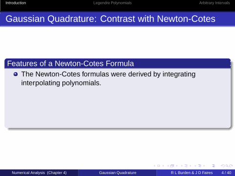
Features of a Newton-Cotes FormulaThe Newton-Cotes formulas were derived by integratinginterpolating polynomials.
Numerical Analysis (Chapter 4) Gaussian Quadrature R L Burden & J D Faires 4 / 40
Introduction Legendre Polynomials Arbitrary Intervals
Gaussian Quadrature: Contrast with Newton-Cotes
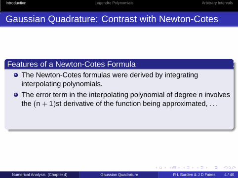
Features of a Newton-Cotes FormulaThe Newton-Cotes formulas were derived by integratinginterpolating polynomials.
The error term in the interpolating polynomial of degree n involvesthe (n + 1)st derivative of the function being approximated, . . .
Numerical Analysis (Chapter 4) Gaussian Quadrature R L Burden & J D Faires 4 / 40
Introduction Legendre Polynomials Arbitrary Intervals
Gaussian Quadrature: Contrast with Newton-Cotes
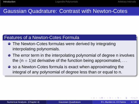
Features of a Newton-Cotes FormulaThe Newton-Cotes formulas were derived by integratinginterpolating polynomials.
The error term in the interpolating polynomial of degree n involvesthe (n + 1)st derivative of the function being approximated, . . .
so a Newton-Cotes formula is exact when approximating theintegral of any polynomial of degree less than or equal to n.
Numerical Analysis (Chapter 4) Gaussian Quadrature R L Burden & J D Faires 4 / 40
Introduction Legendre Polynomials Arbitrary Intervals
Gaussian Quadrature: Contrast with Newton-Cotes
Features of a Newton-Cotes Formula (Cont’d)
Numerical Analysis (Chapter 4) Gaussian Quadrature R L Burden & J D Faires 5 / 40
Introduction Legendre Polynomials Arbitrary Intervals
Gaussian Quadrature: Contrast with Newton-Cotes
Features of a Newton-Cotes Formula (Cont’d)All the Newton-Cotes formulas use values of the function atequally-spaced points.
This restriction is convenient when the formulas are combined toform the composite rules which we considered earlier, . . .
but it can significantly decrease the accuracy of the approximation.
Numerical Analysis (Chapter 4) Gaussian Quadrature R L Burden & J D Faires 5 / 40
Introduction Legendre Polynomials Arbitrary Intervals
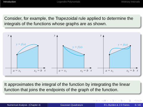
Consider, for example, the Trapezoidal rule applied to determine theintegrals of the functions whose graphs are as shown.
y
x
yy
xa 5 x1 a 5 x1 a 5 x1x2 5 b x2 5 b x2 5 bx
y 5 f (x)y 5 f (x)
y 5 f (x)
It approximates the integral of the function by integrating the linearfunction that joins the endpoints of the graph of the function.
Numerical Analysis (Chapter 4) Gaussian Quadrature R L Burden & J D Faires 6 / 40
Introduction Legendre Polynomials Arbitrary Intervals
Gaussian Integration: Optimal integration points
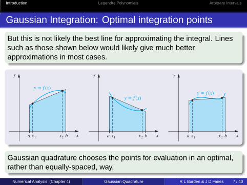
But this is not likely the best line for approximating the integral. Linessuch as those shown below would likely give much betterapproximations in most cases.
yyy
x x xa x1 bx2 a x1 bx2 a x1 bx2
y 5 f (x)
y 5 f (x)y 5 f (x)
Gaussian quadrature chooses the points for evaluation in an optimal,rather than equally-spaced, way.
Numerical Analysis (Chapter 4) Gaussian Quadrature R L Burden & J D Faires 7 / 40
Introduction Legendre Polynomials Arbitrary Intervals
Gaussian Quadrature: Introduction
Choice of Integration Nodes
Numerical Analysis (Chapter 4) Gaussian Quadrature R L Burden & J D Faires 8 / 40
Introduction Legendre Polynomials Arbitrary Intervals
Gaussian Quadrature: Introduction
Choice of Integration Nodes
The nodes x1, x2, . . . , xn in the interval [a, b] and coefficientsc1, c2, . . . , cn, are chosen to minimize the expected error obtainedin the approximation
∫ b
af (x) dx ≈
n∑
i=1
ci f (xi ).
To measure this accuracy, we assume that the best choice ofthese values produces the exact result for the largest class ofpolynomials, . . .
Numerical Analysis (Chapter 4) Gaussian Quadrature R L Burden & J D Faires 8 / 40

Introduction Legendre Polynomials Arbitrary Intervals
Gaussian Quadrature: Introduction
Choice of Integration Nodes
The nodes x1, x2, . . . , xn in the interval [a, b] and coefficientsc1, c2, . . . , cn, are chosen to minimize the expected error obtainedin the approximation
∫ b
af (x) dx ≈
n∑
i=1
ci f (xi ).
To measure this accuracy, we assume that the best choice ofthese values produces the exact result for the largest class ofpolynomials, . . .
that is, the choice that gives the greatest degree of precision.
Numerical Analysis (Chapter 4) Gaussian Quadrature R L Burden & J D Faires 8 / 40
Introduction Legendre Polynomials Arbitrary Intervals
Gaussian Quadrature: Introduction
∫ b
af (x) dx ≈
n∑
i=1
ci f (xi ).
Choice of Integration Nodes (Cont’d)
Numerical Analysis (Chapter 4) Gaussian Quadrature R L Burden & J D Faires 9 / 40

Introduction Legendre Polynomials Arbitrary Intervals
Gaussian Quadrature: Introduction
∫ b
af (x) dx ≈
n∑
i=1
ci f (xi ).
Choice of Integration Nodes (Cont’d)The coefficients c1, c2, . . . , cn in the approximation formula arearbitrary, and the nodes x1, x2, . . . , xn are restricted only by thefact that they must lie in [a, b], the interval of integration.
Numerical Analysis (Chapter 4) Gaussian Quadrature R L Burden & J D Faires 9 / 40
Introduction Legendre Polynomials Arbitrary Intervals
Gaussian Quadrature: Introduction
∫ b
af (x) dx ≈
n∑
i=1
ci f (xi ).
Choice of Integration Nodes (Cont’d)The coefficients c1, c2, . . . , cn in the approximation formula arearbitrary, and the nodes x1, x2, . . . , xn are restricted only by thefact that they must lie in [a, b], the interval of integration.
This gives us 2n parameters to choose.
Numerical Analysis (Chapter 4) Gaussian Quadrature R L Burden & J D Faires 9 / 40
Introduction Legendre Polynomials Arbitrary Intervals
Gaussian Quadrature: Introduction
∫ b
af (x) dx ≈
n∑
i=1
ci f (xi ).
Choice of Integration Nodes (Cont’d)
Numerical Analysis (Chapter 4) Gaussian Quadrature R L Burden & J D Faires 10 / 40
Introduction Legendre Polynomials Arbitrary Intervals
Gaussian Quadrature: Introduction
∫ b
af (x) dx ≈
n∑
i=1
ci f (xi ).
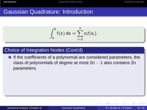
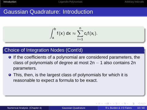
Choice of Integration Nodes (Cont’d)If the coefficients of a polynomial are considered parameters, theclass of polynomials of degree at most 2n − 1 also contains 2nparameters.
Numerical Analysis (Chapter 4) Gaussian Quadrature R L Burden & J D Faires 10 / 40
Introduction Legendre Polynomials Arbitrary Intervals
Gaussian Quadrature: Introduction
∫ b
af (x) dx ≈
n∑
i=1
ci f (xi ).
Choice of Integration Nodes (Cont’d)If the coefficients of a polynomial are considered parameters, theclass of polynomials of degree at most 2n − 1 also contains 2nparameters.
This, then, is the largest class of polynomials for which it isreasonable to expect a formula to be exact.
With the proper choice of the values and constants, exactness onthis set can be obtained.
Numerical Analysis (Chapter 4) Gaussian Quadrature R L Burden & J D Faires 10 / 40
Introduction Legendre Polynomials Arbitrary Intervals
Gaussian Quadrature: Illustration (n = 2)
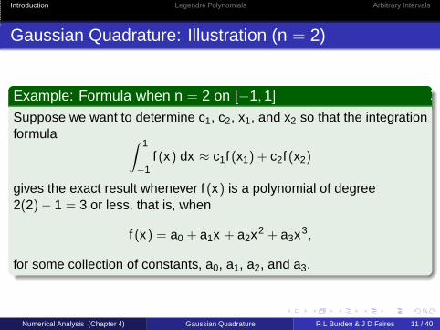
Example: Formula when n = 2 on [−1, 1]
Suppose we want to determine c1, c2, x1, and x2 so that the integrationformula
∫ 1
−1f (x) dx ≈ c1f (x1) + c2f (x2)
gives the exact result whenever f (x) is a polynomial of degree2(2) − 1 = 3 or less, that is, when
f (x) = a0 + a1x + a2x2 + a3x3,
for some collection of constants, a0, a1, a2, and a3.
Numerical Analysis (Chapter 4) Gaussian Quadrature R L Burden & J D Faires 11 / 40
Introduction Legendre Polynomials Arbitrary Intervals
Gaussian Quadrature: Illustration (n = 2)
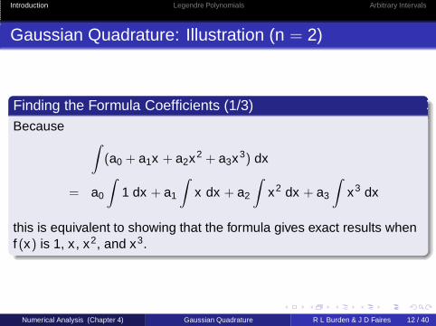
Finding the Formula Coefficients (1/3)Because
∫
(a0 + a1x + a2x2 + a3x3) dx
= a0
∫
1 dx + a1
∫
x dx + a2
∫
x2 dx + a3
∫
x3 dx
this is equivalent to showing that the formula gives exact results whenf (x) is 1, x , x2, and x3.
Numerical Analysis (Chapter 4) Gaussian Quadrature R L Burden & J D Faires 12 / 40
Introduction Legendre Polynomials Arbitrary Intervals
Gaussian Quadrature: Illustration (n = 2)
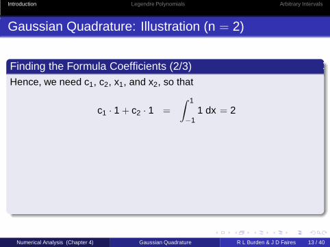
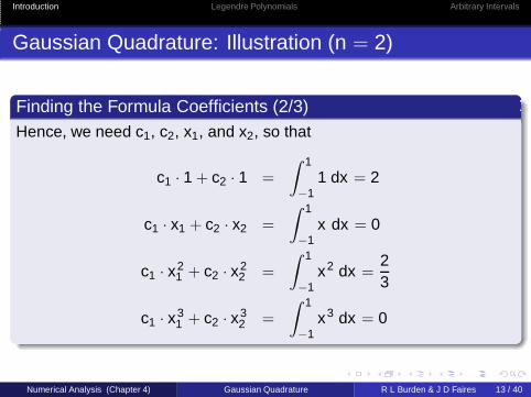
Finding the Formula Coefficients (2/3)Hence, we need c1, c2, x1, and x2, so that
c1 · 1 + c2 · 1 =
∫ 1
−11 dx = 2
Numerical Analysis (Chapter 4) Gaussian Quadrature R L Burden & J D Faires 13 / 40
Introduction Legendre Polynomials Arbitrary Intervals
Gaussian Quadrature: Illustration (n = 2)
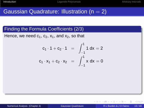
Finding the Formula Coefficients (2/3)Hence, we need c1, c2, x1, and x2, so that
c1 · 1 + c2 · 1 =
∫ 1
−11 dx = 2
c1 · x1 + c2 · x2 =
∫ 1
−1x dx = 0
Numerical Analysis (Chapter 4) Gaussian Quadrature R L Burden & J D Faires 13 / 40
Introduction Legendre Polynomials Arbitrary Intervals
Gaussian Quadrature: Illustration (n = 2)
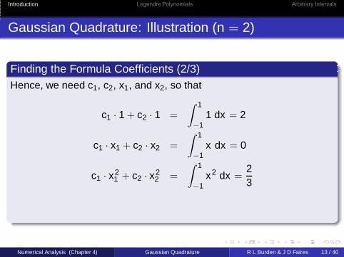
Finding the Formula Coefficients (2/3)Hence, we need c1, c2, x1, and x2, so that
c1 · 1 + c2 · 1 =
∫ 1
−11 dx = 2
c1 · x1 + c2 · x2 =
∫ 1
−1x dx = 0
c1 · x21 + c2 · x2
2 =
∫ 1
−1x2 dx =
23
Numerical Analysis (Chapter 4) Gaussian Quadrature R L Burden & J D Faires 13 / 40
Introduction Legendre Polynomials Arbitrary Intervals
Gaussian Quadrature: Illustration (n = 2)
Finding the Formula Coefficients (2/3)Hence, we need c1, c2, x1, and x2, so that
c1 · 1 + c2 · 1 =
∫ 1
−11 dx = 2
c1 · x1 + c2 · x2 =
∫ 1
−1x dx = 0
c1 · x21 + c2 · x2
2 =
∫ 1
−1x2 dx =
23
c1 · x31 + c2 · x3
2 =
∫ 1
−1x3 dx = 0
Numerical Analysis (Chapter 4) Gaussian Quadrature R L Burden & J D Faires 13 / 40
Introduction Legendre Polynomials Arbitrary Intervals
Gaussian Quadrature: Illustration (n = 2)
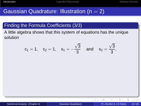
Finding the Formula Coefficients (3/3)A little algebra shows that this system of equations has the uniquesolution
c1 = 1, c2 = 1, x1 = −√
33
and x2 =
√3
3,
Numerical Analysis (Chapter 4) Gaussian Quadrature R L Burden & J D Faires 14 / 40
Introduction Legendre Polynomials Arbitrary Intervals
Gaussian Quadrature: Illustration (n = 2)
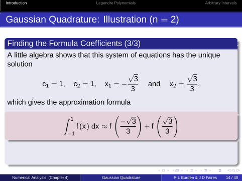
Finding the Formula Coefficients (3/3)A little algebra shows that this system of equations has the uniquesolution
c1 = 1, c2 = 1, x1 = −√
33
and x2 =
√3
3,
which gives the approximation formula
∫ 1
−1f (x) dx ≈ f
(
−√
33
)
+ f
(√3
3
)
Numerical Analysis (Chapter 4) Gaussian Quadrature R L Burden & J D Faires 14 / 40
Introduction Legendre Polynomials Arbitrary Intervals
Gaussian Quadrature: Illustration (n = 2)
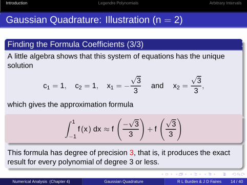
Finding the Formula Coefficients (3/3)A little algebra shows that this system of equations has the uniquesolution
c1 = 1, c2 = 1, x1 = −√
33
and x2 =
√3
3,
which gives the approximation formula
∫ 1
−1f (x) dx ≈ f
(
−√
33
)
+ f
(√3
3
)
This formula has degree of precision 3, that is, it produces the exactresult for every polynomial of degree 3 or less.
Numerical Analysis (Chapter 4) Gaussian Quadrature R L Burden & J D Faires 14 / 40
Introduction Legendre Polynomials Arbitrary Intervals
Outline
1 Gaussian Quadrature & Optimal Nodes
2 Using Legendre Polynomials to Derive Gaussian Quadrature Formulae
3 Gaussian Quadrature on Arbitrary Intervals
Numerical Analysis (Chapter 4) Gaussian Quadrature R L Burden & J D Faires 15 / 40
Introduction Legendre Polynomials Arbitrary Intervals
Gaussian Quadrature: Legendre Polynomials
An Alternative Method of Derivation
Numerical Analysis (Chapter 4) Gaussian Quadrature R L Burden & J D Faires 16 / 40
Introduction Legendre Polynomials Arbitrary Intervals
Gaussian Quadrature: Legendre Polynomials
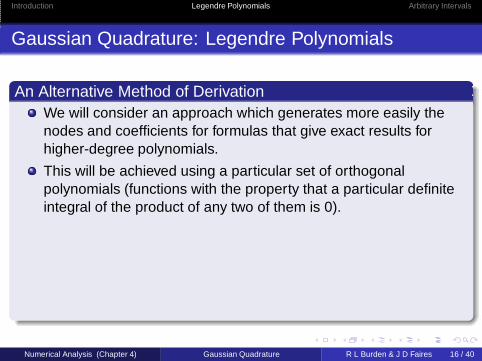
An Alternative Method of DerivationWe will consider an approach which generates more easily thenodes and coefficients for formulas that give exact results forhigher-degree polynomials.
Numerical Analysis (Chapter 4) Gaussian Quadrature R L Burden & J D Faires 16 / 40
Introduction Legendre Polynomials Arbitrary Intervals
Gaussian Quadrature: Legendre Polynomials
An Alternative Method of DerivationWe will consider an approach which generates more easily thenodes and coefficients for formulas that give exact results forhigher-degree polynomials.
This will be achieved using a particular set of orthogonalpolynomials (functions with the property that a particular definiteintegral of the product of any two of them is 0).
Numerical Analysis (Chapter 4) Gaussian Quadrature R L Burden & J D Faires 16 / 40
Introduction Legendre Polynomials Arbitrary Intervals
Gaussian Quadrature: Legendre Polynomials
An Alternative Method of DerivationWe will consider an approach which generates more easily thenodes and coefficients for formulas that give exact results forhigher-degree polynomials.
This will be achieved using a particular set of orthogonalpolynomials (functions with the property that a particular definiteintegral of the product of any two of them is 0).This set is the is the Legendre polynomials, a collection{P0(x), P1(x), . . . , Pn(x), . . . , } with properties:(1) For each n, Pn(x) is a monic polynomial of degree n.
(2)∫ 1
−1P(x)Pn(x) dx = 0 whenever P(x) is a polynomial of degree
less than n.
Numerical Analysis (Chapter 4) Gaussian Quadrature R L Burden & J D Faires 16 / 40
Introduction Legendre Polynomials Arbitrary Intervals
Gaussian Quadrature: Legendre Polynomials
Numerical Analysis (Chapter 4) Gaussian Quadrature R L Burden & J D Faires 17 / 40
Introduction Legendre Polynomials Arbitrary Intervals
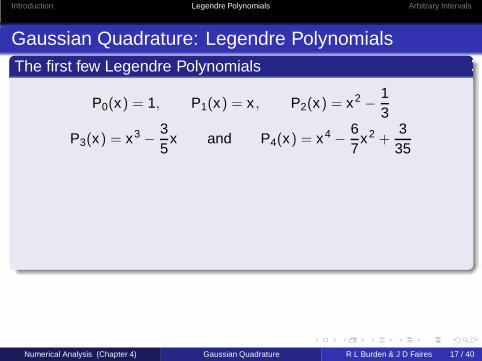
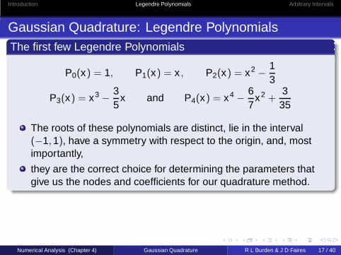
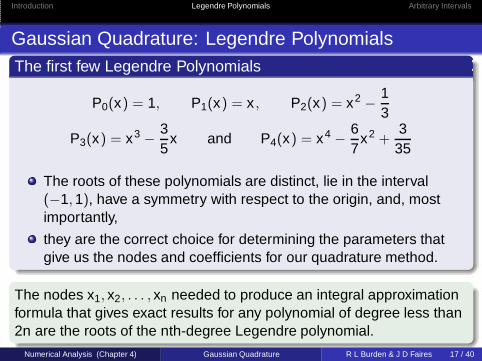
Gaussian Quadrature: Legendre PolynomialsThe first few Legendre Polynomials
P0(x) = 1, P1(x) = x , P2(x) = x2 − 13
P3(x) = x3 − 35
x and P4(x) = x4 − 67
x2 +3
35
Numerical Analysis (Chapter 4) Gaussian Quadrature R L Burden & J D Faires 17 / 40
Introduction Legendre Polynomials Arbitrary Intervals
Gaussian Quadrature: Legendre PolynomialsThe first few Legendre Polynomials
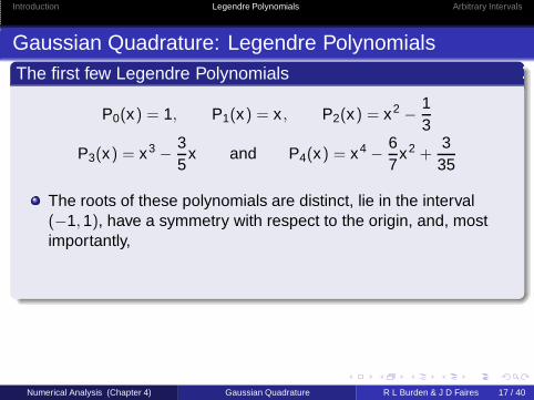
P0(x) = 1, P1(x) = x , P2(x) = x2 − 13
P3(x) = x3 − 35
x and P4(x) = x4 − 67
x2 +3
35
The roots of these polynomials are distinct, lie in the interval(−1, 1), have a symmetry with respect to the origin, and, mostimportantly,
Numerical Analysis (Chapter 4) Gaussian Quadrature R L Burden & J D Faires 17 / 40
Introduction Legendre Polynomials Arbitrary Intervals
Gaussian Quadrature: Legendre PolynomialsThe first few Legendre Polynomials
P0(x) = 1, P1(x) = x , P2(x) = x2 − 13
P3(x) = x3 − 35
x and P4(x) = x4 − 67
x2 +3
35
The roots of these polynomials are distinct, lie in the interval(−1, 1), have a symmetry with respect to the origin, and, mostimportantly,
they are the correct choice for determining the parameters thatgive us the nodes and coefficients for our quadrature method.
The nodes x1, x2, . . . , xn needed to produce an integral approximationformula that gives exact results for any polynomial of degree less than2n are the roots of the nth-degree Legendre polynomial.
Numerical Analysis (Chapter 4) Gaussian Quadrature R L Burden & J D Faires 17 / 40
Introduction Legendre Polynomials Arbitrary Intervals
Gaussian Quadrature: Legendre Polynomials
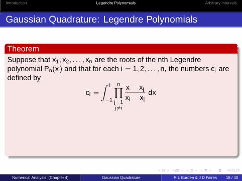
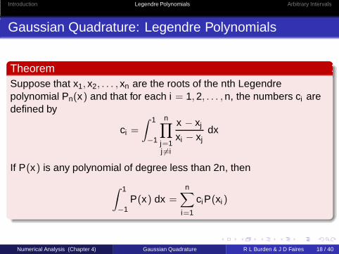
TheoremSuppose that x1, x2, . . . , xn are the roots of the nth Legendrepolynomial Pn(x) and that for each i = 1, 2, . . . , n, the numbers ci aredefined by
ci =
∫ 1
−1
n∏
j=1j 6=i
x − xj
xi − xjdx
Numerical Analysis (Chapter 4) Gaussian Quadrature R L Burden & J D Faires 18 / 40
Introduction Legendre Polynomials Arbitrary Intervals
Gaussian Quadrature: Legendre Polynomials
TheoremSuppose that x1, x2, . . . , xn are the roots of the nth Legendrepolynomial Pn(x) and that for each i = 1, 2, . . . , n, the numbers ci aredefined by
ci =
∫ 1
−1
n∏
j=1j 6=i
x − xj
xi − xjdx
If P(x) is any polynomial of degree less than 2n, then
∫ 1
−1P(x) dx =
n∑
i=1
ciP(xi )
Numerical Analysis (Chapter 4) Gaussian Quadrature R L Burden & J D Faires 18 / 40
Introduction Legendre Polynomials Arbitrary Intervals
Gaussian Quadrature: Legendre Polynomials
Proof (1/5)
Numerical Analysis (Chapter 4) Gaussian Quadrature R L Burden & J D Faires 19 / 40
Introduction Legendre Polynomials Arbitrary Intervals
Gaussian Quadrature: Legendre Polynomials
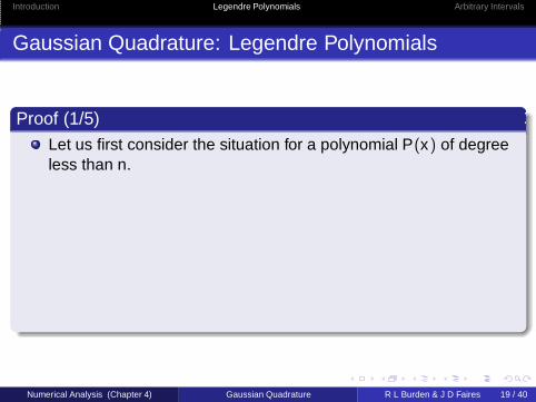
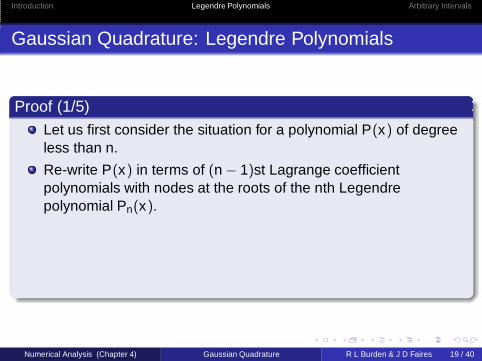
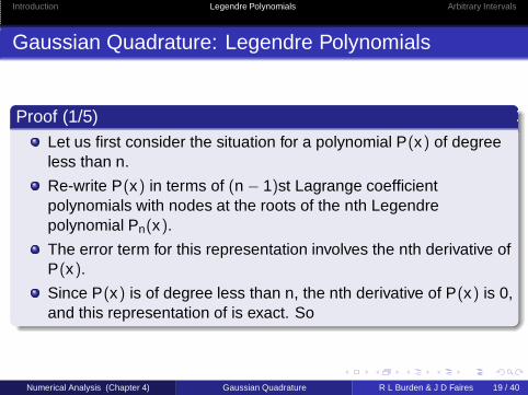
Proof (1/5)Let us first consider the situation for a polynomial P(x) of degreeless than n.
Numerical Analysis (Chapter 4) Gaussian Quadrature R L Burden & J D Faires 19 / 40
Introduction Legendre Polynomials Arbitrary Intervals
Gaussian Quadrature: Legendre Polynomials
Proof (1/5)Let us first consider the situation for a polynomial P(x) of degreeless than n.
Re-write P(x) in terms of (n − 1)st Lagrange coefficientpolynomials with nodes at the roots of the nth Legendrepolynomial Pn(x).
Numerical Analysis (Chapter 4) Gaussian Quadrature R L Burden & J D Faires 19 / 40

Introduction Legendre Polynomials Arbitrary Intervals
Gaussian Quadrature: Legendre Polynomials
Proof (1/5)Let us first consider the situation for a polynomial P(x) of degreeless than n.
Re-write P(x) in terms of (n − 1)st Lagrange coefficientpolynomials with nodes at the roots of the nth Legendrepolynomial Pn(x).
The error term for this representation involves the nth derivative ofP(x).
Numerical Analysis (Chapter 4) Gaussian Quadrature R L Burden & J D Faires 19 / 40
Introduction Legendre Polynomials Arbitrary Intervals
Gaussian Quadrature: Legendre Polynomials
Proof (1/5)Let us first consider the situation for a polynomial P(x) of degreeless than n.
Re-write P(x) in terms of (n − 1)st Lagrange coefficientpolynomials with nodes at the roots of the nth Legendrepolynomial Pn(x).
The error term for this representation involves the nth derivative ofP(x).
Since P(x) is of degree less than n, the nth derivative of P(x) is 0,and this representation of is exact. So
Numerical Analysis (Chapter 4) Gaussian Quadrature R L Burden & J D Faires 19 / 40
Introduction Legendre Polynomials Arbitrary Intervals
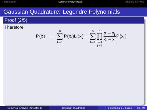
Gaussian Quadrature: Legendre PolynomialsProof (2/5)
Numerical Analysis (Chapter 4) Gaussian Quadrature R L Burden & J D Faires 20 / 40
Introduction Legendre Polynomials Arbitrary Intervals
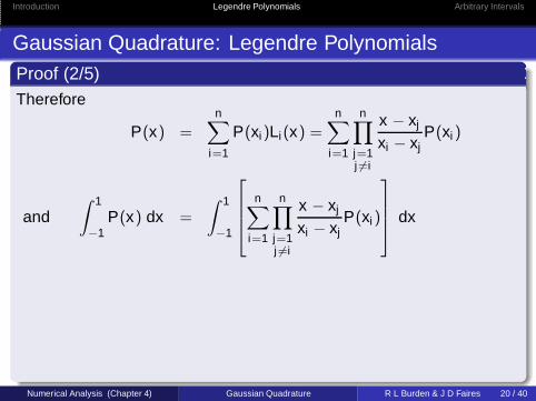
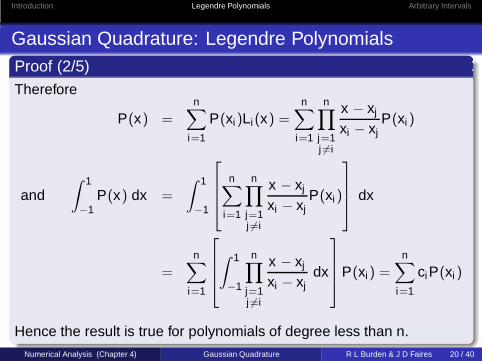
Gaussian Quadrature: Legendre PolynomialsProof (2/5)Therefore
P(x) =n∑
i=1
P(xi)Li(x) =n∑
i=1
n∏
j=1j 6=i
x − xj
xi − xjP(xi )
Numerical Analysis (Chapter 4) Gaussian Quadrature R L Burden & J D Faires 20 / 40
Introduction Legendre Polynomials Arbitrary Intervals
Gaussian Quadrature: Legendre PolynomialsProof (2/5)Therefore
P(x) =n∑
i=1
P(xi)Li(x) =n∑
i=1
n∏
j=1j 6=i
x − xj
xi − xjP(xi )
and∫ 1
−1P(x) dx =
∫ 1
−1
n∑
i=1
n∏
j=1j 6=i
x − xj
xi − xjP(xi )
dx
=n∑
i=1
∫ 1
−1
n∏
j=1j 6=i
x − xj
xi − xjdx
P(xi) =n∑
i=1
ciP(xi )
Hence the result is true for polynomials of degree less than n.Numerical Analysis (Chapter 4) Gaussian Quadrature R L Burden & J D Faires 20 / 40
Introduction Legendre Polynomials Arbitrary Intervals
Gaussian Quadrature: Legendre Polynomials
Proof (3/5)
Numerical Analysis (Chapter 4) Gaussian Quadrature R L Burden & J D Faires 21 / 40
Introduction Legendre Polynomials Arbitrary Intervals
Gaussian Quadrature: Legendre Polynomials
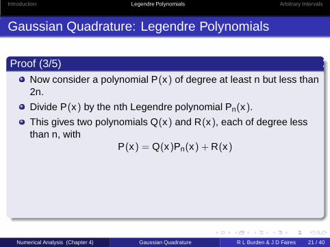
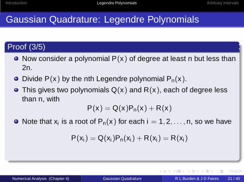
Proof (3/5)Now consider a polynomial P(x) of degree at least n but less than2n.
Numerical Analysis (Chapter 4) Gaussian Quadrature R L Burden & J D Faires 21 / 40
Introduction Legendre Polynomials Arbitrary Intervals
Gaussian Quadrature: Legendre Polynomials
Proof (3/5)Now consider a polynomial P(x) of degree at least n but less than2n.
Divide P(x) by the nth Legendre polynomial Pn(x).
This gives two polynomials Q(x) and R(x), each of degree lessthan n, with
P(x) = Q(x)Pn(x) + R(x)
Note that xi is a root of Pn(x) for each i = 1, 2, . . . , n, so we have
P(xi ) = Q(xi )Pn(xi) + R(xi) = R(xi)
We now invoke the unique power of the Legendre polynomials.
Numerical Analysis (Chapter 4) Gaussian Quadrature R L Burden & J D Faires 21 / 40
Introduction Legendre Polynomials Arbitrary Intervals
Gaussian Quadrature: Legendre Polynomials
Proof (4/5)
Numerical Analysis (Chapter 4) Gaussian Quadrature R L Burden & J D Faires 22 / 40
Introduction Legendre Polynomials Arbitrary Intervals
Gaussian Quadrature: Legendre Polynomials
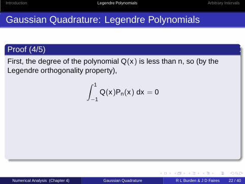
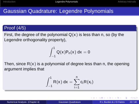
Proof (4/5)First, the degree of the polynomial Q(x) is less than n, so (by theLegendre orthogonality property),
∫ 1
−1Q(x)Pn(x) dx = 0
Numerical Analysis (Chapter 4) Gaussian Quadrature R L Burden & J D Faires 22 / 40
Introduction Legendre Polynomials Arbitrary Intervals
Gaussian Quadrature: Legendre Polynomials
Proof (4/5)First, the degree of the polynomial Q(x) is less than n, so (by theLegendre orthogonality property),
∫ 1
−1Q(x)Pn(x) dx = 0
Then, since R(x) is a polynomial of degree less than n, the openingargument implies that
∫ 1
−1R(x) dx =
n∑
i=1
ciR(xi)
Numerical Analysis (Chapter 4) Gaussian Quadrature R L Burden & J D Faires 22 / 40
Introduction Legendre Polynomials Arbitrary Intervals
Gaussian Quadrature: Legendre Polynomials
Proof (5/5)
Numerical Analysis (Chapter 4) Gaussian Quadrature R L Burden & J D Faires 23 / 40
Introduction Legendre Polynomials Arbitrary Intervals
Gaussian Quadrature: Legendre Polynomials
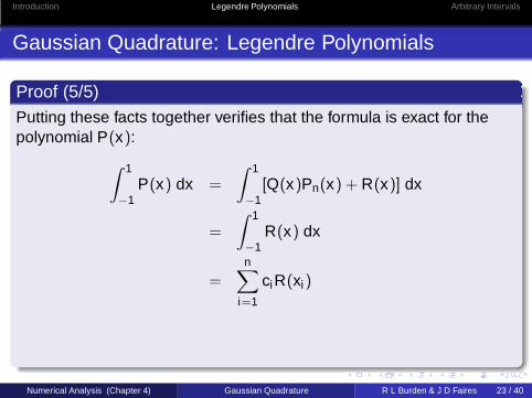
Proof (5/5)Putting these facts together verifies that the formula is exact for thepolynomial P(x):
Numerical Analysis (Chapter 4) Gaussian Quadrature R L Burden & J D Faires 23 / 40

Introduction Legendre Polynomials Arbitrary Intervals
Gaussian Quadrature: Legendre Polynomials
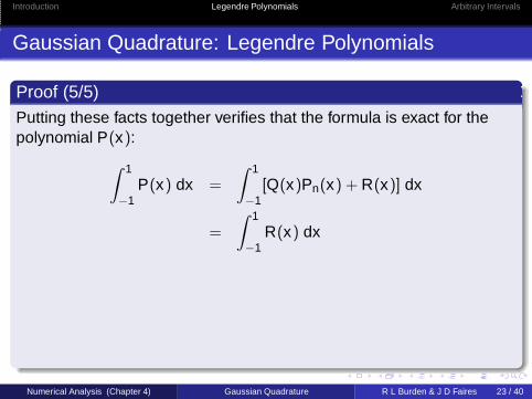
Proof (5/5)Putting these facts together verifies that the formula is exact for thepolynomial P(x):
∫ 1
−1P(x) dx =
∫ 1
−1[Q(x)Pn(x) + R(x)] dx
Numerical Analysis (Chapter 4) Gaussian Quadrature R L Burden & J D Faires 23 / 40
Introduction Legendre Polynomials Arbitrary Intervals
Gaussian Quadrature: Legendre Polynomials
Proof (5/5)Putting these facts together verifies that the formula is exact for thepolynomial P(x):
∫ 1
−1P(x) dx =
∫ 1
−1[Q(x)Pn(x) + R(x)] dx
=
∫ 1
−1R(x) dx
=n∑
i=1
ciR(xi)
Numerical Analysis (Chapter 4) Gaussian Quadrature R L Burden & J D Faires 23 / 40

Introduction Legendre Polynomials Arbitrary Intervals
Gaussian Quadrature: Legendre Polynomials
Proof (5/5)Putting these facts together verifies that the formula is exact for thepolynomial P(x):
∫ 1
−1P(x) dx =
∫ 1
−1[Q(x)Pn(x) + R(x)] dx
=
∫ 1
−1R(x) dx
=n∑
i=1
ciR(xi)
=n∑
i=1
ciP(xi)
Numerical Analysis (Chapter 4) Gaussian Quadrature R L Burden & J D Faires 23 / 40
Introduction Legendre Polynomials Arbitrary Intervals
Gaussian Quadrature: Roots & Coefficients
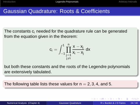
The constants ci needed for the quadrature rule can be generatedfrom the equation given in the theorem:
ci =
∫ 1
−1
n∏
j=1j 6=i
x − xj
xi − xjdx
but both these constants and the roots of the Legendre polynomialsare extensively tabulated.
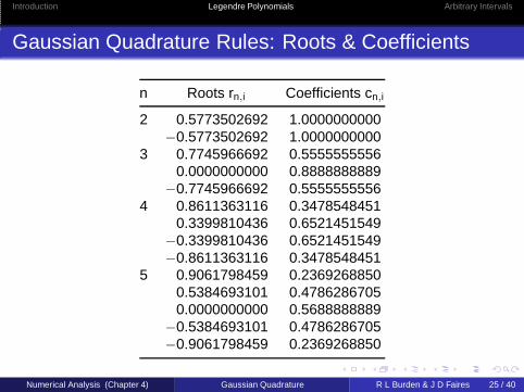
The following table lists these values for n = 2, 3, 4, and 5.
Numerical Analysis (Chapter 4) Gaussian Quadrature R L Burden & J D Faires 24 / 40
Introduction Legendre Polynomials Arbitrary Intervals
Gaussian Quadrature Rules: Roots & Coefficients
n Roots rn,i Coefficients cn,i
2 0.5773502692 1.0000000000−0.5773502692 1.0000000000
3 0.7745966692 0.55555555560.0000000000 0.8888888889
−0.7745966692 0.55555555564 0.8611363116 0.3478548451
0.3399810436 0.6521451549−0.3399810436 0.6521451549−0.8611363116 0.3478548451
5 0.9061798459 0.23692688500.5384693101 0.47862867050.0000000000 0.5688888889
−0.5384693101 0.4786286705−0.9061798459 0.2369268850
Numerical Analysis (Chapter 4) Gaussian Quadrature R L Burden & J D Faires 25 / 40
Introduction Legendre Polynomials Arbitrary Intervals
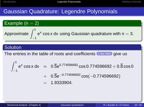
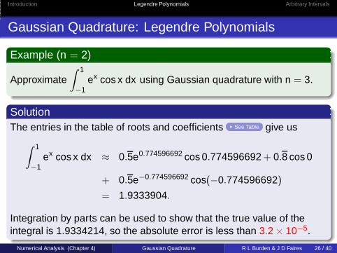
Gaussian Quadrature: Legendre Polynomials
Example (n = 2)
Approximate∫ 1
−1ex cos x dx using Gaussian quadrature with n = 3.
SolutionThe entries in the table of roots and coefficients See Table
Numerical Analysis (Chapter 4) Gaussian Quadrature R L Burden & J D Faires 26 / 40
Introduction Legendre Polynomials Arbitrary Intervals
Gaussian Quadrature: Legendre Polynomials
Example (n = 2)
Approximate∫ 1
−1ex cos x dx using Gaussian quadrature with n = 3.
SolutionThe entries in the table of roots and coefficients See Table give us
∫ 1
−1ex cos x dx ≈ 0.5e0.774596692 cos 0.774596692 + 0.8 cos 0
+ 0.5e−0.774596692 cos(−0.774596692)
= 1.9333904.
Integration by parts can be used to show that the true value of theintegral is 1.9334214, so the absolute error is less than 3.2 × 10⁻⁵.
Numerical Analysis (Chapter 4) Gaussian Quadrature R L Burden & J D Faires 26 / 40
Introduction Legendre Polynomials Arbitrary Intervals
Outline
1 Gaussian Quadrature & Optimal Nodes
2 Using Legendre Polynomials to Derive Gaussian Quadrature Formulae
3 Gaussian Quadrature on Arbitrary Intervals
Numerical Analysis (Chapter 4) Gaussian Quadrature R L Burden & J D Faires 27 / 40
Introduction Legendre Polynomials Arbitrary Intervals
Gaussian Quadrature on Arbitrary Intervals
Transform the Interval of Integration to [−1, 1]
An integral∫ b
a f (x) dx over an arbitrary [a, b] can be transformed intoan integral over [−1, 1] by using the change of variables See Diagram :
t =2x − a − b
b − a⇐⇒ x =
12
[(b − a)t + a + b]
Numerical Analysis (Chapter 4) Gaussian Quadrature R L Burden & J D Faires 28 / 40
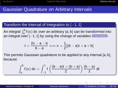
Introduction Legendre Polynomials Arbitrary Intervals
Gaussian Quadrature on Arbitrary Intervals
Transform the Interval of Integration to [−1, 1]
An integral∫ b
a f (x) dx over an arbitrary [a, b] can be transformed intoan integral over [−1, 1] by using the change of variables See Diagram :
t =2x − a − b
b − a⇐⇒ x =
12
[(b − a)t + a + b]
This permits Gaussian quadrature to be applied to any interval [a, b],because
∫ b
af (x) dx =
∫ 1
−1f(
(b − a)t + (b + a)
2
)
(b − a)
2dt
Numerical Analysis (Chapter 4) Gaussian Quadrature R L Burden & J D Faires 28 / 40
Introduction Legendre Polynomials Arbitrary Intervals
Gaussian Quadrature on Arbitrary Intervals
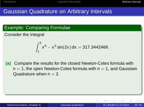
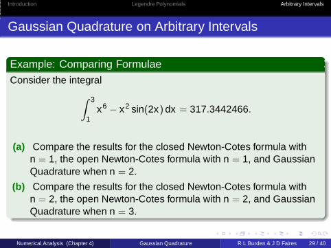
Example: Comparing FormulaeConsider the integral
∫ 3
1x6 − x2 sin(2x) dx = 317.3442466.
Numerical Analysis (Chapter 4) Gaussian Quadrature R L Burden & J D Faires 29 / 40
Introduction Legendre Polynomials Arbitrary Intervals
Gaussian Quadrature on Arbitrary Intervals
Example: Comparing FormulaeConsider the integral
∫ 3
1x6 − x2 sin(2x) dx = 317.3442466.
(a) Compare the results for the closed Newton-Cotes formula withn = 1, the open Newton-Cotes formula with n = 1, and GaussianQuadrature when n = 2.
(b) Compare the results for the closed Newton-Cotes formula withn = 2, the open Newton-Cotes formula with n = 2, and GaussianQuadrature when n = 3.
Numerical Analysis (Chapter 4) Gaussian Quadrature R L Burden & J D Faires 29 / 40
Introduction Legendre Polynomials Arbitrary Intervals
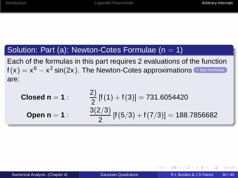
Solution: Part (a): Newton-Cotes Formulae (n = 1)Each of the formulas in this part requires 2 evaluations of the functionf (x) = x6 − x2 sin(2x). The Newton-Cotes approximations See Formulae
are:
Closed n = 1 :2)
2[f (1) + f (3)] = 731.6054420
Open n = 1 :3(2/3)
2[f (5/3) + f (7/3)] = 188.7856682
Numerical Analysis (Chapter 4) Gaussian Quadrature R L Burden & J D Faires 30 / 40
Introduction Legendre Polynomials Arbitrary Intervals
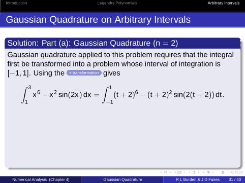
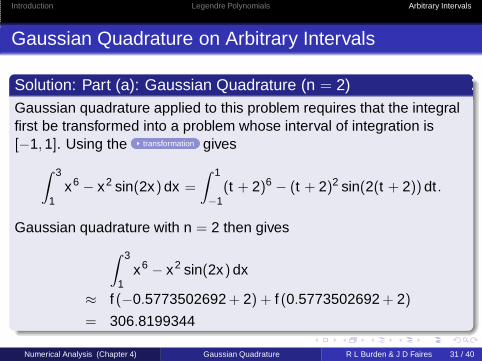
Gaussian Quadrature on Arbitrary Intervals
Solution: Part (a): Gaussian Quadrature (n = 2)Gaussian quadrature applied to this problem requires that the integralfirst be transformed into a problem whose interval of integration is[−1, 1]. Using the transformation gives
∫ 3
1x6 − x2 sin(2x) dx =
∫ 1
−1(t + 2)6 − (t + 2)2 sin(2(t + 2)) dt .
Numerical Analysis (Chapter 4) Gaussian Quadrature R L Burden & J D Faires 31 / 40
Introduction Legendre Polynomials Arbitrary Intervals
Gaussian Quadrature on Arbitrary Intervals
Solution: Part (a): Gaussian Quadrature (n = 2)Gaussian quadrature applied to this problem requires that the integralfirst be transformed into a problem whose interval of integration is[−1, 1]. Using the transformation gives
∫ 3
1x6 − x2 sin(2x) dx =
∫ 1
−1(t + 2)6 − (t + 2)2 sin(2(t + 2)) dt .
Gaussian quadrature with n = 2 then gives
∫ 3
1x6 − x2 sin(2x) dx
≈ f (−0.5773502692 + 2) + f (0.5773502692 + 2)
= 306.8199344
Numerical Analysis (Chapter 4) Gaussian Quadrature R L Burden & J D Faires 31 / 40
Introduction Legendre Polynomials Arbitrary Intervals
Gaussian Quadrature on Arbitrary Intervals
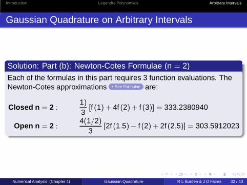
Solution: Part (b): Newton-Cotes Formulae (n = 2)Each of the formulas in this part requires 3 function evaluations. TheNewton-Cotes approximations See Formulae are:
Closed n = 2 :1)
3[f (1) + 4f (2) + f (3)] = 333.2380940
Open n = 2 :4(1/2)
3[2f (1.5)− f (2) + 2f (2.5)] = 303.5912023
Numerical Analysis (Chapter 4) Gaussian Quadrature R L Burden & J D Faires 32 / 40
Introduction Legendre Polynomials Arbitrary Intervals
Gaussian Quadrature on Arbitrary Intervals
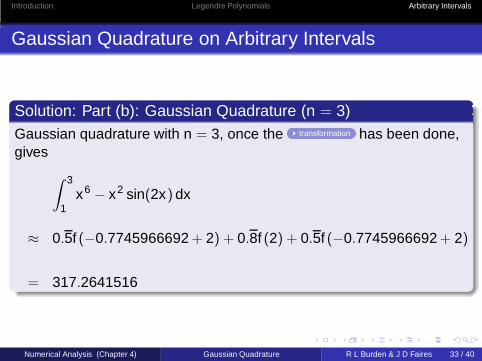
Solution: Part (b): Gaussian Quadrature (n = 3)Gaussian quadrature with n = 3, once the transformation has been done,gives
∫ 3
1x6 − x2 sin(2x) dx
≈ 0.5f (−0.7745966692 + 2) + 0.8f (2) + 0.5f (−0.7745966692 + 2)
= 317.2641516
Numerical Analysis (Chapter 4) Gaussian Quadrature R L Burden & J D Faires 33 / 40

Introduction Legendre Polynomials Arbitrary Intervals
Gaussian Quadrature on Arbitrary Intervals
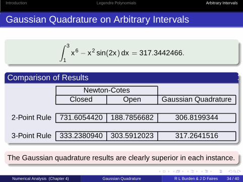
∫ 3
1x6 − x2 sin(2x) dx = 317.3442466.
Numerical Analysis (Chapter 4) Gaussian Quadrature R L Burden & J D Faires 34 / 40
Introduction Legendre Polynomials Arbitrary Intervals
Gaussian Quadrature on Arbitrary Intervals
∫ 3
1x6 − x2 sin(2x) dx = 317.3442466.
Comparison of Results
Newton-CotesClosed Open Gaussian Quadrature
2-Point Rule 731.6054420 188.7856682 306.8199344
3-Point Rule 333.2380940 303.5912023 317.2641516
The Gaussian quadrature results are clearly superior in each instance.
Numerical Analysis (Chapter 4) Gaussian Quadrature R L Burden & J D Faires 34 / 40

Questions?

Reference Material
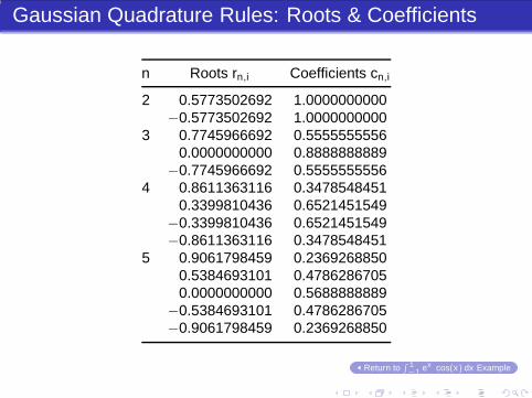
Gaussian Quadrature Rules: Roots & Coefficients
n Roots rn,i Coefficients cn,i
2 0.5773502692 1.0000000000−0.5773502692 1.0000000000
3 0.7745966692 0.55555555560.0000000000 0.8888888889
−0.7745966692 0.55555555564 0.8611363116 0.3478548451
0.3399810436 0.6521451549−0.3399810436 0.6521451549−0.8611363116 0.3478548451
5 0.9061798459 0.23692688500.5384693101 0.47862867050.0000000000 0.5688888889
−0.5384693101 0.4786286705−0.9061798459 0.2369268850
Return to∫ 1−1 ex cos(x) dx Example
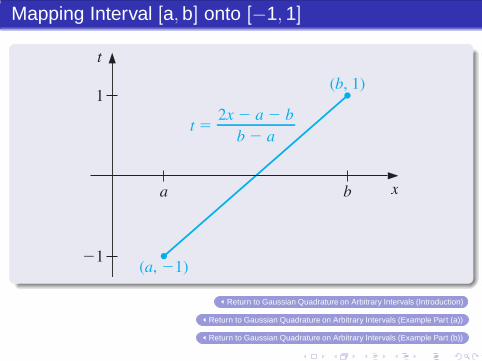
Mapping Interval [a, b] onto [−1, 1]
t
x
21
1
a b
(a, 21)
(b, 1)
2x 2 a 2 bt 5
b 2 a
Return to Gaussian Quadrature on Arbitrary Intervals (Introduction)
Return to Gaussian Quadrature on Arbitrary Intervals (Example Part (a))
Return to Gaussian Quadrature on Arbitrary Intervals (Example Part (b))
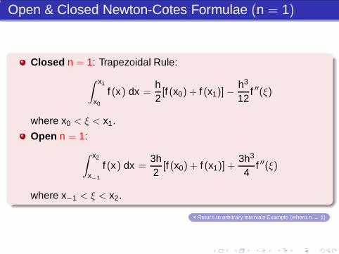
Open & Closed Newton-Cotes Formulae (n = 1)
Closed n = 1: Trapezoidal Rule:
∫ x1
x0
f (x) dx =h2
[f (x0) + f (x1)] −h3
12f ′′(ξ)
where x0 < ξ < x1.
Open n = 1:
∫ x2
x−1
f (x) dx =3h2
[f (x0) + f (x1)] +3h3
4f ′′(ξ)
where x−1 < ξ < x2.
Return to arbitrary intervals Example (where n = 1)
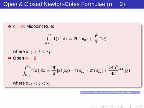
Open & Closed Newton-Cotes Formulae (n = 2)
n = 0: Midpoint Rule:
∫ x1
x−1
f (x) dx = 2hf (x0) +h3
3f ′′(ξ)
where x−1 < ξ < x1.
Open n = 2
∫ x3
x−1
f (x) dx =4h3
[2f (x0) − f (x1) + 2f (x2)] +14h5
45f (4)(ξ)
where x−1 < ξ < x3.
Return to arbitrary intervals Example (where n = 1)


![Numerical Differentiation & Integration [0.125in]3.375in0 ...mamu/courses/231/Slides/CH04_1A.pdf · Numerical Differentiation Example 1: f(x) = lnx Use the forward-difference formula](https://img.pdfslide.us/doc/110x75/5e47b0181514ed75101685ff/numerical-differentiation-integration-0125in3375in0-mamucourses231slidesch041apdf.jpg)
![Numerical Differentiation & Integration [0.125in]3.375in0 ...mamu/courses/231/Slides/CH04_4A.pdf · Numerical Differentiation & Integration Composite Numerical Integration I Numerical](https://img.pdfslide.us/doc/110x75/5b1fb63d7f8b9a112c8b4a5d/numerical-differentiation-integration-0125in3375in0-mamucourses231slidesch044apdf.jpg)

![Numerical Differentiation & Integration [0.125in]3.375in0 ...mamu/courses/231/Slides/CH04_1B.pdf · Numerical Analysis (Chapter 4) Numerical Differentiation II R L Burden & J D Faires](https://img.pdfslide.us/doc/110x75/5ebb51c88a3e5e19b4639f16/numerical-differentiation-integration-0125in3375in0-mamucourses231slidesch041bpdf.jpg)

![Numerical Differentiation & Integration [0.125in]3.375in0](https://img.pdfslide.us/doc/110x75/616a2ae511a7b741a34f8ac6/numerical-differentiation-amp-integration-0125in3375in0-.jpg)