Creating the Calibration Curve and Generating Method 8261 Quantitation Reports through

SMCReporter V4.0

Michael H. Hiatt U.S. Environmental Protection Agency

National Exposure Research Laboratory Environmental Sciences Division

P.O. Box 93478, Las Vegas, Nevada 89193-3478

Demonstration. Install SMCREPORTER

• This slide show is in addition to documentation provided with method 8261 software.

• The reader can reproduce the processing to be presented by installing Smcreporter 4.0 http://www.epa.gov/nerlesd1/chemistry/vacuu m/methods/software.htm

• Download the zip file as per Installation Guide at the site.

• You will have created a folder “SMCREPORTER” on the C drive as the default.

Load Demonstration Files for this Exercise

• The reader can reproduce the processing to be presented by installing data files used. They can be downloaded in a zip file (example.zip) from http://www.epa.gov/nerlesd1/chemistry/vacuum/methods/software. htm

• When the software and data files are installed, a new folder, SMCREPORTER, is created. Under this folder a sub-folder, Example, contains the example data files including the method 8261 library (CLPLibrary.txt), internal standard file (CLP

• istds.ini), blank (t4050601.txt), and five standards (t4050604.txt , t4050605.txt , t4050606.txt , t4050607.txt , t4050609.txt).

• This presentation assumes an understanding of the method 8261 calculations using surrogates. See http://www.epa.gov/nerlesd1/chemistry/vacuum/reference/analysis /anal.htm .

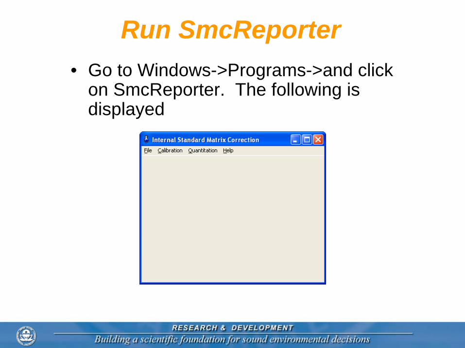
Run SmcReporter• Go to Windows->Programs->and click

on SmcReporter. The following is displayed

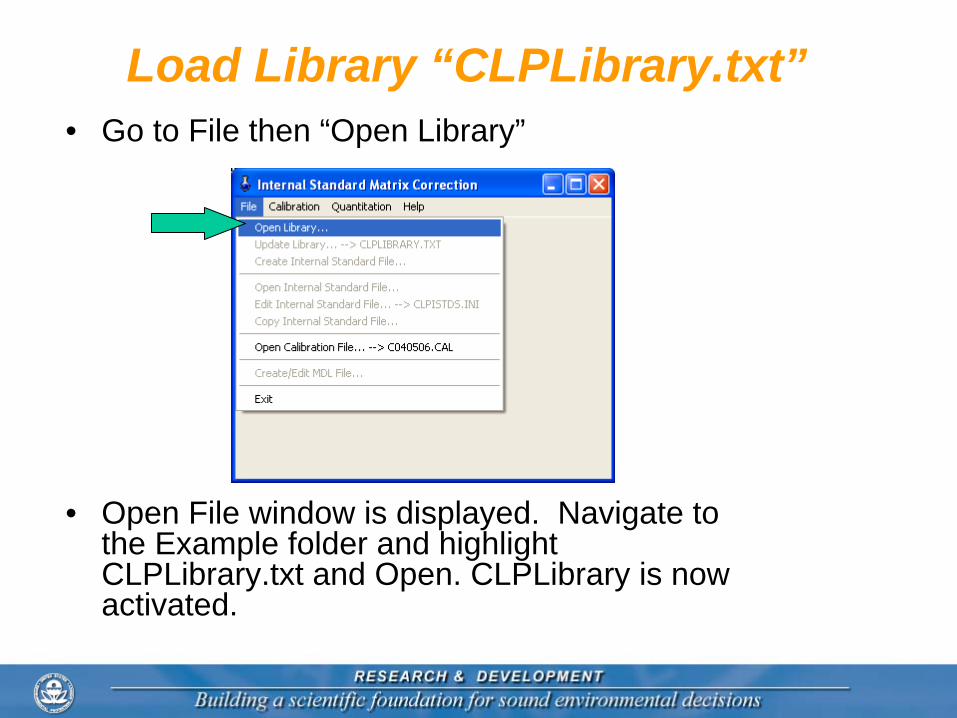
Load Library “CLPLibrary.txt”• Go to File then “Open Library”

• Open File window is displayed. Navigate to the Example folder and highlight CLPLibrary.txt and Open. CLPLibrary is now activated.

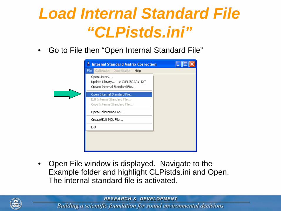
Load Internal Standard File “CLPistds.ini”

• Go to File then “Open Internal Standard File”

• Open File window is displayed. Navigate to the Example folder and highlight CLPistds.ini and Open. The internal standard file is activated.

GC/MS data set

• The raw data must be in ASCII format and readable in Notepad (e.g. t4050601.txt)

• These text files are generated by software available on this site and convert instrument data files to the required format.

• These data files contain the GC/MS response (area) and retention time for each compound.

• Each compound in the “CLPlibrary.txt” library is present in the data file.

• The first line of the data file contains the label “DATA FILE” followed by version of software

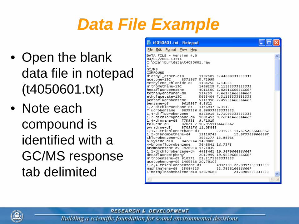
Data File Example

• Open the blank data file in notepad (t4050601.txt)

• Note each compound is identified with a GC/MS response tab delimited

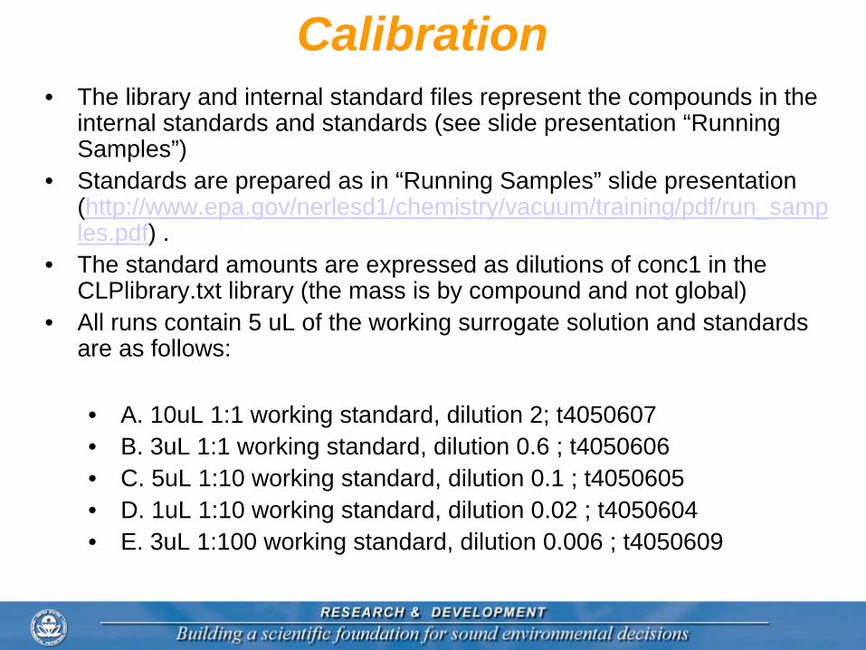
Calibration• The library and internal standard files represent the compounds in the

internal standards and standards (see slide presentation “Running Samples”)

• Standards are prepared as in “Running Samples” slide presentation (http://www.epa.gov/nerlesd1/chemistry/vacuum/training/pdf/run_samp les.pdf) .

• The standard amounts are expressed as dilutions of conc1 in the CLPlibrary.txt library (the mass is by compound and not global)

• All runs contain 5 uL of the working surrogate solution and standards are as follows:

• A. 10uL 1:1 working standard, dilution 2; t4050607• B. 3uL 1:1 working standard, dilution 0.6 ; t4050606• C. 5uL 1:10 working standard, dilution 0.1 ; t4050605• D. 1uL 1:10 working standard, dilution 0.02 ; t4050604• E. 3uL 1:100 working standard, dilution 0.006 ; t4050609

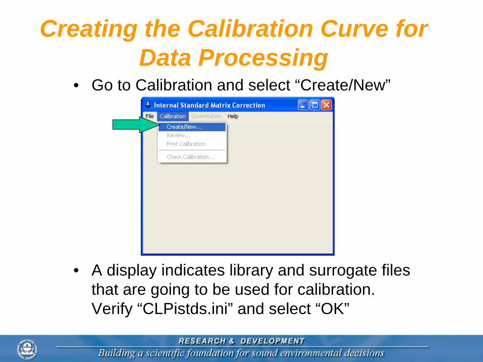
Creating the Calibration Curve for Data Processing

• Go to Calibration and select “Create/New”

• A display indicates library and surrogate files that are going to be used for calibration. Verify “CLPistds.ini” and select “OK”

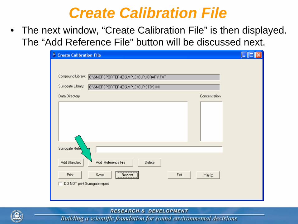
Create Calibration File • The next window, “Create Calibration File” is then displayed.

The “Add Reference File” button will be discussed next.

Reference File• The reference file used in calibration is the initial condition of

internal standards that the standard are compared. The response of internal standard compounds in the reference file is taken to be the 100 % response. The internal standards in the standard runs are compared to their response in the reference file and deviations from 100% are determined as functions of their boiling points (BP’s) and relative volatilities ("’s).

• An internal standard reference file can be any of the runs used to generate a calibration but typically, the blank run (t4050601.txt) run prior to the calibration standards is used.

• Select “Add Reference File” and using the “Open” window that is displayed navigate to the Example folder and select the t4050601.txt file.

• Internal standards have been called ‘surrogates” in the past (and you will still see some use of ‘surrogates’ in place of internal standards.

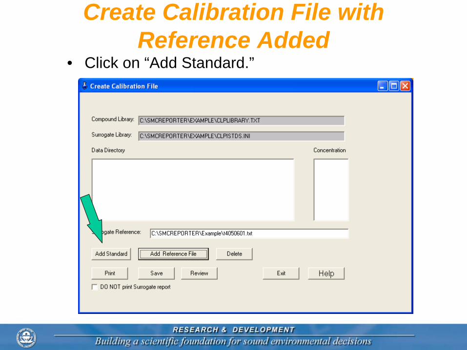
Create Calibration File with Reference Added

• Click on “Add Standard.”

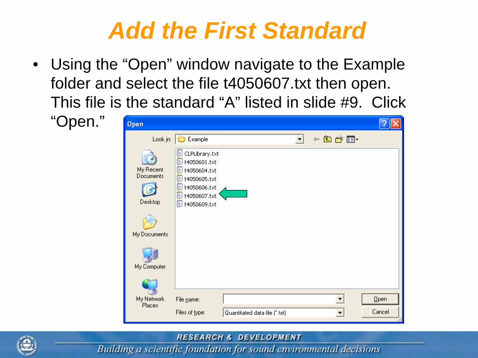
Add the First Standard• Using the “Open” window navigate to the Example

folder and select the file t4050607.txt then open. This file is the standard “A” listed in slide #9. Click “Open.”

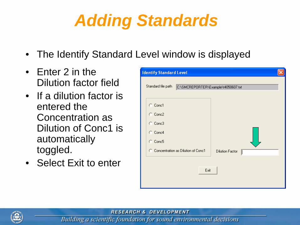
Adding Standards

• The Identify Standard Level window is displayed

• Enter 2 in the Dilution factor field

• If a dilution factor is entered the Concentration as Dilution of Conc1 is automatically toggled.

• Select Exit to enter

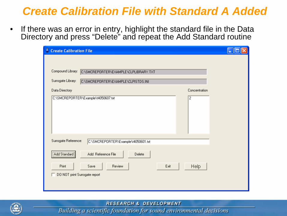
Create Calibration File with Standard A Added• If there was an error in entry, highlight the standard file in the Data

Directory and press “Delete” and repeat the Add Standard routine

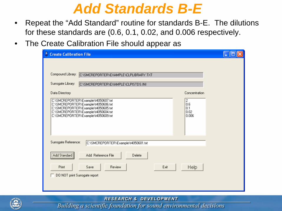
Add Standards B-E• Repeat the “Add Standard” routine for standards B-E. The dilutions

for these standards are (0.6, 0.1, 0.02, and 0.006 respectively.• The Create Calibration File should appear as

Review calibration curve• If all entries are correct the next step is to review

the data.• Press the “Review” tab on the “Create

Calibration File” form.• The following slide presents the “Review

Calibration” form, starting at the first library entry ( the default).

• Note that no sample sizes are entered. Only the total ngs are being displayed. This is an important feature of method 8261 as calibration is by mass and not by matrix or sample size.

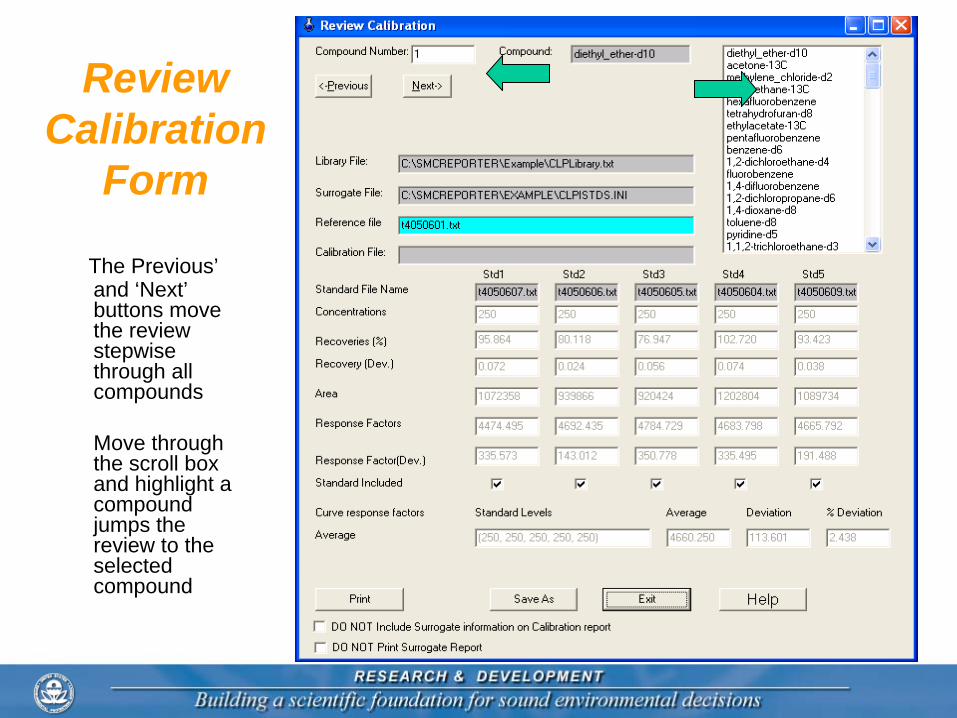
Review Calibration

Form

The Previous’ and ‘Next’ buttons move the review stepwise through all compounds

Move through the scroll box and highlight a compound jumps the review to the selected compound

Reviewing Calibration by Compound

• By selecting the “Next” tab (upper left corner) each compound is displayed.

• Scroll or jump the review to chloroethane. If you scroll you will see the % Deviation box (toward lower left) of all compounds have been <25 % until we get to chloroethane.

• The results for chloroethane show that the lowest standard (1.5ng) response factor is not equivalent to the others.

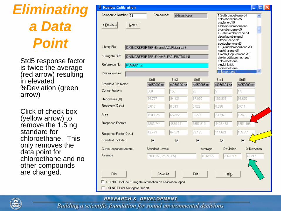
Eliminating a Data Point

Std5 response factor is twice the average (red arrow) resulting in elevated %Deviation (green arrow)

Click of check box (yellow arrow) to remove the 1.5 ng standard for chloroethane. This only removes the data point for chloroethane and no other compounds are changed.

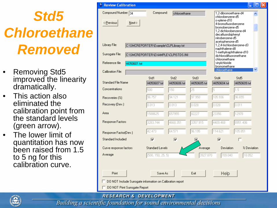
Std5 Chloroethane

Removed• Removing Std5

improved the linearity dramatically.

• This action also eliminated the calibration point from the standard levels (green arrow).

• The lower limit of quantitation has now been raised from 1.5 to 5 ng for this calibration curve.

Editing the Calibration Curve• The large deviation for chloroethane indicated there was a

problem with the compound at the lowest concentration.• Evaluating the chromatogram for chloroethane we found that

low level interference was causing the bias. • Removing a calibration point for a compound changes the

calibration range. Such changes may be necessary to ensure the response factor is consistent and we are working a justifiable calibration range.

• When compounds are also consistently in the system blanks their low calibration points could be compromised and these should also be ‘unchecked’. This action puts background below LOQ and also mitigates background bias from their response factor.

• By removing a data point, the linearity will be recalculated and the LOQ changed.

More Changes!• Stepping through the calibration review we find diethyl ether

(compound #36) is the next compound that requires the low-level calibration point to be removed.

• The next compound that has a large linearity deviation is a common laboratory contaminant, Acetone (#38). This compound is a very persistent compound in the laboratory that generated the data as the laboratory is not isolated as most volatile analyses laboratories. Removing all data points except the largest raises the LOQ to the highest standard. This means any detection of acetone in a sample will be flagged as below LOQ or exceeds the upper limit of quantitation.

• Methylene chloride (#45) and 2-butanone are additional laboratory contaminants and their two lowest calibration points are unchecked.

• If a compound is not detected in a standard, the standard included checkbox is unchecked and the calibration point is not used in the calibration range.

• Additional compounds that are to be unchecked from the lowest standard are 39, 43, 54, 61, 69, 73, 112, 114, and 115.

Save calibration curve• After the review, save the calibration curve.

Click on the “Save as” button on the lower right hand corner of the review and save the file as “Calibration.cal”.

• The calibration file is a standalone file containing all information necessary to process sample data. If the SMCReporter program is closed test.cal can be reloaded for sample processing. “CLPlibrary.txt” and “CLPistds.ini” do not have to be recalled.

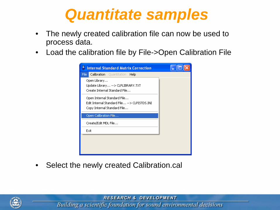
Quantitate samples• The newly created calibration file can now be used to

process data.• Load the calibration file by File->Open Calibration File

• Select the newly created Calibration.cal

Calibration Loaded

• Notice that after loading the calibration file that library CLPlibrary.txt and CLPistds.ini are disabled (under File).

• The main window (see slide 4) now has Calibration and Quantitation menu options enabled.

• In the Calibration menu options for review, printing, and check standard reporting are now enabled.

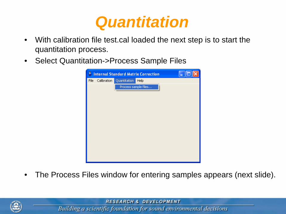
Quantitation• With calibration file test.cal loaded the next step is to start the

quantitation process.• Select Quantitation->Process Sample Files

• The Process Files window for entering samples appears (next slide).

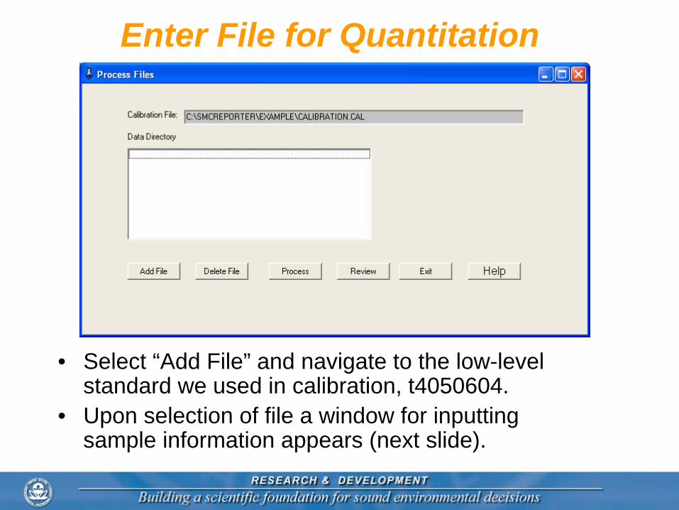
Enter File for Quantitation

• Select “Add File” and navigate to the low-level standard we used in calibration, t4050604.

• Upon selection of file a window for inputting sample information appears (next slide).

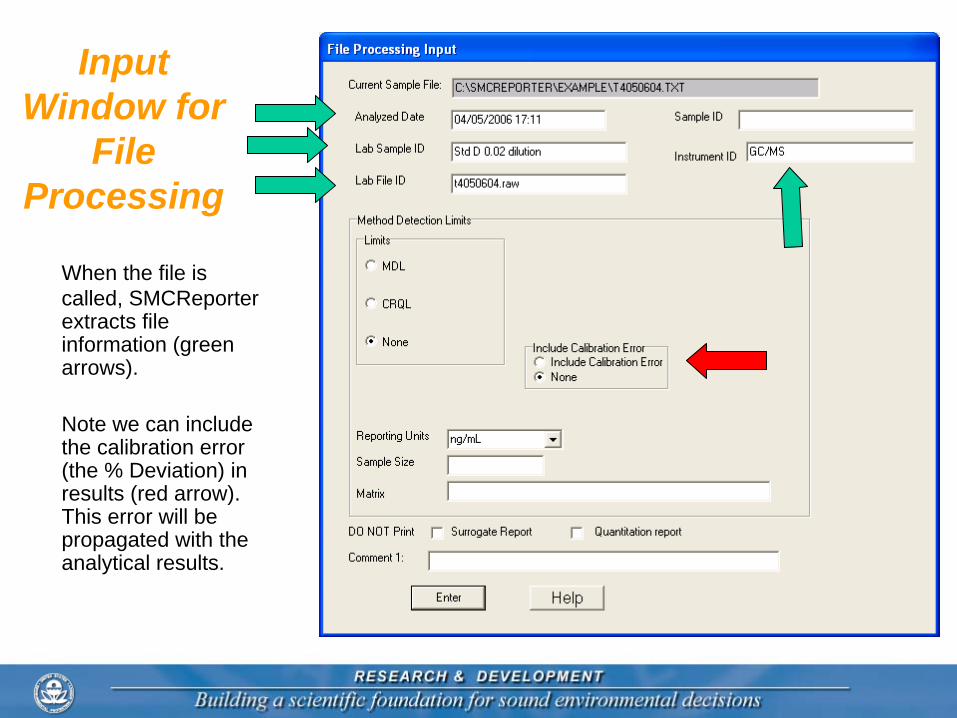
Input Window for

File Processing

When the file is called, SMCReporter extracts file information (green arrows).

Note we can include the calibration error (the % Deviation) in results (red arrow). This error will be propagated with the analytical results.

Sample Information• Leave the “List MDL” “no” checked.• Leave the reporting units as ng/mL.• Enter 5 for the sample size (5 mL).• Enter “Water” for matrix.• The fields Sample ID and comment 1 are for

entering sample specific information at this time.

• Check the “DO NOT print surrogate report” box. We will address that report later.

• Click “Enter”. The next window should look like the following slide.

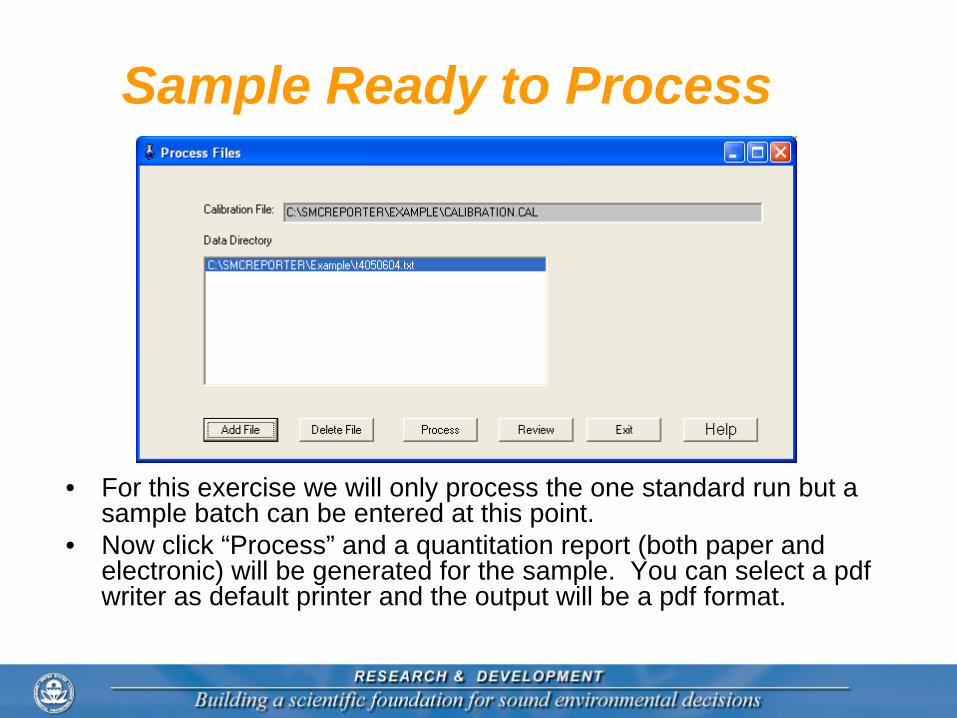
Sample Ready to Process

• For this exercise we will only process the one standard run but a sample batch can be entered at this point.

• Now click “Process” and a quantitation report (both paper and electronic) will be generated for the sample. You can select a pdf writer as default printer and the output will be a pdf format.

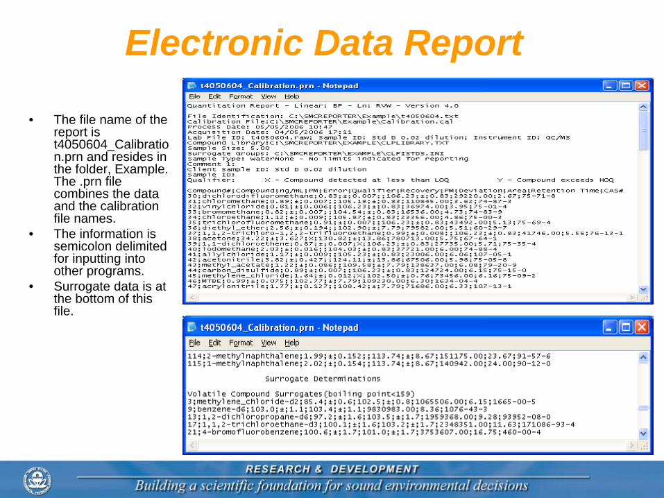
Electronic Data Report

• The file name of the report is t4050604_Calibratio n.prn and resides in the folder, Example. The .prn file combines the data and the calibration file names.

• The information is semicolon delimited for inputting into other programs.

• Surrogate data is at the bottom of this file.

Quantitation Report

Printout

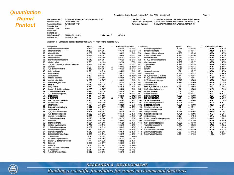
Quantitation Report• Note the header contains a description of all

components that were used to generate the report and the file path.

• Each compound is listed with its calculated concentration, method error, predicted recovery and deviation.

• The paper copy of the report contains the same information as the electronic version but in different formats.

• Note the compounds that are marked with an ‘X’ qualifier. These compounds we remember from reviewing the curve were below the calibration LOQ.

Reporting Limits• File Processing Input window is the means to limit results to only those

above a threshold. The MDL selection allows using this threshold on a compound by compound basis.

• Similar to the MDL option is the CRQL selection. This selection provides both a limit and use of qualifiers consistent with the Superfund CLP contract SOM1.01. With this option values can be reported below the limit (as a percentage) with another qualifier indicating it below the limit.

• A limit file was created for this presentation as the the concentration of the lower calibration point in 5 mL water (5ml_low.mdl).

• The adventurous can create their own limit file. This requires reloading the library, CLPlibrary.txt, and the internal standard file, CLPistds.ini. Then Menu->File->Create/Edit MDL File. Type of limit file (matrix and sample size) are entered and compound limits be entered individually or modify an existing MDL file. See the SMCReporter operating manual for greater detail.

• The next slide presents the format of the file (5ml_low.mdl).

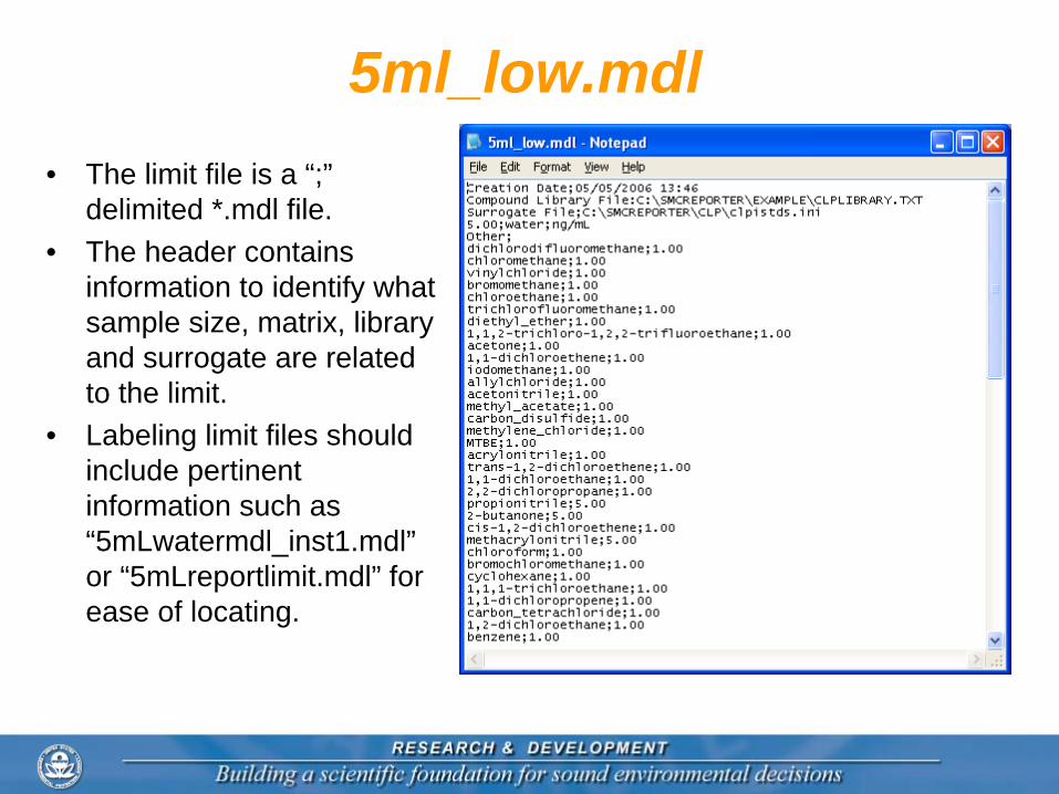
5ml_low.mdl• The limit file is a “;”

delimited *.mdl file.• The header contains

information to identify what sample size, matrix, library and surrogate are related to the limit.

• Labeling limit files should include pertinent information such as “5mLwatermdl_inst1.mdl” or “5mLreportlimit.mdl” for ease of locating.

Process Files with a Reporting Limit

• To observe the use of limits return Quantitation->Process Files and enter the blank file t4050601.txt.

• When the “File Processing Input” window is displayed check the “MDL” option.

• Note that the window retains the previous inputs as new defaults.

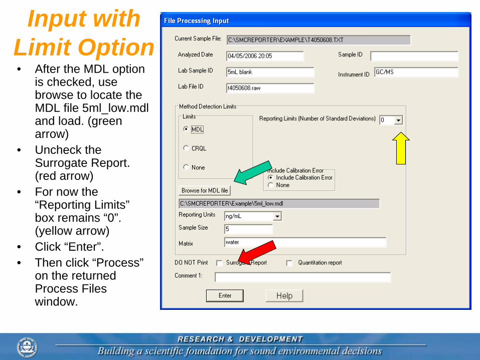
Input with Limit Option• After the MDL option

is checked, use browse to locate the MDL file 5ml_low.mdl and load. (green arrow)

• Uncheck the Surrogate Report. (red arrow)

• For now the “Reporting Limits” box remains “0”. (yellow arrow)

• Click “Enter”.• Then click “Process”

on the returned Process Files window.

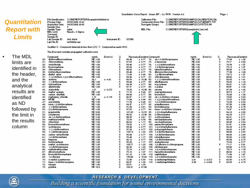
Quantitation Report with

Limits

• The MDL limits are identified in the header, and the analytical results are identified as ND followed by the limit in the results column

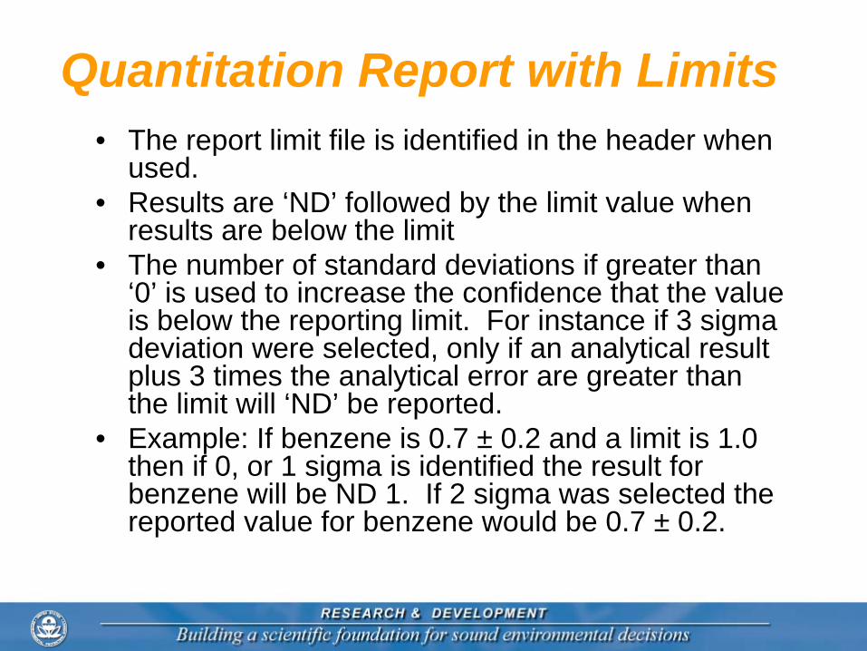
Quantitation Report with Limits• The report limit file is identified in the header when

used.• Results are ‘ND’ followed by the limit value when

results are below the limit• The number of standard deviations if greater than

‘0’ is used to increase the confidence that the value is below the reporting limit. For instance if 3 sigma deviation were selected, only if an analytical result plus 3 times the analytical error are greater than the limit will ‘ND’ be reported.

• Example: If benzene is 0.7 ± 0.2 and a limit is 1.0 then if 0, or 1 sigma is identified the result for benzene will be ND 1. If 2 sigma was selected the reported value for benzene would be 0.7 ± 0.2.

QC report• The QC report contains the equations used to

generate the results (paper copy presents a graphic presentation of effects observed).

• The QC report contains the method 8261 calculations on the monitoring surrogates as individual compounds and as volatile, non-purgeable volatile, and semivolatile groupings.

• With the exception of graphics the electronic version of the QC report contains the same data as the printed report.

QC Report• The QC Report is 2 pages when

printed. An electronic version is also created.

• An Internal standard report presenting the relationships of recovery to boiling point and relative volatility are presented as a single page.

• The surrogates data are presented on the second page.

• The electronic QC report is included in a *.SQL file. To read the file use notepad and open t4050608.SQC.

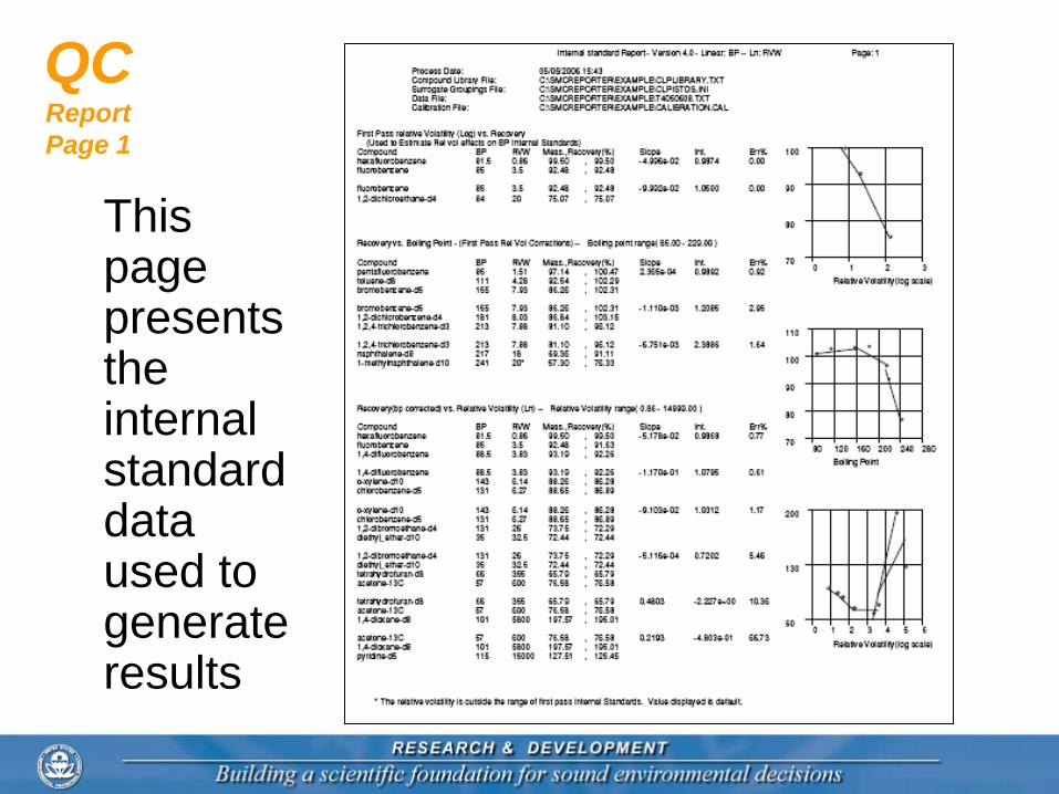
QC Report Page 1

This page presents the internal standard data used to generate results

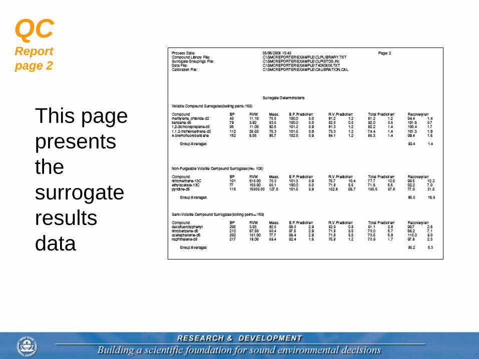
QC Report page 2

This page presents the surrogate results data

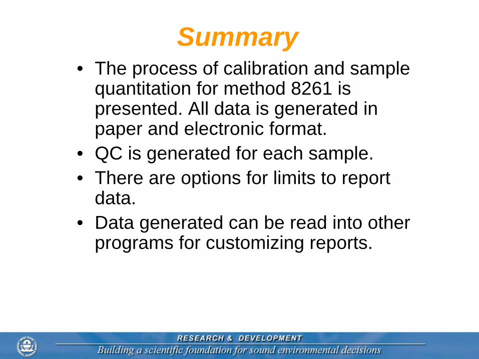
Summary• The process of calibration and sample

quantitation for method 8261 is presented. All data is generated in paper and electronic format.

• QC is generated for each sample.• There are options for limits to report

data.• Data generated can be read into other

programs for customizing reports.