Embed Size (px)
Citation preview
Probability-of-default curve calibration and validation of the internal rating systems 1
Probability-of-default curve calibration and the validation of internal rating systems
Natalia Nehrebecka Narodowy Bank Polski, Department of Econometrics and Statistics, University of Warsaw
Abstract
The purpose of this article is to present calibration methods which give accurate estimations of default probabilities and validation techniques for evaluating calibration power. Applying both these aspects to real data produces accurate verification and conclusions. The empirical analysis was based on individual data from different sources (from the years 2007 to 2012), i.e. from Prudential Reporting, The National Court Register, AMADEUS, and Notoria OnLine.
This article deals with the issue of rating system calibration, i.e. allocation of rating classes to entities in order to ensure that the calibration power of the division created is as high as possible. The methods presented can be divided into two groups. The first contains methods for approximating conditional score distributions for defaults and entities with a good financial standing to a parametric distribution which can be expressed with the use of a density function and distribution functions. The second group covers a number of variants of regression on binary variables denoting the default status of a given company. The use of k-fold cross-validation and repetition of calculations for different master scales and differing data sets means that the results should be highly robust against distribution of the variable in the training set.
Keywords: probability of default, calibration, rating
JEL classification: C13, G24
2 Probability-of-default curve calibration and validation of the internal rating systems
Contents Probability-of-default curve calibration and the validation of internal rating
systems ................................................................................................................................................ 1
Introduction ............................................................................................................................................... 2
Data description ....................................................................................................................................... 5
Calibration and verification using a test for the whole rating system ............................... 7
1. The quasi-moment-matching method [Tasche, 2009] .......................................... 7
2. Methods of approximating parametric distribution ............................................... 7
2.1. Skew normal distribution .......................................................................................... 7
2.2. Scaled beta distribution ............................................................................................ 9
2.3. Asymmetric Laplace distribution .......................................................................... 10
2.4. Asymmetric Gauss distribution ............................................................................. 12
3. Regression analysis and other methods .................................................................... 13
3.1. An approach based on ROC and CAP curves .................................................. 13
3.2 Logit and probit model, complementary log-log (CLL) function, cauchit function .......................................................................................................................... 15
3.3 Platt scaling .................................................................................................................... 16
3.4 Transformation function ........................................................................................... 16
3.5 Broken curve model .................................................................................................... 17
3.6 Isotonic regression ...................................................................................................... 18
4. Verification using a test for the whole rating system ............................................... 19
Conclusion ................................................................................................................................................ 21
Bibliography ............................................................................................................................................ 22
Introduction
Appropriate risk assessment is one of the most important aspects of the activities of financial institutions. In 1999, the Basel Committee on Banking Supervision published several proposal for changes to the current regulations in terms of the capital adequacy structure of financial institutions, which contributed to the preparation of the New Capital Agreement, known as Basel II. The main modification proposed was the reinforcement of the risk management process in the banking sector. One of the key changes in this area was the introduction of the possibility of internal risk management, and therefore the determination of minimal capital requirements. In particular, the bank can select among three approaches. The first of them, which is a continuation of the approach contained in the previous regulation, obliges the bank
Probability-of-default curve calibration and validation of the internal rating systems 3
to maintain the ratio between the minimum capital requirements and the sum of risk-weighted assets at the level of 8%, where the weights are determined by the national regulatory body. As part of the second approach, called IRB (Internal Rating Based), the bank is obliged to prepare an internal estimation of the likelihood of the obligation not being fulfilled (probability of default). The other risk parameters, such as the loss coefficient arising from the failure to fulfil the commitment (loss given default) and the exposure at the time of insolvency (exposure at default) are provided by the regulatory body. The third and at the same time the broadest approach, known as Advanced IRB, enables banks to estimate all risk parameters.
Each bank is obliged, using one of the IRB approaches, to estimate the likelihood of insolvency for each loan granted. A popular method of achieving this is credit scoring. Financial institutions can use external scoring or rating assessments (external rating approach); however, they are applicable to only a small number of the largest business entities. In the vast majority of cases an internally developed risk assessment method (internal rating approach) is used. The use of the bank's own rating boards, called master scales, is a common practice. Entities with low risk levels are grouped together and assigned to one rating class. Each rating class has a top and bottom threshold expressed by the default probability, as well as an average value. The allocation of a given entity to one of the rating classes automatically determines its default probability, which is equal to the average value for the given class. The number of classes depends on the bank's individual approach; however, at least seven classes are required for solvent entities. Usually, lower probability values are assigned to the "upper" classes, which are denoted by digits or appropriate abbreviations, such as "AAA". This is, therefore, a process of discretization of the default probability estimations. On the one hand this approach causes a certain loss of accuracy; on the other it has several important benefits. Firstly, it facilitates further aggregate analysis, simplifies the reporting and model monitoring process. Secondly, it allows for expert knowledge to be used by way of relocation of entities to higher or lower rating classes.
The default probability determination model and the master scale are known as the rating system. This is used to forecast the default probability of each entity, expressed by a rating class. There are two approaches used to establish a rating system. The first, called PIT (point in time), assumes maximum adjustment to changes resulting from the business cycle. The default probability estimation includes individual and macroeconomic components. A high level of migration of units to lower classes is expected in a period of economic growth, and to higher classes at a time of crisis. The second approach, known as TTC (trough the cycle), maximally reduces the influence of the macroeconomic component. All changes are only determined by changes in the individual estimation component, while the percentage share of entities should remain relatively unchanged (Heitfeld, 2005). There is also a broad range of intermediate hybrid approaches, which include individual elements of both the above methods.
This article deals with the issue of rating system calibration, i.e. the allocation of rating classes to entities in order to ensure that the calibration power of the division created is as high as possible. At first, the shape of the function depicting the transition of score into default probability is estimated. The methods presented can be divided into two groups. The first contains the methods for approximating the conditional score distributions of defaults and entities with a good financial standing to their parametric distribution, which can be expressed with the use of a density function and distribution functions. Taking into consideration that these distributions
4 Probability-of-default curve calibration and validation of the internal rating systems
are usually skewed either rightward or leftward of the median, only those types of distribution that allow for a description of both density function asymmetry variants with the use of the appropriate parameters (e.g. asymmetric Gauss distribution, asymmetric Laplace distribution, skew normal distribution and scaled beta distribution) are described. On this basis, and with the use of Bayes’ formula, it is possible to define PD values. These methods are recommended for the purpose of calibrating a score which is not interpreted as a probability (e.g. the score as a result of discriminant analysis).
The second group covers a number of variants of regression on binary variables denoting the default status of a given company. These are universal methods which facilitate the calibration of a score which can be interpreted as a probability (e.g. the score as a result of logistic regression). Firstly, apart from the most popular transition functions (probit and logit), others have also been suggested: cauchit and the complementary log-log function. Another alternative is the application of Platt scaling and Box-Cox transformations to the explanatory variable. The polygonal curve model can also be used for each regression, and a further option is the quasi-moment-matching method and isotonic regression. Based on the probability values found, the rating is allocated with the use of a master scale with set threshold values for individual classes.
Regarding the fact that the main purpose of using the rating system is risk assessment determined in terms of probability, the verification of calibration power is the main part of validation. As noted by Blöchlinger and Leippold (2006), inappropriately calibrated probabilities result in significant losses, even if differences seem to be small. This is a difficult task, because it is impossible to assess the real probability for every assessed unit; in statistical terms it is a latent variable. To solve this problem, it is necessary to use rating classes that are intended to include units of similar risk. Therefore, calibration validation is a comparison of valued ex-ante probabilities and the observed ex-post indicators of insolvency for particular classes, as well as the verification of the significance of statistical differences between those indicators.
While validating model calibration, it is worth testing the calibration power of individual classes, as well as the entire rating system. Testing individual classes mainly involves the binomial test, with all its modifications. A crucial aspect here is to take into consideration the default correlation between entities. Therefore three additional tests will be carried out: the one-factor-model, the moment matching approach and granularity adjustment. While assessing the calibration power of the rating system on the basis of multiple tests carried out on individual classes, the error of decreasing the value of the established p-value level is made. One solution to this problem is to use the Bonferroni or Sidak correction. Another method is to follow the Holm, Hochberg or Hommel procedures. The most popular test of the entire rating system is the Hosmer-Lemeshow test, which involves examination of the differences between observed and the estimated default probability. For the purpose of this research, the Spiegelhalter and Blöchlinger tests were also used; these facilitate verification of the calibration power achieved in a different manner to the Hosmer-Lemeshow test.
The basic purpose of this article is to present calibration methods which provide accurate estimations of default probabilities and validation techniques of calibration power. Using those both aspects on real data provides accurate verification and appropriate conclusions. The subject matter of this article is important and actual, as there is no consensus among practitioners regarding the selection of calibration
Probability-of-default curve calibration and validation of the internal rating systems 5
methods and ways of testing them, so the comparison of methods constitutes a significant added value. According to the author’s best knowledge, some methods will be used for the first time with regard to rating systems calibration. This also confirms the significant value of this work.
Two main research questions will be addressed. The first seeks to verify whether there is a calibration method that gives estimations of probabilities of significantly better quality in logistic regression than others. One of the main assumptions of the new regulation was that banks should be free to select a method for insolvency probability estimation. Logistic regression is the method usually used by banks. This method is also recommended by some Analytics1. Comparing the precision of estimates obtained by means of different approaches will provide an unambiguous evaluation of the quality of the models used.
The second question concerns rating system structure: does the number of rating classes really impact calibration quality? Breinlinger et al. (2003) proved that by increasing the number of classes, at other fixed parameters, the amount of minimum capital requirements decreases. They also found that with a large number of classes it is impossible to meet assumptions concerning the monotonicity of insolvency probability. This might be caused by a significant worsening of estimation calibration. A detailed determination regarding the number of rating classes used is a rarely mentioned but crucial problem, especially for the rating system structure process.
The conclusions presented in this article are mainly directed to banking sector employees concerned with identifying the best way to calibrate internal credit risk systems. A detailed presentation and comparison of different methods allows for a comparison of particular approaches and the selection of the best one. The part of this work that concerns the testing process may be a valuable source of information for validators of risk models.
Data description
The empirical analysis was based on the individual data from different sources (from the years 2007 to 2012):
− Data on banking defaults are drawn from Prudential Reporting (NB300) managed by Narodowy Bank Polski. The Act of the Board of the Narodowy Bank Polski no. 53/2011, dated 22 September 2011 concerning the procedure for and detailed principles of the handing over by banks to the Narodowy Bank Polski data, indispensable for monetary policy, for the periodical evaluation of monetary policy, evaluation of the financial situation of banks and banking sector risks.
− Data on insolvencies/bankruptcies come from a database managed by The National Court Register (KRS), which is the national network of official business register.
− Financial statement data (AMADEUS (Bureau van Dijk); Notoria OnLine). Amadeus (Bureau van Dijk) is a database of comparable financial and business information on Europe's biggest 510,000 public and private companies by assets.
1 CRISIL Global Research & Analytics, Credit Risk Estimation Techniques.
6 Probability-of-default curve calibration and validation of the internal rating systems
Amadeus includes standardized annual accounts (consolidated and unconsolidated), financial ratios, sectoral activities and ownership data. A standard Amadeus company report includes 25 balance sheet items; 26 profit-and-loss account items; and 26 ratios. Notoria OnLine is the standardized format of financial statements for all companies listed on the Stock Exchange in Warsaw.
The following sectors were taken from the Polish Classification of Activities 2007 sample: section A (Agriculture, forestry and fishing), K (Financial and insurance activities). The following legal forms were analyzed: partnerships (unlimited partnerships, professional partnerships, limited partnerships, joint stock-limited partnerships); capital companies (limited liability companies, joint stock companies); and civil law partnerships, state owned enterprises, foreign enterprises.
For the definition of the total number of obligors the following selection criteria were used:
− the company is existent (operating and not liquidated/in liquidation) throughout the entire respective year;
− the company is not in default at the beginning of the year;
− the total exposure reported to be at least 1.5 Mio EUR for each reporting date.
The dataset, after its initial preparation and while keeping only those observations upon which the model can be based, contained 5091 records. However, the number of observations marked as “bad” was 298 (Table 1).
General statistics for 2012
Source: author’s own calculation
Table 1
Number of Obligors
Thereof Insolvent
Thereof defaulted
Insolvency Rate
Default rate
5091 28 298 0,55% 5,85%
The preliminary stage was the implementation of the scoring model with the use
of the Nehrebecka approach (2015). On the basis of this model, point scores were achieved for each enterprise. The value of the score was interpreted by an undefined scoring model. This approach is based on the assumption that this dependence (which is not necessarily linear) is monotonic; that is, that a lesser value correlates to a higher probability of the default state.
The score distribution was rescaled so that the values fell between 0 and 1. This is caused mainly by the application of the root in certain calibration methods. With this modified variable score and a variable binary defining the default state, a validation of the discriminatory power of the model was carried out. AUC, AR, the Pietra index, the Information Value index, and the Kolmogorov-Smirnov test were used. A master scale employed by KBC bank (9 classes) in 2011, for corporate clients in Pekao bank (9 classes) in 2013, in Millenium bank (14 classes) in 2011, and in ING bank (19 classes) in 2012 was used. From the research point of view, it is extremely interesting to ascertain whether the quality of the calibration depends on the master scale.
Probability-of-default curve calibration and validation of the internal rating systems 7
Calibration and verification using a test for the whole rating system
The results presented present the assessment of the function of the transformation of the score into a default probability, which was used to create a rating for the units. Special attention should be paid to the shape of the function for low probability values, as typically the majority of classes used in master scales cover the first 20% of the probability of the default state. The relatively small differences in models for low probabilities will result in relatively large changes in the rating structure. The tests which were carried out allow us to assess the various calibration methods.
1. The quasi-moment-matching method [Tasche, 2009]
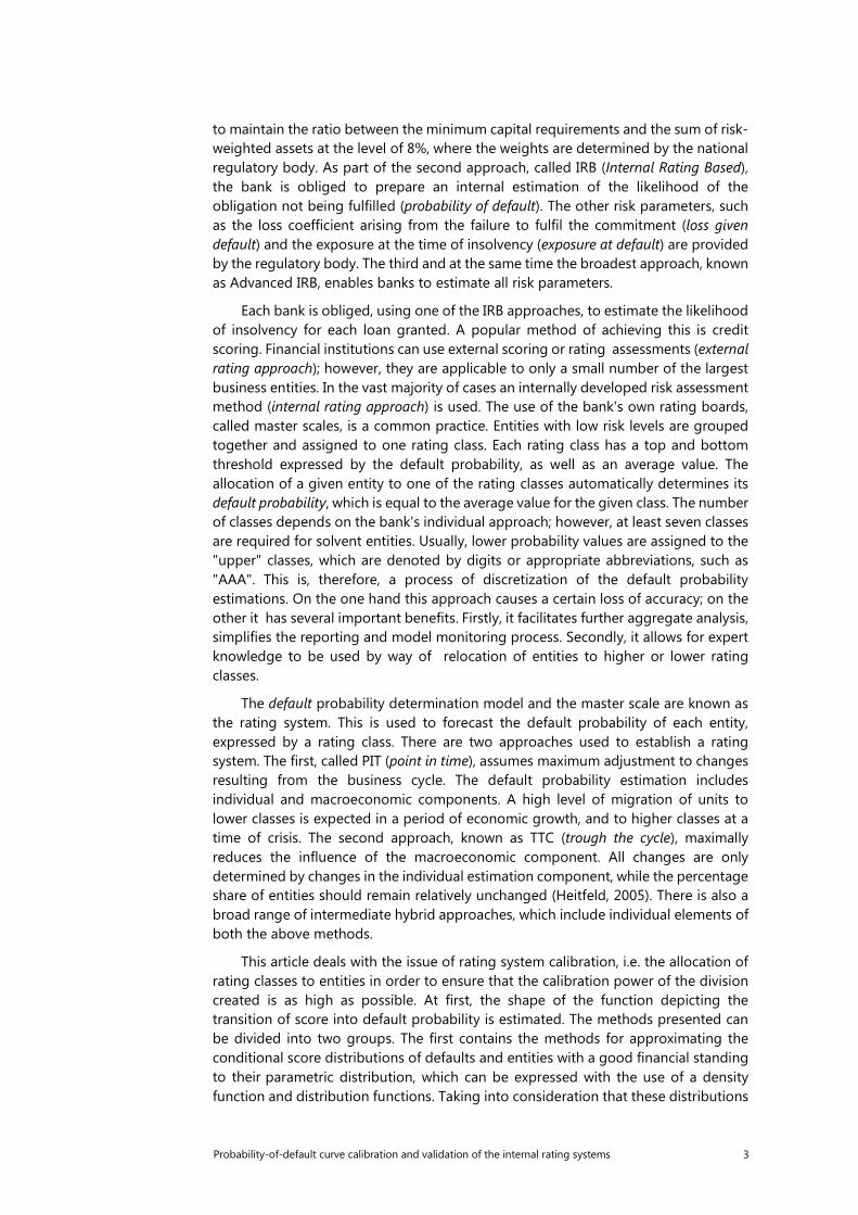
In order to use the quasi-moment-matching method, the target PD value must be established, assumed as the participation of the units in the default state of the total units, and the target value of the AUC (Cumulative Accuracy Profile), which has been determined according to the following formula:
𝐴𝐴𝐴𝐴𝐴𝐴 = (𝑛𝑛𝐷𝐷𝑛𝑛𝑁𝑁𝐷𝐷)−1��𝛿𝛿𝑦𝑦𝑗𝑗(𝑥𝑥𝑖𝑖)𝑛𝑛𝑁𝑁𝑁𝑁
𝑗𝑗=1
𝑛𝑛𝑁𝑁
𝑖𝑖=1
[1]
where: 𝑛𝑛𝐷𝐷 - the number of defaulted borrowers, 𝑛𝑛𝑁𝑁𝐷𝐷 - number of surviving (non-
defaulted) borrowers, 𝛿𝛿𝑤𝑤(𝑧𝑧) = �10 𝑤𝑤ℎ𝑒𝑒𝑒𝑒𝑒𝑒
where 𝑧𝑧 ≤ 𝑤𝑤𝑧𝑧 > 𝑤𝑤.
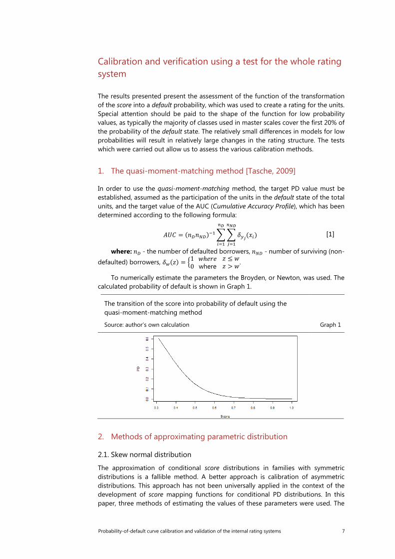
To numerically estimate the parameters the Broyden, or Newton, was used. The calculated probability of default is shown in Graph 1.
The transition of the score into probability of default using the quasi-moment-matching method
Source: author’s own calculation Graph 1
2. Methods of approximating parametric distribution
2.1. Skew normal distribution
The approximation of conditional score distributions in families with symmetric distributions is a fallible method. A better approach is calibration of asymmetric distributions. This approach has not been universally applied in the context of the development of score mapping functions for conditional PD distributions. In this paper, three methods of estimating the values of these parameters were used. The
8 Probability-of-default curve calibration and validation of the internal rating systems
first of them (MLM1) used the approach described by Dey (2010), involving the numeric estimation of the parameters 𝜇𝜇, 𝜎𝜎 and 𝜆𝜆 of the skew normal distribution:
𝑓𝑓(𝑥𝑥) =2𝜎𝜎∗ 𝜙𝜙 �
𝑥𝑥 − 𝜇𝜇𝜎𝜎
� ∗ Φ�𝜆𝜆 ∗𝑥𝑥 − 𝜇𝜇𝜎𝜎
� [2]
where: 𝜇𝜇 − mean, 𝜎𝜎 – variance, 𝜆𝜆 – skew, 𝜙𝜙() – density of standard normal distribution, Φ( ) − distribution.
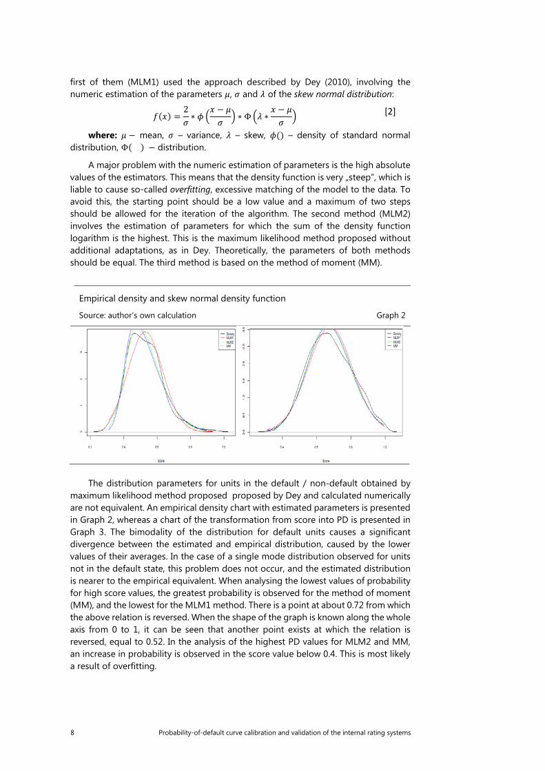
A major problem with the numeric estimation of parameters is the high absolute values of the estimators. This means that the density function is very „steep”, which is liable to cause so-called overfitting, excessive matching of the model to the data. To avoid this, the starting point should be a low value and a maximum of two steps should be allowed for the iteration of the algorithm. The second method (MLM2) involves the estimation of parameters for which the sum of the density function logarithm is the highest. This is the maximum likelihood method proposed without additional adaptations, as in Dey. Theoretically, the parameters of both methods should be equal. The third method is based on the method of moment (MM).
Empirical density and skew normal density function
Source: author’s own calculation Graph 2
The distribution parameters for units in the default / non-default obtained by
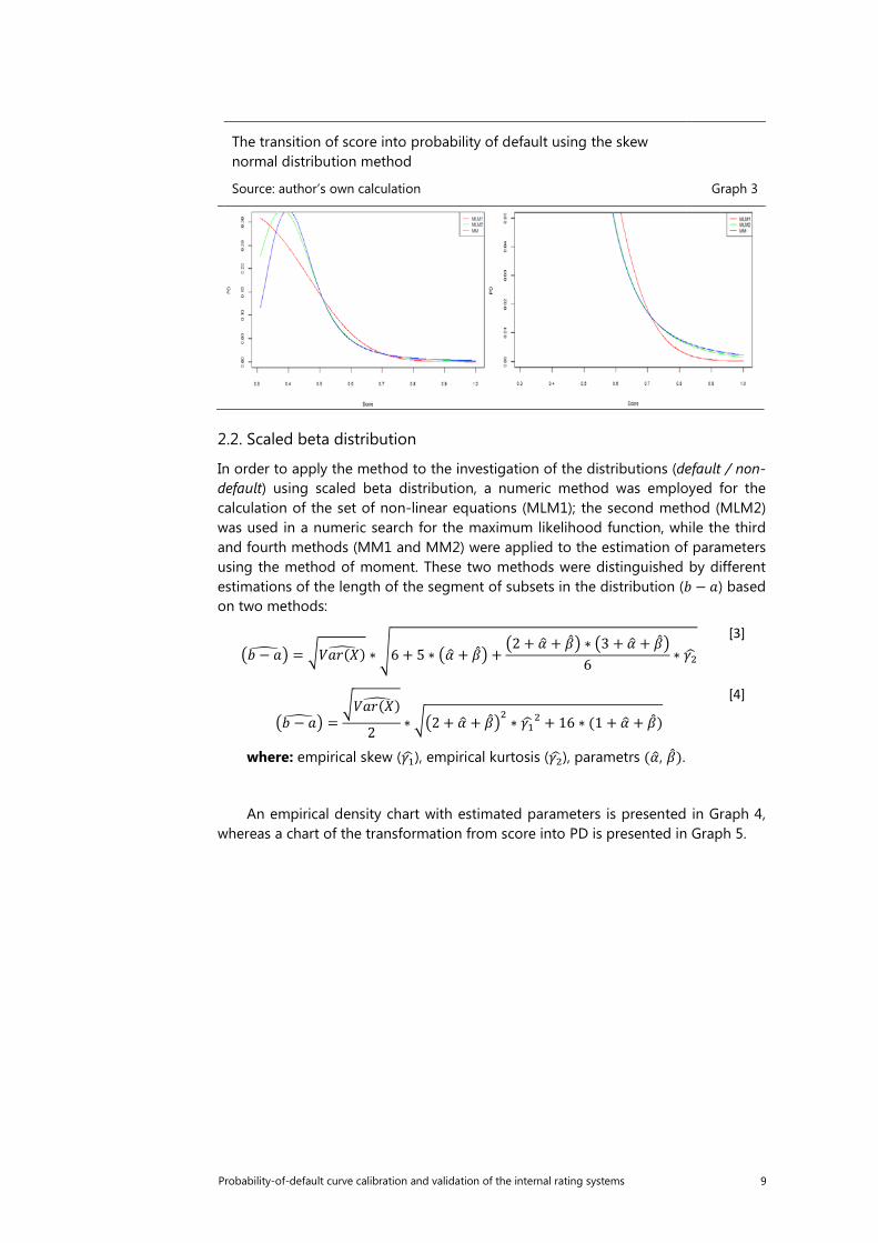
maximum likelihood method proposed proposed by Dey and calculated numerically are not equivalent. An empirical density chart with estimated parameters is presented in Graph 2, whereas a chart of the transformation from score into PD is presented in Graph 3. The bimodality of the distribution for default units causes a significant divergence between the estimated and empirical distribution, caused by the lower values of their averages. In the case of a single mode distribution observed for units not in the default state, this problem does not occur, and the estimated distribution is nearer to the empirical equivalent. When analysing the lowest values of probability for high score values, the greatest probability is observed for the method of moment (MM), and the lowest for the MLM1 method. There is a point at about 0.72 from which the above relation is reversed. When the shape of the graph is known along the whole axis from 0 to 1, it can be seen that another point exists at which the relation is reversed, equal to 0.52. In the analysis of the highest PD values for MLM2 and MM, an increase in probability is observed in the score value below 0.4. This is most likely a result of overfitting.
Probability-of-default curve calibration and validation of the internal rating systems 9
The transition of score into probability of default using the skew normal distribution method
Source: author’s own calculation Graph 3
2.2. Scaled beta distribution
In order to apply the method to the investigation of the distributions (default / non-default) using scaled beta distribution, a numeric method was employed for the calculation of the set of non-linear equations (MLM1); the second method (MLM2) was used in a numeric search for the maximum likelihood function, while the third and fourth methods (MM1 and MM2) were applied to the estimation of parameters using the method of moment. These two methods were distinguished by different estimations of the length of the segment of subsets in the distribution (𝑏𝑏 − 𝑎𝑎) based on two methods:
�𝑏𝑏 − 𝑎𝑎� � = �𝑉𝑉𝑎𝑎𝑒𝑒(𝑋𝑋)� ∗�6 + 5 ∗ �𝛼𝛼� + �̂�𝛽� +�2 + 𝛼𝛼� + �̂�𝛽� ∗ �3 + 𝛼𝛼� + �̂�𝛽�
6∗ 𝛾𝛾2�
[3]
�𝑏𝑏 − 𝑎𝑎� � =�𝑉𝑉𝑎𝑎𝑒𝑒(𝑋𝑋)�
2∗ ��2 + 𝛼𝛼� + �̂�𝛽�2 ∗ 𝛾𝛾1�
2 + 16 ∗ (1 + 𝛼𝛼� + �̂�𝛽)
[4]
where: empirical skew (𝛾𝛾1� ), empirical kurtosis (𝛾𝛾2� ), parametrs (𝛼𝛼�, �̂�𝛽).
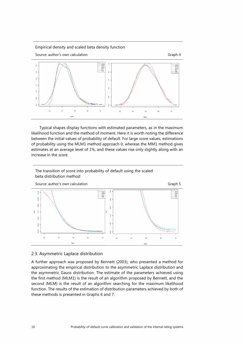
An empirical density chart with estimated parameters is presented in Graph 4, whereas a chart of the transformation from score into PD is presented in Graph 5.
10 Probability-of-default curve calibration and validation of the internal rating systems
Empirical density and scaled beta density function
Source: author’s own calculation Graph 4
Typical shapes display functions with estimated parameters, as in the maximum
likelihood function and the method of moment. Here it is worth noting the difference between the initial values of probability of default. For large score values, estimations of probability using the MLM1 method approach 0, whereas the MM1 method gives estimates at an average level of 1%, and these values rise only slightly along with an increase in the score.
The transition of score into probability of default using the scaled beta distribution method
Source: author’s own calculation Graph 5
2.3. Asymmetric Laplace distribution
A further approach was proposed by Bennett (2003), who presented a method for approximating the empirical distribution to the asymmetric Laplace distribution and the asymmetric Gauss distribution. The estimate of the parameters achieved using the first method (MLM1) is the result of an algorithm proposed by Bennett, and the second (MLM) is the result of an algorithm searching for the maximum likelihood function. The results of the estimation of distribution parameters achieved by both of these methods is presented in Graphs 6 and 7.
Probability-of-default curve calibration and validation of the internal rating systems 11
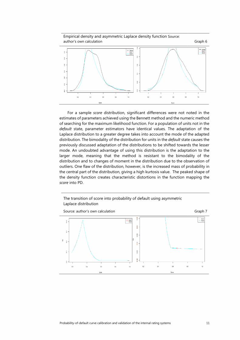
Empirical density and asymmetric Laplace density function Source: author’s own calculation Graph 6
For a sample score distribution, significant differences were not noted in the estimates of parameters achieved using the Bennett method and the numeric method of searching for the maximum likelihood function. For a population of units not in the default state, parameter estimators have identical values. The adaptation of the Laplace distribution to a greater degree takes into account the mode of the adapted distribution. The bimodality of the distribution for units in the default state causes the previously discussed adaptation of the distributions to be shifted towards the lesser mode. An undoubted advantage of using this distribution is the adaptation to the larger mode, meaning that the method is resistant to the bimodality of the distribution and to changes of moment in the distribution due to the observation of outliers. One flaw of the distribution, however, is the increased mass of probability in the central part of the distribution, giving a high kurtosis value. The peaked shape of the density function creates characteristic distortions in the function mapping the score into PD.
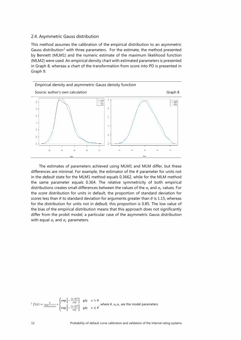
The transition of score into probability of default using asymmetric Laplace distribution
Source: author’s own calculation Graph 7
12 Probability-of-default curve calibration and validation of the internal rating systems
2.4. Asymmetric Gauss distribution
This method assumes the calibration of the empirical distribution to an asymmetric Gauss distribution2 with three parameters. For the estimate, the method presented by Bennett (MLM1) and the numeric estimate of the maximum likelihood function (MLM2) were used. An empirical density chart with estimated parameters is presented in Graph 8, whereas a chart of the transformation from score into PD is presented in Graph 9.
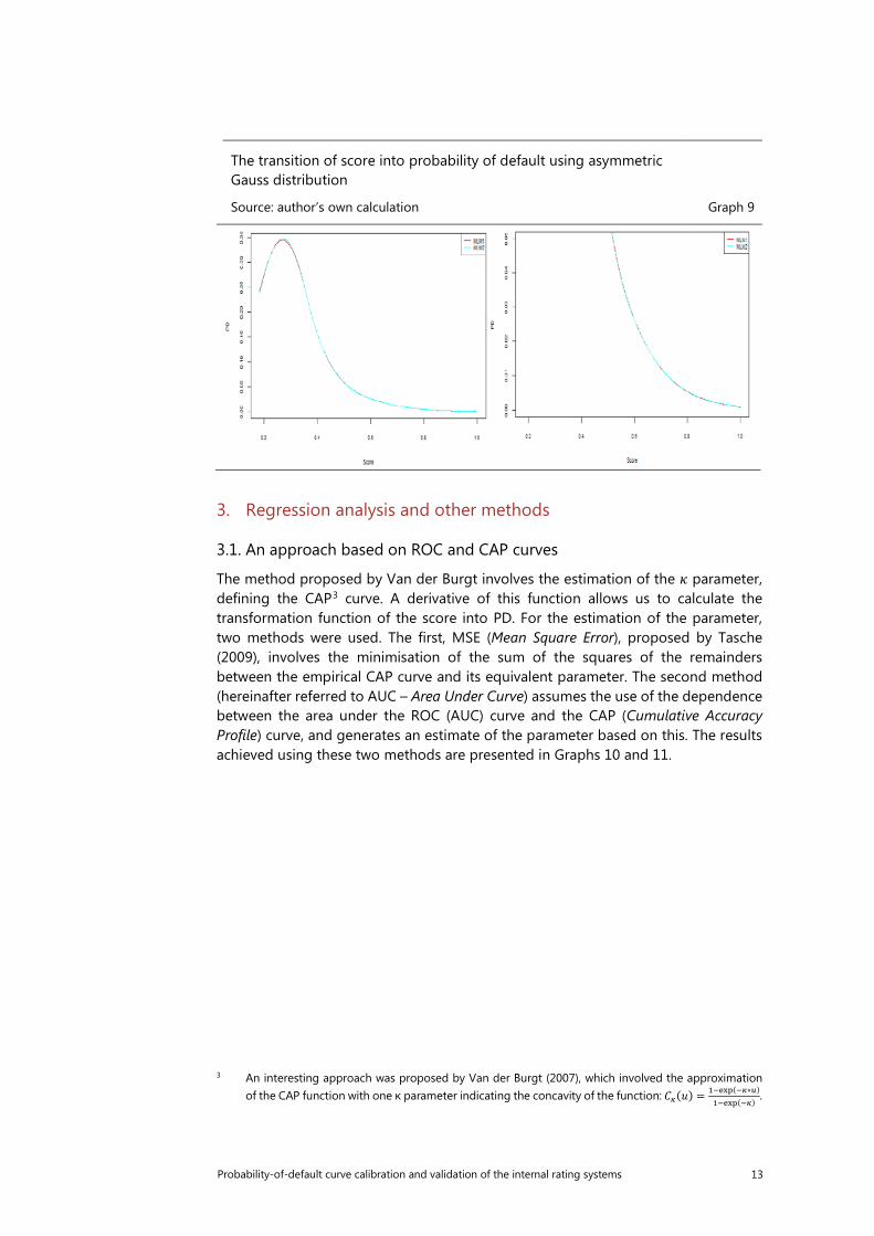
Empirical density and asymmetric Gauss density function
Source: author’s own calculation Graph 8
The estimates of parameters achieved using MLM1 and MLM differ, but these differences are minimal. For example, the estimator of the 𝜃𝜃 parameter for units not in the default state for the MLM1 method equals 0.3662, while for the MLM method the same parameter equals 0.364. The relative symmetricity of both empirical distributions creates small differences between the values of the 𝜎𝜎𝑙𝑙 and 𝜎𝜎𝑟𝑟 values. For the score distribution for units in default, the proportion of standard deviation for scores less than 𝜃𝜃 to standard deviation for arguments greater than 𝜃𝜃 is 1.15, whereas for the distribution for units not in default, this proportion is 0.85. The low value of the bias of the empirical distribution means that this approach does not significantly differ from the probit model, a particular case of the asymmetric Gauss distribution with equal 𝜎𝜎𝑙𝑙 and 𝜎𝜎𝑟𝑟 parameters.
2 𝑓𝑓(𝑥𝑥) = 2√2𝜋𝜋(𝜎𝜎𝑙𝑙+𝜎𝜎𝑟𝑟)
∗ �exp �− (𝑥𝑥−𝜃𝜃)2
2𝜎𝜎𝑟𝑟2� gdy 𝑥𝑥 > 𝜃𝜃
exp �− (𝑥𝑥−𝜃𝜃)2
2𝜎𝜎𝑙𝑙2 � gdy 𝑥𝑥 ≤ 𝜃𝜃
, where 𝜃𝜃, 𝜎𝜎𝑙𝑙 ,𝜎𝜎𝑟𝑟 are the model parameters.
Probability-of-default curve calibration and validation of the internal rating systems 13
The transition of score into probability of default using asymmetric Gauss distribution
Source: author’s own calculation Graph 9
3. Regression analysis and other methods
3.1. An approach based on ROC and CAP curves
The method proposed by Van der Burgt involves the estimation of the 𝜅𝜅 parameter, defining the CAP3 curve. A derivative of this function allows us to calculate the transformation function of the score into PD. For the estimation of the parameter, two methods were used. The first, MSE (Mean Square Error), proposed by Tasche (2009), involves the minimisation of the sum of the squares of the remainders between the empirical CAP curve and its equivalent parameter. The second method (hereinafter referred to AUC – Area Under Curve) assumes the use of the dependence between the area under the ROC (AUC) curve and the CAP (Cumulative Accuracy Profile) curve, and generates an estimate of the parameter based on this. The results achieved using these two methods are presented in Graphs 10 and 11.
3 An interesting approach was proposed by Van der Burgt (2007), which involved the approximation
of the CAP function with one κ parameter indicating the concavity of the function: 𝐴𝐴𝜅𝜅(𝑢𝑢) = 1−exp(−𝜅𝜅∗𝑢𝑢)1−exp(−𝜅𝜅)
.
14 Probability-of-default curve calibration and validation of the internal rating systems
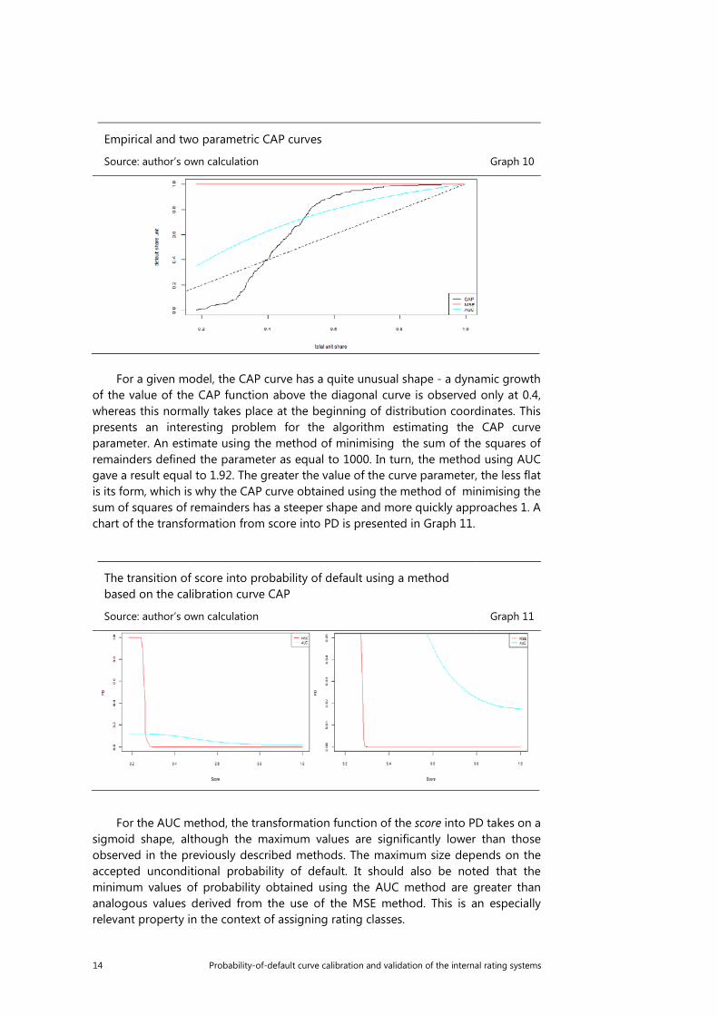
Empirical and two parametric CAP curves
Source: author’s own calculation Graph 10
For a given model, the CAP curve has a quite unusual shape - a dynamic growth of the value of the CAP function above the diagonal curve is observed only at 0.4, whereas this normally takes place at the beginning of distribution coordinates. This presents an interesting problem for the algorithm estimating the CAP curve parameter. An estimate using the method of minimising the sum of the squares of remainders defined the parameter as equal to 1000. In turn, the method using AUC gave a result equal to 1.92. The greater the value of the curve parameter, the less flat is its form, which is why the CAP curve obtained using the method of minimising the sum of squares of remainders has a steeper shape and more quickly approaches 1. A chart of the transformation from score into PD is presented in Graph 11.
The transition of score into probability of default using a method based on the calibration curve CAP
Source: author’s own calculation Graph 11
For the AUC method, the transformation function of the score into PD takes on a sigmoid shape, although the maximum values are significantly lower than those observed in the previously described methods. The maximum size depends on the accepted unconditional probability of default. It should also be noted that the minimum values of probability obtained using the AUC method are greater than analogous values derived from the use of the MSE method. This is an especially relevant property in the context of assigning rating classes.
Probability-of-default curve calibration and validation of the internal rating systems 15
For the MSE method, the shape of the function is most certainly incorrect, as the vast majority of units will be assigned extreme values of probability, nearing either 0 or 1. An effect of this is the assignment of units to extreme classes, either the best or the worst. In spite of this, it was decided not to disqualify this approach. It is not out of the question that the case under consideration is in some way specific, and that for another data set the transformation function may have a gentler shape.
3.2 Logit and probit model, complementary log-log (CLL) function, cauchit function
Another method for the estimation of the function mapping score into PD involves the use of linear regression with a binary explanatory variable. One example of a study which addressed the issue of the construction of a transformation function from a synthetic score indicator into PD is the work done by Neagu et al. (2009). The authors concentrated on finding an alternative to the basic approaches of the logit and probit models, in which PD value is explained by the score constant and variable. As the authors themselves noted with regard to the example analysed, these models overestimate the probability of default for units with a low score, and underestimate for those with a high score. This results mainly from the bias of the score distribution. In order to return the distribution to a normal state, the Box-Cox (B-C) and Box-Tidwell (B-T) transformations were used on a variable score. The use of these transformations is certainly an interesting operation, which allows us to approximate the asymmetrical distribution to a symmetrical one. It is also worth noting that various distributions „react” differently to this transformation. It is harder to obtain a symmetrical shape when transforming a left-bias distribution, as the change in the transformation parameter results in a greater change in bias with regard to the absolute value and also to the diagnostic statistics of the Anderson-Darling test.
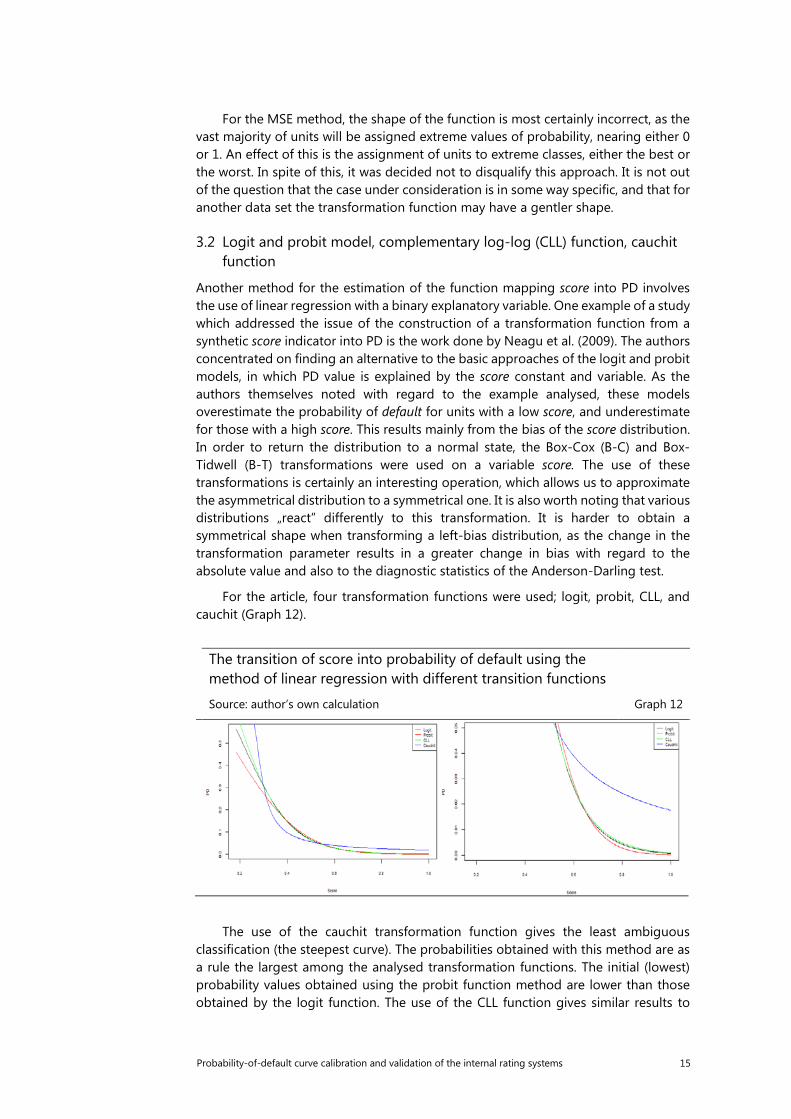
For the article, four transformation functions were used; logit, probit, CLL, and cauchit (Graph 12).
The transition of score into probability of default using the method of linear regression with different transition functions
Source: author’s own calculation Graph 12
The use of the cauchit transformation function gives the least ambiguous classification (the steepest curve). The probabilities obtained with this method are as a rule the largest among the analysed transformation functions. The initial (lowest) probability values obtained using the probit function method are lower than those obtained by the logit function. The use of the CLL function gives similar results to
16 Probability-of-default curve calibration and validation of the internal rating systems
those obtained with the logit function. Concurrent with a decrease in the score, the values of probability rapidly rise, reaching their highest values at a certain moment. It is worth noting the score values, as the probabilities are relatively low. This is crucial in the context of the use of a master scale; a regression using the cauchit function significantly inflates these probabilities. This may cause a significant difference in the classification of units to higher rating classes, which usually require a very low probability.
3.3 Platt scaling
The use of the logit model was also suggested by Platt (1999). Initially, his method was used to transform the results of an SVM (Support Vector Machines) study, belonging to the [-∞, +∞] category, for probabilities within a closed range [0, 1]. The use of the Platt correction for the sample analysed does not significantly influence its results. This is caused mainly by the high number of observations (4112) for which the model was estimated. A significant influence will be observable on the basis of only a few samples.
3.4 Transformation function
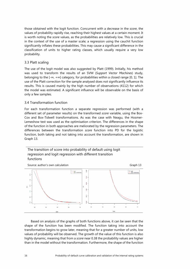
For each transformation function a separate regression was performed (with a different set of parameter results) on the transformed score variable, using the Box-Cox and Box-Tidwell transformations. As was the case with Neagu, the Hosmer-Lemeshow test was used as the optimisation criterion. The differences in the shape of the function in both approaches are meliorated by the regression parameters. The differences between the transformation score function into PD for the logistic function, both taking and not taking into account the transformation, are shown in Graph 13.
The transition of score into probability of default using logit regression and logit regression with different transition functions
Source: author’s own calculation Graph 13
Based on analysis of the graphs of both functions above, it can be seen that the shape of the function has been modified. The function taking into account the transformation begins to grow later, meaning that for a greater number of units, low values of probability will be observed. The growth of the value of this function is also highly dynamic, meaning that from a score near 0.38 the probability values are higher than in the model without the transformation. Furthermore, the shape of the function
Probability-of-default curve calibration and validation of the internal rating systems 17
is gradually flattened out and in the segment from 0 to 0.23 probability values are considerably lower.
3.5 Broken curve model
A further modification of linear regression is the application of a broken curve model. The approach proposed by Neagu assumed a search for a point for which the difference between the results of a „normal” linear regression and the actual percentage of units in default for a given score is the highest. Establishing the method used to calculate the last value was a serious problem, as the authors did not give an unambiguous definition of it. For the purposes of this article it was decided that the value of this function for the score (𝑠𝑠) is equal to the proportion of units in default whose score fell within the range �𝑠𝑠 − 𝑠𝑠𝑠𝑠(𝑠𝑠𝑠𝑠𝑠𝑠𝑟𝑟𝑠𝑠)
10; 𝑠𝑠 + 𝑠𝑠𝑠𝑠(𝑠𝑠𝑠𝑠𝑠𝑠𝑟𝑟𝑠𝑠)
10�. This amount was next
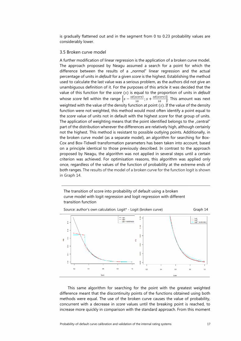
weighted with the value of the density function at point (𝑠𝑠). If the value of the density function were not weighted, this method would most often identify a point equal to the score value of units not in default with the highest score for that group of units. The application of weighting means that the point identified belongs to the „central” part of the distribution wherever the differences are relatively high, although certainly not the highest. This method is resistant to possible outlying points. Additionally, in the broken curve model (as a separate model), an algorithm for searching for Box-Cox and Box-Tidwell transformation parameters has been taken into account, based on a principle identical to those previously described. In contrast to the approach proposed by Neagu, the algorithm was not applied in several steps until a certain criterion was achieved. For optimisation reasons, this algorithm was applied only once, regardless of the values of the function of probability at the extreme ends of both ranges. The results of the model of a broken curve for the function logit is shown in Graph 14.
The transition of score into probability of default using a broken curve model with logit regression and logit regression with different transition function
Source: author’s own calculation. Logit* - Logit (broken curve) Graph 14
This same algorithm for searching for the point with the greatest weighted difference meant that the discontinuity points of the functions obtained using both methods were equal. The use of the broken curve causes the value of probability, concurrent with a decrease in score values until the breaking point is reached, to increase more quickly in comparison with the standard approach. From this moment
18 Probability-of-default curve calibration and validation of the internal rating systems
onwards, as the score values further decreased, the increase in the probability value was significant. The application of the Box-Cox and Box-Tidwell transformations did not cause significant differences other than an increase in the maximum value of probability. When analysing the dependences for low probability values, it can be seen that in comparison to normal linear regression, the application of the broken curve model means that for a greater number of observations, the estimate of the probability of default is obtained at a very low level. In other words, the normal logistic regression overestimates this probability for units with high score values.
3.6 Isotonic regression
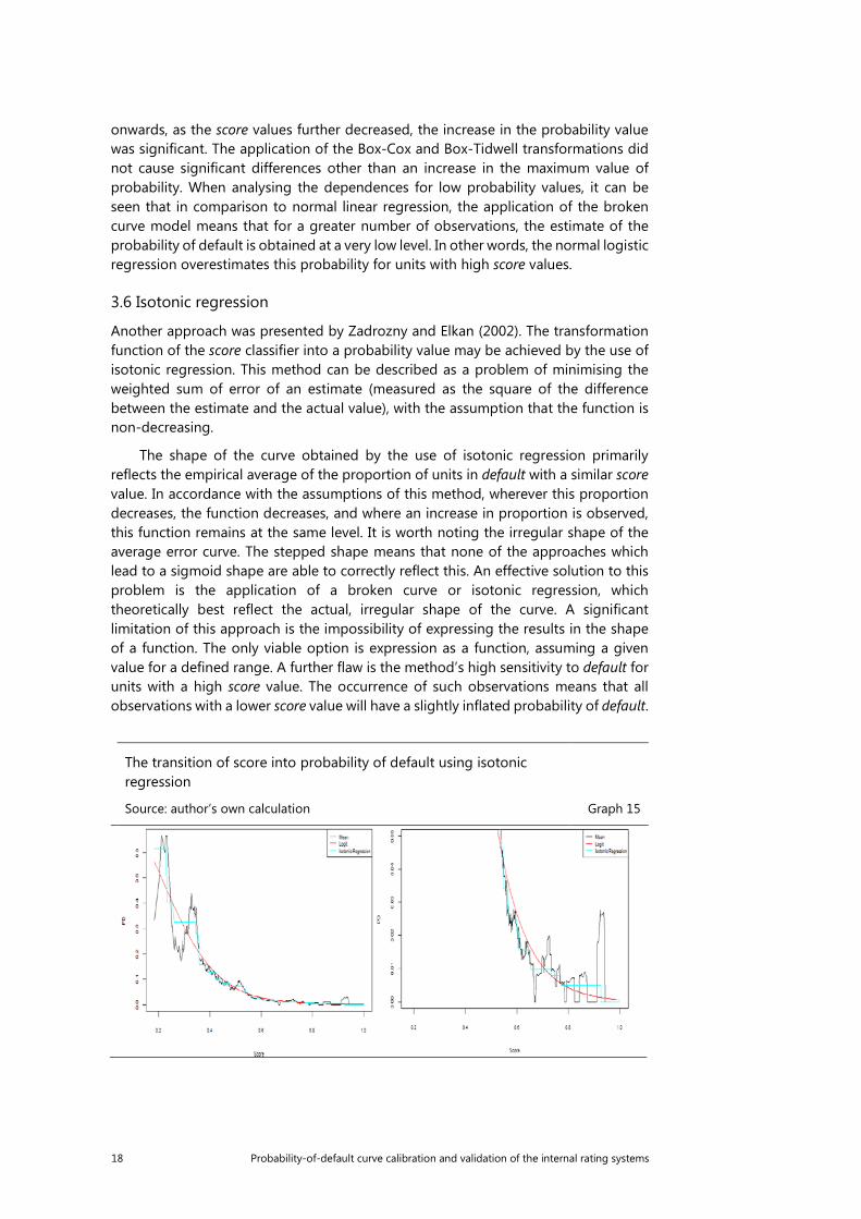
Another approach was presented by Zadrozny and Elkan (2002). The transformation function of the score classifier into a probability value may be achieved by the use of isotonic regression. This method can be described as a problem of minimising the weighted sum of error of an estimate (measured as the square of the difference between the estimate and the actual value), with the assumption that the function is non-decreasing.
The shape of the curve obtained by the use of isotonic regression primarily reflects the empirical average of the proportion of units in default with a similar score value. In accordance with the assumptions of this method, wherever this proportion decreases, the function decreases, and where an increase in proportion is observed, this function remains at the same level. It is worth noting the irregular shape of the average error curve. The stepped shape means that none of the approaches which lead to a sigmoid shape are able to correctly reflect this. An effective solution to this problem is the application of a broken curve or isotonic regression, which theoretically best reflect the actual, irregular shape of the curve. A significant limitation of this approach is the impossibility of expressing the results in the shape of a function. The only viable option is expression as a function, assuming a given value for a defined range. A further flaw is the method’s high sensitivity to default for units with a high score value. The occurrence of such observations means that all observations with a lower score value will have a slightly inflated probability of default.
The transition of score into probability of default using isotonic regression
Source: author’s own calculation Graph 15
Probability-of-default curve calibration and validation of the internal rating systems 19
4. Verification using a test for the whole rating system
After estimating the score transformation function into the probability of default, each unit is assigned a rating, using for this purpose the master scale employed by a given bank. Next, for each rating class an actual default rate is calculated, as the proportion of units in default to units in a given rating class. This data is next used to calculate quality tests for calibration of the rating system. There is a risk that the above analysis may in large part be dependent on the score distribution for the population of bankruptcies and units in good financial condition. It has also been noted that for one subpopulation, this distribution is bimodal, which is not necessarily the rule for other data sets. This feature may have a substantial impact on the results obtained and the conclusions reached on their basis. To avoid this error, a k-fold cross-validation was applied. This involves the division of the original set into k subsets. Next, one subset is chosen as a test case, and the rest are treated as a training cases. The estimates obtained for the training cases were then verified with the test case. This step was repeated k times for another test case. In the validation set, the shape of the transformation function was estimated, and was next applied to the test case. Subsequently, the k obtained for such sets of units, along with the rating assigned to them ,were combined in one set of data based on the average (i.e., the average number of units in a given rating class), on which a calibration test was performed. A value of 4 was assumed for k, which on the one hand allows us to obtain relatively resistant results, and on the other does not significantly extend the process of calculation.
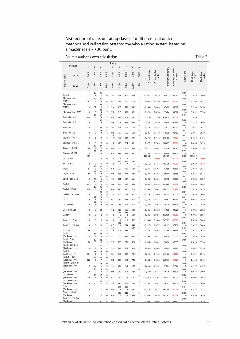
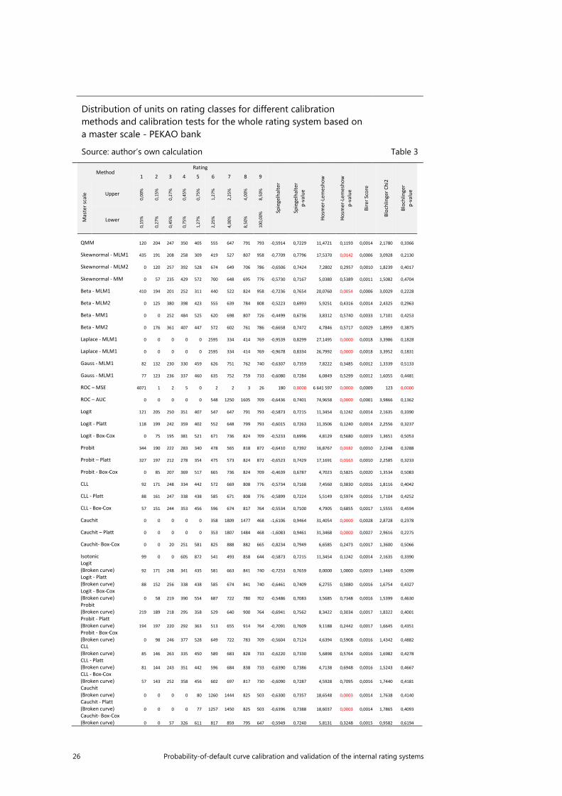
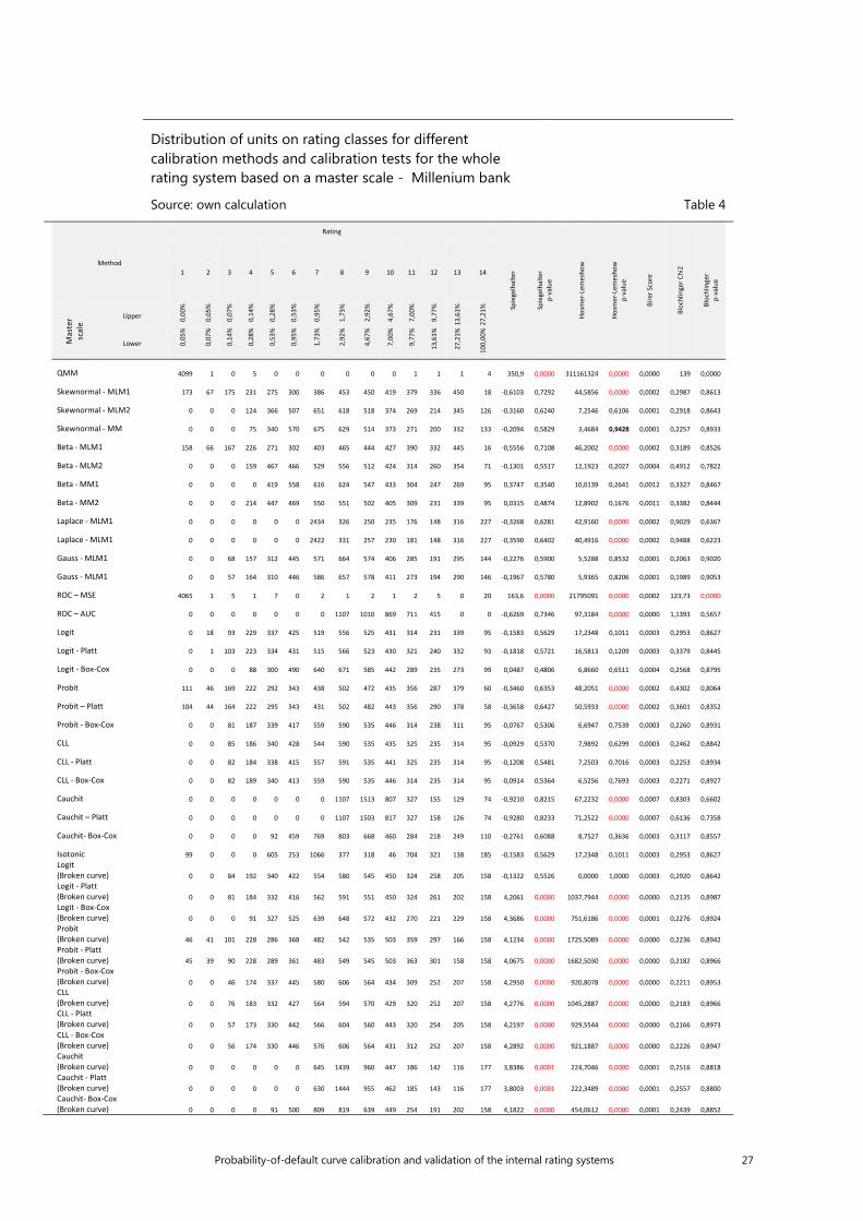
Generally, a higher quality of adaptation is observed for master scales with a smaller number of rating classes (Table 3, Table 4, Table 5, Table 6). For a master scale with 9 classes (KBC and Pekao), lower statistical results are observed in a Spiegelhalter test, higher p-values for the Hosmer-Lemeshow test, lower values for the shape component of the Blöchlinger test, and as a result lower values for the general statistics and higher p-values for this test are observed. This dependence is caused by the fact that with a less granular range, individual rating classes include „wider” ranges of probability of default, leading to an increase in the averages of probability in the initial classes. As has been mentioned previously, the lower the values of probability are, the slower the convergence to an 𝜒𝜒2 distribution is. A further consequence is an increased number of this observances, a fact which is crucial in the context of the asymptomatic properties of calibration tests. The more precise the range, the greater the variance in the ranks of the proportion of defaults, as the measurement becomes more precise and more biased away from the average. With a large number of observations in a given class, the influence of outliers on the actual value of probability for a given class lessens. In other words, the variance of deviation of the actual proportion defaults decreases from the average estimate, meaning that the estimate must be more precise (better calibrated). It must be remembered, however, that the aim of the creation of a rating scale is not to maximise the calibration power of the model it uses. On the assumption that further such dependences can be obtained, and are highly likely to be correct, the most adequate division is one which defines several classes, in extreme cases as few as one. Such an approach is not appropriate. The reason for using master scales is, after all, to maximise business potential, and not to maximise the broadly understood efficiency of the model.
In terms of Spiegelhalter test statistics and their equivalent p-values of ratings ranges using all master scales, on average the highest quality calibration was observed for regression with a cauchit transformation function in the case of master
20 Probability-of-default curve calibration and validation of the internal rating systems
scales comprising 9 classes (KBC, Pekao) for the model approximating the asymmetric Laplace distribution (Laplace-MLM1, Laplace-MLM2), the skew normal approximation method (Skewnormal – MLM1), the scaled beta distribution (Beta – MLM1), and the approximation method using the ROC curved (ROC-AUC). The use of Platt’s correction brings excellent results. A dependence was observed in which the normal method of moment delivers as a result a lower quality of adapted probabilities. The relatively large differences between both methods in the approximation of the ROC curve should also be stressed. Unambiguously for all master scales, a p-value equal to 0.000 is observed for the ROC (ROC-MSE) method of approximating the curve. Additionally, in the case of the Millenium Bank master scale, a p-value equal to 0.000 was also noted for the QMM method, and for regression accounting for a broken curve with transformation functions other than Logit (Broken curve) (logit, probit, cauchit and CLL).
In performing an analysis of the p-value of the Hosmer-Lemeshow test for a range using all master scales, the highest quality is observed for a regression taking into account a broken curve with the logit transformation function. In each case, a value equal to 1 is observed. This is especially important for „large” master scales, in which for the majority of models the p-value was equal to 0.000. It should also be noted that the simple application and interpretation of the results of this test is problematic, as for values of observed probability near 0 or 1 the values of the test statistics approach infinity. For the model of approximation with an asymmetric beta distribution, both of the method of moment deliver an average statistical test value higher by 2*10^12. This is to be expected, as in this method a relatively small number of units is assigned to a relatively high number of classes. If in a particular case this is one unit which is not in default, the probability of default observed for this class with one unit will equal 0, in turn delivering a high statistical test value. Conclusions on the quality of calibration based on the Hosmer-Lemeshow test may thus be made more difficult. For this reason the application of different, alternative approaches such as the Blöchlinger test is exceptionally valuable.
In terms of the general value of the statistics in the Blöchlinger test and their resultant p-values, the worst quality of calibration was obtained when using the two methods of approximating the ROC curve. In turn, the best quality was observed for regression taking into account a broken curve with a logit transformation function, regression with a logit curve, probit, CLL, and cauchit with the Box-Cox transformation. With the exception of regression, for all of these models the quality of calibration rises with the increase in the granularity of the range.
Summing up, the calibration power of the entire rating system was obtained with different calibration methods and different master scales using three tests which took into account k-fold cross-validation. The use of these tests allowed us to study several aspects of high-quality calibration. The Spiegelhalter test verifies the extent to which the estimate of probability for units diverge from the observed proportion of defaults in a given group of units. The shape of the test statistics is regular and is the result of a process of standardisation. A similar zero hypothesis is obtained by the Hosmer-Lemeshow test, though the unit is the rating class, and the statistics have an 𝜒𝜒2 distribution. The Blöchlinger test verifies two basic elements of high-quality calibrations – a size component measured as the average of probability of default with regard to the average proportion of defaults for the entire sample, and a shape component measured as the deviation from the observed ROC curve.
Probability-of-default curve calibration and validation of the internal rating systems 21
In comparing the quality of calibration to normal logistic regression, a set of methods with a significantly better precision of estimates was identified. There are also methods which always give better calibrated estimates of probability when compared to all of the methods applied in the tests. These are regressions that take into account a broken curve with logit transformation, logit regression, probit, CLL, and cauchit with the Box-Cox transformation.
A further conclusion is the considerable improvement in calibration that is achieved when the Box-Cox transformation is taken into account for the regression analysed. A significant increase in the average p-values for the Blöchlinger and Hosmer-Lemeshow tests is observed. The p-values of the Spiegelhalter test remain relatively stable.
In performing an analysis of the calibration with regard to the number of classes in the master scale, a significant decrease in the precision of the estimates of probability can be observed with an increase in the number of classes. This dependence is especially visible for the Blöchlinger test.
Conclusion
The basic aim of this paper was to present methods of calibration that allow us to obtain precise estimates of the probability of default, and techniques of validation based on their calibrating power. The use of k-fold cross-validation and repetition of calculations for different master scales and differing data sets means that the results should be highly resistant for the distribution variable in the training set.
The use of several tests allows us to take into account different definitions of high-quality calibration. The results obtained were not unambiguous, but they do allow us to answer the basic research question. First, we can say that there are methods which deliver considerably better calibrated estimates of probability in comparison with logistic regression estimators. The difference observed is relatively large and also concerns calibration of the system as a whole.
The second research question concerned the quality of calibration for different numbers of classes in the master scales. Using four different approaches (master scales including from 9 to 19 classes), whose sources were bank reports on risk, a decrease in the quality of calibration of the whole rating system was noted, in conjunction with an increase in the number of classes. This dependence is dictated first and foremost by the wider ranges of probability for particular classes, and by the properties of the statistical tests applied.
These conclusions definitely do not fully address the issue of the construction of a model that would give the best calibrated estimates. This issue is highly complex, due mainly to the lack of a single, unambiguous method of calibration and a method of estimating the correlation of default between units. A very interesting development of this study would be the use of simulation techniques and an attempt to take into account the cost (expressed in units of time) for the calculation of samples of various sizes.
22 Probability-of-default curve calibration and validation of the internal rating systems
Bibliography
Agresti A., Coull B. A., Approximate is better than “exact” for interval estimation of binomial proportions, The American Statistician 52.2, 1998, pp. 119-126.
Aickin M., Gensler H., Adjusting for multiple testing when reporting research results: the Bonferroni vs Holm methods, American journal of public health 86.5, 1996, 726-728.
Basel II: International Convergence of Capital Measurement and Capital Standards: A Revised Framework, 2005.
Basel II, International Convergence of Capital Measurement and Capital Standards, 2006.
____ Update on work of the Accord Implementation Group related to validation under the Basel II Framework, Basel Committee Newsletter No. 4, 2005.
Beaver W., Financial ratios as predictors of failure. Journal of Accounting Research 5, 1966, pp. 71-111.
Bennett P. N., Using asymmetric distributions to improve text classifier probability estimates, w: Proceedings of the 26th annual international ACM SIGIR conference on Research and development in information retrieval, ACM, 2003.
Blöchlinger A., Leippold M., Economic benefit of powerful credit scoring, Journal of Banking & Finance, 2006, pp. 851-873.
Blochwitz S., Martin M., When C. S., Statistical approaches to PD validation, The Basel II Risk Parameters. Springer Berlin Heidelberg, 2011, pp. 293-309.
Breinlinger L., Glogova E., Höger A., Calibration of Rating Systems-A First Analysis, Financial Stability Report 5, 2003, pp. 70-81.
Brown L. D., Cai T. T., DasGupta A., Interval estimation for a binomial proportion, Statistical science, 2001, pp. 101-117.
Clopper C. J., Pearson E. S., The use of confidence or fiducially limits illustrated in the case of the binomial, Biometrika, 1934, pp. 404-413.
Dey D., Estimation of the Parameters of Skew Normal Distribution by Approximating the Ratio of the Normal Density and Distribution Functions, 2010.
Edmister R., An empirical test of financial ratio analysis for small business failure prediction, Journal of Financial and Quantitative Analysis 7(2), 1972, pp. 1477-1493.
Engelmann B., Hayden E., Tasche D., Testing rating accuracy, Risk 16 (1), 2003, pp. 82-86.
FritzPatrick P., A Comparison of the Ratios of Successful Industrial Enterprises with Those of Failed Companies, The Accountants Publishing Company, 1932.
Fulmer J. G., A bankruptcy classification model for small firms, Journal of Commercial Bank Lending 66.11, 1984, pp. 25-37.
Güttler A., Liedtke H. G., Calibration of Internal Rating Systems: The Case of Dependent Default Events, Kredit und Kapital 40, 2007, pp. 527-552.
Hamerle A., Liebig T., Rösch D., Benchmarking asset correlations, Risk 16.11, 2003, pp. 77-81.
Probability-of-default curve calibration and validation of the internal rating systems 23
Heitfeld E. A., Dynamics of rating system, in: Basel, Studies on the Validation of Internal Rating Systems, Working Paper No. 14, 2005.
Hochberg Y., A sharper Bonferroni procedure for multiple tests of significance, Biometrika 75.4, 1988, pp. 800-802.
Holm S., A simple sequentially rejective multiple test procedure, Scandinavian journal of statistics, 1979, pp. 65-70.
Mays E, Handbook of credit scoring. Global Professional Publishig, 2001.
____ Credit risk modeling: Design and application. Global Professional Publishing, 1998.
Nagpal K., Bahar R., Measuring default correlation, Risk 14.3, 2001, pp. 129-132.
Neagu R., Keenan S., Chalermkraivuth K., Internal credit rating systems: Methodology and economic value, The Journal of Risk Model Validation 3.2, 2009, pp. 11-34.
Nehrebecka N., Approach to the assessment of credit risk for non-financial corporations. Evidence from Poland, 2015. www.bis.org.
Newcombe R. G., Two-sided confidence intervals for the single proportion: comparison of seven methods, Statistics in medicine 17.8, 1998, pp. 857-872.
Pires A. M., Amado C., Interval estimators for a binomial proportion: Comparison of twenty methods, REVSTAT‒Statistical Journal 6.2, 2008, pp. 165-197.
Platt J., Probabilistic outputs for support vector machines and comparisons to regularized likelihood methods, Advances in large margin classifiers 10.3, 1999, pp. 61-74.
Rauhmeier R., PD-validation: experience from banking practice, The Basel II Risk Parameters. Springer Berlin Heidelberg, 2011, pp. 311-347.
Shaffer J. P., Multiple hypothesis testing, Annual review of psychology 46.1, 1995, 561-584.
Šidák Z., Rectangular confidence regions for the means of multivariate normal distributions, Journal of the American Statistical Association 62.318, 1967, pp. 626-633.
Spiegelhalter D. J., Probabilistic prediction in patient management and clinical trials, Statistics in medicine 5.5, 1986, pp. 421-433.
Tasche D., A traffic lights approach to PD validation, 2003.
____ Estimating discriminatory power and PD curves when the number of defaults is small, 2009.
____ Rating and probability of default validation, w: Bazylejski Komitet Nadzoru Bankowego, Studies on the Validation of Internal Rating Systems. Working Paper No. 14, 2005, pp. 169-196.
____ The art of probability-of-default curve calibration, Journal of Credit Risk 9.4, 2013, pp. 63-103.
____ Validation of internal rating systems and PD estimates, The analytics of risk model validation, 2006, pp. 169-196.
Thomas L. C., Edelman D. B., Crook J. N., Credit scoring and its applications, Siam, 2002.

24 Probability-of-default curve calibration and validation of the internal rating systems
Van der Burgt M. J., Calibrating low-default portfolios, using the cumulative accuracy profile, Journal of Risk Model Validation 1.4, 2008, pp. 17-33.
Wall A., Study of credit barometrics, Federal Reserve Bulletin, 1919, pp. 229–243.
Wallis S., Binomial confidence intervals and contingency tests: mathematical fundamentals and the evaluation of alternative methods, Journal of Quantitative Linguistics 20.3, 2013, pp. 178-208.
Winakor A., Smith R., A Test Analysis of Unsuccessful Industrial Companies, Bulletin no. 31, Bureau of Business research, University of Illinois, 1930.
____ Changes in Financial Structure of Unsuccessful Industrial Corporations, Bulletin no. 51, Bureau of Business Research, University of Illinois, 1935.
Zadrozny B., Elkan Ch., Transforming classifier scores into accurate multiclass probability estimates, Proceedings of the eighth ACM SIGKDD international conference on Knowledge discovery and data mining. ACM, 2002.
Probability-of-default curve calibration and validation of the internal rating systems 25
Distribution of units on rating classes for different calibration methods and calibration tests for the whole rating system based on a master scale - KBC bank.
Source: author’s own calculation Table 2
Method Rating
Spie
gelh
alte
r
Spie
gelh
alte
r p-
valu
e
Hosm
er-L
emes
how
Hosm
er-L
emes
how
p-
valu
e
Bire
r Sco
re
Bloc
hlin
ger
Chi2
Bloc
hlin
ger
p-va
lue
1 2 3 4 5 6 7 8 9 M
aste
r sca
le
Upper 0,00
%
0,10
%
0,20
%
0,40
%
0,80
%
1,60
%
3,20
%
6,40
%
12,8
0%
Lower 0,10
%
0,20
%
0,40
%
0,80
%
1,60
%
3,20
%
6,40
%
12,8
0%
100%
QMM 57 13
7 31
7 46
0 582 727 735 633 46
4 -0,3921 0,6525 9,2857 0,2328 0,000
8 0,9929 0,6087 Skewnormal - MLM1 327
194
253
348 441 584 697 729
539 -0,6614 0,7458 36,4415 0,0000
0,0003 0,7943 0,6722
Skewnormal - MLM2 0 57
249
523 734 799 722 517
511 -0,4636 0,6785 8,7482 0,1882
0,0005 0,7990 0,6706
Skewnormal - MM 0 0 21
4 57
7 778 818 717 502 50
6 -0,3718 0,6450 7,3424 0,1964 0,000
6 0,6332 0,7286
Beta - MLM1 309 18
7 25
3 34
7 440 592 705 757 52
2 -0,6189 0,7320 34,8075 0,0000 0,000
3 0,6180 0,7342
Beta - MLM2 0 0 41
9 53
5 599 713 732 650 46
4 -0,3421 0,6339 4,3948 0,4941 0,000
9 0,7244 0,6961
Beta - MM1 0 0 97 69
8 704 814 791 593 41
5 -0,1602 0,5636 5,3872 0,3705 0,002
6 0,9845 0,6112
Beta - MM2 0 0 45
2 54
2 609 717 725 603 46
4 -0,4065 0,6578 5,6195 0,3450 0,002
2 0,8965 0,6388
Laplace - MLM1 0 0 0 0 238
7 416 394 345 57
0 -0,6560 0,7441 27,3488 0,0000 0,001
0 1,4238 0,4907
Laplace - MLM1 0 0 0 0 237
8 425 384 351 57
4 -0,6773 0,7509 26,6065 0,0000 0,001
0 1,4856 0,4758
Gauss - MLM1 20 10
1 27
0 43
8 648 853 796 518 46
8 -0,4127 0,6601 9,9288 0,1926 0,000
6 0,6840 0,7103
Gauss - MLM1 18 10
0 26
3 44
2 654 861 795 511 46
8 -0,3903 0,6518 9,8438 0,1976 0,000
6 0,6352 0,7279
ROC – MSE 407
1 0 2 6 0 3 3 7 20 163,389
4 0,0000 664179
7 0,0000 0,000
2 123,192
5 0,0000
ROC – AUC 0 0 0 0 0 130
4 148
7 132
1 0 -0,6517 0,7427 60,3700 0,0000 0,000
1 8,0220 0,0181
Logit 57 14
3 31
9 45
8 576 727 750 618 46
4 -0,3861 0,6503 8,1855 0,3165 0,000
9 0,9083 0,6350
Logit - Platt 57 12
7 31
7 45
6 579 730 749 633 46
4 -0,4056 0,6575 8,5176 0,2892 0,000
8 0,8725 0,6464
Logit - Box-Cox 0 20 20
5 49
2 721 861 827 561 42
5 -0,2960 0,6164 3,6196 0,7280 0,001
3 0,9905 0,6094
Probit 231 19
8 26
8 38
4 482 654 712 696 48
7 -0,4829 0,6854 15,1820 0,0337 0,000
6 0,8206 0,6634
Probit – Platt 224 19
3 26
8 37
2 486 646 740 704 47
9 -0,4965 0,6902 15,8352 0,0267 0,000
5 0,8435 0,6559
Probit - Box-Cox 0 0 20
8 48
9 729 873 834 567 41
2 -0,2144 0,5849 3,6169 0,6058 0,001
4 0,8675 0,6481
CLL 20 12
8 29
3 47
1 587 767 784 608 45
4 -0,3632 0,6418 7,5552 0,3734 0,001
0 1,0587 0,5890
CLL - Platt 20 12
3 29
2 45
9 597 763 796 608 45
4 -0,3846 0,6497 7,4704 0,3816 0,001
0 1,1238 0,5701
CLL - Box-Cox 0 0 80 41
4 772 986 906 592 36
2 -0,1353 0,5538 4,4086 0,4922 0,001
5 0,9481 0,6225
Cauchit 0 0 0 0 0 141
2 189
2 587 22
1 -1,3317 0,9085 23,3999 0,0000 0,001
9 4,7105 0,0949
Cauchit – Platt 0 0 0 0 0 140
1 190
3 587 22
1 -1,3336 0,9088 23,3383 0,0000 0,001
9 4,8233 0,0897
Cauchit- Box-Cox 0 0 20 42
1 825 101
4 874 546 41
2 -0,5178 0,6977 3,8313 0,5739 0,001
0 0,8677 0,6480
Isotonic 99 0 0 85
8 106
6 411 284 107
1 32
3 -0,3861 0,6503 8,1855 0,3165 0,000
9 0,9083 0,6350 Logit (Broken curve) 20
131
293
474 592 770 796 621
415 -0,3937 0,6531 0,0000 1,0000
0,0010 0,8410 0,6567
Logit - Platt (Broken curve) 20
123
286
465 597 775 810 624
412 -0,3965 0,6541 7,6606 0,3635
0,0009 1,0528 0,5907
Logit - Box-Cox (Broken curve) 0 0
214
514 759 866 801 524
434 -0,3010 0,6183 3,4684 0,6282
0,0009 0,6681 0,7160
Probit (Broken curve) 124
182
253
405 521 711 814 738
364 -0,4131 0,6602 16,1469 0,0238
0,0009 1,3129 0,5187
Probit - Platt (Broken curve) 120
166
257
401 528 705 833 740
362 -0,4305 0,6666 16,5331 0,0207
0,0009 1,1963 0,5498
Probit - Box-Cox (Broken curve) 0 20
246
508 717 856 791 540
434 -0,3116 0,6223 3,4907 0,7452
0,0009 0,6617 0,7183
CLL (Broken curve) 20
109
297
468 605 790 798 610
415 -0,3679 0,6435 7,6705 0,3625
0,0009 1,0228 0,5997
CLL - Platt (Broken curve) 19
104
287
460 617 793 804 616
412 -0,3869 0,6506 7,9413 0,3378
0,0009 1,0793 0,5830
CLL - Box-Cox (Broken curve) 0 20
220
516 729 862 796 544
425 -0,2952 0,6161 3,5131 0,7422
0,0009 0,8016 0,6698
Cauchit (Broken curve) 0 0 0 0 444
1858
1118 377
315 -0,3242 0,6271 20,5298 0,0001
0,0006 1,3413 0,5114
Cauchit - Platt (Broken curve) 0 0 0 0 436
1863
1119 379
315 -0,3383 0,6324 20,3797 0,0001
0,0006 1,3899 0,4991
Cauchit- Box-Cox (Broken curve) 0 0 57
454 846 990 840 516
409 -0,3491 0,6365 4,9884 0,4173
0,0009 0,9112 0,6341
26 Probability-of-default curve calibration and validation of the internal rating systems
Distribution of units on rating classes for different calibration methods and calibration tests for the whole rating system based on a master scale - PEKAO bank
Source: author’s own calculation Table 3
Method Rating
Spie
gelh
alte
r
Spie
gelh
alte
r p-
valu
e
Hosm
er-L
emes
how
Hosm
er-L
emes
how
p-
valu
e
Bire
r Sco
re
Bloc
hlin
ger C
hi2
Bloc
hlin
ger
p-va
lue
1 2 3 4 5 6 7 8 9
Mas
ter s
cale
Upper
0,00
%
0,15
%
0,27
%
0,45
%
0,75
%
1,27
%
2,25
%
4,00
%
8,50
%
Lower
0,15
%
0,27
%
0,45
%
0,75
%
1,27
%
2,25
%
4,00
%
8,50
%
100,
00%
QMM 120 204 247 350 405 555 647 791 793 -0,5914 0,7229 11,4721 0,1193 0,0014 2,1780 0,3366
Skewnormal - MLM1 435 191 208 258 309 419 527 807 958 -0,7709 0,7796 17,5370 0,0142 0,0006 3,0928 0,2130
Skewnormal - MLM2 0 120 257 392 528 674 649 706 786 -0,6506 0,7424 7,2802 0,2957 0,0010 1,8239 0,4017
Skewnormal - MM 0 57 235 429 572 700 648 695 776 -0,5730 0,7167 5,0380 0,5389 0,0011 1,5082 0,4704
Beta - MLM1 410 194 201 252 311 440 522 824 958 -0,7236 0,7654 20,0760 0,0054 0,0006 3,0029 0,2228
Beta - MLM2 0 125 380 398 423 555 639 784 808 -0,5223 0,6993 5,9251 0,4316 0,0014 2,4325 0,2963
Beta - MM1 0 0 252 484 525 620 698 807 726 -0,4499 0,6736 3,8312 0,5740 0,0033 1,7101 0,4253
Beta - MM2 0 176 361 407 447 572 602 761 786 -0,6658 0,7472 4,7846 0,5717 0,0029 1,8959 0,3875
Laplace - MLM1 0 0 0 0 0 2595 334 414 769 -0,9539 0,8299 27,1495 0,0000 0,0018 3,3986 0,1828
Laplace - MLM1 0 0 0 0 0 2595 334 414 769 -0,9678 0,8334 26,7992 0,0000 0,0018 3,3952 0,1831
Gauss - MLM1 82 132 230 330 459 626 751 762 740 -0,6307 0,7359 7,8222 0,3485 0,0012 1,3339 0,5133
Gauss - MLM1 77 123 236 337 460 635 752 759 733 -0,6080 0,7284 6,0849 0,5299 0,0012 1,6055 0,4481
ROC – MSE 4071 1 2 5 0 2 2 3 26 180 0,0000 6 641 597 0,0000 0,0009 123 0,0000
ROC – AUC 0 0 0 0 0 548 1250 1605 709 -0,6436 0,7401 74,9658 0,0000 0,0001 3,9866 0,1362
Logit 121 205 250 351 407 547 647 791 793 -0,5873 0,7215 11,3454 0,1242 0,0014 2,1635 0,3390
Logit - Platt 118 199 242 359 402 552 648 799 793 -0,6015 0,7263 11,3506 0,1240 0,0014 2,2556 0,3237
Logit - Box-Cox 0 75 195 381 521 671 736 824 709 -0,5233 0,6996 4,8129 0,5680 0,0019 1,3651 0,5053
Probit 344 190 222 283 340 478 565 818 872 -0,6410 0,7392 16,8767 0,0182 0,0010 2,2248 0,3288
Probit – Platt 327 197 212 278 354 475 573 824 872 -0,6523 0,7429 17,1691 0,0163 0,0010 2,2585 0,3233
Probit - Box-Cox 0 85 207 369 517 665 736 824 709 -0,4639 0,6787 4,7023 0,5825 0,0020 1,3534 0,5083
CLL 92 171 248 334 442 572 669 808 776 -0,5734 0,7168 7,4560 0,3830 0,0016 1,8116 0,4042
CLL - Platt 88 161 247 338 438 585 671 808 776 -0,5899 0,7224 5,5149 0,5974 0,0016 1,7104 0,4252
CLL - Box-Cox 57 151 244 353 456 596 674 817 764 -0,5534 0,7100 4,7905 0,6855 0,0017 1,5555 0,4594
Cauchit 0 0 0 0 0 358 1809 1477 468 -1,6106 0,9464 31,4054 0,0000 0,0028 2,8728 0,2378
Cauchit – Platt 0 0 0 0 0 353 1807 1484 468 -1,6083 0,9461 31,3468 0,0000 0,0027 2,9616 0,2275
Cauchit- Box-Cox 0 0 20 251 581 825 888 882 665 -0,8234 0,7949 6,6585 0,2473 0,0017 1,3600 0,5066
Isotonic 99 0 0 605 872 541 493 858 644 -0,5873 0,7215 11,3454 0,1242 0,0014 2,1635 0,3390 Logit (Broken curve) 92 171 248 341 435 581 663 841 740 -0,7253 0,7659 0,0000 1,0000 0,0019 1,3469 0,5099 Logit - Platt (Broken curve) 88 152 256 338 438 585 674 841 740 -0,6461 0,7409 6,2755 0,5080 0,0016 1,6754 0,4327 Logit - Box-Cox (Broken curve) 0 58 219 390 554 687 722 780 702 -0,5486 0,7083 3,5685 0,7348 0,0016 1,5399 0,4630 Probit (Broken curve) 219 189 218 295 358 529 640 900 764 -0,6941 0,7562 8,3422 0,3034 0,0017 1,8322 0,4001 Probit - Platt (Broken curve) 194 197 220 292 363 513 655 914 764 -0,7091 0,7609 9,1188 0,2442 0,0017 1,6645 0,4351 Probit - Box-Cox (Broken curve) 0 98 246 377 528 649 722 783 709 -0,5604 0,7124 4,6394 0,5908 0,0016 1,4342 0,4882 CLL (Broken curve) 85 146 263 335 450 589 683 828 733 -0,6220 0,7330 5,6898 0,5764 0,0016 1,6982 0,4278 CLL - Platt (Broken curve) 81 144 243 351 442 596 684 838 733 -0,6390 0,7386 4,7138 0,6948 0,0016 1,5243 0,4667 CLL - Box-Cox (Broken curve) 57 143 252 358 456 602 697 817 730 -0,6090 0,7287 4,5928 0,7095 0,0016 1,7440 0,4181 Cauchit (Broken curve) 0 0 0 0 80 1260 1444 825 503 -0,6300 0,7357 18,6548 0,0003 0,0014 1,7638 0,4140 Cauchit - Platt (Broken curve) 0 0 0 0 77 1257 1450 825 503 -0,6396 0,7388 18,6037 0,0003 0,0014 1,7865 0,4093 Cauchit- Box-Cox (Broken curve) 0 0 57 326 611 817 859 795 647 -0,5949 0,7240 5,8131 0,3248 0,0015 0,9582 0,6194
Probability-of-default curve calibration and validation of the internal rating systems 27
Distribution of units on rating classes for different calibration methods and calibration tests for the whole rating system based on a master scale - Millenium bank
Source: own calculation Table 4
Method
Rating
Spie
gelh
alte
r
Spie
gelh
alte
r p-
valu
e
Hosm
er-L
emes
how
Hosm
er-L
emes
how
p-
valu
e
Bire
r Sco
re
Bloc
hlin
ger C
hi2
Bloc
hlin
ger
p-va
lue
1 2 3 4 5 6 7 8 9 10 11 12 13 14
Mas
ter
scal
e
Upper 0,00
%
0,05
%
0,07
%
0,14
%
0,28
%
0,53
%
0,95
%
1,73
%
2,92
%
4,67
%
7,00
%
9,77
%
13,6
1%
27,2
1%
Lower 0,05
%
0,07
%
0,14
%
0,28
%
0,53
%
0,95
%
1,73
%
2,92
%
4,67
%
7,00
%
9,77
%
13,6
1%
27,2
1%
100,
00%
QMM 4099 1 0 5 0 0 0 0 0 0 1 1 1 4 350,9 0,0000 311161324 0,0000 0,0000 139 0,0000
Skewnormal - MLM1 173 67 175 231 275 300 386 453 450 419 379 336 450 18 -0,6103 0,7292 44,5856 0,0000 0,0002 0,2987 0,8613
Skewnormal - MLM2 0 0 0 124 366 507 651 618 518 374 269 214 345 126 -0,3160 0,6240 7,2546 0,6106 0,0001 0,2918 0,8643
Skewnormal - MM 0 0 0 75 340 570 675 629 514 373 271 200 332 133 -0,2094 0,5829 3,4684 0,9428 0,0001 0,2257 0,8933
Beta - MLM1 158 66 167 226 271 302 403 465 444 427 390 332 445 16 -0,5556 0,7108 46,2002 0,0000 0,0002 0,3189 0,8526
Beta - MLM2 0 0 0 159 467 466 529 556 512 424 314 260 354 71 -0,1301 0,5517 12,1923 0,2027 0,0004 0,4912 0,7822
Beta - MM1 0 0 0 0 419 558 616 624 547 433 304 247 269 95 0,3747 0,3540 10,0139 0,2641 0,0012 0,3327 0,8467
Beta - MM2 0 0 0 214 447 469 550 551 502 405 309 231 339 95 0,0315 0,4874 12,8902 0,1676 0,0011 0,3382 0,8444
Laplace - MLM1 0 0 0 0 0 0 2434 326 250 235 176 148 316 227 -0,3268 0,6281 42,9160 0,0000 0,0002 0,9029 0,6367
Laplace - MLM1 0 0 0 0 0 0 2422 331 257 230 181 148 316 227 -0,3590 0,6402 40,4916 0,0000 0,0002 0,9488 0,6223
Gauss - MLM1 0 0 68 157 312 445 571 664 574 406 285 191 295 144 -0,2276 0,5900 5,5288 0,8532 0,0001 0,2063 0,9020
Gauss - MLM1 0 0 57 164 310 446 586 657 578 411 273 194 290 146 -0,1967 0,5780 5,9365 0,8206 0,0001 0,1989 0,9053
ROC – MSE 4065 1 5 1 7 0 2 1 2 1 2 5 0 20 163,6 0,0000 21795091 0,0000 0,0002 123,73 0,0000
ROC – AUC 0 0 0 0 0 0 0 1107 1010 869 711 415 0 0 -0,6269 0,7346 97,3184 0,0000 0,0000 1,1393 0,5657
Logit 0 18 93 229 337 425 519 556 525 431 314 231 339 95 -0,1583 0,5629 17,2348 0,1011 0,0003 0,2953 0,8627
Logit - Platt 0 1 103 223 334 431 515 566 523 430 321 240 332 93 -0,1818 0,5721 16,5813 0,1209 0,0003 0,3379 0,8445
Logit - Box-Cox 0 0 0 88 300 490 640 671 585 442 289 235 273 99 0,0487 0,4806 6,8660 0,6511 0,0004 0,2568 0,8795
Probit 111 46 169 222 292 343 438 502 472 435 356 287 379 60 -0,3460 0,6353 48,2051 0,0000 0,0002 0,4302 0,8064
Probit – Platt 104 44 164 222 295 343 431 502 482 443 356 290 378 58 -0,3658 0,6427 50,5933 0,0000 0,0002 0,3601 0,8352
Probit - Box-Cox 0 0 81 187 339 417 559 590 535 446 314 238 311 95 -0,0767 0,5306 6,6947 0,7539 0,0003 0,2260 0,8931
CLL 0 0 85 186 340 428 544 590 535 435 325 235 314 95 -0,0929 0,5370 7,9892 0,6299 0,0003 0,2462 0,8842
CLL - Platt 0 0 82 184 338 415 557 591 535 441 325 235 314 95 -0,1208 0,5481 7,2503 0,7016 0,0003 0,2253 0,8934
CLL - Box-Cox 0 0 82 189 340 413 559 590 535 446 314 235 314 95 -0,0914 0,5364 6,5256 0,7693 0,0003 0,2271 0,8927
Cauchit 0 0 0 0 0 0 0 1107 1513 807 327 155 129 74 -0,9210 0,8215 67,2232 0,0000 0,0007 0,8303 0,6602
Cauchit – Platt 0 0 0 0 0 0 0 1107 1503 817 327 158 126 74 -0,9280 0,8233 71,2522 0,0000 0,0007 0,6136 0,7358
Cauchit- Box-Cox 0 0 0 0 92 459 769 803 668 460 284 218 249 110 -0,2761 0,6088 8,7527 0,3636 0,0003 0,3117 0,8557
Isotonic 99 0 0 0 605 253 1066 377 318 46 704 321 138 185 -0,1583 0,5629 17,2348 0,1011 0,0003 0,2953 0,8627 Logit (Broken curve) 0 0 84 192 340 422 554 580 545 450 324 258 205 158 -0,1322 0,5526 0,0000 1,0000 0,0003 0,2920 0,8642 Logit - Platt (Broken curve) 0 0 81 184 332 416 562 591 551 450 324 261 202 158 4,2061 0,0000 1037,7944 0,0000 0,0000 0,2135 0,8987 Logit - Box-Cox (Broken curve) 0 0 0 91 327 525 639 648 572 432 270 221 229 158 4,3686 0,0000 751,6186 0,0000 0,0001 0,2276 0,8924 Probit (Broken curve) 46 41 101 228 286 368 482 542 535 503 359 297 166 158 4,1234 0,0000 1725,5089 0,0000 0,0000 0,2236 0,8942 Probit - Platt (Broken curve) 45 39 90 228 289 361 483 549 545 503 363 301 158 158 4,0675 0,0000 1682,5030 0,0000 0,0000 0,2182 0,8966 Probit - Box-Cox (Broken curve) 0 0 46 174 337 445 580 606 564 434 309 252 207 158 4,2950 0,0000 920,8078 0,0000 0,0000 0,2211 0,8953 CLL (Broken curve) 0 0 76 183 332 427 564 594 570 429 320 252 207 158 4,2776 0,0000 1045,2887 0,0000 0,0000 0,2183 0,8966 CLL - Platt (Broken curve) 0 0 57 173 330 442 566 604 560 443 320 254 205 158 4,2197 0,0000 929,5544 0,0000 0,0000 0,2166 0,8973 CLL - Box-Cox (Broken curve) 0 0 56 174 330 446 576 606 564 431 312 252 207 158 4,2892 0,0000 921,1887 0,0000 0,0000 0,2226 0,8947 Cauchit (Broken curve) 0 0 0 0 0 0 645 1439 960 447 186 142 116 177 3,8386 0,0001 224,7046 0,0000 0,0001 0,2516 0,8818 Cauchit - Platt (Broken curve) 0 0 0 0 0 0 630 1444 955 462 185 143 116 177 3,8003 0,0001 222,3489 0,0000 0,0001 0,2557 0,8800 Cauchit- Box-Cox (Broken curve) 0 0 0 0 91 500 809 819 639 449 254 191 202 158 4,1822 0,0000 454,0612 0,0000 0,0001 0,2439 0,8852
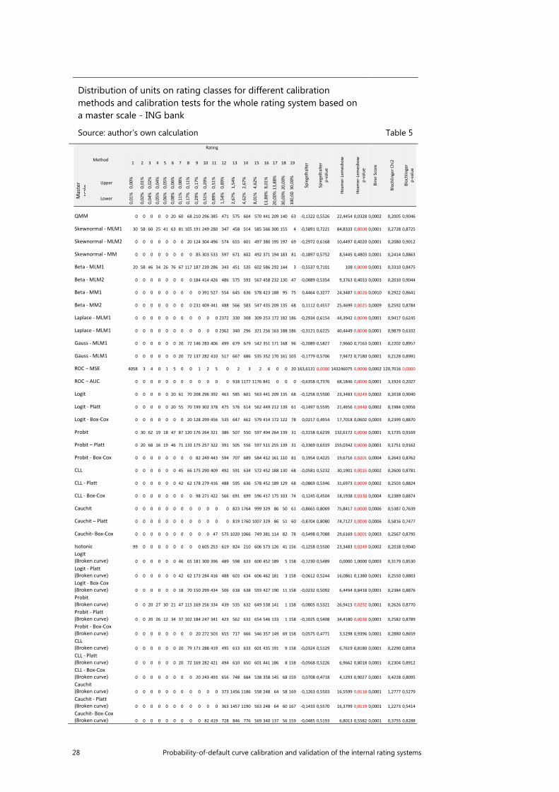
28 Probability-of-default curve calibration and validation of the internal rating systems
Distribution of units on rating classes for different calibration methods and calibration tests for the whole rating system based on a master scale - ING bank
Source: author’s own calculation Table 5
Method
Rating
Spie
gelh
alte
r
Spie
gelh
alte
r p-
valu
e
Hosm
er-L
emes
how
Hosm
er-L
emes
how
p-
valu
e
Bire
r Sco
re
Bloc
hlin
ger C
hi2
Bloc
hlin
ger
p-va
lue
1 2 3 4 5 6 7 8 9 10 11 12 13 14 15 16 17 18 19
Mas
ter
scal
e Upper
0,00
%
0,01
%
0,02
%
0,04
%
0,05
%
0,06
%
0,08
%
0,11
%
0,17
%
0,29
%
0,51
%
0,89
%
1,54
%
2,67
%
4,62
%
8,01
%
13,8
8%
20,0
0%
30,0
0%
Lower
0,01
%
0,02
%
0,04
%
0,05
%
0,06
%
0,08
%
0,11
%
0,17
%
0,29
%
0,51
%
0,89
%
1,54
%
2,67
%
4,62
%
8,01
%
13,8
8%
20,0
0%
30,0
0%
100,
00%
QMM 0 0 0 0 0 20 60 68 210 296 385 471 575 604 570 441 209 140 63 -0,1322 0,5526 22,4454 0,0328 0,0002 0,2005 0,9046
Skewnormal - MLM1 30 58 60 25 41 63 81 105 191 249 280 347 458 514 585 566 300 155 4 -0,5891 0,7221 84,8333 0,0000 0,0001 0,2728 0,8725
Skewnormal - MLM2 0 0 0 0 0 0 0 20 124 304 496 574 655 601 497 380 195 197 69 -0,2972 0,6168 10,4497 0,4020 0,0001 0,2080 0,9012
Skewnormal - MM 0 0 0 0 0 0 0 0 85 303 533 597 671 602 492 371 194 183 81 -0,1897 0,5752 8,5445 0,4803 0,0001 0,2414 0,8863
Beta - MLM1 20 58 46 34 26 76 67 117 187 239 286 343 451 535 602 586 292 144 3 -0,5537 0,7101 108 0,0000 0,0001 0,3310 0,8475
Beta - MLM2 0 0 0 0 0 0 0 0 184 414 426 486 575 593 567 458 232 130 47 -0,0889 0,5354 9,3763 0,4033 0,0003 0,2010 0,9044
Beta - MM1 0 0 0 0 0 0 0 0 0 391 527 554 645 636 578 423 188 95 75 0,4464 0,3277 24,3487 0,0020 0,0010 0,2922 0,8641
Beta - MM2 0 0 0 0 0 0 0 0 231 409 441 488 566 583 547 435 209 135 68 0,1112 0,4557 25,4699 0,0025 0,0009 0,2592 0,8784
Laplace - MLM1 0 0 0 0 0 0 0 0 0 0 0 2372 330 308 309 253 172 182 186 -0,2934 0,6154 44,3942 0,0000 0,0001 0,9417 0,6245
Laplace - MLM1 0 0 0 0 0 0 0 0 0 0 0 2362 340 296 321 256 163 188 186 -0,3121 0,6225 40,4449 0,0000 0,0001 0,9879 0,6102
Gauss - MLM1 0 0 0 0 0 0 20 72 146 283 406 499 679 679 542 351 171 168 96 -0,2089 0,5827 7,9660 0,7163 0,0001 0,2202 0,8957
Gauss - MLM1 0 0 0 0 0 0 20 72 137 282 410 517 667 686 535 352 170 161 103 -0,1779 0,5706 7,9472 0,7180 0,0001 0,2128 0,8991
ROC – MSE 4058 3 4 0 1 5 0 0 1 2 5 0 2 3 2 6 0 0 20 163,6131 0,0000 143246075 0,0000 0,0002 120,7016 0,0000
ROC – AUC 0 0 0 0 0 0 0 0 0 0 0 0 918 1177 1176 841 0 0 0 -0,6358 0,7376 68,1846 0,0000 0,0001 3,1924 0,2027
Logit 0 0 0 0 0 20 61 70 208 296 392 463 585 601 563 441 209 135 68 -0,1258 0,5500 23,3483 0,0249 0,0002 0,2018 0,9040
Logit - Platt 0 0 0 0 0 20 55 70 199 302 378 475 576 614 562 449 212 139 61 -0,1497 0,5595 21,4656 0,0440 0,0002 0,1984 0,9056
Logit - Box-Cox 0 0 0 0 0 0 0 20 128 299 456 535 647 662 579 414 172 122 78 0,0217 0,4914 17,7018 0,0602 0,0003 0,2399 0,8870
Probit 0 30 62 19 18 47 87 120 176 264 321 386 507 550 597 494 264 139 31 -0,3158 0,6239 132,6172 0,0000 0,0001 0,1735 0,9169
Probit – Platt 0 20 68 16 19 46 71 133 175 257 322 391 505 556 597 511 255 139 31 -0,3369 0,6319 155,0342 0,0000 0,0001 0,1751 0,9162
Probit - Box-Cox 0 0 0 0 0 0 0 0 82 249 443 594 707 689 584 412 161 110 81 0,1954 0,4225 19,6716 0,0201 0,0004 0,2643 0,8762
CLL 0 0 0 0 0 0 45 66 175 290 409 492 591 634 572 452 188 130 68 -0,0581 0,5232 30,1901 0,0015 0,0002 0,2600 0,8781
CLL - Platt 0 0 0 0 0 0 42 62 178 279 416 488 595 636 578 452 189 129 68 -0,0869 0,5346 31,6973 0,0009 0,0002 0,2503 0,8824
CLL - Box-Cox 0 0 0 0 0 0 0 0 98 271 422 566 691 699 596 417 175 103 74 0,1245 0,4504 18,1938 0,0330 0,0004 0,2389 0,8874
Cauchit 0 0 0 0 0 0 0 0 0 0 0 0 823 1764 999 329 86 50 61 -0,8665 0,8069 75,8417 0,0000 0,0006 0,5387 0,7639
Cauchit – Platt 0 0 0 0 0 0 0 0 0 0 0 0 819 1760 1007 329 86 51 60 -0,8704 0,8080 74,7127 0,0000 0,0006 0,5816 0,7477
Cauchit- Box-Cox 0 0 0 0 0 0 0 0 0 0 47 575 1020 1066 749 381 114 82 78 -0,5498 0,7088 29,6169 0,0001 0,0003 0,2567 0,8795
Isotonic 99 0 0 0 0 0 0 0 0 605 253 619 824 210 606 573 126 41 156 -0,1258 0,5500 23,3483 0,0249 0,0002 0,2018 0,9040 Logit (Broken curve) 0 0 0 0 0 0 46 65 181 300 396 489 598 633 600 452 189 5 158 -0,1230 0,5489 0,0000 1,0000 0,0003 0,3179 0,8530 Logit - Platt (Broken curve) 0 0 0 0 0 0 42 62 173 284 416 488 603 634 606 462 181 3 158 -0,0612 0,5244 16,0861 0,1380 0,0001 0,2550 0,8803 Logit - Box-Cox (Broken curve) 0 0 0 0 0 0 18 70 150 299 434 506 618 638 593 427 190 11 158 -0,0232 0,5092 6,4494 0,8418 0,0001 0,2384 0,8876 Probit (Broken curve) 0 0 20 27 30 21 47 115 169 256 334 439 535 632 649 538 141 1 158 -0,0805 0,5321 26,9415 0,0292 0,0001 0,2626 0,8770
Probit - Platt (Broken curve) 0 0 20 26 12 34 37 102 184 247 341 423 562 632 654 546 133 1 158 -0,1025 0,5408 34,4180 0,0030 0,0001 0,2582 0,8789 Probit - Box-Cox (Broken curve) 0 0 0 0 0 0 0 0 20 272 503 655 717 666 546 357 149 69 158 0,0575 0,4771 3,5298 0,9396 0,0001 0,2880 0,8659 CLL (Broken curve) 0 0 0 0 0 0 20 79 171 288 419 495 613 633 601 435 191 9 158 -0,0324 0,5129 6,7619 0,8180 0,0001 0,2290 0,8918
CLL - Platt (Broken curve) 0 0 0 0 0 0 20 72 169 282 421 494 610 650 601 441 186 8 158 -0,0568 0,5226 6,9662 0,8018 0,0001 0,2304 0,8912 CLL - Box-Cox (Broken curve) 0 0 0 0 0 0 0 0 20 243 493 656 748 684 538 358 145 68 159 0,0708 0,4718 4,1293 0,9027 0,0001 0,4228 0,8095 Cauchit (Broken curve) 0 0 0 0 0 0 0 0 0 0 0 373 1456 1186 558 248 64 58 169 -0,1263 0,5503 16,5599 0,0110 0,0001 1,2777 0,5279
Cauchit - Platt (Broken curve) 0 0 0 0 0 0 0 0 0 0 0 363 1457 1190 563 248 64 60 167 -0,1433 0,5570 16,3799 0,0119 0,0001 1,2273 0,5414 Cauchit- Box-Cox (Broken curve) 0 0 0 0 0 0 0 0 0 82 419 728 846 776 569 340 137 56 159 -0,0485 0,5193 6,8013 0,5582 0,0001 0,3755 0,8288

Probability-of-default curve calibration and validation of the internal rating systems 29
![Khadirarishta Restrains Lipid Peroxidation in Human ... · PDF filekhadirarishta. [12] A calibration curve was prepared using standard gallic acid. Khadirarishta sample was ... curve](https://img.pdfslide.us/doc/110x75/5ab755be7f8b9a7c5b8eaf39/khadirarishta-restrains-lipid-peroxidation-in-human-12-a-calibration-curve.jpg)