Creating geometrically-correct photo-interpretations ... · PDF fileTechnicalNote:Creatinggeometrically-correctphoto-interpretationsetc. 6 3. Import the scanned map into ILWIS, from

Technical note:Creating geometrically-correct photo-interpretations, photomosaics, andbase maps for a project GIS

D G Rossiter∗, T Hengl†

Soil Science Division, ITC

(Version with figures)3rd Revised Version

26–March–2002

Contents

1 Overview 3

2 Materials 32.1 Physical materials . . . . . . . . . . . . . . . . . . . . . . . . . . . . . . . 32.2 Computer software and datasets . . . . . . . . . . . . . . . . . . . . . . . 4

3 Procedure 43.1 Interpret the airphotos . . . . . . . . . . . . . . . . . . . . . . . . . . . . . 53.2 Make a digital version of the topographic map . . . . . . . . . . . . . . . . 53.3 Select a geo-referencing method . . . . . . . . . . . . . . . . . . . . . . . 73.4 Identify tiepoints . . . . . . . . . . . . . . . . . . . . . . . . . . . . . . . 7

3.4.1 Tiepoints for the photo . . . . . . . . . . . . . . . . . . . . . . . . 83.4.2 Tiepoints for the overlay . . . . . . . . . . . . . . . . . . . . . . . 8

3.5 Prepare for geo-referencing . . . . . . . . . . . . . . . . . . . . . . . . . . 83.5.1 Extra preparation for orthophoto geo-referencing . . . . . . . . . . 9

3.6 Geo-reference . . . . . . . . . . . . . . . . . . . . . . . . . . . . . . . . . 93.6.1 Geo-reference the photos from the topographic map . . . . . . . . 103.6.2 Geo-reference overlays from the photos . . . . . . . . . . . . . . . 11

3.7 Digitize the API . . . . . . . . . . . . . . . . . . . . . . . . . . . . . . . . 123.8 Create a thematic map . . . . . . . . . . . . . . . . . . . . . . . . . . . . 133.9 Resample the photo . . . . . . . . . . . . . . . . . . . . . . . . . . . . . . 133.10 Make a photomosaic . . . . . . . . . . . . . . . . . . . . . . . . . . . . . 14

Appendix 15

∗ [email protected], http://www.itc.nl/˜rossiter† [email protected], http://www.itc.nl/personal/hengl

Copyright c© International Institute for Geo-information Science & Earth Observation(ITC) 2002.

1

Technical Note: Creating geometrically-correct photo-interpretations etc. 2

A Computing maximum relief for the projective transformation 15A.1 Derivation . . . . . . . . . . . . . . . . . . . . . . . . . . . . . . . . . . . 15A.2 Final formula & rule-of-thumb . . . . . . . . . . . . . . . . . . . . . . . . 16A.3 Small-format photographs . . . . . . . . . . . . . . . . . . . . . . . . . . 16

B Conversions for scanning 17B.1 Required resolution . . . . . . . . . . . . . . . . . . . . . . . . . . . . . . 17B.2 File sizes . . . . . . . . . . . . . . . . . . . . . . . . . . . . . . . . . . . 18

C What if some materials are sub-standard? 19C.1 A4 scanner . . . . . . . . . . . . . . . . . . . . . . . . . . . . . . . . . . 19C.2 Poor-quality topographic map . . . . . . . . . . . . . . . . . . . . . . . . 19C.3 Topographic map without overprinted grid . . . . . . . . . . . . . . . . . . 19C.4 Topographic map with unreliable coordinates . . . . . . . . . . . . . . . . 20C.5 Airphoto without fiducial marks . . . . . . . . . . . . . . . . . . . . . . . 20

References 20

4 Figures 21


1 Overview

This note is written for those who want to build a GIS of a relatively small project areafor purposes of natural resources inventory, monitoring, and management. Examples atITC are the group project and the individual final assignment for the professional Masterdegree, and the MSc thesis. All such GIS’s should, if at all possible, include:

— a base map, often referred to as a “topographic” map;

— an airphoto mosaic;

— thematic maps, i.e. polygon, segment, or point maps from air photo interpretation.

— a multispectral satellite image and its products such as false-colour composites;

All of these must be geo-referenced and geometrically-corrected in a common coordi-nate system. In these notes, we do not deal with the satellite images, but instead emphasizethe air photo interpretation (API), which we want to convert to an air photo interpretationmap (APIM). This is most easily accomplished by also producing the digital base map andphotomosaic.

Unrectified stereo-pairs of airphotos are invaluable data sources when a detailed 3D viewof the landscape is required, for example in soil-landscape mapping according to the geo-pedological approach [10]. These stereo-pairs are manually interpreted as uncorrected,unreferenced interpretation overlays1 . These are not geometrically-correct, i.e. do nothave a uniform scale and do not preserve angles, because of the well-known problems oftilt, radial, and relief displacement across the photo, as explained in photogrammetrytexts such as [1, Ch. 2], [5, Ch. 9], and [6, Ch. 4]. They also are not geo-referenced, thatis, their location with respect to a coordinate system is not known2. Finally, most projectareas require more than one photograph; therefore the photo-interpretations and photosfrom adjacent images must be combined to produce maps covering the whole area.

Although the principles explained here can applied with many software packages, these in-structions are specific to the ILWIS GIS, version 3 [4, 7], and assume a working knowledgeof this program. ILWIS is quite suitable for small to medium-sized GIS’s, and is used inmany ITC courses to teach the principles of remote sensing and GIS.

These procedures are all covered in other sources, notably the ILWIS Help and various textsand lecture notes. Our purpose in presenting them yet again is to provide a practical yettheoretically-sound procedure that you can follow step-by-step to produce a high-qualityproduct. We have included many hints based on our own and and our colleagues’ hardexperience.

2 Materials

2.1 Physical materials

• Airphotos, with stereo coverage if needed. Contact prints on high-quality photo-graphic paper are preferable. If you must use a scan or photocopy, use the highestresolution possible to make the scan. A scan of 2400 d.p.i. will give reasonable vi-sual resolution for photo-interpretation; a scan of less than 300 d.p.i. resolution willbe difficult to interpret.

1 Single unrectified photos can also be interpreted monoscopically for cultural features such as roads and build-ings, and for natural features that can be seen monoscopically such as streams.

2 although the flight path and principal points may have been recorded by GPS


• Stable mylar for making interpretation overlays

• An A3 (42x29.7 cm) or larger scanner; note that the smaller dimension must holda standard 23x23 cm airphoto plus enough margin to see the fiducial marks. An A4(29.7x21 cm) scanner is just a bit too small. (See C.1 if this is all you have.)

• A topographic map of the area, with overprinted metric grid and known coordi-nate system. This will be converted to digital form (§3.2). Use as stable a productas possible! The ideal are mylar separates, second best are unfolded prints on stablepaper.

• A precise metric ruler (steel preferred), to measure the fiducial marks for the or-thophoto transformation (§3.3). Not needed for projective or direct linear transfor-mations.

2.2 Computer software and datasets

• The ILWIS v3 computer program [4, 7]. You should know how to find the details ofoperations in the on-line Help.

• A coordinate system object defined in ILWIS v3, covering the study area with adefined projection and datum, corresponding to that of the topographic map.

• In areas with significant relief (§3.3), a raster digital elevation model (DEM) cov-ering the whole area, in the common coordinate system. It doesn’t have to be tooprecise for this purpose, since only the elevations are used, not relief parameterssuch as slope gradient; it can cover a larger area.

The question of how to create a DEM requires its own technical note. The ILWISHelp has extensive information on this. In connection with the present procedure,the important point is that any reasonable DEM will produce acceptable results; re-quirements for terrain modelling are much more strict.

If you have a DEM in a different coordinate system, you will have to re-sample itto the common coordinate system. The georeference (grid size and orientation) doesnot have to match other raster maps for the purposes of this note.

In the DEM’s properties, make sure the Interpolate check box is on (checked).

3 Procedure

The steps you will follow are:

1. Interpret the airphotos (§3.1)

2. Make a digital version of the topographic map (§3.2)

3. Select a geo-referencing method (§3.3)

4. Identify tiepoints (§3.4)

5. Prepare for geo-referencing (§3.5)

6. Geo-reference (§3.6), first the photos from the topographic map, and then the over-lays from the photos

7. Digitize the API (§3.7)

8. Create a thematic map from the overlays (§3.8)


9. Resample the photo to make it a map (§3.9)

10. Make a photomosaic map (§3.10)

It is extremely important to evaluate the quality of a step, before going on to the next one.! →Remember, ‘garbage in, garbage out’ applies to each step of the process.

Remember, always keep a log of everything you do, with system output. That way you canlater write a meaningful metadata description of the datasets you are creating.

3.1 Interpret the airphotos

In this step, you create the information content of the final map, by making an airphotointerpretation (API).

1. Register a stable mylar overlay to the airphoto by tracing the main road and streamnetwork; this provides a number of well-defined photo points, namely road andstream junctions, spread over the photo, and aids in making sure the overlay is ex-actly registered on the photo.

2. Interpret the photos over (almost) the entire area of a central photo, using differentadjacent images for stereo-coverage. Use a pen or pencil width of at least 0.3 mm, toshow up well on the scan. It is not necessary to restrict yourself to the central area of! →a photo; it is more efficient to interpret larger areas of fewer photos, using differentadjacent photos to provide stereo coverage.

The result is a mylar overlay with landscape lines.

This is the step where you are creating information so remember, “garbage in,! →garbage out”. If you have a poor-quality photo-interpretation, you will have a poor-quality map, no matter how good its geometry.

Make sure the outside of the study area is closed (bounding box); there is no need todraw lines to separate photos. Figure 1 shows a single photo (AP) and its interpre-tation overlay (API).

3.2 Make a digital version of the topographic map

The topographic map is the highest-quality geometry available for your project, so youshould take care to make a very accurate conversion to digital form.

1. Scan the topographic map at a high enough resolution to provide accurate locations,typically 300d.p.i., which gives a resolution of ≈ 0.1mm per pixel. Note that thehighest-possible plotting accuracy of a paper map produced by computer methods is0.1mm [9, §3.1.3]; 300 d.p.i. is about 15% finer resolution than this. If the map wasproduced by analogue methods, a 100 d.p.i. scan is sufficient to preserve locationaccuracy, although it will not look good.

If you want to preserve the appearance of the map at large magnifications, you willneed to use a higher scan resolution; see Appendix B for how to determine this.

If the scanner is smaller than the map, you will have to scan in sections of the mapseparately, and georeference each one independently, as if they were separate maps.

2. Make sure the scan is in the uncompressed TIF (Tagged Imaged Format) format;this should be an option your scanner software, or you may need to use a graphicsconversion utility.


3. Import the scanned map into ILWIS, from TIF to raster. This will automatically cre-ate a raster map with the same number of rows & columns as the TIF, with coordinatesystem “unknown”.

4. Create a new georeference (create grf). In the form that appears:

(a) Select the GeoRef method “Tiepoints”

(b) Select the project’s coordinate system mentioned in ‘Materials’ (§2).

(c) Select as the background map the raster file you want to georeference, i.e. thescanned topo map.

The georeference editor will open, with the topographic map displayed as the back-ground. There is a lot of help available from ILWIS here (topic “Georeference Tie-points editor: Functionality”), if you get confused.

5. There is an option in the toolbar for the type of transformation; by default it is affine;this is correct for a geometrically-correct (but not geo-referenced) image such as ascanned topographic map. It only requires three tiepoints, but at least six should beentered to be able to check accuracy.

The affine transformation can adjust scale independently in two axes and can alsocorrect for rotation. These are the only two distortions introduced by a good scanner.The distortions due to the projection are corrected by the definition of the coordinatesystem.

However, the scanner may introduce barrel distortions, because the curvature of the! →lens is not completely corrected at the edges. To correct for this, you can choose thefull second order transformation; it requires six tiepoints, but at least ten should beentered to be able to check accuracy.

6. Use the tiepoint editor to digitize the tiepoints. as grid intersections near the edgesof the map, and enter their real-world coordinates, which are known from the gridlines. Zoom in to find the exact centre of the intersection. In a typical case, the gridline as drawn on the map is 0.3 mm wide, which is about 4 pixels at a 300 d.p.i. scan;find the centre pixel of the intersection. The topo map in Figure 2 shows the cornerof a digital topographic map, with the coordinates clearly shown.

7. After you have entered the minimum number of tiepoints, you will see geographiccoordinates for each new point, i.e. the scanned topographic map is geo-referenced.As you add the extra tiepoints, you will see a realistic measure of the accuracy of thetransformation.

8. You should evaluate the accuracy of the geo-referencing both visually and numeri-cally.

To evaluate visually, add the grid lines as an annotation to the displayed map, ina contrasting colour (e.g. yellow). They should be all exactly in the centre of thegrid lines as drawn on the map. The bottom map in Figure 2 shows the detail of awell-registered grid.

To evaluate numerically, examine the DRow and DCol fields for each point. Theseshould be quite small. They should be equivalent to the maximum location accuracyor less at map scale, i.e. 0.1 mm if the map was produced by fully-automated meansor 0.25 mm if by analogue means. If the scan was at 300 d.p.i., this is within one tofour pixels.


3.3 Select a geo-referencing method

In this step, you decide on the type of geo-referencing you will perform: There are threepossibilities:

Projective : Corrects tilt and radial displacement only; suitable for relatively flat or mono-tonically-sloping areas only; does not require a DEM or fiducial marks. Shouldnot be used if there is significant relief displacement. It is often suitable for small-format photos (taken by a standard small-format “35 mm” camera) even if there issignificant relief, because the radial distances are small on the 24x36 mm negative.

See Appendix A for how to compute the maximum allowable relief displacement; aquick rule of thumb for a map that meets map accuracy standards, from a standardphotogrammetric airphoto, is to divide the photo scale number by 10,000 and thenmultiply by 2.5. For example, the maximum allowable relief displacement on a1:20 000 photo is roughly (20, 000/10, 000) · 2.5 = 5 m.

This also can correct tilt in the landscape (as well as tilt in the aircraft), i.e. a tiltedplain that goes only in one direction.

Direct linear : Corrects tilt, radial, and relief displacement; requires a DEM; does not use fiducialmarks. Use if you can’t find the fiducial marks or don’t know the camera focallength. In our experience, this gives almost equal results to orthophoto if tiepointsare accurate.

Orthophoto : Corrects tilt, radial, and relief displacement; requires a DEM, fiducial marks, andthe camera’s focal length. The camera geometry provides a stable reference framefor the tiepoints, so this should give the highest accuracy.

Affine, second-order and other linear transformations can not correct for radial displace-ment, so they should not be used for airphotos.

For your interest: the technical difference between georeference “orthophoto” and “directlinear” lies in the fact that, for the orthophoto, there is a so-called inner orientation thatcan be calculated by ILWIS from the camera geometry. This establishes the relations onthe photo plane as they existed in the aircraft when the photo was taken; then from thetiepoints, ILWIS can calculate where the camera must have been, and the angle of thephoto plane, in relation to the ground. This allows a very precise reconstruction of theoriginal land surface. In the direct linear georeference, there is no inner orientation, so theprincipal point is unknown. That is, we don’t know what point of the photo was directlyunder the camera. So everything must be calculated from the tiepoints.

3.4 Identify tiepoints

In this step, you identify the points which will be used to geo-reference the photos andoverlays in the following steps. This is usually easiest in two steps:

1. Tiepoints on the topographic map to geo-reference the photos

2. Tiepoints on the photos to geo-reference the overlay

The reason for this is that there is much more detail on the photos than on the topographicmap, so that you have a wide choice of good tiepoints to mark on the overlay. These maybe points which are not clear on the topographic map. Also, they can be marked with muchhigher precision on the photo than on the topographic map.


3.4.1 Tiepoints for the photo

1. On each photo, find at eight to twelve tiepoints, well-distributed (especially towardsthe corner), which you can see also on a topographic base map. Be careful to findpoints that you are fairly sure have not moved, in case the sources are of differentdates. Streams change the courses, roads are rebuilt, etc. Figure 3 shows a well-defined tiepoint (here, a rural church) that is clearly visible on both the photo andtopographic map.

It is very important that the points be well-distributed on the photo in the (X, Y)! →direction.

Do not select points that are close together; they will bias the fit: any error of mea-! →surement will be magnified.

In the case of the direct linear transformation (§3.3), the tiepoints must also be wellspread in the Z (height) direction; they should also not be not coplanar, i.e. on a(tilted) plane. See the ILWIS Help topic “ILWIS objects Georeference Direct Linear”for details.

2. Open the digital topographic map, zoom in to locate each tiepoint, and then readtheir coordinates (E,N) off the screen. This does not have to be so precise, sinceyou will locate them exactly during the actual geo-referencing.

Make a list of the tiepoints on each photo, with their number, approximate coor-dinates, and a sketch and description of what they represent (e.g. ‘middle of roadjunction’, ‘center of road bridge over canal’), so you can find them again on thephoto.

3.4.2 Tiepoints for the overlay

1. On each photo, find at eight to twelve tiepoints, well-distributed (especially towardsthe corner). Any clear point will do. You do not have to use points from the topo-graphic map.

The same cautions about point distribution as mentioned just above apply here as! →well.

2. Register the overlay to the photo, and mark the tiepoints very precisely on the over-lay, with a small circle and a number, so you can find them again on the digitalphoto.

Make a list of the tiepoints on each overlay, with their number and a sketch anddescription of what they represent.

3.5 Prepare for geo-referencing

In this step, you prepare materials to be digitally geo-referenced.

1. Scan the photos at the resolution you want to display in your final photo-mosaic, typ-ically 300 dpi or higher, with the fiducial marks if you intend to use the orthophototransformation. (See Appendix B to compute the required resolution.) Use an A3 orlarger scanner, to cover the entire 25x25 cm area. Store them in the project direc-tory as uncompressed TIF (Tagged Imaged Format) files. Either set the scanner toproduce uncompressed files, or convert the format in an image processing software.ILWIS can not import compressed files.


There is a tradeoff between resolution and size: doubling the scan resolution quadru-ples the file size, and at a certain point it becomes impractical.

2. Scan the overlays; this can be at a a coarser resolution than for the photo, since youwill just need to screen digitize over the displayed scanned overlay; also, you shouldhave drawn the interpretation lines with a line at least 0.3 mm wide. So, 0.2 mm to0.25 mm resolution (150 or 100 dpi) is fine.

3. Import the photos and overlays into ILWIS as explained in §3.2.

3.5.1 Extra preparation for orthophoto geo-referencing

In case you have selected “orthophoto” as your geo-referencing method, you must do somemore preparation.

For each photo:

1. Find out the principal distance (focal length) of the camera; it is ≈ 152mm for astandard photogrammetric camera used in aircraft. The exact distance is calibratedin the factory and is often included in the margin of the photograph.

2. Find and mark the fiducial marks on the photo. These are tiny dots (pinprick size)within a larger dark area, either at the corners or in the middle of the edges of thephoto. They may be hard to see; you may need to use the magnifying stereoscope.

3. Find the principal point on the photo, by connecting the opposite fiducial marksby straight lines, and marking their intersection. This point was directly under thecamera when the photo was taken.

4. Measure the distances (X,Y) from the principal point to the fiducial marks, inactual photo mm, considering the principal point (in the centre of the photo) as(0,0). Therefore, X coordinates to the left of the point, and Y coordinates belowit, are negative. Use as high-quality a ruler as you can find, preferably a stable steelruler, and try to measure to 0.1 mm and even estimate to 0.01 mm (maybe using themagnifying stereoscope).

An example for fiducial marks on the four sides, reading clockwise from the rightmargin, is: (0.08,110.92), (-110.92,-0.92), (0.08,-110.92),

(110.92,0.08) (see Figure 4) .

For each overlay:

1. Register the overlay as in §3.1, and, on the overlay, mark the fiducial marks thatyou just identified on the photo.

3.6 Geo-reference

In this step, you specify the relation between ground coordinates and the raster images(scanned photos and overlays), thereby geo-referencing them. You have to follow this stepfor each photo and each overlay, one at a time.

As explained in §3.4, it is more difficult to geo-reference the photo from the topographicmap than the overlay from the photo, because of the finer detail of the photo. So, you willdo this in two steps:

1. Geo-reference the photos from the topographic map (§3.6.1)

2. Geo-reference the overlays from the photos (§3.6.2)


Make sure the first step has given good results before proceeding! Otherwise your thematic! →map will be useless.

3.6.1 Geo-reference the photos from the topographic map

For each photo separately:

1. Create a new georeference (create grf). In the form that appears:

(a) Select the appropriate GeoRef method: “Tiepoints” for the projective, “Directlinear”, or “Orthophoto”.

(b) Select the project’s coordinate system mentioned in ‘Materials’ (§2).

(c) Select the background map, i.e. the raster file of the photo you want to geo-reference.

2. In case you have selected “direct linear” or “orthophoto”, specify the raster DEM.

3. In case you have selected “orthophoto”, you will also be asked to specify the photogeometry: camera principal distance, and the fiducial marks. Enter them in order,clicking on the photo to specify their row and column in the raster image, and enter-ing their photo coordinates in the dialog box. The ILWIS screen for this is shown inFigure 4.

The georeference editor will then open, with the background map displayed.

4. In case you have selected “tiepoints”, you will notice there is an option in the toolbarfor the type of transformation; by default it is “affine”; change it to “projective”.

5. On the displayed photo, add the grid lines in a fairly dense net (e.g. 1000m). Theywill not be shown at first, because there are not enough points to establish a georef-erence.

6. Open the topographic map in another window.

7. Use the tiepoint editor, click on a tiepoint on the photo, switch to the topographicmap, click on the same point on the topographic map, switch back to the photo, andaccept the point.

8. Once you have enough points, you will see geographic coordinates for each newpoint and the pixel size in real-world units, as well as the grid lines.

The image is now geo-referenced; however, this may not yet be the best transforma-tion, and it can even be very bad, because some points may be in error. This canbe for several reasons: (1) because you didn’t read their coordinates correctly, (2)because you didn’t identify them correctly on the photo, or even (3) because they areincorrectly drawn on the map.

Once you have entered all the points, look at the DRow and DCol fields; they givethe error of each point in pixels. Convert these to map mm, using the scan resolution,to see if they are acceptable. Depending on the map accuracy standard, this should beon the order of 0.25 mm (analogue) or 0.1 mm (digital). For example, if the originalscan was at 300 d.p.i., these correspond to 3 and 1 pixels, respectively.

If some points are much worse than others, try disabling them by marking them“False” and see if the overall error decreases. Go back to the original sources to seeif you made a mistake. This step can take quite some time. Figure 5 shows theILWIS georeference editor in action.


Pay close attention to the displayed grid. Lines should be generally parallel E–W! →and N–S, and perpendicular at the intersections. Squares at the center should be abit larger than those at the corners (because the center was closer to the camera, somore photo area is used to represent the same ground area) and on higher areas. Thegrid will be distorted as it crosses hills and valleys: it is displaced away from theprincipal point in valleys (because these were farther from the camera) and towardsit on hills, with the displacement increasing with relief and towards the corners. Therelief effect is magnified by the radial effect, so that hills and vales are most obviousnear the corners (Figure 6) .

If you see converging grid lines, or a pattern that looks like a tilted plain, you have! →made a serious error in marking one or more tie points, so that the scale in one partof the photo is seriously distorted, thereby affecting the transformation (Figure 7) .

Do not delete points just to make the geo-reference better! As a scientist, you require! →evidence to delete a point. For example, you may infer that a point has moved(stream after a flood, or a re-built road), or than you mis-identified it, or even that theoriginal map was in error. Establish a hierarchy of reliability.

(Hint: If you have a bad geo-reference, try making all the points False and thenturning them on one by one, in order of reliability.)

9. When you have entered all the points, and discarded or adjusted any that are inerror, close the editor; now the image is geo-referenced and associated with the newgeoreference you just created.

Note that the photo has not changed its geometry: it still has the same pixels in the samerows and columns, and it still has variable scale across it (i.e. the pixels represent differentground areas). However, with the information we have specified about the tiepoints, ILWIScan calculate, for each pixel, its true location. So the grid lines which follow a fixed E

or N appear distorted on the uncorrected image, and the length of a grid line betweenintersections are different. In fact it’s the other way around: the grid lines are straight andwith a true scale, and the photo is distorted. Once the image is resampled into a north-oriented map (§3.9, below), the grid lines will be straight and areas in the photo will bedistorted.

3.6.2 Geo-reference overlays from the photos

This follows the same procedure, but should not present any problems of point selection,since they are so clear on the photo.

For each overlay:

1. Create a new geo-reference, with the same type as you used for the correspondingphoto.

2. On the displayed overlay, add the grid lines in a fairly dense net (e.g. 1000m).They will not be shown at first, because there are not enough points to establish ageoreference.

3. Open the corresponding photo (already geo-referenced) in another window.

4. Use the tiepoint editor, click on a tiepoint on the overlay, switch to the photo map,click on the same point on the photo, switch back to the overlay, and accept the point.

5. Once you have enough points, you will see geographic coordinates for each newpoint and the pixel size in real-world units, as well as the grid lines.


Once you have entered all the points, look at the DRow and DCol fields; they givethe error of each point in pixels. Convert these to map mm, using the scan resolution,to see if they are acceptable. Since we are dealing with a hand-drawn overlay, we usethe map accuracy standard of 0.25 mm. If the original scan was at 150 d.p.i. (typicalfor an overlay), this corresponds to 1.5 pixels.

There should really be no problems with this step; any significant error means thatyou did not place the tiepoints precisely enough on the overlay: maybe you did notregister the mylar correctly?

6. When you have entered all the points, and verified the accuracy of the transforma-tion, close the editor; now the image is geo-referenced and associated with the newgeoreference you just created.

Now both photos and overlays are geo-referenced, and should agree with the base topo-graphic map: you finally have the beginnings of a GIS database!

3.7 Digitize the API

Now that you have a geo-referenced overlay, you can create a thematic polygon map. Firstyou will digitize the segments (this step), and then you will create the labels and polygontopology (next step).

The ILWIS Help text refers to this process of on-screen digitizing over a geo-referencedbut uncorrected image (here, the overlay) as monoplotting.

1. Create a new segment file using the project’s coordinate system mentioned in ‘Ma-terials’ (§2).

2. Open the segment editor; display any one of the scanned overlay as the backgroundimage.

3. Set the snap tolerance (under File | Customize ...) to match the precisionof the overlay. This tolerance must be entered in ground coordinates, usually meters.Since your drawing accuracy when making the overlay could not have been higherthan 0.25 mm, convert this to meters and enter the value. For example, at 1:1 50000

this is 12.5 m.

4. Trace the segments from the overlay, using on-screen digitizing.

The line codes are not important unless you want to show the origin of the line or itsfuzziness (another subject . . . ). In the normal case, use one class for all segments.

5. When one overlay is complete, choose another overlay as background image. Youwill see the segments from the first overlay, and an empty space under the presentoverlay.

(Note: you can close and re-open the segment editor at any time during this process;make sure to specify the same segment file.)

6. Trace the segments from this overlay, using on-screen digitizing. When you ap-proach existing segments from adjacent overlays, adjust them manually so that theysnap together. The geometry should be very close if you have correctly geo-referencedeach overlay.

7. Repeat this process for each overlay.

Now you are in the position to check that your geo-reference is in fact correct:


• Display the topographic map, and overlay the digitized segments. Check the seg-ments that should correspond to features on the topographic map, e.g. boundaries ofwater bodies, edges of terraces or valleys, etc. In addition, the general form of thesoil boundaries often follows the landscape (e.g. hilltops, steep hillsides) and can bechecked against the relief as shown by the contour lines.

Figure 9 shows the topographic map, with the digitized segments overlaid. Notehow how well they follow the landscape: for example, small vales in the hilland(seen from the pattern of the contour lines, and the streams) are centred in the cor-responding photo-interpretation unit. This depends on a correct photo-interpretationand then all the geo-referencing steps in this technical note.

If these do not correspond, it means that you have incorrectly geo-referenced eitherthe photo or the overlay.

You now have a single geometrically-correct, geo-referenced file with the polygon bound-aries from all the overlays. There is no further use for the digital overlays.

3.8 Create a thematic map

Now you can create the labels and polygon topology.

1. In case there are any ‘open’ polygons on the outside, close them with a boundingline.

2. In the segment editor, check the segments for dead ends and other errors (File |

Check segments)

3. Create a new point file with a new domain which contains the legend categories,for example, soil-landscape map units.

4. On-screen digitize a label point for each polygon, using the segment map as back-ground; give each point its correct label from the domain you just created (e.g.,soil-landscape code).

5. Polygonize the segment map, using the point file as labels (option Label Points

in the Polygonize command).

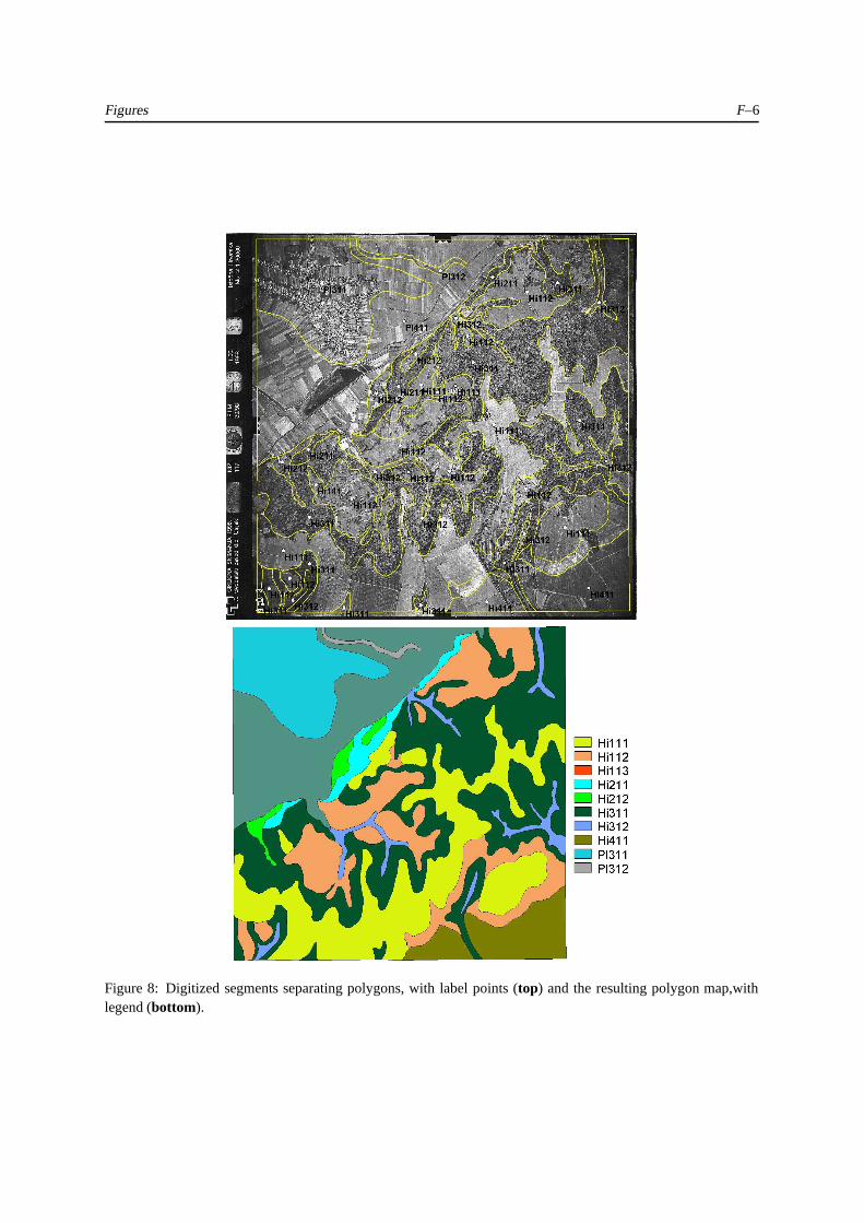
Figure 8 shows the results of on-screen digitizing and a final polygon map.

Now you have a geometrically-correct, geo-referenced polygon map from your photo-interpretation, i.e. you have a thematic map for your GIS. Congratulations!

3.9 Resample the photo

You can convert your set of geo-referenced photos into geometrically-correct, true-scale,north-oriented maps by resampling.

Follow this procedure for each photo; in the next step we will mosaic the resulting maps:

1. Create a new georeference “georeference corners” for the new map.

2. Select the project’s coordinate system mentioned in ‘Materials’ (§2).

3. Specify a pixel size and limiting coordinates (bounding box). You can find the co-ordinates from the limits of the geo-referenced photo. If you want the photo to havethe same resolution as the original, you must determine the pixel size in the geo-referenced image, or you can calculate it approximately from the scan resolution andreported approximate photo scale (see Appendix B).


4. Select operation resample; the input map is the georeferenced photo, the output isa new file, and the georeference is the one you just created.

5. The resulting resampled photo is a north-oriented map. You will notice that it nolonger is square (radial displacement is corrected), and if you used “direct linear”or “orthophoto”, the effect of relief, especially near the corners is obvious. If youoverlay the grid lines,they will be straight and have a true scale.

Figure 10 shows a resampled airphoto, which is now a map.

3.10 Make a photomosaic

You can now make a geometrically-correct, geo-referenced photomosaic from the severalresampled photos. You may be limited by the capacity of your computer; especially if thephotos were scanned with high resolution, you may have to create several photomosaics,each covering a part of your study area.

(If you have access to a workstation with more specialised image processing software (e.g.ERDAS), you may find it easier to export the individual photos to this software, performthe mosaicking and eventual trimming there, and import to ILWIS.)

1. Use operation “Glue Raster Maps” (glueras) to create one mosaic from the sev-eral photos. ILWIS limits you to a maximum of four photos at a time, so you mayhave to build up the final map in pieces.

2. Use operation “SubMap of Raster Map” (subras)) to trim the mosaic to the desiredsize, e.g. if the study area only covers part of the mosaic.

You can also use this to make the photomosaic correspond exactly to the boundariesof topographic map sheets. In this case, you must specify the boundaries as exactcoordinates. If the map series has corners in geographic coordinates, convert these tometric coordinates using the interactive calculator provided by operation “TransformCoordinates” (transform)

Now you have a geometrically-correct, geo-referenced photomosaic of your study area, i.e.you have another map for your GIS. Congratulations!


Appendix

A Computing maximum relief for the projective transformation

See Equation 7 for a quick rule-of-thumb that covers the common case; read the derivationif you are interested in what is really going on.

A.1 Derivation

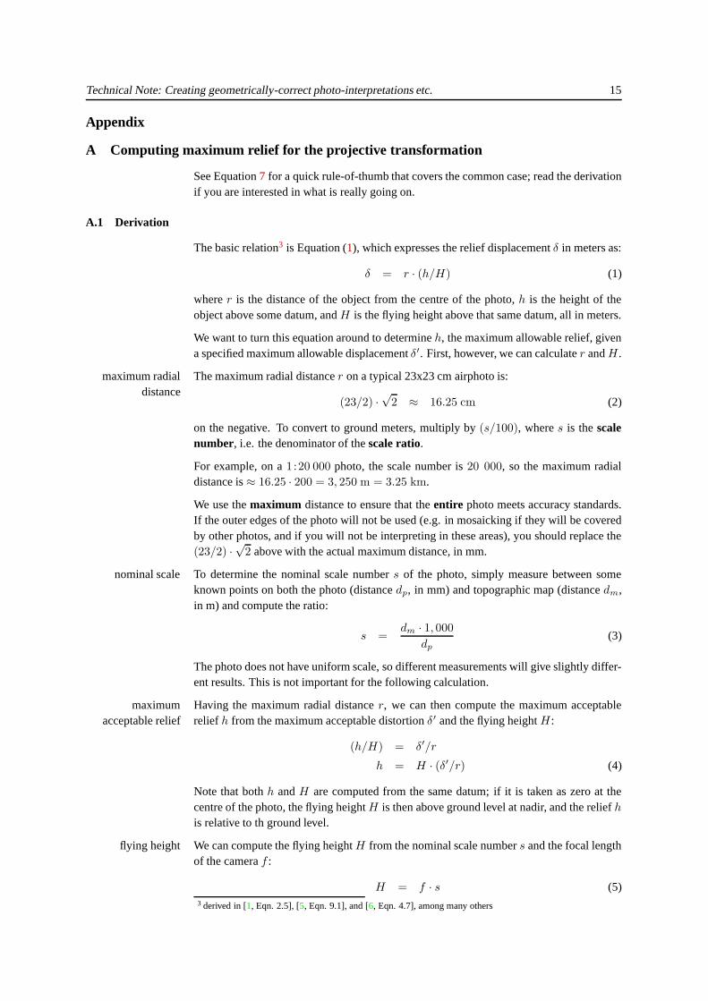
The basic relation3 is Equation (1), which expresses the relief displacement δ in meters as:

δ = r · (h/H) (1)

where r is the distance of the object from the centre of the photo, h is the height of theobject above some datum, and H is the flying height above that same datum, all in meters.

We want to turn this equation around to determine h, the maximum allowable relief, givena specified maximum allowable displacement δ′. First, however, we can calculate r and H .

The maximum radial distance r on a typical 23x23 cm airphoto is:maximum radialdistance

(23/2) ·√

2 ≈ 16.25 cm (2)

on the negative. To convert to ground meters, multiply by (s/100), where s is the scalenumber, i.e. the denominator of the scale ratio.

For example, on a 1:20 000 photo, the scale number is 20 000, so the maximum radialdistance is ≈ 16.25 · 200 = 3, 250 m = 3.25 km.

We use the maximum distance to ensure that the entire photo meets accuracy standards.If the outer edges of the photo will not be used (e.g. in mosaicking if they will be coveredby other photos, and if you will not be interpreting in these areas), you should replace the(23/2) ·

√2 above with the actual maximum distance, in mm.

To determine the nominal scale number s of the photo, simply measure between somenominal scaleknown points on both the photo (distance dp, in mm) and topographic map (distance dm,in m) and compute the ratio:

s =dm · 1, 000

dp

(3)

The photo does not have uniform scale, so different measurements will give slightly differ-ent results. This is not important for the following calculation.

Having the maximum radial distance r, we can then compute the maximum acceptablemaximumacceptable relief relief h from the maximum acceptable distortion δ′ and the flying height H :

(h/H) = δ′/r

h = H · (δ′/r) (4)

Note that both h and H are computed from the same datum; if it is taken as zero at thecentre of the photo, the flying height H is then above ground level at nadir, and the relief h

is relative to th ground level.

We can compute the flying height H from the nominal scale number s and the focal lengthflying heightof the camera f :

H = f · s (5)3 derived in [1, Eqn. 2.5], [5, Eqn. 9.1], and [6, Eqn. 4.7], among many others


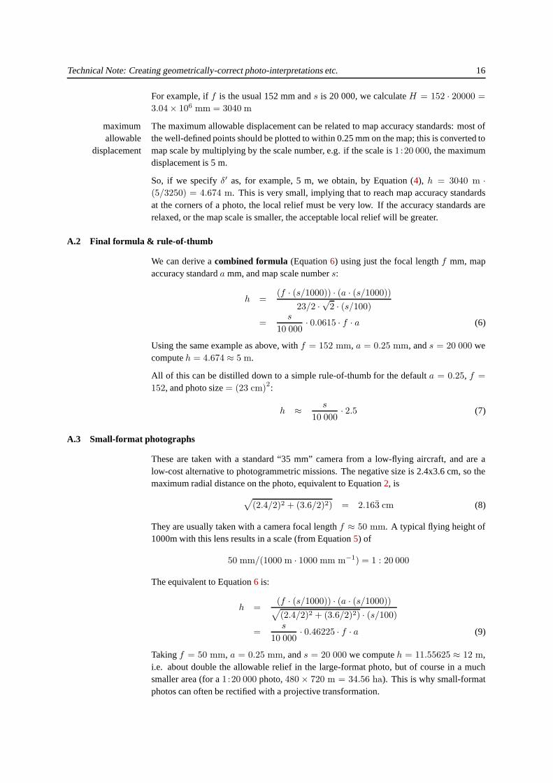
For example, if f is the usual 152 mm and s is 20 000, we calculate H = 152 · 20000 =

3.04× 106 mm = 3040 m

The maximum allowable displacement can be related to map accuracy standards: most ofmaximumallowable

displacementthe well-defined points should be plotted to within 0.25 mm on the map; this is converted tomap scale by multiplying by the scale number, e.g. if the scale is 1:20 000, the maximumdisplacement is 5 m.

So, if we specify δ′ as, for example, 5 m, we obtain, by Equation (4), h = 3040 m ·(5/3250) = 4.674 m. This is very small, implying that to reach map accuracy standardsat the corners of a photo, the local relief must be very low. If the accuracy standards arerelaxed, or the map scale is smaller, the acceptable local relief will be greater.

A.2 Final formula & rule-of-thumb

We can derive a combined formula (Equation 6) using just the focal length f mm, mapaccuracy standard a mm, and map scale number s:

h =(f · (s/1000)) · (a · (s/1000))

23/2 ·√

2 · (s/100)

=s

10 000· 0.0615 · f · a (6)

Using the same example as above, with f = 152 mm, a = 0.25 mm, and s = 20 000 wecompute h = 4.674 ≈ 5 m.

All of this can be distilled down to a simple rule-of-thumb for the default a = 0.25, f =

152, and photo size = (23 cm)2:

h ≈ s

10 000· 2.5 (7)

A.3 Small-format photographs

These are taken with a standard “35 mm” camera from a low-flying aircraft, and are alow-cost alternative to photogrammetric missions. The negative size is 2.4x3.6 cm, so themaximum radial distance on the photo, equivalent to Equation 2, is

√

(2.4/2)2 + (3.6/2)2) = 2.163̄ cm (8)

They are usually taken with a camera focal length f ≈ 50 mm. A typical flying height of1000m with this lens results in a scale (from Equation 5) of

50 mm/(1000 m · 1000 mm m−1) = 1 : 20 000

The equivalent to Equation 6 is:

h =(f · (s/1000)) · (a · (s/1000))

√

(2.4/2)2 + (3.6/2)2) · (s/100)

=s

10 000· 0.46225 · f · a (9)

Taking f = 50 mm, a = 0.25 mm, and s = 20 000 we compute h = 11.55625 ≈ 12 m,i.e. about double the allowable relief in the large-format photo, but of course in a muchsmaller area (for a 1:20 000 photo, 480 × 720 m = 34.56 ha). This is why small-formatphotos can often be rectified with a projective transformation.


All of this can be distilled down to a simple rule-of-thumb for the default a = 0.25 andf = 50:

h ≈ s

10 000· 5.8 (10)

If the flying height is lower or the camera has a longer focal length, the the photo coversless ground area, i.e. scale is larger, and the permissible vertical relief is also larger.

B Conversions for scanning

Conversion for scans, from dots per inch (d.p.i.) to pixels:

100 d.p.i. → 100 pixels in−1

= 100 pixels 25.4 mm−1

= 3.937 pixels mm−1

= 0.254 mm pixel−1 (11)

Common scan resolutions are:

100 d.p.i. → .254 mm pixel−1 (12)

150 d.p.i. → .1693̄ mm pixel−1

300 d.p.i. → .0846̄ mm pixel−1

600 d.p.i. → .0423̄ mm pixel−1

1200 d.p.i. → .02116̄ mm pixel−1

2400 d.p.i. → .010583̄ mm pixel−1

These can be multipled by the map scale number (in thousands) to obtain ground metersper pixel. For example, if a photo’s nominal scale is 1:24 000, and it is scanned at 1200d.p.i., one scan pixel is .02116̄ mm × 50 mm m−1 = 1.0583̄m ≈ 1m

Another way to think about this is the number of pixels per mm:

100 d.p.i. → ≈ 3.94 pixels mm−1 (13)

150 d.p.i. → ≈ 5.91 pixels mm−1

300 d.p.i. → ≈ 11.81 pixels mm−1

600 d.p.i. → ≈ 23.62 pixels mm−1

1200 d.p.i. → ≈ 47.24 pixels mm−1

2400 d.p.i. → ≈ 94.49 pixels mm−1

So to preserve a resolution of, say, 0.1 mm would require a scan of 300 d.p.i.; for fine detailon a topographic map we may want a resolution of 0.01 mm, which requires 2400 d.p.i.

A simple rule-of-thumb to memorize is that 300 d.p.i. corresponds to a pixel size somewhatsmaller than .1 mm.

B.1 Required resolution

There are two requirements: visualisation and location.

The first requirement is æsthetic: you scan at the resolution necessary to preserve the ap-pearance of the original. If it is high-quality, such as a contact photo print or an originalpaper map, very high resolutions are needed. The resolution of silver halide grains in a


contact print on high quality photographic paper is extremely high. For a paper map withhigh-quality paper and printing processess, it is also very high (think of trying to reproducea bank note . . . ).

If the original was produced at a lower resolution (e.g. by printing on a 600 d.p.i. laserprinter), this is the maximum scan resolution; any more is wasted.

However, you may not require such good resolution for your visualisation purposes. Un-less you are going to print at high resolution, it doesn’t make sense to scan at any higherresolution than your final output, allowing of course for any digital enlargement. For ex-ample, if you will print at 300 d.p.i. and you will enlarge by a factor of 2, you would needto scan at 600 d.p.i.

The second requirement depends on the accuracy with which you need to locate points onthe digital product. This is limited by the map scale, both of the source (what is beingscanned) and your final GIS products.

The required location accuracy can not be higher than the working scale of your project,which is typically determined by the accuracy of your base map or GPS receiver, dependingon how you are doing the geo-referencing. In the first case, the limit is set by the mapaccuracy standards [2, Ch. 1], [9, §3.1.3], which for medium- and small-scale maps is0.25 mm on the map if produced by analogue methods and 0.1 mm if produced by fully-automated methods. The 0.25 mm limit can be converted to the scan resolution with theinverse of Eqn. (11), where we see that this is almost exactly equal to 100 d.p.i. In otherwords, a map that conforms to manual accuracy standards should be scanned at 100d.p.i. for purposes of location. The corresponding figure for fully-automated maps is 300d.p.i. These resolutions may not be visually-pleasing, in which case a higher resolutionmay be used.

Note that 0.25 mm on the map corresponds to 12.5m on the ground for a 1:50 000 map,and to 5m for a 1:20 000 map; the corresponding figures of 0.1 mm on the map are 5mand 2m. This implies that location accuracy from printed maps are not particularly high;values such as those for the 0.25 mm accuracy can be obtained with most single-receiverfield GPS; for the 0.1 mm accuracy differential GPS must be used.

B.2 File sizes

Using large scan resolutions leads to file sizes that may not be practical. To determine thestorage requirement, multiply one dimension, in mm, by the number of pixels mm−1; thisgives the number of row or columns. Multiply the dimensions to determine the number ofpixels, and finally by the number of bytes per pixel to determine total storage requirement.

For example, a standard 23x23 cm photo at 300 d.p.i. requires approximately:

23cm × 10mm cm−1 × 11.81 pixels mm−1 = 2, 716 rows

2, 716 rows × 2, 716 columns = 7, 376, 656 pixels

≈ 7.035 Mb

For 600 d.p.i. this is quadrupled to ≈ 28.14 Mb, which is quite large even for today’s(2001 c.e.) Windows-based workstation. At 150 d.p.i. this is reduced to a much moremanageable ≈ 1.76 Mb.


C What if some materials are sub-standard?

It may be that not all the materials listed in §2 are as they should be. In this section we givesome hints for the most common cases.

C.1 A4 scanner

If you can only find an A4 (29.7x21 cm) scanner, you will not be able to fit a standard23x23 cm airphoto plus margins for the fiducial marks, in one dimension.

The best you can do is scan the central 21 cm in one dimension, and use the direct lineartransformation. The marginal areas that you could not scan must be included in scans ofadjacent photos, for the final photo-mosaic. Do not interpret in these areas.

C.2 Poor-quality topographic map

Unfortunately, sometimes one has to work with ripped, worn-out, multiply-folded basemaps, which may even be copies on unstable paper, rather than original prints. In suchcases, it is impossible to geo-reference a scan, since the scale will be far from uniformacross the map.

If the map has an over-printed grid, the solution is to measure the coordinates (E,N) ofthe control points in a local area of the map, using a precise metric ruler (steel preferred).Since the distortion in a small area of the map is relatively small, the coordinates should beadequate.

Especially with photocopies, but also with poor-quality originals, play close attention tothe true scale, which may not match the nominal scale. Use the metric ruler to establishthe true scale in the local area, by measuring the mm between grid lines of known distance.

You should be able to read with a good steel millimeter ruler to .25 mm (map accuracystandard), i.e. 12.5m for 1:50 000 scale maps (since 1 mm = 50m). In practice, this meansyou should divide a 1 mm unit into 4 and read to the nearest 0.25 mm.

For example, if the overprint grid is 1x1km, as is typical, and the actual distance betweengrid lines, measured on the paper map with the metric ruler, is 37.6 mm (3.76 cm), the truescale is 1 × 106/37.6 ≈ 1:26 596.

If the nominal scale (printed on the map) is 1:25 000, we would expect this distance tobe 40 mm (4 cm). This shows that the copying process has shrunk the map by ((40 −37.6)/40 = 6%, which is not uncommon.

Then, when measuring on the map, you must convert the map mm to ground m with theactual scale. Using the example above, if you read 12.25 mm to the right from the gridline for 325000 E, the coordinate is 325 000 + (12.25 × 26.596) ≈ 325315 E (to thenearest meter).

C.3 Topographic map without overprinted grid

In some countries (e.g. India) maps are printed without a grid; however, these usually haveknown coordinates in (latitude and longitude) at the corners of each topographic sheet,because the map series is usually divided according to the geographic grid.

The solution here is to geo-reference in the geographic coordinate system, with the appro-priate projection, and then transform coordinates to a chosen metric grid, e.g. the localUTM zone in a specific datum.


The specific situation of India, as well as the general technique, is dealt with in [8].

C.4 Topographic map with unreliable coordinates

In some countries, e.g. ex-Soviet Union and satellites, the grid is deliberately distorted,and even the corners of the topographic sheet are not reliable.

In this case, the only good solution is to find the tiepoints in the field with a GPS, usingthe same coordinate system. You can use these same tiepoints to geo-reference the scannedtopographic map.

C.5 Airphoto without fiducial marks

As explained in §3.3 (“Selecting a geo-referencing method”), if the photo has no fiducialmarks, you should use the direct linear transformation if there is significant relief, otherwisethe projective transformation.

References

[1] American Society of Photogrammetry. Manual of photogrammetry. American Soci-ety of Photogrammetry, Falls Church, VA, 4th edition, 1980.

[2] T R Forbes, D Rossiter, and A Van Wambeke. Guidelines for evaluating the adequacyof soil resource inventories. SMSS Technical Monograph 4. Cornell University De-partment of Agronomy, Ithaca, NY, 1987 printing edition, 1982.

[3] Tomislav Hengl. Improving soil survey methodology using advanced mapping tech-niques and grid-based modelling. MSc thesis, International Institute for AerospaceSurvey & Earth Sciences (ITC), 2000.

[4] International Institute for Aerospace Survey and Earth Sciences (ITC).ILWIS Academic. On-line document, 30-Nov-2001 2001. URL:http://www.itc.nl/ilwis/.

[5] Lucas L F Janssen and Gerrit C Huurneman, editors. Principles of remote sensing:an introductory textbook. International Institute for Aerospace Survey and Earth Sci-ences (ITC), Enschede, NL, 2nd edition, 2001.

[6] T M. Lillesand and R W. Kiefer. Remote sensing and image interpretation. JohnWiley & Sons, New York, 3rd edition, 1994.

[7] R Nijmeijer, A de Haas, R J J Dost, and P E Budde. ILWIS 3.0 Academic: User’sguide. International Institute for Aerospace Survey and Earth Sciences (ITC), En-schede, NL, 2001.

[8] David G Rossiter. Creating seamless digital maps from Sur-vey of India topographic sheets. GIS India, 7(3), 1998. URL:http://www.itc.nl/~rossiter/docs/GIS_India_7_3.pdf.

[9] David G Rossiter. Lecture Notes : Methodology for Soil Re-source Inventories. ITC Lecture Notes SOL.27. ITC, En-schede, the Netherlands, 2nd revised edition, 2000. URL:http://www.itc.nl/~rossiter/teach/ssm/SSM_LectureNotes2.pdf.

[10] J A Zinck. Physiography & Soils. ITC Lecture Notes SOL.41. ITC, Enschede, theNetherlands, 1988.

http://www.itc.nl/ilwis/

http://www.itc.nl/~rossiter/docs/GIS_India_7_3.pdf

http://www.itc.nl/~rossiter/teach/ssm/SSM_LectureNotes2.pdf


4 Figures

List of Figures

1 An airphoto and its interpretation overlay . . . . . . . . . . . . . . . . . . . . . . . . . . . . . . 1

2 A geo-referenced topographic map . . . . . . . . . . . . . . . . . . . . . . . . . . . . . . . . . . 2

3 A well-defined tiepoint . . . . . . . . . . . . . . . . . . . . . . . . . . . . . . . . . . . . . . . . 3

4 Specifying the fiducial marks . . . . . . . . . . . . . . . . . . . . . . . . . . . . . . . . . . . . . 4

5 Specifying an orthophoto transformation in the ILWIS georeference editor . . . . . . . . . . . . . 4

6 Displacements due to relief . . . . . . . . . . . . . . . . . . . . . . . . . . . . . . . . . . . . . . 5

7 An incorrect geo-reference . . . . . . . . . . . . . . . . . . . . . . . . . . . . . . . . . . . . . . 5

8 Making the polygon map . . . . . . . . . . . . . . . . . . . . . . . . . . . . . . . . . . . . . . . 6

9 Digitized soil boundaries shown on the topographic map . . . . . . . . . . . . . . . . . . . . . . 7

10 The resampled airphoto, as a map . . . . . . . . . . . . . . . . . . . . . . . . . . . . . . . . . . 8

The data used for these figures are from an ITC MSc thesis project [3]; the study area is Osijek-Baranja County,eastern Croatia.

Figures F–1

Figure 1: Top: A single airphoto (AP) and Bottom: its interpretation overlay (API). The camera and aircraftinformation are shown in the left margin of the photo.

Figures F–2

Figure 2: Top: Detail of a 1:1 50000 topographic map, showing the marginal coordinates. The grid intersectionat the lower left, below the label “Kneževi Vinogradi”, has coordinates (6560000E, 5068000N) in thelocal coordinate system used for this map. Bottom: Detail of a geo-referenced topographic map; the grid linesdrawn by ILWIS (fine yellow lines) exactly overlay the grid lines printed on the topographic map (thicker blacklines). Scan resolution was 300 d.p.i., so the pixel resolution is .0846̄; the grid lines are a bit wider than one pixel,so were probably 0.1 mm thick on the original map, equivalent to 5 m on the ground.

Figures F–3

Figure 3: A well-defined tiepoint (here, St Peter’s Church) that is clearly visible on both the photo (top) andtopographic map (bottom). A small yellow circle has been drawn around the church on the photo. Notice thatthe road near the church has been upgraded (smoother curve) since the map was made; however, it is more diffi-cult to move a church! Also note the coordinates in the geo-referenced products; the map was used as reference(6559404E, 5079827N), so the coordinate in the photo (6559428E, 5079829N) was adjusted dur-ing geo-referencing by (+24E, -2N). The highest possible plotting accuracy for the center of the church is12.5 m at this map scale; the observed error is double this. Perhaps the church was plotted too far west on thetopographic map.

Figures F–4

Figure 4: Specifying the fiducial marks in ILWIS; from the number of pixels in the image and the actual photosize in mm, the program was able to calculate the scan resolution.

Figure 5: The ILWIS georeference editor, while specifying the orthophoto transformation. The program was ableto calculate the camera position when the photo was taken (flying height and nadir, i.e. the principal point, whichwas directly under the camera). Note how the grid lines follow the radial and relief displacements.

Figures F–5

Figure 6: Detail of the relief and radial displacements which are corrected by the ortho-photo transformation.These are shown by overlaying north-oriented straight grid lines on the unrectified but geo-referenced photo.

Figure 7: The ILWIS georeference editor, for the orthophoto transformation, with an incorrect geo-reference. Theco-ordinates for the three tiepoints points are too close together; this increases the scale for that part of the photoand gives the effect of tilt.

Figures F–6

Figure 8: Digitized segments separating polygons, with label points (top) and the resulting polygon map,withlegend (bottom).

Figures F–7

Figure 9: Digitized soil boundaries shown on the topographic map. Note how well they follow the landscape.

Figures F–8

Figure 10: The resampled airphoto, as a map. Note that the grid lines are now exactly vertical and horizontal (sothe top of the map is grid North) and they are equally-spaced; the photo has been locally distorted according tothe ortho-correction.

Documents

Creating geometrically-correct photo-interpretations ... · PDF fileTechnicalNote:Creatinggeometrically-correctphoto-interpretationsetc. 6 3. Import the scanned map into ILWIS, from