Embed Size (px)
Citation preview

COURSE SUMMARY
MATH2067: Differential Equations and Vector
Calculus for Engineers
Shane Leviton [Abstract]

1
Contents Ordinary Differential Equations .............................................................................................................. 7
Revision of first year (From MATH1903): ........................................................................................... 7
Exponential growth: ........................................................................................................................ 7
Logistic equation: ............................................................................................................................ 7
First order ODEs .............................................................................................................................. 7
First order linear differential equations: ......................................................................................... 8
Second order ODEs ......................................................................................................................... 9
First order systems: ....................................................................................................................... 12
Second Year ODEs: ............................................................................................................................ 13
First order linear differentiable equation: .................................................................................... 13
2nd order constant coefficient ODE’s ............................................................................................ 13
Non-Homogeneous case: .............................................................................................................. 14
Principle of superposition: ............................................................................................................ 14
Guessing functions: ....................................................................................................................... 14
Variation or Parameters: ................................................................................................................... 15
Functions needed to calculate ...................................................................................................... 15
Wronksian and fundamental solution .............................................................................................. 16
Notes on Wronksian function: ...................................................................................................... 16
Reduction of order: ........................................................................................................................... 16
Euler-Cauchy Equations: ................................................................................................................... 17
Most commonly: ........................................................................................................................... 17
Series Solutions of ODE’s: ................................................................................................................. 18
Techicality: .................................................................................................................................... 18
Notes: ............................................................................................................................................ 20
Method of Frobenius (regular singular points): ................................................................................ 21
Some definitions for Method of Frobenius: ................................................................................. 21
Notes on Frobenius compared to taylor series: ........................................................................... 22
Bessel’s Equation and Bessel Functions: ........................................................................................... 23
Bessel functions: ........................................................................................................................... 23
Radius of convergence: ..................................................................................................................... 24
Partial Differential Equations ................................................................................................................ 25
Boundary-Value Problems and Fourier Series Separation of varaibles for heat equation ............... 25
1 D heat equation: ........................................................................................................................ 25
Solving 1D heat equation: Separation of variables ....................................................................... 26
Fourier Series: (page 34 of notes) ..................................................................................................... 29

2
Complete set of orthogonality relations of sin/cos: ..................................................................... 29
Heat equation with heat flow out of 𝑥 = 𝐿: ..................................................................................... 31
Case 1: 𝑘 = 𝜆2: ............................................................................................................................. 31
Case 2: 𝑘 = 0 ................................................................................................................................ 31
Case 3: 𝑘 = −𝜆2: .......................................................................................................................... 31
Gibbs Phenomenon ........................................................................................................................... 32
Complex Fourier Series: .................................................................................................................... 34
Complex Fourier series for 𝑓(𝑥) ................................................................................................... 34
Sturm-Liouville Eigenvalue problems: .............................................................................................. 35
Regular Sturm Liouville Egienvalue Problems ............................................................................... 36
Sturm Liouville eigenvalue theorems: .......................................................................................... 36
Sturm Liouville theorems: ............................................................................................................. 36
Orthogonality of eigenvlaues: ....................................................................................................... 37
2D heat equation (heat conduction in a plate): ................................................................................ 39
Rectangular plate: ......................................................................................................................... 39
Circular plate: ................................................................................................................................ 39
Inhomogenoeous heat equation: ..................................................................................................... 41
Inhomogeneous boundary conditions: ......................................................................................... 41
+ heat source: ............................................................................................................................... 42
Inhomogeneous example 2:.......................................................................................................... 45
Application of heat equation: Daily and seasonal temperature variations in the earth .................. 46
transforms: ............................................................................................................................................ 48
Rookie example: ................................................................................................................................ 48
Finding inverse Laplace transforms .............................................................................................. 49
Overall picture to solve with Laplace Transforms: ........................................................................... 50
Suddenly heated half space: Solution by Laplace Transforms:......................................................... 50
Error function: ............................................................................................................................... 51
Properties of Laplace transforms: ..................................................................................................... 52
Shift theorem: ............................................................................................................................... 52
Convolution Theorem for Laplace Transforms: ............................................................................ 53
Laplace’s equation: ............................................................................................................................... 57
Comparison of Laplace’s equation to heat equation: ................................................................... 57
Laplaces (2D rectangular domain) .................................................................................................... 57
Laplaces for a circular disk (homogeneous): ..................................................................................... 60
Solving by separation of variables: ............................................................................................... 60
Revision of fluid flow: ....................................................................................................................... 62

3
Conservation of mass (continuity equation):................................................................................ 62
Fourier Transform solution to heat equation: ...................................................................................... 64
Heat equation on infinite domain: .................................................................................................... 64
Fourier integral identity: ............................................................................................................... 66
Dirac delta function: ..................................................................................................................... 67
THE WAVE EQUATION ........................................................................................................................... 68
1D: ..................................................................................................................................................... 68
Solution: ........................................................................................................................................ 68
Vibrations in a non-uniform string .................................................................................................... 69
With function og 𝑐 ........................................................................................................................ 70
Spherical geometry and the wave equation: .................................................................................... 72
Let’s use separation of variables: 𝑢𝑟, 𝜃, 𝜙, 𝑡 = 𝑤𝑟, 𝜃, 𝜙ℎ𝑡 ........................................................... 73
Spherically symmetric waves in 3D ....................................................................................................... 77
VECTOR CALCULUS ................................................................................................................................ 78
Functions of many variables: ............................................................................................................ 78
Vector addition: ............................................................................................................................ 78
Scalar product: .............................................................................................................................. 78
Zero vector: ................................................................................................................................... 78
Basis vectors: ................................................................................................................................. 78
Scalar vector product .................................................................................................................... 78
Norm of vector: ................................................................................................................................. 79
Cauchy-Schwartz inequality: ............................................................................................................. 79
Angle between vectors: .................................................................................................................... 79
Projection vector: .............................................................................................................................. 79
Orthogonal vectors: .......................................................................................................................... 79
Area of parallelogram: .......................................................................................................................... 79
Jacobian matri: .................................................................................................................................. 79
Vector product (volume of parallelepiped) ...................................................................................... 80
Limits and continuity ............................................................................................................................. 80
Sequnces of vectors .......................................................................................................................... 80
Limit laws: ......................................................................................................................................... 80
Open and closed sets: ........................................................................................................................... 81
Interior point ..................................................................................................................................... 81
OPEN N-Ball: ...................................................................................................................................... 81
Open set: ........................................................................................................................................... 81
Functions of several variables ............................................................................................................... 81

4
Function limit rules: ...................................................................................................................... 81
Continuous functions: ....................................................................................................................... 82
Partial derivatives ................................................................................................................................. 82
Tangents to curves: ........................................................................................................................... 83
Tangent surfaces: .............................................................................................................................. 83
General product rules of differentiation: ............................................................................................. 83
Chain rule: ............................................................................................................................................. 83
Level sets : ............................................................................................................................................. 83
Gradient is perpendicular to level set: .................................................................................................. 84
Higher partial derivateies: .................................................................................................................... 84
Hessian matrix of 𝑓 at 𝒂: ....................................................................................................................... 84
Taylor polynomials: ............................................................................................................................... 84
Taylor’s theorem of the second order: ................................................................................................. 85
Jacobian matrix: .................................................................................................................................... 85
Differentiable functions ........................................................................................................................ 85
Maxima and minima ............................................................................................................................. 85
Global max min: ............................................................................................................................ 87
Mutltiple integrals ................................................................................................................................. 88
To calculate: ...................................................................................................................................... 88
Fubini’s therorem:................................................................................................................................. 88
Change of variables ............................................................................................................................... 88
Application: polar coordinates 𝑥, 𝑦 = 𝑟𝑐𝑜𝑠𝜃, 𝑟𝑠𝑖𝑛𝜃 ............................................................................ 89
Triple integrals ...................................................................................................................................... 89
Transformation formula .................................................................................................................... 90
Application: spherical coordinates.................................................................................................... 90
Cylindrical coordinates:..................................................................................................................... 90
Line integrals ......................................................................................................................................... 91
Notation: ........................................................................................................................................... 91
Unit tangent: ..................................................................................................................................... 91
Arc length .......................................................................................................................................... 91
Line integrals of scalar functions ...................................................................................................... 92
Integrals of vector fields ................................................................................................................... 92
Vector fields ...................................................................................................................................... 93
Potential of 𝑓 .................................................................................................................................... 93
Closed vector field: ........................................................................................................................... 94
Curl .................................................................................................................................................... 94

5
Curl in ℝ2: ......................................................................................................................................... 95
Path independence: .......................................................................................................................... 95
Theorem: ........................................................................................................................................... 95
Theorem ............................................................................................................................................ 97
Integral theorems in 2D ........................................................................................................................ 98
Domain and boundary: ..................................................................................................................... 98
Orientation: ....................................................................................................................................... 98
Green’s theorem ............................................................................................................................... 98
Application of green’s theorem: area of domain .......................................................................... 99
Application of green’s theorem: conservative vector fields ......................................................... 99
Stoke’s theorem in ℝ2 in the plane .................................................................................................. 99
circulation:’ ................................................................................................................................... 99
Flux .................................................................................................................................................... 99
Divergence of a function: .................................................................................................................... 100
Triple integrals .................................................................................................................................... 100
Fubini’s theorem for triple integrals: .................................................................................................. 100
Volume: ....................................................................................................................................... 100
Transformation formula in 3D: ....................................................................................................... 101
Eg cylindrical coordinates ............................................................................................................... 101
Eg 2 spherical coordinates: ............................................................................................................. 102
Surface integrals ................................................................................................................................. 103
Definition of surface ....................................................................................................................... 103
Orientation of surfaces and unit normal to surface ....................................................................... 103
6
Unit normal to implicity given surface: ........................................................................................... 104
Special vase of explicit surface: ...................................................................................................... 104
Unit normal to parametric surface ................................................................................................. 104
Calculation of surface integrals: ..................................................................................................... 104
Surface area of domain: .................................................................................................................. 105
Flux across surface: ............................................................................................................................. 105
Flux across graph: ........................................................................................................................... 106
Implicit representation of surfaces ................................................................................................. 106
Integral theorems in 3D: ..................................................................................................................... 106
Simple domain: ............................................................................................................................... 106
Divergence theorem: ...................................................................................................................... 106
Laplace operator: ................................................................................................................................ 107
Product rule: ................................................................................................................................... 107
Green’s first identity ........................................................................................................................... 107
Green’s second identity: ..................................................................................................................... 107
Stokes theorem for surfaces: .............................................................................................................. 107
Application: conservative vector fields in space ............................................................................. 108

7
Ordinary Differential Equations
Revision of first year (From MATH1903): ODE: has an unknown function of one variable and the derivatives of this function
Order= highest derivate
Exponential growth: 𝑑𝑁
𝑑𝑡= 𝑘𝑁
𝑁(𝑡) = 𝑁0𝑒𝑘𝑡
Logistic equation: 𝑑𝑁
𝑑𝑡= 𝑘𝑁(𝑡)(𝑀 − 𝑁(𝑡)) (𝑤𝑖𝑡ℎ max 𝑝𝑜𝑝 𝑀)
First order ODEs
Direction fields: (eg: logistic equation)
𝑒𝑞𝑢𝑖𝑙𝑖𝑏𝑟𝑖𝑎 𝑖𝑓𝑑𝑦
𝑑𝑥= 𝑓(𝑥) = 0
Separable differential equations:
Are in the form:
𝑑𝑦(𝑥)
𝑑𝑥= 𝑓(𝑥)
∴ 𝑦 = 𝐹(𝑥) + 𝐶 (𝑔𝑒𝑛𝑒𝑟𝑎𝑙 𝑠𝑜𝑙𝑢𝑡𝑖𝑜𝑛)
If given particular conditions: eg, (𝑥1, 𝑦1)
∫𝑦
𝑦1
𝑑𝑦 = ∫ 𝑓(𝑥)𝑥
𝑥1
𝑑𝑥
𝑦 = 𝐹(𝑥) + 𝑦1 − 𝐹(𝑥1)
𝑒𝑔:𝑑𝑦
𝑑𝑥= ln 𝑥 , 𝑎𝑛𝑑 (2,4)𝑖𝑠 𝑜𝑛 𝑡ℎ𝑒 𝑔𝑟𝑎𝑝ℎ

8
∫ 𝑑𝑦𝑦
4
Autonomous first order ode 𝑑𝑦
𝑑𝑥= 𝑔(𝑦)
∴𝑑𝑥
𝑑𝑦=
1
𝑔(𝑦) (𝑎𝑠𝑠𝑢𝑚𝑖𝑛𝑔 𝑔(𝑦) ≠ 0)
𝑥 = ∫1
𝑔(𝑦)𝑑𝑦 (𝑎𝑛𝑑 𝑡ℎ𝑒𝑛 𝑔𝑒𝑡 𝑖𝑛 𝑡𝑒𝑟𝑚𝑠 𝑜𝑓 𝑦(𝑥) = 𝑓(𝑥) 𝑖𝑓 𝑝𝑜𝑠𝑠𝑖𝑏𝑙𝑒)
Separable ODE: 𝑑𝑦
𝑑𝑥= 𝑓(𝑥)𝑔(𝑦)
∫𝑑𝑦
𝑔(𝑦)= ∫ 𝑓(𝑥)𝑑𝑥
𝑡ℎ𝑒𝑛 𝐻(𝑦) = 𝑓(𝑥) + 𝐶, 𝑤ℎ𝑒𝑟𝑒 𝐻(𝑦) =1
𝐺(𝑦)
First order linear differential equations: 𝑑𝑦
𝑑𝑥= 𝑎(𝑥) + 𝑏(𝑥)𝑦
Change into: 𝑑𝑦
𝑑𝑥+ 𝑃(𝑥)𝑦 = 𝑄(𝑥)
Multiply by an integrating factor: which has property that 𝑑𝐼
𝑑𝑥= 𝐼(𝑥)𝑃(𝑥)
: 𝐼(𝑥) = 𝑒∫ 𝑃(𝑥)𝑑𝑥
∴𝐼(𝑥)𝑑𝑦
𝑑𝑥+ 𝑃(𝑥)𝑦 𝐼(𝑥) = 𝑄(𝑥)𝐼(𝑥)
∴𝑑𝑦
𝑑𝑥𝐼(𝑥) + 𝑦
𝑑𝐼(𝑥)
𝑑𝑥= 𝑄(𝑥)𝐼(𝑥)
∴𝑑
𝑑𝑥(𝑦𝐼(𝑥)) = 𝑄(𝑥)𝐼(𝑥)
𝑦 =1
𝐼(𝑥)∫ 𝑄(𝑥)𝐼(𝑥)𝑑𝑥
𝑒𝑔:𝑑𝑦
𝑑𝑥+
2𝑦
𝑥=
1
𝑥𝑒𝑥2
𝐼(𝑥) = 𝑒∫ (
2𝑥
)𝑑𝑥= 𝑒2 ln 𝑥 = 𝑥2
∴𝑥2𝑑𝑦
𝑑𝑥+ 2𝑥𝑦 = 𝑥𝑒𝑥2
𝑑
𝑑𝑥(𝑥2𝑦) = 𝑥𝑒𝑥2

9
𝑥2𝑦 =1
2𝑒𝑥2
+ 𝐶
𝑦 =1
2𝑥2𝑒𝑥2
+𝐶
𝑥2
Classifications of ODEs:
- Separable
- Linear
- Separable and linear
- Neither
If neither separable and linear:
Multiply by a transformation variable:
𝑒𝑔 𝑦𝑑𝑦
𝑑𝑥= 𝑒−𝑥 − 𝑦2 (𝑛𝑒𝑖𝑡ℎ𝑒𝑟 𝑠𝑒𝑝𝑎𝑟𝑎𝑏𝑙𝑒 𝑜𝑟 𝑙𝑖𝑛𝑒𝑎𝑟)
𝑙𝑒𝑡 𝑧 = 𝑦2 ∴ 𝑑𝑧 = 2𝑦 𝑑𝑦
∴ 𝑦(
𝑑𝑧2𝑦)
𝑑𝑥= 𝑒−𝑥 − 𝑧
1
2
𝑑𝑧
𝑑𝑥= 𝑒−𝑥 − 𝑧
𝑑𝑧
𝑑𝑥+ 2𝑧 = 2𝑒−𝑥
𝑑
𝑑𝑥(𝑒2𝑥𝑧) = 2∫ 𝑒𝑥 𝑑𝑥
𝑒2𝑥𝑧 = 2𝑒𝑥 + 𝐶
𝑧 = 2𝑒−𝑥 + 𝐶𝑒−2𝑥
∴ 𝑦 = ±√𝑒−𝑥(2 + 𝐶𝑒−𝑥)
𝑜𝑡ℎ𝑒𝑟 𝑠𝑢𝑏𝑠𝑡𝑖𝑡𝑢𝑡𝑖𝑜𝑛𝑒𝑠: 𝑣 =𝑦
𝑥 𝑜𝑟 𝑤 = 𝑥 + 𝑦
Second order ODEs
Form 𝑎𝑦′′ + 𝑏𝑦′ + 𝑐𝑦 = 𝑑
Homogeneous:
𝑃(𝑥)𝑦′′ + 𝑄(𝑥)𝑦′ + 𝑅(𝑥)𝑦 = 0
2nd order linear homologous equations with constant coefficients
𝑎𝑦′′ + 𝑏𝑦′ + 𝑐𝑦 = 0
𝒚 = 𝒆𝒓𝒙
Eg:

10
𝑦′′ − 𝑦′ − 6𝑦 = 0
∴ 𝑎𝑢𝑥𝑖𝑙𝑙𝑎𝑟𝑦 𝑒𝑞𝑢𝑎𝑡𝑖𝑜𝑛:
𝑟2 − 𝑟 − 6 = (𝑟 − 3)(𝑟 + 2) = 0 𝑟 = −3, 2
∴ 𝑦 = 𝐴𝑒−2𝑥 + 𝐵𝑒2𝑥
If auxiliary equation has 2 real distinct roots:
All fine
- If 2 complex roots:
- Eg: 𝑦′′ + 16𝑦 = 0
∴ 𝑟2 + 16 = 0 𝑟 = ±4𝑖
𝑦 = 𝐴𝑒4𝑖𝑥 + 𝐵𝑒−4𝑖𝑥
𝑏𝑢𝑡: 𝑢𝑠𝑖𝑛𝑔 𝑡ℎ𝑎𝑡 𝑒𝑖𝜃 = 𝑐𝑖𝑠𝜃 ∴
∴ 𝑦 = 𝐴𝑐𝑜𝑠(4𝑥) + 𝐵𝑠𝑖𝑛(4𝑥)
Eg 2: 𝑦′′ − 2𝑦′ + 5𝑦 = 0
∴ 𝑟2 − 2𝑟 + 5 = 0
𝑟 = 1 ± 2𝑖
∴ 𝑦(𝑥) = 𝑒𝑥(𝐴𝑐𝑜𝑠(2𝑥) + 𝐵𝑠𝑖𝑛(2𝑥))
1 root:
𝑒𝑔: 𝑦′′ − 6𝑦′ + 9𝑦 = 0
∴ 𝑟2 − 6𝑟 + 9 = 0 (𝑟 − 3)2 = 0 𝑟 = 3
∴ 𝑦(𝑥) = 𝐴𝑒3𝑥 + 𝐵𝑥𝑒3𝑥
2nd order linear non-homogenous differential equations with constant coefficients
Are: 𝑎𝑦′′ + 𝑏𝑦′ + 𝑐𝑦 = 𝐺(𝑥)
Step 1: find homologous solution of
𝑎𝑦′′ + 𝑏𝑦′ + 𝑐𝑦 = 0, 𝑢𝑠𝑖𝑛𝑔 𝑦 = 𝑒𝑟𝑥 𝑚𝑒𝑡ℎ𝑜𝑑 𝑎𝑏𝑜𝑣𝑒
Step 2: (particular solution)
- If polynomial 𝐺(𝑥) = 𝑔0 + ⋯ + 𝑔𝑛𝑥𝑛: use a general polynomial of same degree
- If exponential G(x) = 𝑒𝛼𝑥: use an expoenential of form
𝐾𝑒𝛼𝑥 (𝑤ℎ𝑒𝑟𝑒 𝛼 𝑖𝑠 𝑠𝑎𝑚𝑒 𝑐𝑜𝑒𝑓𝑓𝑖𝑐𝑖𝑒𝑛𝑡 𝑜𝑓 𝑥 𝑖𝑛 𝑒𝑥𝑝𝑜𝑒𝑛𝑡𝑛𝑡𝑖𝑎𝑙), if alpha was the solution to a
homologous solution, use 𝐾𝑥𝛼𝑥
- If G(x) = cos 𝑜𝑟 sin 𝜔𝑡 is trigonometrix (sin or cos): use 𝑦 = 𝐴𝑠𝑖𝑛(𝜔𝑡) + 𝐵𝑠𝑖𝑛(𝜔𝑡)

11
POLYNOMIAL:
𝑦′′ + 2𝑦′ − 3𝑦 = 𝑥2
𝐻𝑂𝑀𝑂𝐿𝑂𝐺𝑂𝑈𝑆 𝑆𝑂𝐿𝑈𝑇𝐼𝑂𝑁: (𝑎𝑏𝑜𝑣𝑒 𝑚𝑒𝑡ℎ𝑜𝑑): 𝑦ℎ = 𝐴𝑒𝑥 + 𝐵𝑒−3𝑥
𝑃𝐴𝑅𝑇𝐼𝐶𝑈𝐿𝐴𝑅: 𝑦𝑝 = 𝐴𝑥2 + 𝐵𝑥 + 𝐶
∴ 2𝑎 + 2(2𝐴𝑥 + 𝐵) − 3(𝐴𝑥2 + 𝐵𝑥 + 𝐶) = 𝑥2
∴ −3𝐴𝑥2 + (4𝐴 − 3𝐵)𝑥 + (2𝐴 + 2𝐵 − 3𝐶) = 𝑥2
𝐴 = −1
3; 𝐵 = −
4
9; 𝐶 = −
14
27
∴ 𝑦 = 𝑦ℎ + 𝑦𝑝
𝑦(𝑥) = −1
3𝑥2 −
4
9𝑥 −
14
27+ 𝐴𝑒𝑥 + 𝐵𝑒−3𝑥
EXPONENTIAL:
𝑦′′ + 4𝑦 = 𝑒3𝑡
∴ 𝑟2 + 4 = 0; 𝑟 = ±2𝑖 ∴ 𝑦ℎ = 𝐴𝑠𝑖𝑛(2𝑡) + 𝐵𝑐𝑜𝑠(2𝑡)
𝑦𝑝 = 𝐾𝑒3𝑡
∴ 𝑒3𝑡(9𝐾 + 4𝑘) = 𝑒3𝑡; 𝐾 =1
13
∴ 𝑦(𝑡) =1
13𝑒3𝑡 + 𝐴𝑐𝑜𝑠(2𝑡) + 𝐵𝑠𝑖𝑛(2𝑡)
EXPONENTIAL 2:
𝑦′′ − 5𝑦′ + 6𝑦 = 𝑒2𝑥
ℎ𝑜𝑚𝑜𝑙𝑜𝑔𝑜𝑢𝑠: 𝑟2 − 5𝑟 + 6 = (𝑟 − 3)(𝑟 − 2) = 0
𝑟 = 2; 3
∴ 𝑦ℎ = 𝐴𝑒2𝑥 + 𝐵𝑒3𝑥
𝑁𝑂𝑇𝐸: 𝑤𝑒 𝑐𝑎𝑛𝑛𝑜𝑡 𝑢𝑠𝑒 𝑦𝑝 = 𝐾𝑒2𝑥𝑛𝑜𝑤, 𝑎𝑠 𝑖𝑡 𝑖𝑠 𝑖𝑛𝑐𝑙𝑢𝑑𝑒𝑑 𝑖𝑛 𝑡ℎ𝑒 ℎ𝑜𝑚𝑜𝑙𝑜𝑔𝑜𝑢𝑠, 𝑤𝑒 𝑛𝑒𝑒𝑑 𝑡𝑜 𝑢𝑠𝑒
𝑦𝑝 = 𝐾𝑥𝑒2𝑘
𝑦′𝑝 = 𝐾(𝑒2𝑥 + 2𝑥𝑒2𝑥); 𝑦𝑝′′ = 𝐾(𝑒2𝑥 + 2(𝑒2𝑥 + 2𝑥𝑒2𝑥)) = 𝐾(3𝑒2𝑥 + 4𝑥𝑒2𝑥)
∴ 𝐾(3𝑒2𝑥 + 4𝑥𝑒2𝑥) − 5𝐾(𝑒2𝑥 + 2𝑥𝑒2𝑥) + 6𝐾𝑥𝑒3𝑥 = 𝑒2𝑥
3𝐾 − 5𝐾 = 1; 𝐾 = −1
∴ 𝑦(𝑥) = 𝐴𝑒2𝑥 + 𝐵𝑒3𝑥 − 𝑥𝑒2𝑥
If there is only 1 root of homologous: use 𝑦𝑝 = 𝐾𝑥2𝑒𝛼𝑥
TRIGONOMETRIC:
𝑥′′(𝑡) + 9𝑥(𝑡) = cos(𝛼𝑡)
𝑥𝑝(𝑡) = 𝐴𝑐𝑜𝑠(𝛼𝑡) + 𝐵𝑠𝑖𝑛(𝛼𝑡)
∴ 𝑥′′ + 9𝑥 = −(𝐴𝛼2 cos(𝛼𝑡) + 𝐵𝛼2 sin(𝛼𝑡)) + 9(𝐴𝑐𝑜𝑠(𝛼𝑡) + 𝐵𝑠𝑖𝑛(𝛼𝑡)) − cos 𝛼𝑡
∴ 𝐴 =1
9 − 𝛼2; 𝐵 = 0
∴ 𝑥 = 𝐴𝑐𝑜𝑠(3𝑡) + 𝐵𝑠𝑖𝑛(3𝑡 +1
9 − 𝛼2cos(𝛼𝑡)

12
First order systems: 𝑑𝑥
𝑑𝑡= 𝑓(𝑥, 𝑦);
𝑑𝑦
𝑑𝑡= 𝑔(𝑥, 𝑦) (𝑒𝑔 𝑝𝑟𝑒𝑑𝑎𝑡𝑜𝑟 𝑝𝑟𝑒𝑦 𝑠𝑦𝑠𝑡𝑒𝑚)
With constant coefficients: 𝑑𝑥
𝑑𝑡= 𝑎𝑥 + 𝑏𝑦
𝑑𝑦
𝑑𝑡= 𝑐𝑥 + 𝑏𝑦
Step 1: differentiate 1 with respect to t
Use simultaneous equations to substitute in 𝑥′𝑜𝑟 𝑦′ and 𝑥 𝑜𝑟 𝑦
Integrate
differentiate 1st solution
substitute
Eg: 𝑥′(𝑡) = 3𝑥 + 𝑦; 𝑦′(𝑡) = 2𝑥 − 4𝑦
∴ 𝑥′′(𝑡) = 3𝑥′(𝑡) + 𝑦′(𝑡); = 3𝑥′ + 2𝑥 − 4𝑦
∴ 𝑥′′(𝑡) − 3𝑥′(𝑡) − 2𝑥(𝑡) = −4𝑦
∴ 𝑥′′(𝑡) − 3𝑥′ − 2𝑥 = −4(𝑥′ − 3𝑥)
𝑥′′(𝑡) + 𝑥′(𝑡) + 10𝑥 = 0
∴ 𝑟2 + 𝑟 + 10 = 0
𝑟 = 𝑒𝑐𝑡
∴ 𝑥 = 𝐴𝑒𝑟1𝑡 + 𝐵𝑒𝑟2𝑡
∴ 𝑥′ = 𝐴𝑟1𝑒𝑟1𝑡 + 𝐵𝑟2𝑒𝑟2𝑡 = 3𝐴𝑒𝑟1𝑡 + 3𝐵𝑒𝑟2𝑡 + 𝑦
𝑦 = 𝐴(𝑟1 − 3)𝑒𝑟1𝑡 + 𝐵(𝑟2 − 3)𝑒𝑟2𝑡
∴ [𝑥(𝑡)
𝑦(𝑡)] =

13
Second Year ODEs:
First order linear differentiable equation: 𝑑𝑦
𝑑𝑥+ 𝑃(𝑥)𝑦 = 𝑄(𝑥)
Integrating factor:
𝐼(𝑥) = 𝑒∫ 𝑃(𝑥)𝑑𝑥:
Eg:
𝑑𝑦
𝑑𝑥+
2
𝑥𝑦 =
1
𝑥𝑒𝑥2
∴ 𝐼(𝑥) = 𝑒∫ (
2𝑥
)𝑑𝑥 = 𝑒2 ln 𝑥 = 𝑥2
∴ 𝑥2𝑑𝑦
𝑑𝑥+ 2𝑥𝑦 = 𝑥𝑒𝑥2
𝑑
𝑑𝑥(𝑥2𝑦) = 𝑥𝑒𝑥2
∴ 𝑥2𝑦 =1
2𝑒𝑥2
+ 𝐶
𝑦(𝑥) =1
𝑥2(
1
2𝑒𝑥2
+ 𝐶)
2nd order constant coefficient ODE’s 𝑑2𝑦
𝑑𝑥2+ 𝑎
𝑑𝑦
𝑑𝑥+ 𝑏𝑦 = 0 (ℎ𝑜𝑚𝑜𝑔𝑒𝑛𝑒𝑜𝑢𝑠)
𝑡𝑟𝑦: 𝑦 = 𝐶𝑒𝜆𝑥
∴ 𝐶𝑒𝑥(𝜆2 + 𝑎𝜆 + 𝑏) = 0
∴ 𝜆 = 𝜆1, 𝜆2
General solution depends on lambda:
Real and distinct lambda:
𝜆1,2 ∈ ℝ (𝑛𝑜𝑡 𝑒𝑞𝑢𝑎𝑙)
𝑦 = 𝐴𝑒𝜆1𝑥 + 𝐵𝑒𝜆2𝑥
Real non-distinct lambda
𝑦 = (𝐴 + 𝐵𝑥)𝑒𝜆2𝑥
Complex lambda
𝜆1,2 = 𝛼 ± 𝑖𝛽
𝑦 = 𝑒𝛼𝑥(𝐴 cos(𝛽𝑥) + 𝐵 sin(𝛽𝑥))
(𝐴, 𝐵 ∈ ℂ)

14
Non-Homogeneous case:
“Method of undetermined coefficients”: (guesswork)
𝑑2𝑦
𝑑𝑥2+ 3
𝑑𝑦
𝑑𝑥+ 2𝑦 = 6𝑥2 + 8:
Homogeneous case:
𝜆1 = −1; 𝜆2 = −2:
𝑦ℎ = 𝐴𝑒−𝑥 + 𝐵𝑒−2𝑥
Particular case:
𝑡𝑟𝑦 𝑦 = 𝐴𝑥2 + 𝐵𝑥 + 𝐶
∴ (2𝐴) + 3(2𝐴𝑥 + 𝐵) + +2(𝐴𝑥2 + 𝐵𝑋 + 𝐶) = 6𝑥2 + 8
∴ 𝐴 = 3; 𝐵 = −9; 𝐶 =29
2
General solution:
𝑦 = 𝐴𝑒−𝑥 + 𝐵𝑒−2𝑥 + 3𝑥2 − 9𝑥 +29
2
Principle of superposition:
Constant:
𝑑2𝑦
𝑑𝑥2+ 𝐴(𝑥)
𝑑𝑦
𝑑𝑥+ 𝐵(𝑥)𝑦 = 0
If 𝑦1, 𝑦2 𝑎𝑟𝑒 𝑠𝑜𝑙𝑢𝑡𝑖𝑜𝑛𝑠
𝑦 = 𝐶1𝑦1 + 𝐶2𝑦2
Is also a solution
Function:
𝑑2𝑦
𝑑𝑥2+ 𝐴(𝑥)
𝑑𝑦
𝑑𝑥+ 𝐵(𝑥)𝑦 = 𝐶(𝑥)
If 𝑦1 satisfies homogeneous equation (from above), and 𝑦2 satisfies inhomogenous: then
Consider:
�̂� = 𝐶𝑦1 + 𝑦2
∴ (𝐶𝑑2𝑦1
𝑑𝑥2+
𝑑2𝑦2
𝑑𝑥2 ) + 𝐴(𝑥) (𝐶𝑑𝑦1
𝑑𝑥+
𝑑𝑦2
𝑑𝑥) + 𝐵(𝑥)(𝐶𝑦1 + 𝑦2) = 0
∴ 𝐶 (𝑑2𝑦1
𝑑𝑥2+
𝐴(𝑥)𝑑𝑦1
𝑑𝑥+ 𝐵(𝑥)𝑦1) +
𝑑2𝑦2
𝑑𝑥2+ 𝐴(𝑥)
𝑑𝑦2
𝑑𝑥+ 𝐵(𝑥)𝑦2 = 𝐶(𝑥)
Guessing functions: - If polynomial 𝐺(𝑥) = 𝑔0 + ⋯ + 𝑔𝑛𝑥𝑛: use a general polynomial of same degree

15
- If exponential 𝐺(𝑥) = 𝑒𝛼𝑥: use an expoenential of form
𝐾𝑒𝛼𝑥 (𝑤ℎ𝑒𝑟𝑒 𝛼 𝑖𝑠 𝑠𝑎𝑚𝑒 𝑐𝑜𝑒𝑓𝑓𝑖𝑐𝑖𝑒𝑛𝑡 𝑜𝑓 𝑥 𝑖𝑛 𝑒𝑥𝑝𝑜𝑒𝑛𝑡𝑛𝑡𝑖𝑎𝑙), if alpha was the solution to a
homologous solution, use 𝐾𝑥𝛼𝑥
- If 𝐺(𝑥) = 𝑐𝑜𝑠 𝑜𝑟 𝑠𝑖𝑛 𝜔𝑡 is trigonometrix (sin or cos): use 𝑦 = 𝐴𝑠𝑖𝑛(𝜔𝑡) + 𝐵𝑠𝑖𝑛(𝜔𝑡)
Variation or Parameters: - Takes the ‘guesswork’ out, but it takes a while.
For:
𝑑2𝑦
𝑑𝑥2+ 𝐴(𝑥)
𝑑𝑦
𝑑𝑥+ 𝐵(𝑥) 𝑦 = 𝑓(𝑥)
If 𝑦1 and 𝑦2 are satisfy the homogenous ODE:
Eg:
𝑦 = 𝐶1(𝑥)𝑦1(𝑥) + 𝐶2(𝑥)𝑦2(𝑥)
Deriving and simplifying by subbing into 𝑑2𝑦
𝑑𝑥2 + 𝐴(𝑥)𝑑𝑦
𝑑𝑥+ 𝐵(𝑥) 𝑦 = 𝑓(𝑥)
We get: 𝐶1′𝑦1
′ + 𝐶2′ 𝑦2
′ = 𝑓(𝑥)
Try:
𝐶1′𝑦1 + 𝐶2
′ 𝑦2 = 0
∴ 𝑤𝑒 𝑛𝑒𝑒𝑑 𝑡𝑜 𝑠𝑜𝑙𝑣𝑒 𝑓𝑜𝑟: 𝐶1′𝑦1 + 𝐶2
′ 𝑦2 = 0
And
Functions needed to calculate
∴ 𝐶1′ = −
𝑓(𝑥)𝑦2
𝑦1𝑦2′ − 𝑦2𝑦1
′ 𝑎𝑛𝑑 𝐶2′ =
𝑓(𝑥)𝑦1
𝑦1𝑦2′ − 𝑦2𝑦1
′
𝑦1𝑦2′ − 𝑦2𝑦1
′ 𝑖𝑠 𝑐𝑎𝑙𝑙𝑒𝑑 𝑡ℎ𝑒 𝑊𝑟𝑜𝑛𝑠𝑘𝑒𝑖𝑛: 𝑊(𝑥)
∴ 𝐶1′ = −
𝑓(𝑥)𝑦1
𝑊(𝑥) ; 𝐶2
′ =𝑓(𝑥)𝑦1
𝑊(𝑥)
Example:
Eg:
𝑑2𝑦
𝑑𝑥2+ 3
𝑑𝑦
𝑑𝑥+ 2𝑦 = 6𝑥2 + 8:
Homogenous: 𝜆2 + 3𝜆 + 2 = 0:
∴ 𝜆 = −1, −2
∴ 𝑦1 = 𝑒−𝑥; 𝑦2 = 𝑒−2𝑥
∴ 𝑊(𝑥) = 𝑦1𝑦2′ − 𝑦2𝑦1
′ = −𝑒−3𝑥

16
∴ 𝐶1′ =
(6𝑥2 + 8)𝑒−2𝑥
−𝑒−3𝑥; 𝐶2
′ = −(6𝑥2 + 8)𝑒−𝑥
−𝑒−3𝑥
…
∴ 𝑦 = 3𝑥2 − 9𝑥 +29
2+ 𝐴𝑒−𝑥 + 𝐵𝑒−2𝑥
Variation of parameters works for all:
𝑑(𝑛)𝑦
𝑑𝑥(𝑛)+ ∑ 𝐴𝑖(𝑥)
𝑛−1
𝑖=0
𝑑(𝑖)𝑦
𝑑𝑥(𝑖)= 𝑓(𝑥)
Wronksian and fundamental solution For any
𝑦′′ + 𝑝(𝑡)𝑦′ + 𝑞(𝑡)𝑦 = 𝑔(𝑡)
Then:
(𝑦1(𝑡0) 𝑦2(𝑡0)
𝑦1′ (𝑡0) 𝑦2
′ (𝑡0)) (
𝐶1
𝐶2) = (
𝑦0
𝑦0)
Which has solutions if: det ((𝑦1(𝑡0) 𝑦2(𝑡0)
𝑦1′ (𝑡0) 𝑦2
′ (𝑡0))) ≠ 0
Notes on Wronksian function: - If 𝑊(𝑥) ≠ 0, then 𝑦1 𝑎𝑛𝑑 𝑦2 are linearly independent
- If 𝑦1, 𝑦2 are linearly dependent, then 𝑊(𝑥) = 0
- BUT: this DOES NOT mean that if 𝑦1 𝑎𝑛𝑑 𝑦2 are linearly independent, then 𝑊(𝑥) ≠ 0
necessarily happens
Reduction of order: Looking to solve variable coefficient linear equations of the form:
𝑑2𝑦
𝑑𝑥2+ 𝑎(𝑥)
𝑑𝑦
𝑑𝑥+ 𝑏(𝑥)𝑦 = {
0 (ℎ𝑜𝑚𝑜𝑔𝑒𝑛𝑒𝑜𝑢𝑠)
𝑓(𝑥) (𝑖𝑛ℎ𝑜𝑚𝑜𝑔𝑒𝑛𝑒𝑜𝑢𝑠)
Now that we have variation of parameters, we can just look at the homogeneous case, and then
apply variation of parameters to find the inhomogeneous
EG: if the function 𝑢(𝑥) is a solution to 𝑑2𝑦
𝑑𝑥2 + 𝑎(𝑥)𝑑𝑦
𝑑𝑥+ 𝑏(𝑥)𝑦 = 0; try the function
𝑦 = 𝑢(𝑥)𝑣(𝑥)
∴ 𝑦′ = 𝑢𝑣′ + 𝑣′𝑢
𝑦′′ = 𝑢𝑣′′ + 2𝑢′𝑣′ + 𝑣𝑢′′

17
∴ (𝑢𝑣′′ + 2𝑢′𝑣′ + 𝑣𝑢′′) + 𝑎(𝑥)(𝑢𝑣′ + 𝑣′𝑢) + 𝑏(𝑥)(𝑢𝑣) = 0
𝑣(𝑢′′ + 𝑎𝑢′ + 𝑏𝑢) + 𝑢𝑣′′ + (2𝑢′ + 𝑎𝑢)𝑣′ = 0
𝑎𝑠 𝑢 𝑠𝑜𝑙𝑣𝑒𝑠 𝑡ℎ𝑒 𝑂𝐷𝐸: 𝑢′′ + 𝑎𝑢′ + 𝑏𝑢 = 0 ∴ 𝑡ℎ𝑖𝑠 𝑠𝑖𝑚𝑝𝑙𝑖𝑓𝑖𝑒𝑠 𝑡𝑜:
∴𝑣′′
𝑣′= − (𝑎 +
2𝑢′
𝑢)
Then integrate: exponentiate ect
Eg: reduction of order
solve (1 + 𝑥)𝑦′′ + 𝑥𝑦′ − 𝑦 = 0; given 𝑦 = 𝑥 is a solution:
𝑇𝑟𝑦 𝑦 = 𝑥𝑣(𝑥)
∴ 𝑦′ = 𝑥𝑣′ + 𝑣
𝑦′′ = 𝑥𝑣′′ + 2𝑣′
∴ (1 + 𝑥)(𝑥𝑣′′ + 2𝑣′) + 𝑥(𝑥𝑣′ + 𝑣) − 𝑥𝑣 = 𝑣′′(𝑥 + 𝑥2) + 𝑣′(2 + 2𝑥 + 𝑥2) = 0
𝑣′′
𝑣′= − (
𝑥2 + 2𝑥 + 2
𝑥2 + 𝑥) = − (1 +
𝑥 + 2
𝑥2 + 𝑥) = (−1 −
2
𝑥+
1
1 + 𝑥)
∴ ln 𝑣′ = −𝑥 − 2 ln 𝑥 + ln(1 + 𝑥) + �̂�
= ln (𝐶̅(1 + 𝑥)𝑒−𝑥
𝑥2 )
𝑣′ =𝐶̅(1 + 𝑥)𝑒−𝑥
𝑥2
∴ 𝑣 = ∫ 𝐶̅𝑑
𝑑𝑥(
𝑒−𝑥
𝑥)
𝑣 =𝐶𝑒−𝑥
𝑥+ 𝐷
∴ 𝐺𝑒𝑛𝑒𝑟𝑎𝑙 𝑠𝑜𝑙𝑢𝑡𝑖𝑜𝑛: 𝑦 = 𝑥𝑣 = 𝐶𝑒−𝑥 + 𝐷𝑥
Euler-Cauchy Equations: Are of the form:
∑ 𝑎𝑝𝑥𝑝𝑑(𝑝)𝑦
𝑑𝑥(𝑝)
𝑛
𝑝=0
= {0
𝑓(𝑥)
Most commonly:
𝑥2𝑑2𝑦
𝑑𝑥2+ 𝑎𝑥
𝑑𝑦
𝑑𝑥+ 𝑏𝑦 = 0
(can solve = 𝑓(𝑥) with variation of parameters)
Try:
𝑦 = 𝑘𝑥𝜆
∴ 𝑥2(𝑘𝜆(𝜆 − 1)𝑥𝜆−2) + 𝑎𝑥(𝜆𝑘𝑥𝜆−1) + 𝑏(𝑘𝑥𝜆) = 0
𝐴𝑠𝑠𝑢𝑚𝑖𝑛𝑔 𝑙 ≠ 0; 𝑥 ≠ 0 (𝑡𝑟𝑖𝑣𝑖𝑎𝑙 𝑠𝑜𝑙𝑢𝑡𝑖𝑜𝑛)
𝜆(𝜆 − 1) + 𝑎𝜆 + 𝑏 = 𝜆2 + (𝑎 − 1)𝜆 + 𝑏 = 0

18
∴ 𝜆1,2 =(1 − 𝑎 ± √(𝑎 − 1)2 − 4𝑏)
2
Real, distinct lambda:
If 𝜆1, 𝜆2 𝑑𝑖𝑠𝑡𝑖𝑛𝑐𝑡 𝑖𝑛 ℝ:
𝑦 = 𝐴𝑥𝜆1 + 𝐵𝑥𝜆2
Distinct, complex lambda:
𝜆1 ≠ 𝜆2 ∈ ℝ
∴ 𝜆 = 𝛼 ± 𝑖𝛽
∴ 𝑦 = 𝐴𝑥𝛼+𝑖𝛽 + 𝐵𝑥𝛼−𝑖𝛽 = 𝑥𝛼 (𝐴(𝑒ln 𝑥)𝑖𝛽
+ 𝐵(𝑒ln 𝑥)−𝑖𝛽
)
𝑦 = 𝑥𝛼(𝐴 cos(ln 𝛽𝑥) + 𝐵 sin(ln 𝛽𝑥))
(where 𝐴, 𝐵 ∈ ℂ)
Equal roots:
If 𝜆1 = 𝜆2 = 𝜆
𝑦 = 𝐴𝑥𝜆 + 𝐵𝑥𝜆 ln 𝑥
Example of E-C equation:
Solve 𝑥2 𝑑2𝑦
𝑑𝑥2 − 5𝑥𝑑𝑦
𝑑𝑥+ 10 𝑦 = 0
𝑇𝑟𝑦 𝑦 = 𝑘𝑥𝜆
∴ 𝜆(𝜆 − 1) − 5𝜆 + 10 = 𝜆2 − 6𝜆 + 10 = 0
∴ 𝜆 =6 ± √36 − 40
2= 3 ± 𝑖
∴ 𝑆𝑜𝑙𝑢𝑡𝑖𝑜𝑛 𝑖𝑠: 𝑦 = 𝑥3(𝐴 cos(ln 𝑥) + 𝐵 sin(ln 𝑥))
Series Solutions of ODE’s: Uses the Tayloer series:
𝑦 = ∑ 𝑐𝑛𝑥𝑛
∞
𝑛=0
(𝑇𝑎𝑦𝑙𝑜𝑟 𝑆𝑒𝑟𝑖𝑒𝑠 𝑎𝑏𝑜𝑢𝑡 𝑜𝑟𝑖𝑔𝑖𝑛, 𝑠𝑜𝑚𝑒𝑡𝑖𝑚𝑒𝑠 𝑠𝑜𝑚𝑒𝑤ℎ𝑒𝑟𝑒 𝑒𝑙𝑠𝑒)
Techicality: If the series converges uniformly, the series can be differentiated term by term. (This will be
assumed in this course).
Eg:

19
Find the general solution of:
𝑦′′ + 𝑥𝑦′ + 𝑦 = 0:
Let:
𝑦 = ∑ 𝑐𝑛𝑥𝑛
∞
𝑛=0
𝑦′ = ∑ 𝑛 𝑐𝑛𝑥𝑛−1
∞
𝑛=0
= ∑ 𝑛 𝑐𝑛𝑥𝑛−1
∞
𝑛=1
𝑦′′ = ∑ 𝑛(𝑛 − 1)𝑐𝑛𝑥𝑛−2
∞
𝑛=0
= ∑ 𝑛(𝑛 − 1)𝑐𝑛𝑥𝑛−2
∞
𝑛=2
∴ ∑ 𝑛(𝑛 − 1)𝑐𝑛𝑥𝑛−2
∞
𝑛=2
+ 𝑥 ∑ 𝑛 𝑐𝑛𝑥𝑛−1
∞
𝑛=1
+ ∑ 𝑐𝑛𝑥𝑛
∞
𝑛=0
= 0
Shifting indicies, so we can equate powers of 𝑥:
∴ ∑(𝑛 + 2)(𝑛 + 1)𝑐𝑛+2𝑥𝑛
∞
𝑛=0
+ ∑ 𝑛 𝑐𝑛𝑥𝑛−1
∞
𝑛=1
+ ∑ 𝑐𝑛𝑥𝑛
∞
𝑛=0
= 0
→ 2𝑐2 + 𝑐0 + ∑((𝑛 + 2)(𝑛 + 1)𝑐𝑛+2 + (𝑛 + 1)𝑐𝑛)𝑥𝑛
∞
𝑛=1
= 0
(𝑡ℎ𝑒 2𝑐2 𝑎𝑛𝑑 𝑐0 𝑎𝑟𝑒 𝑐𝑜𝑛𝑠𝑡𝑎𝑛𝑡 𝑡𝑒𝑟𝑚𝑠 𝑓𝑟𝑜𝑚 𝑡ℎ𝑒 𝑠𝑢𝑚′𝑠 𝑠𝑡𝑎𝑟𝑡𝑖𝑛𝑔 𝑎𝑡 𝑛 = 0)
∴ 𝑎𝑠 𝑒𝑎𝑐ℎ 𝑝𝑜𝑤𝑒𝑟 𝑜𝑓 𝑥 𝑚𝑢𝑠𝑡 = 0:
2𝑐2 + 𝑐0 = 0 ⟹ 𝑐2 = −𝑐0
2
𝑎𝑛𝑑 𝐶𝑜𝑒𝑓𝑓𝑖𝑐𝑖𝑒𝑛𝑡 𝑥𝑛 = 0:
𝑐𝑛+2 = −(𝑛 + 1)𝑐𝑛
(𝑛 + 2)(𝑛 + 1)= −
𝑐𝑛
𝑛 + 2
∴ 𝑐0 𝑎𝑛𝑑 𝑐1 𝑎𝑟𝑒 𝑎𝑟𝑏𝑖𝑡𝑟𝑎𝑟𝑦; 𝑠𝑜 𝑜𝑑𝑑 𝑑𝑒𝑝𝑒𝑛𝑑 𝑜𝑛 𝑐1, 𝑒𝑣𝑒𝑛 𝑜𝑛 𝑐0
∴ 𝑦 = ∑ 𝑐𝑛𝑥𝑛
∞
𝑛=0
= 𝑐0 + 𝑐1𝑥 + 𝑐2𝑥2 + ⋯
𝑐2 = −𝑐0
2; 𝑐4 = −
𝑐2
4=
𝑐0
8…
𝑐3 = −𝑐1
3; 𝑐5 = −
𝑐3
5=
𝑐1
15…
𝑦(0) = 𝑐0; 𝑦′(0) = 𝑐1
Hence:
𝑦 = 𝑐0 (1 −𝑥2
2+
1
8𝑥4 − ⋯ ) + 𝑐1 (𝑥 −
1
3𝑥3 + ⋯ )

20
= 𝑦(0) (1 −𝑥2
2+
1
8𝑥4 − ⋯ ) + 𝑦′(0) (𝑥 −
1
3𝑥3 + ⋯ )
𝑛𝑜𝑡𝑒: (1 −𝑥2
2+
1
8𝑥4 − ⋯ ) = 𝑒−
𝑥2
2
Now we use reduction of order to find what (𝑥 −1
3𝑥3 + ⋯ )
∴ 𝑙𝑒𝑡 𝑦 = 𝑒−𝑥2
2 𝑣(𝑥) → 𝑦′ = 𝑒−𝑥2
2 (𝑣′ − 𝑣𝑥)
∴ 𝑆𝐼𝑚𝑝𝑙𝑖𝑓𝑦𝑖𝑛𝑔 𝑎𝑛𝑑 𝑠𝑢𝑏𝑏𝑖𝑛𝑔 𝑎𝑛𝑑 𝑡ℎ𝑖𝑛𝑔𝑠:
𝑣′′ − 𝑥𝑣′ = 0
𝑣′′
𝑣′= 𝑥
ln 𝑣′ =𝑥2
2+ 𝐴1
𝑣′ = 𝐴2𝑒−𝑥2
2
𝑣 = 𝐴2 ∫ 𝑒−𝑥2
2 𝑑𝑥
∴ 2𝑛𝑑 𝑠𝑜𝑙𝑢𝑡𝑖𝑜𝑛 𝑚𝑒𝑎𝑛𝑠 𝑡ℎ𝑎𝑡 (𝑥 −1
3𝑥3 + ⋯ ) = 𝑒−
𝑥2
2 ∫ 𝑒−𝑥2
2 𝑑𝑥
∴ 𝑦 = 𝐴𝑒−𝑥2
2 (𝑒−𝑥2
2 ∫ 𝑒−𝑥2
2 𝑑𝑥) = 𝐴𝑒−𝑥2∫ 𝑒−
𝑥2
2 𝑑𝑥
Notes: - You want the series to converge to truly consider it a representation of the solution.
(divergent in another course)
Ratio test for convergence:
𝑓𝑜𝑟 𝑦 = ∑ 𝑐𝑛𝑡𝑛
∞
𝑛=0
:
𝐿 = lim𝑛→∞
|𝑐𝑛+1𝑡𝑛+1
𝑐𝑛𝑡𝑛| = lim
𝑛→∞|𝑐𝑛+1
𝑐𝑛| |𝑡|
𝑖𝑓 𝐿 < 1: 𝑐𝑜𝑛𝑣𝑒𝑟𝑔𝑒𝑠
𝐿 > 1: 𝑑𝑖𝑣𝑒𝑟𝑔𝑒𝑠
𝐿 = 1: 𝑛𝑜𝑡 𝑒𝑛𝑜𝑢𝑔ℎ 𝑖𝑛𝑓𝑜

21
This technique will work for any 𝑎(𝑥)𝑎𝑛𝑑 𝑏(𝑥) themselves admit converging Taylor series
expansions at 𝑥 = 0; convergent with some radius |𝑥| < 𝑅
Method of Frobenius (regular singular points):
Some definitions for Method of Frobenius: If 𝑦′′ + 𝑃(𝑥)𝑦′ + 𝑄(𝑥)𝑦 = 0:
- If 𝑃(𝑥)𝑎𝑛𝑑 𝑄(𝑥) remain finite at 𝑥 = 𝑥0, 𝑥0 is called an ordinary point
- If either 𝑃(𝑥) or 𝑄(𝑋) divereges as 𝑥 → 𝑥0, then 𝑥0 is called a singular point
- If either 𝑃(𝑥) or 𝑄(𝑥) diverges as 𝑥 → 𝑥0, but (𝑥 − 𝑥0)𝑃(𝑥) and (𝑥 − 𝑥0)2𝑄(𝑥) remains
finite as 𝑥 → 𝑥0, 𝑥 = 𝑥0 is a regular singular point
Consider (note: singularity at 𝑥 = 0) :
𝑦′′ +𝛼(𝑥)
𝑥𝑦′ +
𝛽(𝑥)
𝑥2𝑦 = 0
∴ 𝑡𝑖𝑚𝑒𝑠 𝑏𝑦 𝑥2
(𝑥 = 0 is a regular singular point)
NOW: seek solutions of the form:
𝑦 = 𝑥𝑟 ∑ 𝑐𝑛𝑥𝑛
∞
𝑛=0
= ∑ 𝑐𝑛𝑥𝑛+𝑟
∞
𝑛=0
𝑒𝑥𝑎𝑚𝑝𝑙𝑒:
2𝑥2𝑦′′ − 𝑥𝑦′ + (1 + 𝑥)𝑦 = 0
𝑐0 ≠ 0; 𝑥 > 0
→ 𝑦′ = ∑(𝑛 + 𝑟)𝑐𝑛𝑥𝑛+𝑟−1
∞
𝑛=0
; 𝑦′′ = ∑(𝑛 + 𝑟)(𝑛 + 𝑟 − 1)𝑐𝑛𝑥𝑛+𝑟−2
∞
𝑛=0
∴ 2 ∑ 𝑐𝑛(𝑛 + 𝑟)(𝑛 + 𝑟 − 1)𝑥𝑛+𝑟
∞
𝑛=0
− ∑ 𝑐𝑛(𝑛 + 𝑟)𝑥𝑛+𝑟
∞
𝑛=0
+ (1 + 𝑥) ∑ 𝑐𝑛𝑥𝑛+𝑟
∞
𝑛=0
= 0
∴ ∑ 𝑐𝑛[(2𝑛 + 2𝑟 − 1)(𝑛 + 𝑟 − 1)]𝑥𝑛+𝑟
∞
𝑛=0
+ ∑ 𝑐𝑛𝑥𝑛+𝑟+1
∞
𝑛=0
= 0
∴ 𝑥𝑟 {(2𝑟 − 1)(𝑟 − 1)𝑐0 + ∑(𝑐𝑛(2𝑛 + 2𝑟 − 1)(𝑛 + 𝑟 − 1) + 𝑐𝑛−1)𝑥𝑛)
∞
𝑛=1
} = 0
Radius of convergence
The lowest power is 𝑥𝑟, which gives a solution of 𝑟 =1
2, 1

22
∴ 𝑐𝑛(2𝑛 + 2𝑟 − 1)(𝑛 + 𝑟 − 1) + 𝑐𝑛−1 = 0
∴ 𝑐𝑛 = −𝑐𝑛−1
(𝑛 + 𝑟 − 1)(2𝑛 + 2𝑟 − 1)
For 𝑟 = 1:
𝑐𝑛 = −𝑐𝑛−1
𝑛(2𝑛 + 1)
∴ 𝑦1 = 𝑐0𝑥(1 −1
1 × 3𝑥 +
1
2 × 3 × 5𝑥3 − (
1
1 × 2 × 3 × 5 × 7) 𝑥3 + ⋯ )
For 𝑟 =1
2:
𝑐𝑛 = −𝑐𝑛−1
𝑛(2𝑛 − 1)
∴ 𝑐1 = −𝑐0; 𝑐2 = −𝑐1
3 ∙ 2=
𝑐0
2 × 3;
∴ 𝑦2 = 𝑐0𝑥12 (1 − 𝑥 +
1
6𝑥2 + ⋯ )
∴ 𝐺𝑒𝑛𝑒𝑟𝑎𝑙 𝑠𝑜𝑙𝑢𝑡𝑖𝑜𝑛 𝑡𝑜 2𝑥2𝑦′′ − 𝑥𝑦′ + (1 + 𝑥)𝑦 = 0 𝑖𝑠:
𝑦 = 𝐴𝑥 (1 −1
1 ∙ 3𝑥 + ⋯ ) + 𝐵𝑥
12(1 − 𝑥 + ⋯ )
Radius of convergence:
For 𝑟 = 1: 𝑐𝑛 = −𝑐𝑛−1
𝑛(2𝑛+1)
∴ lim𝑛→∞
|𝑐𝑛𝑥𝑛
𝑐𝑛−1𝑥𝑛−1| = lim𝑛→∞
(|−𝑐𝑛−1
𝑛(2𝑛 + 1)𝑐𝑛−1| |𝑥|)
= lim𝑛→∞
(|−1
2𝑛2 + 𝑛| |𝑥|) → 0 < 1
∴ 𝑅 → ∞
For 𝑟 =1
2: 𝑐𝑛 = −
𝑐𝑛−1
𝑛(2𝑛−1)
∴ lim𝑛→∞
|𝑐𝑛𝑥𝑛
𝑐𝑛−1𝑥𝑛−1| = lim𝑛→∞
(|−𝑐𝑛−1
𝑛(2𝑛 − 1)𝑐𝑛−1| |𝑥|)
= lim𝑛→∞
(|−1
2𝑛2 − 1| |𝑥|) → 0 < 1
∴ 𝑅 → ∞
Notes on Frobenius compared to taylor series: Not: for frobenius, as 𝑦 = ∑ 𝑐𝑛𝑥𝑛+𝑟∞
𝑛=0 , the terms WILL NOT disappear when derived (unlike taylor
series), because of the extra 𝑥𝑟 term
- If 𝑟′𝑠 differ by an integer, use the higher value of 𝑟, and then use reduction of order: 𝑦 = 𝑢𝑣

23
Bessel’s Equation and Bessel Functions: Another famous equation that pops up everywhere.
Consider:
𝑦′′ +1
𝑥𝑦′ + (1 −
𝑝2
𝑥2) 𝑦 = 0
𝑝 is the ORDER of the Bessel equation. It doesn’t have to be an integer, but it usually is.
𝑥 = 0 is a regular singular point and so the equation is a candidate for a frobenius series expansion
Try:
𝑦 = ∑ 𝑐𝑛𝑥𝑛+𝑟
∞
𝑛=0
𝑠𝑢𝑏 𝑖𝑛𝑡𝑜 𝑥2𝑦′′ + 𝑥𝑦′ + (𝑥2 − 𝑝2)𝑦 = 0
∴ ∑ 𝑐𝑛(𝑛 + 𝑟)(𝑛 + 𝑟 − 1)𝑥𝑛+𝑟
∞
𝑛=0
+ ∑ 𝑐𝑛𝑥𝑛+𝑟+2
∞
𝑛=0
+ ∑ 𝑐𝑛(𝑛 + 𝑟)𝑥𝑛+𝑟
∞
𝑛=0
− 𝑝2 ∑ 𝑐𝑛𝑥𝑛+𝑟
∞
𝑛=0
= 0
∴ ∑ 𝑐𝑛(𝑛 + 𝑟)(𝑛 + 𝑟 − 1)𝑥𝑛+𝑟
∞
𝑛=0
+ ∑ 𝑐𝑛−2𝑥𝑛+𝑟
∞
𝑛=2
− 𝑝2 ∑ 𝑐𝑛𝑥𝑛+𝑟
∞
𝑛=0
= 0
→ : 𝑐0(𝑟2 − 𝑟 + 𝑟 − 𝑝2)𝑥𝑟 + 𝑐1(𝑟2 + 𝑟 + 𝑟 + 1 − 𝑝2)𝑥𝑟+1
+ ∑(𝑐𝑛(𝑛 + 𝑟)(𝑛 + 𝑟 − 1) + 𝑐𝑛(𝑛 + 𝑟) + 𝑐𝑛−2 − 𝑝2𝑐𝑛)𝑥𝑛+𝑟
∞
𝑛=2
= 0
𝑐0: ∴ 𝑟 = ±𝑝
𝑐1: 𝑟 = −1
2
𝑥: [(𝑛 + 𝑟)(𝑛 + 𝑟 − 1 + 1) − 𝑝2]𝑐𝑛 = 𝑐𝑛−2
𝑐𝑛 = −𝑐𝑛−2
(𝑛 + 𝑟)2 − 𝑝2
∴ 𝑟 = 𝑝: 𝑐𝑛 = −𝑐𝑛−2
𝑛(𝑛 + 2𝑝)
𝑡ℎ𝑖𝑠 𝑠𝑜𝑙𝑣𝑒𝑠 𝑡𝑜 𝑏𝑒:
Bessel functions:
𝑦 = 𝑥𝑝𝐶0 (1 + ∑(−1)𝑚𝑥2𝑚
𝑚! 22𝑚(1 + 𝑝)(2 + 𝑝) … (𝑚 + 𝑝)
∞
𝑚=1
)

24
Radius of convergence:
lim𝑛→∞
|𝑐𝑛𝑥𝑛
𝑐𝑛−2𝑥𝑛−2| = lim𝑛→∞
|𝑐𝑛−2
𝑐𝑛−2((𝑛 − 𝑝)2 − 𝑝2)| |𝑥2|
∴ 𝑅 → ∞
Normalisation of Bessel function (with gamma function)
Γ(𝑝) = ∫ 𝑡𝑝−1𝑒−𝑡𝑑𝑡∞
0
, 𝑝 > 0 (𝑓𝑎𝑐𝑡𝑜𝑟𝑖𝑠𝑎𝑡𝑖𝑜𝑛 𝑛𝑜𝑟𝑚𝑎𝑙𝑖𝑠𝑎𝑡𝑖𝑜𝑛)
→ Γ(𝑝) = (𝑝 − 1)Γ(𝑝 − 1)
Γ (1
2) = √𝜋 = (−
1
2) !
∴ 𝐶0 =1
2𝑝Γ(𝑝 + 1) (𝑔𝑜𝑖𝑛𝑔 𝑏𝑎𝑐𝑘 𝑡𝑜𝑒 𝐵𝑒𝑠𝑠𝑒𝑙 𝑓𝑢𝑛𝑐𝑡𝑖𝑜𝑛)
∴ 𝑦 = 𝑥𝑝1
2𝑝Γ(𝑝 + 1)(1 + ∑
(−1)𝑚𝑥2𝑚
𝑚! 22𝑚(1 + 𝑝)(2 + 𝑝) … (𝑚 + 𝑝)
∞
𝑚=1
)
= 𝑥𝑝(1
2𝑝Γ(𝑝 + 1)(1 + ∑
(−1)𝑚𝑥2𝑚
𝑚! Γ(𝑝 + 𝑚 + 1)
∞
𝑚=1
)
𝐵𝑒𝑠𝑠𝑒𝑙 𝑓𝑢𝑛𝑐𝑡𝑖𝑜𝑛 𝑜𝑓 𝑜𝑟𝑑𝑒𝑟 𝑝 = (𝑥
2)
𝑝
(∑(−1)𝑛 (
𝑥2)
2𝑛
𝑛! Γ(𝑝 + 𝑛 + 1)
∞
𝑛=0
) = 𝐽𝑝(𝑥)
Replacing 𝑝 by −𝑝 (as 𝑟 = ±𝑝) , yields the 2nd solution:
𝐽−𝑝(𝑥) = (2
𝑥)
𝑝
(∑(−1)𝑛 (
𝑥2)
2𝑛
𝑛! Γ(−𝑝 + 𝑛 + 1)
∞
𝑛=0
)
But:
Γ(𝑝) = (𝑝 − 1)Γ(𝑝 − 1)
∴ Γ(1) = 0Γ(0) = 0! ∴→ Γ(0) = ∞ → (−𝑛)! = ∞ (𝑓𝑜𝑟 𝑛 ∈ ℕ exluding {0})
So: if 𝑝 is an integer:
𝐽−𝑝(𝑥) = (2
𝑥)
𝑝
(∑(−1)𝑛 (
𝑥2)
2𝑛
𝑛! Γ(−𝑝 + 𝑛 + 1)
∞
𝑛=𝑝
)
25
Let 𝑚 = 𝑛 − 𝑝
= (2
𝑥)
𝑝
∑(−1)𝑚+𝑝 (
𝑥2
)2𝑛+2𝑝
(𝑚 + 𝑝)! Γ(𝑚 + 1)
∞
𝑚=0
= (−1)𝑝 (𝑥
2)
2𝑝
(2
𝑥)
𝑝
∑(−1)𝑚 (
𝑥2
)2𝑚
𝑚! Γ(𝑚 + 𝑝 + 1)
∞
𝑚=0
= (−1)𝑝 𝐽𝑝(𝑥)
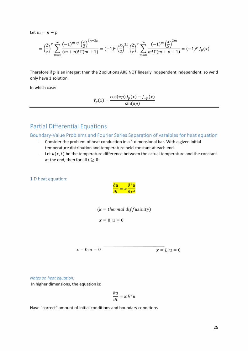
Therefore if 𝑝 is an integer: then the 2 solutions ARE NOT linearly independent independent, so we’d
only have 1 solution.
In which case:
𝑌𝑝(𝑥) =cos(𝜋𝑝) 𝐽𝑝(𝑥) − 𝐽−𝑝(𝑥)
sin(𝜋𝑝)
Partial Differential Equations
Boundary-Value Problems and Fourier Series Separation of varaibles for heat equation - Consider the problem of heat conduction in a 1 dimensional bar. With a given initial
temperature distribution and temperature held constant at each end.
- Let 𝑢(𝑥, 𝑡) be the temperature difference between the actual temperature and the constant
at the end, then for all 𝑡 ≥ 0:
1 D heat equation: 𝜕𝑢
𝜕𝑡= 𝜅
𝜕2𝑢
𝜕𝑥2
(𝜅 = 𝑡ℎ𝑒𝑟𝑚𝑎𝑙 𝑑𝑖𝑓𝑓𝑢𝑠𝑖𝑣𝑖𝑡𝑦)
Notes on heat equation:
In higher dimensions, the equation is:
𝜕𝑢
𝜕𝑡= 𝜅 ∇2𝑢
Have “correct” amount of Initial conditions and boundary conditions
𝑥 = 0; 𝑢 = 0
𝑥 = 0; 𝑢 = 0 𝑥 = 𝐿; 𝑢 = 0

26
Solving 1D heat equation: Separation of variables Separations of variables usually requires linear and homogeneous PDE with linear and homogeneous
Boundary conditions
Using separation of variables:
Let
𝑢 = 𝑋(𝑥)𝑇(𝑡)
∴𝜕𝑢
𝜕𝑡= 𝜅
𝜕2𝑢
𝜕𝑥2
⟹ 𝑋𝑇′ = 𝜅𝑋𝑇′′
∴𝑇′
𝜅𝑇=
𝑋′′
𝑋= 𝑘
(𝑠𝑜𝑚𝑒 𝑐𝑜𝑛𝑠𝑡𝑎𝑛𝑡, 𝑎𝑠 𝑡ℎ𝑒 𝑜𝑛𝑙𝑦 𝑤𝑎𝑦 𝑎 𝑓𝑢𝑛𝑐𝑡𝑖𝑜𝑛 𝑖𝑛 𝑡 𝑐𝑎𝑛 𝑒𝑞𝑢𝑎𝑙 𝑎 𝑓𝑢𝑛𝑐𝑡𝑖𝑜𝑛 𝑖𝑛 𝑥 𝑖𝑠 𝑖𝑓 𝑡ℎ𝑒𝑦 𝑎𝑟𝑒 𝑐𝑜𝑛𝑠𝑡𝑎𝑛𝑡)
𝑘 𝑐𝑎𝑛 𝑏𝑒 𝑒𝑖𝑡ℎ𝑒𝑟 + ,0 𝑜𝑟 −
Positive k: (trivial soluiton)
If 𝑘 is positive
𝑘 = 𝜆2 (𝜆 > 0)
∴ 𝑋′′ = 𝜆2𝑋
𝑋 = 𝐴𝑒𝜆𝑥 + 𝐵𝑒−𝜆𝑥
Boundary conditions:
𝑢 = 0, 𝑎𝑡 𝑥 = 0, 𝐿
𝑥 = 0: 𝑢(0, 𝑡) = 𝑋(0)𝑇(𝑡) = 0 → 𝑋(0) = 0
𝑥 = 𝑙: 𝑢(𝐿, 𝑡) = 𝑋(𝐿)𝑇(𝑡) = 0 → 𝑋(𝐿) = 0
∴ 𝑋(0) = 0; → 𝐴 + 𝐵 = 0;
𝑋(𝐿) = 0: 𝐴𝑒𝜆𝐿 − 𝐴𝑒−𝜆𝐿 = 0
∴ 𝐴 = 𝐵 = 0
Trivial solution.
∴ boring 0 solution
𝑘 = 0 trivial Solution:
𝑋′′ = 0
→ 𝑋 = 𝐴𝑥 + 𝐵
𝑋(0) = 0 → 𝐵 = 0
𝑋(𝐿) = 0 → 𝐴 = 0

27
𝑘 < 0 Solution:
𝑘 = −𝜆2 (𝑓𝑜𝑟 𝑠𝑜𝑚𝑒𝜆 > 0)
∴ 𝑋′′ + 𝜆2𝑋 = 0 𝑋 = 𝐴 cos(𝜆𝑥) + 𝐵 sin(𝜆𝑥)
𝑋(0) = 0 → 𝐴 = 0
𝑋(𝐿) = 0 → 𝐵 = 0 𝑜𝑟 sin(𝜆𝐿) = 0
∴ 𝜆 =𝑛𝜋
𝐿 (𝑓𝑜𝑟 𝑛 = 1,2,3 … ) (𝑜𝑛𝑙𝑦 𝑡𝑎𝑘𝑒 𝑛 ∈ ℤ+ 𝑎𝑠 𝜆, 𝐿 > 0)
∴⟹𝑇′
𝜅𝑇= 𝑘 = −𝜆2 = −
𝑛2𝜋2
𝐿2
∴ 𝑇′ = −𝑛2𝜋2
𝐿2 𝜅𝑇
(i.e. exponential decay)
∴ 𝑇 = 𝐶𝑛 𝑒−
𝑛2𝜋2
𝐿2 𝜅𝑡
(𝐶𝑛 as constant term will be detirmed by your 𝑛 eigenvalue values)
𝑢 = 𝑋𝑇 = 𝐴𝑛 sin (𝑛𝜋
𝐿𝑥) 𝑒
−𝑛2𝜋2
𝐿2 𝜅𝑡 (𝑓𝑜𝑟 𝑎𝑛𝑦 𝑝𝑜𝑠𝑖𝑡𝑖𝑣𝑒 𝑖𝑛𝑡𝑒𝑔𝑒𝑟 𝑛)
The heat equation is linear, and so by the method of superposition, the most general solution, where
all positible terms as a linaer combination is:
𝑢(𝑥, 𝑡) = ∑ 𝐴𝑛 sin (𝑛𝜋
𝐿𝑥) 𝑒
−𝑛2𝜋2
𝐿2 𝜅𝑡
∞
𝑛=1
The Initial conditions: 𝑢(𝑥, 0) = 𝑓(𝑥)
⟹ ∑ 𝐴𝑛 sin (𝑛𝜋
𝐿𝑥)
∞
𝑛=1
= 𝑓(𝑥)