Coupled spring equations

This article was downloaded by: [Nipissing University]On: 05 October 2014, At: 19:19Publisher: Taylor & FrancisInforma Ltd Registered in England and Wales Registered Number: 1072954Registered office: Mortimer House, 37-41 Mortimer Street, London W1T 3JH, UK

International Journal ofMathematical Education in Scienceand TechnologyPublication details, including instructions for authors andsubscription information:http://www.tandfonline.com/loi/tmes20

Coupled spring equationsTemple H. Fay a & Sarah Duncan Graham ba Technikon Pretoria and Mathematics, University of SouthernMississippi, Box 5045, Hattiesburg, MS 39406-5045, USA E-mail: [email protected] University of Southern MississippiPublished online: 11 Nov 2010.

To cite this article: Temple H. Fay & Sarah Duncan Graham (2003) Coupled spring equations,International Journal of Mathematical Education in Science and Technology, 34:1, 65-79, DOI:10.1080/0020739021000029258

To link to this article: http://dx.doi.org/10.1080/0020739021000029258

PLEASE SCROLL DOWN FOR ARTICLE

Taylor & Francis makes every effort to ensure the accuracy of all the information(the “Content”) contained in the publications on our platform. However, Taylor& Francis, our agents, and our licensors make no representations or warrantieswhatsoever as to the accuracy, completeness, or suitability for any purpose of theContent. Any opinions and views expressed in this publication are the opinions andviews of the authors, and are not the views of or endorsed by Taylor & Francis. Theaccuracy of the Content should not be relied upon and should be independentlyverified with primary sources of information. Taylor and Francis shall not be liablefor any losses, actions, claims, proceedings, demands, costs, expenses, damages,and other liabilities whatsoever or howsoever caused arising directly or indirectly inconnection with, in relation to or arising out of the use of the Content.

This article may be used for research, teaching, and private study purposes. Anysubstantial or systematic reproduction, redistribution, reselling, loan, sub-licensing,systematic supply, or distribution in any form to anyone is expressly forbidden.Terms & Conditions of access and use can be found at http://www.tandfonline.com/page/terms-and-conditions

http://www.tandfonline.com/loi/tmes20

http://www.tandfonline.com/action/showCitFormats?doi=10.1080/0020739021000029258

http://dx.doi.org/10.1080/0020739021000029258

http://www.tandfonline.com/page/terms-and-conditions

http://www.tandfonline.com/page/terms-and-conditions

Coupled spring equations

TEMPLE H. FAY*

Technikon Pretoria and Mathematics, University of Southern Mississippi, Box 5045,Hattiesburg, MS 39406-5045, USA

E-mail: [email protected]

and SARAH DUNCAN GRAHAM

University of Southern Mississippi

(Received 12 September 2002)

Coupled spring equations for modelling the motion of two springs withweights attached, hung in series from the ceiling are described. For the linearmodel using Hooke’s Law, the motion of each weight is described by a fourth-order linear differential equation. A nonlinear model is also described anddamping and external forcing are considered. The model has many features thatpermit the meaningful introduction of many concepts including: accuracy ofnumerical algorithms, dependence on parameters and initial conditions, phaseand synchronization, periodicity, beats, linear and nonlinear resonance, limitcycles, harmonic and subharmonic solutions. These solutions produce a widevariety of interesting motions and the model is suitable for study as a computerlaboratory project in a beginning course on differential equations or as anindividual or a small-group undergraduate research project.

1. IntroductionThe classical syllabus for beginning differential equations is rapidly changing

from emphasizing solution techniques for a variety of types of differentialequations to emphasizing systems and more qualitative aspects of the theory ofordinary differential equations. In particular, there is an emphasis on nonlinearequations due largely to the wide availability of high powered numerical algor-ithms and almost effortless graphics capabilities that come with computer algebrasystems such as Mathematica and Maple.

In this article, we investigate an old problem that appears now to be relegatedto the exercises in texts, if it appears at all (see for example [1, pp. 220–221]). Thisis the problem of two springs and two weights attached in series, hanging from theceiling. Under the assumption that the restoring forces behave according toHooke’s Law, this two degrees of freedom problem is modelled by a pair ofcoupled, second-order, linear differential equations. By differentiating and sub-stituting one equation into the other, the motion of each weight can be shown to bedetermined by a linear, fourth-order differential equation. We like this example forthis very reason, most models in elementary texts are only of second order.Moreover, the questions about phase now have a very nice physical interpretation;

int. j. math. educ. sci. technol., 2003vol. 34, no. 1, 65–79

International Journal of Mathematical Education in Science and TechnologyISSN 0020–739X print/ISSN 1464–5211 online # 2003 Taylor & Francis Ltd

http://www.tandf.co.uk/journalsDOI: 10.1080/0020739021000029258

*The author to whom correspondence should be addressed.

Dow

nloa

ded

by [

Nip

issi

ng U

nive

rsity

] at

19:

19 0

5 O

ctob

er 2

014

we can investigate when the motions of the two weights are synchronized (inphase) or opposing each other (1808 out of phase). By tinkering with the springconstants, oscillatory motions can be produced that are much more interestingthan those obtained from the classical single spring model. Moreover, there areother phenomena that can be investigated.

We also demonstrate, through examples, that interesting motions can arisewhen a slight nonlinearity is introduced in an attempt to make the restoring forcemore physically meaningful. In this situation, periodicity of the solutions becomesa more delicate matter. If forcing is introduced, subharmonic solutions of longperiods can be found which again exhibit more interesting motions than for theclassical linear case.

There is the opportunity here for many numerical and graphical investigationsto be made by students. Periodicity, amplitude, phase, sensitivity to inital con-ditions, and many more concepts can be investigated by modifying the parametersin the model. And of course, it would not be difficult for students to derive a modelfor three springs and three weights (or more), and to investigate the variousmotions that could arise from both linear and nonlinear restoring forces.

2. The coupled spring modelThe model consists of two springs and two weights. One spring, having spring

constant k1, is attached to the ceiling and a weight of mass m1 is attached to thelower end of this spring. To this weight, a second spring is attached having springconstant k2. To the bottom of this second spring, a weight of mass m2 is attachedand the entire system appears as illustrated in figure 1.

Allowing the system to come to rest in equilibrium, we measure the displace-ment of the centre of mass of each weight from equilibrium, as a function of time,and denote these measurements by x1ðtÞ and x2ðtÞ respectively.

2.1. Assuming Hooke’s LawUnder the assumption of small oscillations, the restoring forces are of the

form �k1l1 and �k2l2 where l1 and l2 are the elongations (or compressions) of

66 T. H. Fay and S. D. Graham

Figure 1. The coupled springs.

Dow

nloa

ded

by [

Nip

issi

ng U

nive

rsity

] at

19:

19 0

5 O

ctob

er 2

014

the two springs. Since the upper mass is attached to both springs, there aretwo restoring forces acting upon it: an upward restoring force �k1x1 exerted bythe elongation (or compression) x1 of the first spring; an upward force �k2ðx2 � x1Þfrom the second spring’s resistance to being elongated (or compressed) bythe amount x2 � x1. The second mass only ‘feels’ the restoring force fromthe elongation (or compression) of the second spring. If we assume there are nodamping forces present, then Newton’s Law implies that the two equationsrepresenting the motions of the two weights are

m1€xx1 ¼ �k1x1 � k2ðx1 � x2Þ

m2€xx2 ¼ �k2ðx2 � x1Þð2:1Þ

Thus we have a pair of coupled second-order linear differential equations.In order to find an equation for x1 that doesn’t involve x2, we solve the first

equation for x2, obtaining

x2 ¼m1€xx1k2

þ k1 þ k2k2

x1 ð2:2Þ

Substituting for x2 in the second differential equation (2.1), and simplifying, weobtain

m1m2xð4Þ1 þ ðm2k1 þ k2ðm1 þ m2ÞÞ€xx1 þ k1k2x1 ¼ 0 ð2:3Þ

Hence the motion of the first weight is determined by this fourth-order lineardifferential equation.

Now to find an equation that only involves x2, we solve the second equation(2.1) for x1:

x1 ¼m2

k2€xx2 þ x2 ð2:4Þ

and substitute into the first equation (2.1), producing the equation

m1m2xð4Þ2 þ ðm2k1 þ k2ðm1 þ m2ÞÞ€xx2 þ k1k2x2 ¼ 0 ð2:5Þ

This is exactly the same fourth-order equation as that for the motion of the firstweight. Thus the motions of each weight obey the same differential equation, andit is only the initial displacements and initial velocities that are needed in order tocompletely determine any specific case.

Typically, in a model of this sort, we would be given the initial displacementsx1ð0Þ and x2ð0Þ, and the initial velocities _xx1ð0Þ and _xx2ð0Þ. But in order to solveequations (2.3) and (2.5), we need to know the values of €xx1ð0Þ, xEEE1ð0Þ, €xx2ð0Þ andxEEE2ð0Þ. The values of the second derivatives are determined by evaluating equations(2.2) and (2.4) at time t ¼ 0. The values of the third derivatives are obtained byevaluating the derivatives of equations (2.2) and (2.4) at time t ¼ 0. Thus themotions for any set of initial conditions are determined by solving two fourth-order initial value problems.

Alternatively, we can turn this pair of coupled second-order equations into asystem of four first-order equations by setting _xx1 ¼ u and _xx2 ¼ v, so we have

Coupled spring equations 67

Dow

nloa

ded

by [

Nip

issi

ng U

nive

rsity

] at

19:

19 0

5 O

ctob

er 2

014

_xx1 ¼ u

_uu ¼ � k1m1

x1 �k2m1

ðx1 � x2Þ

_xx2 ¼ v

_vv ¼ � k2m2

ðx2 � x1Þ

ð2:6Þ

and we need only consider the four initial conditions x1ð0Þ, uð0Þ, x2ð0Þ, and vð0Þ.

2.2. Some examples with identical weightsLet us consider the model having the two weights of the same mass. This

model may be normalized by setting m1 ¼ m2 ¼ 1. In the case of no damping andno external forcing, the characteristic equation of the differential equations (2.3)and (2.5) is

m4 þ ðk1 þ 2k2Þm2 þ k1k2 ¼ 0 ð2:7Þ

which has the roots

�ffiffiffiffiffiffiffiffiffiffiffiffiffiffiffiffiffiffiffiffiffiffiffiffiffiffiffiffiffiffiffiffiffiffiffiffiffiffiffiffiffiffiffiffiffiffiffiffiffiffi�12k1 � k2 � 1

2

ffiffiffiffiffiffiffiffiffiffiffiffiffiffiffiffiffiffik21 þ 4k22

qrð2:8Þ

Example 2.1. Describe the motion for spring constants k1 ¼ 6 and k2 ¼ 4 withinitial conditions ðx1ð0Þ; _xx1ð0Þ, x2ð0Þ, _xx2ð0ÞÞ ¼ ð1; 0; 2; 0Þ.

It is easy to see that the roots of the characteristic equation are �ffiffiffi2

pi and

�2ffiffiffi3

pi. Thus the general solution to equations (2.3) and (2.5) is

xðtÞ ¼ c1 cosffiffiffi2

ptþ c2 sin

ffiffiffi2

ptþ c3 cos 2

ffiffiffi3

ptþ c4 sin 2

ffiffiffi3

pt ð2:9Þ

It is also easy to compute that ðx1ð0Þ; _xx1ð0Þ; €xx1ð0Þ; xEEE1ð0ÞÞ ¼ ð1; 0;�2; 0Þ. This leadsto the two pairs of simultaneous equations

c1 þ c3 ¼ 1ffiffiffi2

pc2 þ 2

ffiffiffi3

pc4 ¼ 0

�2c1 � 12c3 ¼ �2 � 2ffiffiffi2

pc2 � 24

ffiffiffi3

pc4 ¼ 0

ð2:10Þ

whose solutions are c1 ¼ 1, c3 ¼ 0, and c2 ¼ c4 ¼ 0. Thus the unique solution forx1ðtÞ is

x1ðtÞ ¼ cosffiffiffi2

pt ð2:11Þ

It is also easy to compute that ðx2ð0Þ; _xx2ð0Þ; €xx2ð0Þ; xEEE2ð0ÞÞ ¼ ð2; 0;�2; 0Þ. This leadsto the two pairs of simultaneous equations

c1 þ c3 ¼ 2ffiffiffi2

pc2 þ 2

ffiffiffi3

pc4 ¼ 0

�2c1 � 12c3 ¼ �4 � 2ffiffiffi2

pc2 � 24

ffiffiffi3

pc4 ¼ 0

ð2:12Þ

whose solutions are c1 ¼ 2, c3 ¼ 0, and c2 ¼ c4 ¼ 0. The unique solution for x2ðtÞ is

x2ðtÞ ¼ 2 cosffiffiffi2

pt ð2:13Þ


Dow

nloa

ded

by [

Nip

issi

ng U

nive

rsity

] at

19:

19 0

5 O

ctob

er 2

014

The motion here is synchronized and thus the weights move in phase with eachother, having the same period of motion, merely having different amplitudes; thisis shown in figure 2.1. Since the motion is simple periodic motion, the phaseportraits for x1 and x2 are simple closed curves (ellipses) as shown in the left-handframe in figure 2.2. Shown in the right-hand frame of figure 2.2 is a plot of x1against x2; observe this plot is a straight line of slope 2.

The next example illustrates 1808 out of phase motion.

Example 2.2. Describe the motion for spring constants k1 ¼ 6 and k2 ¼ 4 withinitial conditions ðx1ð0Þ; _xx1ð0Þ; x2ð0Þ; _xx2ð0ÞÞ ¼ ð�2; 0; 1; 0Þ.

In this example, for x1, we have c1 ¼ 0, c3 ¼ �2, and c2 ¼ c4 ¼ 0, and accord-ingly


Figure 2.1. Plot of x1 and x2 showing synchronized motion.

Figure 2.2. Plots for Example 2.1.

Dow

nloa

ded

by [

Nip

issi

ng U

nive

rsity

] at

19:

19 0

5 O

ctob

er 2

014

x1ðtÞ ¼ �2 cos 2ffiffiffi3

pt ð2:14Þ

For x2, we have c1 ¼ 0, c3 ¼ 1, and c2 ¼ c4 ¼ 0; thus

x2ðtÞ ¼ cos 2ffiffiffi3

pt ð2:15Þ

While the first weight is moving downward, the second weight is moving upwardand when the first is moving upward, the second is moving downward. Again bothmotions have the same period, the motions are 1808 out of phase. This is shown inthe left-hand frame of figure 2.3. In the right-hand frame we plot x1 against x2 andobserve a straight line of slope �1.

Generally speaking, the motions of the two weights will not be periodic, sincethe solutions for x1 and x2 are linear combinations of sin

ffiffiffi2

pt, cos

ffiffiffi2

pt, sin 2

ffiffiffi3

pt,

and cos 2ffiffiffi3

pt and the ratio of the frequencies

ffiffiffi2

pand 2

ffiffiffi3

pis not rational. For more

on the period of such combinations we refer the reader to [2].By tinkering with the parameters in this model, more interesting motions than

those just described can be obtained.

Example 2.3. Describe the motion for spring constants k1 ¼ 0:4 andk2 ¼ 1:808 with initial conditions ðx1ð0Þ; _xx1ð0Þ; x2ð0Þ; _xx2ð0ÞÞ ¼ ð1=2; 0;�1=2; 7=10Þ.

From equation (2.8), we see that it is the k1 and k2 values that completelydetermine the period and hence frequency of the response of this symmetricweight problem. Essentially the initial conditions only affect the amplitude andphase of the solutions. Thus, using a numerical solver and ‘tweaking’ the k valuesand experimenting with the initial conditions led to the choice of parameters in thisexample. This type of numerical and graphical interactive investigation can becarried out with a computer algebra system almost effortlessly. The phase portraitsfor the two solutions are shown in the top row of figure 2.4. These portraits showan interesting (almost?) period motion. Plots of the actual solutions are shown inthe middle row. Plotting both solutions together on the same coordinate systemalso shows an interesting pattern. This is shown in the left-hand frame of thebottom row of figure 2.4. Finally, the plot of x1 against x2 shown in the right-handframe of the bottom row of figure 2.4 appears to be a Lissajous type curve.

Student problem. Verify analytically the solutions to this initial value problemare periodic. Find the period. Use the analytic solution to produce other periodicmotions.



Dow

nloa

ded

by [

Nip

issi

ng U

nive

rsity

] at

19:

19 0

5 O

ctob

er 2

014

2.3. Damping

The most common type of damping encountered in beginning courses is that of

viscous damping; the damping force is proportional to the velocity. The damping

of the first weight depends solely on its velocity and not the velocity of the second

weight, and vice versa. We add viscous damping to the model by adding the term



Dow

nloa

ded

by [

Nip

issi

ng U

nive

rsity

] at

19:

19 0

5 O

ctob

er 2

014

��1 _xx1 to the first equation and ��2 _xx2 to the second equation (2.1). We assume thatthe damping coefficients �1 and �2 are small. The model becomes

m1€xx1 ¼ ��1 _xx1 � k1x1 � k2ðx1 � x2Þ

m2€xx2 ¼ ��2 _xx2 � k2ðx2 � x1Þ ð2:16Þ

To obtain an equation for the motion x1 which does not involve x2, we solve thefirst equation (2.16) for x2 and substitute into the second equation (2.16) to obtain

m1m2xð4Þ1 þ ðm1�1 þm2�2ÞxEEE1 þ ðm2k1 þ k2ðm1 þ m2Þ þ �1�2Þ€xx1

þðk1�2 þ k2ð�1 þ �2Þ _xx1 þ k1k2x1 ¼ 0 ð2:17Þ

In a similar manner, we may solve the second equation (2.16) for x1 and substituteinto the first equation to obtain a fourth-order equation that involves only x2. Weobtain

m1m2xð4Þ2 þ ðm1�1 þ m2�2ÞxEEE2 þ ðm2k1 þ k2ðm1 þ m2Þ þ �1�2Þ€xx2

þðk1�2 þ k2ð�1 þ �2Þ _xx2 þ k1k2x2 ¼ 0 ð2:18Þ

So once again we have the same linear differential equation representing themotion of both weights.

The roots of the characteristic equation are now more complicated to discuss ingeneral, but not surprisingly, we obtain damped oscillatory motion for bothweights under simple assumptions on the parameters.

Example 2.4. Assume m1 ¼ m2 ¼ 1. Describe the motion for spring constantsk1 ¼ 0:4 and k2 ¼ 1:808, damping coefficients �1 ¼ 0:1 and �2 ¼ 0:2, with initialconditions ðx1ð0Þ; _xx1ð0Þ; x2ð0Þ; _xx2ð0ÞÞ ¼ ð1; 1=2; 2; 1=2Þ.

The phase portraits for x1 and x2 are shown in the top row of figure 2.5; onesees a regular pattern of motion with diminishing amplitude. Damped oscillatorymotion is evident in plots of the solutions shown in the middle row; and in the left-hand frame of the bottom row, we plot both x1 and x2 and observe nearlysynchronized motion. Finally, in the right-hand frame of the bottom row, weplot x1 versus x2 which also shows damped oscillatory motion of both weights.

Student problem. Investigate the model when �1 ¼ 0 and �2 > 0. What hap-pens if �1 > 0 and �2 ¼ 0?

Student problem. What are the conditions on the parameters of the model thatgive rise to critically damped motion and over-critically damped motion, or dothese concepts not apply to this model?

3. Adding nonlinearityIf we assume that the restoring forces are nonlinear, which they most certainly

are for large vibrations, we can modify the model accordingly. Rather thanassuming that the restoring force is of the form �kx (Hooke’s law), suppose weassume the restoring force has the form �kxþ �x3. Then our model becomes


Dow

nloa

ded

by [

Nip

issi

ng U

nive

rsity

] at

19:

19 0

5 O

ctob

er 2

014

m1€xx1 ¼ ��1 _xx1 � k1x1 þ �1x31 � k2ðx1 � x2Þ þ �2ðx1 � x2Þ3

m2€xx2 ¼ ��2 _xx2 � k2ðx2 � x1Þ þ �2ðx2 � x1Þ3 ð3:1Þ

The range of motions for the nonlinear model is much more complicated than thatfor the linear model. To get an idea of this range of motions for a single spring



Dow

nloa

ded

by [

Nip

issi

ng U

nive

rsity

] at

19:

19 0

5 O

ctob

er 2

014

model see [4]. Moreover, accuracy questions arise when solving these equations.No numerical solver can be expected to remain accurate over long time intervals.The accumulated local truncation error, algorithm error, roundoff error, propaga-tion error, etc., eventually force the numerical solution to be inaccurate. This isdiscussed in some detail in the interesting paper by Knapp and Wagon [7], see also[3] and [5].

Example 3.1. Assume m1 ¼ m2 ¼ 1. Describe the motion for spring constantsk1 ¼ 0:4 and k2 ¼ 1:808, damping coefficients �1 ¼ 0 and �2 ¼ 0, nonlinearcoefficients �1 ¼ �1=6 and �2 ¼ �1=10, with initial conditionsðx1ð0ÞÞ; _xx1ð0Þ; x2ð0Þ; _xx2ð0ÞÞ ¼ ð1; 0;�1=2; 0Þ.

The motion in this example is quite nice. We have no damping, so the motionsare oscillatory and appear to be periodic (for more on detecting and describingperiodic solutions to nonlinear differential equations see [6]). Phase plane trajec-tories are shown in the top row of figure 3.1 for 04 t4 50; solutions are shown inthe middle row. A plot of x1 and x2 shows the motions that appear to be 1808 out ofphase, see the left-hand frame of the bottom row. A plot of x1 against x2 is given inthe right-hand frame.

Because of the nonlinearity, the model may exhibit sensitivity to initialconditions.

Example 3.2. Assume m1 ¼ m2 ¼ 1. Describe the motion for spring constantsk1 ¼ 0:4 and k2 ¼ 1:808, damping coefficients �1 ¼ 0 and �2 ¼ 0, nonlinear coeffi-cients �1 ¼ �1=6 and �2 ¼ �1=10, with initial conditions ðx1ð0Þ; _xx1ð0Þ; x2ð0Þ;_xx2ð0ÞÞ ¼ ð�0:5; 1=2; 3:001; 5:9Þ.

Phase plots and a plot of x1 versus x2 are shown in figures 3.2 and 3.3. Verypleasing motions can be observed here. Next we change only the x1ð0Þ value by 1/10, and we obtain quite different motions.

Example 3.3. Assume m1 ¼ m2 ¼ 1. Describe the motion for spring constantsk1 ¼ 0:4 and k2 ¼ 1:808, damping coefficients �1 ¼ 0 and �2 ¼ 0, nonlinear coeffi-cients �1 ¼ �1=6 and �2 ¼ �1=10, with initial conditions ðx1ð0Þ; _xx1ð0Þ; x2ð0Þ;_xx2ð0ÞÞ ¼ ð�0:6; 1=2; 3:001; 5:9Þ.

The phase plots for this example are shown in figure 3.4 for 04 t4 200. A plotof x1 versus x2 is shown in figure 3.5.

4. Adding forcingIt is a simple matter to add external forcing to the model. Indeed, we can drive

each weight differently. Suppose we assume simple sinusoidal forcing of the formF cos!t. Then the model becomes

m1€xx1 ¼ ��1 _xx1 � k1x1 þ �1x31 � k2ðx1 � x2Þ þ �2ðx1 � x2Þ3 þ F1 cos!1t

m2€xx2 ¼ ��2 _xx2 � k2ðx2 � x1Þ þ �2ðx2 � x1Þ3 þ F2 cos!2t ð4:1Þ

The range of motions for nonlinear forced models is quite vast. We can expect tofind bounded and unbounded solutions (nonlinear resonance), periodic solutionsthat share the period with the forcing (called harmonic solutions) and solutionsthat are periodic of period a multiple of the driving period (called subharmonic


Dow

nloa

ded

by [

Nip

issi

ng U

nive

rsity

] at

19:

19 0

5 O

ctob

er 2

014

solutions), and steady state periodic solutions (limit cycles in the phase plane). Theconditions under which these motions occur are by no means easy to state. Weconclude with a simple forced example.

Example 4.1. Assume m1 ¼ m2 ¼ 1. Describe the motion for spring constantsk1 ¼ 2=5 and k2 ¼ 1, damping coefficients �1 ¼ 1=10 and �2 ¼ 1=5, nonlinear



Dow

nloa

ded

by [

Nip

issi

ng U

nive

rsity

] at

19:

19 0

5 O

ctob

er 2

014


Figure 3.2. Phase plots for Example 3.2.

Figure 3.3. x1 versus x2, 04 t4 200, for Example 3.2.

Dow

nloa

ded

by [

Nip

issi

ng U

nive

rsity

] at

19:

19 0

5 O

ctob

er 2

014


Figure 3.4. Phase plots for Example 3.3.

Figure 3.5. x1 versus x2, 04 t4 200, for Example 3.3.

Dow

nloa

ded

by [

Nip

issi

ng U

nive

rsity

] at

19:

19 0

5 O

ctob

er 2

014

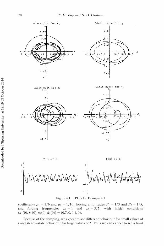
coefficients �1 ¼ 1=6 and �2 ¼ 1=10, forcing amplitudes F1 ¼ 1=3 and F2 ¼ 1=5,and forcing frequencies !1 ¼ 1 and !2 ¼ 3=5, with initial conditionsðx1ð0Þ; _xx1ð0Þ; x2ð0Þ; _xx2ð0ÞÞ ¼ ð0:7; 0; 0:1; 0Þ.

Because of the damping, we expect to see different behaviour for small values oft and steady-state behaviour for large values of t. Thus we can expect to see a limit


Figure 4.1. Plots for Example 4.1

Dow

nloa

ded

by [

Nip

issi

ng U

nive

rsity

] at

19:

19 0

5 O

ctob

er 2

014

cycle in the phase plane for both x1 and for x2. The trajectories and limit cycles areshown in the top and middle rows of figures 4.1. In the bottom row we show plotsof x1 and x2 for 04 t4 150. In the left-hand frame of figure 4.2, we plot both x1and x2 for 1104 t4 170 to show the steady-state solutions more clearly. We plotx1 against x2 in the steady state in the right-hand frame.

5. ConclusionsWe have developed a simple model for two coupled springs, examined both the

linear case and one possible form for the nonlinear case, and have included freemotion, damped motion, and forced motion examples. These examples producedinteresting solutions and are no more difficult for a student to produce than theelementary examples commonly encountered in beginning courses. This modelreinforces much of the theory for linear equations and provides a nice elementarymodelling example that can be used in a computer laboratory component of abeginning course or for an individual or a small-group undergraduate researchproject.

The model has many features that permit the meaningful introduction of manyconcepts including: accuracy of numerical algorithms, dependence on parametersand initial conditions, phase and synchronization, periodicity, beats, limit cycles,harmonic and subharmonic solutions. The use of a computer algebra systempermits almost effortless numerical explorations, graphical interpretations, andmotivation for analytical verifications.

References[1] Boyce, W. E., and DiPrima, R. C., 2001, Elementary Differential Equations, 7th edition

(New York: John Wiley & Sons).[2] Fay, T. H., 2000, Int. J. Math. Educ. Sci. Technol., 31, 733–747.[3] Fay, T. H., and Joubert, S. V., 1999, Math. Comput. Educ., 33, 67–77.[4] Fay, T. H., and Joubert, S. V., 1999, Int. J. Math. Educ. Sci. Technol., 30, 889–902.[5] Fay, T. H., and Joubert, S. V., 2000, Math. Mag., 73, 393–396.[6] Fay, T. H., and Joubert, S. V., 2000, Int. J. Math. Educ. Sci. Technol., 31, 825–838.[7] Knapp, R., and Wagon, S., C�ODE�E (winter 1996), pp. 9–13.


Figure 4.2. Plot of x1 and x2 for Example 4.1.

Dow

nloa

ded

by [

Nip

issi

ng U

nive

rsity

] at

19:

19 0

5 O

ctob

er 2

014

Documents

Coupled spring equations