Incomplete quenching in a system of heat equations

coupled at the boundary

Raul Ferreira

Departamento de Matematicas, U. Complutense de Madrid, 28040 Madrid, Spain.

e-mail: raul−ferreira@ucm.es

Arturo de Pablo

Departamento de Matematicas, U. Carlos III de Madrid, 28911 Leganes, Spain.

e-mail: arturop@math.uc3m.es

Mayte Perez-LLanos

Departamento de Matematicas, U. Carlos III de Madrid, 28911 Leganes, Spain.

e-mail: mtperez@math.uc3m.es

Julio D. Rossi

Departamento de Matematica, FCEyN UBA, 1428 Buenos Aires, Argentine.

e-mail: jrossi@dm.uba.ar

Abstract

In this paper we find a possible continuation for quenching solutions to a system of heat equa-

tions coupled at the boundary condition. This system exhibits simultaneous and non-simultaneous

quenching. For non-simultaneous quenching our continuation is a solution of a parabolic prob-

lem with Neumann boundary conditions. We also give some results for simultaneous quenching

and present some numerical experiments that suggest that the approximations are not uniformly

bounded in this case.

2000 AMS Subject Classification: 35B40, 35B60, 35K50.

Keywords and phrases: quenching, non-simultaneous, incomplete.

1 Introduction and main results

Our main concern in this paper is to look for a possible continuation after quenching of solutionsto a system of heat equations coupled at the boundary.

We consider the following parabolic system: two heat equations,{ut = uxx

vt = vxx0 < x < 1 , 0 < t < T, (1.1)

coupled through a non linear flux at x = 0,{ux(0, t) = v−p(0, t)vx(0, t) = u−q(0, t)

0 < t < T, (1.2)

1

and zero flux at x = 1, {ux(1, t) = 0vx(1, t) = 0

0 < t < T. (1.3)

As initial condition we take

{u(x, 0) = u0(x)v(x, 0) = v0(x)

0 < x < 1. (1.4)

being u0, v0 positive, smooth and satisfying the compatibility conditions with the boundarydata. We also assume that u′0, v

′0 ≥ 0 and u′′0, v

′′0 < 0. By classical theory, local existence for the

solutions up to some time t = T (maximal existence time) is easily deduced. Moreover, solutionsare decreasing in time and increasing in space.

In [FPQR] the authors study this problem and find that, due to the absorption generatedby the boundary condition at x = 0, the solutions decrease to zero at this point. If they vanishin finite time t = T0, the boundary condition (1.2) blows up and the solution, being classical upto t = T , no longer exists (as a classical solution) for greater times, thus the maximal existencetime of a classical solution is T = T0.

This phenomenon of existence of a finite time t = T at which some term of the problem ceasesto make sense is known as quenching (T denotes the quenching time). It was studied for the firsttime in [K]. Since then, the phenomenon of quenching for different problems has been the issueof intensive study in recent years, see for example, [C, CK, DX, FPQR, FL, KN, L, L2, L3, PQR],and the references therein.

Some questions related to this situation naturally arise. For instance: how rapidly thesolutions tend to zero, the quenching rate, see [CK, L]; the extinction set for the solutions andtheir behavior near these points, the quenching set and the quenching profile, see [L, L2]; thepossibility of extending the solution in some weak sense after quenching, see [FG].

Dealing with a system of equations it is also interesting to guess whether the componentsof the solution quench (reach zero) at the same time (simultaneous quenching) or if some com-ponent quenches at time T while the other components remain bounded away from zero (non-simultaneous quenching), [FPQR, PQR]. In the case of non-simultaneous quenching, the fluxat the boundary of the quenching variable remains bounded. Nevertheless, its time derivativeblows up. In fact, both time derivatives blow up, see [FPQR]. Hence quenching is always si-multaneous in the sense of [K]. Simultaneous vs. non-simultaneous phenomenon has been alsoanalyzed in the case of blow-up, see for instance [PQR, QR1, QR2, ST].

We enclose in the following theorem the results obtained in [FPQR] concerning simultaneousvs. non-simultaneous quenching for our problem (1.1)–(1.4).

Theorem ([FPQR])i) If p, q ≥ 1 the quenching is always simultaneous, while if p < 1, we can find initial conditionsgiving rise to non-simultaneous quenching, i.e., such that u quenches and v remains boundedbelow (analogous result when q < 1).ii) If q < 1 and p ≥ p0 = (1+q)/(1−q) > 1, simultaneous quenching is not possible. Nevertheless,if 0 ≤ p, q ≤ 1 simultaneous quenching occurs for some initial conditions.

The restriction p ≥ p0 instead of p ≥ 1 in ii) seems to be technical. We will not require sucha condition in the present work.

2

Another important issue, as we have mentioned, is to see if it is possible in some sense tocontinue the solution (u, v) beyond t = T . This question was raised first for blow-up problems,see [BC, GV1, GV2, L, QRV], etc. In [FG] it was answered for a quenching problem for the heatequation with a nonlinear boundary condition. There the authors find that the continuation isa solution to the heat equation with a Dirichlet boundary condition, u(0, t) = 0, replacing thenonlinear flux at x = 0 and as initial condition at t = T the final profile of the original solution,u(x, T ).

The purpose of this work is to find, if possible, a natural continuation for problem (1.1)–(1.4)for times beyond T . To this end we approximate the involved powers by bounded functions andthen try to pass to the limit in the approximations. Let

fn(s) =

s−q, if s > 1/n,nq+1s, if 0 < s ≤ 1/n,0 if s < 0,

(1.5)

and

gn(s) =

s−p, if s > 1/n,np+1s, if 0 < s ≤ 1/n,0 if s < 0,

(1.6)

and let (un, vn) be the solution to problem (1.1) − (1.4) with fn and gn as boundary data, i.e.,

(un)x(0, t) = gn(vn(0, t)), (vn)x(0, t) = fn(un(0, t)).

Since fn and gn are bounded functions the solution (un, vn) is defined for all t > 0. A naturalattempt to obtain a continuation of (u, v) after quenching is to pass to the limit as n → ∞ in(un, vn).

Our first result assures that it is possible to take this limit and that it indeed gives acontinuation of (u, v) after T when blow-up is non-simultaneous. Moreover, we identify thePDE system verified by the continuation after quenching.

Theorem 1.1 Assume that u quenches while v remains bounded from below. Then the approx-imations (un, vn) have a finite limit

(u, v) = limn→∞

(un, vn), for all 0 ≤ x ≤ 1, t > 0, (1.7)

which is an extension of (u, v), that is, for every t < T it holds that (u, v) ≡ (u, v).Moreover, for every t > T , (u, v) is the solution to the system

ut = uxx,ux(0, t) = (v)−p(0, t),ux(1, t) = 0,u(x, T ) = u(x, T ),

vt = vxx, 0 < x < 1, t > T,vx(0, t) = 0, t > T,vx(1, t) = 0, t > T,v(x, T ) = v(x, T ), 0 ≤ x ≤ 1.

(1.8)

This result provides us with a natural continuation (u, v) of (u, v) after quenching. Notethat the v variable does not quench and continues as a solution of the heat equation withzero boundary flux, while the quenching variable u continues with boundary flux given by v−p.Therefore the system becomes partially decoupled.

3

For a single equation, see [FG], it happens that the continuation verifies a Dirichlet boundarycondition at x = 0. However, in Theorem 1.1 the boundary conditions verified by the contin-uation are of Neumann type. This says that a possible continuation for systems may stronglydiffer from a possible continuation for a single equation.

In the simultaneous quenching case the situation becomes more involved.As we have mentioned, when p = q and u0 = v0, the system reduces to a single equation, and

the continuation verifies a Dirichlet problem after T . We can show that this type of continuationis not generic.

In the general case, we can only prove that un, vn are bounded in compact intervals of timewhen p and q are less than one. However, passing to the limit in the system seems delicate,since we cannot find a priori estimates uniformly in n that ensure that the fluxes fn(un(0, t))and gn(vn(0, t)) converge to some limits.

The situation can be even worse for p or q greater than one. We conjecture in this case thatthe sequence (un, vn) is not bounded below near T (and therefore we cannot take the limit).Numerical experiments support this conjecture, see Section 4.

Remark 1.1 All the results in this article are also valid if we replace the flux at the boundary ofthe regularized problems, fn and gn, by smooth approximating functions, fn and gn, respectively,such that fn ≤ Cfn and gn ≤ Cgn, for some C > 0.

The rest of the paper is organized as follows: in Section 2 we prove Theorem 1.1 thatdeals with the non-simultaneous quenching case; in Section 3 we present some partial resultsconcerning the simultaneous case and finally in Section 4 we perform some numerical experimentsthat illustrate our results.

2 Non-simultaneous quenching.

Recall that we are considering the approximating problems (Pn) where we have replaced theinvolved powers by continuous and bounded functions, that is,

(Pn)

(un)t = (un)xx, ,(un)x(0, t) = gn(vn(0, t)),(un)x(1, t) = 0,un(x, 0) = u0(x),

(vn)t = (vn)xx, 0 < x < 1, t > 0,(vn)x(0, t) = fn(un(0, t)), t > 0,(vn)x(1, t) = 0, t > 0,vn(x, 0) = v0(x), 0 ≤ x ≤ 1,

where fn and gn are given by (1.5) and (1.6), respectively.

Solutions to this problem satisfy the following lemma.

Lemma 2.1 There exists a unique global in time solution to (Pn), such that

un, vn ∈ C2,1((0, 1) × [0, τ ]),

for every τ > 0, verifying:i) (un, vn) is uniformly bounded from above;ii) (un, vn) ≥ (u, v), for (x, t) ∈ [0, 1] × [0, T ).

4

Proof. To prove i) we only note that both functions are subsolutions of problem

wt = wxx, 0 < x < 1, t > 0,wx(0, t) = wx(1, t) = 0, t > 0,w(x, 0) = max(‖v0‖∞ , ‖u0‖∞), 0 ≤ x ≤ 1.

In order to prove ii), let us denote ψ = u−un and ω = v− vn, with (un, vn) solution to (Pn)with initial condition (u0 − ε, v0 − ε) for some ε > 0. So ψ(x, 0), ω(x, 0) < 0.

Let us suppose that there exists a first time t0 and some point x0 ∈ [0, 1] such that ψ(x0, t0) =0 and ω(x, t0) ≤ 0 (the opposite situation is similar). By the Strong Maximum Principlex0 ∈ {0, 1}. This cannot happen at x0 = 1, since ψx(1, t) = 0 and it contradicts Hopf’s Lemma.Thus, x0 = 0 and from Hopf’s Lemma it follows that ψx(0, t0) < 0.

But, on the other hand

ψx(0, t) = v−p(0, t) − gn(un(0, t)) ≥ v−p − (vn)−p ≥ −p|ξ|−p−1ω(0, t) ≥ 0

and we arrive to a contradiction. Finally, taking ε→ 0 we obtain de desired result. 2

The estimate proved in the last lemma allows us to consider the limit in (1.7), at least for0 < t < T . This limit coincides with the solution (u, v) for t < T as we show now.

Lemma 2.2 Let (u, v) be the function defined in (1.7). Then, for every t < T it holds that(u, v) ≡ (u, v).

Proof. For any fixed t0 < T there exists a constant c > 0 such that u(x, t), v(x, t) ≥ c, forevery 0 ≤ x ≤ 1 and t ≤ t0. If we take n0 verifying 1/n0 < c, then for every n ≥ n0 (u, v) solvesproblem (Pn) in (0, t0] × (0, 1) and by uniqueness of the solution we conclude (un, vn) = (u, v)in [0, t0] × [0, 1] for n ≥ n0. Therefore

(u, v) = limn→∞

(un, vn) = (u, v), (2.1)

for every t ∈ [0, t0] and every x ∈ [0, 1]. The arbitrariness of t0 gives that (2.1) holds for anyt < T . 2

Note that (un, vn) verifies (un)t, (vn)t ≤ 0 and (un)xx, (vn)xx ≤ 0 for times smaller than τn,the first time where one of the components reaches 1/n.

Let us suppose, from now on, that u quenches while v does not, i.e., v(0, t) ≥ c > 0 for all0 ≤ t ≤ T . Note that, by the results of [FPQR] this fact implies q < 1.

We want to show that the possible extension, (u, v), of the solution for t > T is the uniquepair of functions satisfying the system (1.8). To this end we prove that, for n large enough(un, vn) is a solution to the same system (1.8). We remark that, since v does not quench gn

remains being the power (vn)−q(0, t) for all t > 0 while the function fn in (Pn) turns to benp+1 un(0, t).

The next lemma will play a crucial role in our arguments. It says that for n large enough, inthe approximating problems the un variable reaches zero, while vn stays positive and boundedaway from zero uniformly in n.

Lemma 2.3 For each n sufficiently large, there exists a time Tn, such that un(0, t) ≤ 0, for allt ≥ Tn. Moreover, at that time c ≤ vn(0, Tn) ≤ C for some constants c, C > 0 independent of n.

5

Proof. Since the quenching is non-simultaneous there exists a time τn < T (with τn → T ) suchthat u(0, τn) = 1/n and v(0, τn) = cn ≥ c. Notice that we have (un, vn) = (u, v) for t ∈ (0, τn).Then, at time t = τn the functions un and vn are increasing and concave. Therefore,

c ≤ vn(x, τn) ≤ vn(0, τn) + nqx ≤ C + nqx ,

1

n≤ un(x, τn) ≤ 1

n+ (vn)−p(0, τn)x ≤ 1

n+Cx .

(2.2)

Now, we estimate the time τn at which vn reaches the level c/2 (if there is such a time).Denote by s(x, t) = vn(x, t + τn). Since s(x, 0) = v(x, τn) ≥ c and sx(0, t) = fn(un(0, t)) ≤ nq,we have that s is supersolution to the problem

ht = hxx, 0 < x < 1, 0 < t <∞,hx(0, t) = nq, 0 ≤ t <∞,hx(1, t) = 0, 0 ≤ t <∞,h(x, 0) = c, 0 ≤ x ≤ 1.

It is easy to see that the function h is decreasing in time and then, it is concave and increasing.Moreover, integrating the equation we have that

d

dt

∫ 1

0h(x, t) dx = −nq .

Therefore, h(0, t) vanishes in finite time. Let us denote by τ0 a time such that h(0, τ0) = c/2.We wish now to estimate τ0, that is, a lower bound for τn. Rescaling h as follows we take offthe dependence on n in the boundary condition. Let

ψ(y, τ) = h(y/nq, τ/n2q).

which satisfies the problem

ψτ = ψyy, 0 < y < nq, 0 < τ <∞,ψy(0, τ) = 1, 0 ≤ τ <∞,ψy(n

q, τ) = 0, 0 ≤ τ <∞,ψ(y, 0) = c, 0 ≤ y ≤ nq.

Then, there exists a time τ1 at which ψ(0, τ1) = c/2. We have also that ψ(0, τ1) = h(0, τ1/n2q),

thus,τn ≥ τ0 = τ1/n

2q.

We claim that, for n large enough, there exists a time τn ≤ τn such that u(0, τn) = 0.We observe that for t ∈ (0, τn) the function un verifies that (un)x(0, t) = v−p

n (0, t). Therefore,denoting r(x, t) = un(x, t+ τn), we have that r is subsolution to the linear problem

rt = rxx, 0 < x < 1, 0 < t < τn,rx(0, t) = C−p, 0 < t ≤ τnrx(1, t) = 0, 0 < t ≤ τn,r(x, 0) = u(x, τn), 0 ≤ x ≤ 1,

(2.3)

6

for a constant C > 0 such that vn(0, t) ≤ C. Integrating the equation in (2.3) we obtain that

d

dt

∫ 1

0r(x, t) dx = −C−p,

which implies that there exists a time τ0 such that r(0, τ0) = 0. Moreover r(0, t) < 0 from thistime on. In order to estimate τ0, which is an upper bound for τn, we rescale r as follows

ω(y, τ) = n r(y/n, τ/n2) .

The problem satisfied by ω is

ωτ = ωyy, 0 < y < n, 0 < τ <∞,ωy(0, τ) = C−p, 0 ≤ τ <∞,ωy(n, τ) = 0, 0 ≤ τ <∞,ω(y, 0) = n u(y/n, τn), 0 ≤ y ≤ n.

Using (2.2) to estimate the initial value ω(y, 0) = n u(y/n, τn) ≤ Cy + 1, it is easy to see thatthere exists a time τ1 (bounded independently of n), such that ω(0, τ 1) = 0.

Observe that 0 = ω(0, τ 1) = n r(0, τ 1/n2). Thus

τn ≤ τ0 = τ1/n2 ≤ C/n2.

Finally, from our bounds on τn and τn, using precisely that q < 1, for n large enough it holdsthat

τn ≤ τn.

This fact means that at the time Tn at which un vanishes, vn remains positive. Note thatfor times greater than Tn, vn is a solution to the heat equation with homogeneous Neumannboundary conditions. The proof is now complete. 2

To finish this section we have to prove that we can pass to the limit as in (1.7) and that(u, v) is indeed a solution to (1.8).

Proof.[End of the proof of Theorem 1.1] From the previous lemma we obtain that the sequencevn are uniformly bounded away zero uniformly in n. On the other hand, by Lemma 2.1 thesequence vn are uniformly bounded from above. Thus, we have that

C1 < vn(x, t) < C2.

Also from Lemma 2.1, we obtain that un(x, t) < C3. To obtain a lower bound, we note that,for n large, un is supersolution of

wt = wxx 0 < x < 1, t > 0,

wx(0, t) = C−p1 , t > 0,

wx(1, t) = 0, t > 0,w(x, 0) = u0(x).

Therefore, (un, vn) are uniformly bounded in compact sets. So, taking a subsequence ifnecessary, we have that there exists the limit (un, vn) → (u, v).

7

Our next aim is to identify the PDE system verified by this limit after T .Now we just observe that (un, vn) is a solution to

(un)t = (un)xx, ,(un)x(0, t) = (vn)−p(0, t),(un)x(1, t) = 0,

(vn)t = (vn)xx, 0 < x < 1, t > Tn,(vn)x(0, t) = 0, t > Tn,(vn)x(1, t) = 0, t > Tn,

(2.4)

where Tn is the first time at which un(x, Tn) = 0. From the estimates obtained in the previouslemma, we have that τn < Tn < τn + C/n2. Thus, it holds that

limn→∞

Tn = T.

First, we want to pass to the limit in the v-variable. To this end we write down the integralversion of the problem for vn,

−∫ t

Tn

∫ 1

0vnϕt +

∫ 1

0vn(t)ϕ(t) −

∫ 1

0vn(Tn)ϕ(Tn) =

∫ t

Tn

∫ 1

0vnϕxx −

∫ t

Tn

vnϕx

∣∣∣1

0. (2.5)

It is easy to see that we can pass to the limit in all the terms of the above identity, the onlytricky point is to show that

vn(x, Tn) → v(x, T ). (2.6)

In order to prove this we just consider the Green function of the Neumann problem, G. Therefore,for times τn ≤ t ≤ Tn we can write

vn(x, t) =

∫ 1

0G(x− y, t)v(y, τn) dy +

∫ t

τn

G(x, t− s)(vn)x(0, s) ds. (2.7)

We have that the first integral goes uniformly to v(x, T ) while the second one is bounded byCnq−1 (we are using here that Tn − τn ≤ Cn−2 and that (vn)x = fn(un) ≤ Cnq+1). Since q < 1this last term goes to zero. This completes the proof for the v-component.

For the u-component passing to the limit is even easier since vn are uniformly bounded belowaway from zero. Thus we can pass to the limit in the weak form of the problem (analogous to(2.5)) beginning at t = 0. 2

3 Simultaneous quenching

In this section we collect some results concerning the simultaneous case. Hence, let us supposethat u and v quench at the same time T .

Now we state a lemma that shows that, under certain conditions on the exponents and theinitial conditions, we can compare un and vn.

Lemma 3.1 i) Let q ≤ p and u0(x) < v0(x) with ‖v0‖∞ ≤ 1. Then un(x, t) ≤ vn(x, t)ii) Let q ≥ p and u0(x) > v0(x) with u0(0) ≤ 1. Then un(x, t) ≥ vn(x, t)

Proof. To prove i), let us denote ψ = un − vn. So ψ(x, 0) < 0. Assume that there exists a firsttime t0 and some point x0 ∈ [0, 1] such that ψ(x0, t0) = 0. By the Strong Maximum Principle

8

x0 ∈ {0, 1}. This cannot happen at x0 = 1, since ψx(1, t) = 0 and it contradicts Hopf’s Lemma.Thus x0 = 0 and from Hopf’s Lemma it follows that ψx(0, t0) < 0.

In order to get a contradiction we consider 3 different cases:1) If no truncation takes place, then ψx(0, t0) = v−p

n (0, t0)(1 − vp−qn (0, t0)) ≥ 0; in this case

vn(0, t0) ≤ 1 (since the initial data are both bounded by one).2) if only one truncation takes place, then un(0, t0) ≤ 1/n < vn(0, t0);3) if both truncations take place, then ψx(0, t0) = np+1vn(0, t0)(1 − nq−p) ≥ 0.Interchanging the roles of p and q, un and vn, we obtain the second statement. 2

We define for n fixed the sets

An = {(u0, v0) | ∃tn such that : un(0, tn), vn(0, tn) ≤ 0},Bn = {(u0, v0) | ∃tn such that : un(0, tn) ≤ 0, and vn(0, t) > 0, ∀t},Bn = {(u0, v0) | ∃tn such that : vn(0, tn) ≤ 0, and un(0, t) > 0, ∀t},Cn = {(u0, v0) | un(0, t) > 0, vn(0, t) > 0,∀t}.

(3.1)

Notice that from Lemma 3.1 we deduce that Bn ∪ Bn are nonempty. In the next lemma westudy the sets An and Cn.

Lemma 3.2 For a fixed n, let us consider the sets defined above. It holds thati) An is empty.ii) The conditions ensuring that the initial data belong to Cn are, in general, quite difficult tobe fulfilled. Hence, Cn is a nongeneric set.

Proof. We start by proving i). Let us argue by contradiction and let (u0, v0) ∈ An. Then, theremust exist a first time t∗ such that un(0, t∗) = 0, and vn(0, t∗) ≤ 0, (the opposite possibilityvn(0, t∗) = 0, and un(0, t∗) ≤ 0 can be regarded analogously). However, by Hopf’s Lemma(un)x(0, t∗) > 0 , which is a contradiction.

To prove ii) and complete the proof let us take first p = q and suppose that (u0, v0) ∈ Cn.We define z = un + vn and ω = un − vn. Denote by tn the first time at which un(0, tn) = 1/nand vn(0, tn) ≤ 1/n (the reverse situation is analogous). Performing the change of variablesy = np+1x, τ = (np+1)2t, we have that z and ω verify the following linear problems

zτ = zyy, ωτ = ωyy, 0 < y < np+1, τn < τ <∞,zy(0, τ) = z(0, τ), ωy(0, τ) = −ω(0, τ), τn ≤ τ <∞,zy(n

p+1, τ) = 0, ωy(np+1, τ) = 0, τn ≤ τ <∞,

(3.2)

with τn = (np+1)2tn. We can expand the solution z as

z(y, τ) =∞∑

k=1

cke−λkτϕk(y) ,

with λk solving the equation tan(√λkn

p+1) = 1/√λk, with k ≥ 1. Consequently, all the eigen-

values are positive, λk > 0, and then z(y, τ) → 0 as τ → ∞. Since both un(0, t) and vn(0, t) arepositive, this convergence implies that

un(0, t) → 0 and vn(0, t) → 0 as t→ ∞. (3.3)

9

On the other hand, expanding the solution w as

ω(y, τ) =∑

k

dke−αkτφk(y), (3.4)

we obtain that the first eigenvalue is negative and the rest of them are positive. More precisely,the eigenvalues αk are given by

√|α1| + 1√|α1| − 1

e2np+1√

|α1| = 1, tan(√αkn

p+1) = −1/√αk.

This fact implies that un(x, t) − vn(x, t) → 0 as t → ∞, just in the case that the coefficientd1 corresponding to the eigenvalue α1 is equal to zero. This coefficient is determined for each nby the initial datum ω(0, τn) = un(0, τn) − vn(0, τn).

As example of such a solution whose both components remain positive, we take the corre-sponding solution to the initial condition u0 = v0, (recall that we are considering p = q). Thisimplies un = vn for all t > 0 and all n. Thus, they are positive, [FG].

However, generally it holds that d1 6= 0 and then un(x, t) − vn(x, t) is unbounded. But thisis a contradiction with (3.3). Therefore, un and vn cannot be both positive for all times and weconclude that (u0, v0) ∈ Bn ∪ Bn.

Notice that (u0, v0) ∈ Cn if d1 = 0, which implies that Cn is a closed set.

For the general case p 6= q it is always possible to find positive constants a, b, c, d such that,the new functions z = aun + bvn and ω = cun − dvn, satisfy the boundary conditions at x = 0

zx(0, t) = k1z(0, t), ωx(0, t) = −k2ω(0, t),

for some k1, k2 determined by the relations

bnq+1 = k1a, cnp+1 = k2d,anp+1 = k1b, dnq+1 = k2c.

As before, changing variables, we get that z and ω solve problems similar to (3.2), and theprevious conclusion follows also for p 6= q. 2

Let us conclude by summing up the results obtained through this section up to this point.As before, denote by tn the first time at which both truncations, fn and gn, take part. ByLemma 3.2, if (u0, v0) is such that the initial datum ω(0, τn) given in (3.2) with τn = np+1tn,makes the coefficient in (3.4), d1 = d1(n) = 0, for every n, then un(0, t), vn(0, t), remain positivefor every n and t.

Now, we consider the case in which one of the components changes its sign. We study thecase (u0, v0) ∈ Bn, the other case is analogous. Let Tn be the first time for which un(0, Tn) = 0.

Lemma 3.3 If (u0, v0) ∈ Bn for every n, and p < 1 then both components un and vn arebounded below.

Proof. We begin by observing that 0 ≤ vn(x, t) ≤ C. Now, consider the explicit solution of theheat equation

w(x, t) = a(1 − cos(πx)e−π2(t−Tn)

).

10

Taking a small enough we have that vn(x, Tn) > w(x, Tn) for every n.Therefore, by comparison with the problem with homogeneous Neumann boundary condi-

tions, we have that w(x, t) < vn(x, t) for Tn < t < t∗ fixed.On the other hand, integrating the equation verified by un we obtain

∫ 1

0un(x, t) dx −

∫ 1

0un(x, Tn) dx = −

∫ t

Tn

fn(v(0, s)) ds ≥ −∫ t

Tn

v−pn (0, s) ds

≥ −∫ t

Tn

w−p(0, s) ds ≥ −C.

We have used the fact that p < 1.Consequently, using the variation of constants formula associated with the heat semigroup

we deduce that un(0, t) ≥ −C with C independent of n. 2

Remark 3.1 We conjecture that for p > 1, un is not bounded below in general. Numericalexperiments support this conjecture, as shown in the next section.

4 Numerical experiments

In this section we perform some numerical experiments that illustrate our results. We use finiteelements with mass lumping (that, as is well known, coincides with a classical finite differencesmethod in one space dimension). Taking a uniform space discretization of the interval [0, 1] ofsize h we get an ODE system that can be integrated with some adaptive solver. For similaranalysis for blow-up problem we refer to [BQR], [FGR] and the survey [BB].

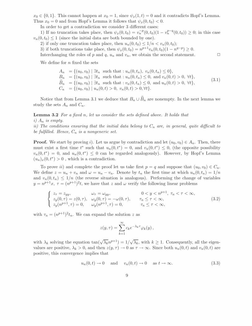
First, we take p = 1, q = 1/3 and initial conditions u0 = 1 + x and v0 = 1 + x − x2. Weobtain the following pictures for the approximate problem with n = 100.

0 0.2 0.4 0.6 0.8 1−0.4

−0.2

0

0.2

0.4

0.6

0.8

1

un(0,t)

vn(0,t)

11

0

0.5

1

0

0.5

1−0.5

0

0.5

1

1.5

2

u component

0

0.5

1

0

0.5

10

0.5

1

1.5

v component

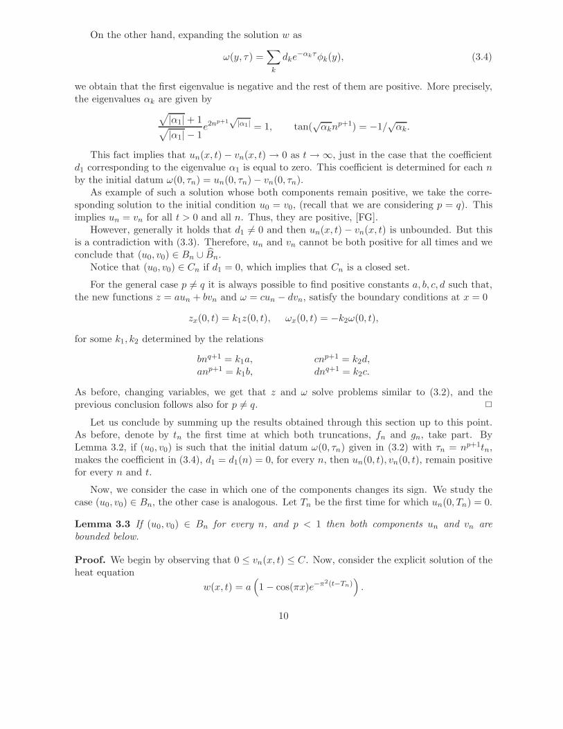
We can observe that the v component converges to the mean value of v(x, T ) as t → ∞(it is a solution to the heat equation with homogeneous Neumann boundary data), while the ucomponent goes to −∞ (it is a solution to the heat equation with boundary flux (vn)−p(0, t)).Also it can be observed that the time derivative of both components at x = 0 becomes verylarge at times t ≈ T .

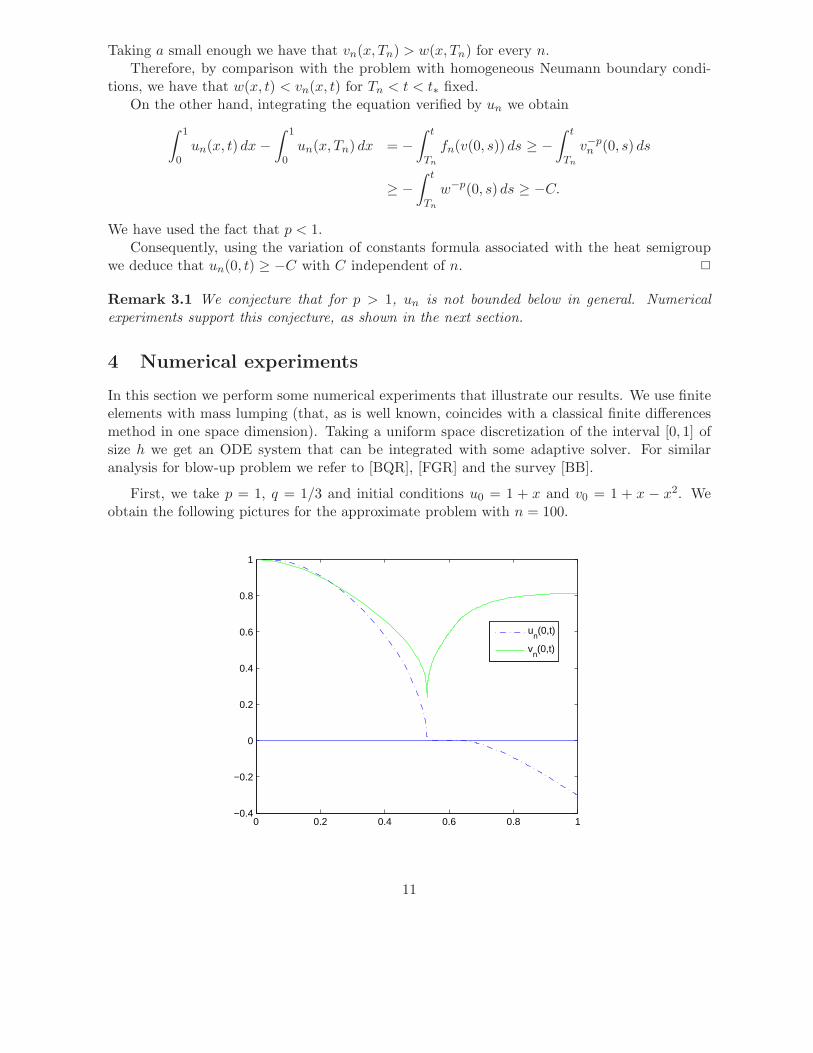
Next, we take p = q = 1/3 and u0 = v0 = 1 + x. In this case we have u(x, t) = v(x, t) andtherefore simultaneous quenching with continuation given by a solution to the Dirichlet problem.We remark again that this case is not generic.

0 0.5 1 1.5 2 2.5 30

0.2

0.4

0.6

0.8

1

1.2

un(0,t)

0

0.5

10

1

2

3

0

0.5

1

1.5

2

tx

u

These pictures illustrate the Dirichlet condition taken by the limit after T .

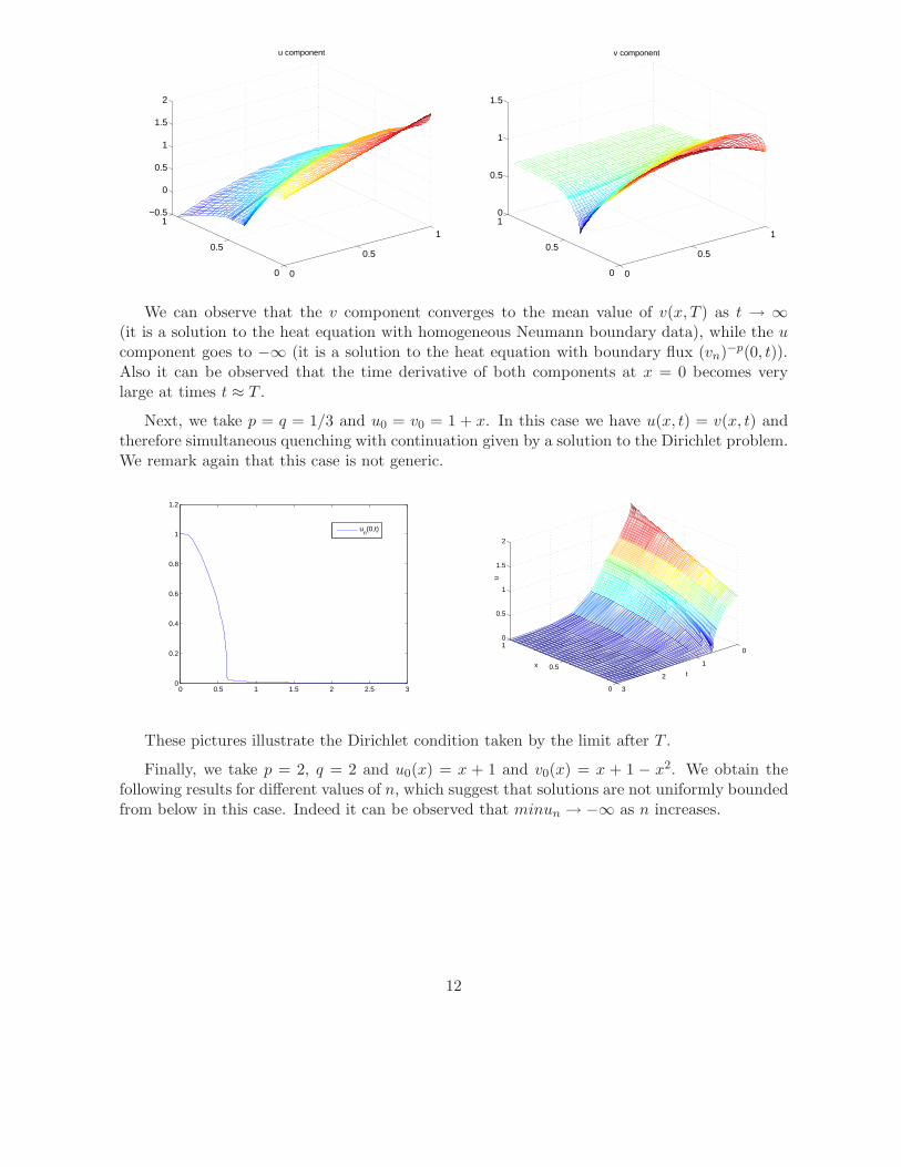
Finally, we take p = 2, q = 2 and u0(x) = x + 1 and v0(x) = x + 1 − x2. We obtain thefollowing results for different values of n, which suggest that solutions are not uniformly boundedfrom below in this case. Indeed it can be observed that minun → −∞ as n increases.

12

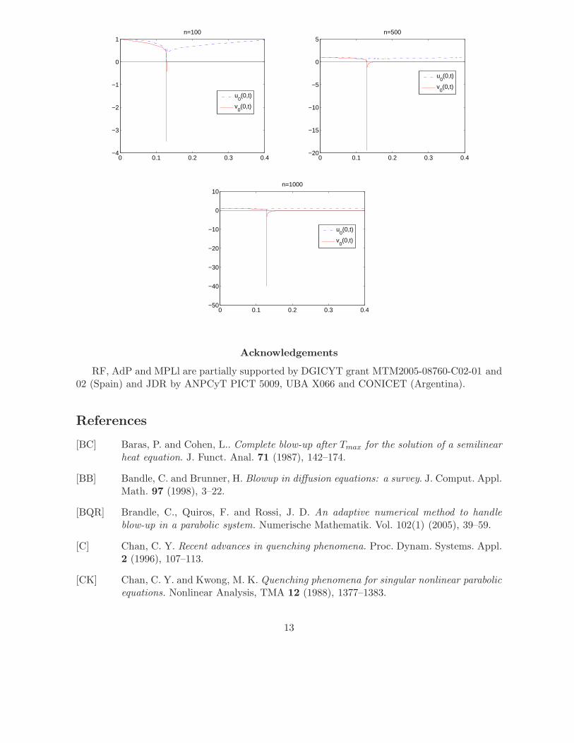
0 0.1 0.2 0.3 0.4−4

−3

−2

−1

0

1n=100

u0(0,t)

v0(0,t)

0 0.1 0.2 0.3 0.4−20

−15

−10

−5

0

5n=500

u0(0,t)

v0(0,t)

0 0.1 0.2 0.3 0.4−50

−40

−30

−20

−10

0

10n=1000

u0(0,t)

v0(0,t)

Acknowledgements

RF, AdP and MPLl are partially supported by DGICYT grant MTM2005-08760-C02-01 and02 (Spain) and JDR by ANPCyT PICT 5009, UBA X066 and CONICET (Argentina).

References

[BC] Baras, P. and Cohen, L.. Complete blow-up after Tmax for the solution of a semilinearheat equation. J. Funct. Anal. 71 (1987), 142–174.

[BB] Bandle, C. and Brunner, H. Blowup in diffusion equations: a survey. J. Comput. Appl.Math. 97 (1998), 3–22.

[BQR] Brandle, C., Quiros, F. and Rossi, J. D. An adaptive numerical method to handleblow-up in a parabolic system. Numerische Mathematik. Vol. 102(1) (2005), 39–59.

[C] Chan, C. Y. Recent advances in quenching phenomena. Proc. Dynam. Systems. Appl.2 (1996), 107–113.

[CK] Chan, C. Y. and Kwong, M. K. Quenching phenomena for singular nonlinear parabolicequations. Nonlinear Analysis, TMA 12 (1988), 1377–1383.

13

[DX] Deng, K. and Xu, M. Quenching for a nonlinear diffusion equation with a singularboundary condition. Z. Angew. Math. Phys. 50 (1999), 574–584.

[FGR] Ferreira, R., Groisman, P. and Rossi, J. D. Numerical blow-up for a nonlinear problemwith a nonlinear boundary condition. Math. Mod. Meth. Appl. Sci. 12(4) (2002), 461–484.

[FPQR] Ferreira, R., de Pablo, A., Quiros, F. and Rossi, J. D. Non-simultaneous quenching ina system of heat equations coupled at the boundary. Z. Angew. Math. Phys. 57 (2006),no. 4, 586–594.

[FG] Fila, M., and Guo, J. S.Complete blow-up and incomplete quenching for the heatequation with a nonlinear boundary condition. Nonlinear Anal. 48 (2002), no. 7, 995–1002.

[FL] Fila, M. and Levine, H. A. Quenching on the boundary. Nonlinear Anal. 21 (1993),795–802.

[GV1] Galaktionov, V. A. and Vazquez, J. L. Necessary and sufficient conditions for completeblow-up and extinction for one-dimensional quasilinear heat equations. Arch. RationalMech. Anal. 129 (1995), 225–244.

[GV2] Galaktionov, V. A. and Vazquez, J. L. Continuation of blowup solutions of nonlinearheat equations in several space dimensions. Comm. Pure Appl. Math. 50 (1997), 1–67.

[K] Kawarada, H. On solutions of initial-boundary problem for ut = uxx +1/(1−u). Publ.Res. Inst. Math. Sci. 10 (1974/75), no. 3, 729–736.

[KN] Ke, L. and Ning, S. Quenching for degenerate parabolic equations. Nonlinear Anal. 34(1998), 1123–1135.

[L] Levine, H. A. Quenching and beyond: a survey of recent results. GAKUTO Internat.Ser. Math. Sci. Appl. 2 (1993) , Nonlinear mathematical problems in industry II ,Gakkotosho, Tokyo, 501–512.

[L2] Levine, H. A. The phenomenon of quenching: a survey. In “Trends in the Theory andPractice of Nonlinear Analysis”, (V. Lakshmikantham, ed.), Elsevier Science Publ.,North Holland, 1985, pp. 275–286.

[L3] Levine, H. A. The quenching of solutions of nonlinear parabolic and hyperbolic equa-tions with nonlinear boundary conditions. SIAM J. Math. Anal. 14 (1983), 1139–1153.

[PQR] de Pablo, A., Quiros, F. and Rossi, J. D. Nonsimultaneous quenching. Appl. Math.Lett. 15 (2002), no. 3, 265–269.

[QR1] Quiros, F. and Rossi, J. D. Non-simultaneous blow-up in a semilinear parabolic system.Z. Angew. Math. Phys. 52 (2001), no. 2, 342–346.

[QR2] Quiros, F. and Rossi, J. D. Non-simultaneous blow-up in a nonlinear parabolic system.Adv. Nonlinear Stud. 3 (2003), no. 3, 397–418.

14

[QRV] Quiros, F., Rossi, J. D. and Vazquez, J. L. Thermal avalanche for blow-up solutionsof semilinear heat equations. Comm. Pure Appl. Math. LVII, (2004), 59–98.

[ST] Souplet, P and Tayachi, S. Optimal condition for non-simultaneous blow-up in areaction-diffusion system. J. Math. Soc. Japan 56 (2004), no. 2, 571–584.

15