Counting in The Wild - University of Oxfordvgg/publications/2016/Arteta16/arteta… · counting accuracy over a baseline density-based counting approach, and obtains comparable accuracy

Counting in The Wild

Carlos Arteta1, Victor Lempitsky2, and Andrew Zisserman1

1Department of Engineering Science, University of Oxford, UK2Skolkovo Institute of Science and Technology (Skoltech), Russia

Abstract. In this paper we explore the scenario of learning to countmultiple instances of objects from images that have been dot-annotatedthrough crowdsourcing. Specifically, we work with a large and challengingimage dataset of penguins in the wild, for which tens of thousands ofvolunteer annotators have placed dots on instances of penguins in tensof thousands of images. The dataset, introduced and released with thispaper, shows such a high-degree of object occlusion and scale variationthat individual object detection or simple counting-density estimation isnot able to estimate the bird counts reliably.To address the challenging counting task, we augment and interleavedensity estimation with foreground-background segmentation and ex-plicit local uncertainty estimation. The three tasks are solved jointly bya new deep multi-task architecture. Using this multi-task learning, weshow that the spread between the annotators can provide hints about lo-cal object scale and aid the foreground-background segmentation, whichcan then be used to set a better target density for learning density predic-tion. Considerable improvements in counting accuracy over a single-taskdensity estimation approach are observed in our experiments.

1 Introduction

This paper is motivated by the need to address a challenging large-scale real-world image-based counting problem that cannot be tackled well with exist-ing approaches. This counting task arises in the course of ecological surveysof Antarctic penguins, and the images are automatically collected by a set offixed cameras placed in Antarctica with the intention of monitoring the penguinpopulation of the continent. The visual understanding of the collected imagesis compounded by many factors such as the variability of vantage points ofthe cameras, large variation of penguin scales, adversarial weather conditions inmany images, high similarity of the appearance between the birds and some ele-ments in the background (e.g. rocks), and extreme crowding and inter-occlusionbetween penguins (Figure 1).

The still ongoing annotation process of the dataset consists of a public web-site [27], where non-professional volunteers annotate images by placing dots ontop of individual penguins; this is similar to citizen science annotators, who havealso been used as an alternative to paid annotators for vision datasets (e.g. [19]).The simplest form of annotation (dotting) was chosen to scale up the annotationprocess as much as possible. Based on the large number of dot-annotated im-ages, our goal is to train a deep model that can solve the counting task throughdensity regression [4, 6, 8, 16, 25, 26].

2 C. Arteta, V. Lempitsky and A. Zisserman

Compared to the training annotations used in previous works on density-based counting, our crowd-sourced annotations show abundant errors and con-tradictions between annotators. We therefore need to build models that can learnin the presence of noisy labels. Perhaps, an even bigger challenge than annota-tion noise, is the fact that dot annotations do not directly capture informationabout the characteristic object scale, which varies wildly in the dataset (the di-ameter of a penguin varies between ∼15 and ∼700 pixels). This is in contrastto previous density estimation methods that also worked with (less noisy) dotannotations but assumed that the object scale was either constant or could beinferred from a given ground plane estimate.

To address the challenges discussed above, we propose a new approach forlearning to count that extends the previous approaches in several ways. Ourfirst extension over density-based methods is the incorporation of an explicitforeground-background segmentation into the learning process. We found thatwhen using noisy dot annotations, it is much easier to train a deep networkfor foreground-background segmentation than for density prediction. The keyinsight is that once such a segmentation network is learned, the predicted fore-ground masks can be used to form a better target density function for learningthe density prediction.

Also, the density estimates predicted for new images can be further combinedwith the foreground segmentation, e.g. by setting the density in the backgroundregions to zero.

Our second extension is to take advantage of the availability of multipleannotations in two ways. First, by exploiting the spatial variations across theannotations, we obtain cues towards the scale of the objects. Second, by exploit-ing also their counting variability, we add explicit prediction of the annotationdifficulty into our model. Algorithmically, while it is possible to learn the net-works for segmentation and density estimation in sequence, we perform jointfine-tuning of the three components corresponding to object-density prediction,foreground-background segmentation, and local uncertainty estimation, using adeep multi-task network.

This new architecture enables us to tackle the very hard counting problem athand. Careful analysis suggests that the proposed model significantly improves incounting accuracy over a baseline density-based counting approach, and obtainscomparable accuracy to the case when the depth information is available.

2 Background

Counting objects in crowded scenes. Parsing crowded scenes, such as thecommon example of monitoring crowds in surveillance videos, is a challengingtask mainly due to the occlusion between instances in the crowd, which cannot beproperly resolved by traditional binary object detectors. As a consequence, mod-els emerged which cast the problem as one where image features were mappedinto a global object count [2, 3, 7], or local features mapped into pixel-wise objectdensities [4, 6, 8, 16, 24, 26] which can be integrated into the object count over

Counting in The Wild 3

any image region. In either case, these approaches provided a way to obtain anobject count while avoiding detecting the individual instances. Moreover, if thedensity map is good enough, it has been shown that it can be used to provide anestimate for the localization of the object instances [1, 11]. The task in this workis in practice very similar to the pixel-wise object density estimation from localfeatures, and also executed using convolutions neural networks (CNN) similar to[16, 24, 26]. However, aside from the main differences in the underlying statisti-cal annotation model, our model differs from previous density learning methodsin that we use a CNN architecture mainly designed for the segmentation task,in which the segmentation mask is used to aid the regression of the density map.Our experiments demonstrate the importance of such aid.

Learning from multiple annotators. The increasing amount of availabledata has been a key factor in the recent rapid progress of the learning-basedcomputer vision. While the data collection can be easily automated, the bottle-neck in terms of cost and effort mostly resides in the data annotation process.Two complementary strategies help the community to alleviate this problem: theuse of crowds for data annotation (e.g. through crowdsourcing platforms suchas Amazon Mechanical Turk); and the reduction in the level of difficulty of suchannotations (e.g. image-level annotations instead of bounding boxes). Indeed,both solutions create in turn additional challenges for the learning models. Forexample, crowdsourced annotations usually show abundant errors, which createthe necessity of building models that can learn in the presence of noisy labels.Similarly, dealing with simpler annotations demands more complex models, suchas in learning to segment from image-level labels instead of pixel-level annota-tions, where the model also needs to infer on its own the difference between theobject and the background. Nevertheless, regardless of the added complexity,coping with simpler and/or noisy supervision while taking advantage of vastamounts of data is a scalable approach.

Dealing with multiple annotators has been generally approached by mod-elling different annotation variables with the objective of scoring and weightingthe influence of each of the annotators [12, 22, 23], and finding the ground-truthlabel that is assumed to exist in the consensus of the annotators [10, 14, 21].However, in cases such as the penguin dataset studied in this paper, most ofthe annotations are performed by tens of thousands of different and mostlyanonymous users, each of which provides a very small set of annotations, thusreducing the usefulness of modelling the reliabilities of individual annotators.Moreover, ambiguous examples are extremely common in such crowded and oc-cluded scenes, which not only means that it is often not possible to agree ona ground-truth, but also that the errors of the individual annotators, most no-tably missing instances in the counting case, can be so high that a ground-truthcannot be determined from the annotations alone as all of them are far fromit. On the positive side, the variability between annotators is proportional tothe image difficulty, thus we chose to learn to predict directly the uncertainty oragreement of the annotators, and not only the most likely instance count. There-fore, we argue that providing a confidence band for the object count still fulfils


the objective of the counting task, taking advantage of the multiple annotators.We note that this predictive uncertainty is different from the uncertainty in themodel parameters, which could also be determined from a learned architecturesimilar to the one used in this work (e.g. [5]), but that is not used here. Instead,the approach taken in this paper is more similar to [23] where uncertainty of theannotator is directly used in the learning model, although it is determined bythe annotator recording their uncertainty in the annotation system, as opposedto deriving it from the disagreement between annotators.

Learning from dot-annotations. Dot annotations are an easy way to labelimages, but generally require additional cues in order to be used in learningcomplex tasks. For example, [15] showed how to use dots in combination withan objectness prior in order to learn segmentations from images that wouldotherwise only have image-level labels. Dots have also been used in the contextof interactive segmentation [18, 20] with cues such as background annotations,which are easy to provide in an interactive context. The most common taskin which dot-annotations are used is that of counting [1, 4, 8, 25], where theyare used in combination with direct information about the spatial extent of theobject in order to define object density maps that can be regressed. However,in all of these cases the dots are introduced by a single annotator. We showthat when dot annotations are crowdsourced, and several annotators label eachimage, the required spatial cues can be obtained from the point patterns, whichcan then be used for object density estimation or segmentation.

3 The penguin dataset

The penguin dataset [13] is a product of an ongoing project for monitoring thepenguin population in Antarctica. The images are collected by a series of fixedcameras in over 40 different sites, which collect images every hour. Examples canbe seen in Figure 1. The data collection process has been running for over threeyears, and has produced over 500 thousand images with resolutions between 1MPand 6MP. The image resolution in combination with the camera shots, translateinto penguin sizes ranging from under 15 pixels to over 700 pixels in length.

Among the information that the zoologists wish to extract from these data, akey piece is the trend in the size of the population of penguins on each site, whichcan then be studied for correlation with different factors such as climate change.Therefore, it is necessary to obtain the number of penguins present in each ofthe frames. The goal of making this dataset available to the vision community isto contribute to the development of a framework that can accurately parse thiscontinuous stream of images.

So far, the annotation process of the dataset has been carried out by humanvolunteers in a citizen science website [27], where any person can enter to placedots inside the penguins appearing in the image. Currently, the annotation toolhas received over 35 thousand different volunteers. Once an image has beenannotated by twenty volunteers, it is removed from the annotation site.


Max Count: 35 Max Count: 38

Max Count: 28 Max Count: 130

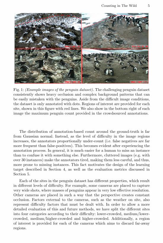
Fig. 1: (Example images of the penguin dataset). The challenging penguin datasetconsistently shows heavy occlusion and complex background patterns that canbe easily mistaken with the penguins. Aside from the difficult image conditions,the dataset is only annotated with dots. Regions of interest are provided for eachsite, shown in this figure with red lines. We also show in the bottom right of eachimage the maximum penguin count provided in the crowdsourced annotations.

The distribution of annotation-based count around the ground-truth is farfrom Gaussian normal. Instead, as the level of difficulty in the image regionsincreases, the annotators proportionally under-count (i.e. false negatives are farmore frequent than false-positives). This becomes evident after experiencing theannotation process. In general, it is much easier for a human to miss an instancethan to confuse it with something else. Furthermore, cluttered images (e.g. withover 30 instances) make the annotators tired, making them less careful, and thus,more prone to missing instances. This fact motivates the design of the learningtarget described in Section 4, as well as the evaluation metrics discussed inSection 5.

Each of the sites in the penguin dataset has different properties, which resultin different levels of difficulty. For example, some cameras are placed to capturevery wide shots, where masses of penguins appear in very low effective resolution.Other cameras are placed in such a way that the perspective creates constantocclusion. Factors external to the cameras, such as the weather on site, alsorepresent difficulty factors that must be dealt with. In order to allow a moredetailed evaluation of this and future methods, we have split the different sitesinto four categories according to their difficulty: lower-crowded, medium/lower-crowded, medium/higher-crowded and higher-crowded. Additionally, a regionof interest is provided for each of the cameras which aims to discard far-awayregions.


Input and dot-annotations

Labels for segmentation

Segmentation map s(p)

Labels for density

Density map λ(p)

Labels for uncertainty

Uncertainty map u(p)

Task I Task II – From s(p) Task III

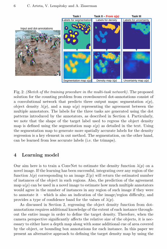
Fig. 2: (Sketch of the training procedure in the multi-task network). The proposedsolution for the counting problem from crowdsourced dot-annotations consist ofa convolutional network that predicts three output maps: segmentation s(p),object density λ(p), and a map u(p) representing the agreement between themultiple annotators. The labels for the three tasks are generated using the dotpatterns introduced by the annotators, as described in Section 4. Particularly,we note that the shape of the target label used to regress the object densitymap is defined using the segmentation map s(p) as detailed in the text. Usingthe segmentation map to generate more spatially accurate labels for the densityregression is a key element in out method. The segmentation, on the other hand,can be learned from less accurate labels (i.e. the trimaps).

4 Learning model

Our aim here is to train a ConvNet to estimate the density function λ(p) on anovel image. If the learning has been successful, integrating over any region of thefunction λ(p) corresponding to an image I(p) will return the estimated numberof instances of the object in such regions. Also, the prediction of the agreementmap u(p) can be used in a novel image to estimate how much multiple annotatorswould agree in the number of instances in any region of such image if they wereto annotate it – which is also an indication of the image/region difficulty, andprovides a type of confidence band for the values of λ(p).

As discussed in Section 2, regressing the object density function from dot-annotations requires additional knowledge of the extent of each instance through-out the entire image in order to define the target density. Therefore, when thecamera perspective significantly affects the relative size of the objects, it is nec-essary to either have a depth map along with some additional cue of area coveredby the object, or bounding box annotations for each instance. In this paper wepresent an alternative approach to defining the target density map by using the


object (foreground) segmentation, as this can be an easier task to learn with lesssupervision than the density regression. We present such an approach with andwithout any depth information, preceded by an overview of the general learningarchitecture.

Learning architecture. The learning architecture is a multi-task convolutionalneural network which aims to produce (i) a foreground/background segmentations(p), (ii) an object density function λ(p), and (iii) a prediction of the agreementbetween the annotators u(p) as a measure of uncertainty. While the usual mo-tivation for the use of multi-task architectures is the improvement in the gener-alization, here we additionally reuse the predicted segmentations to change theobjective for other branches as learning progresses.

The segmentation branch consists of a pixel-wise binary classification pathwith a hinge loss. For the second task of regressing λ(p), where more precisepixel-wise values are required, we use the segmentation mask s(p) from the firsttask as a prior. That is, the target map for learning λ(p) is constructed from an

approximation λ(p) that is built using the class segmentation s(p). The densitytarget map is regressed with a root-mean-square loss. Finally, the same regressionloss function is used in the third and final branch of the CNN in order to predicta map u(p) of agreement between the annotators, as described below.

Labels for learning. A fundamental aspect of this framework is the way thelabels are defined for the different learning tasks based on the multiple dotannotations. The details will depend on the specific model used, described laterin Section 4.1 and Section 4.2, but we fist introduce the general aspects of them.Given a set of dots D = d1, d2, . . . , dK , we define a trimap t(p) of ‘positive’,‘negative’ and ‘ignore’ regions, which respectively are likely to correspond toregions mostly contained inside instances of the object, regions corresponding tobackground, and uncertain regions in between. Example trimaps are shown inFigure 3.

Regression targets. A key aspect is defining the regression target for each taskas this in turn defines the pixel-wise loss. For the segmentation map target, thepositive and negative regions in the trimap are used to define the foregroundand background pixel labels, whereas the ignore regions do not contribute inthe computation of the pixel classification loss (i.e. the derivatives of the lossin those spatial locations are set to zero for the backpropagation through theCNN). As the network learns to regress this target, the predicted foregroundregions can extend beyond the positives of the trimap into the ignore regions tobetter match the true foreground/background segmentation, as can be seen inFigure 2.

The density map target is obtained from the predicted segmentation and theuser annotations. First, connected components are obtained from the predictedsegmentation. Then, for each connected component, an integer score is assignedas the maximum over the different annotators. We pick the maximum as a wayto counter-balance the consistent under-estimation of the count (e.g. as opposedto the mean) as discussed in Section 3. The density target is defined for eachpixel of the connected component by assigning it the integer score divided by


the component area (so that integrating the density target over the componentarea gives the maximum annotation).

Finally, the uncertainty map target for annotator (dis)agreement consist ofthe variance of the annotations within each of the connected component regions.More principled ways of handling the annotation bias along with the uncertaintyare briefly discussed in Section 6 (applicable to crowdsourced dot-annotations ingeneral), but we initially settle for the more practical MAX and VAR approachesdescribed above.

Implementation details. The core of the CNN is the segmentation architec-ture FCN8s presented in [9], which is initialized from the VGG-16 [17] classifi-cation network, and adds skip and fusion layers for a finer prediction map whichcan be evaluated at the scale of the input image.

We make extensive use of scaling-based data augmentation while trainingthe ConvNet by up-scaling each image to six different scales and taking randomcrops of 700 × 700 pixels, our standard input size while training. This is donewith the intention of gaining the scale invariance required in the counting task(i.e. the spatial region in the density map corresponding to a single penguinshould sum to one independently of its size in pixels).

We train for the three tasks in parallel and end-to-end. The overall weightof the segmentation loss is set to be higher than the remaining two losses as wewant this easier task to have more influence over the filters learned; we foundthat this helps to avoid the divergence of the learning that could happen duringthe iterations where the segmentation prior is far from local optima. At the startof the training it is necessary to provide an initial target for the density map loss,since the segmentation map s(p) is not yet defined. Again the trimap is used,but more loosely here than in the segmentation target, with the union of thepositive and ignore maps used to define the connected components. The densityis then obtained by assigning annotations to the connected components in thesame manner as used during training. At the end of this initialization the densitytarget will generally spread beyond the objects since it includes the ignore region.The initial trimap can be estimated in two different ways depending on whetherthe rough estimate of depth information is available. We now discuss these twocases.

4.1 Learning from multiple dot-annotations and depth information

We wish to use the dot-annotations provided by multiple annotators for animage to generate a trimap t(p) for that image. The trimap will be used for theintermediate learning step of a segmentation mask s(p).

Due to perspective effects the penguins further from the camera are smaller,and this typically means that penguins become smaller moving from the bottomto the top of the image for the camera placements used in our dataset. Weassume here that we have a depth map for the scene, together with an estimateof the object class size (e.g. penguins are roughly of a similar real size), and thuscan predict the size of a penguin at any point in the image.


Subset of dot-annotations

Distance transform

Kernel density estimate

Trimap

Trimap

With depth

Without depth

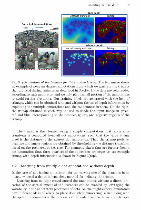
Fig. 3: (Generation of the trimaps for the training labels). The left image showsan example of penguin dataset annotations from which we generate the trimapsthat are used during training, as described in Section 4; the dots are color-codedaccording to each annotator, and we only plot a small portion of the annotationsto avoid further cluttering. Our training labels are generated with the help oftrimaps, which can be obtained with and without the use of depth information byexploiting the multiple annotations and the randomness in them. On the right,the trimap obtained in each way is used to shade the input image in green,red and blue, corresponding to the positive, ignore, and negative regions of thetrimap.

The trimap is then formed using a simple computation: first, a distancetransform is computed from all dot annotations, such that the value at anypixel is the distance to the nearest dot annotation. Then the trimap positive,negative and ignore regions are obtained by thresholding the distance transformbased on the predicted object size. For example, pixels that are further from adot annotation than three quarters of the object size are negative. An exampletrimap with depth information is shown in Figure 3(top).

4.2 Learning from multiple dot-annotations without depth

In the case of not having an estimate for the varying size of the penguins in animage, we need a depth-independent method for defining the trimap.

Learning from multiple crowdsourced dot annotations without a direct indi-cation of the spatial extent of the instances can be enabled by leveraging thevariability in the annotators placement of dots. As one might expect, annotatorshave different ideas of where to place dots when annotating, which along withthe spatial randomness of the process, can provide a sufficient cue into the spa-


tial distribution of each instance. The more annotators are available, the betterthe spatial cue can get.

We harness this spatial distribution by converting it into a density functionρ(p), and then thresholding ρ(p) at two levels to obtain the positive, ignoreand negative regions of the trimap t(p). The density is simply computed byplacing a Gaussian kernel with bandwidth h at each provided dot annotation:ρ(p) =

∑Nj=1

1hK(

p−dj

h ) where d1...dN is the set of provided points. We note thatthis can be seen as a generalization of the approach for generating the targetdensity map used in previous counting work for the case of a single annotatorand a Gaussian kernel [1].

The only question remaining is how to determine the size of the Gaussiankernel h. We rely on a simple heuristic to extract from the dot-patterns a cue forthe selection of h: annotations on a larger instance tend to be more distributedthan annotations on smaller objects. In fact, the relation between point patterndistribution and object size is not a clear one as it is affected by other factors suchas occlusion, but it is sufficient for our definition. The estimation of h consistsof doing a rough reconciliation of the dot patterns from multiple annotators (todetermine which dots should be assigned to the same penguin), followed by thecomputation of a single value of h that suits an entire image. The reconciliationprocess is done by matching the dots between pairs of annotators using theHungarian algorithm, with a matching cost given by Euclidean distance. Thisproduces a distribution of distances between dots that are likely to belong to thesame instance. After combining all pairs of annotators, h is then taken to be themedian of this distribution of distances. An illustration of ρ(p) can be seen inFigure 3(bottom) using a Gaussian kernel, which we keep for our experimentsof Section 5.

Finally, the trimap t(p) is obtained from ρ(p) by thresholding as above. Ascan be seen in Figure 3(bottom), this approach has less information than usingdepth and results in slightly worse trimaps (i.e. with more misplaced pixels),which in our experiments translate to slower convergence of the learning.

5 Experiments

Metrics for counts from crowdsourced dot-annotations. As discussed inSection 3, benchmarking on the penguin dataset is a challenging task due tothe lack of ground-truth. Moreover, it is a common case in the penguin datasetthat the true count, under any reasonable definition, might lie far from what theannotators have indicated, and is generally an under-estimation. Therefore, wepropose to evaluate the performance on this dataset using metrics that not onlyreflect the similarity of the automatic estimations w.r.t. what the annotatorsintroduced, but also the uncertainty in them; ultimately, both aspects are usefulinformation regarding the image.

Considering the under-counting bias of the annotators, we firstly propose tocompare with a region-wise max of the annotations. That is, we first define aset of “positive” regions based on the dot-annotations, as done in the learning


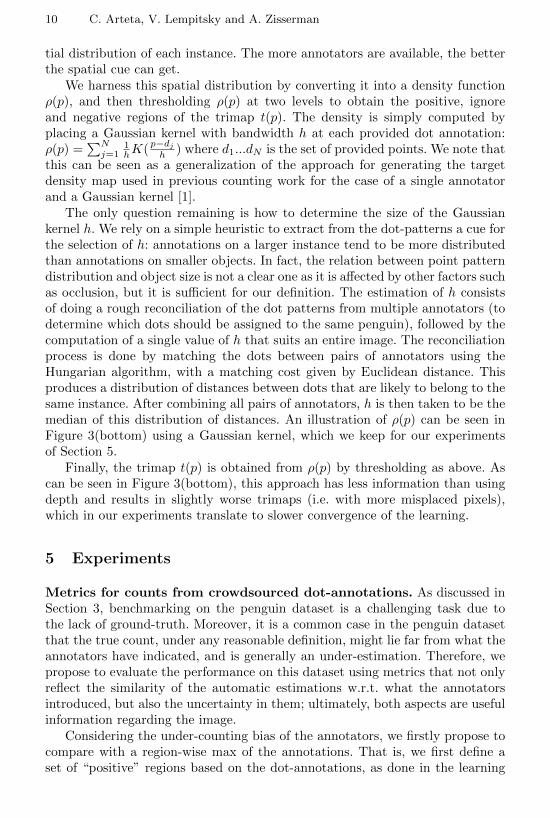
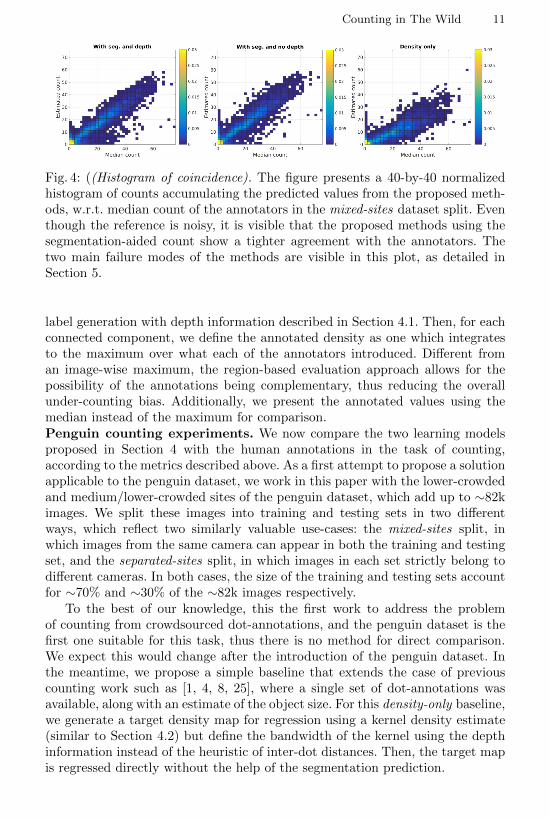
Fig. 4: ((Histogram of coincidence). The figure presents a 40-by-40 normalizedhistogram of counts accumulating the predicted values from the proposed meth-ods, w.r.t. median count of the annotators in the mixed-sites dataset split. Eventhough the reference is noisy, it is visible that the proposed methods using thesegmentation-aided count show a tighter agreement with the annotators. Thetwo main failure modes of the methods are visible in this plot, as detailed inSection 5.

label generation with depth information described in Section 4.1. Then, for eachconnected component, we define the annotated density as one which integratesto the maximum over what each of the annotators introduced. Different froman image-wise maximum, the region-based evaluation approach allows for thepossibility of the annotations being complementary, thus reducing the overallunder-counting bias. Additionally, we present the annotated values using themedian instead of the maximum for comparison.Penguin counting experiments. We now compare the two learning modelsproposed in Section 4 with the human annotations in the task of counting,according to the metrics described above. As a first attempt to propose a solutionapplicable to the penguin dataset, we work in this paper with the lower-crowdedand medium/lower-crowded sites of the penguin dataset, which add up to ∼82kimages. We split these images into training and testing sets in two differentways, which reflect two similarly valuable use-cases: the mixed-sites split, inwhich images from the same camera can appear in both the training and testingset, and the separated-sites split, in which images in each set strictly belong todifferent cameras. In both cases, the size of the training and testing sets accountfor ∼70% and ∼30% of the ∼82k images respectively.

To the best of our knowledge, this the first work to address the problemof counting from crowdsourced dot-annotations, and the penguin dataset is thefirst one suitable for this task, thus there is no method for direct comparison.We expect this would change after the introduction of the penguin dataset. Inthe meantime, we propose a simple baseline that extends the case of previouscounting work such as [1, 4, 8, 25], where a single set of dot-annotations wasavailable, along with an estimate of the object size. For this density-only baseline,we generate a target density map for regression using a kernel density estimate(similar to Section 4.2) but define the bandwidth of the kernel using the depthinformation instead of the heuristic of inter-dot distances. Then, the target mapis regressed directly without the help of the segmentation prediction.


With segmentation and depth With segmentation and no depth

1.4 ± 0.15.0 ± 1.5

0.7 ± 0.0

0.7 ± 0.1

1.0 ± 0.1

1.9 ± 0.3 2.4 ± 0.40.9 ± 0.0

0.6 ± 0.0

0.8 ± 0.11.0 ± 0.1

0.9 ± 0.1

5.9 ± 1.90.8 ± 0.3

1.7 ± 0.6

2.8 ± 1.5 2.7 ± 1.60.9 ± 0.2

0.3 ± 0.1

0.9 ± 0.40.9 ± 0.4

0.2 ± 0.0

1.0 ± 0.2 0.1 ± 0.0

59.7 ± 22.6

0.1 ± 0.0

0.4 ± 0.4 0.1 ± 0.0

62.1 ± 51.6

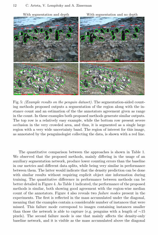
Fig. 5: (Example results on the penguin dataset). The segmentation-aided count-ing methods proposed outputs a segmentation of the region along with the in-stance count and an estimation of the the annotators agreement given as rangein the count. In these examples both proposed methods generate similar outputs.The top row is a relatively easy example, while the bottom row present severeocclusion in the very crowded area, and thus, it is segmented as a single largeregion with a very wide uncertainty band. The region of interest for this image,as annotated by the penguinologist collecting the data, is shown with a red line.

The quantitative comparison between the approaches is shown in Table 1.We observed that the proposed methods, mainly differing in the usage of anauxiliary segmentation network, produce lower counting errors than the baselinein our metrics and different data splits, while being very similar in performancebetween them. The latter would indicate that the density prediction can be donewith similar results without requiring explicit object size information duringtraining. The quantitative difference in performance between methods can bebetter detailed in Figure 4. As Table 1 indicated, the performance of the proposedmethods is similar, both showing good agreement with the region-wise mediancount of the annotators. Figure 4 also reveals two failure modes present in theexperiments. The first is reflected in the mass accumulated under the diagonal,meaning that the examples contain a considerable number of instances that weremissed. This failure mode correspond to images containing instances smallerthan those the network is able to capture (e.g. penguins with a length of ∼15pixels). The second failure mode is one that mainly affects the density-onlybaseline network, and it is visible as the mass accumulated above the diagonal


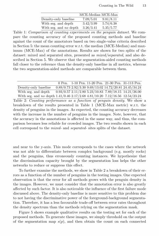
MCE-Median MCE-Max

Density-only baseline 7.09/5.01 9.81/8.11

With seg. and depth 3.42/3.99 5.74/6.38With seg. and no depth 3.26/3.41 5.35/5.77

Table 1: Comparison of counting experiments on the penguin dataset. We com-pare the counting accuracy of the proposed counting methods and baselineagainst the count of the annotators based on two single-value criteria describedin Section 5: the mean counting error w.r.t. the median (MCE-Median) and max-imum (MCE-Max) of the annotations. Results are shown for two splits of thedataset: mixed and separated sites, presented as mixed/separated, and also de-scribed in Section 5. We observe that the segmentation-aided counting methodsfall closer to the reference than the density-only baseline in all metrics, whereasthe two segmentation-aided methods are comparable between them.

0 Pen. 1-10 Pen. 11-20 Pen. 21-30 Pen. 31-113 Pen.

Density-only baseline 0.89/0.73 2.92/3.30 9.69/13.02 14.72/20.81 24.45/34.24

With seg. and depth 0.93/0.57 2.11/2.80 5.23/10.83 7.89/18.15 14.21/26.00With seg. and no depth 1.41/0.46 2.17/2.68 4.81/10.20 7.12/16.56 12.54/23.24

Table 2: Counting performance as a function of penguin density. We show abreakdown of the results presented in Table 1 (MCE-Max metric) w.r.t. thedensity of penguins in the images. As expected, the counting accuracy decreaseswith the increase in the number of penguins in the images. Note, however, thatthe accuracy in the annotations is affected in the same way, and thus, the com-parison becomes less reliable for crowded images. The two results shown in eachcell correspond to the mixed- and separated- sites splits of the dataset.

and near to the y-axis. This mode corresponds to the cases where the networkwas not able to differentiate between complex background (e.g. mostly rocks)and the penguins, thus erroneously counting instances. We hypothesize thatthe discrimination capacity brought by the segmentation loss helps the othernetworks to reduce or suppress this effect.

To further examine the methods, we show in Table 2 a breakdown of their er-rors as a function of the number of penguins in the testing images. One expectedobservation is that the error for all methods grows with the penguin density inthe images. However, we must consider that the annotation error is also greatlyaffected by such factor. It is also noticeable the influence of the first failure modediscussed above. The density-only baseline is more sensitive to this problem dueto not having the discriminative power of the foreground-background segmenta-tion. Therefore, it has a less favourable trade-off between error rates throughoutthe density spectrum than the methods relying on the segmentation mask.

Figure 5 shows example qualitative results on the testing set for each of theproposed methods. To generate these images, we simply threshold on the outputof the segmentation map s(p), and then obtain the count on each connected


component by integrating the corresponding region over the density map λ(p).Finally, we add the learned measure of annotator uncertainty u(p) as a boundfor the estimated count. Qualitatively, both methods obtain similar results re-gardless of their training differences. Further examples are available at [13].Effect of the number of annotators. Finally, we examine how the perfor-mance of the proposed counting method is affected by the number of annotatorsin the training images. In the previous experiments we used all images that hadat least five annotators, with an average of 8.8. Instead, we now perform thetraining with the same set of images but limiting the number of annotators todifferent thresholds; the testing set is kept the same as before. The experimentwas done on the variant of our method that uses the site depth information (withseg. and depth in Table 1), and taking three random subsets of the annotators foreach image. The results using the MCE-max metric were 7.12±0.20, 6.37±0.25and 6.14±0.29 when limiting the number of annotators to 1, 3 and 5 respectively.We recall that the MCE-max was 5.74 when using all the annotators available.This experiment confirms an expected progressive improvement in the countingaccuracy as the number of annotators per image increases.

6 Discussion

We have presented an approach that is designed to address a very challengingcounting task on a new dataset with noisy annotations done by citizen scien-tists. We augment and interleave density estimation with foreground-backgroundsegmentation and explicit local uncertainty estimation. All three processes areembedded into a single deep architecture and the three tasks are solved by jointtraining. As a result, the counting problem (density estimation) benefits from therobustness that the segmentation task has towards noisy annotation. Curiously,we show that the spread between the annotators can in some circumstances helpimage analysis by providing a hint about the local object scale.

While we achieve a good counting accuracy in our experiments, many chal-lenges remain to be solved. In particular, better models are required for uncer-tainty estimation and for crowdsourced dot-annotations. The current somewhatunsatisfactory method (using MAX and VAR as targets in training) could bereplaced with a quantitative model of the uncertainty, e.g. using GeneralizedExtreme Value distributions to model the crowdsourced dot-annotations, withtheir consistent under-counting. Alternatively, dot-annotations could be mod-elled more formally as a spatial point processes with a rate function λ(p). Inaddition, a basic model of crowdsourced dot-annotations is required in orderto better disentangle errors related to the estimation model, from those errorsarising from the noisy annotations.Acknowledgements. We thank Dr. Tom Hart and the Zooniverse team for their

leading role in the penguin watch project. Financial support was provided by theRCUK Centre for Doctoral Training in Healthcare Innovation (EP/G036861/1) andthe EPSRC Programme Grant Seebibyte EP/M013774/1.

References

[1] Arteta, C., Lempitsky, V., Noble, J.A., Zisserman, A.: Interactive object counting.In: ECCV (2014)

[2] Chan, A.B., Liang, Z.S.J., Vasconcelos, N.: Privacy preserving crowd monitoring:Counting people without people models or tracking. In: CVPR (2008)

[3] Chan, A.B., Vasconcelos, N.: Bayesian poisson regression for crowd counting. In:CVPR (2009)

[4] Fiaschi, L., Nair, R., Koethe, U., Hamprecht, F.: Learning to count with regressionforest and structured labels. In: ICPR (2012)

[5] Gal, Y., Ghahramani, Z.: Dropout as a bayesian approximation: Representingmodel uncertainty in deep learning. arXiv preprint arXiv:1506.02142 (2015)

[6] Idrees, H., Soomro, K., Shah, M.: Detecting humans in dense crowds using locally-consistent scale prior and global occlusion reasoning. Pattern Analysis and Ma-chine Intelligence, IEEE Transactions on (2015)

[7] Kong, D., Gray, D., Tao, H.: A viewpoint invariant approach for crowd counting.In: ICPR (2006)

[8] Lempitsky, V., Zisserman, A.: Learning to count objects in images. In: NIPS (2010)[9] Long, J., Shelhamer, E., Darrell, T.: Fully convolutional networks for semantic

segmentation. In: CVPR (2015)[10] Ma, F., Li, Y., Li, Q., Qiu, M., Gao, J., Zhi, S., Su, L., Zhao, B., Ji, H., Han, J.:

Faitcrowd: Fine grained truth discovery for crowdsourced data aggregation. In:Proceedings of the 21th ACM SIGKDD International Conference on KnowledgeDiscovery and Data Mining. ACM (2015)

[11] Ma, Z., Yu, L., Chan, A.B.: Small instance detection by integer programming onobject density maps. In: CVPR (2015)

[12] Ouyang, R.W., Kaplan, L.M., Toniolo, A., Srivastava, M., Norman, T.: Paralleland streaming truth discovery in large-scale quantitative crowdsourcing. IEEETransactions on Parallel and Distributed Systems (2016)

[13] Penguin research webpage, www.robots.ox.ac.uk/∼vgg/research/penguins[14] Raykar, V.C., Yu, S., Zhao, L.H., Valadez, G.H., Florin, C., Bogoni, L., Moy, L.:

Learning from crowds. The Journal of Machine Learning Research (2010)[15] Russakovsky, O., Bearman, A.L., Ferrari, V., Li, F.F.: What’s the point: Semantic

segmentation with point supervision. arXiv preprint arXiv:1506.02106 (2015)[16] Shao, J., Kang, K., Loy, C.C., Wang, X.: Deeply learned attributes for crowded

scene understanding. In: CVPR (2015)[17] Simonyan, K., Zisserman, A.: Very deep convolutional networks for large-scale im-

age recognition. In: International Conference on Learning Representations (2015)[18] Straehle, C., Koethe, U., Hamprecht, F.A.: Weakly supervised learning of image

partitioning using decision trees with structured split criteria. In: ICCV (2013)[19] Van Horn, G., Branson, S., Farrell, R., Haber, S., Barry, J., Ipeirotis, P., Perona,

P., Belongie, S.: Building a bird recognition app and large scale dataset with citizenscientists: The fine print in fine-grained dataset collection. In: CVPR (2015)

[20] Wang, T., Han, B., Collomosse, J.: Touchcut: Fast image and video segmentationusing single-touch interaction. Computer Vision and Image Understanding (2014)

[21] Welinder, P., Branson, S., Perona, P., Belongie, S.J.: The multidimensional wisdomof crowds. In: NIPS (2010)


[22] Whitehill, J., Wu, T.f., Bergsma, J., Movellan, J.R., Ruvolo, P.L.: Whose voteshould count more: Optimal integration of labels from labelers of unknown exper-tise. In: NIPS (2009)

[23] Wolley, C., Quafafou, M.: Learning from multiple naive annotators. In: AdvancedData Mining and Applications. Springer (2012)

[24] Xie, W., Noble, J.A., Zisserman, A.: Microscopy cell counting with fully con-volutional regression networks. In: MICCAI 1st Workshop on Deep Learning inMedical Image Analysis (2015)

[25] Xie, W., Noble, J.A., Zisserman, A.: Microscopy cell counting and detection withfully convolutional regression networks. Computer Methods in Biomechanics andBiomedical Engineering: Imaging & Visualization (2016)

[26] Zhang, C., Li, H., Wang, X., Yang, X.: Cross-scene crowd counting via deep con-volutional neural networks. In: CVPR (2015)

[27] Zooniverse: penguinwatch.org

Documents

Counting in The Wild - University of Oxfordvgg/publications/2016/Arteta16/arteta… · counting accuracy over a baseline density-based counting approach, and obtains comparable accuracy