Calibrating photon-counting detectors to high

accuracy: background and deadtime issues

Michael Ware∗ Alan Migdall†, Joshua C. Bienfang‡, and Sergey V. Polyakov†,∗Brigham Young University, Provo, UT

†Optical Technology Div., NIST, Gaithersburg, MD‡Electron and Optical Physics Div., NIST, Gaithersburg, MD

May 4, 2006

Abstract

When photon-counting detectors are calibrated in the presence of abackground signal, deadtime effects can be significant and must be care-fully accounted for to achieve high accuracy. We present a method forseparating the correlated signal from the background signal that appro-priately handles deadtime effects. This method includes consideration ofpulse timing and afterpulsing issues that arise in typical avalanche photodiode (APD) detectors. We illustrate how these effects should be ac-counted for in the calibration process. We also discuss detector timingissues that should be considered in detector calibration.

Keywords: Photon counting; Quantum metrology; Single photon detectors;

1 Introduction

The photon pairs produced in parametric down-conversion provide a fundamen-tally absolute way to calibrate single photon detectors [1–14]. Because the pho-tons are produced in pairs, the detection of one photon heralds with certaintythe existence of the other. To measure detection efficiency, a trigger detectionsystem is placed to intercept some of the down-converted light. The detectorunder test (DUT) is then arranged to collect all the photons correlated to thoseseen by the trigger detector (and usually more). In the ideal case, the DUTchannel detection efficiency is the ratio of the number of coincidence events tothe number of trigger detection events in a given time interval. (By ideal casehere, we mean that other than the two-photon source, there are no competingmechanisms causing the detectors to fire and by coincidence we mean that thetwo detectors fire due to the two photons of a pair.) If we specify the collectionefficiency of the DUT and trigger channels by ηDUT and ηtrig, respectively, thenthe total number of trigger counts is

Ntrig = ηtrigNp (1)

1

and the total number of coincidence counts is

Nc = ηDUTηtrigNp, (2)

where Np is the total number of down-converted photons emitted into the triggerchannel during the counting period. The absolute detection efficiency of theDUT channel is then simply

ηDUT =Nc

Ntrig

. (3)

Note that this is the efficiency of the entire detection channel (including collec-tion optics, etc.) and not just the efficiency of the DUT alone [15, 16].

A number of groups have pursued detector calibration using this method (seeRef. [15] for a more detailed history). We are currently pursing an experimentwhere we hope to achieve calibration uncertainties on the 0.1% level. To achievethis level of uncertainty, we must carefully consider how the idealized calibrationsetup described above is actually implemented in the laboratory. In this articlewe describe some subtle effects that arise from non-ideal measurement devices,and illustrate how they can be handled to achieve low uncertainties.

An accurate experimental determination of Ntrig is usually straightforward:the electronic detector signals are summed during the counting period, and thendarkcounts and counts due to background photons are estimated and subtractedoff. Experimental techniques for making these estimates are detailed in Ref. [16].

Determining NC accurately requires significantly more effort. In a typicalcalibration setup, NC is determined by making a histogram of the delays betweentrigger and DUT detection events (see Figure 1a). In this setup the photonsproduced simultaneously are sent to two avalanche photodiode (APD) photon-counting modules, one designated as trigger and one as DUT. The trigger andDUT detector module outputs are sent to the start and stop inputs respectivelyof a time digitizing circuit that records the arrival time of each pulse. Theelectronic signal of the DUT is delayed with an appropriate length of cable toassure that that the DUT (stop) pulse arrives at the time digitizing circuit afterthe trigger (start) pulse.

The histogram in Fig. 1a records the delay between each DUT event andthe most recent trigger event. The principal coincidence peak (A) is evidentin the histogram at a delay of 55 ns, and to first approximation, the numberof coincidences NC can be estimated as the sum of events in this peak, withthe background subtracted off. However, a more accurate determination of thenumber of coincidences requires an understanding of the smaller peaks (E) at13 ns, (F) at 34 ns, and (D) at 98 ns. Moreover, it is not immediately clearwhat background to subtract because the levels are different on either side ofthe main peak. The difference in background levels is due to detector deadtime,and becomes more pronounced in situations where the DUT has high detectionefficiency and the background count rate is high. In these situations, the simplebackground subtraction technique introduces small errors because it does notaccount for deadtime effects. In this paper we illustrate how to properly han-dle histogram data when calibrating high efficiency detectors in the presence of

2

high background rates. While the corrections to the simple background sub-traction technique are small, they can be relevant when calibrating detectors tohigh precision. We also discuss timing and afterpulsing issues that arise whenconsidering a histogram like the one in Fig. 1a.

2 Histogram Features

To correctly calibrate the detector, we must first consider all of the features(peaks, backgrounds, valleys, etc.) and determine their origins. Then we canseparate ‘heralded’ photon events from background events. To illustrate thisprocess, we consider the data in Fig. 1a. The main coincidence peak (A) is themost prominent feature of the histogram and obviously represents correlatedevents. The origin of the small ‘shoulder’ (labeled B) on the right the maincoincidence peak is a little less obvious. In section 4 we will see that this shoulderrepresents valid, but delayed, coincidence counts, and we will discuss why theyare delayed. The broad dip (labeled C) to the right of the peak is due to detectordeadtime. Since the detector is most likely to receive a photon at a delay of≈ 55 ns, it is also likely to be ‘dead’ for a finite duration at subsequent delaysand thus is unable to register the arrival of background photons. This behaviorcomplicates the process of separating background events from correlated events.In section 3 we discuss how to to properly separate the two types of events inthe presence of deadtime.

Peak D is due to afterpulsing in the DUT. The APDs in our setup are activelyquenched (i.e. the bias voltage is reduced to below the APD breakdown voltage)for ≈ 42 ns after an event is registered. When the quenching ends, there is asmall probability that the detector will produce a false pulse (referred to as anafterpulse). The size of this peak indicates that an afterpulse is registered for≈ 1% of the pulses in the main coincidence peak. We will discuss the structureof the afterpulse in section 4.

The tiny peaks labeled E and F are specific to our particular setup. PeakE is produced by afterpulsing of the trigger detector. Because we have delayedthe arrival of the DUT pulses ≈ 55 ns longer than the trigger pulses, the af-terpulses of the trigger arrive before the correlated DUT pulses. Because wemeasure the delay between DUT pulses and the most recent trigger pulse, thisresults in a small coincidence peak 42 ns before the main peak. These are validcoincidences, although they make only a tiny correction to the final detectionefficiency (≈ 0.1% of peak A) in the situation shown. This peak could have beeneliminated by simply adjusting the delay lines so that the main coincidence peakoccurred at a delay less than 42 ns (or ignoring trigger pulses that occur tooclose to the previous trigger). We chose to leave the setup as shown to helpillustrate the other effects discussed below.

Peak F is also simply understood. In our setup, we couple trigger photonsinto a fiber and then couple the output of the fiber onto the trigger APD.There is a small back-reflection at either end of the fiber, and photons thatexperience a back-reflection at both ends of the fiber arrive at the APD after

3

traveling two extra fiber lengths. Our fiber is 2 m long and this extra double-pass corresponds to a delay of ≈ 20 ns. Again, the coincidences in this peak arevalid, and account for ≈ 0.1% of the total coincidence counts. Eliminating, orantireflection coating, the fiber in the trigger detection path would remove thispeak, but we left it in our setup for convenience and to illustrate things thatshould be considered in a high accuracy detector calibration.

3 Separating Background from Signal

When high efficiency detectors are calibrated in situations with high backgroundcount rates, the simple background subtraction method discussed earlier in-troduces errors in the estimation of detector efficiency. For a more accuratetreatment, we use a probabilistic treatment of the data to separate backgroundevents from events correlated to the trigger.

We begin with a measured histogram denoted by H(τi), where τi denotesthe time delay for the ith bin. As usual, the histogram records the cumulativenumber of detection events received in each bin. The number of histogramtrigger pulses (i.e. histogram starts) received while accumulating the histogramis specified by T . Our goal is to separate the events represented by H(τi) intotwo categories: events correlated to the trigger pulse and background events.Formally, we write

H(τi) = Cm(τi) + Bm(τi), (4)

where Cm(τi) and Bm(τi) denote, respectively, the number of correlated andbackground events recorded in a given bin. The subscript ‘m’ reminds us thatthese quantities represent the number of correlated and background events thatwere actually measured in each bin. In a calibration, efficiency can be defined anumber of ways. Here, we define it as how many correlated events would have

been measured if the detector were ‘live’ (ready for a detection) each time acorrelated photon was incident on the system. This number will be larger thanthe simple estimate of efficiency Cm/T , since the detector may be dead when thecorrelated photon arrives due to a previous background count. In addition, thebackground rate may not be a simple constant due to previous background orcorrelated events (recall that this is the origin of the dip labeled C in Fig. 1(a)).

We consider a simple model of detector deadtime where the detector is ‘dead’for d time bins after registering an event (where d is an integer), and thenimmediately becomes ‘live’ again. For ease of notation, we will assume that thedelay of the DUT channel has been chosen long enough that all of the correlatedsignal appears after the dth histogram bin.1 This requires that

Cm(τi) = 0 (i ≤ d). (5)

1The specification that all correlated signal occurs after d bins is, of course, artificial andintroduced only for notational convenience. In practice, it is usually easier just to recordthe correlated signal and then pad the leading portion of the histogram with some extrabackground rather than using extra long DUT delays.

4

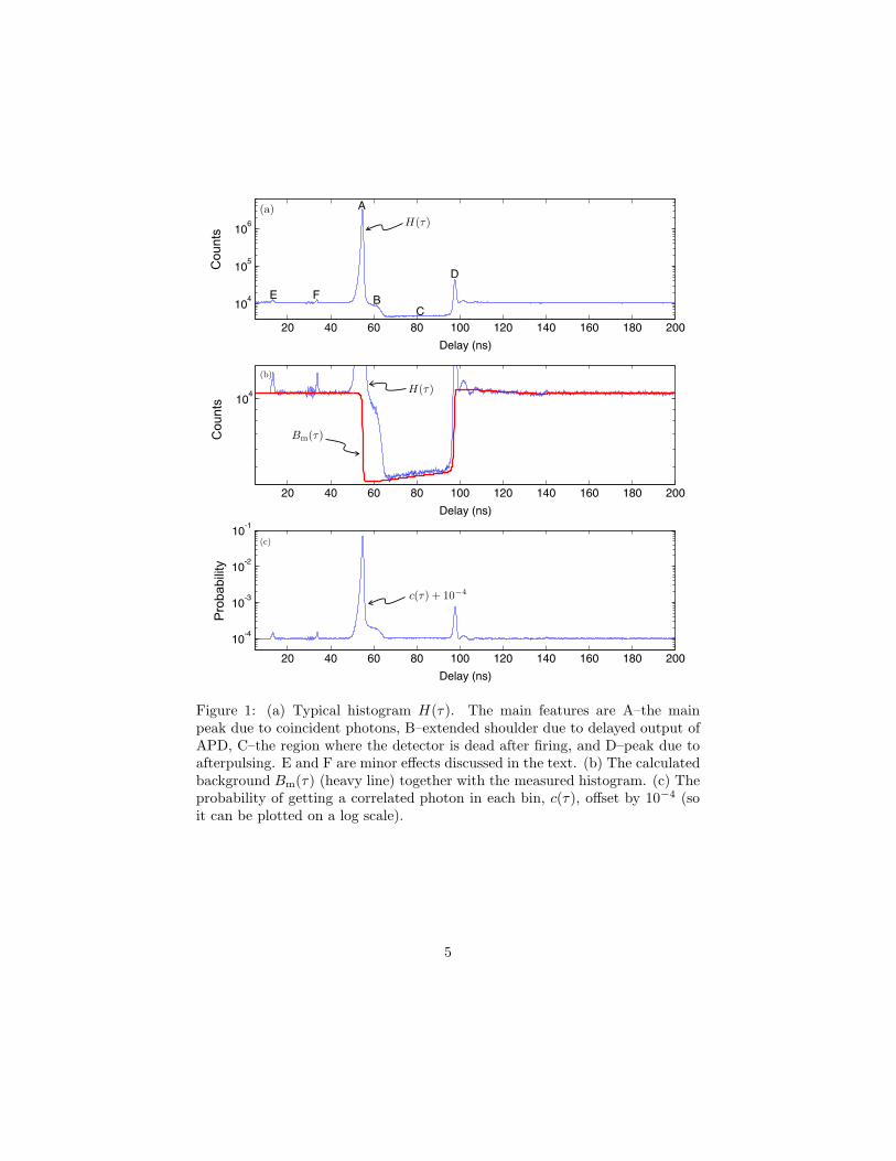
Figure 1: (a) Typical histogram H(τ). The main features are A–the mainpeak due to coincident photons, B–extended shoulder due to delayed output ofAPD, C–the region where the detector is dead after firing, and D–peak due toafterpulsing. E and F are minor effects discussed in the text. (b) The calculatedbackground Bm(τ) (heavy line) together with the measured histogram. (c) Theprobability of getting a correlated photon in each bin, c(τ), offset by 10−4 (soit can be plotted on a log scale).

5

We also assume that the mean number of background events in a given bin isconstant before correlated events arrive, and define B0 as the average number ofbackground events/bin recorded in bins with i < d. Using B0, we can calculatethe probability b that a background event could be measured in a bin (duringa given scan) assuming that the detector was alive at that moment. In theabsence of correlated signal, this is simply

B0 = b × (T − dB0). (6)

The value in parenthesis of Eq. (6) gives the total number of times that it waspossible to record an event in the bin (i.e. the total number of scans minus thenumber of scans where the detector was dead due to a background event in oneof the previous d bins).

We can also write an expression for b in the presence of correlated signal. Inthis case we have

Bm(τi) = b ×

T −

i−1∑

j=i−d

H(τj) − ∆(τi)

(i ≥ d). (7)

As before, the number in parenthesis is the number of scans where it was possibleto record a background event in the bin. The sum gives the number of timesthat the detector was dead in the ith bin due to a background or signal eventsin one of the previous d bins. The function ∆(τi) accounts for the situationswhere a trigger pulses resets the delay before it reaches the ith bin. (Recallthat we histogram DUT events with respect to the most recent trigger event.)Since the trigger detector also experiences deadtime, ∆(τi) is equal to zero forthe first d bins of the histogram. After that, ∆(τi) grows with τi (linearly tofirst approximation). It is usually a simple matter to extract ∆(τi) from themeasured histogram.

We can combine Eqs. (6) and (7) to write a convenient expression for Bm(τi)in terms of measured quantities:

Bm(τi) =B0

T − dB0

×

T −

i−1∑

j=i−d

H(τj) − ∆(τi)

(i > d). (8)

To evaluate this equation, we need Bm(τi) for i ≤ d. Since we have specifiedthat there is no correlated signal and ∆(τi) = 0 in this region of the histogram,we have Bm(τi) = H(τi) ≈ B0, (i ≤ d). Figure 1b shows Bm(τ) calculatedfor the histogram in Fig. 1a together with H(τ) for comparison. Note thatour definition of b does not distinguish between a background event and anafterpulse of a background event, which results in slight underestimation of thebackground during the dead region in Fig. 1(b), however such underestimationresults in ≈ 0.03% error in the final overall detector efficiency.2

2To introduce a simple correction for afterpulses due to uncorrelated events, one couldassume that the number of afterpulses in the histogram bin i is proportional to the numberof events in the bin (i − d) with a constant probability of an afterpulse β, i.e. by addingβH(τi−d) to the righthand sides of Eqs. (6) and (7); β can be determined as a ratio of peaksD and A.

6

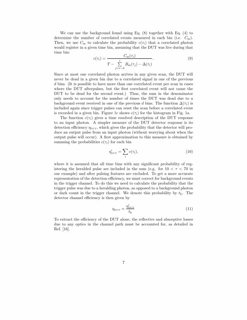
We can use the background found using Eq. (8) together with Eq. (4) todetermine the number of correlated events measured in each bin (i.e. Cm).Then, we use Cm to calculate the probability c(τi) that a correlated photonwould register in a given time bin, assuming that the DUT was live during thattime bin:

c(τi) =Cm(τi)

T −i

∑

j=i−d

Bm(τj) − ∆(τi)

. (9)

Since at most one correlated photon arrives in any given scan, the DUT willnever be dead in a given bin due to a correlated signal in one of the previousd bins. (It is possible to have more than one correlated event per scan in caseswhere the DUT afterpulses, but the first correlated event will not cause theDUT to be dead for the second event.) Thus, the sum in the denominatoronly needs to account for the number of times the DUT was dead due to abackground event received in one of the previous d bins. The function ∆(τi) isincluded again since trigger pulses can reset the scan before a correlated eventis recorded in a given bin. Figure 1c shows c(τi) for the histogram in Fig. 1a.

The function c(τi) gives a time resolved description of the DUT responseto an input photon. A simpler measure of the DUT detector response is itsdetection efficiency ηDUT, which gives the probability that the detector will pro-duce an output pulse from an input photon (without worrying about when theoutput pulse will occur). A first approximation to this measure is obtained bysumming the probabilities c(τi) for each bin

η′

DUT=

∑

i

c(τi), (10)

where it is assumed that all time bins with any significant probability of reg-istering the heralded pulse are included in the sum (e.g. for 10 < τ < 70 inour example) and after pulsing features are excluded. To get a more accuraterepresentation of the detection efficiency, we must correct for background eventsin the trigger channel. To do this we need to calculate the probability that thetrigger pulse was due to a heralding photon, as opposed to a background photonor dark count in the trigger channel. We denote this probability by th. Thedetector channel efficiency is then given by

ηDUT =η′

DUT

th(11)

To extract the efficiency of the DUT alone, the reflective and absorptive lossesdue to any optics in the channel path must be accounted for, as detailed inRef. [16].

7

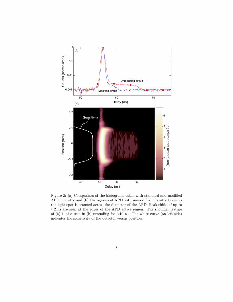
Figure 2: (a) Comparison of the histograms taken with standard and modifiedAPD circuitry and (b) Histograms of APD with unmodified circuitry taken asthe light spot is scanned across the diameter of the APD. Peak shifts of up to≈2 ns are seen at the edges of the APD active region. The shoulder featureof (a) is also seen in (b) extending for ≈10 ns. The white curve (on left side)indicates the sensitivity of the detector versus position.

8

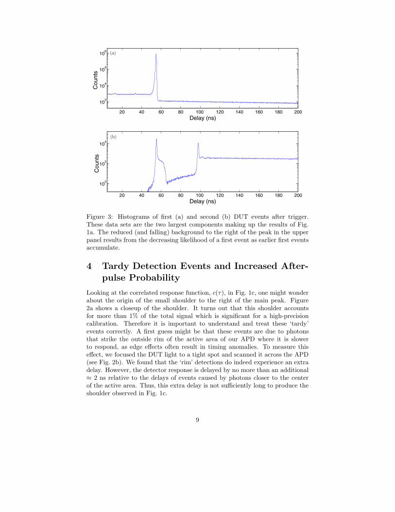
Figure 3: Histograms of first (a) and second (b) DUT events after trigger.These data sets are the two largest components making up the results of Fig.1a. The reduced (and falling) background to the right of the peak in the upperpanel results from the decreasing likelihood of a first event as earlier first eventsaccumulate.

4 Tardy Detection Events and Increased After-

pulse Probability

Looking at the correlated response function, c(τ), in Fig. 1c, one might wonderabout the origin of the small shoulder to the right of the main peak. Figure2a shows a closeup of the shoulder. It turns out that this shoulder accountsfor more than 1% of the total signal which is significant for a high-precisioncalibration. Therefore it is important to understand and treat these ‘tardy’events correctly. A first guess might be that these events are due to photonsthat strike the outside rim of the active area of our APD where it is slowerto respond, as edge effects often result in timing anomalies. To measure thiseffect, we focused the DUT light to a tight spot and scanned it across the APD(see Fig. 2b). We found that the ‘rim’ detections do indeed experience an extradelay. However, the detector response is delayed by no more than an additional≈ 2 ns relative to the delays of events caused by photons closer to the centerof the active area. Thus, this extra delay is not sufficiently long to produce theshoulder observed in Fig. 1c.

9

To get more information about these tardy pulses, we separated the his-togram events by the order in which they were received after the trigger (i.e.the first event after a trigger, the second event after the trigger, etc.). Figure 3ashows the distribution of first events, and Fig. 3b shows the distribution of sec-ond events. As would be expected, the main coincidence peak consists primarilyof first events, and the afterpulse peak is composed of second events. Note thatthe shoulder of tardy coincidence events (located at 57–62 ns) also consists ofsecond DUT events. Since the DUT deadtime is ≈ 42 ns, this means that thetardy coincidence events were registered right after the detector had recoveredfrom a previous avalanche recorded during the first 15–20 ns of the histogram.The first avalanche in this case is due to a background (as opposed to a corre-lated) event. This suggests that the timing of DUT pulses can be influenced byprevious detection events (if they were recent enough). We now consider howthe detector reacts when it receives a photon during its recovery period.

It turns out that the afterpulse probability is not a constant, but can dependon the background rate. This can be explained in terms of the active quenchingcircuitry of the detector. After a detection event, the active quench circuitof the DUT lowers the APD bias voltage to just below breakdown. After thisquench period, the circuit raises the bias back to its original value. At this pointthe APD can avalanche again, and sometimes does so spontaneously causingan ‘afterpulse’. However, if the detector receives a photon during the timeof rising bias, it significantly enhances the probability that the detector willavalanche once the bias returns to its higher value. For higher backgroundrates, it is more likely that a photon will strike the detector during this resetphase and thus increase the likelihood of afterpulses. This is why the probabilityof getting an afterpulse shown in Fig. 1(c) is significantly higher than expectedfrom the APD specification of 0.3%. Interestingly, these ‘twilight’ pulses, whichare triggered by photons arrived during the last moments of the deadtime, aredelayed, sometimes significantly, as compared with ‘normal’ detections.

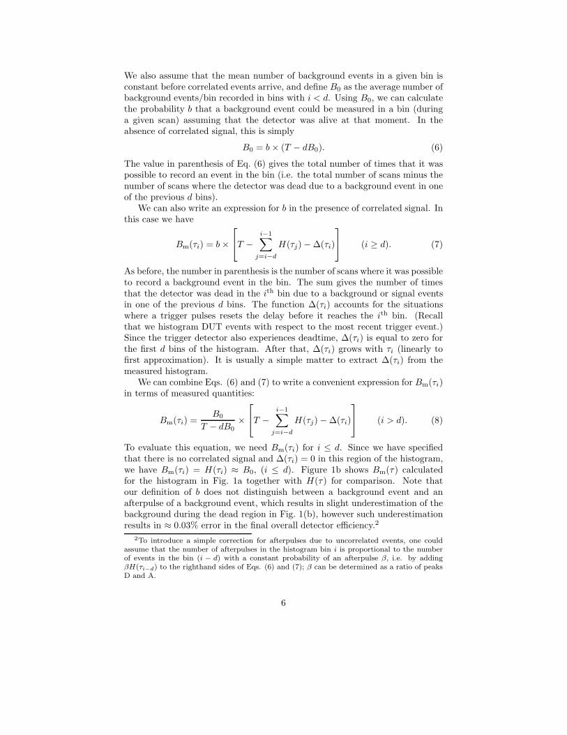
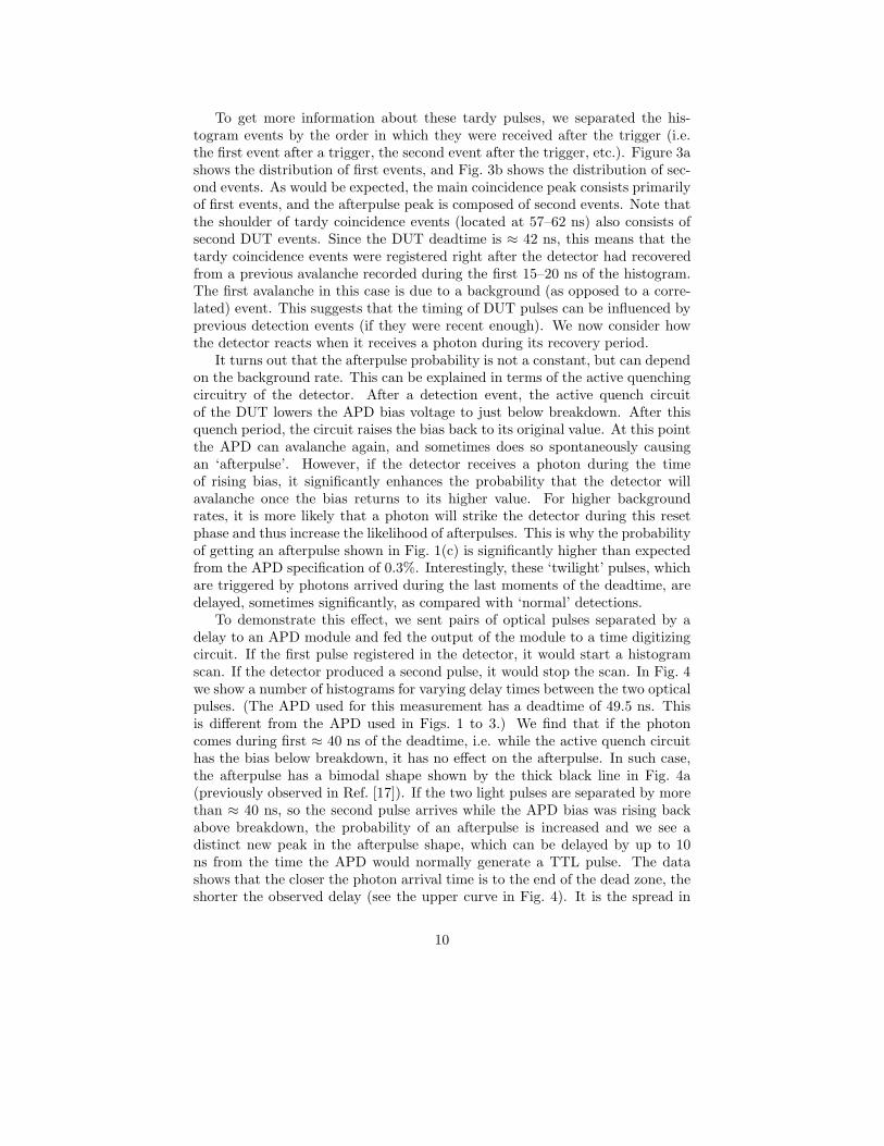
To demonstrate this effect, we sent pairs of optical pulses separated by adelay to an APD module and fed the output of the module to a time digitizingcircuit. If the first pulse registered in the detector, it would start a histogramscan. If the detector produced a second pulse, it would stop the scan. In Fig. 4we show a number of histograms for varying delay times between the two opticalpulses. (The APD used for this measurement has a deadtime of 49.5 ns. Thisis different from the APD used in Figs. 1 to 3.) We find that if the photoncomes during first ≈ 40 ns of the deadtime, i.e. while the active quench circuithas the bias below breakdown, it has no effect on the afterpulse. In such case,the afterpulse has a bimodal shape shown by the thick black line in Fig. 4a(previously observed in Ref. [17]). If the two light pulses are separated by morethan ≈ 40 ns, so the second pulse arrives while the APD bias was rising backabove breakdown, the probability of an afterpulse is increased and we see adistinct new peak in the afterpulse shape, which can be delayed by up to 10ns from the time the APD would normally generate a TTL pulse. The datashows that the closer the photon arrival time is to the end of the dead zone, theshorter the observed delay (see the upper curve in Fig. 4). It is the spread in

10

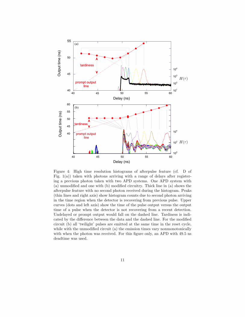
Figure 4: High time resolution histograms of afterpulse feature (cf. D ofFig. 1(a)) taken with photons arriving with a range of delays after register-ing a previous photon taken with two APD systems. One APD system with(a) unmodified and one with (b) modified circuitry. Thick line in (a) shows theafterpulse feature with no second photon received during the histogram. Peaks(thin lines and right axis) show histogram counts due to second photon arrivingin the time region when the detector is recovering from previous pulse. Uppercurves (dots and left axis) show the time of the pulse output versus the outputtime of a pulse when the detector is not recovering from a recent detection.Undelayed or prompt output would fall on the dashed line. Tardiness is indi-cated by the difference between the data and the dashed line. For the modifiedcircuit (b) all ‘twilight’ pulses are emitted at the same time in the reset cycle,while with the unmodified circuit (a) the emission times vary nonmonotonicallywith when the photon was received. For this figure only, an APD with 49.5 nsdeadtime was used.

11

these delays that sets the width of the shoulder feature of Figs. 1 to 3.Interestingly, this feature of the detector can be eliminated with a different

detection circuit. [18] We tested a detector with a modified avalanche detectioncircuit and found that it significantly reduced the late arrival features. Withthat circuit, in Fig. 4 (b) we see the bimodal afterpulse shape has collapsedto a single peak which is consistent with the flat output time line for thosephotons received during the twilight period. This results in the reduction oftardy events as can be seen in Figure 2 (a) which compares a histogram takenwith the modified detector circuit, and one taken with the original active quenchcircuit.

5 Conclusion

We have illustrated how to accurately handle correlated histogram data in cal-ibration situations with a high probability of getting a correlated photon in ascan, and also a non-negligible background rate in the presence of deadtime. Wealso illustrated how other phenomena, such as enhanced detector afterpulsing(and the associated tardy detector output) are due to a high background rate.While these effects are small, they are important to consider when doing highaccuracy calibrations of single-photon-counting detectors. While one may de-fine a detection efficiency as the ideal probability of a live detector producing acount (and only one count) due to a single incident photon, actual implementa-tions are not so clean. In particular, we point out that due to deadtime, tardy,and afterpulse effects, the effective detection efficiency of a photon-counting de-tector is time and history dependent and the final result is an average over aspecific set of conditions. So in cases where a high accuracy overall detection ef-ficiency is required, it is important to understand exactly what those calibrationconditions are and how to apply that result in other situations.

This work was supported in part by the Disruptive Technology Office (DTO)under Army Research Office (ARO) contract number DAAD19-03-1-0199, andDARPA/QUIST.

References

[1] Louisell, W. H., Yariv, A., and Siegman, A. E., 1961, Physical Review, 124,1646–1654.

[2] Zernike, F. and Midwinter, J. E., 1973, Applied Nonlinear Optics, (NewYork: Wiley).

[3] Burnham, D. C. and Weinberg, D. L., 1970, Physical Review Letters, 25,84–87.

[4] Klyshko, D. N., 1977, Soviet Journal of Quantum Electronics, 7, 591–594.

12

[5] Klyshko, D. N., 1981, Soviet Journal of Quantum Electronics, 10, 1112–1116.

[6] Malygin, A. A., Penin, A. N., and Sergienko, A. V., 1981, Soviet Journal

of Quantum Electronics 11, 939–941.

[7] Bowman, S. R., Shih, Y. H., and Alley, C. O., 1986, The use of geiger modeavalanche photodiodes for precise laser ranging at very low light levels: Anexperimental evaluation, Proceeding of SPIE, 663, 24–29.

[8] Rarity, J. G., Ridley, K. D., and Tapster, P. R., 1987, Applied Optics, 26,4616–4619.

[9] Penin, A. N. and Sergienko, A. V., 1991, Applied Optics, 30, 3582–3588.

[10] Ginzburg, V. M., Keratishvili, N., Korzhenevich, E. L., Lunev, G. V.,Penin, A. N., and Sapritsky, V., 1993, Optical Engineering, 32, 2911–2916.

[11] Kwait, P. G., Steinberg, A. M., Chiao, R. Y., Eberhard, P. H., and Petroff,M. D., 1994, Applied Optics, 33, 1844–1853.

[12] Migdall, A., Datla, R., Sergienko, A., Orszak, J. S., and Shih, Y. H., 1995/6,Metrologia, 32, 479–483.

[13] Brida, G., Castelletto, S., Degiovanni, I. P., Novero, C., and Rastello, M. L.,2000, Metrologia, 37, 625–628.

[14] Brida, G., Castelletto, S., Degiovanni, I. P., Genovese, M., Novero, C., andRastello, M. L., 2000, Metrologia, 37, 629–632.

[15] Ware, M. and Migdall, A. L., 2004, Journal of Modern Optics, 15, 1549–1557.

[16] Migdall, A. L., 2001, IEEE Transactions on Intrumentation and Measure-

ment, 50, 478–481.

[17] Spinelli, A., Davis, L. M., and Dautet, H., 1996 “Actively quenched single-photon avalanche diode for high repetition rate time-gated photon count-ing” Rev. Sci. Instrum. 67, 55–61.

[18] Cova, S., Ghioni, M., and Zappa, F. “Circuit for high precision detectionof the time of arrival of photons falling on single photon avalanche diodes,”US Patent 6384663.

13