Correlation between Rotating LIDAR …eces.colorado.edu/~simley/Documents/SimleyPao_AIAA_2013.pdf^u estimate of ucomponent based on lidar measurement azimuth angle in the rotor plane!

Correlation between Rotating LIDAR Measurements

and Blade Effective Wind Speed ∗

Eric Simley† Lucy Y. Pao ‡

Preview wind speed measurements from a forward looking Light Detection and Ranging(LIDAR) system located in the hub of a wind turbine can be used by a feedforward bladepitch control system to mitigate structural loads. For individual blade pitch control, aseparate preview estimate of the effective wind speed encountered by each blade mustbe available. One way of providing an estimate of the blade effective wind speed is toimplement a hub mounted spinning lidar that scans the wind field at the rotational rate ofthe rotor such that the measured wind will reach the blade after some delay. In this way,both the lidar measurement and the wind turbine blade rotationally sample the wind field.The benefit gained by using preview wind speed measurements strongly depends on thecorrelation between the measured wind and the wind that interacts with the blades. Inthis research, the coherence between rotating lidar measurements and blade effective windspeed is calculated and analyzed using a spectral model of the wind field. The simulatedwind field uses an isotropic von Karman spectrum and contains a model of wind evolutiondescribed by a longitudinal spatial coherence function. The coherence between stationarymeasurements and stationary blade effective wind speeds decreases to zero near the 1Protational frequency of the turbine. However, measurement coherence between rotatinglidar measurements and blade effective wind speed remains much higher and does not decayuntil higher frequencies.

Nomenclature

CPSD Cross Power Spectral DensityPSD Power Spectral DensityLIDAR Light Detection and RangingNREL National Renewable Energy Laboratory1P turbine rotational frequencyCQ coefficient of torqueSxx (f) power spectral density of signal xSxy (f) cross power spectral density between signals x and yγ2xy (f) coherence between signals x and yu, v, w longitudinal, transverse, and vertical wind speed components[`x, `y, `z] lidar direction unit vectorueff blade effective wind speedu estimate of u component based on lidar measurementψ azimuth angle in the rotor planeω frequency (rad/s)d measurement preview distanceD longitudinal distance between two pointsf frequency (Hz)

∗This work was supported in part by the US National Renewable Energy Laboratory. Additional industrial support is alsogreatly appreciated.†Doctoral Student, Dept. of Electrical, Computer, and Energy Engineering, University of Colorado, Boulder, CO, Student

Member AIAA.‡Richard and Joy Dorf Professor, Dept. of Electrical, Computer, and Energy Engineering, University of Colorado, Boulder,

CO, Member AIAA.

1 of 15

American Institute of Aeronautics and Astronautics

F lidar focus distanceM number of samples per lidar scan revolutionr scan radius for spinning LIDARU mean wind speed (m/s)

I. Introduction

Combined feedforward/feedback control of wind turbines for structural load mitigation using blade pitchrelies on preview measurements of the wind field disturbance, as shown in Fig. 1. Wind is measured at apreview distance d ahead of the turbine using a Light Detection and Ranging (LIDAR) system, allowingfor d/U seconds of preview, where U is the mean wind speed. The original wind is not measured perfectlyby the lidar but the lidar measurement is used to obtain an estimate of the u, or longitudinal, componentof the wind. As the original upstream wind advects toward the wind turbine at the mean wind speed U ,it typically does not obey Taylor’s frozen turbulence hypothesis,1 but instead evolves, which is commonlydescribed by a coherence loss between points in the wind field separated longitudinally, or in the meanstreamwise direction.2 The feedforward controller is designed to use the preview measurements of the windfield to partially mitigate the effects of the wind disturbance at the rotor. The degree to which variablessuch as structural loads can be reduced using feedforward control depends on the correlation between thewind speed preview measurements and the wind that reaches the rotor.

Figure 1. Block diagram of a combined feedforward/feedback control scenario. The lidar measurement blockrepresents the estimation of the longitudinal component of the wind field given a line-of-sight lidar measure-ment. The wind evolution block represents the coherence loss between wind at the measurement location andthe wind encountered by the rotor after a delay time of d/U . The distance d is the distance upwind of therotor where the measurement is taken and U is the mean wind speed.

Recent research on preview-based feedforward control of wind turbines can be classified as using eithercollective pitch or individual pitch. Collective pitch control requires an estimate of the effective wind speedacross the entire rotor disk to regulate output variables such as rotor speed and tower loads.3 Individualblade pitch control, however, allows for reduction of the loads experienced by each separate blade, whichcould also be transferred to non-rotating components on the turbine.4 Individual pitch control requires moresophisticated measurement of the wind field so that variations throughout the rotor plane can be detected.Research on independent pitch control can be further classified as belonging to one of two categories.5 Con-trollers using a simplified wind field model containing a collective component, vertical shear, and horizontalshear constitute one category.6,7 Multiple lidar measurements are used to form a best-fit estimate of thecollective and shear components to mitigate cyclic loads. This category of individual pitch control works wellin steady winds. However, in a turbulent wind environment the blades experience loads at all frequencies,not just the rotational frequency of the turbine and its harmonics, and a model containing only collectiveand shear components no longer accurately describes the wind field. The second category of individual pitchcontrollers uses a separate preview measurement for each blade.7,8 The lidar measurements are not fit to asimplified model, but are used to control each blade independently. This paper analyzes lidar measurementsfor the latter type of individual pitch control where the correlation between a rotating lidar measurementand the rotating wind speed experienced by a blade, called the blade effective wind speed, is of interest.

2 of 15


The wind speeds that are experienced by the blades as they rotate through the wind field are influencedby rotational sampling of the wind field. Similarly, measurements from a spinning lidar sweeping out acircle ahead of the rotor experience rotational sampling of the wind field. The spectra of a rotationallysampled wind field is very different than the spectra of a wind field sampled at a fixed position. Instead ofexperiencing only the temporal variations in the wind, rotational sampling causes the blades and lidar todetect variations from passing through the spatial structure of the wind field. Due to the effects of rotationalsampling, some energy from low frequencies in the wind field is transferred to the rotational frequency ofthe turbine, known as the 1P frequency, as well as the harmonics thereof.9 In addition, the correlationbetween a spinning lidar measurement, rotating at 1P, and the effective wind speed at a blade benefits fromthe spectral effects of rotational sampling. The spatial averaging effects of both lidar and the varying ofwind speeds across the blade, and the coherence loss due to wind evolution all cause the coherence between astationary preview lidar measurement and a stationary blade effective wind speed to decrease with frequency.However, rotational sampling of the time-varying spatial structures in the wind field causes energy in thehighly correlated low frequencies to concentrate near the 1P frequency and harmonics of the 1P frequency.As a result, rotational measurement coherence remains much higher as frequency increases than stationarymeasurement coherence. The resulting increase in measurement coherence at high frequencies is beneficialfor individual pitch feedforward control.

The rest of this paper is organized as follows. Section II introduces the lidar measurement process, whileblade effective wind speed is defined in Section III. A description of the wind field used is provided inSection IV. Section V discusses the spectra of rotationally sampled wind fields. Results, highlighting theimprovement in correlation between lidar measurements and blade effective wind speeds due to rotationalsampling, are provided in Section VI. Finally, Section VII concludes the paper with a brief discussion.

II. Lidar Measurements

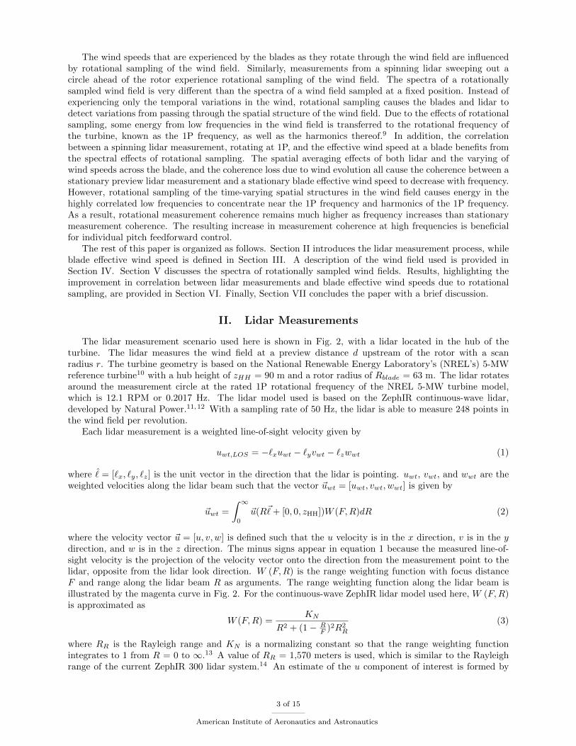
The lidar measurement scenario used here is shown in Fig. 2, with a lidar located in the hub of theturbine. The lidar measures the wind field at a preview distance d upstream of the rotor with a scanradius r. The turbine geometry is based on the National Renewable Energy Laboratory’s (NREL’s) 5-MWreference turbine10 with a hub height of zHH = 90 m and a rotor radius of Rblade = 63 m. The lidar rotatesaround the measurement circle at the rated 1P rotational frequency of the NREL 5-MW turbine model,which is 12.1 RPM or 0.2017 Hz. The lidar model used is based on the ZephIR continuous-wave lidar,developed by Natural Power.11,12 With a sampling rate of 50 Hz, the lidar is able to measure 248 points inthe wind field per revolution.

Each lidar measurement is a weighted line-of-sight velocity given by

uwt,LOS = −`xuwt − `yvwt − `zwwt (1)

where ˆ = [`x, `y, `z] is the unit vector in the direction that the lidar is pointing. uwt, vwt, and wwt are theweighted velocities along the lidar beam such that the vector ~uwt = [uwt, vwt, wwt] is given by

~uwt =

∫ ∞0

~u(R~+ [0, 0, zHH])W (F,R)dR (2)

where the velocity vector ~u = [u, v, w] is defined such that the u velocity is in the x direction, v is in the ydirection, and w is in the z direction. The minus signs appear in equation 1 because the measured line-of-sight velocity is the projection of the velocity vector onto the direction from the measurement point to thelidar, opposite from the lidar look direction. W (F,R) is the range weighting function with focus distanceF and range along the lidar beam R as arguments. The range weighting function along the lidar beam isillustrated by the magenta curve in Fig. 2. For the continuous-wave ZephIR lidar model used here, W (F,R)is approximated as

W (F,R) =KN

R2 + (1− RF )2R2

R

(3)

where RR is the Rayleigh range and KN is a normalizing constant so that the range weighting functionintegrates to 1 from R = 0 to ∞.13 A value of RR = 1,570 meters is used, which is similar to the Rayleighrange of the current ZephIR 300 lidar system.14 An estimate of the u component of interest is formed by

3 of 15


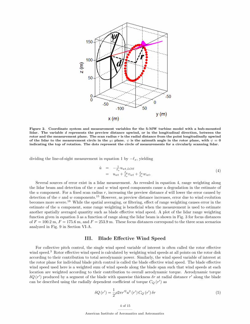
Figure 2. Coordinate system and measurement variables for the 5-MW turbine model with a hub-mountedlidar. The variable d represents the preview distance upwind, or in the longitudinal direction, between therotor and the measurement plane. The scan radius r is the radial distance from the point longitudinally upwindof the lidar to the measurement circle in the yz plane. ψ is the azimuth angle in the rotor plane, with ψ = 0indicating the top of rotation. The dots represent the circle of measurements for a circularly scanning lidar.

dividing the line-of-sight measurement in equation 1 by −`x, yielding

u = − 1`xuwt,LOS

= uwt +`y`xvwt + `z

`xwwt.

(4)

Several sources of error exist in a lidar measurement. As revealed in equation 4, range weighting alongthe lidar beam and detection of the v and w wind speed components cause a degradation in the estimate ofthe u component. For a fixed scan radius r, increasing the preview distance d will lower the error caused bydetection of the v and w components.15 However, as preview distance increases, error due to wind evolutionbecomes more severe.16 While the spatial averaging, or filtering, effect of range weighting causes error in theestimate of the u component, some range weighting is beneficial when the measurement is used to estimateanother spatially averaged quantity such as blade effective wind speed. A plot of the lidar range weightingfunction given in equation 3 as a function of range along the lidar beam is shown in Fig. 3 for focus distancesof F = 100.2 m, F = 175.6 m, and F = 253.9 m. These focus distances correspond to the three scan scenariosanalyzed in Fig. 9 in Section VI-A.

III. Blade Effective Wind Speed

For collective pitch control, the single wind speed variable of interest is often called the rotor effectivewind speed.3 Rotor effective wind speed is calculated by weighting wind speeds at all points on the rotor diskaccording to their contribution to total aerodynamic power. Similarly, the wind speed variable of interest atthe rotor plane for individual blade pitch control is called the blade effective wind speed. The blade effectivewind speed used here is a weighted sum of wind speeds along the blade span such that wind speeds at eachlocation are weighted according to their contribution to overall aerodynamic torque. Aerodynamic torqueδQ (r′) produced by a segment of the blade with spanwise thickness δr at radial distance r′ along the bladecan be described using the radially dependent coefficient of torque CQ (r′) as

δQ (r′) =1

2ρ2πr′2u2 (r′)CQ (r′) δr (5)

4 of 15


0 50 100 150 200 250 300 3500

0.2

0.4

0.6

0.8

1

Range R (m)

Nor

mal

ized

W(F

,R)

F = 100.2 m F = 175.6 m F = 253.9 m

Figure 3. Normalized range weighting function W (F,R) for the ZephIR continuous-wave lidar for focus dis-tances F = 100.2 m, F = 175.6 m, and F = 253.9 m, corresponding to a scan radius of r = 44.1 m and previewdistances of d = 90 m, d = 170 m, and d = 250 m.

where ρ is the air density and u (r′) is the u component of the wind speed at radial distance r′ along theblade.17,18

Using equation 5, the torque-based blade effective wind speed formed by weighting wind speeds alongthe blade span according to their contribution to total aerodynamic torque is given by

ueff =

∫ Rblade

0

CQ (r′) r′2u2 (r′) dr′∫ Rblade

0

CQ (r′) r′2dr′

12

. (6)

To enable a more computationally efficient calculation of the spectra of blade effective wind speeds, alinearized form of equation 6 is used instead, given by

ueff =

∫ Rblade

0

CQ (r′) r′2u (r′) dr′∫ Rblade

0

CQ (r′) r′2dr′. (7)

Figure 4 shows the normalized blade effective weighting function CQ (r′) r′2 as a function of blade spanposition for the 5-MW turbine generated using NREL’s WT Perf code17 at U = 11.4 m/s, which is the ratedwind speed for the 5-MW turbine. The dashed line represents the spanwise distribution of CQ (r′) r′2 for anideal turbine rotor without aerodynamic losses near the root and tip of the blade. The presence of the hubas well as root and tip losses18 cause deviations from the ideal curve, especially at blade span positions from0 to 15 m and from 50 to 63 m.

IV. Wind Field Description

The wind field used to calculate rotational spectra is based on the IEC von Karman isotropic model forneutral atmospheric stability.19 A mean wind speed of U = 11.4 m/s, rated speed for the 5-MW model, isused, along with a turbulence intensity of 10%. Wind speeds are correlated in the transverse y and verticalz directions as described by the IEC standard.19,20 In addition, a model of wind evolution is included todescribe the correlation between wind speeds in the longitudinal x direction. Cross-correlation between the

5 of 15


0 6.3 12.6 18.9 25.2 31.5 37.8 44.1 50.4 56.7 63−0.2

0

0.2

0.4

0.6

0.8

1

1.2

Blade Span (m)

Nor

mal

ized

CQ

r2

0 10 20 30 40 50 60 70 80 90 100

Ideal Wind Turbine5−MW Model, U = 11.4 m/s

0 6.3 12.6 18.9 25.2 31.5 37.8 44.1 50.4 56.7 63−0.2

0

0.2

0.4

0.6

0.8

1

1.2

Blade Span (m)

Nor

mal

ized

CQ

r2

0 10 20 30 40 50 60 70 80 90 100

5−MW Model, U = 11.4 m/sIdeal Wind Turbine

0 6.3 12.6 18.9 25.2 31.5 37.8 44.1 50.4 56.7 63−0.2

0

0.2

0.4

0.6

0.8

1

Blade Span (m)

Nor

mal

ized

AA

nnC

Qr

0 10 20 30 40 50 60 70 80 90 100Blade Span (%)

Figure 4. Normalized blade effective weighting function CQ (r′) r′2 as a function of spanwise distance r′ alongthe blade for the 5-MW turbine model at rated wind speed 11.4 m/s. The ideal CQ (r′) r′2 is shown to illustrateroot and tip losses.

u, v, and w components is assumed to be zero. While wind shear is not included for the majority of theanalyses, its impact on measurement correlation is discussed in Section V-A.

A. Turbulence Spectrum

A turbulence model with isotropic v and w components is used in order to significantly reduce the com-putational intensity of the spectral calculations described in Section V. Due to its isotropicity, the IECvon Karman turbulence model20 is used to describe the wind field in this paper. The IEC von Karmanisotropic turbulence model is defined by the power spectra in equations 8 and 9, which are provided in thedocumentation for NREL’s TurbSim stochastic wind field simulator.19 The spectrum of the u component ofthe wind is given by

Suu (f) =4σ2

uL/U(1 + 71 (fL/U)

2)5/6 , (8)

where σu is the standard deviation of the u component, L is a length scale parameter, and U is the meanwind speed of 11.4 m/s. A value of 1.14 m/s is used for σu, yielding a turbulence intensity of 10%. A valueof 147 m is used for the length scale parameter L, as defined in the TurbSim User’s Guide for hub heightsabove 60 meters.19 The spectrum describing both the v and w components is given by

Svv (f) = Sww (f) =2σ2

uL/U(1 + 71 (fL/U)

2)11/6 (1 + 189 (fL/U)

2). (9)

Note that all three wind components have the same standard deviation σu.

B. Spatial Coherence

Spatial correlation in the wind field is defined using a coherence function for transverse and vertical separa-tions as well as a separate coherence function for longitudinal separations. The coherence between signals

6 of 15


x (t) and y (t) is defined as

γ2xy (f) =|Sxy (f) |2

Sxx (f)Syy (f)(10)

where Sxx (f) and Syy (f) are the power spectral densities (PSDs) of signals x and y and Sxy (f) is thecross-power spectral density (CPSD) between signals x and y.21 Coherence functions take on values between0 and 1 and describe the correlation between two signals as a function of frequency.

A model of coherence between the u components of wind speed at locations separated in the transverseand vertical directions, or the yz plane, is defined in the IEC standard19,20 as

γ2i,j,tran(f) = exp

−a√(

fdi,jU

)2

+

(0.12

di,jLc

)2 (11)

where a is a decay parameter, di,j is the distance between points i and j in the yz plane, U is the meanwind speed at hub height, and Lc is a coherence scale parameter. The decay parameter and coherence scaleparameter are a = 12 and Lc = 340.2 m, as suggested by the IEC standard.19,20 Although the IEC standardonly defines spatial coherence for the u component, equation 11 is used here to describe the correlation ofthe v and w components in the wind field as well.

Standard wind field models assume Taylor’s frozen turbulence hypothesis,1 equivalent to perfect correla-tion in the longitudinal direction. Therefore, a separate model of longitudinal coherence is used. An analyticmodel of longitudinal spatial coherence for a neutral atmospheric boundary layer provided by Kristensen2 isgiven by

γ2i,j,long(f) = e−2αG(f`/U)(

1− e−(2α2(f`/U)2)−1)2

(12)

where

G(f`/U) = (33)−2/3(33f`/U)2(33f`/U + 3/11)1/2

(33f`/U + 1)11/6(13)

and

α =σ

U

Di,j

`. (14)

U is the mean wind speed, ` is the length scale of the turbulence, Di,j is the longitudinal separation betweenpoints i and j, and σ is related to the total turbulent kinetic energy as

σ2

2=

∫ ∞0

E (k) dk (15)

where k represents wavenumber. The length scale ` is set equal to the length scale parameter L = 147 m usedfor the von Karman model in equations 8 and 9. Because the turbulent kinetic energy of the von Karmanwind field is equal to 1

23σ2u, a value of

√3σu is used for σ.

The coherence functions given by equations 11 and 12 describe the correlation of wind speeds for locationsseparated in the yz plane and the x direction, respectively. Coherence between wind speeds at locationsseparated in both the yz plane and the x direction is described using the product of equation 11, describingthe correlation for the transverse and vertical separations, and equation 12, describing the correlation forthe longitudinal separation.

V. Rotationally Sampled Wind Spectra

Using the spectral information of the wind field described in Section IV, the spectra of rotationallysampled wind speeds can be calculated for both lidar measurements and blade effective wind speeds. Thesespectra are used to calculate the rotational measurement coherence between the lidar measurement and theblade effective wind speed. Because the lidar samples the wind field in discrete time intervals, the rotationalspectra are derived in the discrete time domain. Although the wind experienced by a blade is a continuousfunction of time, the blade effective wind speeds are represented in discrete time as well. The lidar samplingrate of 50 Hz is high enough to capture most of the power in the wind and it is assumed that no aliasingoccurs when the continuous-time spectra are converted to discrete time. An outline of the derivation of the

7 of 15


formula used to calculate spectra of rotationally sampled signals given the spectra of the stationary signalsis provided here.

Let X (ψ, ω) represent the Fourier transform of the azimuth angle-dependent, discrete-time signal x [ψ, n]where ψ indicates the azimuth angle that the signal represents as defined in Fig. 2. The signals can havedifferent properties at different azimuth angles, representing, for example, the azimuth dependence of rotatingblade effective wind speeds and lidar measurements due to spatial variations in the wind field statistics. Usinga 50 Hz sample rate, there are M = 248 discrete azimuth angles during one rotational period of the 5-MW

turbine rotating at 12.1 RPM. The azimuth angle ψ ∈{

0, 1·2πM , 2·2πM , . . . , (M−1)·2πM

}. Using Fourier time-shift

and sampling properties,21 the Fourier transform of the periodically sampled signal( ∞∑k=−∞

δ

[n− ψM

2π− kM

])· x [ψ, n] , (16)

where δ [n] is the Kronecker delta function, with the first non-zero sample beginning at n = ψM2π , can be

written as

Xs (ψ, ω) =1

M

M2∑

k=−M2

ejkψX

(ψ, ω +

2πk

M

). (17)

The Fourier transform of the rotationally sampled wind field Xr (ω) can be formed by summing Xs (ψ, ω) inequation 17 over all M azimuth angles ψ in one period, resulting in

Xr (ω) =1

M

M−1∑m=0

M2∑

k=−M2

ej2πmkM X

(2πm

M,ω +

2πk

M

) . (18)

Because wind speeds are stochastic signals that are described using power spectral densities rather thanFourier transforms, it is the power spectral density (PSD) and cross-power spectral density (CPSD) functionsof rotationally sampled signals that are of interest. The CPSD between rotationally sampled signals xr [n]and yr [n] can be written as

Sxryr (ω) = Xr (ω)Y ∗r (ω)

=(

1M

)2 M−1∑m1=0

M2∑

k1=−M2

ej2πm1k1

M X

(2πm1

M,ω +

2πk1M

) · M−1∑m2=0

M2∑

k2=−M2

ej2πm2k2

M Y ∗(

2πm2

M,ω +

2πk2M

)(19)

where {}∗ indicates complex conjugation and {} represents the mean operator. Under the assumptionthat different frequency components of the signals x [ψ, n] and y [ψ, n] are uncorrelated, equation 19 can berewritten as

Sxryr (ω) =

(1

M

)2 M−1∑m1=0

M−1∑m2=0

M2∑

k=−M2

ej2πk(m1−m2)

M Sx( 2πm1

M )y( 2πm2M )

(ω +

2πk

M

) (20)

where Sx(ψ1)y(ψ2) (ω) is the CPSD between stationary signals x [ψ1, n] and y [ψ2, n].Let ueff,r [n] represent the rotationally sampled blade effective wind speed and ur [n] represent the rota-

tionally sampled estimate of the u component based on a lidar measurement, described by equation 4. Themeasurement coherence between ueff,r [n] and ur [n] can be calculated as

γ2ueff,r,ur (ω) =|Sueff,r,ur (ω) |2

Sueff,r,ueff,r (ω)Sur,ur (ω)(21)

using results from equation 20. The PSDs for stationary blade effective wind speeds Sueff (ψ),ueff (ψ) (ω) andlidar measurements Su(ψ),u(ψ) (ω) and CPSDs Sueff (ψ1),ueff (ψ2) (ω), Su(ψ1),u(ψ2) (ω), and Sueff (ψ1),u(ψ2) (ω) arecalculated using the spectra of the wind field, the lidar range weighting function, and the blade effectiveweighting function following the methods described in earlier research.16 PSDs of rotationally sampled

8 of 15


blade effective wind speeds and lidar measurements without wind shear are compared with their stationarycounterparts in Fig. 5. In addition, the PSDs of the rotationally sampled and stationary unweighted ucomponents at r = 44.1 m, or 70% blade span, are included to illustrate the low-pass filtering effectsinherent in blade effective wind speeds and lidar measurements. Note that while they were calculated in thediscrete-time Fourier domain, the spectra are plotted as functions of temporal frequency for easier analysis.A measurement scenario consisting of scan radius r = 44.1 m, or 70% blade span, and preview distanced = 170 m is used because it was found to minimize measurement error, as will be discussed in Section VI.

10−2

10−1

100

10−4

10−3

10−2

10−1

100

101

Frequency (Hz)

Mag

nitu

de (

m2 /s

)

u component at r = 44.1 m, stationaryu component at r = 44.1 m, rotationalBlade effective wind speed, stationaryBlade effective wind speed, rotationalLidar measurement, stationaryLidar measurement, rotational

Figure 5. Power spectral densities of the rotationally sampled and stationary wind field for the u componentof the von Karman spectrum, the blade effective wind speed, and the lidar measurement. The scan radiusr = 44.1 m, or 70% blade span, and the preview distance d = 170 m.

The rotational PSDs shown in Fig. 5 contain peaks at harmonics of the rotational frequency 1P, whichis equal to 0.2017 Hz. Some insight into the presence and location of these peaks can be gained throughequation 20. The summation of the stationary spectra sampled at intervals of the rotational frequency 2π

Mallows for the high magnitude spectral content at low frequencies to contribute to the rotational spectrumat higher frequencies. It is near 1P and its harmonics where the lowest frequencies with the highest powerspectral content contribute to the rotational spectrum the most. In addition, the rotational PSDs have higherpower than the corresponding stationary PSDs at almost all frequencies above approximately 3/4 of 1P.Rotational sampling has the effect of shifting power from the low frequencies of the stationary PSD to higherfrequencies, especially near 1P and its harmonics, while keeping the total power in the spectrum unchanged.Similarly, rotational measurement coherence, described by equation 21 and discussed in Section VI, alsoexhibits higher values above a threshold frequency compared to stationary measurement coherence andpeaks at 1P and its harmonics.

A. The Effect of Wind Shear on Rotationally Sampled Spectra

When wind shear is present, a rotationally sampled wind speed will consist of a periodic component causedby the blade or lidar passing through the mean wind profile and a turbulent component due to the blade orlidar sampling the time-varying wind speeds. The periodic wind speed component due to wind shear onlycontains power at DC and the 1P rotational frequency and its harmonics. In non-rotating spectra, wind shearis represented by azimuthally-dependent DC components Sx(ψ1)y(ψ2) (0) = 2πx [ψ1, n] · y [ψ2, n]δ (ω), whereδ (ω) is the Dirac delta function. Equation 20 reveals that the DC components of the non-rotating spectra

9 of 15


will only contribute to a rotationally sampled spectrum at the 1P frequency 2πM rad/s and its harmonics. In

a rotationally sampled spectrum, wind shear therefore causes the addition of scaled Dirac delta functions at1P and its harmonics. Because equation 20 is a linear function of the non-rotating spectra, the spectrum ofa rotationally sampled wind field with shear can be described by the summation of the zero-mean turbulentspectrum and the spectrum of the periodic wind speed caused by shear consisting of Dirac delta functionsat DC, 1P, and harmonics of 1P.

An example of blade effective wind speed and lidar measurement components at 1P and its harmonicsdue to wind shear is provided in Fig. 6. The measurement scenario corresponds to that of Fig. 5, with a scanradius of r = 44.1 m and preview distance d = 170 m. Wind shear is governed by the power-law model19

with power-law exponent 0.2. Although only present at 1P and its harmonics, wind shear adds a significantamount of power to rotational wind speeds. In fact, the blade effective wind speed components at 1P and itsharmonics contain 72% of the power in the entire rotational blade effective wind speed turbulence spectrumshown in Fig. 5. Similarly, the lidar measurement components due to wind shear contain 74% of the powerin the rotational lidar measurement turbulence spectrum.

10−1

100

10−10

10−8

10−6

10−4

10−2

100

Frequency (Hz)

Mag

nitu

de (

m2 /s

)

Blade Effective Wind

10−1

100

10−10

10−8

10−6

10−4

10−2

100

Frequency (Hz)

Lidar Measurement

Mag

nitu

de (

m2 /s

)

Figure 6. Power spectral density components of the rotationally sampled blade effective wind speeds and lidarmeasurements caused by wind shear for a scan radius of r = 44.1 m and preview distance d = 170 m. Thepower-law wind shear model is used with power-law exponent 0.2. The arrows in the plots represent Diracdelta functions.

VI. Rotational Measurement Correlation

The scan radius r = 44.1 m and preview distance d = 170 m were found to maximize the correlationmetric

J (fmax) =

∫ fmax

0

Sueff ,ueff (f) γ2ueff ,u (f) df (22)

with fmax = 1 Hz. Equation 22 is the integral from DC to 1 Hz of the measurement coherence weighted bythe PSD of the rotating blade effective wind speed. The blade effective PSD is used as a weighting functionso that coherence is maximized at frequencies where there is the most power in the wind encountered by theblades. 1 Hz was chosen as the cutoff frequency because pitch actuators do not respond very well to higherfrequency pitch commands.5 Interestingly, r = 44.1 m and d = 170 m are also the optimal parameters formaximizing stationary measurement correlation.

Figure 7 shows the rotating measurement coherence for measurements in the wind field described inSection IV with r = 44.1 m and d = 170 m. This standard rotational measurement coherence is comparedto measurement coherence for two extreme cases of azimuthal correlation as the lidar and blade rotate. Thecoherence curve for perfect azimuthal correlation represents a rotational measurement scenario where the

10 of 15


lidar measurements and blade effective wind speeds change only as a function of time, not azimuth. Thisperfect azimuthal correlation is equivalent to a stationary measurement scenario, because the rotationalsignals are the same as they would be if the blade and lidar were stationary. The coherence curve forzero azimuthal correlation represents the case where blade effective wind speeds and lidar measurements atdifferent azimuth angles are completely independent. This case is similar to a measurement scenario with awind field that lacks any spatial correlation in the transverse and vertical directions. For the uncorrelatedscenario, measurement coherence is simply a periodic function of frequency, alternating between low andhigh correlation values. Rotational measurement coherence for standard azimuthal correlation remains muchhigher than stationary measurement coherence, with peaks at 1P and its harmonics, similar to the coherencecurve for zero azimuthal correlation. However, correlation still decays at high frequencies, similar to thestationary measurement coherence curve.

10−2

10−1

100

0

0.1

0.2

0.3

0.4

0.5

0.6

0.7

0.8

0.9

1

Frequency (Hz)

Coh

eren

ce

Perfect azimuthal correlation (stationary)Zero azimuthal correlationStandard azimuthal correlation

10−2

10−1

100

0

0.1

0.2

0.3

0.4

0.5

0.6

0.7

0.8

0.9

1

Frequency (Hz)

Coh

eren

ce

Perfect azimuthal correlation (stationary)Standard azimuthal correlationZero azimuthal correlation

Figure 7. Measurement coherence between rotating lidar measurements, with r = 44.1 m and d = 170 m,and rotating blade effective wind speeds for wind fields with standard azimuthal correlation, zero azimuthalcorrelation, and unity, or perfect, azimuthal correlation.

As was explained in Section V-A, rotational wind speeds can be decomposed into a turbulent componentcaused by the time-varying nature of the wind field, and a periodic component caused by wind shear. Thestochastic nature of the turbulent component causes measurement correlation to be less than 1. But thecomponent due to wind shear is non-random, since it is caused by DC values of the wind field. As a result,the measurement correlation for the periodic component caused by wind shear is equal to 1. This meansthat the component of the rotationally sampled wind field caused by wind shear can be perfectly measured.As was shown in the example in Section V-A for a power-law exponent of 0.2, the component of rotationalblade effective wind speed at 1P and its harmonics due to shear amounts to 72% of the power contained inthe turbulent component, which is 42% of the total power. Therefore, 42% of the total power in the rotatingblade effective wind speed, due to wind shear, can be perfectly measured using a rotating lidar.

A. The Effect of Preview Distance on Measurement Correlation

As discussed in the previous section, a scan radius of r = 44.1 m and preview distance d = 170 m werefound to be the optimal lidar measurement variables in terms of maximizing the integral of the productof rotational measurement coherence and the blade effective power spectrum, described by equation 22,up to 1 Hz. A scan radius of r = 44.1 m, or 70% blade span, is optimal because the lidar is focused onwind that will reach the outboard part of the blade where maximum torque generation occurs, as shown inFig. 4. Although the peak of the blade effective weighting function is near 85% blade span, a smaller scan

11 of 15


radius yields higher measurement correlation. This is because a measurement at 85% blade span would betoo far away from the inboard part of the blade, causing very low measurement correlation with wind thatencounters the inboard region. A measurement at 70% blade span is close enough to the peak of the bladeeffective weighting function to provide very good measurement correlation with that region while slightlyincreasing the correlation with wind at the inboard region. In addition, the range weighting function ofthe lidar can extend beyond the tip of the blade if the scan radius is too large. While range weighting isbeneficial because it mimics the spatial averaging along the blade span, it can be detrimental when windspeeds outside of the rotor plane are sampled.

The integral of rotational measurement coherence weighted by the PSD of rotational blade effectivewind speed, given by equation 22 with fmax = 1 Hz, is provided in Figure 8 as a function of previewdistance d for r = 44.1 m. The integral of stationary measurement coherence weighted by the PSD ofstationary blade effective wind speed as a function of preview distance, indicated by the dashed curve, isshown for comparison. Both rotational and stationary measurement correlation exhibit the same trends aspreview distance varies. Furthermore, as mentioned earlier, maximum measurement correlation is achieved atr = 44.1 m and d = 170 m for both the rotational and stationary measurement scenarios. There are significantimprovements in measurement correlation as preview distance increases up to the optimal preview distanceof d = 170 m. As preview distance increases above d = 170 m, measurement correlation slowly begins todecay.

0 50 100 150 200 250 300

0.35

0.4

0.45

0.5

0.55

0.6

0.65

0.7

0.75

0.8

0.85

Preview Distance (m)

Nor

mal

ized

Inte

gral

of C

oher

ence

RotationalStationary

Figure 8. The integral of measurement coherence weighted by the blade effective wind speed power spectrumfrom DC to 1 Hz, for both rotational and stationary measurements, as a function of preview distance for a scanradius of r = 44.1 m. The coherence integrals are normalized by the power contained in the blade effectivewind speed spectra from DC to 1 Hz. The integral for rotational measurements, described by equation 22, isindicated by the solid curve. The integral for stationary measurements is indicated by the dashed curve.

Figure 9 compares the stationary and rotational measurement coherence curves with r = 44.1 m for theless-than-optimal d = 90 m, optimal d = 170 m, and greater-than-optimal d = 250 m. The stationary coher-ence curves reveal that as preview distance increases, correlation at low frequencies increases while coherencedecays more quickly at higher frequencies. As preview distance increases, the longitudinal correlation be-tween wind at the measurement location and the rotor plane decreases due to the wind evolution modeldescribed by equations 12 through 15. This decrease in correlation due to wind evolution causes the highfrequencies to decay faster than the low frequencies. On the other hand, as preview distance increases, themeasurement correlation at low frequencies increases. This is due to the lidar detecting less of the v and wwind components, which are uncorrelated with the u component of interest. As preview distance increases,the measurement angle between the lidar direction and the longitudinal direction becomes smaller. Thiscauses the magnitude of the

`y`x

and `z`x

components in equation 4 to become smaller, which decreases theimpact of v and w on u.

At the less-than-optimal preview distance of d = 90 m, the stationary measurement coherence decaysto zero relatively slowly, but the low frequency correlation is relatively poor. At the optimal d = 170 m,

12 of 15


10−2

10−1

100

0

0.1

0.2

0.3

0.4

0.5

0.6

0.7

0.8

0.9

1

Frequency (Hz)

Coh

eren

ce

d = 250 m, stationaryd = 250 m, rotationad = 170 m, stationaryd = 170 m, rotationald = 90 m, stationaryd = 90 m, rotational

10−2

10−1

100

0

0.1

0.2

0.3

0.4

0.5

0.6

0.7

0.8

0.9

1

Frequency (Hz)

Coh

eren

ce

d = 90 m, stationaryd = 90 m, rotationald = 170 m, stationaryd = 170 m, rotationald = 250 m, stationaryd = 250 m, rotational

Figure 9. Measurement coherence between rotating lidar measurements and rotating blade effective windspeeds for r = 44.1 m with d = 90 m, d = 170 m, and d = 250 m along with the corresponding stationarymeasurement coherence curves.

coherence decays more quickly at high frequencies. However, the measurement angle is very small, andthe error caused by detection of v and w components is very low, which causes very high correlation atlow frequencies. Beyond d = 170 m, the correlation loss from wind evolution and the increasing size ofthe lidar range weighting function cause stationary measurement correlation to decline. The decrease inmeasurement angle, however, only causes a very minor improvement in low frequency correlation. Furtherdetails on the tradeoffs between lidar measurement error sources can be found in previous work.16 It isrevealed in Fig. 9 that higher stationary measurement correlation at low frequencies translates to higherrotational measurement correlation at 1P and its harmonics, similar to the redistribution of spectral powerfrom low frequencies to high frequencies illustrated in Fig. 5. Note that although correlation at the “troughs”between the harmonics of 1P is lower for d = 170 m than it is for d = 90 m, these frequencies are not asimportant because they contain very little power in the rotational blade effective wind spectrum. Rotationalmeasurement coherence is slightly higher at frequencies very close to 1P and its harmonics at d = 250 m thanit is at d = 170 m. However, the coherence only remains high in very small bands near 1P and its harmonics,which causes the overall integral of measurement coherence weighted by the PSD of blade effective windspeed to decrease above d = 170 m.

VII. Discussion and Conclusions

In this paper, a measurement scenario for a wind speed preview-based blade pitch control system wasanalyzed. The measurement scenario consists of a lidar mounted in the hub of a wind turbine scanning a circlein the wind field at a fixed preview distance and radius. Although lidar can be used to provide measurementsfor collective pitch control, a measurement scenario intended for individual pitch was investigated. The lidarscans a circle of upstream wind at the same rotational rate as the rotor, allowing for the rotationally sampledwind speeds that a blade will experience to be anticipated. A method for directly calculating the powerspectral density of a rotationally sampled wind field given the PSDs and CPSDs of the stationary wind fieldwas provided. The wind field modeled in this research contains isotropic turbulence in the transverse andvertical plane as well as turbulence statistics that do not change with height. Future work is necessary toinvestigate a more realistic wind field.

It was shown that rotational sampling of the wind field provides much higher coherence between the lidarmeasurements and blade effective wind speeds than would result from a stationary lidar and fixed blade

13 of 15


position. Specifically, results show that through the process of rotational sampling, the spectral content ofthe stationary signals at very low frequencies contributes to higher frequencies in the rotationally sampledspectra, especially near the 1P rotational frequency and its harmonics. Stationary measurement coherenceis high at low frequencies and decays quickly as frequency increases. Due to the high correlation at lowfrequencies, as well as the redistribution of spectral power from low frequencies to 1P and its harmonics causedby rotational sampling, rotational measurement coherence is able to remain relatively high as frequencyincreases. Because the energy in the wind experienced by a turbine blade is concentrated around theharmonics of the rotational frequency, exactly where measurement coherence is highest, rotational lidarmeasurements may be able to provide very accurate preview information about the wind field to a feedforwardcontroller. However, induction effects upstream of the rotor might distort the approaching wind speedscausing additional correlation loss.

The analyses in this paper showed that for the wind field that was modeled, the optimal rotationalmeasurement scenario consists of a scan radius of r = 44.1 m, or 70% of the rotor radius, and a previewdistance of d = 170 m, or 1.35 times the rotor diameter. These parameters maximize the integral ofmeasurement coherence weighted by the power spectrum of blade effective wind speed, resulting in thehighest overall measurement correlation. The preview time associated with d = 170 m for U = 11.4 m/sis d/U = 14.9 seconds. From a control systems perspective, where perfect wind speed measurements wereassumed, Laks et al.7 and Ozdemir et al.22 find that a preview time of approximately 0.45 seconds isrequired for a 600 kW wind turbine operating at U = 18 m/s. Dunne et al.5 find that a preview timeof roughly 3.5 seconds is required for the 5-MW wind turbine model used in this study operating nearU = 11.4 m/s. These preview times correspond to preview distances of approximately 8.1 m for the 600 kWturbine and 40 m for the 5-MW turbine. The results from the study documented in this paper suggest thatwhen taking into account a realistic hub-mounted lidar measurement process, the required preview distancesand corresponding preview times need to be larger.

The results in this paper indicate that high measurement correlation can be achieved using a rotatinglidar to estimate blade effective wind speed. A controller implementing such a strategy would need a separaterotating upstream measurement for each blade. Furthermore, the lidar would need to measure the wind atthe azimuth angle where the blade will be located when the approaching wind arrives. This may be difficultwhen the rotor speed is not constant and rotor induction causes approaching wind speeds to decrease. It isunknown whether the improvements to measurement correlation caused by rotational sampling can only beachieved using rotating measurements. More work is required to study the correlation that can be achievedusing multiple fixed lidar beams or other simpler measurement scenarios.

References

1G. Taylor, “The spectrum of turbulence,” in Proceedings of the Royal Society of London, 1938.2L. Kristensen, “On longitudinal spectral coherence,” Boundary-Layer Meteorology, vol. 16, no. 2, pp. 145–153, 1979.3D. Schlipf and M. Kuhn, “Prospects of a collective pitch control by means of predictive disturbance compensation assisted

by wind speed measurements,” in Proc. German Wind Energy Conference (DEWEK), Bremen, Germany, Nov. 2008.4G. Bir, “Multiblade coordinate transformation and its application to wind turbine analysis,” in Proc. AIAA/ASME Wind

Energy Symposium, Reno, NV, Jan. 2008.5F. Dunne, D. Schlipf, L. Y. Pao, A. D. Wright, B. Jonkman, N. Kelley, and E. Simley, “Comparison of two independent

lidar-based pitch control designs,” in Proc. 50th AIAA Aerospace Sciences Meeting, Nashville, TN, Jan. 2012.6D. Schlipf, S. Schuler, P. Grau, F. Allgower, and M. Kuhn, “Look-ahead cyclic pitch control using lidar,” in Proc. Science

of Making Torque from Wind (TORQUE), Heraklion, Greece, Jun. 2010.7J. Laks, L. Pao, A. Wright, N. Kelley, and B. Jonkman, “The use of preview wind measurements for blade pitch control,”

IFAC J. Mechatronics, vol. 21, no. 4, pp. 668–681, Jun. 2011.8F. Dunne, L. Y. Pao, A. D. Wright, B. Jonkman, and N. Kelley, “Adding feedforward blade pitch control to standard

feedback controllers for load mitigation in wind turbines,” IFAC J. Mechatronics, vol. 21, no. 4, pp. 682–690, Jun. 2011.9L. Kristensen and S. Frandsen, “Model for power spectra of the blade of a wind turbine measured from the moving frame

of reference,” Wind Engineering and Industrial Aerodynamics, vol. 10, no. 2, pp. 249–262, 1982.10J. Jonkman, S. Butterfield, W. Musial, and G. Scott, “Definition of a 5-MW reference wind turbine for offshore system

development,” National Renewable Energy Laboratory, NREL/TP-500-38060, Golden, CO, Tech. Rep., 2009.11(2012, May) ControlZephIR. Natural Power. [Online]. Available: http://www.yourwindlidar.com/control-zephir12M. Courtney, R. Wagner, and P. Lindelow, “Commercial lidar profilers for wind energy: A comparative guide,” in Proc.

European Wind Energy Conference, Brussels, Belgium, Apr. 2008.13R. Frehlich and M. Kavaya, “Coherent laser performance for general atmospheric refractive turbulence,” Applied Optics,

vol. 30, no. 36, pp. 5325–5352, Dec. 1991.

14 of 15


14C. Slinger and M. Harris, “Introduction to continuous-wave lidar: Notes to presentation,” in PhD Summer School:Remote Sensing for Wind Energy, Boulder, CO, Jun. 2012.

15E. Simley, L. Pao, R. Frehlich, B. Jonkman, and N. Kelley, “Analysis of wind speed measurements using coherent lidarfor wind preview control,” in Proc. 49th AIAA Aerospace Sciences Meeting, Orlando, FL, Jan. 2011.

16E. Simley, L. Pao, N. Kelley, B. Jonkman, and R. Frehlich, “Lidar wind speed measurements of evolving wind fields,” inProc. 50th AIAA Aerospace Sciences Meeting, Nashville, TN, Jan. 2012.

17(2011, Feb.) NWTC Design Codes (WT Perf by Marshall Buhl). National Renewable Energy Laboratory. [Online].Available: http://wind.nrel.gov/designcodes/simulators/wtperf/

18P. Moriarty and A. Hansen, “Aerodyn theory manual,” National Renewable Energy Laboratory, NREL/TP-500-36881,Golden, CO, Tech. Rep., Jan. 2005.

19B. Jonkman, “TurbSim user’s guide: Version 1.50,” National Renewable Energy Laboratory, NREL/TP-500-46198,Golden, CO, Tech. Rep., 2009.

20“IEC 61400-1: Wind turbines-part 1: Design requirements. 3rd edition,” International Electrotechnical Commission,Geneva, Switzerland, Tech. Rep., 2005.

21A. Oppenheim, A. Willsky, and S. Hamid, Signals and Systems, Second Edition. Upper Saddle River, NJ: Prentice Hall,1996.

22A. Ozdemir, P. Seiler, and G. Balas, “Fundamental limitations of preview for wind turbine control,” in Proc. 50th AIAAAerospace Sciences Meeting, Nashville, TN, Jan. 2012.

15 of 15
